Diverging runoff drives uncertainty in Antarctic surface mass balance projections under a high emission scenario

Antarctic surface mass balance (SMB) projections are a major source of uncertainty in future sea-level rise estimates, and regional climate models (RCMs), thanks to their finer resolution and polar-tailored physics, are increasingly used to refine and complement Earth System Model (ESM) projections. Here, three recent downscalings of the ESM CESM2 with the RCMs MAR, RACMO, and HIRHAM under SSP5-8.5 produce consistent contemporary Antarctic SMB, but diverge strongly by 2100, especially over ice shelves. Projected SMB anomalies there range from a large decline in HIRHAM to a moderate decrease in MAR, while RACMO maintains near balance. These differences mainly reflect contrasting melt–albedo feedbacks and present-day melt and refreezing levels, particularly in HIRHAM, where melt and refreezing rates are about five and four times higher than both MAR and RACMO, reaching levels the other two models only attain by the end of the century, along with a persistent 1–2 °C temperature offset between MAR and RACMO. CESM2 shows a decline similar in magnitude to MAR, with high melt partly compensated by extensive refreezing. Over grounded ice, all models project increased SMB from higher snowfall, though runoff still drives their SMB spread. Despite identical boundary conditions and similar present-day SMB, the four models diverge substantially by 2100. Yet CESM2, despite its coarser resolution as an ESM, reproduces integrated behavior consistent with MAR. These results show that inter-model agreement on present-day SMB does not guarantee reliable future projections, underscoring the need for continued RCM development to better constrain the Antarctic contribution to sea-level rise.

1 Introduction

Antarctic ice sheet currently represents one of the largest sources of uncertainty in sea-level projections (Fox-Kemper et al., 2021), as even the sign of its net contribution by 2100 remains unclear due to the competing effects of SMB and ice-dynamical losses (Seroussi et al., 2020; Coulon et al., 2024; Edwards et al., 2021). The SMB itself represents the net effect of surface mass gains (through snowfall, rainfall and deposition of moisture and drifting snow by wind) and losses (through rain and meltwater runoff, sublimation/evaporation and erosion by wind). Antarctic ice sheet mass loss has already accelerated, from $-\mathrm{40}\pm \mathrm{9}$ Gt yr⁻¹ over the 1979–1990 period to $-\mathrm{252}\pm \mathrm{26}$ Gt yr⁻¹ over the 2009–2017 period (Rignot et al., 2019; Otosaka et al., 2023), although recent observations suggest a general stalling of mass loss since 2020 (as indicated by GRACE data), which includes a temporary mass increase observed between 2021–2024 owing to significant positive snowfall anomalies (Wang et al., 2023; Clem et al., 2023).

Currently the Antarctic SMB is dominated by snowfall, while runoff plays a marginal role (e.g. Agosta et al., 2019), probably subordinate to sublimation and blowing snow losses (Gadde and van de Berg, 2024). Recent regional climate models consistently estimate that nearly all meltwater refreezes within the snowpack during the contemporary period (e.g. Agosta et al., 2019). In a warmer future, models predict that precipitation will increase almost linearly with temperature, consistent with the Clausius–Clapeyron relation, while surface melt and runoff will evolve non-linearly, notably due to the amplification induced by the melt–albedo feedback (Hofsteenge et al., 2026; Jakobs et al., 2021b; Kittel et al., 2021). Consequently, SMB over the grounded ice sheet, where melt remains small owing to low air temperatures, is expected to increase until 2100 in all emission scenarios, primarily due to enhanced precipitation and only partly offset by increasing runoff. This increase is expected to be larger under warmer scenarios. In contrast, SMB over the warmer ice shelves is projected to decline due to intensified surface melt and runoff, particularly under high-emission scenarios (Kittel et al., 2021; Boberg et al., 2022; Van Wessem et al., 2023; Jourdain et al., 2025).

The climate models used to estimate the SMB of ice sheets fall into two main categories: Global Climate Models (GCMs), including the more complex Earth System Models (ESMs), and Regional Climate Models (RCMs), each having its own strengths and limitations. The main advantage of ESMs for simulating ice-sheet SMB lies in their physically consistent global framework, with interactive coupling between the atmosphere, ocean, sea ice, and land surface, as well as the inclusion of additional biogeochemical processes compared to traditional GCMs. However, most ESMs currently face several limitations that constrain their ability to represent the SMB, two of which are particularly significant (Lenaerts et al., 2019). First, the representation of the snowpack and its interactions with the atmospheric boundary layer remains rudimentary in most models. Second, the typical horizontal resolution of the latest generation of ESMs, on the order of one degree of latitude (Eyring et al., 2016), remains insufficient to capture the steep topographic gradients and associated orographic precipitation and other climate gradients that characterize the coastal margins (Herrington et al., 2022; Smith et al., 2021). A way to overcome these limitations is through dynamical downscaling, i.e. the use of a polar dedicated high-resolution RCM driven at its lateral boundaries by an ESM or by reanalysis data. RCMs provide substantially higher spatial resolution, ensuring a more comprehensive representation of SMB components, further supported by a generally more detailed description of the atmospheric and surface processes typical of polar regions (Nowicki et al., 2020). Recent versions of state-of-the-art, polar-oriented RCMs show comparable skill in simulating the contemporary Antarctic SMB, with a relatively broad consensus emerging from their estimates of individual SMB components (Mottram et al., 2021). However, RCMs need to be forced by an ESM at their boundaries, which may introduce additional uncertainty due to potential internal biases or differences in climate sensitivity, particularly in the context of future climate projections.

Recent projections of Antarctic SMB up to the end of the century have been produced using the reference RCMs MAR (Kittel et al., 2021), RACMO (Van Wessem et al., 2023), and HIRHAM (Boberg et al., 2022), providing valuable insights into future SMB variability under different climatic conditions and scenarios. However, the use of different boundary conditions across these models hampers the quantification of the variability specifically attributable to the choice of RCM. To address this gap, the present study performs an intercomparison of SMB simulated by these three RCMs, all driven by the same ESM, the Community Earth System Model version 2 (CESM2). The ESM outputs themselves are also analyzed and compared to the RCMs. The choice of the SSP5-8.5 scenario allows us to investigate the extreme climate responses of the models under a high-end warming trajectory. However, forcing the RCMs with a single ESM (CESM2) limits the representation of the range of plausible future climates and associated uncertainties (e.g. Kittel et al., 2021).

2 Climate Models and Methods

2.1 Climate Models

RCMs, when constrained at their lateral boundaries by an ESM, dynamically downscale atmospheric conditions to finer resolutions while explicitly resolving physical processes that are more detailed or regionally relevant than those represented in models run at the global scale. Such an approach is particularly suited for the Antarctic ice sheet, where SMB is strongly influenced by localized processes such as orographic precipitation, surface melting, or katabatic winds. In this study, we adopt this framework to evaluate the Antarctic SMB by dynamically downscaling an ESM with three RCMs: MAR, RACMO, and HIRHAM. In each RCM, boundary conditions are imposed every six hours at all atmospheric levels (pressure, zonal and meridional wind components, temperature, specific humidity), and at the ocean surface (sea-ice concentration and sea-surface temperature). In addition, MAR and RACMO apply an internal nudging towards driving wind and temperature fields in the upper atmosphere to ensure consistency with the large-scale circulation over the interior model domain. The models analyzed in this study are not coupled to an ice-dynamics model. They therefore assume a fixed ice-sheet geometry (topography and extent), which excludes both melt–elevation feedback and the effects of topographic changes on atmospheric circulation (Delhasse et al., 2024).

This subsection provides a concise description of each of the four models used in this study, along with a comparative summary of their snowpack schemes, which govern the representation of key SMB components such as melt, refreezing, and the resulting runoff. It is also important to note that only RACMO, among the model versions employed here, includes snow transport by wind in the computation of SMB.

The omission of wind-driven erosion and deposition is not expected to compromise our intercomparison since runoff rapidly becomes the dominant component of surface ablation in Antarctica (by at least one order of magnitude compared to other ablation terms; Kittel et al., 2021) in a warmer climate, and because wind-driven snow erosion is supposed to interact only locally with the other SMB components (Lenaerts and van den Broeke, 2012). In particular, under warmer conditions, the increased occurrence of surface liquid water further limits blowing snow (Li and Pomeroy, 1997). From here on, this difference will not be repeatedly mentioned, so as to focus solely on processes related to surface and snowpack water content (melt, rainfall, percolation, retention, refreezing, and runoff). The main model features relevant to capturing these processes are listed in Table 1. The specific model versions are detailed in each paragraph.

Table 1 Main characteristics and parameterisations of each model for the representation of the SMB.

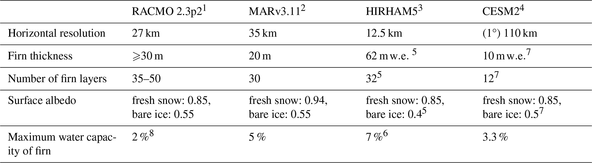
¹ Van Wessem et al. (2018); ² Kittel et al. (2021); ³ Boberg et al. (2022); ⁴ Danabasoglu et al. (2020); ⁵ Hansen et al. (2021); ⁶ Langen et al. (2017); ⁷ van Kampenhout et al. (2017); ⁸ Ettema et al. (2010)

2.1.1 CESM2.1

The Community Earth System Model version 2.1 (CESM2) is a global climate model from the Coupled Model Intercomparison Project phase 6 (CMIP6) generation (Danabasoglu et al., 2020), developed by the National Center for Atmospheric Research (NCAR). It interactively integrates the atmosphere (Gettelman, 2019), ocean and sea ice (Hunke and Lipscomb, 2010), and land surface components (Lawrence et al., 2019), with a nominal horizontal resolution of 1-degree (≈110 km) finite volume grid (f09_g16). Its land surface component incorporates an advanced representation of snowpack processes (van Kampenhout et al., 2017), with a 12-layer stratification spanning a firn column with 10 m water equivalents (w.e.) (Lawrence et al., 2019; van Kampenhout et al., 2020). Snow albedo is computed across five spectral bands in the visible and in the near-infrared and primarily depends on grain size, density, and the presence of impurities (Flanner and Zender, 2005; Flanner et al., 2007). Finally, firn is initialized through a long spin-up, allowing the model to reach a quasi-steady state of densification, percolation/refreezing, and grain-size evolution consistent with the imposed climate forcing (van Kampenhout et al., 2017).

In this study, we use a CESM2 member specifically produced at Utrecht University (van Kampenhout et al., 2020), which was branched in 1950 from the CMIP6 historical simulation and follows the CMIP6 experimental protocol. This member is not part of the official CMIP6 ensemble but was generated to provide the 6-hourly three-dimensional atmospheric fields required to drive RCMs at their lateral and surface boundaries, at a time when the official CESM2 runs for CMIP6 at NCAR did not archive variables at this temporal resolution.

CESM2 was selected as the common forcing for the three RCMs for several reasons. First, it was among the first CMIP6 ESMs to provide high-frequency (6-hourly) atmospheric forcing data both at the surface and throughout the entire atmospheric column (3D), required for driving RCMs at their boundaries. In addition, CESM2 has emerged as one of the best-performing models in an intercomparison exercise assessing the ability of CMIP6 ESMs to simultaneously represent contemporary climate at both poles (Agosta et al., 2022). Finally, the level of detail in its land-surface scheme, through coupling with the Community Land Model version 5 (CLM5), allows for an advanced representation of the SMB components, including snow accumulation, melt, refreezing, and runoff (van Kampenhout et al., 2017; Lawrence et al., 2019; Dunmire et al., 2022). This detailed representation of the various SMB components makes CESM2 outputs directly comparable with those of the RCMs, enabling a consistent intercomparison.

2.1.2 RACMO 2.3p2

The Regional Atmospheric Climate Model (RACMO) is developed by the Royal Netherlands Meteorological Institute (KNMI), with its polar component primarily maintained at the Institute for Marine and Atmospheric Research Utrecht (IMAU). The simulations analyzed in this study are based on the Antarctic runs of RACMO2.3p2 at 27 km horizontal resolution (Van Wessem et al., 2018). For simplicity, this version is hereafter referred to as RACMO. It has been widely used to simulate the climate of the Greenland (Noël et al., 2018) and Antarctic (Van Wessem et al., 2018) ice sheets. RACMO combines the hydrostatic dynamical core of the HIRLAM model with the CY33r1 physics package of the European Centre for Medium-Range Weather Forecasts (ECMWF). Its snow scheme represents a maximum of 100 layers, but in practice it varies around 35–50 layers (typically 35 for ablation areas and up to 50 for high accumulation areas after long runs), discretized over a depth of at least 30 m. In RACMO, snow albedo is calculated through a prognostic scheme for snow grain size, modulated by cloud cover and solar zenith angle (Munneke et al., 2011). The firn column is initialized using climatological profiles of temperature, density, and liquid water content derived from the IMAU Firn Densification Model (IMAU-FDM) (Ligtenberg et al., 2011). The model employs topographic data from Cook et al. (2012) and Bamber et al. (2009).

2.1.3 MARv3.11

The Regional Atmospheric Model (MAR) is mainly developed at the University of Liège in Belgium. The version of the model employed in this study is MARv3.11, specifically developed for Antarctica and run at a horizontal resolution of 35 km (Agosta et al., 2019). For simplicity, this version is hereafter referred to as MAR. It has been widely used to simulate the climate in high latitudes, including Antarctica (e.g. Kittel et al., 2021) and Greenland (e.g. Fettweis et al., 2017). The atmospheric dynamics of MAR are based on the hydrostatic approximation of the primitive equations (Gallée and Schayes, 1994), while its microphysics scheme employs prognostic equations for five water species: specific humidity, cloud droplets, ice crystals, raindrops, and snow particles (Gallée, 1995). Its snow scheme represents 30 layers (with time varying thickness) discretized over a depth of 20 m. MAR dynamically computes surface albedo based on snow properties (grain size, density), zenithal angle as well as cloud cover (Tedesco et al., 2016). The snowpack is initialized with zero liquid water content, temperature and density profiles from a prior simulation over the contemporary period, followed by a spin-up phase, corresponding to the initialization time required for the model to reach a thermodynamic equilibrium between the surface and atmosphere consistent with its boundary conditions. The topography used in MAR is derived from the Bedmap2 surface elevation dataset (Fretwell et al., 2013).

2.1.4 HIRHAM5

The regional climate model HIRHAM (Christensen et al., 2007) results from the combination of the numerical weather prediction model HIRLAM7 (Eerola, 2006) and the hydrostatic general circulation model ECHAM5 (Roeckner et al., 2003). This model has been developed through a collaboration between the Danish Climate Centre of the DMI (Danish Meteorological Institute) and the Alfred Wegener Institute (AWI), Helmholtz Centre for Polar and Marine Research. The simulations analyzed in this study are based on HIRHAM5, hereafter referred to simply as HIRHAM, which has been optimized to represent the Greenland climate and run in Antarctica at a horizontal resolution of 12.5 km (Boberg et al., 2022). While HIRHAM does include a coupled surface energy and mass budget scheme over ice sheets, its subsurface snow/ice representation has only few (5) widely spaced layers, and the results presented here are therefore from an offline SMB model instead. This means that the surface scheme is forced by atmospheric outputs but does not feed back on the atmosphere during the simulation. The snowpack thickness is 60 m water equivalent (w.e.), subdivided into 32 layers, and firn density evolves under overburden pressure using established compaction schemes (Langen et al., 2017). In HIRHAM5, surface albedo is a linear function of surface temperature, with a minimum value of 0.65 at the melting point and a maximum value of 0.85 for surface temperatures of −5 °C and below (Lucas-Picher et al., 2012). Albedo is also influenced by cloud cover and the solar zenith angle. The snowpack is initialized through a 50-year spin-up, based on a prescribed profile derived from historical simulations. At the start of the spin-up, the deep temperature in the bottom layer is initialised as the mean annual temperature from the RCM's first 10 years. This decadal time series is repeated offline until the snowpack reaches equilibrium. It is then used as a starting condition in the HIRHAM model as it is run into the future. Liquid water (melt and rain) percolate into the snow and refreeze according to the cold content of the layers, the mass of which is tracked using an Eulerian scheme. Full details are given in Hansen et al. (2024); Langen et al. (2017). The topography used in HIRHAM is derived from the GTOPO30 surface elevation dataset (Mottram et al., 2021).

2.2 Comparative of parameterizations

When comparing projections from the different models, it is crucial to consider the specific parameterizations implemented in each RCM (Table 1). One key difference lies in how atmosphere–surface interactions are handled: HIRHAM operates with a decoupled atmosphere–surface setup, whereas MAR, RACMO, and CESM2 employ fully interactive coupling, allowing feedbacks from the surface to influence the atmosphere. The models also differ in the initialization of their snow and firn schemes, and all use a different spin-up method. Total snowpack thickness ranges from 20 m in MAR to 62 $\mathrm{m}\mathrm{w}.\mathrm{e}.$ in HIRHAM, when it is variable in RACMO and set to 10 $\mathrm{m}\mathrm{w}.\mathrm{e}.$ in CESM2, while the vertical layering varies in both number and thickness of layers in the four models. Percolation – the downward movement of liquid water within the snowpack – is represented in MAR, RACMO, and CESM2 using a bucket-type approach: once a layer reaches its maximum water retention capacity (also known as irreducible water saturation), excess water is passed to the layer below, and any remaining water that is not retained in the firn or refrozen within the current time step contributes to runoff. In all four models, runoff is treated as a purely vertical process and does not account for lateral water fluxes. HIRHAM follows a more physical approach in which the vertical flow of liquid water is governed by a Darcy's law (Langen et al., 2017). In any of these strategies, the efficiency of the percolation process depends on the water retention capacity, defined as a percentage of the available pore space of each layer, which differs between models from a fixed 2 % in RACMO (Ettema et al., 2010) to a maximum set to 7 % per layer in HIRHAM (Machguth et al., 2026). Albedo specifications for fresh snow and bare ice also vary across models, directly affecting the strength of the melt–albedo feedback. Lower albedo values, for instance, enhance melt through increased absorption of solar radiation. These parametric and structural differences are important sources of variability in ice sheet surface mass balance projections, as highlighted in previous comparative studies over Antarctica (Mottram et al., 2021) and Greenland (Fettweis et al., 2020; Glaude et al., 2024).

2.3 Intercomparison protocol

For the purpose of inter-model comparison, all outputs from the four models were bi-linearly interpolated onto a common 10 km regular stereographic polar grid (EPSG3031), which differs from and is finer than the native grids of each model. This is especially significant for CESM2, whose native grid (100 km) is an order of magnitude coarser than the common grid, so that the interpolation adds no real small-scale information. This grid has been adopted from the Ice-sheet Model Intercomparison Project phase 6 (ISMIP6) (Seroussi et al., 2020). A common ice mask, defined as the maximum ice extent common to the four models, was also applied to each model to ensure comparisons over identical areas, as previous studies demonstrate that considering different ice masks can have a major impact on SMB results (Hansen et al., 2022). The digital elevation model used to generate model topography on each model's native grid differs among the four models (Sect. 2.1). This leads to differences in surface elevation between models. While RCMs generally show good agreement with differences most pronounced in areas of steep topographic gradients, CESM2 generally features higher elevations over ice shelves and lower elevations over grounded ice (Fig. S1 in the Supplement). The 1995–2014 period was chosen as the 20-year contemporary reference, during which Antarctic SMB remained relatively stable (Mottram et al., 2021), in line with ISMIP6 recommendations (Seroussi et al., 2020).

In order to compare the four models on an equal footing, the analysis is primarily conducted in terms of anomalies with respect to their own present day climate. We refer to “future anomalies” as the difference between the mean of the 2080–2099 period and that of the reference period 1995–2014, and into “time series anomalies” as the deviation of each annual value from this same reference mean. This approach highlights projected trajectories while minimizing the influence of systematic biases that may arise from parametric and structural differences between the models and the resulting representation of the contemporary climate. Furthermore, by defining the reference period as representative of a stable climate (Mottram et al., 2021), each model can establish its own equilibrium state, particularly with respect to the surface energy balance. However, differences in this initial equilibrium affect both the magnitude and direction of projected long-term anomalies. Therefore, to identify the mechanisms underlying inter-model discrepancies, this anomaly-based analysis is complemented by an evaluation in absolute values.

Both the anomalies and absolute values discussed above are derived from annual mean or cumulative quantities rather than seasonal (e.g. austral summer, DJF) values, even though the processes discussed here (melt, runoff, melt-albedo feedback) are primarily active during the summer months. This choice is dictated by the structure of the available model output: the projections were produced and archived on an annual calendar basis through 2100, and monthly or seasonal components are not available for this analysis. As a result, all quantities presented throughout this study are restricted to annual means and cumulative values, a limitation that should be kept in mind when interpreting the inter-model comparisons.

In addition to the future projections discussed above, present-day model performance is also evaluated using historical simulations forced by ERA5 reanalysis over the 1980–2022 period, for which daily output is available. This higher temporal resolution allows for a direct comparison against daily satellite-derived melt products, namely AMSR2 and SSM/I (Picard et al., 2022), which are used in Sect. 3.1.2 to evaluate melt extent and duration across models. Following Torinesi et al. (2003), model and satellite-derived melt fields are compared using three metrics: the Cumulative Melting Surface (CMS; d km²), defined as the spatial yearly (calendar year) sum of melt days multiplied by the pixel area (10 km×10 km); the Maximum Melting Surface (MMS; km²), corresponding to the surface over which melting is detected at least once during the corresponding year; and the Mean Melt Duration (MMD; d), obtained by dividing the CMS by the MMS.

3 Results

In this section we first compare RCM simulations driven by CESM2 and ERA5, assess inter-model differences regardless of the chosen forcing over the contemporary period, and evaluate modeled melt days against satellite observations (Sect. 3.1). Second, we examine SMB projections and their individual components to identify the main contributors to inter-model variability (Sect. 3.2). Finally, we provide a detailed analysis of these components to determine the drivers of SMB variability projected by the end of the century (Sect. 3.3).

3.1 Evaluation

3.1.1 Evaluation of dynamical downscalings over the contemporary period

Before analyzing projections, it is essential to assess the ability of the three RCMs driven by CESM2 to reproduce a realistic SMB over the contemporary period. To this end, we compare their dynamical downscalings of CESM2 to their respective reference versions driven by ERA5 over the 1995–2014 reference period, all interpolated to a common grid of 10 km resolution. Table 2 shows that integrated SMB estimates over the common ice mask are very close between the two forcings for each RCM, with differences of 38, 51, and 30 Gt yr⁻¹ for HIRHAM, MAR, and RACMO, respectively. These differences are well below the interannual variability (standard deviation over the period) by factors between 1.7–3, confirming that CESM2 downscalings are in good agreement with the ERA5-driven reference simulations. Figure 1 illustrates the spatial SMB differences between CESM2- and ERA5-driven simulations, with hatching indicating areas where differences are smaller than or equal to the interannual SMB variability in the ERA5-driven simulations. A consistent spatial pattern of deviations is observed across the three RCMs, suggesting that the differences mainly originate from the CESM2 forcing itself, linked to distinct atmospheric circulation regimes between CESM2 and ERA5, rather than the RCM used. For example, as shown in Fig. 1, CESM2-driven RCMs overestimate SMB in the region spanning from the Antarctic Peninsula through Queen Maud Land to the Amery Ice Shelf, a direct consequence of CESM2's overestimation of precipitable water and sea-level pressure in this area (Kittel et al., 2021). Underestimation is also observed in Wilkes Land and the periphery of West Antarctica. While strong performance under present-day conditions does not necessarily guarantee accurate projections, it is a necessary prerequisite. These results therefore support the use of CESM2 downscalings as sufficiently reliable for the analysis of climate projections presented in the remainder of this study.

Table 2 Integrated values over the contemporary period (1995–2014) of SMB, precipitation (PR), runoff (RU), melt (ME), and refreezing (RF), integrated over the entire Antarctic ice sheet in Gt yr⁻¹ for the three models driven by CESM2 and ERA5.

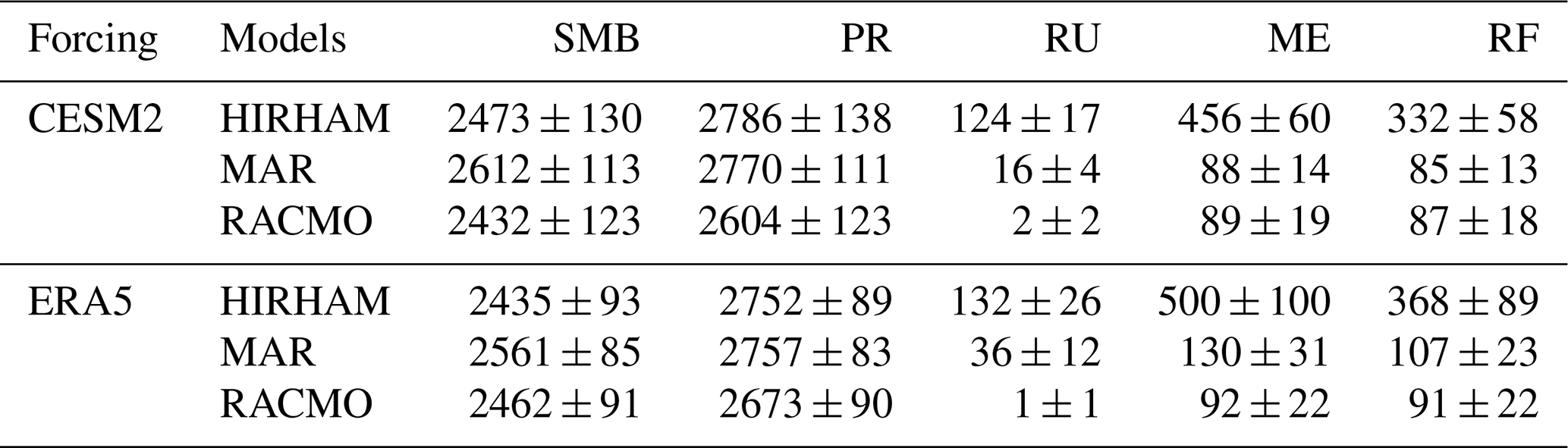
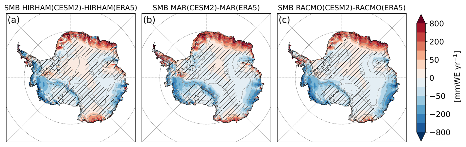
Figure 1 Differences in mean Antarctic SMB simulated by the RCMs: HIRHAM (a), MAR (b), and RACMO (c), driven by CESM2 and ERA5, in $\mathrm{mm}\mathrm{w}.\mathrm{e}.{\mathrm{yr}}^{-\mathrm{1}}$, over the reference period 1995–2014. Hatched areas indicate regions where the differences are smaller than the interannual variability (standard deviation over the period) of the SMB from RCMs driven by ERA5.

Although the integrated SMB values are quite close across the models (with differences between 2 %–7 %), their individual components (Table 2) reveal pronounced inter-model differences that appear largely independent of the forcing used. In particular, HIRHAM consistently produces substantially higher melt rates and runoff than MAR and RACMO over the present-day period, in line with previous assessment of HIRHAM when driven by reanalysis (Boberg et al., 2022). For instance, HIRHAM simulates melt rates approximately five times greater than those of the other two RCMs, accompanied by refreezing about four times higher than in MAR and RACMO. This refreezing partially suppresses melt, yet significant runoff still occurs, amounting to 124±17 Gt yr⁻¹ for CESM2-driven HIRHAM and 132±26 Gt yr⁻¹ for ERA5-driven HIRHAM, compared with only 16±4 and 36±12 Gt yr⁻¹ for MAR, and 2±2 and 1±1 Gt yr⁻¹ for RACMO. The similarity of these magnitudes between the two forcings for a given RCM clearly indicates that these differences arise from the intrinsic regional model physics rather than the atmospheric forcing. This is particularly important given that the temperature–melt relationship is non-linear due to the positive melt–albedo feedback (Jakobs et al., 2021a). These results suggest that in HIRHAM the firn layer loses its meltwater retention capacity more rapidly, promoting runoff in response to an increase in surface liquid water.

3.1.2 Evaluation of RCMs melt days

Each RCM has already been individually and extensively evaluated against SMB and near-surface meteorological observations (e.g. Kittel et al., 2021; Van Wessem et al., 2018; Mottram et al., 2021). However, to assess the ability of the three RCMs to represent surface melt within our intercomparison protocol, we compare the simulated number of surface melt days – defined using a threshold of 1 mm d⁻¹ as in Donat-Magnin et al. (2020), owing to the strong sensitivity of microwave signals to surface meltwater (Picard et al., 2022) – with satellite observations from the Advanced Microwave Scanning Radiometer 2 (AMSR2) and the Special Sensor Microwave/Imager (SSM/I). These satellite sensors allow the detection of liquid water at or close to the snowpack surface. The satellite data were regridded to the ISMIP6 10 km grid and the daily RCM outputs used for this comparison originate from a dynamical downscaling of ERA5.

Figure 2 shows the Cumulative Melting Surface (CMS; d km²) (Fig. 2a), the Maximum Melting Surface (MMS; km²) (Fig. 2b) and the Mean Melt Duration (MMD; d) (Fig. 2c), all defined in Torinesi et al. (2003). CMS represents the spatial yearly (calendar year) sum of melt days multiplied by the pixel area (10 km×10 km). The MMS corresponds to the surface over which melting is detected at least once during the corresponding year, and the MMD is calculated by dividing the CMS by the MMS. At the 1 mm d⁻¹, both MAR and RACMO show good agreement with the observations, with a Normalized Root Mean Square Error (NRMSE, Eq. S1 in the Supplement) on MMD of 15 % and 21 % when compared with SSM/I, and 17 % and 32 % with AMSR2. In contrast, HIRHAM presents significantly more mean melt days, with an NRMSE of 135 % and 104 % for SSM/I and AMSR2, respectively. Note that for HIRHAM the statistics show little sensitivity to the choice of the daily threshold compared to MAR and RACMO, owing to its much higher melt rates. For HIRHAM, increasing the threshold up to 3 mm d⁻¹ has only a limited impact on MMD, since most melt days already exceed this value; the NRMSE relative to SSM/I only decreases from 135 % to 109 %, and a threshold close to 10 mm d⁻¹ is required for HIRHAM to approach the observed MMD. By contrast, for MAR and RACMO, a 3 mm d⁻¹ threshold excludes a larger fraction of melt days, which has a stronger effect on MMD: the NRMSE relative to SSM/I increases from 15 % to 24 % and from 21 % to 35 %, respectively.

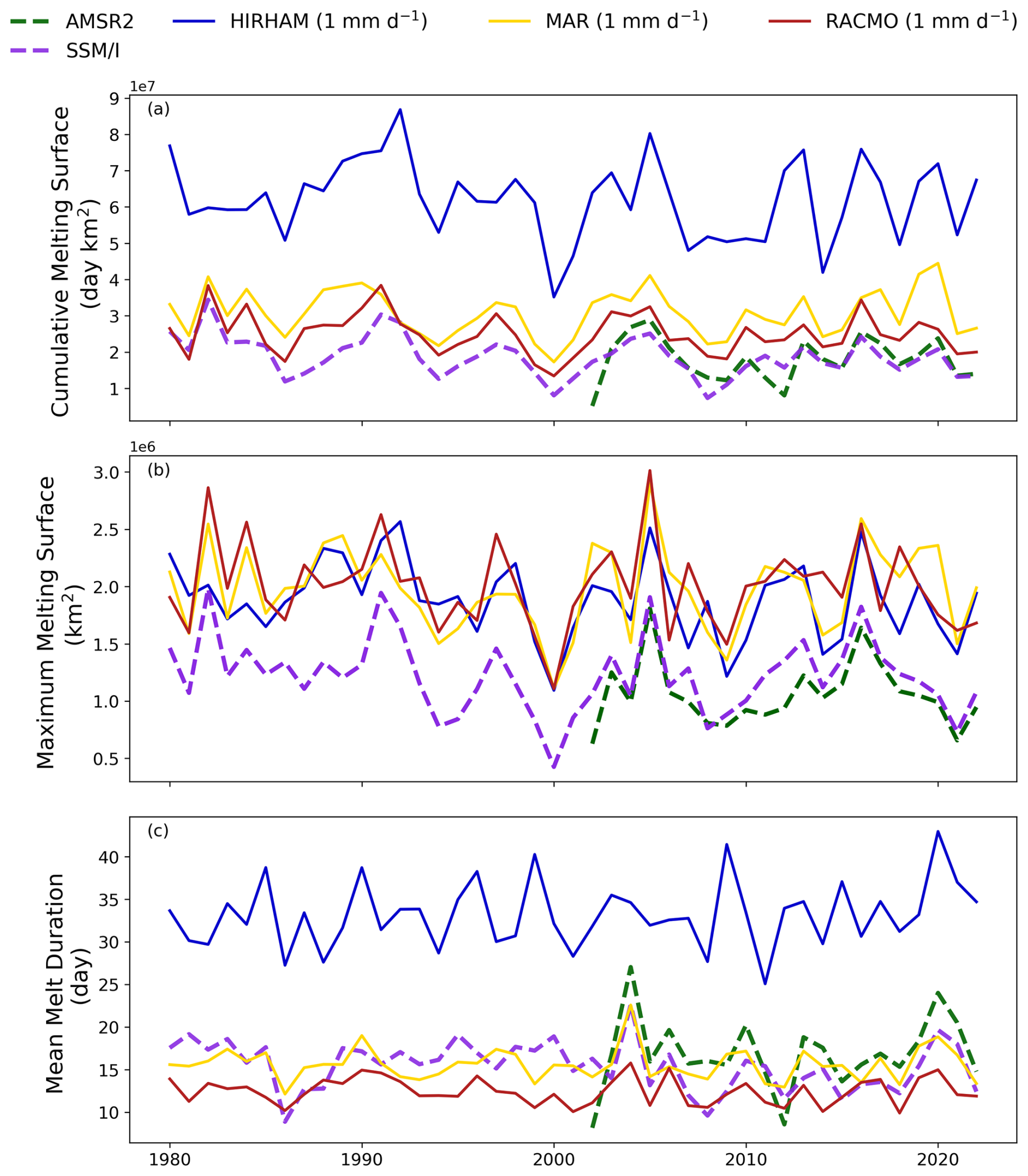
Figure 2 Annual time series (calendar years) of the Cumulative Melting Surface (CMS; d km²) (a), the Maximum Melting Surface (MMS; km²) (b), and the Mean Melt Duration (MMD; d) (c) during the period 1980–2022. For the models MAR (yellow), HIRHAM (blue), and RACMO (red), driven by ERA5 at thresholds of 1 mm d⁻¹. For the satellite observations AMSR2 (green, dashed line) and SSM/I (purple, dashed line).

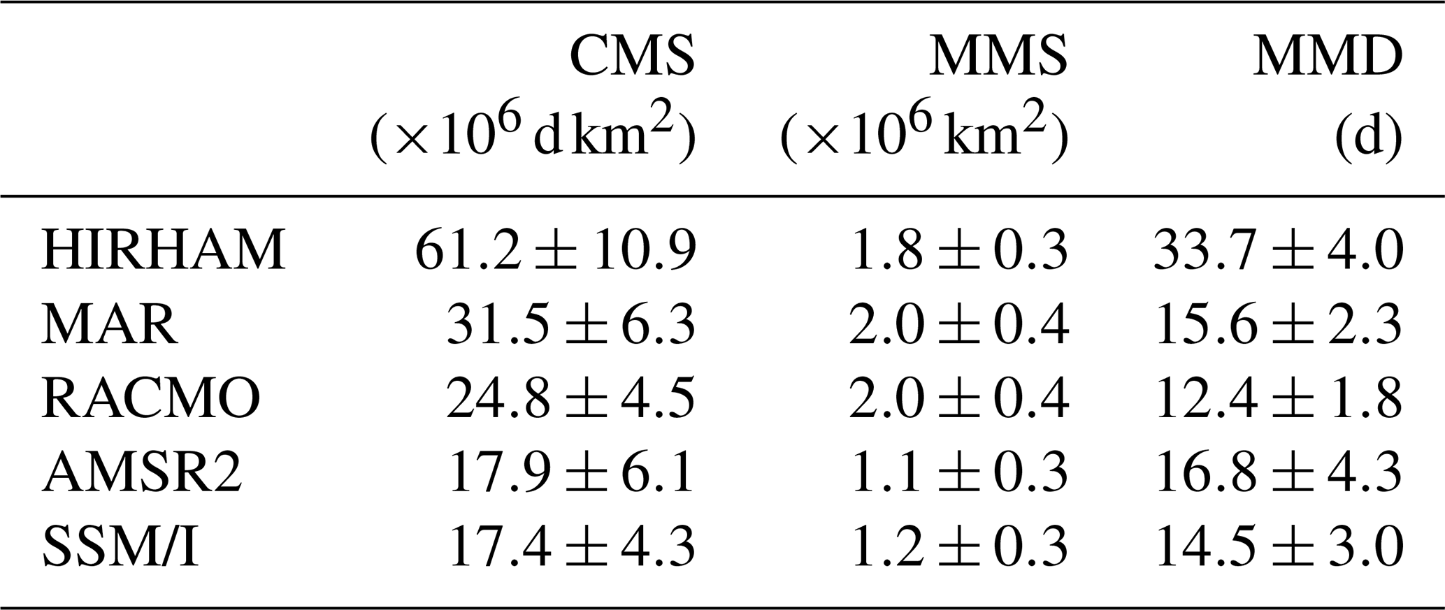
On Fig. 2b, MMS shows that HIRHAM produces melt over surfaces of similar extent to those of MAR and RACMO (ranging between 2.0×10⁶–1.8×10⁶ km² for the models), which are all above the observed melting surface (1.1×10⁶ and 1.2×10⁶ km² for ASMR2 and SSM/I; Table 3). We also note the fact that for HIRHAM, the difference in the threshold does not significantly impact the total extent of the melting surface. Figure 2 highlights several points: first, MAR and RACMO faithfully represent the observations, confirming previous findings regarding surface melting (e.g. Kuipers Munneke et al., 2012; Kittel et al., 2021; Van Wessem et al., 2023). Second, HIRHAM produces significantly more melt over approximately the same melting areas, which is attributed to its high melt rates. This discrepancy is reflected in the MMD (Fig. 2c), where HIRHAM simulates an average melt duration of 33.7±4.0 d across the melting area, compared to 16.8±4.3 and 14.5±3.0 d for AMSR2 and SSM/I, respectively (Table 3). This confirms that the major deviation in CMS results from the model sustaining melt for a longer average period even with high melt rates threshold.

Table 3 Means values of Cumulative Melting Surface (CMS; d km²), Maximum Melting Surface (MMS; km²) and Mean Melting Duration (MMD; d) over the period (1980–2022) for HIRHAM, MAR, RACMO, and SSM/I and over (2002–2022) for AMSR2. The threshold of 1 mm d⁻¹ is used for models. The standard deviation represents the interannual variability.

3.2 Inter-model comparison of SMB projections

Figure 3 shows SMB future anomalies over the entire Antarctic Ice Sheet for the period 2080–2099 relative to 1995–2014, expressed in $\mathrm{mm}\mathrm{w}.\mathrm{e}.{\mathrm{yr}}^{-\mathrm{1}}$ (Fig. 3a–d). All four models, HIRHAM (Fig. 3a), MAR (Fig. 3b), RACMO (Fig. 3c), and CESM2 (Fig. 3d), show a clear contrast between the grounded ice sheet, characterized by increased SMB (positive anomalies), and the floating ice shelves, which mostly experience a decline in SMB (negative anomalies). The locations mentioned hereafter are illustrated Fig. S2. In HIRHAM, all ice shelves exhibit negative anomalies. MAR simulates a more localized decrease, notably over the Amery ice shelf, along the ice shelves of Queen Maud Land and over Larsen ice shelf. RACMO shows relatively stable SMB across most ice shelves, close to present-day equilibrium, except over Larsen ice shelf and a few shelves in Queen Maud Land, where negative anomalies also appear. In CESM2, negative anomalies are primarily observed over the Antarctic Peninsula and along the ice shelves of Queen Maud Land. In MAR, RACMO, and CESM2, the large Ronne–Filchner and Ross ice shelves maintain generally positive anomalies. In addition, MAR shows negative SMB values along parts of the grounding lines of the Ross and Ronne–Filchner ice shelves. These localized deficits are very likely related to interactions between the local atmospheric circulation and the Transantarctic Mountains, including foehn-induced or adiabatic warming, as well as enhanced snowfall sublimation (Agosta et al., 2019). Over the grounded ice sheet, all four models consistently indicate a general increase in SMB, with similar spatial patterns: stability over the Antarctic plateau and a pronounced SMB increase in the western part of the ice sheet.

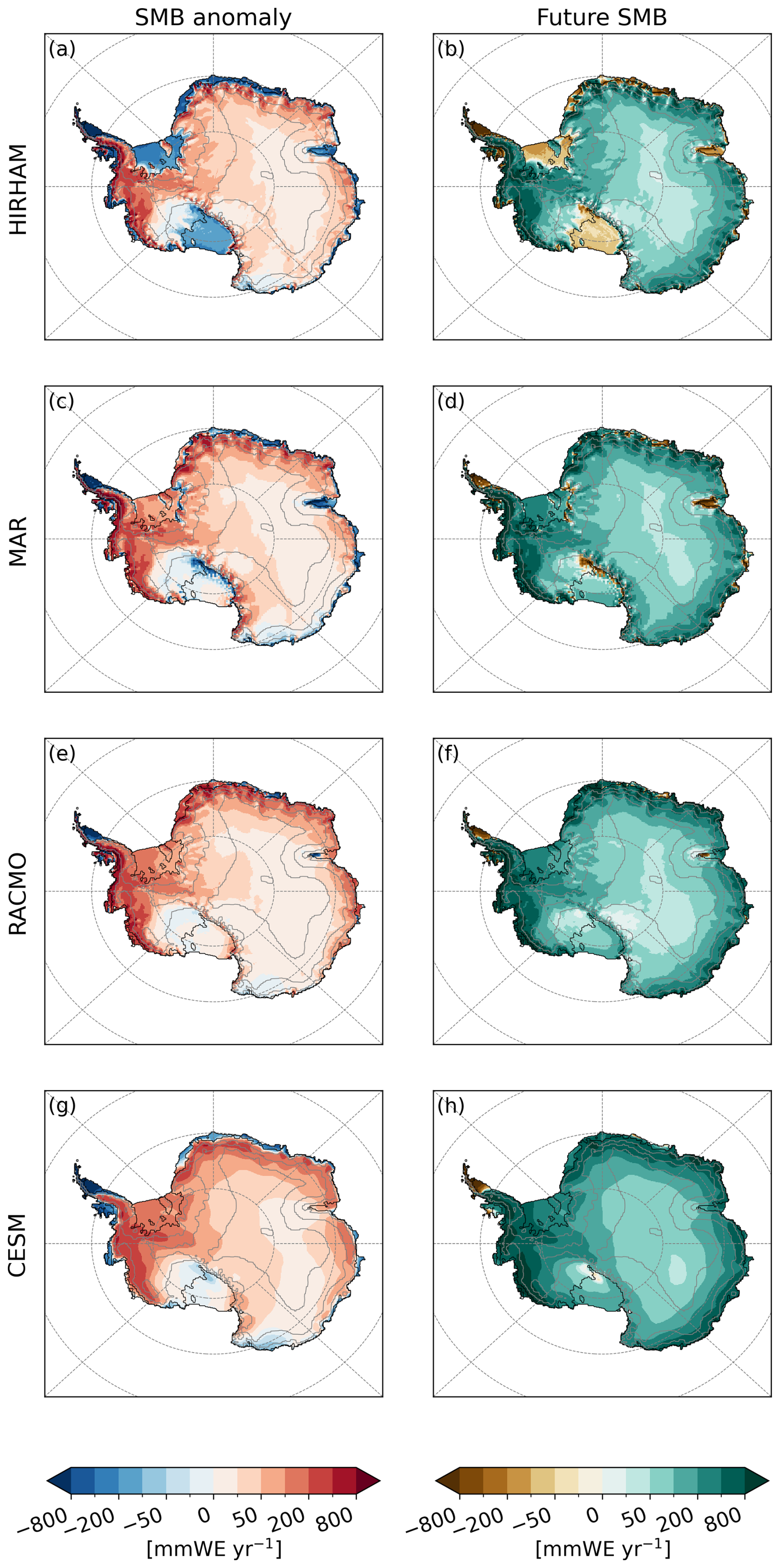
Figure 3 SMB anomaly between the means of 2080–2099 and 1995–2014; HIRHAM (a), MAR (b), RACMO (c), and CESM2 (d) and mean future SMB over 2080–2099; HIRHAM (e), MAR (f), RACMO (g), and CESM2 (h), in $\mathrm{mm}\mathrm{w}.\mathrm{e}.{\mathrm{yr}}^{-\mathrm{1}}$, under the SSP5-8.5 scenario.

Future SMB means for the period 2080–2099 (Fig. 3d–f) confirm these trends, with enhanced ablation in HIRHAM, where most ice shelves exhibit negative SMB. In MAR and RACMO, negative values are primarily confined to the Antarctic Peninsula and the Amery Ice Shelf. In CESM2, only the tip of the Antarctic Peninsula shows negative SMB. Moreover, relative to the RCMs, CESM2 reproduces a relatively latitudinally homogeneous field with high values, dominated by a coast-to-plateau gradient. This pattern directly reflects the limited horizontal resolution, which controls the representation of topographic gradients and influences orographic precipitation in the model, particularly visible along the margins of Queen Maud Land, in West Antarctica, and around the Amery Ice Shelf. Given this pronounced distinction between grounded and floating regions, and to avoid obscuring their divergent SMB trajectories, we choose to analyze them separately for the remainder of the study.

Under warmer conditions, the continent-scale SMB is primarily governed by precipitation (the main accumulation component at the surface) and runoff (the main ablation component); sublimation, although locally significant, remains relatively minor at the continental scale (Kittel et al., 2021). Figure 4 shows the temporal evolution of SMB, precipitation, and runoff anomalies integrated over the grounded ice and the ice shelves. These time series highlight inter-model consistency over the grounded ice, but pronounced differences on the ice shelves by 2100.

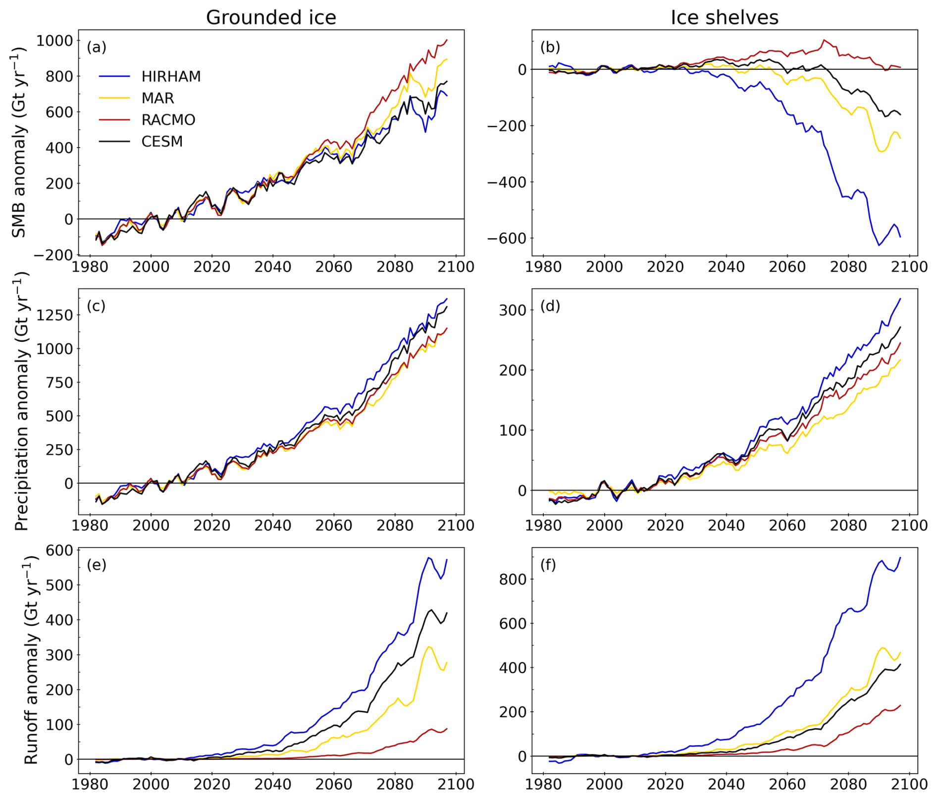
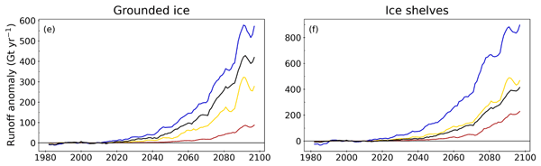
Figure 4 Time series anomalies of SMB (a, b), precipitation (c, d), and runoff (e, f), in Gt yr⁻¹, relative to the reference period 1995–2014. For the models MAR (yellow), HIRHAM (blue), and RACMO (red), driven by CESM2 (black) under the SSP5-8.5 scenario. Values are integrated over the grounded (left) and floating (right) parts of the Antarctic ice sheet. Note that the y axis scales differ between grounded and floating ice due to the difference in surface areas. A 5-year running mean is applied for clarity.

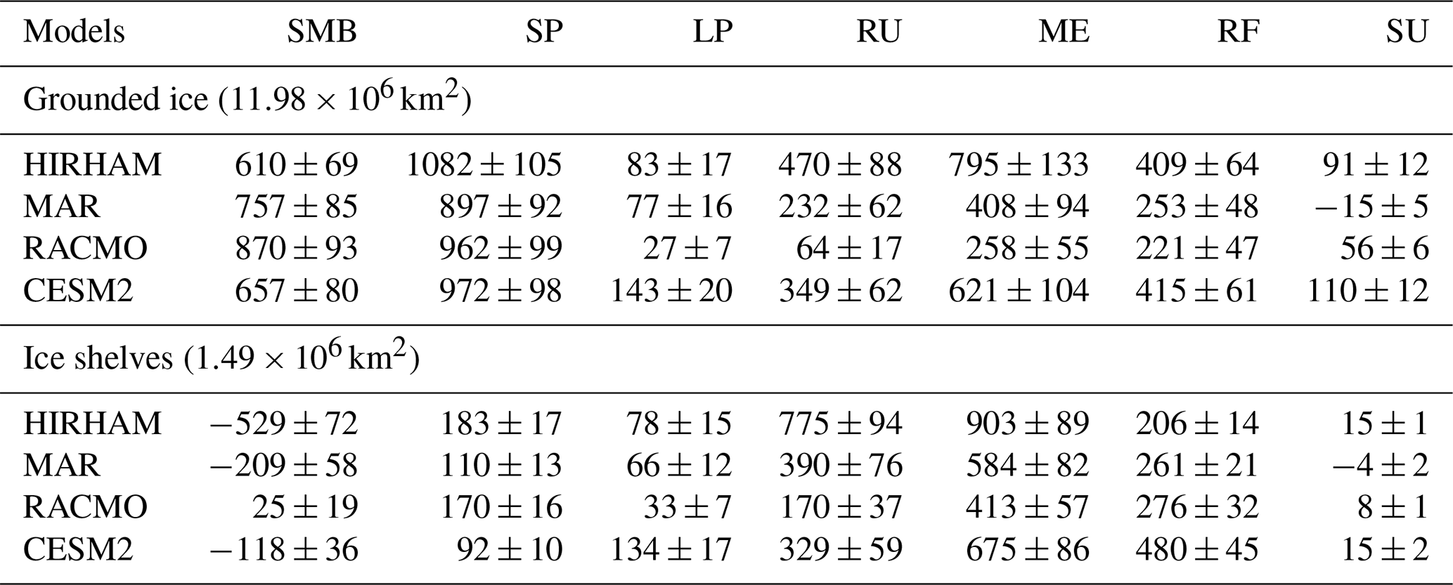
Over the grounded ice sheet, the models consistently project an increase in SMB by the end of the century (Fig. 4a), with future anomalies for 2080–2099 ranging from $+\mathrm{610}\pm \mathrm{69}$ Gt yr⁻¹ for HIRHAM to $+\mathrm{870}\pm \mathrm{93}$ Gt yr⁻¹ for RACMO (Table 4). Despite differences in runoff (Fig. 4e), grounded SMB is largely dominated by precipitation, with anomalies ranging from $+\mathrm{974}\pm \mathrm{111}$ Gt yr⁻¹ for MAR to $+\mathrm{1171}\pm \mathrm{122}$ Gt yr⁻¹ for HIRHAM (Table 4). In contrast, projections for the ice shelves reveal substantial divergence (Fig. 4b). RACMO simulates a nearly stable SMB, close to present-day equilibrium, with an anomaly of $+\mathrm{25}\pm \mathrm{19}$ Gt yr⁻¹, resulting from a near balance between runoff ($+\mathrm{170}\pm \mathrm{37}$ Gt yr⁻¹) and precipitation ($+\mathrm{203}\pm \mathrm{23}$ Gt yr⁻¹, Table 4). Conversely, HIRHAM, MAR and CESM2 indicate net surface mass loss, with anomalies of $-\mathrm{529}\pm \mathrm{72}$, $-\mathrm{209}\pm \mathrm{58}$, and $-\mathrm{118}\pm \mathrm{36}$ Gt yr⁻¹, respectively. These losses result from increased runoff that is no longer compensated by precipitation: runoff anomalies reach $+\mathrm{775}\pm \mathrm{160}$ Gt yr⁻¹ for HIRHAM, $+\mathrm{390}\pm \mathrm{76}$ Gt yr⁻¹ for MAR, and $+\mathrm{329}\pm \mathrm{59}$ Gt yr⁻¹ for CESM2. Such intermodel spread is striking at the end of the century, with HIRHAM exhibiting the highest runoff rates of about 4.6 times those of RACMO, which is the model that has the most constant SMB.

Table 4 Future integrated anomalies of SMB, solid (SP) and liquid precipitation (LP), runoff (RU), melt (ME), refreezing (RF), and sublimation (SU), calculated as the mean for 2080–2099 relative to the reference period 1995–2014, in Gt yr⁻¹. For HIRHAM, MAR, and RACMO driven by CESM2 and CESM2 under the SSP5-8.5 scenario, over the grounded ice and ice shelves. The standard deviations (±) indicate high confidence that the integrated anomalies are all statistically different from zero. All anomalies exceed interannual variability (i.e. the standard deviation) and are therefore considered significant.

These contrasts reflect not only differences in runoff magnitude but also in the timing of negative anomalies emergence over ice shelves: HIRHAM anticipates a transition to negative SMB anomalies as early as 2040, whereas it appears only around 2060 for MAR and 2070 for CESM2. Thus, inter-model dispersion over the ice shelves largely stems from the representation of runoff, in both its intensity and temporal evolution. To reduce dependence on emission scenario timing, the following analysis considers SMB component evolution as a function of the climate response (near-surface air temperature) rather than absolute time.

3.3 Processes driving inter-model differences in SMB projections

Under warmer conditions, several mechanisms can enhance both the frequency and magnitude of surface runoff over the ice sheet: increased rainfall, greater liquid-water production driven by cloud-emitted longwave radiation (e.g. Kittel et al., 2022) and by the melt–albedo feedback, and a diminished water-retention capacity of the firn. Figure 5 presents annual (calendar year) near-surface air temperatures for the four models, highlighting persistent differences of 2–3 °C over both grounded ice and ice shelves. Given the strong temperature dependence of surface melt and the inter-model differences in near-surface temperature, the following results are discussed in terms of absolute near-surface temperature (note that these discrepancies are only negligibly affected by differences in topography; see Fig. S3). This approach allows us to account for the structural differences between models and to highlight their present-day states, rather than focusing solely on their temporal evolution. Moreover, to make the discussion clearer, and since the differences are driven by distinct physical mechanisms, we focus first on HIRHAM's evolution, before considering how MAR, RACMO, and CESM2 diverge from one another.

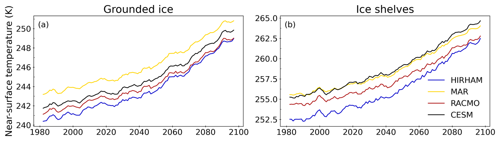
Figure 5 Time series of near-surface temperature, in K. For the models MAR (yellow), HIRHAM (blue), and RACMO (red) driven by CESM2 (black) under the SSP5-8.5 scenario. Values are integrated over grounded (left) and floating (right) parts of the ice sheet. Note that the y axis scales differ between grounded and floating ice due to the difference in surface areas. A 5-year running mean is applied for clarity.

The melt–albedo feedback is known to be a key driver of melt rate evolution and a strongly nonlinear process (e.g. Jakobs et al., 2021a). Albedo directly controls the net shortwave radiation (SWN); hence, SWN anomalies are used here to represent albedo changes. Focusing first on the ice shelves, HIRHAM projects the strongest increase in SWN by the end of the simulation $+\mathrm{6.76}\pm \mathrm{0.41}$ W m⁻², compared to $+\mathrm{0.32}\pm \mathrm{0.11}$ W m⁻² for MAR, $+\mathrm{0.68}\pm \mathrm{0.22}$ W m⁻² for RACMO, and $+\mathrm{1.27}\pm \mathrm{0.18}$ W m⁻² for CESM2 (Fig. 6b). This pronounced anomaly in HIRHAM clearly indicates that the melt–albedo feedback strongly amplifies simulated melt rates.

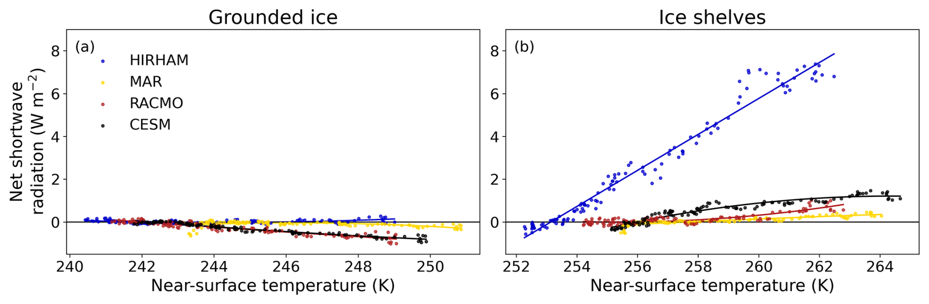
Figure 6 Net shortwave radiation (SWN), in W m⁻² as function of the absolute annual near-surface air temperature in K. For the models MAR (yellow), HIRHAM (blue), and RACMO (red) driven by CESM2 (black) under the SSP5-8.5 scenario. Mean values over grounded (left) and floating (right) parts of the ice sheet. A 5-year running mean is applied for clarity.

The runaway of this positive feedback can be linked to HIRHAM's already elevated contemporary melt and refreezing. HIRHAM melt and refreezing exceeds by factors of 5 and 4 from those of MAR and RACMO, and by factors of 3 and 2 from those of CESM2 over the ice shelves, based on mean values for the period 1995–2014 (Table S1 in the Supplement). Moreover, because HIRHAM starts from slightly lower temperatures (252 K), when we compare its melt and refreezing rates with those at the starting temperatures of RACMO (254 K), MAR and CESM2 (255 K), its rates already match those projected at the end of the simulation under a high-emission scenario (Fig. 7b and d). The combination of early high melt rates and distinct SWN evolution results in considerably higher projected melt for HIRHAM, mainly driven by the melt–albedo feedback. As shown in Fig. 7, HIRHAM's melt, refreezing and runoff (panels a-d and g-h) stand out throughout the simulation. The projected melt anomalies over the ice shelves reach $+\mathrm{903}\pm \mathrm{90}$ Gt yr⁻¹ for HIRHAM, compared to $+\mathrm{584}\pm \mathrm{84}$ Gt yr⁻¹ for MAR, $+\mathrm{413}\pm \mathrm{57}$ Gt yr⁻¹ for RACMO, and $+\mathrm{675}\pm \mathrm{86}$ Gt yr⁻¹ for CESM2 (Table 3). As a result of the high refreezing rates simulated by HIRHAM over the ice shelves, the firn progressively loses retention and cold capacity (Fig. 7d). The curve shows an inflection point around 259–260 K, indicating the temperature at which the firn reaches its maximum refreezing capacity. Beyond this threshold, successive melt–refreeze cycles further reduce firn porosity, limiting water storage and refreezing, increasing the fraction of meltwater that is evacuated as runoff (Fig. 7h). Over the grounded ice, HIRHAM also produces higher melt and refreezing rates from the start of the simulation (by factors of 6 and 4.5 relative to MAR and RACMO, Table S1). This results in a strong melt trend; however, the firn's maximum refreezing capacity has not yet been reached. The resulting runoff over the grounded ice is nevertheless significantly higher compared to the other models, but it remains small relative to the local solid precipitation, as illustrated in Fig. 4. However, this SWN runaway behaviour and the high melt and refreezing rates at the start of the simulation cannot be explained by differences in the baseline surface energy balance, surface albedo or downwelling longwave radiation (Fig. S4). Nevertheless, despite relative agreement on the contemporary SMB, these findings raise serious questions about the plausibility of HIRHAM's simulated melt and refreezing rates under current climate conditions.

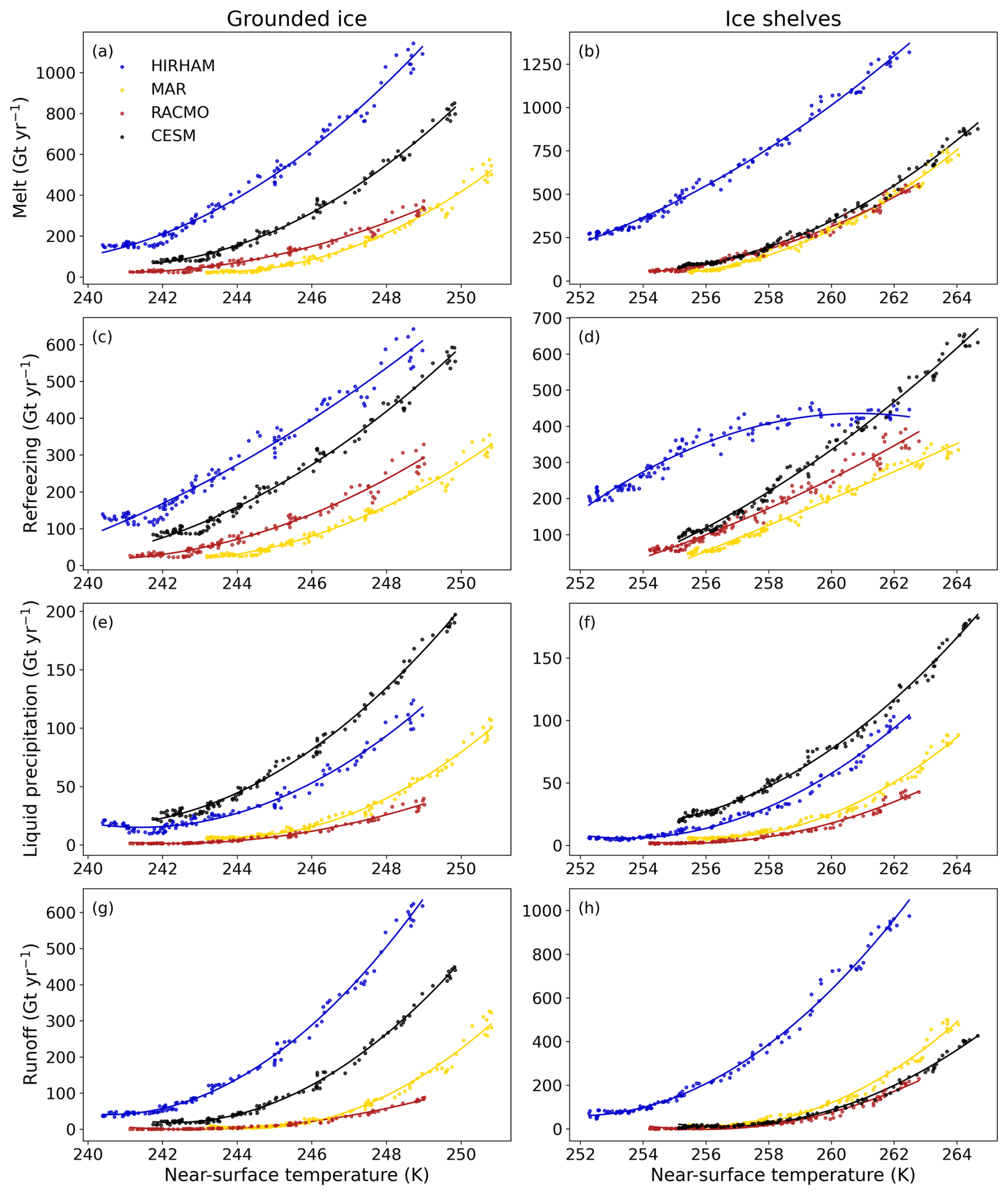
Figure 7 Absolute melt (a, b), refreezing (c, d), liquid precipitation (e, f), and runoff (g, h) in Gt yr⁻¹, as function of the absolute annual near-surface air temperature in K. For the models MAR (yellow), HIRHAM (blue), and RACMO (red) driven by CESM2 (black) under the SSP5-8.5 scenario. Values are integrated over grounded (left) and floating (right) parts of the ice sheet. Note that the y axis scales differ between grounded and floating ice due to the difference in surface areas. A 5-year running mean is applied for clarity.

MAR and RACMO are closely aligned in both their melt and refreezing rates over the reference period (Table S1) and in their evolution with temperature (Fig. 7). Because melt rates are comparable at a given temperature, the near surface temperature offset leads MAR to reach stronger melt than RACMO at the end of the simulation, with projected temperatures of 263.2±0.5 and 261.9±0.4 K, respectively, corresponding to differences of 171 Gt yr⁻¹ over the ice shelves and 150 Gt yr⁻¹ over the grounded ice. Refreezing in the two models evolves in parallel, but is shifted in temperature (2 °C over grounded ice and 1.3 °C over the shelves). This shift translates into differences in refreezing for the same melt rate and therefore contribute to the divergence in runoff between MAR and RACMO (Fig. 7h). This divergence is further amplified by structural differences in the firn representation: the higher retention capacity prescribed in MAR (5 % vs. 2 % in RACMO) partly compensates for its thinner firn, while the initially warmer MAR snowpack likely limits refreezing efficiency regardless of firn air content. In addition, lower snowfall accumulation over the ice shelves in MAR reduces firn renewal, and enhanced rainfall associated with warmer conditions further promotes runoff.

For CESM2, the projected melt evolution over the ice shelves closely follows that of MAR and RACMO. Its similarity to MAR in terms of near surface temperature (Fig. 5) translates into comparable future melt anomalies, with a difference of only 91 Gt yr⁻¹, which is on the same order as their interannual variability 84 Gt yr⁻¹ for MAR and 86 Gt yr⁻¹ for CESM2. Over the grounded ice, CESM2 projects a stronger melt increase, akin to HIRHAM. However, CESM2 predicts persistent and substantial refreezing that continues to grow without reaching a plateau, thereby limiting the acceleration of runoff. In addition, CESM2 exhibits an integrated runoff component evolution over the entire ice shelves that is remarkably similar to MAR and RACMO, despite its native resolution of 110 km.

Although liquid precipitation represents only a small fraction of the total liquid water (melt + rainfall) at the surface, accounting for 8 % in HIRHAM, 10 % in MAR, 7 % in RACMO, and 17 % in CESM2 in future anomalies (Table 3), the models exhibit divergent rainfall rates for similar near-surface temperatures, with HIRHAM and CESM2 producing substantially higher rates than MAR and RACMO for a given temperature (Fig. 7). However, HIRHAM shows an evolution comparable to MAR, reaching similar mean (2080–2099) liquid precipitation rates of 78±15 and 66±12 Gt yr⁻¹ over the ice shelves, and 83±17 and 77±16 Gt yr⁻¹ over grounded ice, respectively. This indicates that liquid precipitation does not contribute to the runoff divergence between HIRHAM and MAR. As for MAR and RACMO, they again display a very similar rainfall–temperature relationship (Fig. 7e and f). Nevertheless, the temperature offset between MAR and RACMO results in higher rainfall rates in MAR by the end of the simulation compared to RACMO (27±7 Gt yr⁻¹ over grounded ice and 33±7 Gt yr⁻¹ over the ice shelves), contributing to their runoff differences. The high liquid precipitation rates reached by CESM2 (171±20 and 160±17 Gt yr⁻¹) explain its similarity in runoff compared to MAR, despite much greater refreezing rates in CESM2 (Fig. 7c and d) and very similar melt rates (Fig. 7a and b). This high estimated liquid precipitation in CESM2 has already been reported by McIlhattan et al. (2020), who identified a systematic rainfall bias in the model. While rainfall remains a relatively small contributor overall compared to surface meltwater production (Donat-Magnin et al., 2020), it nonetheless affects the surface hydrological regime and hence runoff by adding liquid water to the surface.

This surface hydrological regime can be described by the ratio of surface liquid water (melt plus rainfall) to net accumulation (snowfall minus sublimation), defined in the literature as the Melt Over Accumulation (MOA) ratio (Pfeffer et al., 1991; Donat-Magnin et al., 2020; Van Wessem et al., 2023). Theoretical considerations suggest that, when MOA exceeds 0.7, that is, when liquid water input at the surface reaches 70 % of net accumulation, the snowpack can no longer retain and renew pore space, triggering runoff and/or melt-pond formation, thereby increasing the risk of ice-shelf disintegration via hydrofracturing.

Figure 8 shows the integrated surface liquid water and net accumulation over grounded ice (left panel) and ice shelves (right panel). Two distinct regimes emerge over ice shelves: HIRHAM undergoes a much earlier transition than the other models. While its simulated accumulation remains comparable to the other RCMs, excess rainfall and melt push HIRHAM beyond the threshold as early as 253.4±0.5 K, several degrees earlier than MAR, RACMO, and CESM2 (259.9±0.4, 260.7±0.6, and 259.2±0.4 K, respectively) represented by the vertical dotted lines in Fig. 8 (integrated MOA in Fig. S5). This is particularly striking, as HIRHAM's mean temperature during the reference period (1995–2014), is 253.2±0.7 K. This suggests an unrealistically early onset of runaway runoff in HIRHAM, unlike in the other models, where melt and accumulation remain more balanced, making such a scenario far less likely. We also note that over ice shelves, MAR simulates lower accumulation than RACMO (by about 86 Gt yr⁻¹). For comparable melt rates, this reduced accumulation causes MAR to reach the threshold at lower temperatures than RACMO, thereby promoting runoff. In contrast, this threshold is not reached over the integrated grounded ice, despite the large accumulation.

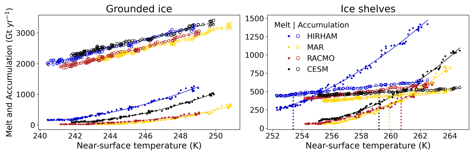
Figure 8 Absolute values of liquid water (melt + rainfall, filled dots) and accumulation (snowfall − sublimation, open circles), expressed in Gt yr⁻¹, as a function of the absolute annual near-surface air temperature in K. For the models MAR (yellow), HIRHAM (blue), and RACMO (red) driven by CESM2 (black) under the SSP5-8.5 scenario. The respective vertical dotted lines indicate the temperature at MOA=0.7. Values are integrated over grounded (left) and floating (right) parts of the ice sheet. Note that the y axis scales differ between grounded and floating ice due to the difference in surface areas. A 5-year running mean is applied for clarity.

The spatial distribution of the temperature anomalies at which the MOA threshold of 0.7 is reached further supports this interpretation (Fig. 9). HIRHAM stands out by reaching the threshold at near-zero or even negative temperature anomalies, indicating that this critical state exposing ice shelves to a risk of destabilization already occurs during or even before the reference period across most ice shelves (Fig. S6). In contrast, MAR, RACMO, and CESM2 show broadly consistent threshold anomalies, with only localized differences – particularly over the Filchner–Ronne and Ross ice shelves-likely reflecting spatial variations in accumulation and melt intensity among the models. Despite these local discrepancies, a coherent pattern emerges over key regions such as the Amery and Larsen ice shelves, where the threshold corresponds closely to the mean temperature of the reference period. This agreement is consistent with observations from the Amery Ice Shelf which experiences intense surface meltwater ponding (Spergel et al., 2021), as well as the Larsen sector where successive collapses of ice shelves – interpreted as being linked to enhanced surface melt – were documented between 1995–2020 (e.g. Rack and Rott, 2004; Willie et al., 2022; Scambos et al., 2009, 2004).

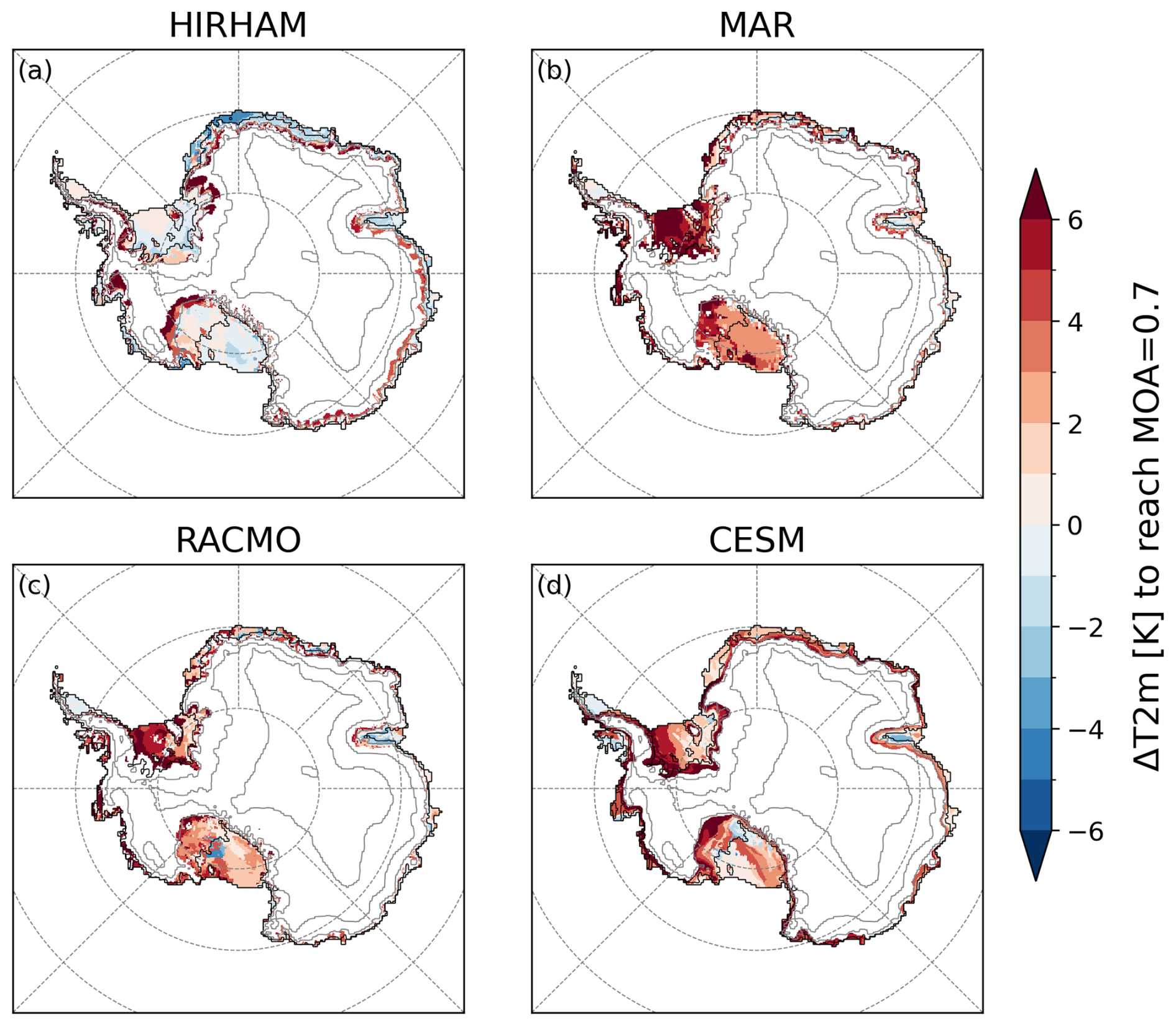
Figure 9 Near-surface temperature anomaly in K, at each grid point when the Melt-over-Accumulation ratio reaches the threshold of 0.7 (MOA=0.7). For HIRHAM (a), MAR (b), RACMO (c), and CESM2 (d) under the SSP5-8.5 scenario. MOA values are calculated using a 5-year running mean.

4 Summary and conclusion

In this study, we investigated the causes of inter-model variability in projections of the Antarctic SMB until the end of the 21st century through a comparative analysis of three RCMs – MAR, RACMO, and HIRHAM – and their common driving ESM, CESM2 under the high-emission SSP5-8.5 scenario. In addition to ESMs, RCMs, thanks to their finer resolution and detailed physics specifically adapted to polar regions, are considered useful complementary tools for producing SMB projections and providing atmospheric forcings to ice sheet models. The inter-model variability revealed here emphasizes the need for continued evaluation and intercomparison of regional models to better constrain uncertainties in SMB projections. Despite identical boundary conditions, the projected SMB strongly diverges over the ice shelves: HIRHAM simulates a strong decline of $-\mathrm{529}\pm \mathrm{72}$ Gt yr⁻¹, MAR a more moderate loss of $-\mathrm{209}\pm \mathrm{58}$ Gt yr⁻¹, while RACMO maintains a near-equilibrium SMB of $+\mathrm{25}\pm \mathrm{19}$ Gt yr⁻¹. These differences mainly stem from the spread in meltwater runoff anomalies: $+\mathrm{775}\pm \mathrm{94}$ Gt yr⁻¹ for HIRHAM, $+\mathrm{390}\pm \mathrm{76}$ Gt yr⁻¹ for MAR and $+\mathrm{170}\pm \mathrm{37}$ Gt yr⁻¹ for RACMO. CESM2 also departs from the three RCMs, projecting a SMB decrease of $-\mathrm{118}\pm \mathrm{36}$ Gt yr⁻¹ driven by a runoff increase of $+\mathrm{329}\pm \mathrm{59}$ Gt yr⁻¹ (Table 4). In contrast, over the grounded ice sheet, inter-model variability remains limited, with similar SMB anomalies ($+\mathrm{610}\pm \mathrm{69}$ Gt yr⁻¹ for HIRHAM, $+\mathrm{757}\pm \mathrm{85}$ Gt yr⁻¹ for MAR, $+\mathrm{870}\pm \mathrm{93}$ Gt yr⁻¹ for RACMO, and $+\mathrm{657}\pm \mathrm{80}$ Gt yr⁻¹ for CESM2), mainly driven by increased snowfall while runoff remains relatively less significant.

A key source of uncertainty lies in the representation of present-day melt rates: within our ensemble, HIRHAM simulates melt and refreezing rates several times higher than MAR and RACMO, which shows closer agreement under current conditions (Fig. 2, Table 3, and Fig. 7a and b). This overestimation is further illustrated in Sect. 3.1.2, where HIRHAM produces 3.5 times more Cumulative Melting Surface than SSM/I observation (Fig. 2 and Table 3). The present-day melt rate governs the nonlinear temperature–melt relationship, and thus the magnitude of future runoff and SMB anomalies. The potential melt bias in HIRHAM during the reference period, and its contemporary melt rates comparable to those projected by MAR and RACMO at the end of the century, certainly accounts for this model divergence which is particularly pronounced under the high-emission scenario SSP5-8.5, amplifying the uncertainty surrounding the extent of projected changes. Although the divergence in HIRHAM melt rates is most striking over ice shelves, the same tendency toward excessive melt or an overly strong temperature sensitivity is also present over grounded ice, where it is partly masked by a larger concurrent increase in snowfall that still dominates SMB changes. The combination of high surface liquid water production and elevated refreezing rates already during the contemporary period, both contributing to enhance the melt–albedo feedback and limit additional firn retention capacity, accounts for the much stronger intensification of runoff in HIRHAM over the ice shelves compared with the other models. As a result, HIRHAM crosses the MOA threshold for meltwater ponding much earlier, amplifying runoff and increasing the vulnerability of ice shelves to hydrofracture-induced destabilization. Notably, most ice shelves in HIRHAM already exceed this threshold during the reference period (Fig. 9).

For MAR and RACMO, although they simulate similar melt and runoff rates under present-day conditions, their projections diverge by the end of the century: runoff anomalies over the shelves reach $+\mathrm{390}\pm \mathrm{76}$ Gt yr⁻¹ in MAR compared to $+\mathrm{170}\pm \mathrm{37}$ Gt yr⁻¹ in RACMO (Table 4). This divergence arises from two factors: (1) difference in surface liquid water production, when toward the end of the simulation MAR produces more liquid water than RACMO owing to systematically higher near-surface temperature; and (2) differences in refreezing rates when, for a given temperature, MAR refreezes less than RACMO. In addition, lower accumulation over the ice shelves in MAR reduces firn renewal, further promoting runoff. Despite these differences, the two models remain broadly consistent in their overall behavior. In CESM2, refreezing remains substantial, yet the increased occurrence of surface liquid water is not sufficiently balanced, leading to a projected runoff increase of $+\mathrm{329}\pm \mathrm{59}$ Gt yr⁻¹ over the shelves – comparable in magnitude to MAR.

Remarkably, CESM2, despite its coarse resolution and its design as an Earth System Model rather than a polar-oriented one, performs comparably to the regional models. This reflects the substantial efforts made to improve the representation of ice-sheet surfaces in CESM2/CLM, which have helped narrow the gap between global and regional models in simulating ice-sheet surface mass balance.

The melt rates produced by HIRHAM at the beginning of the simulation cannot be fully explained with the available model outputs. There is no direct link between high surface energy fluxes and the simulated melt rates, nor can the melt trends be attributed to low albedo values at the beginning of the simulation (Fig. S4). Differences in how HIRHAM translates large-scale warming into local surface conditions were ruled out as a potential explanation, since its projected 500 hPa temperature closely matches that of the other models (Fig. S7). This suggests that other factors inherent to the model physics may contribute, including the model-specific melt–albedo feedback, treatment of water and the absence of feedback with atmosphere (e.g. cooling of the near-surface air during surface melt due to the consumption of latent heat, or conversely, enhanced warming of the near-surface air through sensible heat transfer when surface temperatures increase following albedo reduction after melt).

Other factors likely contribute to the divergences observed in regional projections, particularly in the representation of firn structure and the parameterizations governing meltwater production, retention, refreezing, and runoff. This is well illustrated by RACMO and MAR, which simulate nearly identical present-day melt rates under CESM2 forcing (Table 3) yet differ by close to an order of magnitude in runoff. A thinner firn column, such as the 20 m used in MAR compared with at least 30 m in RACMO, would normally reduce pore volume and retention potential; however, this is more than offset by MAR's higher prescribed maximum water retention capacity (5 % vs. 2 % in RACMO), such that MAR's total retention capacity remains roughly twice that of RACMO across a range of plausible firn density profiles. Firn thickness and retention capacity alone therefore cannot explain the higher runoff in MAR. Instead, this discrepancy primarily reflects two mechanisms. First, MAR's warmer present-day climate produces substantially more liquid water from both melt and rain, which saturates available pore space and depletes firn air content faster than in RACMO regardless of the higher retention threshold. Second, the two models differ in how runoff initiates at ice lenses: MAR permits a fraction of percolating meltwater to run off once it encounters an ice lens or impermeable layer, whereas RACMO requires the entire firn column to reach its irreducible water content before runoff occurs – a structural difference that likely contributes substantially to the higher runoff simulated by MAR at comparable melt rates. This effect may be further amplified by the initial snowpack configuration in this MAR version (MARv3.11), in which ice was present at depth over the ice shelves from the start of the simulation – a choice not retained in more recent model versions – potentially providing additional impermeable layers that favor fractional runoff from an early stage. Beyond this pair, other model-specific choices further shape the ensemble spread: HIRHAM employs a Darcy-flow percolation scheme, whereas the other models use simplified bucket-scheme approaches, leading to different rates of change in firn retention capacity and pore-space depletion. Under dry conditions, differences in firn densification schemes determine how quickly firn air content decreases, while differences in the prescribed density of newly deposited snow affect how effectively fresh snowfall can renew firn air content. Albedo parameterizations further modulate the melt response to warming: HIRHAM prescribes albedo as a function of surface temperature, whereas the other models incorporate the evolution of snow grain size and/or density, resulting in differing expressions of the melt–albedo feedback. Finally, a potentially significant limitation of the current models lies in their simplified representation, or complete non-consideration, of meltwater ponding on the ice surface. The formation of surface meltwater ponding can substantially reduce the local albedo, leading to enhanced solar absorption and further accelerating melt rates (e.g. Dell et al., 2024), while at the same time, a portion of the ponded water can refreeze, partly offsetting mass loss that would otherwise result from runoff (Goutard et al., 2026).

Finally, we would like to note that after 30 years of service the HIRHAM5 model was retired shortly after these simulations were complete, to be replaced by the HARMONIE-Climate system model (e.g. Verro et al., 2025). These will therefore be the last results published from HIRHAM, but the analysis here shows how important continuous assessment, improvement, development and evaluation of regional climate models is.

A promising way to reduce these structural and parametric uncertainties would be to produce projections initialized with a common firn state, using for instance identical vertical discretization and shared parameterizations, to better isolate differences arising from the models' physical evolution. However, progress is currently limited by the restricted set of available model outputs. More advanced diagnostics of firn evolution and melt–albedo feedbacks would require, at minimum, vertically resolved firn properties (depth/thickness, temperature, liquid water content, and density) down to the close-off density. Providing these outputs in future intercomparison exercises would greatly strengthen model evaluation and help clarify the processes driving divergence among models.

These results highlight the need to continue the development and evaluation of climate models, particularly regarding the key physical processes governing SMB and involving surface hydrology (The Firn Symposium team, 2024). In the meantime, the performance differences in present-day melt identified in this study suggest that uncertainty estimates should also account for model skill, motivating a Bayesian treatment of multi-model ensembles. Together, improving process representation and better accounting for model skill are both needed to constrain uncertainties in estimates of Antarctic ice-sheet contribution to sea-level rise.