Rate-induced tipping of ice sheets due to visco-elastic Earth response under idealized conditions

The future evolution of the West Antarctic Ice Sheet will likely be subject to self-reinforcing and irreversible retreat due to the unfolding of a marine ice sheet instability (MISI). How the stabilizing mechanism of glacial isostatic adjustment (GIA) influences the timing and spatial extent of the present and potential future destabilization of the West Antarctic Ice Sheet is highly uncertain. It is thus increasingly subject of numerical modeling studies that are based on observational data, striving for a more realistic representation of the Antarctic Ice Sheet. Here we employ an ensemble of idealized simulations in a synthetic model setup to systematically investigate how the interaction between ice-sheet dynamics and the visco-elastic response of the solid Earth affect the tipping dynamics of an inherently buttressed, Antarctic-type ice-sheet-shelf system that is perturbed by a very slow change in sub-shelf melting (meltrate change of 1 m yr⁻¹ every 100 000 years, aiming for quasi-equilibrium conditions). Using a “Lingle-Clark” bed deformation model we explore a wide range of solid-Earth structures, finding that the threshold of bifurcation-induced tipping (B-tipping), i.e., the critical meltrate magnitude inferred for the ice sheet in quasi equilibrium, strongly depends on the spatial extent of the solid-Earth response and its characteristic viscous response timescale (spanning several orders of magnitude from ∼10 to ∼100 000 years). Compared to the case of a fixed bed (no bed deformation), the bifurcation point increases for the strongest (East-Antarctic type) Earth structures by at least 60 % (from 0.8 to 1.3 m yr⁻¹) whereas for the weakest (West-Antarctic type) Earth structures the increase is more than one order of magnitude larger.

Due to the different timescales involved in the interplay between the dynamics of the ice sheet and the solid Earth, we find that rate-induced tipping (R-tipping) occurs for half of the ensemble members. That is, a sufficiently fast ramp-up of the basal meltrates triggers a MISI even before the critical forcing threshold of B-tipping would be crossed. In fact, due to R-tipping the effective tipping threshold reduces by up to 40 % with respect to the B-tipping threshold (for representative combinations of the upper-mantle viscosity and the lithosphere thickness). In none of our simulations bed uplift can stop a MISI once it is triggered, due to the very fast rate of self-reinforcing grounding-line retreat down the retrograde bed slope and the associated rapid drop in GL bed elevation. Furthermore, we highlight the occurrence of grounding-line overshoots and demonstrate cases of self-sustaining oscillations between advanced and collapsed ice-sheet states. Once triggered, these oscillations continue perpetually just due to the internal, non-linear interaction between ice-flow and solid-Earth dynamics. Our findings highlight that the lithosphere thickness and the upper-mantle viscosity of the solid-Earth structure underlying a MISI-prone ice sheet can strongly affect its tipping dynamics mediated by the strength and timescale of the GIA feedback that counteracts MISI.

1 Introduction

Over the last three decades the West Antarctic Ice Sheet (WAIS) has been losing mass steadily, dictating Antarctica's contribution to global sea-level rise (accounting for up to 90 % of the total ice loss from the Antarctic Ice Sheet; Rignot et al., 2019; Otosaka et al., 2023). This imbalance is mainly driven by increased basal melting of the ice shelves in West Antarctica's Amundsen Sea sector due to enhanced access of relatively warm Circumpolar Deep Water into the ice-shelf cavities (Jenkins et al., 2018; Rignot et al., 2024). The reduced buttressing effect of the thinning ice shelves led to the speed-up, thinning and retreat of the grounded portions of the regional outlet glaciers (Konrad et al., 2018; Milillo et al., 2022), with Pine Island and Thwaites glaciers contributing by far most to the increase in ice discharge into the ocean (Davison et al., 2023b). Numerical modeling suggests that these observed rapid changes might continue into the future (Reese et al., 2023; Bett et al., 2024), possibly leading to a large-scale disintegration of the WAIS (Favier et al., 2014; Joughin et al., 2014; Feldmann and Levermann, 2015; Sutter et al., 2023; Hill et al., 2024; van den Akker et al., 2025) with the potential to increase global mean sea level by more than 3 m (Bamber et al., 2009; Morlighem et al., 2020) and affect the global climate system substantially on the long term (Swart et al., 2023; Li et al., 2024).

The mechanism underlying a potential WAIS collapse is the so-called Marine Ice Sheet Instability (MISI, Weertman, 1974; Schoof, 2007b): an ice sheet that is grounded on a bed below sea level, which is sloping down in landward direction (retrograde bed slope), is prone to self-reinforcing grounding-line (GL) retreat on the retrograde slope due to the highly nonlinear increase of the ice discharge across the GL with increasing bed depth. An increase of the GL flux thins the upstream grounded portion of the ice sheet, which, in turn, induces further GL retreat, closing the self-accelerating MISI feedback loop (Fig. 1). The buttressing provided by ice shelves that are laterally confined or grounded on topographic highs is an important stabilizing factor in the MISI context (Dupont and Alley, 2005; Matsuoka et al., 2015; Fürst et al., 2016; Reese et al., 2018). Their backforce reduces the GL flux, thus alleviating self-sustained GL retreat with the potential to cause GL stabilization on retrograde slope if buttressing is sufficiently strong (Gudmundsson et al., 2012; Cornford et al., 2020; Feldmann et al., 2024). Observations show that West Antarctica's ice shelves generally have been loosing buttressing strength in the recent past and will likely continue to do so in the near future (Gudmundsson et al., 2019; Wild et al., 2022; Miles and Bingham, 2024).

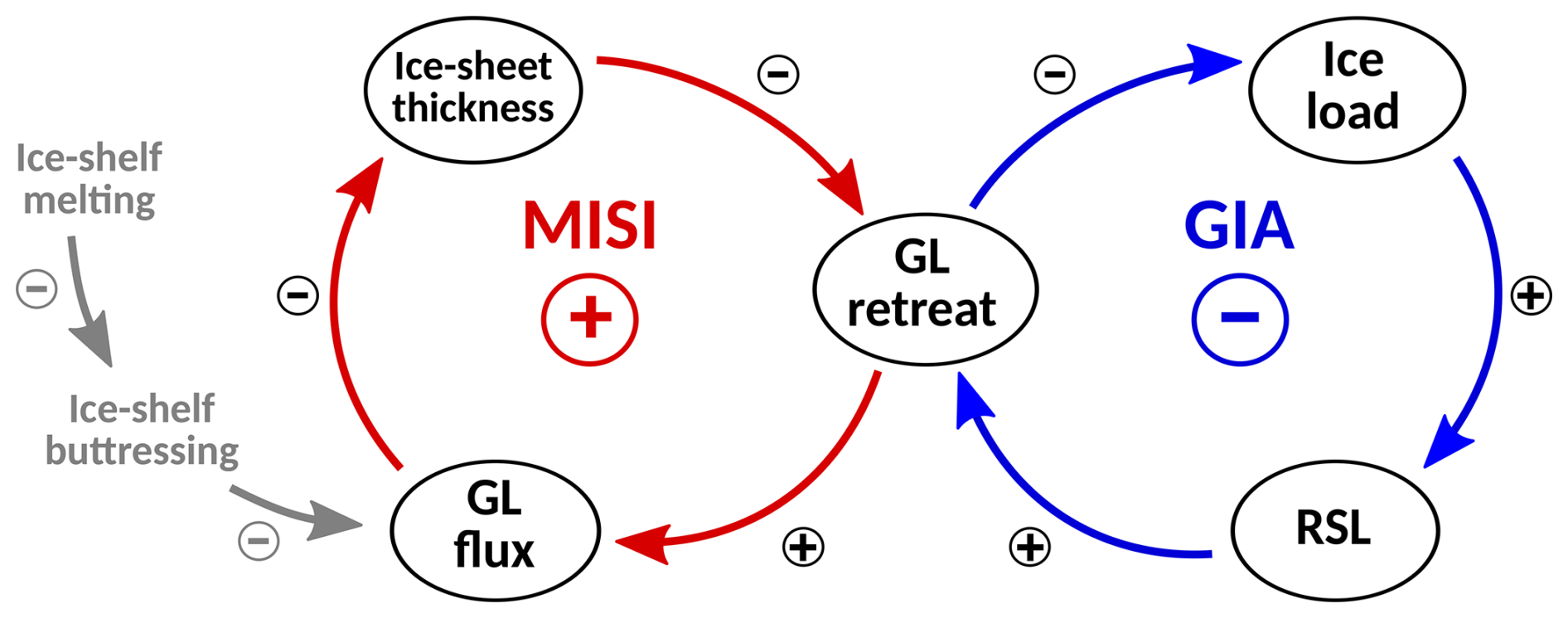
Figure 1 The two main feedback mechanisms, governing the dynamics of the coupled ice-sheet-solid-Earth system. Triggered by basal ice-shelf melting (grey), the self-enforcing MISI feedback (red) promotes GL retreat on retrograde bed and leads to ice-sheet collapse if ice-shelf buttressing is weak enough. Conversely, the dampening GIA feedback (blue) hampers GL retreat and thus counteracts ice-sheet collapse. RSL stands for relative sea level.

Besides ice-shelf buttressing, the process of glacial isostatic adjustment (GIA) is another major stabilizing factor with potentially strong impact on the occurrence, timing and extent of a MISI (e.g., Gomez et al., 2012; Adhikari et al., 2014; Konrad et al., 2015; Barletta et al., 2018; Larour et al., 2019; Kachuck et al., 2020; Book et al., 2022; Albrecht et al., 2024; Gomez et al., 2024; van Calcar et al., 2025; Han et al., 2025): ice-sheet retreat reduces the ice load on the solid Earth which lifts up in response, decreasing the ocean depth (relative sea level) and thus reducing GL flux which hampers GL retreat (Fig. 1). The strength of this stabilizing GIA feedback depends on the structure of the solid Earth, which determines the timescale as well as the horizontal extent and the vertical magnitude of the bed uplift (Gomez et al., 2015; Konrad et al., 2015; Coulon et al., 2021). Observations suggest that West Antarctica's solid-Earth structure is comparatively weak, i.e., it is characterized by an upper-mantle of low viscosity with a thin lithosphere on top, leading to a fast and localized solid-Earth response to ice-load changes, respectively. In contrast, the Earth structure beneath the East Antarctic Ice Sheet is generally found to be much stronger (relatively high upper-mantle viscosity and lithosphere thickness), resulting in a slower and less localized response (e.g., Ritzwoller et al., 2001; Lloyd et al., 2020; Wiens et al., 2023; Hansen and Emry, 2025). Note that strong lateral variations in the solid-Earth structure exist in both East and West Antarctica (e.g., Chen et al., 2018; Lloyd et al., 2020; Hansen and Emry, 2025). Long-term projections of the evolution of the Antarctic Ice Sheet show that West Antarctica's relatively weak solid-Earth structure may substantially delay or even prevent potential future collapse of the WAIS, while East Antarctica's generally stronger solid-Earth structure has a much more limited stabilizing effect on MISI-driven retreat (e.g., Coulon et al., 2021; Gomez et al., 2024; van Calcar et al., 2025; Han et al., 2025). More precisely, it has been found that accounting for the effect of a realistic solid-Earth structure in the projections can delay West Antarctic GL retreat by decades to centuries, reducing Antarctica's sea level contribution by 10 % to 40 % over the coming centuries (Kachuck et al., 2020; Gomez et al., 2024; van Calcar et al., 2025; Han et al., 2025). Furthermore, incorporating solid-Earth feedbacks can have a larger effect on the results than the choice of the climate model used to force the ice-sheet model (van Calcar et al., 2025; Han et al., 2025). It has also been shown that the effect of bed uplift in delaying GL retreat and sea-level rise is most pronounced under low-emission scenarios, while the stabilizing effect of bed uplift is too slow under high-emission scenarios that drive comparatively fast ice-sheet retreat (Gomez et al., 2024).

The triggering of a MISI is typically associated with bifurcation-induced tipping (B-tipping), meaning that an ice sheet in equilibrium transitions abruptly and irreversibly from an advanced stable state to a retreated (collapsed) stable state once the control parameter (e.g., basal ice-shelf melting) crosses a critical threshold (Schoof, 2007a; Rosier et al., 2021). As proposed by Swierczek-Jereczek et al. (2026), the existence of two timescales of (1) ice-sheet retreat and (2) bed response potentially gives rise to a possible rate dependency of MISI initiation, i.e., the occurrence of rate-induced tipping (R-tipping; Ashwin et al., 2012; Wieczorek et al., 2023)¹. This means that a sufficiently fast increase of the control parameter that drives the retreat of a MISI-prone ice sheet could trigger the collapse of the ice sheet at a forcing level that is below the system's bifurcation point, thus lowering its effective tipping threshold. The potential occurrence of R-tipping can be expected to be influenced by both solid-Earth parameters mentioned above: (1) the upper-mantle viscosity, which is proportional to the response timescale of the solid Earth and (2) the lithosphere thickness, affecting the localization of the solid-Earth response and thus also the rates of vertical bed displacement. Rates of anthropogenic global warming are rising and exceed pre-industrial records of temperature change by orders of magnitude (Marcott et al., 2013; Foster and Rahmstorf, 2026), threatening the stability of the Greenland and Antarctic ice sheets also due to the potential occurrence of rate-induced tipping. R-tipping has been examined in the context of the Antlantic Meridional Overturning Circulation as well as in ecological models in several studies (Siteur et al., 2016; Lohmann and Ditlevsen, 2021; Ritchie et al., 2023; Feudel, 2023; Klose et al., 2024; Chapman et al., 2024). To our knowledge, however, so far only one study exists in which R-tipping has been investigated in the MISI context (Swierczek-Jereczek et al., 2026). This study examined the regional (R-)tipping dynamics of the Antarctic Ice Sheet, involving quasi-equilibrium warming experiments, based on a realistic representation of the present-day state of the ice sheet and its dynamics as well as the solid Earth, the ocean and the atmosphere. This approach in particular allowed to infer potential regional R-tipping thresholds accounting for the complexity of an Antarctic real-world setup and the involved dynamics. However, further studies of the R-tipping dynamics of ice sheets and the underlying physical mechanisms are still lacking.

Here we follow a simplified, yet physically reasonable approach to systematically investigate the first-order interaction between ice-sheet and solid-Earth dynamics of a buttressed, MISI-prone outlet glacier. The reduced complexity of the coupled system allows us to focus on the principal physical mechanisms underlying (R-)tipping dynamics, isolated from unwanted interference with potential second-order effects that would occur in more complex model setups. Though strongly idealized, our modeled outlet glacier resembles characteristics of Antarctica's fast flowing ice streams that feed an ice shelf, such as Pine Island or Thwaites glaciers. Sampling a wide range of solid-Earth structures (from very weak to very strong) in a simple “Lingle Clark” visco-elastic bed deformation model (not accounting for lateral variations in the Earth structure) we systematically examine how bed deformation affects the tipping dynamics of such an idealized outlet glacier. That is, we conduct an ensemble of hysteresis simulations forced by a very slow sub-shelf melt forcing ramp-up (ramp-down) that leads to the tipping of the outlet glacier, i.e., triggering irreversible, MISI-driven retreat (re-advance). Inferring the associated critical B-tipping thresholds, we then analyze how the different solid-Earth structures affect the bistability regime of the system. Another major focus of this study is the investigation of the potential occurrence of R-tipping.

2 Methods

2.1 Numerical model

To simulate the coupled evolution of the ice-sheet-shelf system and the solid Earth we use the open-source Parallel Ice Sheet Model (PISM; Bueler and Brown, 2009; Winkelmann et al., 2011). Ice flow is computed using a superposition of the shallow-ice approximation (SIA; Morland, 1987) and the shallow-shelf approximation (SSA; Hutter, 1983) of the Stokes stress balance (Greve and Blatter, 2009). In particular, the SSA allows for stress transmission across the GL and therefore accounts for the buttressing effect of ice shelves that are laterally confined (Gudmundsson et al., 2012; Fürst et al., 2016; Reese et al., 2018) and/or in contact with a pinning point (Favier et al., 2012; Matsuoka et al., 2015; Wild et al., 2022; Feldmann et al., 2024). The model applies a linear interpolation of the freely evolving GL and accordingly interpolated basal friction (Feldmann et al., 2014). GL migration has been evaluated in the model intercomparison exercises MISMIP3d (Pattyn et al., 2013; Feldmann et al., 2014) and MISMIP+ (Asay-Davis et al., 2016; Cornford et al., 2020). To improve the approximation of driving stress across the GL, the surface gradient is calculated using centered differences of the ice thickness across the GL (Reese et al., 2020). All experiments described below are carried out on a regular horizontal grid of 2 km resolution, serving as a compromise between accuracy and computational demand of the simulations (see Fig. A3 and Sect. B for a comparison of results using grids of 1, 2 and 4 km resolution). Note that, however, to achieve convergence of the results with finer resolution the resolution would have to be decreased further, which is not feasible for this study's ensembles of simulations in the light of limited computational capacities and the very long forcing timeseries. The 2 km resolution has been successfully employed for modeling dynamics of fast-flowing ice in similar computational setups in previous studies (e.g., Feldmann and Levermann, 2023).

The response of the solid Earth to ice-load changes is calculated via PISM's built-in “Lingle-Clark” (LC) bed deformation model (Cathles, 1975; Lingle and Clark, 1985; Bueler et al., 2007). The two-layer LC model assumes a Maxwell rheology and is characterized by an Elastic plate Lithosphere that is situated above a half-space representing the Viscous Astenosphere (thus termed ELVA in Swierczek-Jereczek et al., 2024). This modeling approach was originally proposed by Cathles (1975) and Lingle and Clark (1985) applied it to the first time to ice-sheet modeling (Swierczek-Jereczek et al., 2024). The modeled visco-elastic response of the solid Earth to ice-load changes consists of an instantaneous and a time-dependent part. The timescale of the viscous response is a linear function of the prescribed viscosity η of the upper mantle (as shown in Appendix Sect. A1). The thickness of the elastic lithosphere T_e is the second central parameter of the LC model, affecting the spatial distribution of the response. Both parameters neither vary laterally nor radially (in the vertical), i.e., they are spatially uniform, and they are also held fixed in time. The LC model is updated at an interval of 10 model years for all simulations prescribing $\mathit{\eta }\ge \mathrm{5}\times {\mathrm{10}}^{\mathrm{19}}\mathrm{Pa}\mathrm{s}$ (the characteristic viscous solid-Earth response time is at least one order of magnitude larger, see Fig. A1 and Table A1). However, in all simulations that apply the lowest viscosity value the update interval is set to 1 model year in order to account for the very fast timescale response timescale of ≈10 years in this case. No sea-level model is applied, i.e., the height of the sea surface is kept constant in all simulations. Furthermore, rotational effects are neglected in the model.

2.2 Setup and experimental design

2.2.1 Initial bed topography and boundary conditions

Our model setup is designed to simulate the self-reinforcing retreat of an idealized, inherently buttressed Antarctic-type outlet glacier in interaction with the visco-elastic response of the underlying solid Earth. For this purpose we initialize the model with a modified version of the channel-type MISMIP+ bed topography, as used in Feldmann and Levermann (2023, Appendix C), which is held fixed during the model spinup (Fig. 2a). The qualitative shape of the initial bed topography inside the bed trough is as follows (Fig. 2b): along the setup centerline, the bed elevation drops from an inland sill (located at x=0) into an overdeepening (deepest point of the bed depression at x_BD=200 km) and increases towards a coastal sill further downstream (highest point at x_CS=500 km) beyond which the bed elevation drops again (continental shelf break). The initial depth of the overdeepening between x_BD and x_CS is D_BD=900 m (indicated by yellow arrow in Fig. 2b). The resulting average retrograde bed slope of $\mathrm{3}\times {\mathrm{10}}^{-\mathrm{3}}$ (3 m bed elevation change per kilometer in x direction) is on the same order of magnitude as the observed slope steepness of Thwaites Glacier over the same length scale. The bed trough that confines the fast-flowing ice stream (Figs. 2a and S1 in the Supplement) has a width of 160 km, making it similarly wide as Thwaites Glacier's observed fast-flowing trunk at the GL (e.g., Davison et al., 2023a, Fig. 1a).

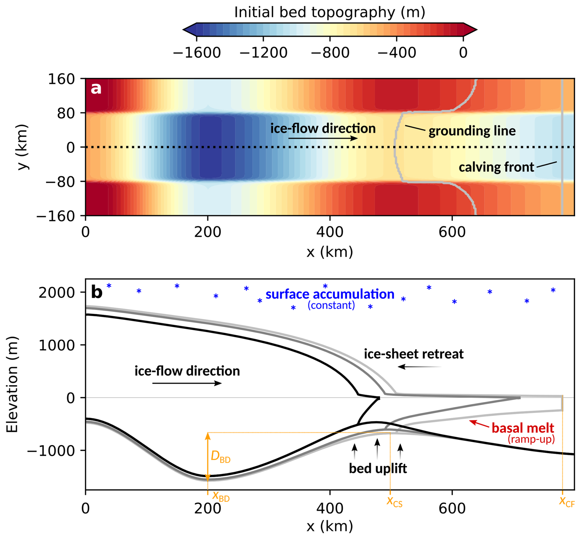
Figure 2 (a) Bed topography (with deep bed depression) prescribed during model spinup with resulting steady-state GL position and fixed calving front (grey contours). (b) Centerline (dotted line in panel a) profiles of bed and ice-sheet-shelf system for different snapshots of a hysteresis simulation (slow ramp-up of basal melt). The initial depth of the bed depression is D_BD=900 m, as indicated by the double-headed yellow arrow.

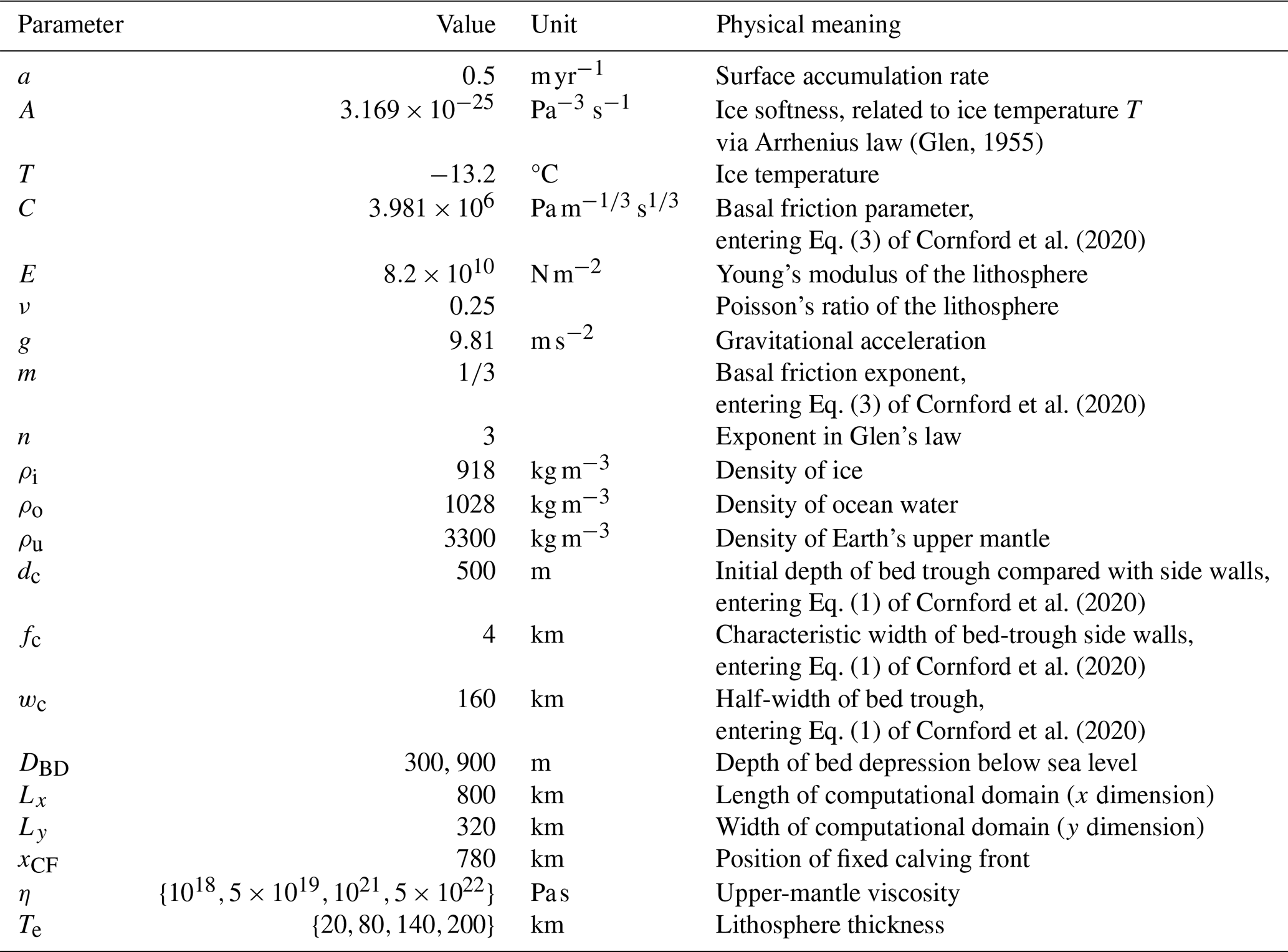
The surface accumulation rate is prescribed as a constant in space and time (see Table 1, also for other parameters). The same applies to the ice softness, i.e., the ice is assumed to be isothermal, neglecting thermomechanical coupling (see Sect. 4 for a discussion of the simplifying assumptions described here). The basal ice-shelf meltrate is spatially uniform, being zero during model spinup while varying in time in subsequent experiments. Basal melting of grounded ice is neglected. Prescribing a spatially and temporally uniform friction coefficient in a Weertman-type friction law (Eq. 3 of Cornford et al., 2020), the resulting basal stresses vary over space and time as part of the non-local SSA stress balance (see Discussion). A single calving condition is applied, where all ice moving beyond x_CF=780 km is calved off. Regarding the lateral margins of the computational ice-sheet model domain, i.e., $y=\pm \mathrm{160}\mathrm{km}$, periodic boundary conditions apply. Note that we avoid prescribing a boundary condition at x=0 by mirroring the setup (including the sub-ice-shelf melt perturbations) along this axis, producing an ice sheet that consists of two symmetric outlet glaciers that share the same ice divide (as we have done in previous studies, e.g., Cornford et al., 2020; Feldmann et al., 2022, 2024). The entire computational ice-sheet model domain thus spans from −800 to +800 km in the x direction. It is centrally embedded into the computational domain of the LC model which is chosen to have 4 times the length of the ice-sheet model domain in both horizontal dimensions (Fig. S13). We refer to this configuration as GSF4 (grid size factor 4). Periodic boundary conditions apply at the edges of the LC model domain and in order to reduce the error that arises from imposing such a boundary condition at finite distance, the model applies a correction to the bed displacement field (Bueler et al., 2007). Test experiments in which we perturb the isostatic equilibrium between spun-up ice sheet and solid Earth by instantaneously removing the complete ice sheet, confirm that this LC model configuration is appropriate for the purposes of this study (see Sect. S1 in Supplement and associated Figs. S13–S15). That is, in these experiments the error in the calculated solid-Earth response arising from the limited size of the LC model domain is small and yields a good compromise with respect to the computational cost of the LC model in comparison to a configuration with a much larger grid size factor of 10 (GSF10) that would completely cover the long-wavelength response. Note that due to the symmetry of our model setup with respect to the ice divide, throughout the study we only consider one of the two outlet glaciers, i.e., the right-hand half of the computational domain (x≥0).

(Glen, 1955)Cornford et al. (2020)Cornford et al. (2020)Cornford et al. (2020)Cornford et al. (2020)Cornford et al. (2020)

Table 1 Physical constants and parameter values as prescribed in the simulations

2.2.2 Model spinup

The spinup starts from a block of ice of 2000 m thickness on the prescribed bed topography. From this initial state an ice-sheet-shelf system evolves that reaches equilibrium after about 30 000 model years. The resulting ice sheet is drained by an ice stream (Fig. S1) through the bed trough, feeding a bay-shaped ice shelf which provides buttressing to the upstream ice. The depth of the initial bed geometry was chosen such that the steady-state GL of the ice stream inside the bed trough is located on the tip of the coastal sill at the end of the spinup (Fig. 2). This way, in the course of the subsequent perturbation experiments, a relatively small increase in basal ice-shelf melting m (from 0 to $\approx \mathrm{1}\mathrm{m}{\mathrm{yr}}^{-\mathrm{1}}$) can push the GL from its stable position towards an unstable position on the retrograde slope, triggering a MISI. Since the deformation of the bed is switched off during the spinup, the resulting steady-state ice sheet can be considered to be in equilibrium with the prescribed bed topography.

2.2.3 Ensemble of solid-Earth structures

The equilibrium obtained from the spinup serves as the initial state for an ensemble of simulations that systematically explores how the configuration of the solid-Earth structure affects the interaction between the dynamics of the ice sheet and the solid Earth. For this purpose, we vary the two central parameters that determine the solid-Earth structure in the LC model, i.e., the upper-mantle viscosity, η, and the lithosphere thickness, T_e (see Table 1). In each simulation both parameters are constant in space and time. Our selection of the parameter values ($\mathit{\eta }=\mathit{\{}{\mathrm{10}}^{\mathrm{18}},\mathrm{5}\times {\mathrm{10}}^{\mathrm{19}},{\mathrm{10}}^{\mathrm{21}},\mathrm{5}\times {\mathrm{10}}^{\mathrm{22}}\mathit{\}}\mathrm{Pa}\mathrm{s}$ and $T_{\mathrm{e}}=\mathit{\{}\mathrm{20},\mathrm{80},\mathrm{140},\mathrm{200}\mathit{\}}\mathrm{km}$) is based on the parameter ranges used by Coulon et al. (2021), liberally covering the observed ranges and the associated uncertainties of these two variables (e.g., Ritzwoller et al., 2001; Whitehouse et al., 2019; Lloyd et al., 2020; Wiens et al., 2023). The parameter space resulting from each combination of the above values of η and T_e (16 combinations in total) in particular captures the weaker Earth structures (low η and T_e values) that are characteristic for West Antarctica, and the stronger Earth structures (high η and T_e values) that are characteristic for East Antarctica. Furthermore, the parameter space represents intermediate solid-Earth structures (medium values of η and T_e) as well as less typical combinations (high values of η combined with low values of T_e and vice versa).

2.2.4 Ramp-up/down (hysteresis) experiments

All 16 members of the solid-Earth parameter space (plus one model realization with a fixed bed) start from the same ice-sheet-shelf system that has been spun up on the same fixed bed topography. In each of these realizations the initial equilibrium is perturbed by basal ice-shelf melting, that, starting from zero, is ramped up at a rate of $\dot{m}={\mathrm{10}}^{-\mathrm{5}}$ m yr⁻² (red line in Fig. 3). The previously fixed bed topography is now free to evolve. The very slow increase in sub-ice-shelf melting (1 m yr⁻¹ every 100 000 years) is intended to let the system evolve in a quasi equilibrium. Note that the forcing rate is reduced by one order of magnitude for all runs with the largest upper-mantle viscosity ($\mathit{\eta }=\mathrm{5}\times {\mathrm{10}}^{\mathrm{22}}\mathrm{Pa}\mathrm{s}$) due to the associated very slow response time of the solid Earth (Table A1). In most cases, the meltrate ramp-up ends at a final value of 5 m yr⁻¹. By then, the ice sheet has collapsed and stabilized. Subsequently, the forcing is reversed, i.e., the meltrate is ramped down at the same slow rate (blue line in Fig. 3). During this ramp-down the ice sheet re-advances and tips back to its original advanced state. In general, the ice-sheet response (e.g. GL migration) to the ramp-up and subsequent ramp-down forms a hysteresis curve (Fig. 4a). In the following, we refer to the GL curve in response to the slow ramp-up (ramp-down) as the forward (backward) branch of the hysteresis curve. Most of the analysis in this study will focus on the forward hysteresis branch, motivated by the observed recent and present-day retreat and potential future collapse of the MISI-prone WAIS.

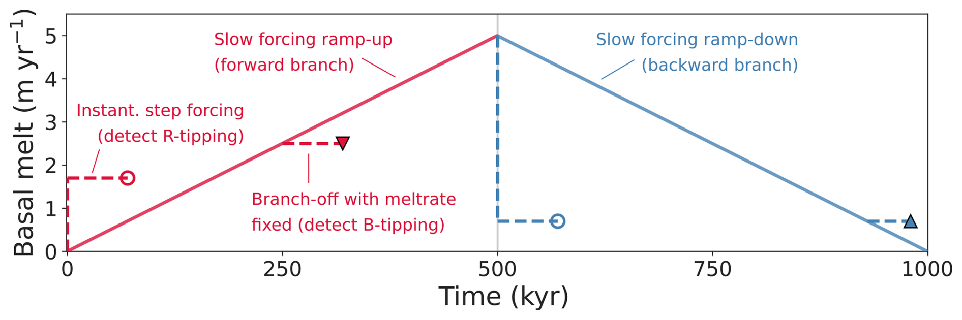
Figure 3 Exemplary forcing timeseries. Slow forcing ramp-up (red) and ramp-down (blue) applied in the hysteresis experiments (Sect. 2.2.4). Branch-off experiments (Sect. 2.2.5), from the ramp-up/ramp-down with the current meltrate held fixed to simulate the associated equilibrium state and infer B-tipping thresholds, are indicated by triangles. Step-forcing experiments (Sect. 2.2.6) that apply an infinitely fast forcing ramp-up/ramp-down to a specific meltrate value in order to check for possible rate-dependency of the resulting steady state to the forcing rate are highlighted by a circle. The resulting hysteresis curve with inferred B-tipping thresholds and R-tipping range are shown in Fig. 4.

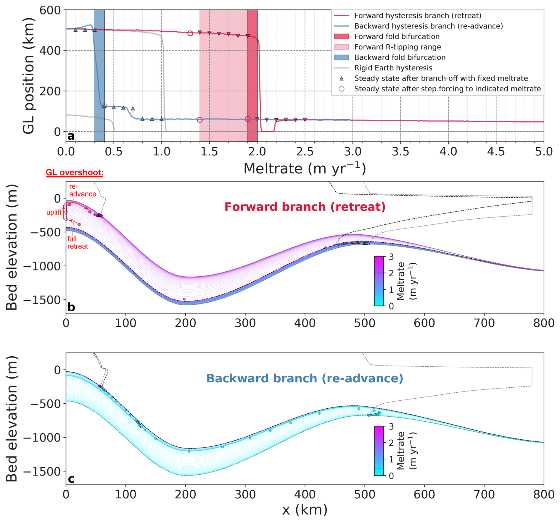
Figure 4 Evolution of GL position, ice and bed profiles in response to the slow ramp-up and subsequent ramp-down of the basal ice-shelf melt forcing (1 m yr⁻¹ per 100 000 model years) with solid-Earth parameters η=10²¹ Pa s and T_e=80 km and an initial bed depression depth of D_BD=900 m. (a) Hysteresis curves of the centerline GL position with red and blue curves representing the forward and the backward branch of the hysteresis, respectively. Red and blue areas give the ranges of B-tipping. Light red area highlights the range of R-tipping. Triangles represent steady states after branching off from the hysteresis curve at fixed melt rate. Circles denote equilibrium states after an instantaneous step forcing to the respective melt rate (see Fig. 3 for the different forcings). Grey curves correspond to the case of a fixed bed. (b) Evolution of the centerline bed topography (1000-year snapshots) during forcing ramp-up with GL position marked by small circles. Dashed contours represent ice-shelf draft and bed profile for initial and final equilibrium state (grey) and the last stable state before collapse (black). The mechanism of GL overshoot is highlighted by the red circles (GL positions) and arrows (direction of GL migration) on the left-hand-side of panel (b): after the GL has fully retreated to x=0, the lagged bed uplift continues and the GL starts to re-advance once the local bed depth is shallow enough to allow for ice-sheet regrowth from the lateral ridges (see corresponding Fig. S9). (c) Evolution of GL and bed during forcing ramp-down, analogous to panel (b) (see corresponding Fig. S10). The B-tipping thresholds are marked by dashed lines in the colorbars.

2.2.5 Branch-off experiments to infer B-tipping thresholds

To infer the critical forcing magnitude at which ice-sheet collapse (or re-advance) occurs, we run simulations that branch off from the hysteresis curve at different meltrates prior to collapse (or re-advance), letting the system run into equilibrium for several 10 000 to 100 000 model years under the respective constant melt rate (red and blue lines with triangle in Fig. 3). For the forward branch of the hysteresis curve (GL retreat), the critical threshold of B-tipping is located between the largest forcing magnitude for which the glacier still stabilizes in its advanced state and the next larger forcing magnitude for which the glacier collapses. The branch-off experiments are also carried out for the backward branch of the hysteresis curve. Here, the critical threshold of B-tipping lies between the smallest meltrate for which the glacier still stabilizes in its collapsed state and the next lower meltrate for which the glacier tips back into the advanced stable regime. The branch-off simulations are sampled at a meltrate interval of 0.1 m yr⁻¹. For simplicity, we will refer to the critical meltrate at which tipping occurs, m_B-tip, as the lowest (highest) meltrate for which the ice sheet collapses (re-grows) in the branch-off experiments.

2.2.6 Step-forcing experiments to detect potential R-tipping

To investigate the potential occurrence of R-tipping for the forward branch of the hysteresis curve, the initial steady state is perturbed by a step forcing to a meltrate level just below the B-tipping threshold for each model realization. That is, the forcing is ramped up from zero to the specific meltrate instantaneously (red line with circle in Fig. 3). If this results in a collapse of the ice sheet, then the model realization exhibits R-tipping due to the fact that a slow ramp-up to the same meltrate does not lead to a collapse. In this case, further step-forcing experiments to lower meltrate levels are conducted to confine the range of R-tipping occurrence associated with the specific model realization. These experiments are carried out analogously for the backward branch of the hysteresis curve (blue line with circle in Fig. 3). Starting from the initial state of the backward branch, the meltrate is instantaneously lowered from the initial value (typically 5 m yr⁻¹) to meltrates above the backward B-tipping threshold in order to check whether the ice sheet tips back into its advanced state for this instantaneous ramp-down (potential occurrence of backward R-tipping).

3 Results

3.1 Hysteresis and involved feedbacks

In all hysteresis experiments, the slow ramp-up of the forcing causes a gradual retreat of the ice sheet's GL onto the retrograde bed slope: the applied melting at the ice-shelf base thins the ice shelf, which reduces its buttressing effect, inducing higher ice discharge across the GL and thinning of the upstream grounded ice sheet, resulting in GL retreat (Figs. 1 and 4a). Since the retrograde bed slope is very shallow in the vicinity of the tip of the costal sill (initial location of the GL; Fig. 2), the destabilizing MISI mechanism of self-reinforcing GL retreat is weak initially (as can be seen in Figs. 4b and 5 from the proximity of the small circles indicating GL positions at 1000-years steps). Thus, in the absence of bed deformation, the buttressing effect of the ice shelf is large enough to stabilize the GL on the shallow retrograde slope for low meltrate magnitudes $m\le \mathrm{0.7}\mathrm{m}{\mathrm{yr}}^{-\mathrm{1}}$ (grey curves in Figs. 4a and 6). For the case of a deformable bed, the bed uplift in response to the decreasing ice load leads to a decrease in the relative sea level, reducing the ice discharge across the GL (stabilizing GIA feedback in Fig. 1), thus allowing stable GL positions farther inland and for higher forcing magnitudes. Depending on the solid-Earth structure and the initial geometry of the bed depression, these forcing magnitudes span a range from $m=\mathrm{1.3}\mathrm{m}{\mathrm{yr}}^{-\mathrm{1}}$ to 18 m yr⁻¹ (Figs. 7 and S5; see Sects. 3.2 and 3.4 for a detailed analysis). In most cases, the MISI becomes dominant when the GL approaches x=400 km. Then the strong increase in GL flux (due to the increase in GL bed-depth in the course of GL retreat) cannot be compensated by the uplifting bed such that the MISI fully unfolds.

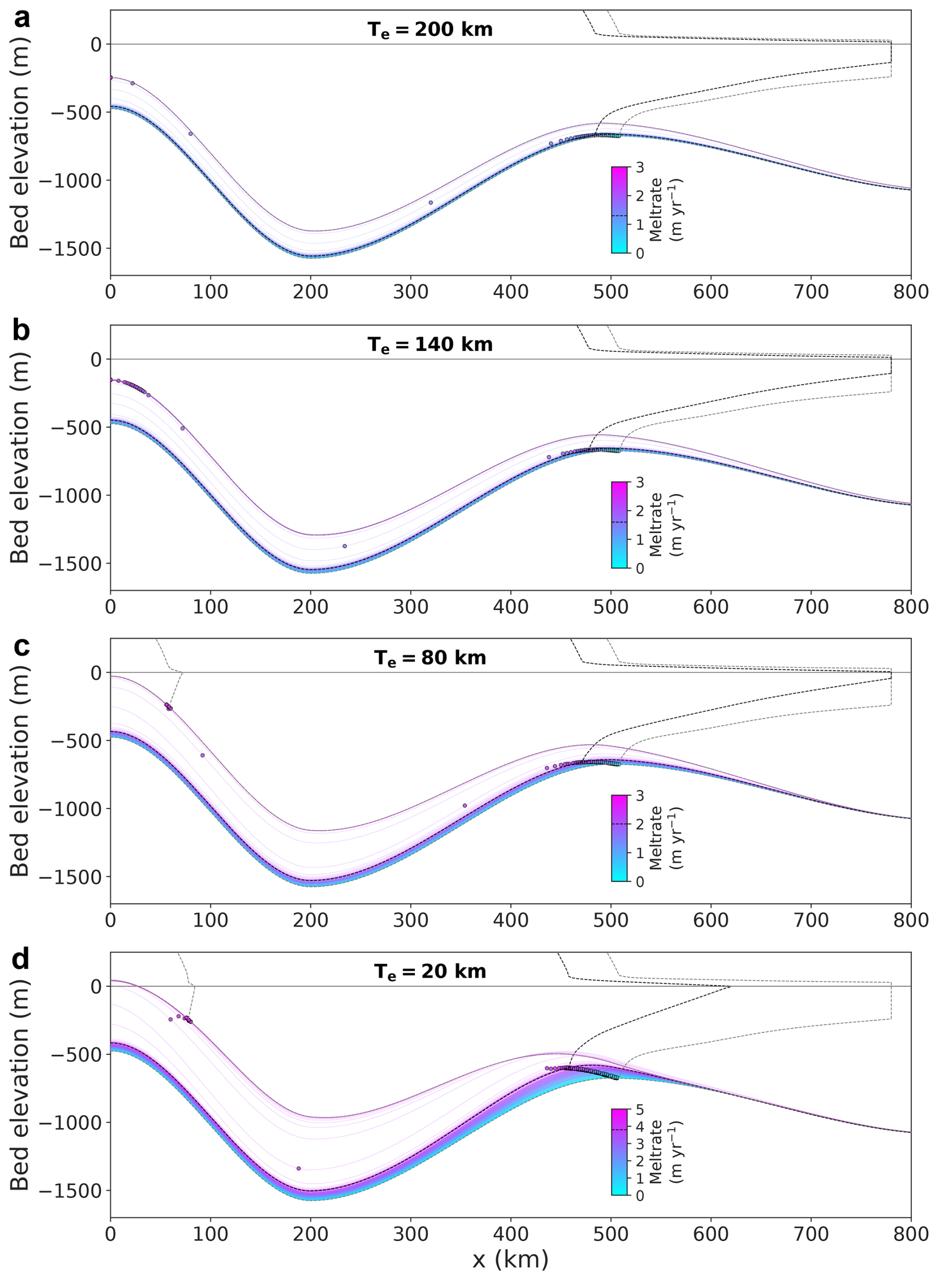
Figure 5 Comparison of the evolution of the centerline bed topography during slow forcing ramp-up for the four applied lithosphere thicknesses, T_e (fixed upper-mantle viscosity $\mathit{\eta }=\mathrm{5}\times {\mathrm{10}}^{\mathrm{19}}\mathrm{Pa}\mathrm{s}$). Profile snapshots have an interval of 1000 yr with GL positions marked by small circles. Dashed contours represent ice-sheet and bed profiles for initial and final equilibrium state (grey) and the last stable state before collapse (black). The B-tipping threshold is marked by a dashed line in the colorbars. Note the increase in the locality of the bed uplift with decreasing lithosphere thickness, i.e., from top to bottom.

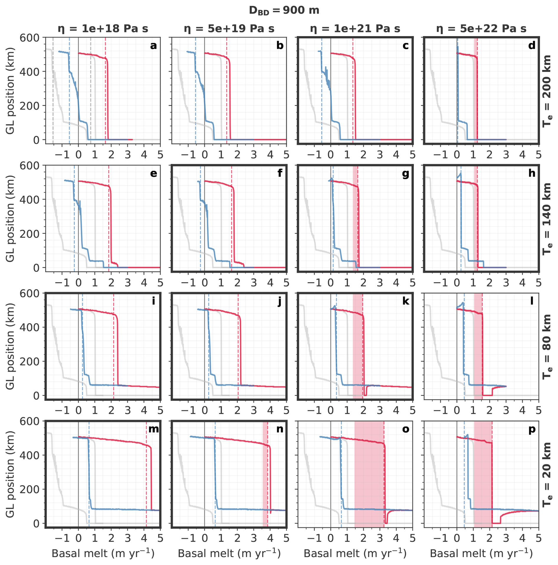
Figure 6 Hysteresis curves of the centerline GL position. Each panel represents one combination of the two solid-Earth parameters η (upper-mantle viscosity; increasing from left to right) and T_e (lithosphere thickness; increasing from bottom to top). Red and blue curves show the quasi-equilibrium trajectories for the slow forcing ramp-up and ramp-down, respectively. Grey curves show the response for a fixed bed. Dashed vertical lines indicate the inferred B-tipping thresholds. Thick-framed panels represent plausible combinations of η and T_e, including weak (West-Antarctic type) solid Earth structures in the bottom left and strong (East-Antarctic type) solid Earth structures in the top right.

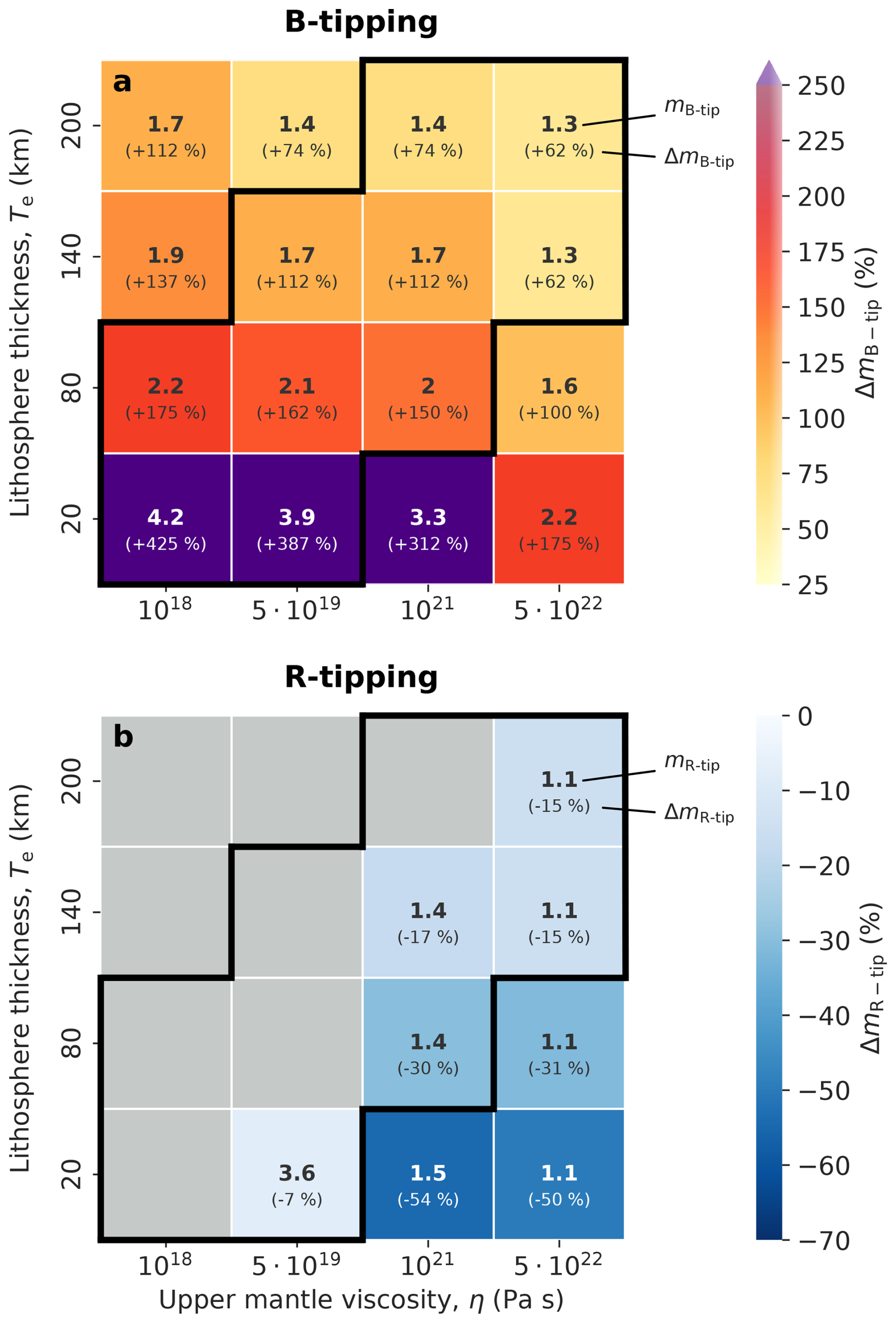
Figure 7 Heat maps showing the shift in the critical meltrate for (a) B-tipping (relative to the threshold of the fixed-bed case, see Eq. 1) and (b) potential R-tipping (relative to the B-tipping threshold, see Eq. 2). The results apply to the case of an initially deep bed depression (D_BD=900 m), for which the reference tipping threshold in the absence of bed deformation is $m_{\text{B-tip,fixed}}=\mathrm{0.8}\mathrm{m}{\mathrm{yr}}^{-\mathrm{1}}$. The absolute values of the respective tipping thresholds, m_B-tip and m_R-tip, are given by bold large numbers and the values of tipping threshold increase relative to the fixed-bed case, Δm_B-tip and Δm_R-tip, are given in brackets (see annotations in panels a and b). Black-framed area highlights the regime of plausible combinations of η and T_e, stretching from weak (West-Antarctic type) solid Earth structures in the bottom left to strong (East-Antarctic type) solid Earth structures in the top right.

As the ice sheet undergoes rapid retreat down the retrograde slope, the GL passes through the bed depression and enters the inland prograde bed section, which acts to stabilize the GL due to the decrease in GL flux with GL retreat. However, a direct stabilization of the GL on the prograde slope only occurs in the presence of a sufficiently weak Earth structure and thus a strong GIA feedback (Fig. 6), i.e., for the combination of a sufficiently localized response (T_e≤80 km) and a sufficiently fast response time ($\mathit{\eta }\le \mathrm{5}\times {\mathrm{10}}^{\mathrm{19}}\mathrm{Pa}\mathrm{s}$). In all other cases, the GL retreats all the way to x=0 such that the ice stream inside the bed trough vanishes (temporarily). Note that throughout this study we consider the locality of the bed response as being characterized by the wavelength and the amplitude of the visco-elastic bed deformation. That is, a more localized bed response goes along with a smaller horizontal extent and a larger vertical magnitude of the bed deformation, respectively. A more localized bed response usually occurs for a thinner lithosphere due to the associated lower flexural rigidity of the lithosphere (e.g., Gomez et al., 2012; Konrad et al., 2015; Coulon et al., 2021). This can be seen from Fig. 5 where, with increasing lithosphere thickness from bottom to top, the response becomes more widespread, i.e., the bed uplift is less pronounced under the shrinking ice body but reaches farther out downstream of the GL. This difference in the response pattern is illustrated in more detail (in plan view) in Figs. S13 and S14 (for more details see Sect. 1 of the Supplement): in the case of the thinnest lithosphere (T_e=20 km) the bed displacement is comparatively strong under the ice body but spreads at maximum twice the ice body's width in the horizontal (Fig. S14a). In contrast, for the thickest lithosphere (T_e=200 km), the vertical displacement is weaker in magnitude but spreads about nine times the ice-sheet width in the horizontal dimension (Fig. S14b).

Several model realizations show an overshoot of the GL, i.e., after retreating to x=0 the GL re-advances in response to the delayed bed uplift (see Sect. 3.5). For very widespread responses (thick lithospheres, T_e≥140 km) the GL does not re-advance at all (Fig. 6a–h). Irrespective of the occurrence of GL overshoot, thinner lithospheres generally promote GL stabilization further downstream due to the stronger locality of the bed response (stronger bed uplift in the vicinity of the inland sill).

In the course of ice-sheet retreat, collapse and stabilization, the bed elevation overall increases by several hundreds of meters in the previously grounded area compared to the initial state (Fig. 4b). The bed uplift is most pronounced in the region of the bed depression, i.e., the region of the initially thickest ice (local uplift of up to nearly 700 m; Fig. 5). As a consequence, the retrograde bed slope flattens (Figs. 4b and 5). The ramp-down of the forcing then causes a slow regrowth of the ice sheet as the ice shelf thickens and thus provides more buttressing. The advance of the ice sheet goes along with bed subsidence due to the increasing ice load (Fig. 4c), hampering GL advance. However, at some stage the basal-melt forcing has decreased sufficiently such that the thickened ice shelf provides enough buttressing to induce GL advance onto the retrograde bed section. At this point GL advance becomes self-reinforcing due to the strong inverse MISI feedback, which outpaces the stabilizing GIA feedback. Eventually, the GL reaches its initial position when the meltrate has been ramped down to zero (initial value). Note that for a solid-Earth response that spreads comparatively wide (T_e≥140 km), GL re-advance towards its initial position can occur in several steps (blue curves in Fig. 6a–f) as opposed to the usual large, single-step event of GL migration after passing the tipping threshold. This is a result of the temporary grounding (pinning) of the thickening ice shelf on the retrograde slope in the course of slowly increasing meltrates. Such temporary grounding has been reported in earlier idealized studies for both MISI-driven ice-sheet retreat (Jong et al., 2018) and re-advance (Feldmann et al., 2024). In our simulations the bed subsidence emerging from the ice-shelf grounding hampers GL re-advance such that the full re-advance occurs for comparatively low (even negative) forcing values.

3.2 B-tipping

The meltrate threshold, m_B-tip, at which the self-reinforcing retreat (MISI) is triggered during the forcing ramp-up strongly depends on the configuration of the solid-Earth structure. The lowest B-tipping value, $m_{\text{B-tip,fixed}}=\mathrm{0.8}\mathrm{m}{\mathrm{yr}}^{-\mathrm{1}}$, is found for the fixed-bed case due to the absence of bed uplift (Fig. 6a, dashed grey line). If the bed is allowed to adjust to ice-load changes, then weaker Earth structures (lower values of the mantle viscosity and/or the lithosphere thickness) generally shift the B-tipping threshold towards higher values (going from the upper right to lower left in Fig. 6). The associated generally faster and more localized bed-uplift rates have a larger effect in diminishing GL ice discharge and thus GL retreat. To express the change in the B-tipping threshold relative to the reference case of a fixed bed, we calculate

$$\begin{array}{}\text{(1)}& \mathrm{\Delta }{m}_{\text{B-tip}}={\displaystyle \frac{m_{\text{B-tip}}-m_{\text{B-tip,fixed}}}{m_{\text{B-tip,fixed}}}}\cdot \mathrm{100}\mathrm{\%},\end{array}$$

with critical B-tipping thresholds of the specific solid-Earth configuration, m_B-tip, and of the fixed-bed case, m_B-tip,fixed (numbers in brackets in Fig. 7a). Thus, a doubling of the B-tipping threshold relative to the fixed-bed case would mean a shift of $\mathrm{\Delta }{m}_{\text{B-tip}}=+\mathrm{100}\mathrm{\%}$. The increase of the B-tipping threshold compared to the fixed-bed case ranges from Δm_B-tip=62 % to 425 % (Fig. 7a). In most cases, the B-tipping threshold is at least doubled and the magnitude of the shift of the threshold increases towards the weakest solid-Earth structures (purple regimes in Fig. 7a), resulting from the strong locality of the response associated with the very thin lithosphere.

In all configurations of the solid-Earth structure, the ice-sheet collapse in response to the forcing ramp-up is irreversible, as the re-advance of the ice sheet during the subsequent forcing ramp-down does not take place on the same path as the retreat (Figs. 4a and 6). In fact, the return of the ice sheet to its advanced state requires a lowering of the forcing magnitude below the threshold of ice-sheet collapse. The resulting hysteresis curve of, e.g., the GL position envelopes a bistability regime in which the ice sheet can be either in its advanced or collapsed state, depending on the forcing history. The size of the bistability range increases for increasing weakness of the solid-Earth structure, resulting from the associated increasing strength of the stabilizing GIA feedback, which shifts the thresholds of (1) collapse to higher values and (2) re-advance to lower values.

3.3 R-tipping

For several configurations of the solid-Earth structure the threshold beyond which self-reinforcing retreat is triggered depends on the rate of the increase in basal ice-shelf melting (R-tipping; red shading in Figs. 4a and 6). In these cases, a sufficiently fast forcing rate induces an ice-sheet collapse at a forcing magnitude that is below the critical threshold of B-tipping (see Movie S1, Feldmann, 2026c). We express the rate-dependent shift in the critical tipping threshold compared to the B-tipping threshold by

$$\begin{array}{}\text{(2)}& \mathrm{\Delta }{m}_{\text{R-tip}}={\displaystyle \frac{m_{\text{R-tip}}-m_{\text{B-tip}}}{m_{\text{B-tip}}}}\cdot \mathrm{100}\mathrm{\%},\end{array}$$

where m_R-tip is the R-tipping threshold for an infinitely fast forcing ramp-up (lower end of the R-tipping regime; see Fig. 4a). For the occurrence of R-tipping, the shift in the tipping threshold relative to the B-tipping threshold ranges from −7 % to −62 % (generally decreasing for thinner lithospheres and larger upper-mantle viscosities; Fig. 7b), indicating an effective reduction of the critical tipping threshold through the occurrence of R-tipping.

Throughout the ensemble, R-tipping occurs for intermediate to high values of η, i.e., for moderate to high strengths of the Earth structure. This can be explained by considering (1) the timescale of the viscous solid-Earth response, τ_SE, which increases linearly with η (see Sect. A1), and (2) the timescale of GL retreat (ice-load change) prior to tipping that would apply in the absence of bed deformation, τ_L,st, which decreases for a higher forcing rate (decreasing ice-shelf buttressing) and for a steeper retrograde bed slope (larger GL flux). In the following we distinguish between three cases to argue under which conditions R-tipping generally occurs (visualized in Fig. 8):

1. Very low mantle viscosity. (no R-tipping, Fig. 8a): the solid-Earth response is very fast compared to the timescale of stable GL retreat (ice-load change), i.e., ${\mathit{\tau }}_{\mathrm{SE}}\ll {\mathit{\tau }}_{\mathrm{L},\mathrm{st}}$ (in the limit case the response would be instantaneous). Thus, the bed adjusts quasi immediately to GL retreat, regardless of the timescale of the forcing. This means that the bed is close to equilibrium with respect to the changing ice load even for a high forcing rate and thus a comparatively fast, stable GL retreat prior to the ice-sheet collapse. Consequently, the threshold of destabilization is independent of the forcing rate.

2. Moderate to high mantle viscosity. (R-tipping occurs, Fig. 8b): the timescale of the solid-Earth response is similar to or slower than the timescale of GL retreat. Under this condition it is possible that the bed is close to equilibrium with respect to the changing ice load for a very low forcing rate (${\mathit{\tau }}_{\mathrm{SE}}<{\mathit{\tau }}_{\mathrm{L},\mathrm{st}}$) but not for a high forcing rate (${\mathit{\tau }}_{\mathrm{SE}}>{\mathit{\tau }}_{\mathrm{L},\mathrm{st}}$). The lagged solid-Earth response to a high forcing rate (and thus faster retreat) leads to ice-sheet destabilization at lower forcing magnitudes (R-tipping threshold) compared to the B-tipping threshold, which holds for a very low forcing rate (and thus slower retreat).

3. Fixed bed. (no R-tipping, Fig. 8c): the solid-Earth does not respond to the ice-load change, i.e. the timescale of the response can be considered as infinitely slow (τ_SE→∞). Thus, regardless of the forcing rate, the GL retreat and bed evolution do not interfere, making the threshold of destabilization independent of the forcing rate.

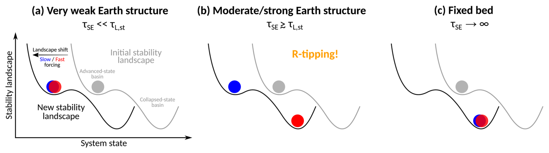
Figure 8 Schematic to illustrate under which conditions R-tipping emerges in our simulations (inspired by Ritchie et al., 2023, Fig. 1). In each panel the grey ball represents the initial steady state of the ice sheet (associated with the grey initial stability landscape) which is perturbed by basal ice-shelf melting (ramp-up forcing that shifts the stability landscape to a new state highlighted in black) with resulting final steady states represented by colored balls (blue for a slow forcing and red for a fast forcing). (a) If the Earth structure is very weak, then the solid-Earth response is quasi-instantaneous and thus, independently of the forcing rate (slow or fast shift of the stability landscape), the system remains in its advanced stable state. (b) For a moderate to strong Earth structure, if the timescale of ice-load change is similar to or faster than the timescale of the solid-Earth response, then the response of the system depends on the forcing rate, i.e., it collapses (remains stable) for a fast (slow) shift of the stability landscape. (c) If the bed elevation is held fixed, then the timescale of the solid-Earth response is infinite and thus the ice sheet will tip into a collapsed state, independently of the forcing rate. All cases assume that the forcing is ramped up to a value that is (1) below the critical B-tipping threshold that is specific to the applied solid-Earth structure, m_B-tip, and (2) above the B-tipping threshold of the fixed-bed case, m_B-tip,fixed.

Note that the locality of the solid-Earth response modulates the pattern of R-tipping occurrence described above: for a given upper-mantle viscosity a more localized bed uplift due to a thinner lithosphere is associated with a higher B-tipping threshold, i.e., a higher critical basal meltrate. Larger basal meltrates and associated stronger ice-shelf thinning reduce the ice-shelf buttressing effect and force the GL into regions of deeper and steeper bed slope. Both effects increase GL discharge rates and thus reduce the timescale of GL retreat (smaller τ_L,st). For instance, in the case of $\mathit{\eta }=\mathrm{5}\times {\mathrm{10}}^{\mathrm{19}}\mathrm{Pa}\mathrm{s}$ the timescale of the solid-Earth response, τ_SE=475 years, is generally faster than the timescale of GL retreat, ${\mathit{\tau }}_{\mathrm{L}}\sim {\mathit{\tau }}_{\mathrm{L},\mathrm{st}}\approx \mathrm{6000}\mathrm{years}$, preventing the occurrence of R-tipping (see Table A1 for more numbers). However, for the thinnest lithosphere, the strong forcing magnitude required to trigger the MISI decreases τ_L,st substantially, leading to a delay in the solid-Earth response (${\mathit{\tau }}_{\mathrm{L},\mathrm{st}}<{\mathit{\tau }}_{\mathrm{SE}}$) that allows for R-tipping (Fig. 6n). This also explains the presence (absence) of R-tipping for a thin (thick) lithosphere in case of η=10²¹ Pa s. For this viscosity value the timescales of stable GL retreat (${\mathit{\tau }}_{\mathrm{L},\mathrm{st}}\approx \mathrm{6000}\mathrm{years}$) and solid-Earth response (τ_SE≈9000 years) are generally roughly similar. However, the smaller tipping thresholds for thicker lithospheres result in timescales of stable GL retreat that are effectively slower (larger τ_L,st), allowing for a sufficiently fast adjustment of the solid Earth to ice-load changes and thus preventing R-tipping (Fig. 6c).

Note that for some model realizations R-tipping is also present for the backward branch of the hysteresis. However, in no occasion the R-tipping range is larger than 0.1 m yr⁻¹, i.e., the sampling rate of our analysis, which is why we treat these occurrences as negligible.

3.4 Influence of bed-depression depth

Besides the solid-Earth structure, the thresholds of B-tipping and R-tipping are also affected by the initial depth of the bed depression (Fig. 2b): on a shallower retrograde bed slope each increment of GL retreat causes a smaller increase in GL bed depth (and thus in GL ice discharge) such that the system engages in self-reinforcing retreat at higher absolute forcing magnitudes compared to the case of a steeper retrograde slope. However, for the major part of the parameter space (T_e≥80 km) the shift in the B-tipping threshold with respect to the fixed-bed case is roughly the same when comparing pairs of ensemble members that only differ in the initial slope steepness (maximum deviation of Δm_B-tip value is 20 %; compare Fig. S5a and b). Larger differences occur for the thinnest lithosphere for which the increase in the B-tipping threshold relative to a fixed bed (Δm_B-tip value) is about 25 % to 260 % stronger in the shallow-slope case compared to the steep-slope case. Thus, the shift in the critical B-tipping threshold is qualitatively the same for both initial bed geometries and relevant quantitative differences only occur for the thinnest prescribed lithosphere.

3.5 GL overshoots

Most of the model realizations exhibiting R-tipping show a GL overshoot following the triggered MISI. That is, in these runs the GL retreats back to x=0 before it re-advances by tens of kilometers (up to 150 km) on the prograde slope of the central sill where the GL stabilizes eventually (Figs. 6 and S4). Such GL overshoots in response to lagged bed rebound have been reported by Kingslake et al. (2018) in paleo reconstructions of the WAIS evolution during the Holocene. In our simulations the re-advance is initiated once the bed depth in the vicinity of x=0 is shallow enough to allow for the advance of grounded ice from the lateral ridges towards the center of the bed trough (Fig. 4b, see red circles and arrows indicating the centerline GL re-advance when the bed has lifted up sufficiently). For the same parameter combination, the evolution of the bed-elevation field and the GL position show that the re-advance of the ice body emerges from the lateral ridges (Fig. S9h–p): once the local bed depth is shallow enough, the two lateral remnants of the ice sheet re-grow toward the center of the bed trough and merge again, resulting in GL re-advance inside the bed trough. If the local bed uplift is too weak (as is the case for the same model configuration with a thicker lithosphere; compare final steady states shown in Figs. S12g an S12f), the remnants of the ice sheet grounded on the lateral parts of the inland sill (bed elevation in dark red) remain separated. The duration (timescale) of the overshoot strongly depends on the upper-mantle viscosity: for η=10²¹ Pa s the return of the GL takes about 10 000 years whereas for $\mathit{\eta }=\mathrm{5}\times {\mathrm{10}}^{\mathrm{22}}\mathrm{Pa}\mathrm{s}$ it takes at least 500 000 years – in line with the timescaling expected from theory (see Sect. A1 and Table A1). In most cases of GL overshoot occurrence during the forcing ramp-up, it also occurs for the ramp-down (though at a smaller magnitude). That is, after passing the retrograde slope in downstream direction, the GL first advances beyond the tip of the sill before retreating back onto the tip of the sill, reaching its original (initial) equilibrium position. In the following we describe the conditions which favor a GL overshoot in the course of ice-sheet collapse in our simulations:

1. Overshoot predominantly occurs for medium to high mantle viscosity. (η≥10²¹ Pa s). This is due to the fact that an overshoot emerges from the delay of the full response of the solid Earth to the ice-load reduction in the course of GL retreat. Thus, the bed uplift rate is too small to directly stabilize the relatively quickly retreating GL on the prograde slope in the aftermath of the MISI. Consequently, the GL reaches x=0 temporarily and GL re-advance sets in once the delayed bed uplift allows for the re-advance of grounded ice from the lateral margins into the central bed trough. For lower mantle viscosities ($\mathit{\eta }\le \mathrm{5}\times {\mathrm{10}}^{\mathrm{19}}\mathrm{Pa}\mathrm{s}$) the relatively fast solid-Earth response prevents such delay and thus no overshoot occurs. An exception to this is given by the value pair $\mathit{\eta }=\mathrm{5}\times {\mathrm{10}}^{\mathrm{19}}\mathrm{Pa}\mathrm{s}$, T_e=20 km (Figs. 6n and S4n), in which case the very localized bed response requires a relatively strong forcing magnitude to trigger the MISI, leading to faster GL retreat during collapse, and thus allowing for some delay in the solid-Earth response (see Sect. 3.3) which results in a rather small overshoot (GL not reaching x=0).

2. Overshoot is more pronounced for thinner lithospheres. The more localized response of the solid Earth associated with smaller T_e leads to a stronger overall bed uplift in the vicinity of the GL and thus promotes post-collapse GL stabilization in a more advanced position. This causality applies generally for all conducted simulations, independently of whether overshoot occurs or not (increase in final GL position after collapse when going from top to bottom in Figs. 5 and 6) and in particular determines the size (spatial dimension) of a potential overshoot for a given mantle viscosity.

3. Overshoot is stronger for a shallower bed depression, i.e., a flatter prograde slope of the central sill. While a flatter slope eases the complete retreat of the GL to x=0 during collapse it also promotes GL re-advance afterwards, leading to an eventually more advanced GL position (Fig. 5).

The reason why R-tipping and GL overshoot occur together in most cases lies in the fact that both phenomena require a delay in the viscous solid-Earth response with respect to ice-load changes, i.e., τ_SE<τ_L. In line with the three conditions listed above, in our simulations the strongest GL overshoot (≈150 km) occurs for a medium to high mantle viscosity (η≥10²¹ Pa s), a very thin lithosphere (T_e=20 km) and a shallow bed depression (D_BD=300 m). Note that the combination of a high mantle viscosity and a thin lithosphere is rather unrealistic.

3.6 Self-sustaining oscillations

The two model configurations associated with the largest GL overshoots mentioned above allow for the emergence of self-sustaining oscillations between ice-sheet collapse and regrowth (Fig. S4o, p): in this case the GL overshoot after the collapse is so strong that it induces ice-sheet re-advance past the bed depression, leading to a temporary, almost complete re-advance of the ice sheet. The induced bed subsidence, in turn, triggers the next phase of ice-sheet collapse, completing the cycle (Fig. 10, Movie S2, Feldmann, 2026d). Consequently, once triggered by crossing a critical meltrate threshold (forcing can be held constant afterwards), alternating ice-sheet collapse and re-growth continue perpetually just due to the interaction between the dynamics of the ice sheet and the solid Earth. The full forward and backward branches of GL migration are shown in Fig. S4o (model configuration: η=10²¹ Pa s, T_e=20 km, D_BD=300 m): under the continuation of the slow forcing ramp-up, the self-sustaining oscillations persist from a forcing magnitude of 9.5 up to 12.5 m yr⁻¹, beyond which the system eventually stabilizes in the collapsed state. For the same model configuration the slow forcing ramp-down yields similar self-sustaining oscillations regarding amplitude, wavelength and meltrate range.

4 Discussion

Conducting idealized ensemble simulations, we systematically explored the tipping dynamics of a simplified, Antarctic-type, inherently ice-shelf buttressed, MISI-prone outlet glacier (Fig. 2) in interaction with the visco-elastic deformation of its underlying bed for a wide range of solid-Earth structures (here as combinations of upper-mantle viscosity η and elastic lithosphere thickness T_e; see Table 1). According to observations, larger (smaller) upper-mantle viscosities are typically associated with larger (smaller) lithosphere thicknesses (e.g., Coulon et al., 2021) and thus parameter combinations for η and T_e that are situated along the diagonal of our parameter space can be considered to be most realistic (Figs. 6 and S4). Consequently, solid-Earth characteristics that are broadly representative of West Antarctic (WA) conditions are found in the lower-left of the parameter space, while the ones representing East Antarctic (EA) conditions are found in the upper-right.

According to our results, the critical B-tipping thresholds of MISI-driven ice-sheet collapse increase with increasing weakness of the solid-Earth structure, i.e., the external basal ice-shelf melt forcing has to be ramped up to higher magnitudes to trigger the self-reinforcing retreat. This means that the WA solid-Earth parameter subspace shows a much stronger potential to counteract self-accelerating ice-sheet retreat than the EA subspace. These findings are consistent with outcomes from various previous studies that highlighted the potential of weaker Earth structures to delay (West) Antarctic ice-sheet retreat (e.g. Gomez et al., 2012; Adhikari et al., 2014; Konrad et al., 2015; Barletta et al., 2018; Larour et al., 2019; Kachuck et al., 2020; Book et al., 2022; Albrecht et al., 2024; Gomez et al., 2024; van Calcar et al., 2025; Han et al., 2025). Note that the ensemble of simulations conducted in this study is based on hysteresis experiments designed to investigate ice-sheet tipping dynamics under idealized, quasi-equilibrium conditions. That is, a very slow ramp-up/down of the sub-ice-shelf meltrate is applied to infer the bistability regimes of the system. This approach differs fundamentally from the methodology used in most of the aforementioned studies that allowed to investigate the role of the solid-Earth structure in sea-level projections of the Antarctic Ice Sheet, also involving, e.g., potential delay of GL retreat, based on model setups that strive for a more realistic representation of the ice-sheet state and the applied forcing. In contrast, our present study aims for a more systematic understanding of an instability-prone idealized outlet glacier in interaction with the solid Earth, e.g., by comparing the system's bifurcation points, for a wide sampling of the lithosphere thickness and the upper-mantle viscosity. For this purpose we prepared a model setup in which the initial steady state of the outlet glacier is close to the glacier's B-tipping point in the reference case of a fixed bed. This means that a slow ramp up of ice-shelf basal melting from 0 to 0.8 m yr⁻¹ is sufficient to trigger a MISI. For the stronger (EA) solid-Earth structures in our ensemble, this B-tipping threshold is increased by a factor of roughly 1.5 to 2 (Eq. 1; upper-right sector in Figs. 7 and S5a, b). For the weakest (WA) solid-Earth structures, however, the threshold increase can be much larger, i.e., up to a factor of 10 for a shallow initial bed depression (lower-left corner in Fig. S5a). The strong increase of Δm_B-tip towards weaker Earth structures in the parameter space results from the combination of (1) the faster timescale of bed deformation for smaller upper-mantle viscosities (see Sect. A1 and Table A1) and (2) the more localized bed uplift for thinner lithospheres. The resulting comparatively large bed uplift rates at the GL allow for a strong GIA feedback and thus a very effective MISI suppression (Figs. 1 and 5d). In contrast, towards stronger solid-Earth structures, the bed uplift is more widespread and thus weaker at the GL (Fig. 5a–c), making MISI suppression less efficient.

Our simulations furthermore demonstrate the occurrence of R-tipping in the MISI context (Fig. 4), resulting from a separation of timescales in the interaction between ice sheet and solid Earth (Fig. 8). This mechanism has been proposed before by Swierczek-Jereczek et al. (2026) and is confirmed by our experiments: if the solid Earth cannot adjust quickly enough to ice-load changes then a sufficiently fast rate of the external forcing (basal ice-shelf melting) ramp-up leads to a MISI trigger at a forcing threshold lower than the B-tipping threshold (Movie S1, Feldmann, 2026c). The relatively quick response times of the weak solid-Earth structures that represent WA bed characteristics prevent R-tipping in most instances of this parameter subspace (Figs. 7b and 8a). Conversely, the (very) slow response timescales that are more characteristic for the comparatively strong EA solid-Earth structures allow for the occurrence of R-tipping (Fig. 8b). This is in accordance with results from real-world simulations from Swierczek-Jereczek et al. (2026) who find that the EAIS is much more likely to undergo R-tipping than the WAIS for forcing (atmospheric and oceanic warming) rates that are smaller than observed present-day values. The same holds true for the applied ramp-up rates of basal ice-shelf melting that lead to R-tipping in our synthetic setup. Depending on the upper-mantle viscosity, the slowest ramp-up rates required to induce R-tipping range from about ${\dot{m}}_{\text{R-tip}}\sim {\mathrm{10}}^{-\mathrm{4}}\mathrm{m}{\mathrm{yr}}^{-\mathrm{2}}$ (for η=10²¹ Pa s; Figs. 9 and S8) to ${\dot{m}}_{\text{R-tip}}\sim {\mathrm{10}}^{-\mathrm{2}}\mathrm{m}{\mathrm{yr}}^{-\mathrm{2}}$ (for $\mathit{\eta }=\mathrm{5}\times {\mathrm{10}}^{\mathrm{19}}\mathrm{Pa}\mathrm{s}$; Figs. S6 and S7), i.e., the uniform sub-ice-shelf meltrates increase by ∼0.001 to 0.01 m yr⁻¹ per decade. The observed long-term temperature trend of Circumpolar Deep Water masses entering the continental shelf of West Antarctica's Amundsen Sea Sector is about 0.2 K per decade (subject to considerable uncertainty, see Schmidtko et al., 2014). This may result in an increase in the average sub-ice-shelf meltrates on the order of $\sim \mathrm{1}\mathrm{m}{\mathrm{yr}}^{-\mathrm{1}}$ per decade (according to an observed simple linear relation from Rignot and Jacobs, 2002, see Fig. 2 therein) which is in accordance with meltrate trends estimated from 21st-century projections by Naughten et al. (2023, see Fig. 1 therein). That means that the observed and projected rates of meltrate increase in West Antarctica are generally by at least two orders of magnitude higher than the minimal rates required to effectuate R-tipping in our simulations. This suggests that analyses of the stability of the Antarctic Ice Sheet should take into account the possibility of R-tipping, e.g., in projections of the future ice-sheet evolution under different forcing scenarios. Note that the above estimates of ice-shelf meltrate change in the Amundsen Sea are rather conservative as meltrates might increase faster due to possible feedbacks and nonlinearities in the ice-ocean interaction (e.g. Holland et al., 2023; Kreuzer et al., 2025).

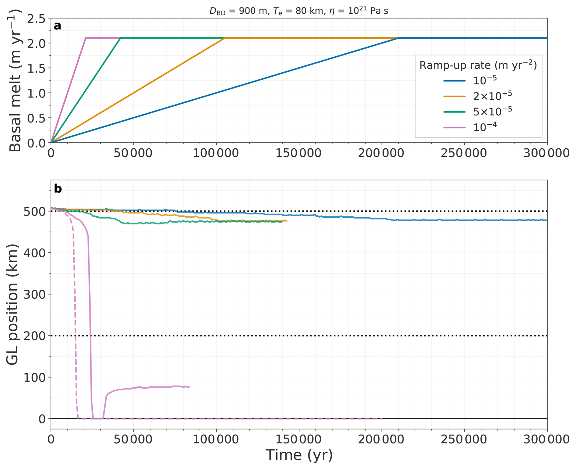
Figure 9 Timeseries of (a) different ramp-up rates of applied sub-ice-shelf melt forcing and (b) associated response of the centerline GL position, highlighting the rate-dependency of a possible ice-sheet destabilization. Dashed line represents the case of a fixed bed. The two dotted horizontal lines mark the range of retrograde bed slope for a fixed bed.

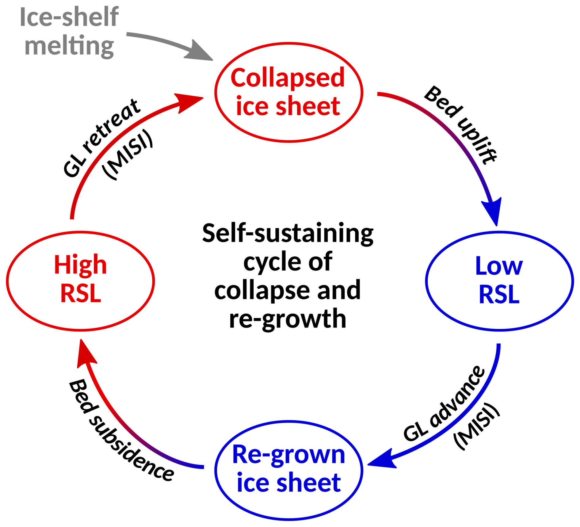
Figure 10 Cycle of processes underlying the self-sustaining oscillations between advanced and collapsed ice-sheet states.

In the event of R-tipping, the decrease in the tipping threshold relative to the B-tipping threshold, Δm_R-tip (Eq. 2), ranges between 7 % and 62 % (Fig. S5). In the case of a shallow initial bed depression, this reduction of the effective tipping threshold for larger forcing rates generally strengthens with increasing η (Fig. S5c), which is in accordance with findings from Swierczek-Jereczek et al. (2026) which are based on numerical experiments that vary Antarctic upper-mantle viscosities but leave the field of the lithosphere thickness fixed in all simulations. Altering the lithosphere thickness in our simulations, in most cases we find a stronger reduction of the effective tipping threshold for decreasing T_e, i.e., a stronger increase of the B-tipping threshold Δm_B-tip compared to the R-tipping threshold Δm_R-tip, leading to larger R-tipping ranges in Figs. 6 and S4. In this regime of stronger basal melting the destabilizing MISI feedback is enhanced through the strong reduction of ice-shelf buttressing and GL retreat into regions of steeper retrograde bed slope, resulting in potentially faster GL retreat timescales that lead to tipping at lower basal meltrates if the rate of meltrate increase is sufficiently fast. The largest absolute values of Δm_R-tip (≈40 to 60 %) are found in the lower-right corner of the parameter space, representing rather unrealistic solid-Earth conditions. More realistic parameter combinations (closer to the diagonal of the parameter space; see Figs. 6 and S4) yield a range of Δm_R-tip from 7 % to 40 %.

Occurrences of R-tipping that we detected for the backward branch of the hysteresis are discarded since in no case the R-tipping range is larger than the sampling rate of 0.1 m yr⁻¹ used to infer B-tipping thresholds. Moreover, comparability within our ensemble would be limited due to the fact that the backward branches of the different model realizations start from different ice-bed geometries and different meltrates (ranging from 3 to 20 m yr⁻¹ as opposed to 0 m yr⁻¹ which is the same initial meltrate value for all runs of the forward branch). The negligible occurrence of backward R-tipping in our simulations can be explained by the fact that prior to the tipping of the ice sheet towards its advanced state almost no bed response takes place (Fig. 4c), i.e., a fundamental requirement for R-tipping is lacking here.

The coupled ice-bed evolution simulated in our experiments shows a clear dependency on the lithosphere thickness, i.e., the B-tipping thresholds increase with decreasing lithosphere thickness, and this increase is particularly strong towards the lower end of the applied T_e range (m_B-tip ranges between 1.3 and 3 m yr⁻¹ for T_e≥80 km but reaches up to 18 m yr⁻¹ for T_e=20 km; see Fig. S5). We attribute this strong dependency to the influence of the lithosphere thickness on the horizontal extent (locality) of the bed response to ice-load changes (e.g., Gomez et al., 2015; Konrad et al., 2015; Coulon et al., 2021). That is, a thinner lithosphere induces a bed response that is less widespread in the horizontal and thus more localized to the GL region (where the largest ice-load change occurs), resulting in larger rates of local bed elevation change. Consequently, thinner lithospheres can strengthen the stabilizing effect of bed uplift in the course of GL retreat and thus increase critical thresholds of collapse. In fact, in simulations by Konrad et al. (2015) the small difference between T_e=40 to 60 km decides whether the long-term evolution of the WAIS ends in a collapsed state or not (see their Fig. 5B).

However, a series of previous studies found that the model response only weakly depends on the prescribed lithosphere thickness (e.g., Whitehouse et al., 2012; Milne et al., 2018; Coulon et al., 2021; Swierczek-Jereczek et al., 2024). We would like to stress that these results do not contradict ours, simply due to the fact that most of these studies differ substantially from the present study. That is, often these studies are characterized by one ore several of the following aspects: First, the simulations either prescribe an ice loading history or introduce an ice body that remains fixed in time, making the ice-bed interaction one-directional. Consequently, the (changing) ice load induces a solid-Earth response but this response does not feed back to the ice-sheet evolution and thus the simulations do not account for the interaction of feedback loops shown in Fig. 1 which is central to the strongly stabilizing effect we see for low T_e values. Second, the applied forcing rates are much higher than the very slow forcing rates that we use here to achieve quasi-equilibrium conditions. This implies a dependency of the results not only on the viscous response timescale of the solid-Earth structure but also on the applied forcing rate. In fact, for the weaker forcing scenarios (lower forcing rates) applied in Coulon et al. (2021) the influence of the lithosphere thickness increases and the influence of the viscosity timescale decreases, which is in accordance with our results. While Swierczek-Jereczek et al. (2026) apply similarly slow forcing rates like the ones used here, their T_e field is the same in all simulations, making it hard to deduce explicit statements on the sensitivity of the results on the lithosphere thickness. Third, the applied T_e values generally lie above the low end of the range of lithosphere thicknesses used here to which our results are most sensitive (the minimal value used in the above mentioned studies is T_e=50 km, except for Coulon et al. (2021) who use a range of 10 to 40 km in West Antarctica). In summary, the quasi-equilibrium simulations carried out here in combination with a wide sampling of the prescribed solid-Earth parameters reveal the potentially strong influence of the lithosphere thickness on the bifurcation point of a MISI-prone outlet glacier that interacts with the underlying solid Earth. In other words, approaching the system's bifurcation point very slowly, as done in this study, demonstrates the strong potential of a very localized and fast bed deformation (due to a weak Earth structure) to add resilience to the system, increasing the critical threshold of collapse (compared to a more widespread response or the case of a fixed bed).

To investigate the sensitivity of our results to the steepness of the retrograde bed section, which plays a major role in the MISI mechanism, all simulations were carried out for a shallow (D_BD=300 m) and a deep initial overdeepening (D_BD=900 m), respectively (Fig. 2). This way, large-scale characteristics of the retrograde bed slopes of different Antarctic regions are reflected in our study. For the shallow overdeepening the initial average magnitude of the retrograde slope of $\mathrm{1}\times {\mathrm{10}}^{-\mathrm{3}}$ (1 m elevation change per km) resembles the more gentle bed slopes of the continental shelves below Antarctica's Ross and Filchner-Ronne ice shelves (Kingslake et al., 2018, see their Extended Data Fig. 3). In the case of the deep overdeepening, the average retrograde bed slope is steeper by a factor of three ($\mathrm{3}\times {\mathrm{10}}^{-\mathrm{3}}$) and is comparable to the observed magnitude of bed drop along a transect through Thwaites Glacier (bed drop of about 750 m over the first 250 km upstream of its GL; Morlighem et al., 2020; Sergienko and Wingham, 2022). While a steeper retrograde bed slope generally implies a lower absolute B-tipping threshold, m_B-tip, in our simulations, relevant differences in B-tipping threshold increase relative to the fixed-bed case, Δm_B-tip, only occur for the thinnest lithosphere applied (Fig. S5a, b). In this case, our model setup of steep (Thwaites-like) retrograde slope yields Δm_B-tip values that are roughly halved compared to our setup of a three times shallower retrograde slope. This suggests that WA-type bed characteristics are particularly effective in delaying or even preventing (self-reinforcing) ice-sheet retreat in regions of shallow retrograde bed slopes. Ranges of R-tipping are generally slightly larger in the case of the shallow retrograde slope (Figs. 6 and S4).

All of the simulations exhibiting R-tipping show a GL overshoot in the aftermath of ice-sheet collapse, i.e., a temporary retreat of the GL beyond its ultimate (further downstream) equilibrium position. The magnitude of the GL overshoot is more pronounced for a (1) higher upper-mantle viscosity due to the larger lag between ice-mass change and bed response, (2) thinner lithosphere due to the more localized bed uplift promoting GL re-advance and (3) shallower pro-grade bed slope of the inland sill that eases both GL retreat and subsequent re-advance. Kingslake et al. (2018) provide paleo evidence for extensive overshoots of West Antarctica's GLs since the Last Glacial Maximum, based on the same physical mechanism: the delayed bed rebound in response to large-scale ice-sheet retreat induces GL re-advance. Kingslake et al. (2018) suggest that these overshoots took place on a scale of several hundred kilometers in Antarctica's Ross and Weddell Sea Sectors, partly facilitated by the uplift of regional ice rises that enhanced ice-shelf buttressing. They modeled such GL overshoots in paleo simulations using PISM with the same LC model as used here, prescribing upper-mantle viscosities of $\mathit{\eta }\ge \mathrm{5}\times {\mathrm{10}}^{\mathrm{20}}\mathrm{Pa}\mathrm{s}$ (lithosphere thickness ranging from T_e=40 to 90 km). In our simulations, GL overshoots occur for a similar range of solid-Earth parameter configurations ($\mathit{\eta }\ge \mathrm{5}\times {\mathrm{10}}^{\mathrm{19}}\mathrm{Pa}\mathrm{s}$ and T_e≤140 km) but the overshoot size is smaller in most instances (ranging from several 10 up to 150 km), numbers which are not only determined by the three conditions mentioned above but also by the length scale of our topographic setup.

Conditions that produce sufficiently large GL overshoots in our simulations lead to self-sustaining oscillations between ice-sheet collapse and re-advance (Figs. 10, S4o, p and Movie S2, Feldmann, 2026d). The oscillations are self-sustaining since – once a critical forcing threshold is crossed – they continue perpetually under constant external forcing solely due to the internal interaction between ice-sheet dynamics and solid-Earth. The oscillations show characteristics of Heinrich events, i.e., periodic phases of abrupt ice discharge of the Laurentide Ice Sheet which are suggested to have occurred during the last glacial period (Heinrich, 1988). The mechanism underlying our simulated oscillations between retreated and re-grown ice-sheet states is internally-driven, similar to the “binge-purge” mechanism described by MacAyeal (1993), and in contrast to several external, climate-forcing driven mechanisms (Hulbe et al., 2004; Alvarez-Solas et al., 2013; Bassis et al., 2017), suggested to explain the periodic occurrence of Heinrich events. While the binge-purge theory is based on thermodynamics at the ice-bed interface (neglected here), the mechanism in our simulations relies on the purely mechanical interaction between ice-sheet dynamics and the deforming solid Earth. A theory proposed by Bassis et al. (2017) also involved the process of bed deformation though not as the direct cause of reversing collapses/advanced ice-sheet states (as in our study) but acting as a control to the external ocean forcing. Simulations by Zeitz et al. (2022) showed large-scale oscillations of Greenland's ice volume resulting from the interaction between ice-sheet dynamics, bed deformation and elevation-dependent surface melting and precipitation. We emphasize that the very simple mechanism of cyclic ice-sheet collapse and re-growth described here should not explain the occurrence of Heinrich events but rather highlight that under certain conditions the basic interaction between ice sheet and solid Earth alone can lead to large-scale, cyclic events of ice-sheet collapse and re-growth that resemble the abrupt characteristics of Heinrich events. Also note that estimates of the solid-Earth structure beneath the Laurentide Ice Sheet (ranges of T_e= 100–180 km and $\mathit{\eta }=\mathrm{0.2}-\mathrm{0.5}\times {\mathrm{10}}^{\mathrm{21}}\mathrm{Pa}\mathrm{s}$, according to Zhao, 2013; Argus et al., 2021) do not correspond to parameter combinations that produce the self-sustained oscillations in our experiments (T_e=20 km and η≥10²¹ Pa s).

The rates of the slow forcing ramp-up/down prescribed in the hysteresis experiments are chosen such that the response of the coupled system is generally in quasi-equilibrium with the forcing. That is, the very slow forcing rate induces a very slow response of the ice discharge (ice-load change) so that the associated solid-Earth response remains close to equilibrium with respect to the ice-load change. However, a perfect equilibrium response would be achieved only for an infinitely slow forcing rate, which is possible only in theory. As a result, the B-tipping thresholds inferred here are likely biased towards lower values as the application of even slower forcing rates would allow for a more complete response of the solid Earth (more uplift) to each increment of GL retreat. This particularly applies to the highest viscosity value prescribed in our ensemble ($\mathit{\eta }=\mathrm{5}\times {\mathrm{10}}^{\mathrm{22}}\mathrm{Pa}\mathrm{s}$), associated with a timescale on the order of 100 000 years, compared to a timescale on the order of 1000 to 10 000 years for the next-lower viscosity value (η=10²¹ Pa s; see Table A1 and Fig. A). For the highest viscosity value we thus reduced the forcing rate by one order of magnitude (forcing rate $\dot{m}={\mathrm{10}}^{-\mathrm{6}}\mathrm{m}{\mathrm{yr}}^{-\mathrm{2}}$ equals a meltrate increase of 0.1 m yr⁻¹ per 100 000 years) compared to the rest of the ensemble ($\dot{m}={\mathrm{10}}^{-\mathrm{5}}\mathrm{m}{\mathrm{yr}}^{-\mathrm{2}}$ equals a meltrate increase of 0.1 m yr⁻¹ per 10 000 years). The very long response timescale of the ensemble members with $\mathit{\eta }=\mathrm{5}\times {\mathrm{10}}^{\mathrm{22}}\mathrm{Pa}\mathrm{s}$ affects the determination of the bifurcation points in another way: a precise estimate of the B-tipping thresholds would ideally require very long branch-off simulations in that case, each covering a time span of more than 1 000 000 model years, an effort we cannot make due to the numerous branch-off simulations and the limited computational capacities. Thus, our branch-off simulations (duration of up to several 100 000 model years) may overestimate the B-tipping thresholds for the ensemble members with $\mathit{\eta }=\mathrm{5}\times {\mathrm{10}}^{\mathrm{22}}\mathrm{Pa}\mathrm{s}$, contrary to the general potential bias towards lower values due to the finite ramp-up rates mentioned above.

Note that for simplicity we use a fixed bed topography during the ice-sheet spinup, such that the subsequent ramp-up experiments start from the same ice-sheet state and the same bed topography (for a given D_BD value). This approach involves the assumption that the ice-sheet geometry is in equilibrium with the same underlying bed geometry, regardless of the specific solid-Earth structure. Naturally, both the ice and bed components would freely evolve into equilibrium in an interactive way, resulting in a specific steady-state geometry of the bed and the ice sheet for each solid-Earth configuration. The centerline profiles resulting from this approach are shown in Figs. S2 and S3 (bed deformation switched on during spinup but otherwise the spinup procedure is the same as described in Sect. 2.2). In this case, the spun-up ice sheets generally have a greater horizontal extent (GL more advanced in main flow direction) which also leads to an overall thicker ice body: while the initial ice block evolves, the deformable bed allows for subsidence where the ice sheet is grounded and uplift on the oceanward side of the coastal sill, where the ice is floating. This pattern is more pronounced for thinner lithospheres due to the more localized response, i.e., a stronger response under and closely around the ice load, resulting in more advanced, thicker ice sheets. The self-sustaining “forebulge feedback” which promotes ice-sheet advance toward the continental shelf edge as seen here (a mechanism that is enhanced for thinner lithospheres) is described in Albrecht et al. (2024) based simulations with PISM coupled to the state-of-the-art 3D VIscoelastic Lithosphere and MAntle model (VILMA). While the alternative spinup method described above has the advantage of delivering a variety of self-consistent equilibrium ice-bed configurations it would substantially limit the comparability of the coupled ice-bed evolution between different model configurations which we strive for in this study.

The LC model applied in this study to model the visco-elastic solid-Earth response accounts for the effect of bed deformation but neglects gravitational and rotational sea-level effects as well as lateral variations in the mantle viscosity and elastic lithosphere thickness. Taking into account the gravitational pull of the ice masses and the associated effect on the regional sea-surface height would likely enhance the stabilizing GIA feedback shown in Fig. 1: ice-mass loss (gain) in the course of ice-sheet retreat (advance) would immediately reduce (increase) the pull on the regional water masses and thus decrease (increase) the relative sea level regionally, hampering GL retreat (advance). The incorporation of this effect would thus likely lead to higher (lower) thresholds of ice-sheet collapse (re-advance) throughout our ensemble of simulations. Rotational effects as a result of mass redistribution on the sphere produce rather far-field sea-level patterns, and can be neglected for the regional processes considered in our experiments (Gomez et al., 2018). In reality, we find a laterally and vertically varying 3D Earth structure, such that the visco-elastic response varies regionally, being locally affected by the efficiency of the viscous material flow through the mantle from or to neighboring regions (e.g., Albrecht et al., 2024; van Calcar et al., 2025). For our experiments with homogeneous low mantle viscosity and hence efficient material transport we evaluate the inferred rate and magnitude of the visco-elastic deformational response as an upper bound.

Despite the limitations of the applied simplified GIA model discussed above, our results account for the leading-order effect of the ice-bed interaction in the course of MISI-driven retreat or advance and allow for a computationally efficient application in ensemble simulations. A comprehensive investigation of combined gravitational, rotational and deformational effects would require the application of a more complex and computationally demanding 3D GIA and sea-level model (e.g., Albrecht et al., 2024) instead of the rather simple and fast 1D LC model used here (see Swierczek-Jereczek et al., 2024, for an overview of commonly used GIA model classes).

Our model setup involves further simplifying assumptions that affect the results: the accumulation rate at the ice surface, the friction coefficient at the ice base and the ice softness (ice temperature) each are chosen to be uniform across the entire model domain and constant in time. Processes like ice fracturing, strain heating or melting of the ice at the surface or the grounded ice base are neglected. While this approach is strongly simplified compared to the complexity of the real world, it allows us to focus on the interaction between ice dynamics and the evolving solid Earth, avoiding potential interference with effects from other processes that would complicate the analysis and dilute the focus of this study. A comprehensive investigation of the tipping dynamics of the Greenland and Antarctic ice sheets and other important tipping elements of the Earth system that accounts for the complex nature of each element and also their potential interaction, using realistic model setups and involving state-of-the-art Earth System Models, is the aim of the Tipping Points Modelling Intercomparison Project (TIPMIP, Winkelmann et al., 2025).

While the friction coefficient entering the Weertman-type friction law used here is prescribed to be spatially and temporally uniform, the basal stresses calculated from the friction law are not as they depend on the basal ice velocities which, in turn, are diagnosed from the non-local SSA stress balance governing the ice flow. Since the basal stresses are integral part of solving the SSA stress balance which also involves the gravitational driving stress and horizontal membrane and shear stresses, the stress fields adjust over time, in particular allowing for the formation of the ice stream inside the bed trough of the setup (Fig. S1).

Taking into account thermo-mechanically coupled flow in our simulations would involve strain heating and generation of meltwater at the ice base due to frictional heating (Feldmann and Levermann, 2017). It has been shown in idealized hysteresis experiments of a flowline ice sheet that thermo-mechanical coupling can result in a substantial widening of the bistability regime (Moreno-Parada et al., 2025): variations in the ice sheet's temperature field allow the ice sheet to adjust to perturbations due to the feedback between evolving ice thickness, viscosity structure, internal stresses and ice flux. Moreover, our simulations do not account for changes in the surface accumulation. According to idealized experiments by Sergienko (2022) the feedback emerging from the generally strong dependency of snowfall and surface melting on the elevation (atmospheric temperature) can substantially affect ice-sheet (in-)stability.

We use a spatially uniform sub-ice-shelf meltrate as the single control parameter to alter ice-shelf buttressing in our hysteresis experiments which is observed to be the main mechanism driving Antarctic ice-sheet retreat over the past decades. Applying a realistic, spatially heterogenous meltrate pattern would likely alter our results. According to observations, basal meltrates are typically strongest close to the GL beneath the thickest portion of the ice shelf (e.g., Dutrieux et al., 2013; Shean et al., 2019; Adusumilli et al., 2020). In some places, observations show concentrated melting at the lateral ice-shelf shear margins (Berger et al., 2017; Shean et al., 2019; Alley et al., 2019) which would accelerate buttressing loss (Feldmann et al., 2022), strengthening the MISI feedback in our simulations and thus lead to lower tipping thresholds.

5 Conclusions

In summary, our results highlight how crucially the type of the solid-Earth structure underlying a MISI-prone ice sheet can affect its tipping dynamics in a qualitative and quantitative way, based on the tightly coupled evolution of ice sheet and bed and the involved (de-)stabilizing feedbacks: weak (West-Antarctic type) solid-Earth structures efficiently counteract MISI initiation due to a very fast and localized bed uplift that fuels a strong stabilizing GIA feedback. Conversely, strong (East-Antarctic type) solid-Earth structures, responding comparatively slow to ice-mass changes, can substantially reduce critical tipping thresholds for a sufficiently fast forcing rate, i.e., lead to the occurrence of R-tipping. Furthermore, a more localized and slower solid-Earth response promotes GL overshoot, which, in case of sufficiently shallow bed slopes, can result in the occurrence of self-sustaining oscillations between advanced and collapsed ice-sheet states, induced solely by the dynamic interaction between ice sheet and solid Earth. Regarding projections of the future stability of the Antarctic Ice Sheet and its associated sea-level contribution, our results in particular suggest that considering both the magnitude and the rate of future anthropogenic greenhouse gas emissions driving global warming as well as a careful spatial and temporal representation of Antarctic bed deformation with associated uncertainties are key for making insightful statements.

Appendix A: Timescales

A1 Maxwell times

Due to the assumption of a linear-viscous Maxwell rheology made in the LC model, the timescale of the viscous response of the solid Earth to ice-load changes, named τ_SE hereafter, scales linearly with the mantle viscosity η. That is, for two different mantle viscosities η and η^′ and the associated timescales τ_SE(η) and τ_SE(η^′), it holds

$$\begin{array}{}\text{(A1)}& {\displaystyle \frac{{\mathit{\tau }}_{\mathrm{SE}}\left(\mathit{\eta }\right)}{{\mathit{\tau }}_{\mathrm{SE}}\left({\mathit{\eta }}^{\prime }\right)}}={\displaystyle \frac{\mathit{\eta }}{{\mathit{\eta }}^{\prime }}},\end{array}$$

giving relative timescales of the solid-Earth response. To infer the absolute timescales, we carried out a small set of additional perturbation experiments, modeling only the viscous response of the bed: starting from the same initial equilibrium that is used in the ensemble simulations, the entire ice load is removed instantaneously, inducing abrupt bed uplift. That is, the isostatic equilibrium between ice sheet and solid Earth (dashed grey centerline profiles in Fig. S2) is perturbed due to the ice-sheet removal and in response the bed lifts up until it converges to a new equilibrium on a viscosity-specific timescale, which we infer by an exponential fit to the curve of bed-elevation change (Fig. A1). For the lowest applied upper-mantle viscosity, η_min=10¹⁸ Pa s, the fit yields τ_SE(η_min)≈9.5 years. Based on this value, the linear scaling according to Eq. (A1) then results in fitted curves that match the simulated curves for each of the higher mantle viscosities to a good approximation (summarized in Table A1). Note that the timescales inferred here should serve as first-order estimates since they are based on simulations with a single lithosphere thickness (T_e=80 km) that use the same ice-sheet length and bed-depression depth. A more accurate estimation of the τ_SE values would involve the variation of T_e and the geometry of ice-sheet and bed.

Table A1 Scaling of response times of the solid Earth, τ_SE, for the upper-mantle viscosities, η, used in the experiments. The second column gives the scaling expected from theory (see Sect. A1), matching with the absolute timescales derived from perturbation experiments (see Fig. A1). For comparison, the absolute response time of the ice load in the absence of bed deformation, is given for the stable regime, τ_L,st, (prior to MISI initiation) as inferred in Sect. A2 and corresponding Fig. A2. We do not have an absolute estimate of the GL response time for the unstable regime, τ_L,MISI, (during MISI). However, the fact that in none of the ensemble simulations bed uplift can stop MISI once it is triggered, suggests ${\mathit{\tau }}_{\mathrm{L},\mathrm{MISI}}<{\mathit{\tau }}_{\mathrm{SE}}$, regardless of the upper-mantle viscosity (fifth column).

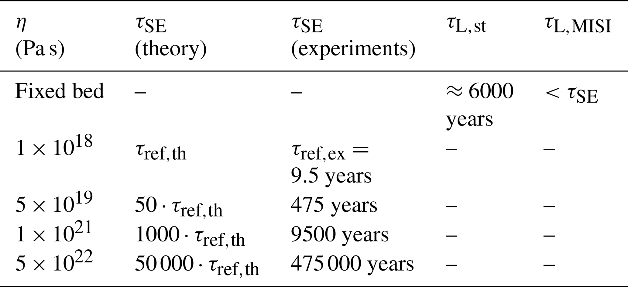
A2 Timescales of GL retreat

Besides the response timescale of the viscous solid-Earth, τ_SE, the other essential timescale in our model configuration is the response time of GL retreat and associated ice-load reduction to a perturbation of basal ice-shelf melting in the absence of bed deformation. For GL retreat in the stable regime, i.e., retreat on the shallow retrograde slope close to the tip of coastal sill, it is on the order of several thousand years (${\mathit{\tau }}_{\mathrm{L},\mathrm{st}}\sim \mathrm{6000}$ years). This value is inferred for the response of the grounded ice load to a basal-melt step forcing from zero to 1 m yr⁻¹ (for D_BD=300 m) and 0.7 m yr⁻¹ (for D_BD=900 m), respectively (Fig. A2). The forcing to values just below the B-tipping thresholds ensures perturbations that are large enough to induce GL retreat while still sufficiently small to avoid triggering a MISI. Similar perturbation experiments that apply an instantaneous step forcing have been carried out in earlier studies (e.g., Pattyn et al., 2013; Feldmann et al., 2014) to investigate and compare the magnitude and timing of ice-sheet GL retreat in simplified setups for different ice-sheet models and grid resolutions.

Note that we do not infer an absolute timescale for unstable GL retreat, i.e., the ice-load change during MISI-driven retreat, τ_L,MISI. Since in all ensemble simulations ice-sheet collapse cannot be stopped by the uplifting bed once a MISI is triggered (even for the lowest upper-mantle viscosity associated with the fastest response time, see Figs. 6 and S4), we deduce that this response time is faster than the viscous response timescale of the solid Earth, τ_SE, regardless of the viscosity value (${\mathit{\tau }}_{\mathrm{L},\mathrm{MISI}}<{\mathit{\tau }}_{\mathrm{SE}}$; see also Table A1).

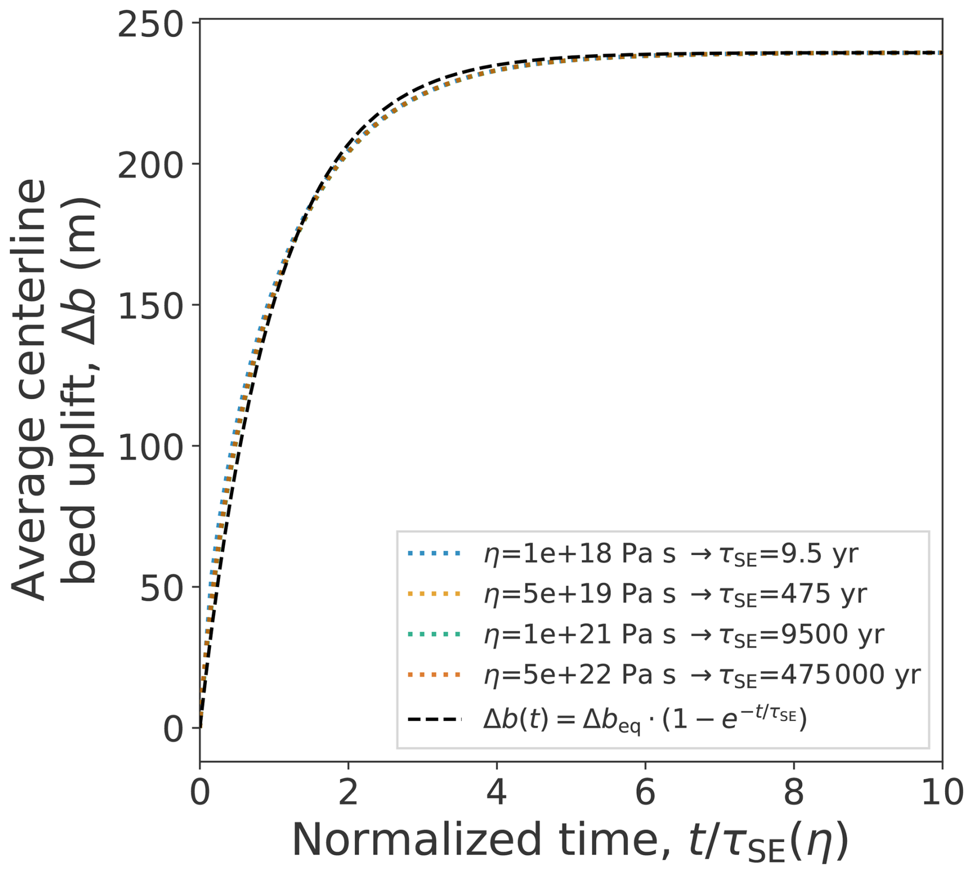
Figure A1 Viscous bed response to an instantaneous removal of the entire ice load for all four upper-mantle viscosities used in this study. Here we choose the bed response, Δb, to be represented by the spatial average of the bed elevation change (uplift) along the centerline of the setup compared to the unperturbed initial steady state. The black dashed line represents the exponential fit according to the function given in the legend with viscosity-specific response timescales τ_SE. Note that for each viscosity value the time axis is normalized to the respective response timescale given in the legend. All curves align and are well approximated by the exponential fit which means that the experimental results obey the theoretically expected timescaling. The final steady-state value of the uplift anomaly is Δb_eq=239 m in all cases. The simulations use a lithosphere thickness of T_e=80 km and an initial bed-depression depth of D_BD=900 m.

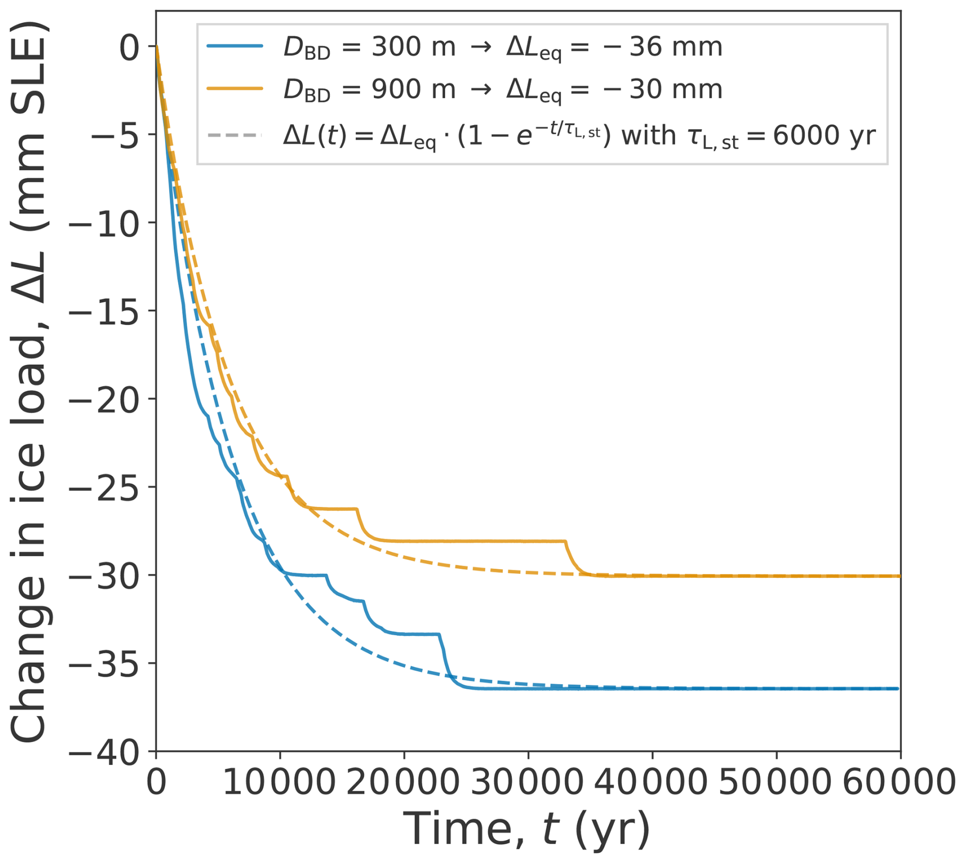
Figure A2 Change in ice load, ΔL, with respect to the initial steady state and associated timescale, τ_L (relaxation time of the ice load), to a basal-melt step forcing of 0.7 m yr⁻¹ that leaves the ice sheet in the stable regime for both bed-depression depths. The dashed lines show the exponential fits according to the equation given in the legend using the respective final steady-state value of ice-load change, ΔL_eq, and a response time of τ_L=6000 years.

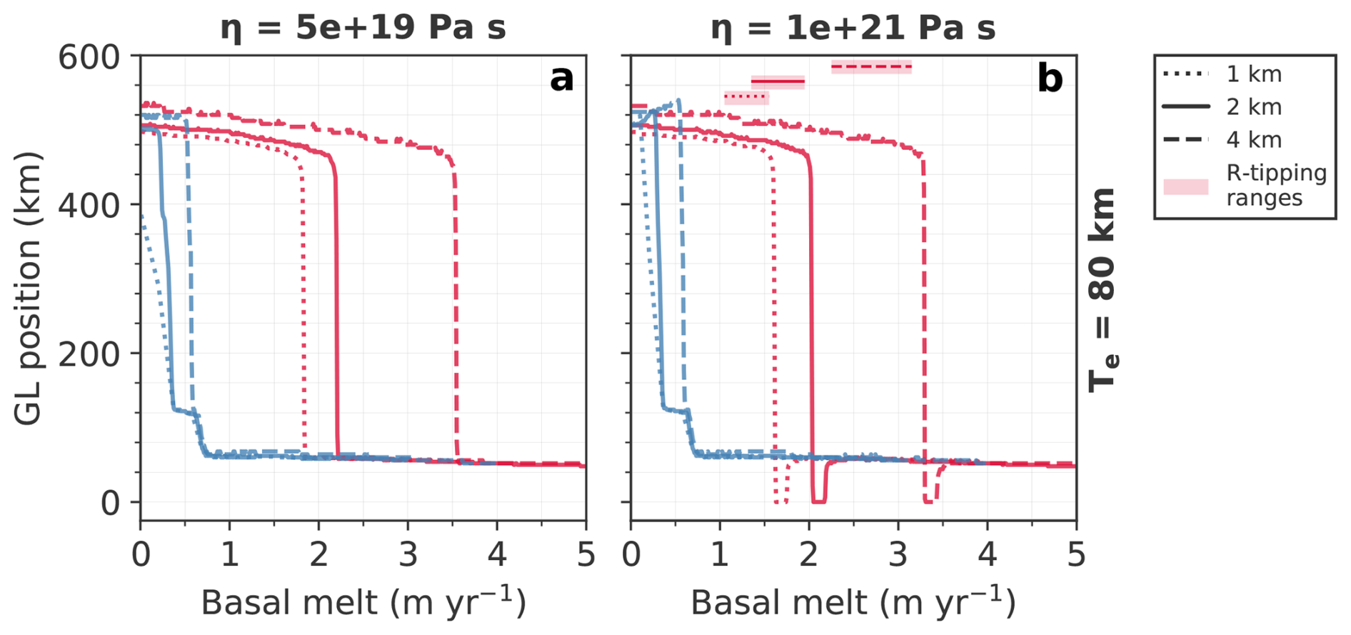
Figure A3 Hysteresis curves for horizontal grid resolutions of 1 km (dotted), 2 km (continuous) and 4 km (dashed) for two representative solid-Earth structures. (a) Parameter pair $(\mathit{\eta },T_{\mathrm{e}})=(\mathrm{5}\times {\mathrm{10}}^{\mathrm{19}}\mathrm{Pa}\mathrm{s},\mathrm{80}\mathrm{km}$), no R-tipping. (b) Parameter pair $(\mathit{\eta },T_{\mathrm{e}})=({\mathrm{10}}^{\mathrm{21}}\mathrm{Pa}\mathrm{s},\mathrm{80}\mathrm{km}$), R-tipping occurs. The R-tipping ranges are show by horizontal red bars with line styles corresponding to the respective resolution.

Appendix B: Grid resolution

To investigate the influence of the grid resolution on our results, we repeated the computation of the hysteresis curves on a finer (1 km) and a coarser (4 km) resolution than the default resolution (2 km) for two representative (η, T_e)-pairs, i.e., (10²¹ Pa s, 80 km) and ($\mathrm{5}\times {\mathrm{10}}^{\mathrm{19}}\mathrm{Pa}\mathrm{s},\mathrm{80}\mathrm{km}$) – the former exhibiting R-tipping, the latter not (Fig. A3). The results show that an increase in the resolution generally leads to a smaller spun-up ice sheet (less advanced GL position), lower B- and R-tipping thresholds for the forward branch of the hysteresis curve and also slightly lower tipping threshold for the backward branch. The results confirm that our choice conducting the ensemble simulations on a 2 km spatial grid is an appropriate compromise between model accuracy and available computational capacities. The results on 2 km resolution are much closer to the results on 1 km resolution than to the results on 4 km resolution. In particular, comparing the two finer resolutions, the R-tipping ranges are shifted but the size of these ranges is very similar. Note that, however, the 2 km resolution is still too coarse to achieve convergence of the results. Unfortunately, we are neither able to run the ensembles of this study on 1 km resolution nor extend the convergence study to even finer resolutions (e.g. 0.5 km), due to the large amount of required computational capacity and time, originating from the combined effect of the very fine spatial grid size and the very slow forcing timeseries.