On the theoretical limitations of joint inversion for basal slipperiness and effective viscosity in ice-flow models

When modelling ice flows there are several aspects which are poorly constrained by observations, in particular parameters related to ice rheology and basal sliding. In computational ice flow models, inversion methods are frequently used to estimate the spatial distribution of these hidden fields. These methods use surface measurement data in combination with a forward model of the ice dynamics that relate the hidden fields to the surface fields. In this study we approximate the forward model using first-order linear perturbation theory to gain insights into our ability to extract information about the ice viscosity at the same time as basal slipperiness, and to understand the theoretical limitations. We frame the inversion problem in terms of a Gaussian maximum a-posteriori estimation with explicitly stated priors for the hidden fields. We illustrate the inversion behaviour with perturbations applied to flow down a laterally confined channel, where both viscosity and slipperiness can play a significant role in the ice sheet dynamics. Our results indicate that it is possible to extract information about the viscosity field at the same time as estimating the basal slipperiness, with strong horizontal gradients in the surface velocity field essential for good viscosity retrieval. We recommend always inverting for basal slipperiness and viscosity together over grounded ice areas in ice-sheet models, and explicitly recognising prior knowledge of the hidden fields in the retrieval through either the inclusion of appropriate priors and regularisation.

1 Introduction

An important component of any modern computational ice-flow model is the initialisation of the model. This ensures that the initial modelled state of the ice sheet, particularly in relation to hidden fields which are poorly constrained by direct observations, creates an ice-flow which behaves in agreement with measurements. The application of inverse methods in the model initialisation to determine the hidden fields dates back to MacAyeal (1992). Since then an increasing number of computational ice-flow models have been developed that include an inversion step in the model initialisation, for example Úa (Gudmundsson, 2025a), BISICLES (Cornford et al., 2015), ISSM (Larour et al., 2012), MALI (Hoffman et al., 2018), STREAMICE (Goldberg and Heimbach, 2013), Elmer/Ice (Gagliardini et al., 2013) and WAVI (Arthern et al., 2015).

This inversion step typically involves minimising the misfit between the modelled velocities (u,v) and observed surface velocities (u_obs,v_obs), with respect to two poorly constrained properties of the ice sheet:

1. The basal slipperiness coefficient, c, which is one of the model parameters entering the sliding law that characterises the basal drag experienced by an ice sheet. Different conventions are used for the definition of this coefficient, but in what follows we always refer to it as basal slipperiness for consistency.

2. The local rheology of the ice characterised by the viscosity, or the rate factor A in Glen's flow law (Glen, 1953) which is the rheological law commonly used in ice-sheet modelling, or some parameterisation of a damage model.

The spatial distribution of one, or both, of these two fields is inferred in the inversion step and then fed into a forward run of the model.

For example, in the Úa ice-sheet model (Gudmundsson, 2025a; Barnes et al., 2021) the misfit between the modelled and observed velocities is defined as

$$\begin{array}{}\text{(1)}& I={\displaystyle \frac{\mathrm{1}}{\mathrm{2}\mathcal{A}}}\int {\left({\displaystyle \frac{u-u_{\mathrm{obs}}}{u_{\mathrm{err}}}}\right)}^{\mathrm{2}}\mathrm{d}\mathcal{A}+{\displaystyle \frac{\mathrm{1}}{\mathrm{2}\mathcal{A}}}\int {\left({\displaystyle \frac{v-v_{\mathrm{obs}}}{v_{\mathrm{err}}}}\right)}^{\mathrm{2}}\mathrm{d}\mathcal{A}\end{array}$$

where $\mathcal{A}=\int \mathrm{d}\mathcal{A}$ is the total area of the domain, and (u_err,v_err) are the data errors in the surface measurements. Note Úa also has the ability to minimise the misfit of the observed surface height change, $\mathrm{d}h/\mathrm{d}t$, measurements in addition to the velocity measurements. Regularisation is often applied to this minimisation procedure. For example, the ice sheet model Úa uses Tikhonov regularisation (Gudmundsson, 2025b; Barnes et al., 2021):

$$\begin{array}{}\text{(2)}& \begin{array}{rl}R& =\sum _{i=\mathrm{1},\mathrm{2}}{\displaystyle \frac{\mathrm{1}}{\mathrm{2}\mathcal{A}}}{\mathit{\gamma }}_{\mathrm{a}}^{\mathrm{2}}\int {\left(p_i-p_{i,\mathrm{prior}}\right)}^{\mathrm{2}}\mathrm{d}\mathcal{A}\\ & +\sum _{i=\mathrm{1},\mathrm{2}}{\displaystyle \frac{\mathrm{1}}{\mathrm{2}\mathcal{A}}}{\mathit{\gamma }}_{\mathrm{s}}^{\mathrm{2}}\int \left|\right|\mathrm{\nabla }(p_i-p_{i,\mathrm{prior}})|{|}^{\mathrm{2}}\mathrm{d}\mathcal{A}\end{array}\end{array}$$

where p_i are each of the hidden fields to be retrieved, and (γ_a,γ_s) are parameters that control the degree of regularisation. The prior estimate for each hidden field, p_i,prior, is often taken as a single starting value set at a realistic scale for the field. The cost function minimised in the step-wise inversion procedure is the sum of the data misfit I and regularisation R terms. Typically the inversion calibrates the velocity misfit to a single snapshot of data, but some recent studies have explored improvements gained from calibrating the model to multiple time snapshots of data (Goldberg et al., 2015; Choi et al., 2023; Surawy-Stepney et al., 2025; Badgeley et al., 2025; Rosier et al., 2025).

While it is common practise to perform this inversion step in the initialisation of ice-sheet models, there are a number of design choices that vary between models; for example the degree of regularisation in the inversion is typically left to the modeller to decide, and yet recent studies on uncertainty quantification have shown that, of the model parameters chosen by the modeller, this is one of the largest contributors to uncertainty in sea level rise projections from Antarctica (Rosier et al., 2025). Even more significant is the choice of whether to perform the inversion jointly for the viscosity and basal slipperiness, or whether to restrict to only solving for basal slipperiness over grounded ice and viscosity over ice shelves, and yet there has been little discussion of this in the literature.

In fact, there is a lack of consensus on whether it is possible to uniquely retrieve the viscosity and basal slipperiness from a joint inversion. For example, simulations with the large-scale ice-sheet models Úa (Gudmundsson, 2025b), WAVI (Arthern et al., 2015) and MALI (Hoffman et al., 2018; Perego et al., 2014), all choose to perform a joint inversion for ice stiffness (a factor related to the viscosity) and basal slipperiness over any model domain that contains grounded ice. The same is true of the ice-sheet model BISICLES (Cornford et al., 2015), although many of the publications using BISICLES stress that regularisation is essential otherwise the joint inversion problem is under-determined, for example Surawy-Stepney et al. (2025) and Trevers et al. (2024). Simulations with the STREAMICE ice flow package of MITgcm (Goldberg and Heimbach, 2013; Goldberg et al., 2015) and the large-scale ice-sheet model ISSM (Larour et al., 2012) choose to restrict to inverting solely for basal slipperiness over grounded ice, believing that extracting information about the viscosity field at the same time is not possible. Similarly, the deep learning ice-flow model IGM (Jouvet et al., 2022) restricts the inversion to a linear combination of the viscosity rate factor and basal slipperiness amid claims that the simultaneous inference of viscosity and basal slipperiness leads to non-unique solutions (Jouvet, 2023). Simulations with the Elmer/Ice ice-flow model (Gagliardini et al., 2013) often only estimate the basal slipperiness through the inversion procedure, for example Jager et al. (2024) and Gillet-Chaulet et al. (2012), although when considering continent-wide ice-sheet simulations a joint inversion with the ice stiffness parameter is often used, for example Caillet et al. (2025).

Despite the disagreement in these modelling approaches, there have been few studies investigating the extent to which ice viscosity and basal slipperiness can be resolved independently when performing a joint inversion procedure. Ranganathan et al. (2021) studied the performance of the joint inversion within the ice-flow model Úa for a synthetic ice-stream, and suggested an improved regularisation scheme weighted by strain rates to improve the accuracy of the estimations. A study by Babaniyi et al. (2021) performed a Bayesian analysis to highlight the large uncertainties that arise from restricting the inversion to only consider the basal slipperiness, and yet these uncertainties are often ignored in practise leading to overconfident and biased results.

The lack of consensus and wide variety of modelling approaches motivates us to investigate the problem from a theoretical stand point, to understand whether it is possible to uniquely retrieve viscosity and basal slipperiness fields through a joint inversion, and what the limitations are with such an approach. Previous work by Gudmundsson and Raymond (2008) developed a theoretical framework using Bayesian inverse methods to understand the limitations of simultaneous retrieval of bed topography and basal slipperiness. The Bayesian inversion maximises the posterior probability of the hidden fields, Φ, given the observed data measurements at the surface, β, to find an estimate for the hidden fields:

$$\begin{array}{}\text{(3)}& \widehat{\mathbf{\Phi }}=\mathrm{argmax}P\left(\mathbf{\Phi }\right|\mathit{\beta })\end{array}$$

The inversion procedure relies on a forward model which relates the hidden properties of the ice-sheet to the observed data measurements at the surface:

$$\begin{array}{}\text{(4)}& \mathit{\beta }=f\left(\mathrm{\Phi }\right)\end{array}$$

The framework developed by Gudmundsson and Raymond (2008) uses a linearised set of equations which relate the perturbations in the hidden fields to perturbations in the surface fields through a set of transfer functions (Gudmundsson, 2003, 2008):

$$\begin{array}{}\text{(5)}& \mathit{\beta }=\mathbf{T}\mathbf{\Phi }\end{array}$$

where the transfer function matrix T has a component for the transference to the surface of each of the hidden fields in Fourier space. These concepts are elaborated on further in later sections. The relationship between the bed characteristics and surface fields has been the subject of study over a number of decades (e.g. Balise and Raymond, 1985; Jóhannesson, 1992; Gudmundsson, 2003). In the analysis by Gudmundsson and Raymond (2008), they derive transfer functions for the bed topography and basal slipperiness, in the context of a uniform slab of ice extending infinitely in all directions and flowing down an inclined place. In this study, we extend their work to include the retrieval of the viscosity field, and derive transfer functions for flow along a laterally confined channel. This more complicated domain, which has horizontal variations in stresses, is an essential part of extending the retrieval to include the ice viscosity.

This paper is organised as follows, in Sect. 2 we describe the forward model which relates the hidden properties of the ice sheet to the surface fields, and present the relevant transfer functions for a laterally confined channel, with the derivation of these transfer functions given in Appendix A; in Sect. 3 we describe the essential points relating to the Gaussian maximum posterior probability inversion procedure, with further details presented in Appendix B. We present our results in Sect. 4. This is split into an analysis within the MAP framework in Sect. 4.1, which assumes a linearisation of the SSA, followed by a numerical inversion within Úa for our synthetic example in Sect. 4.2. We finish with a discussion of the potential impact of the assumptions made in this study in Sect. 5, and a summary of our findings in Sect. 6.

2 The Ice-Flow Forward Model: Transference to the Surface

In this section we describe the linearised forward model used in this study, which relates the hidden properties of the ice sheet to the surface fields, through a set of transfer functions.

We restrict our analysis to ice-flows that can be described by the shallow ice stream approximation (SSA), where the ice thickness is small compared to the horizontal span (MacAyeal, 1989), commonly used in large-scale, vertically-integrated ice-sheet models. The SSA momentum-conservation equations for flow down an inclined plane in a tilted coordinate system aligned to the bed topography are

$$\begin{array}{}\text{(6)}& \begin{array}{rl}& {\partial }_x\left(\mathrm{2}h\mathit{\eta }\left(\mathrm{2}{\partial }_{x}u+{\partial }_{y}v\right)\right)+{\partial }_y\left(h\mathit{\eta }\right({\partial }_{x}v+{\partial }_{y}u\left)\right)-t_{bx}\\ & =\mathit{\rho }gh{\partial }_{x}s\cos \mathit{\alpha }-\mathit{\rho }gh\sin \mathit{\alpha }\\ & {\partial }_y\left(\mathrm{2}h\mathit{\eta }\left(\mathrm{2}{\partial }_{y}v+{\partial }_{x}u\right)\right)+{\partial }_x\left(h\mathit{\eta }\right({\partial }_{x}v+{\partial }_{y}u\left)\right)-t_{by}\\ & =\mathit{\rho }gh{\partial }_{y}s\cos \mathit{\alpha }\end{array}\end{array}$$

where α is the angle of the coordinate system to the horizontal. The driving stresses due to gravity and any pressure gradients are on the right-hand side of the equations. These are balanced on the left-hand side by the basal drag components (t_bx,t_by) and the viscous terms resisting internal deformation (proportional to the vertically-integrated effective viscosity η). In this notation (u,v) are the horizontal velocities in the (x,y) directions respectively; s is the location of the upper glacial surface; h is the ice thickness; and g is the acceleration due to gravity. We use the short-hand ${\partial }_x\equiv \frac{\partial }{\partial x}$.

The viscosity relates the strain rates, ${\dot{\mathit{ϵ}}}_{ij}$, to the deviatoric stresses, τ_ij, in the ice. It is usually modelled by Glen's flow law (Glen, 1953):

$$\begin{array}{}\text{(7)}& {\dot{\mathit{ϵ}}}_{ij}=A{\mathit{\tau }}^{n-\mathrm{1}}{\mathit{\tau }}_{ij}\end{array}$$

Thus $\mathit{\eta }=A^{-\mathrm{1}/n}{\dot{\mathit{ϵ}}}^{(\mathrm{1}-n)/n}/\mathrm{2}$, where A is a temperature-dependent rate factor, and the exponent n varies from n=1 for linear viscous ice to n=4 for dislocation creep. The inversion procedure in numerical ice-flow models either solves directly for the spatial distribution of the rate factor A (Gudmundsson, 2025a, Úa), or they solve for the spatial distribution of an enhancement factor ϕ which represents how far the rate factor deviates from an Arrhenius temperature law (Cornford et al., 2015, BISICLES). The exponent in Glen's flow law is usually set to a fixed value, typically n=3. For the purposes of a standard inversion, which looks at a single point-in-time snapshot of velocity data, spatial variation in n is subsumed into the inferred spatial variation in A. In our study we assume a linear model for viscosity with n=1, so that the viscosity is independent of the strain rates.

The basal drag can be represented by a number of different sliding laws, a common choice being Weertman's sliding law (Weertman, 1957), with basal slipperiness coefficient, c, and sliding exponent, m:

$$\begin{array}{}\text{(8)}& {\mathit{t}}_{\mathbf{b}}=c^{-\mathrm{1}/m}\Vert \mathit{v}{\Vert }^{\mathrm{1}/m-\mathrm{1}}\mathit{v}\end{array}$$

where $\mathit{v}\equiv (u,v)$. Many studies have looked to improve estimates of the appropriate sliding regime for the Antarctic and Greenland ice-sheets using inversion techniques (Hank et al., 2026; Jager et al., 2024). De Rydt et al. (2021) found evidence that the optimal Weertman sliding exponent varied between linear viscous (m=1) to close-to-plastic bed rheology (m≫1) beneath Pine Island Glacier in West Antarctica using surface measurement data at multiple time observations. For the purposes of this study, we follow the standard inversion procedure which estimates the spatial distribution of the basal slipperiness coefficient c, while the exponent in the sliding law is held fixed; a common choice is m=3, although for the purposes of finding analytical solutions in this study we choose m=1.

The constitutive equations in Eq. (6) determine how the viscosity and basal slipperiness impact the surface fields. Notice how the viscosity, η, only ever appears in these equations multiplying the derivatives of the horizontal velocity fields. This means that in the absence of velocity gradients, the viscosity has no visible effect on the surface to first order. This is an important point that should be stressed: horizontal gradients of the velocity field are essential for the viscosity field retrieval in any ice-flow model. This is usually satisfied by ice sheets in the real world.

2.1 Transfer Functions

In this theoretical study, we linearise the SSA equations in Eq. (6) into a set of transfer functions, which relate perturbations in the hidden fields (η and c) to perturbations in the surface velocity fields (u and v) in Fourier space:

$$\begin{array}{}\text{(9)}& \left(\begin{array}{c}\mathrm{\Delta }u\\ \mathrm{\Delta }v\end{array}\right)=\left(\begin{array}{cc}{T}_{u\mathit{\eta }}& T_{uc}\\ T_{v\mathit{\eta }}& T_{vc}\end{array}\right)\left(\begin{array}{c}\mathrm{\Delta }\mathit{\eta }\\ \mathrm{\Delta }c\end{array}\right)\end{array}$$

We derive these transfer functions for our model domain in Appendix A.

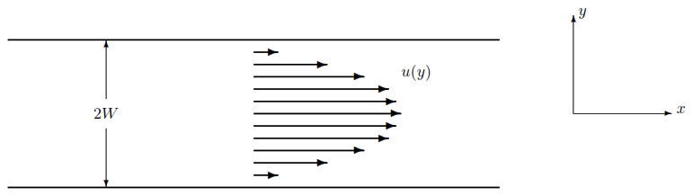
Figure 1 Illustration of the domain geometry. Map plane view of the flow of a slab of ice, of uniform thickness h, down an inclined plane confined in a channel with lateral drag experienced at the side walls. The velocity at the lateral margins is zero.

Previous studies involving transfer functions considered a uniform slab of ice extending infinitely in all directions (Gudmundsson and Raymond, 2008; Gudmundsson, 2008). That scenario has zero spatial gradients in the horizontal velocity fields of the unperturbed state and so, as discussed previously, perturbations in viscosity are not transmitted to the surface. A more realistic scenario, consistent with Antarctic Ice Streams, is flow down an inclined plane laterally confined in a channel; see Fig. 1. In this domain the lateral drag (proportional to viscosity) competes with the basal drag (proportional to slipperiness) to determine the flow characteristics, with the relative contribution influenced by where surface measurements are taken along the flow. The velocity profile has a simple analytical solution for this domain; see Appendix A1 for the derivation:

$$\begin{array}{}\text{(10)}& \stackrel{\mathrm{‾}}{u}\left(y\right)=\stackrel{\mathrm{‾}}{c}{\mathit{\tau }}_{\mathrm{d}}\left(\mathrm{1}-{\displaystyle \frac{\cos h\mathit{\theta }y}{\cos h\mathit{\theta }W}}\right)\end{array}$$

where $\mathit{\theta }\equiv \sqrt{\mathrm{1}/\left(\stackrel{\mathrm{‾}}{c}\stackrel{\mathrm{‾}}{\mathit{\eta }}\stackrel{\mathrm{‾}}{h}\right)}$, and a bar on top indicates the background unperturbed value. The thickness $\stackrel{\mathrm{‾}}{h}$ is constant across the domain and the transverse-to-flow velocity $\stackrel{\mathrm{‾}}{v}$ is zero.

The transfer functions come from considering small amplitude perturbations applied to each of the basal slipperiness and viscosity separately, and deriving the frequency profile of the induced perturbations in the surface measurements; see Eqs. (A6) to (A9) in Appendix A. We consider perturbations in the x-direction for each flowline at a given y along the channel, for which $\stackrel{\mathrm{‾}}{u}\left(y\right)$ is constant, i.e. setting l=0 in the full 2-D transfer functions derived in Appendix A. We focus on the steady-state in these equations, setting t→∞. The normalised transfer functions for the viscosity perturbations are

$$\begin{array}{}\text{(11)}& {\displaystyle }{T}_{u\mathit{\eta }}(k,y)\times {\displaystyle \frac{\stackrel{\mathrm{‾}}{\mathit{\eta }}}{{\stackrel{\mathrm{‾}}{u}}_{\mathrm{0}}}}& {\displaystyle }={\displaystyle \frac{ik{\partial }_{yy}^{\mathrm{2}}\stackrel{\mathrm{‾}}{u}/{\mathit{\theta }}^{\mathrm{2}}\times \stackrel{\mathrm{‾}}{u}/{\stackrel{\mathrm{‾}}{u}}_{\mathrm{0}}}{\mathit{\zeta }}}\text{(12)}& {\displaystyle }{T}_{v\mathit{\eta }}(k,y)\times {\displaystyle \frac{\stackrel{\mathrm{‾}}{\mathit{\eta }}}{{\stackrel{\mathrm{‾}}{u}}_{\mathrm{0}}}}& {\displaystyle }={\displaystyle \frac{-k^{\mathrm{2}}\left({\partial }_{yy}^{\mathrm{2}}\stackrel{\mathrm{‾}}{u}/{\mathit{\theta }}^{\mathrm{2}}+i\mathit{\zeta }/k\right)\times {\partial }_y\stackrel{\mathrm{‾}}{u}/{\stackrel{\mathrm{‾}}{u}}_{\mathrm{0}}}{({\mathit{\theta }}^{\mathrm{2}}+k^{\mathrm{2}})\mathit{\zeta }}}\end{array}$$

and those for the basal slipperiness perturbations are

$$\begin{array}{}\text{(13)}& {\displaystyle }{T}_{uc}(k,y)\times {\displaystyle \frac{\stackrel{\mathrm{‾}}{c}}{{\stackrel{\mathrm{‾}}{u}}_{\mathrm{0}}}}& {\displaystyle }={\displaystyle \frac{ik\stackrel{\mathrm{‾}}{u}\times \stackrel{\mathrm{‾}}{u}/{\stackrel{\mathrm{‾}}{u}}_{\mathrm{0}}}{\mathit{\zeta }}}\text{(14)}& {\displaystyle }{T}_{vc}(k,y)\times {\displaystyle \frac{\stackrel{\mathrm{‾}}{c}}{{\stackrel{\mathrm{‾}}{u}}_{\mathrm{0}}}}& {\displaystyle }={\displaystyle \frac{-k^{\mathrm{2}}\stackrel{\mathrm{‾}}{u}\times {\partial }_y\stackrel{\mathrm{‾}}{u}/{\stackrel{\mathrm{‾}}{u}}_{\mathrm{0}}}{({\mathit{\theta }}^{\mathrm{2}}+k^{\mathrm{2}})\mathit{\zeta }}}\end{array}$$

where we have defined

$$\begin{array}{}\text{(15)}& {\displaystyle }\mathit{\zeta }& {\displaystyle }\equiv \mathrm{2}ik\stackrel{\mathrm{‾}}{u}(\mathrm{1}+\mathrm{2}{k}^{\mathrm{2}}/{\mathit{\theta }}^{\mathrm{2}})-k^{\mathrm{2}}\stackrel{\mathrm{‾}}{h}\stackrel{\mathrm{‾}}{c}{\mathit{\tau }}_{\mathrm{d}}\cot \mathit{\alpha }\text{(16)}& {\displaystyle }{\mathit{\tau }}_{\mathrm{d}}& {\displaystyle }\equiv \mathit{\rho }g\stackrel{\mathrm{‾}}{h}\sin \mathit{\alpha }\end{array}$$

and made use of the relationship, $\stackrel{\mathrm{‾}}{u}=\stackrel{\mathrm{‾}}{c}{\mathit{\tau }}_{\mathrm{d}}+{\partial }_{yy}^{\mathrm{2}}\stackrel{\mathrm{‾}}{u}/{\mathit{\theta }}^{\mathrm{2}}$, for the velocity profile. The transfer functions have been normalised by the basal sliding velocity, ${\stackrel{\mathrm{‾}}{u}}_{\mathrm{0}}=\stackrel{\mathrm{‾}}{c}{\mathit{\tau }}_{\mathrm{d}}$. The transfer functions are a function of the perturbation wavenumber $k\equiv \mathrm{2}\mathit{\pi }/\mathit{\lambda }$, and a function of y, the position of the flow line within the channel. Notice that both viscosity transfer functions drop to zero if the background velocity gradients vanish, and so there will be no induced perturbations at the surface from variations in viscosity to first order.

The transfer functions in Eqs. (11) to (14) are illustrated in Fig. 2. Parameter values were chosen to have similar size contributions from the viscosity and slipperiness transfer functions at an intermediate flow line, $y=\mathrm{40}\stackrel{\mathrm{‾}}{h}$.

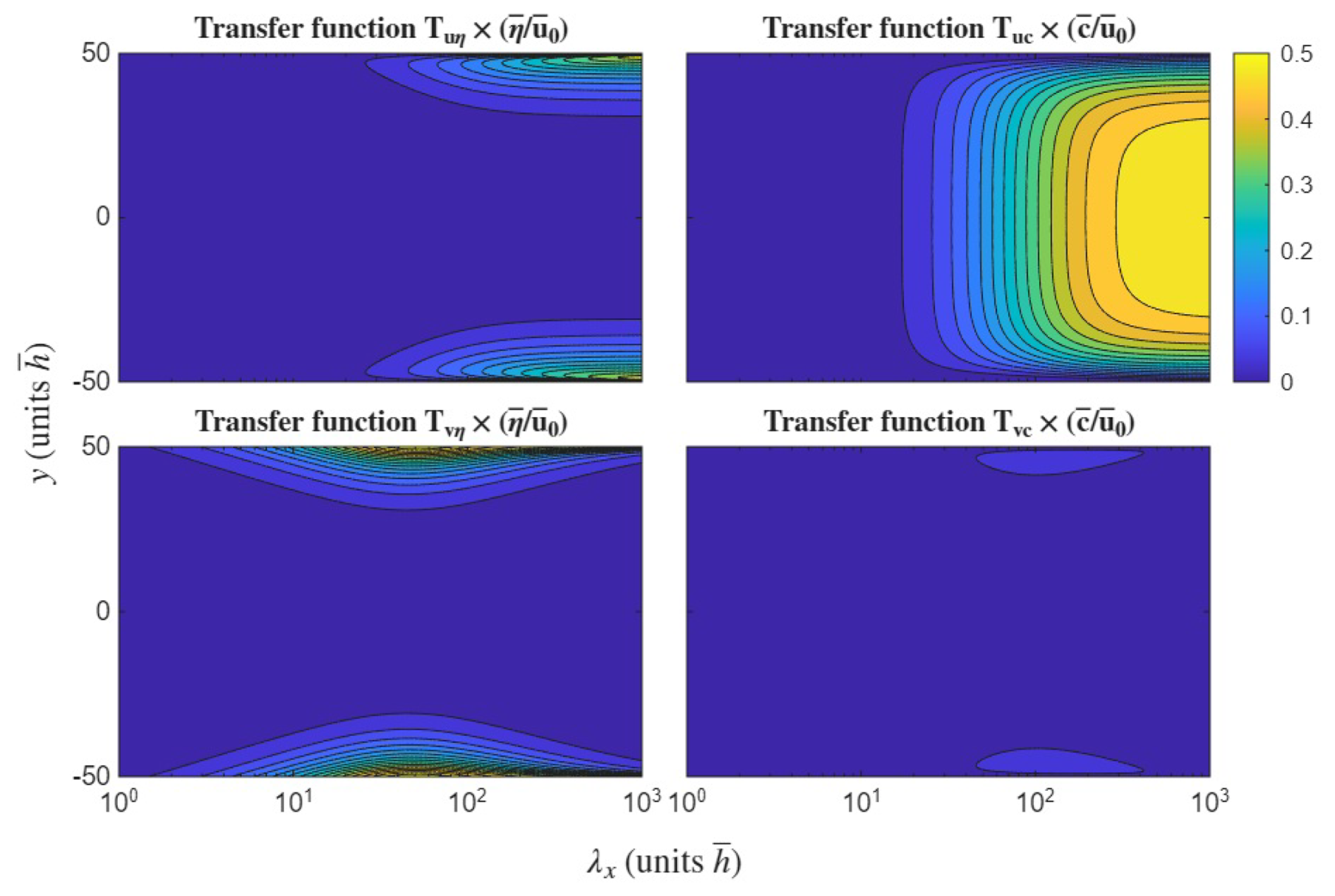
Figure 2 The transfer functions for different flow lines y through the laterally-confined channel, as a function of the perturbation wavelength λ. The viscosity transfer functions, T_uη and T_vη, are on the left; the basal slipperiness transfer functions, T_uc and T_vc, are on the right. The parameters in this example use non-dimensional units: all lengths are normalized by the mean ice thickness; stresses are normalized by the mean basal shear stress; and velocities by mean deformational velocity, such that h=1, τ_d=1, η=0.5. Additionally we have set α=0.05, $W=\mathrm{50}\times \stackrel{\mathrm{‾}}{h}$ and $\stackrel{\mathrm{‾}}{c}=\mathrm{100}$.

At very short wavelengths (k→∞), all the transfer functions tend to zero. These short wavelength perturbations in viscosity and basal slipperiness cannot be retrieved through inverse methods because there are no visible effects on the surface fields. In the long wavelength limit, k→0, the horizontal (along flow) velocity transfer functions tend to

$$\begin{array}{}\text{(17)}& \begin{array}{rl}& \mathrm{|}{T}_{uc}\mathrm{|}\times c/u_c\to \mathrm{0.5}\stackrel{\mathrm{‾}}{u}\left(y\right)/{\stackrel{\mathrm{‾}}{u}}_{\mathrm{0}},\\ & \mathrm{|}{T}_{u\mathit{\eta }}\mathrm{|}\times \stackrel{\mathrm{‾}}{\mathit{\eta }}/{\stackrel{\mathrm{‾}}{u}}_{\mathrm{0}}\to \mathrm{0.5}(\mathrm{1}-\stackrel{\mathrm{‾}}{u}(y)/{\stackrel{\mathrm{‾}}{u}}_{\mathrm{0}})\end{array}\end{array}$$

while the ones transverse to flow tend to zero, where |⋅| denotes the complex modulus of the transfer function. The transference of viscosity perturbations to the surface is maximal at the lateral edges of the domain, where horizontal stresses in the ice are at a maximum, while the slipperiness transfer function is maximal at the centre of the flow where the velocity is greatest.

In the inversion study by Gudmundsson and Raymond (2008), they used transfer functions that had been derived from the full Stokes equations for a uniform slab extending infinitely in all directions (Gudmundsson, 2003). We restrict to the SSA in this study for simplicity, but we expect the impact on the results to be minimal for wavelengths greater than one ice thickness; see Gudmundsson (2008) for a comparison of the Stokes transfer functions to those computed from the SSA.

3 Inversion Procedure

The linearised forward model in Eq. (9), relates the viscosity and basal slipperiness fields to the surface velocity measurements through a set of transfer functions. In principle it can simply be inverted to find the hidden fields for a given set of surface velocity measurements:

$$\begin{array}{}\text{(18)}& \left(\begin{array}{c}c\left(k\right)\\ \mathit{\eta }\left(k\right)\end{array}\right)={\left(\begin{array}{cc}{T}_{uc}\left(k\right)& T_{u\mathit{\eta }}\left(k\right)\\ T_{vc}\left(k\right)& T_{v\mathit{\eta }}\left(k\right)\end{array}\right)}^{-\mathrm{1}}\left(\begin{array}{c}u\left(k\right)\\ v\left(k\right)\end{array}\right)\end{array}$$

In practise, errors in the surface measurements make this an extremely noisy and unreliable estimate. However, it is an important check on the feasibility of the inversion. Inverting this equation is only possible if the transfer matrix T is not singular: det|T|≠0. This is true wherever the transfer functions are non-zero and not linearly dependent. The transfer functions for viscosity are zero in regions of zero velocity gradients (a rare occurrence for ice-streams) and for very short wavelength features. The two sets of transfer functions being linearly dependent is equivalent to saying that there is mixing between the basal slipperiness and viscosity fields, such that the response at the surface is the same for the two fields, as has been suggested in some of the literature (Jouvet, 2023). However, from Eqs. (11) to (14), it is clear that the transfer functions (T_uη,T_vη) are not a linear scaling of the transfer functions (T_uc,T_vc) in general. The two hidden fields have distinct frequency profiles. Thus, in principle, it is possible to extract the spatial distribution of the viscosity field uniquely at the same time as the slipperiness distribution.

To understand how this works in practice with errors in the surface data measurements, we use the theoretical framework developed by Gudmundsson and Raymond (2008), which considers a Bayesian maximum a-posteriori (MAP) estimation with Gaussian probabilities. This also allows us to understand the role of regularisation in the inversion procedure, expressed as a prior distribution in this framework. The minimisation of a cost function, comprising a data misfit and regularisation term as in Eqs. (1) and (2), is equivalent to maximising the a-posteriori distribution in the Bayesian MAP framework with uncorrelated Gaussian measurement errors and a prior distribution modelled using the Matérn covariance function (e.g. Lindgren et al., 2011; Barth et al., 2014). In general, the relationship between the covariance of the prior distribution and regularisation terms in a cost function is not explicit, although it is possible to reproduce a covariance parameterised with Matérn correlation functions using a diffusion operator, as done in FeniCs (Recinos et al., 2023).

We provide details of the MAP estimation framework in Appendix B. We consider retrieval along the x-direction for a particular flowline y=y₀. Prior information about the ice viscosity and basal slipperiness is combined with surface velocity measurements of u(x) and v(x), to give an updated estimate of the viscosity η(x) and basal slipperiness c(x) fields. This estimate maximises the posterior probability according to Bayes' theorem:

$$\begin{array}{}\text{(19)}& P(c,\mathit{\eta }\mathrm{|}u,v)={\displaystyle \frac{P(u,v\mathrm{|}c,\mathit{\eta })P\left(c\right)P\left(\mathit{\eta }\right)}{P(u,v)}}\end{array}$$

The likelihood $P(u,v\mathrm{|}c,\mathit{\eta })$ of the surface measurements, given a particular instance of the viscosity and basal slipperiness fields, is determined by the measurement errors and the forward model. The prior probabilities P(c) and P(η) for the distribution of the viscosity and basal slipperiness fields, respectively, can be chosen to impose smoothness on the retrieved fields.

Measurements and retrieval are at discrete points along the x-direction, which comprise the elements of vectors denoted in bold. The retrieval estimates of the hidden fields are denoted by $\widehat{\mathbf{\Phi }}=(\widehat{\mathit{c}},\widehat{\mathit{\eta }}{)}^{\mathrm{T}}$. As derived in Appendix B, the estimate that maximises the posterior probability is

$$\begin{array}{}\text{(20)}& {\displaystyle }{\widehat{\mathbf{\Phi }}}_{\mathrm{MAP}}{\displaystyle }={\mathbf{C}}_{\mathrm{\Phi }\widehat{\mathrm{\Phi }}}\left({\mathbf{C}}_{\mathrm{\Phi }\stackrel{\mathrm{̃}}{\mathrm{\Phi }}}^{-\mathrm{1}}\stackrel{\mathrm{̃}}{\mathbf{\Phi }}+{\mathbf{T}}_{\mathit{\beta }\mathrm{\Phi }}^{\mathrm{H}}{\mathbf{C}}_{\mathit{\beta }\widehat{\mathit{\beta }}}^{-\mathrm{1}}\widehat{\mathit{\beta }}\right)\end{array}$$

where we have defined

$$\begin{array}{}\text{(21)}& {\displaystyle }{\mathbf{C}}_{\mathrm{\Phi }\widehat{\mathrm{\Phi }}}\equiv {\left({\mathbf{C}}_{\mathrm{\Phi }\stackrel{\mathrm{̃}}{\mathrm{\Phi }}}^{-\mathrm{1}}+{\mathbf{T}}_{\mathit{\beta }\mathrm{\Phi }}^{\mathrm{H}}{\mathbf{C}}_{\mathit{\beta }\widehat{\mathit{\beta }}}^{-\mathrm{1}}{\mathbf{T}}_{\mathit{\beta }\mathrm{\Phi }}\right)}^{-\mathrm{1}}\end{array}$$

which can be thought of as the covariance matrix for the error in the retrieval (Gudmundsson and Raymond, 2008). The data measurements at the surface are denoted by $\widehat{\mathit{\beta }}=(\widehat{\mathit{u}},\widehat{\mathit{v}}{)}^{\mathrm{T}}$, with associated error covariance matrix ${\mathbf{C}}_{\mathit{\beta }\widehat{\mathit{\beta }}}$ which is diagonal for uncorrelated errors. The prior distribution for the hidden fields is assumed to follow a multivariate Gaussian distribution with mean $\stackrel{\mathrm{̃}}{\mathbf{\Phi }}$ and covariance matrix ${\mathbf{C}}_{\mathrm{\Phi }\stackrel{\mathrm{̃}}{\mathrm{\Phi }}}$. The transfer functions in Eqs. (11) to (14) are assumed to perfectly capture the forward model relating the true hidden fields Φ to the true surface fields β in Fourier space, such that

$$\begin{array}{}\text{(22)}& \mathit{\beta }={\mathbf{T}}_{\mathit{\beta }\mathrm{\Phi }}\mathbf{\Phi }.\end{array}$$

where we have defined the combined transfer function matrix

$$\begin{array}{}\text{(23)}& {\mathbf{T}}_{\mathit{\beta }\mathrm{\Phi }}=\left(\begin{array}{cc}{\mathbf{T}}_{uc}& {\mathbf{T}}_{u\mathit{\eta }}\\ {\mathbf{T}}_{vc}& {\mathbf{T}}_{v\mathit{\eta }}\end{array}\right)\end{array}$$

and each transfer function ${\mathbf{T}}_{\star \star }$ is a d×d diagonal matrix, representing the d discrete measurement sites along the flowline, with the transference at each frequency along the diagonal. Note that all the matrices and vectors in these equations have been converted to Fourier space. We can think of the maximum a-posteriori estimate in Eq. (20) as having one component coming from the priors $\stackrel{\mathrm{̃}}{\mathbf{\Phi }}$, scaled by the errors in that estimate, and another component which is an update to the prior estimate coming from the observed surface measurements $\widehat{\mathit{\beta }}$, scaled by their measurement errors.

The mean value of the prior is not significant, it quickly gets updated with the data measurements, but the prior covariance matrix ${\mathbf{C}}_{\mathrm{\Phi }\stackrel{\mathrm{̃}}{\mathrm{\Phi }}}$ is important. It can, for example, determine the relative contribution of different frequencies in the update, or impose a correlation structure on the learnt distribution. In the results that follow, we set the prior mean to zero and choose a covariance matrix which is equivalent to the Tikhonov regularisation in Eq. (2), used in many ice sheet models:

$$\begin{array}{}\text{(24)}& {\mathbf{C}}_{\mathit{\eta }\stackrel{\mathrm{̃}}{\mathit{\eta }}}^{-\mathrm{1}}={\mathit{\gamma }}_{\mathrm{a}}^{\mathrm{2}}\mathbf{I}+{\mathit{\gamma }}_{\mathrm{s}}^{\mathrm{2}}\mathbf{D}\end{array}$$

in Fourier space, where D=diag(k²). The derivation of this covariance matrix is given in Appendix B3. The first regularisation parameter, γ_a, controls the degree to which large amplitude perturbations are suppressed in the retrieval, while the second regularisation parameter, γ_s, controls the suppression of higher frequency perturbations. This form of the covariance matrix effectively assigns higher confidence to the prior for larger k. The end result is a smoothing of the retrieved field. This is particularly important for the retrieval of the basal slipperiness and viscosity where higher frequency perturbations are poorly transmitted to the surface fields. Note, when the variations in the hidden fields are defined as fractional perturbations, then γ_a is dimensionless and γ_s has dimensions of length. We choose the same form for the slipperiness covariance matrix, ${\mathbf{C}}_{c\stackrel{\mathrm{̃}}{c}}^{-\mathrm{1}}$, and construct a block diagonal covariance matrix for the combined covariance matrix, ${\mathbf{C}}_{\mathrm{\Phi }\stackrel{\mathrm{̃}}{\mathrm{\Phi }}}^{-\mathrm{1}}$.

4 Results

4.1 Inversion Procedure within the MAP framework

Here we present the results of the Bayesian maximum a-posteriori inversion applied to our synthetic example of flow down a laterally-confined channel. A sinusoidal perturbation is applied to each of the true viscosity and slipperiness fields, out-of-phase to each other. The resulting perturbations in the true surface fields were derived from the transfer functions. Spatially uncorrelated and normally distributed data errors were added to create the surface velocity measurements. Figure 3 illustrates the retrievals for two different flow lines: one close to the centre of the channel at y=0.2W where the slipperiness field has better transference to the surface; and the other close to the lateral margin at y=0.8W where the velocity gradients are greater and so the viscosity field has better transference to the surface. In these examples we use the same parameter values for the domain as were chosen for the plots of the transfer functions in Fig. 2.

In Fig. 3.a, we see that with almost perfect data (errors of 10⁻⁴ %), the viscosity and basal slipperiness fields can be perfectly retrieved, regardless of the position along the flow. This requires background gradients in the velocity fields, as we have for this synthetic example, otherwise the viscosity field cannot be recovered. The difficulty in the retrieval starts once we add meaningful data errors to the surface velocity measurements. Even for very small data errors (0.005 %) in Fig. 3.b, the retrieval of the viscosity field near the centre of the flow is poor, with significant high-frequency noise in the retrieval. This behaviour is expected from the transfer functions in Fig. 2, which show the poor transference to the surface of viscosity perturbations at the centre of the flow, particularly at smaller wavelengths, and so the surface measurements do not constrain these spurious fluctuations from appearing in the retrieval. The application of a prior (or equivalently regularisation) in Fig. 3c improves the retrieval significantly. The form of the prior covariance matrix in Eq. (24) suppresses the high frequency components in the retrieval. If we increase the magnitude of the surface data measurement errors further to 1 % in Fig. 3d, which is more realistic for current observational accuracy, then regularisation is essential for the retrieval of the basal slipperiness and viscosity anywhere along the flow. With regularisation, the slipperiness is reasonably well retrieved all along the flow (blue and turquoise lines), while the viscosity retrieval struggles even at the lateral margins (red dashed line). The frequency profile of the transfer function will determine how well the regularisation term that scales with k² in the prior covariance matrix suppresses high frequency noise in the retrieval, while at the same time allowing the true perturbation to be recovered. In the case of the viscosity retrieval near the centre of the flow (orange line), this trade off is impossible to satisfy, and the underlying signal cannot be extracted from the noise.

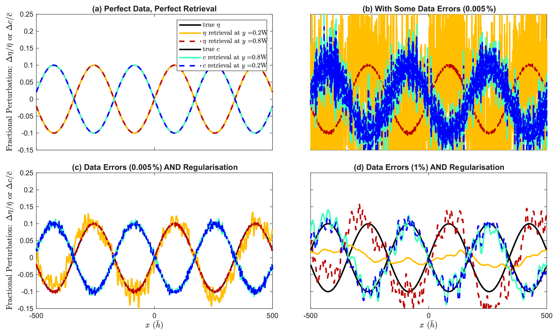
Figure 3 Examples of the retrievals using the MAP inversion along two flow lines for the laterally-confined channel: one towards the edge of the lateral margin at y=0.8W for viscosity η (red) and slipperiness c (turquoise); and one towards the centre of the flow at y=0.2W for viscosity η (orange) and slipperiness c (dark blue). These examples (a) to (d) are for a range of errors in the measurement data, and regularisation parameters of either zero or (γ_a=1, ${\mathit{\gamma }}_{\mathrm{s}}={\mathrm{10}}^{\mathrm{3}}\stackrel{\mathrm{‾}}{h}$). The parameter values for the domain are the same as the example in Fig. 2.

In both Fig. 3c and d, the regularisation parameters used were ${\mathit{\gamma }}_{\mathrm{a}}^{\mathit{\eta }}={\mathit{\gamma }}_{\mathrm{a}}^c=\mathrm{1}$ and ${\mathit{\gamma }}_{\mathrm{s}}^{\mathit{\eta }}={\mathit{\gamma }}_{\mathrm{s}}^c={\mathrm{10}}^{\mathrm{3}}\stackrel{\mathrm{‾}}{h}$, which smoothed the fields without over-constraining towards the prior.

Importantly, there is no evidence of mixing between the viscosity and slipperiness fields. In regions of small background strain rates, the surface data does not provide much additional information about the ice viscosity beyond that provided by the prior, however, this does not translate into less accurate estimates of basal slipperiness in those regions.

4.2 Numerical Inversion in the Laterally Confined Channel

We next consider how this compares to a full numerical inversion within the computational ice-flow model Úa for the same synthetic example of flow down a laterally confined channel. By construction, the analytical results of Sect. 4.1 assumed a linearisation of the SSA forward model using the transfer functions in Sect. 2.1, while the numerical inversion presented here with Úa takes into account non-linear finite-amplitude effects.

As before, a sinusoidal perturbation is applied to each of the baseline viscosity and slipperiness fields along the flow, i.e. feature ridges aligned transverse to flow. The surface data measurements are generated from a forward run within Úa using the prescribed viscosity and basal slipperiness fields, with independent and identically distributed (i.i.d.) Gaussian random noise added to the data points. In Úa the viscosity field is represented by the rate factor A in Glen's flow law, which in the case here of n=1 is equivalent to $A=\mathrm{1}/\mathrm{2}\mathit{\eta }$. We have chosen to invert for the fields in log-space (log A and log c), which is the typical inversion approach in Úa for numerical Antarctic ice flow studies, although the sinusoidal perturbations are applied to η and c, making it identical to the configuration in Fig. 3.

The numerical inversion procedure consists of minimising a functional of the form $J=I+R$, where I and R are given by Eqs. (1) and (2), respectively. The gradients of the function J with respect to A and c are calculated using the adjoint method, and the Hessian obtained using the direct-adjoint method. This approach to calculating the Hessian improves the performance of the minimisation algorithm significantly compared to the commonly-used approximation of the Hessian using the BFGS method. We refer the reader to the Úa Compendium – a technical manual for the Úa ice flow model distributed as part of the software – for further implementation details (Gudmundsson, 2025b).

The inferred viscosity and basal slipperiness fields from this numerical inversion are shown in Figs. 4 and 5, respectively. These inversions have the same configuration as the analytical MAP retrieval in Fig. 3. On the left of each figure is the true A or c field; the top row shows the retrieved field in the case of perfect data; the middle row shows the retrieved fields with realistic noise and no regularisation applied; while the bottom row shows the improved retrieval using regularisation parameters γ_a=1 and γ_s=10³ km (equivalent to the degree of regularisation applied in Fig. 3d).

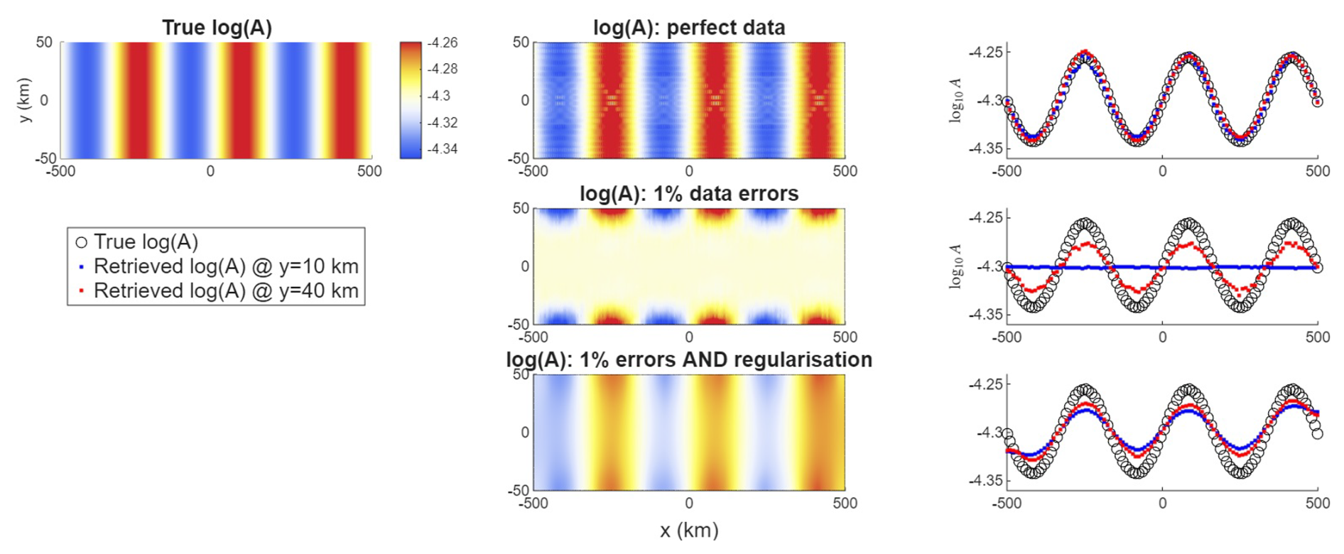
Figure 4 Examples of the viscosity retrieval in Úa for the laterally-confined channel, for a range of data errors and regularisation parameters of either zero or (γ_a=1, ${\mathit{\gamma }}_{\mathrm{s}}={\mathrm{10}}^{\mathrm{3}}\stackrel{\mathrm{‾}}{h}$). We show contour plots of the retrieved field in the two-dimensional domain, and also cut-throughs at y=0.2W and y=0.8W. The parameter values for the domain are equivalent to the example in Fig. 2, but we now use dimensions $\stackrel{\mathrm{‾}}{h}=\mathrm{1000}$ m, τ_d=450 kPa and η=10⁴ kPa yr.

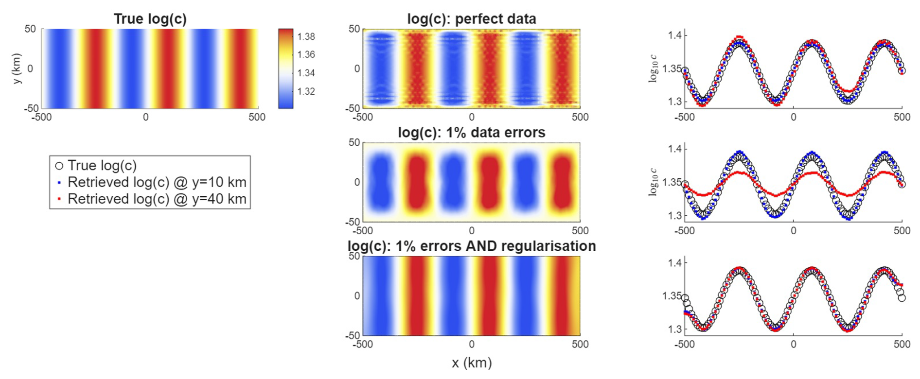
Figure 5 Examples of the basal slipperiness retrieval in Úa for the same experiment as in Fig. 4. for the laterally-confined channel, for a range of data errors and regularisation parameters of either zero or (γ_a=1, ${\mathit{\gamma }}_{\mathrm{s}}={\mathrm{10}}^{\mathrm{3}}\stackrel{\mathrm{‾}}{h}$). We show contour plots of the retrieved field in the two-dimensional domain, and also cut-throughs at y=0.2W and y=0.8W.

One of the first things to note is that with perfect data we get near perfect retrieval of the two fields. This is the same result as we saw in Fig. 3.a and demonstrates, yet again, that viscosity and basal slipperiness can (in principle) be recovered in a joint inversion without unwanted mixing effects. The numerical inversion does introduce some artefacts which are a consequence of the simulation on a finite grid. Introducing some noise to the data measurements, we observe the same pattern of behaviour as seen in the analytical results of Fig. 3. The viscosity retrieval is improved towards the lateral margins where the velocity gradients are larger, while the slipperiness retrieval is best towards the centre of the flow, and there is no evidence of mixing between the viscosity and slipperiness fields.

One of the noticeable differences is that in regions of poor transference to the surface, the analytical MAP inversion had significant high-frequency noise in the retrieval, whereas the numerical inversion with Úa stays close to the initial field values and does not update the estimated A or c.

We find that with regularisation applied, the numerical inversion is even more successful at recovering the hidden fields. This may partly be due to the step-wise nature of the iteration which gradually updates the fields from their initial values; and partly due to considering a two-dimensional grid with regularisation applied along both the x and y directions, rather than the one-dimensional flow line in the analytical example.

These numerical results using Úa reaffirm our findings that it is possible to uniquely retrieve the viscosity and basal slipperiness fields at the same time in an inversion procedure. This adds confidence to our earlier analysis, and provides reassurance that it applies equally to the numerical inversions used in large-scale ice-sheet models. The quality of the retrieval will depend on the magnitude of the data errors and the strength of the horizontal velocity gradients. Regularisation is essential to suppress high-frequency noise components in the retrieval, caused by the poor transference to the surface of perturbations at higher frequencies.

5 Limitations

The results presented in this paper have made a number of necessary simplifying assumptions, so that the inversion procedure could be broken down and understood from a theoretical stand point. In this section we discuss these assumptions and their potential impact.

All experiments have been done with respect to idealised flow down a uniform, laterally-confined channel. Different regions of the flow experience stresses from bed sliding and lateral drag, each to a varying degree, and while the overall flow is simplified, these different regions should be representative of the stresses found within localised regions of a real ice-sheets. The transfer functions derived in this study have distinct frequency profiles, indicating that in general there is not mixing between the viscosity and slipperiness fields. Our expectation is that more complicated stress patterns observed in real ice-sheets should differentiate the transference to the surface of perturbations in slipperiness and viscosity even further.

We have also simplified the flow by assuming linear bed sliding and rheology, when in practice non-linear flow is supported by observations. Higher values of m in the bed sliding law will generally lead to faster velocities, and this will be the dominant impact on the transference to the surface of perturbations in slipperiness. Higher values of n will concentrate higher strain rates into a narrow band close to the lateral margin, and so the gradients in velocity – which are necessary for the transference of viscosity perturbations to the surface – will occur in a narrower region of the domain. Our expectation is that, if anything, values of n>1 and m>1 will likely differentiate the transference to the surface of perturbations in the slipperiness and viscosity even further. Studies by Raymond and Gudmundsson (2005) performed a numerical analysis of the transfer functions for higher order n and m, although applied to the full Stokes equations and with a different background state, which showed limited impact on the amplitude and phase of the transfer functions. Nonetheless, an exploration of the effect of non-linear bed friction and rheology on the inversion could be the subject of a further numerical study exploring the wider parameter space.

Another key assumption feeding into these experiments is that the SSA equations are a true representation of the ice-sheet physics. This approximation is appropriate for shallow ice-sheets where the thickness is small compared to the horizontal span, but will break down for thicker tributaries. In this study we have only considered measurement errors in the surface velocities, and assumed perfect knowledge of the surface elevation, while considering only uncorrelated measurement errors. Relaxing these assumptions could lead to more difficulty in separating the effects of slipperiness and viscosity in the inversion.

Finally, we would like to refer the reader to the transfer functions in Fig. 2. These illustrate the strength of transference to the surface across a range of perturbation frequencies, while the experiments in Figs. 3 to 5 are for a particular choice of perturbation frequency, and for a particular phase shift between the viscosity and slipperiness perturbations. The space of different frequencies and different phase differences for the perturbations hasn't been explored in the experimental results.

6 Conclusions

In this study, we have shown that it is feasible to perform a joint inversion procedure to infer the viscosity and basal slipperiness distribution in ice-sheet models. This does not lead to an underdetermined problem where it is impossible to find a unique solution for the two fields, although our formulation does assume independent measurements of the two horizontal velocity fields (u,v) whereas, for example, BISICLES (Cornford et al., 2015) only considers the magnitude of the velocity.

In this paper, we have explored the inversion procedure from an analytical standpoint. Using a linearisation of the SSA equations, we can visualise the transference to the surface of features in the viscosity and basal slipperiness fields under different conditions. This analytical approach helps us to understand the circumstances where the retrieval is more difficult. For example, the ability to retrieve the viscosity field accurately is strongly dependent on the horizontal stresses within the ice-sheet. Close to the margins of an ice-sheet where lateral drag is causing a significant variation in the horizontal velocity field, the viscosity is well resolved; while closer to the centre of a wide ice-sheet where the flow is uniform, the viscosity is poorly resolved. Short wavelength features in both fields are also difficult to resolve. However difficulty retrieving the viscosity field does not necessarily mean the slipperiness field is more difficult to infer.

Poor retrieval can be assisted by the inclusion of a Bayesian prior for the hidden fields. The inclusion of a prior distribution, for certain forms of the covariance matrix, is equivalent to the regularisation employed in the misfit minimisation in many inversion procedures. Strong confidence in the prior distribution is similar to large regularisation coefficients. Some form of regularisation applied to the two fields is essential as the noise in the surface measurement data increases. This suppresses high-frequency noise in the retrieval and helps the inversion procedure extract the signal within the noise. A strong prior is also necessary for regions where features in the the viscosity are poorly transferred to the surface. Ice-sheet models which ignore spatial variation in the viscosity, during the inversion procedure, are effectively prescribing a prior on the viscosity field with 100 % confidence. We recommend making this choice explicit in the modelling by including the viscosity field as an unknown field in the inversion procedure with strong confidence in the prior, or equivalently large regularisation parameters.

Appendix A: Derivation of the Transfer Functions

In this section we present the derivation of the transfer functions given in Eqs. (11) to (14). These describe the first-order response to small perturbations in each of the two inversion products, viscosity η and basal slipperiness c, separately. We follow closely the technique presented in Gudmundsson (2008) and Schelpe and Gudmundsson (2023), and derive transfer functions for the transient frequency profile of induced perturbations in the surface $h(x,y,t)$, horizontal along-flow velocity $u(x,y,t)$ and transverse-to-flow velocity $v(x,y,t)$. The transfer functions are functions of k and l, the two variables that specify the perturbation wavelength in the along-flow and transverse-to-flow direction, respectively. We consider a reference solution with spatially variable $\stackrel{\mathrm{‾}}{u}$ so that the viscosity contribution doesn't vanish to first-order.

A1 Reference Solution of a Uniform Slab with Lateral Drag

The SSA momentum-conservation equations were given in Eq. (6) and repeated again here for convenience, together with the mass-conservation equation which describes the flow in two-dimensions:

$$\begin{array}{}\text{(A1)}& \begin{array}{rl}& {\partial }_x\left(\mathrm{4}h\mathit{\eta }{\partial }_{x}u+\mathrm{2}h\mathit{\eta }{\partial }_{y}v\right)+{\partial }_y\left(h\mathit{\eta }\right({\partial }_{x}v+{\partial }_{y}u\left)\right)-t_{bx}\\ & =\mathit{\rho }gh\left({\partial }_{x}s\cos \mathit{\alpha }-\sin \mathit{\alpha }\right)\\ & {\partial }_y\left(\mathrm{4}h\mathit{\eta }{\partial }_{y}v+\mathrm{2}h\mathit{\eta }{\partial }_{x}u\right)+{\partial }_x\left(h\mathit{\eta }\right({\partial }_{x}v+{\partial }_{y}u\left)\right)-t_{by}\\ & =\mathit{\rho }gh{\partial }_{y}s\cos \mathit{\alpha }\\ & {\partial }_{x}u+{\partial }_{y}v+{\partial }_{z}w=\mathrm{0}\end{array}\end{array}$$

We consider as a reference solution a grounded ice slab of uniform thickness, extending infinitely in the x-direction, but confined within a channel in the y-direction which exerts lateral drag at the sides. Thus the x-derivatives are set to zero to find the equations describing the background velocity fields (denoted by a bar on top):

$$\begin{array}{ll}{\displaystyle }\stackrel{\mathrm{‾}}{h}\stackrel{\mathrm{‾}}{\mathit{\eta }}{\partial }_{yy}^{\mathrm{2}}\stackrel{\mathrm{‾}}{u}-{\stackrel{\mathrm{‾}}{c}}^{-\mathrm{1}}\stackrel{\mathrm{‾}}{u}& {\displaystyle }=-\mathit{\rho }g\stackrel{\mathrm{‾}}{h}\sin \mathit{\alpha }\\ {\displaystyle }\mathrm{4}\stackrel{\mathrm{‾}}{h}\stackrel{\mathrm{‾}}{\mathit{\eta }}{\partial }_{yy}^{\mathrm{2}}\stackrel{\mathrm{‾}}{v}-{\stackrel{\mathrm{‾}}{c}}^{-\mathrm{1}}\stackrel{\mathrm{‾}}{v}& {\displaystyle }=\mathrm{0}\\ {\displaystyle }{\partial }_y\stackrel{\mathrm{‾}}{v}+{\partial }_z\stackrel{\mathrm{‾}}{w}& {\displaystyle }=\mathrm{0}\end{array}$$

where we have restricted to a Weertman-style sliding law with m=1, such that ${\mathit{t}}_b=c^{-\mathrm{1}}(u,v)$ and these differential equations can be solved analytically. This second-order ordinary differential equation with constant coefficients has a simple well-known solution:

$$\stackrel{\mathrm{‾}}{u}\left(y\right)=A\cosh \mathit{\theta }y+B\sinh \mathit{\theta }y+\stackrel{\mathrm{‾}}{c}{\mathit{\tau }}_{\mathrm{d}}$$

where we have defined

$$\begin{array}{ll}{\displaystyle }{\mathit{\tau }}_{\mathrm{d}}& {\displaystyle }\equiv \mathit{\rho }g\stackrel{\mathrm{‾}}{h}\sin \mathit{\alpha }\\ {\displaystyle }\mathit{\theta }& {\displaystyle }\equiv \sqrt{\mathrm{1}/\left(\stackrel{\mathrm{‾}}{c}\stackrel{\mathrm{‾}}{\mathit{\eta }}\stackrel{\mathrm{‾}}{h}\right)}\end{array}$$

and (A,B) are integration constants. Note the third term on the right hand side is the constant velocity expected from basal sliding without any lateral drag. Applying the boundary condition ${\partial }_{y}u=\mathrm{0}$ at y=0 (due to the symmetry in the problem, the stresses at the centre of the flow must be zero), we find B=0. Additionally, setting the velocity field to zero at the lateral margins, $y=\pm W$, we find $A=-\stackrel{\mathrm{‾}}{c}{\mathit{\tau }}_{\mathrm{d}}/\cosh \mathit{\theta }W$ and $\stackrel{\mathrm{‾}}{v}=\mathrm{0}$. Thus,

$$\stackrel{\mathrm{‾}}{u}\left(y\right)=\stackrel{\mathrm{‾}}{c}{\mathit{\tau }}_{\mathrm{d}}\left(\mathrm{1}-{\displaystyle \frac{\cosh \mathit{\theta }y}{\cosh \mathit{\theta }W}}\right)$$

A2 Viscosity Perturbations

We start by applying a small perturbation to the viscosity of the ice sheet about a constant reference value:

$$\mathit{\eta }(x,y,t)=\stackrel{\mathrm{‾}}{\mathit{\eta }}+\mathcal{H}\left(t\right)\mathrm{\Delta }\mathit{\eta }(x,y)$$

while holding other parameters, such as the basal slipperiness c, constant. We assume the applied perturbation is a step function ℋ(t) with zero perturbation before t=0, and a fixed contribution Δη(x,y) thereafter. This induces small perturbations in the other variables:

$$\begin{array}{}\text{(A2)}& \begin{array}{rl}& h(x,y,t)=\stackrel{\mathrm{‾}}{h}+\mathrm{\Delta }h(x,y,t)\\ & u(x,y,t)=\stackrel{\mathrm{‾}}{u}\left(y\right)+\mathrm{\Delta }u(x,y,t)\\ & v(x,y,t)=\mathrm{\Delta }v(x,y,t)\\ & w(x,y,z,t)=\stackrel{\mathrm{‾}}{w}(x,y,z)+\mathrm{\Delta }w(x,y,z,t)\end{array}\end{array}$$

The reference values, such as $\stackrel{\mathrm{‾}}{u}\left(y\right)$, are those of the steady state solution derived in Sect. A1. The lower surface remains unperturbed, such that $\stackrel{\mathrm{‾}}{h}=\stackrel{\mathrm{‾}}{s}-\stackrel{\mathrm{‾}}{b}$, Δs=Δh, and we assume the lower surface is not spatially varying, i.e. ${\partial }_x\stackrel{\mathrm{‾}}{b}=\mathrm{0}$.

Substituting the expressions in Eq. (A2) into the equations of motion (A1) and keeping terms to first-order in the perturbations, we find

$$\begin{array}{}\text{(A3)}& \begin{array}{rl}& \mathrm{4}\stackrel{\mathrm{‾}}{h}\stackrel{\mathrm{‾}}{\mathit{\eta }}{\partial }_{xx}^{\mathrm{2}}\mathrm{\Delta }u+\mathrm{3}\stackrel{\mathrm{‾}}{h}\stackrel{\mathrm{‾}}{\mathit{\eta }}{\partial }_{xy}^{\mathrm{2}}\mathrm{\Delta }v+\stackrel{\mathrm{‾}}{h}\stackrel{\mathrm{‾}}{\mathit{\eta }}{\partial }_{yy}^{\mathrm{2}}\mathrm{\Delta }u-c^{-\mathrm{1}}\mathrm{\Delta }u\\ & +{\partial }_y(\mathrm{\Delta }h\stackrel{\mathrm{‾}}{\mathit{\eta }}{\partial }_y\stackrel{\mathrm{‾}}{u}+\stackrel{\mathrm{‾}}{h}\mathcal{H}(t\left)\mathrm{\Delta }\mathit{\eta }{\partial }_y\stackrel{\mathrm{‾}}{u}\right)={\partial }_x\mathrm{\Delta }h{\mathit{\tau }}_{\mathrm{d}}\cot \mathit{\alpha }-{\mathit{\tau }}_{\mathrm{d}}\mathrm{\Delta }h/\stackrel{\mathrm{‾}}{h}\\ & \mathrm{4}\stackrel{\mathrm{‾}}{h}\stackrel{\mathrm{‾}}{\mathit{\eta }}{\partial }_{yy}^{\mathrm{2}}\mathrm{\Delta }v+\mathrm{3}\stackrel{\mathrm{‾}}{h}\stackrel{\mathrm{‾}}{\mathit{\eta }}{\partial }_{xy}^{\mathrm{2}}\mathrm{\Delta }u+\stackrel{\mathrm{‾}}{h}\stackrel{\mathrm{‾}}{\mathit{\eta }}{\partial }_{xx}^{\mathrm{2}}\mathrm{\Delta }v-c^{-\mathrm{1}}\mathrm{\Delta }v\\ & +({\partial }_x\mathrm{\Delta }h\stackrel{\mathrm{‾}}{\mathit{\eta }}+\stackrel{\mathrm{‾}}{h}\mathcal{H}(t\left){\partial }_x\mathrm{\Delta }\mathit{\eta }\right){\partial }_y\stackrel{\mathrm{‾}}{u}={\partial }_y\mathrm{\Delta }h{\mathit{\tau }}_{\mathrm{d}}\cot \mathit{\alpha }\\ & {\partial }_x\mathrm{\Delta }u+{\partial }_y\mathrm{\Delta }v+{\partial }_z\mathrm{\Delta }w=\mathrm{0}\end{array}\end{array}$$

In addition to this, we have the kinematic boundary conditions at the upper and lower surfaces, which are

$$\begin{array}{ll}{\displaystyle }{\partial }_{t}s+u{\partial }_{x}s+v{\partial }_{y}s-w{|}_{\mathrm{s}}& {\displaystyle }=a_{\mathrm{s}}\\ {\displaystyle }{\partial }_{t}b+u{\partial }_{x}b+v{\partial }_{y}b-w{|}_{\mathrm{b}}& {\displaystyle }=-a_{\mathrm{b}}\end{array}$$

where a_s and a_b are the surface and basal mass balances respectively, which we set to zero in this example. Combining these two equations, and keeping terms to first-order, we have

$$\begin{array}{}\text{(A4)}& \mathrm{\Delta }w{|}_{\stackrel{\mathrm{‾}}{s}}-\mathrm{\Delta }w{|}_{\stackrel{\mathrm{‾}}{b}}={\partial }_t\mathrm{\Delta }h+\stackrel{\mathrm{‾}}{u}{\partial }_x\mathrm{\Delta }h\end{array}$$

To solve this system of equations, we apply Fourier and Laplace transforms to the perturbation fields (Δh, etc.) in the spatial and time dimensions, respectively, defined as follows:

$$\begin{array}{c}{\displaystyle }\mathrm{F}.\mathrm{T}.\left[f\right]\left(k\right)=\underset{-\mathrm{\infty }}{\overset{+\mathrm{\infty }}{\int }}f\left(x\right)e^{ikx}\mathrm{d}x\\ {\displaystyle }\mathrm{L}.\mathrm{T}.\left[f\right]\left(r\right)=\underset{{\mathrm{0}}^{+}}{\overset{+\mathrm{\infty }}{\int }}f\left(t\right)e^{-rt}\mathrm{d}t\end{array}$$

where a dependence on the spatial coordinates (x,y) are transformed into a dependence on the wave numbers (k,l) in the Fourier domain, and the time coordinate t is transformed into a dependence on the complex parameter r in the Laplace domain. Under these transforms, we have the following identities:

$$\begin{array}{c}{\displaystyle }\mathrm{F}.\mathrm{T}.\left(f^{\prime }\right(x\left)\right)=-ik\mathrm{F}.\mathrm{T}.\left(f\right(x\left)\right)\\ {\displaystyle }\mathrm{F}.\mathrm{T}.\left(f^{\prime \prime }\right(x\left)\right)=-k^{\mathrm{2}}\mathrm{F}.\mathrm{T}.\left(f\right(x\left)\right)\\ {\displaystyle }\mathrm{L}.\mathrm{T}.\left(f^{\prime }\right(t\left)\right)=r\mathrm{L}.\mathrm{T}.\left(f\right(t\left)\right)-f(t={\mathrm{0}}^{-})\\ {\displaystyle }\mathrm{L}.\mathrm{T}.\left(\mathcal{H}\right(t\left)\right)=r^{-\mathrm{1}}\end{array}$$

We treat the background velocity $\stackrel{\mathrm{‾}}{u}\left(y\right)$ as slowly varying and locally constant, such that we can apply the Fourier and Laplace transforms to the perturbation fields. This follows the approach in Schelpe and Gudmundsson (2023), initially developed by Ng et al. (2018). It is only valid for perturbations where $\mathrm{|}{\partial }_y\stackrel{\mathrm{‾}}{u}/\stackrel{\mathrm{‾}}{u}\mathrm{|}\ll l$. Under these assumptions the Fourier and Laplace transforms of Eqs. (A3) and (A4) give rise to the following linearised system of equations:

$$\begin{array}{rl}& \mathrm{4}{k}^{\mathrm{2}}\stackrel{\mathrm{‾}}{h}\stackrel{\mathrm{‾}}{\mathit{\eta }}\mathrm{\Delta }u+\mathrm{3}kl\stackrel{\mathrm{‾}}{h}\stackrel{\mathrm{‾}}{\mathit{\eta }}\mathrm{\Delta }v+l^{\mathrm{2}}\stackrel{\mathrm{‾}}{h}\stackrel{\mathrm{‾}}{\mathit{\eta }}\mathrm{\Delta }u+c^{-\mathrm{1}}\mathrm{\Delta }u=ik\mathrm{\Delta }h{\mathit{\tau }}_{\mathrm{d}}\cot \mathit{\alpha }\\ & +{\mathit{\tau }}_{\mathrm{d}}\mathrm{\Delta }h/\stackrel{\mathrm{‾}}{h}+{\mathit{\psi }}_y(\mathrm{\Delta }h\stackrel{\mathrm{‾}}{\mathit{\eta }}+\stackrel{\mathrm{‾}}{h}{r}^{-\mathrm{1}}\mathrm{\Delta }\mathit{\eta })\\ & \mathrm{4}{l}^{\mathrm{2}}\stackrel{\mathrm{‾}}{h}\stackrel{\mathrm{‾}}{\mathit{\eta }}\mathrm{\Delta }v+\mathrm{3}kl\stackrel{\mathrm{‾}}{h}\stackrel{\mathrm{‾}}{\mathit{\eta }}\mathrm{\Delta }u+k^{\mathrm{2}}\stackrel{\mathrm{‾}}{h}\stackrel{\mathrm{‾}}{\mathit{\eta }}\mathrm{\Delta }v+c^{-\mathrm{1}}\mathrm{\Delta }v=il\mathrm{\Delta }h{\mathit{\tau }}_{\mathrm{d}}\cot \mathit{\alpha }\\ & -ik{\partial }_y\stackrel{\mathrm{‾}}{u}(\mathrm{\Delta }h\stackrel{\mathrm{‾}}{\mathit{\eta }}+\stackrel{\mathrm{‾}}{h}{r}^{-\mathrm{1}}\mathrm{\Delta }\mathit{\eta })\\ & ik\mathrm{\Delta }u+il\mathrm{\Delta }v={\partial }_z\mathrm{\Delta }w\\ & \mathrm{\Delta }w{|}_{\stackrel{\mathrm{‾}}{s}}-\mathrm{\Delta }w{|}_{\stackrel{\mathrm{‾}}{b}}=(r-ik\stackrel{\mathrm{‾}}{u})\mathrm{\Delta }h\end{array}$$

where we have defined

$${\mathit{\psi }}_y\equiv {\partial }_{yy}^{\mathrm{2}}\stackrel{\mathrm{‾}}{u}-il{\partial }_y\stackrel{\mathrm{‾}}{u}$$

and we have chosen to set the instantaneous response $\mathrm{\Delta }h(t={\mathrm{0}}^{-})=\mathrm{0}$. Notice that $\stackrel{\mathrm{‾}}{u}$ continues to be a function of y, while the perturbations are functions of $(k,l,r)$. Eliminating Δw, we arrive at

$$\begin{array}{rl}& \mathit{\nu }\mathrm{\Delta }u+\mathrm{3}k\stackrel{\mathrm{‾}}{h}\stackrel{\mathrm{‾}}{\mathit{\eta }}(k\mathrm{\Delta }u+l\mathrm{\Delta }v)=ik\mathrm{\Delta }h{\mathit{\tau }}_{\mathrm{d}}\cot \mathit{\alpha }+{\mathit{\tau }}_{\mathrm{d}}\mathrm{\Delta }h/\stackrel{\mathrm{‾}}{h}\\ & +{\mathit{\psi }}_y(\mathrm{\Delta }h\stackrel{\mathrm{‾}}{\mathit{\eta }}+\stackrel{\mathrm{‾}}{h}{r}^{-\mathrm{1}}\mathrm{\Delta }\mathit{\eta })\\ & \mathit{\nu }\mathrm{\Delta }v+\mathrm{3}l\stackrel{\mathrm{‾}}{h}\stackrel{\mathrm{‾}}{\mathit{\eta }}(k\mathrm{\Delta }u+l\mathrm{\Delta }v)=il\mathrm{\Delta }h{\mathit{\tau }}_{\mathrm{d}}\cot \mathit{\alpha }\\ & -ik{\partial }_y\stackrel{\mathrm{‾}}{u}(\mathrm{\Delta }h\stackrel{\mathrm{‾}}{\mathit{\eta }}+\stackrel{\mathrm{‾}}{h}{r}^{-\mathrm{1}}\mathrm{\Delta }\mathit{\eta })\\ & i\stackrel{\mathrm{‾}}{h}(k\mathrm{\Delta }u+l\mathrm{\Delta }v)=(r-ik\stackrel{\mathrm{‾}}{u})\mathrm{\Delta }h\end{array}$$

where we have defined

$$\begin{array}{c}{\displaystyle }{j}^{\mathrm{2}}\equiv k^{\mathrm{2}}+l^{\mathrm{2}}\\ {\displaystyle }\mathit{\nu }\equiv c^{-\mathrm{1}}+j^{\mathrm{2}}\stackrel{\mathrm{‾}}{h}\mathit{\eta }\end{array}$$

Eliminating Δu and Δv, and after some algebraic manipulation, we arrive at the transfer function for the ice thickness in the Laplace domain,

$$T_{h\mathit{\eta }}(k,l,y,r)\equiv {\displaystyle \frac{\mathrm{\Delta }h}{\mathrm{\Delta }\mathit{\eta }}}={\displaystyle \frac{ik{\mathit{\xi }}^{-\mathrm{1}}{\stackrel{\mathrm{‾}}{h}}^{\mathrm{2}}{\mathrm{\Psi }}_y}{r\left(r-p\right)}}$$

where we have defined

$$\begin{array}{c}{\displaystyle }\mathit{\xi }\equiv \mathit{\nu }+\mathrm{3}{j}^{\mathrm{2}}\stackrel{\mathrm{‾}}{h}\stackrel{\mathrm{‾}}{\mathit{\eta }}\\ {\displaystyle }{\mathrm{\Psi }}_y\equiv {\mathit{\psi }}_y-il{\partial }_y\stackrel{\mathrm{‾}}{u}\\ {\displaystyle }p\equiv ik(\stackrel{\mathrm{‾}}{u}+{\mathit{\xi }}^{-\mathrm{1}}{\mathit{\tau }}_{\mathrm{d}}+{\mathit{\xi }}^{-\mathrm{1}}\stackrel{\mathrm{‾}}{h}\stackrel{\mathrm{‾}}{\mathit{\eta }}{\mathrm{\Psi }}_y)-j^{\mathrm{2}}{\mathit{\xi }}^{-\mathrm{1}}\stackrel{\mathrm{‾}}{h}{\mathit{\tau }}_{\mathrm{d}}\cot \mathit{\alpha }\end{array}$$

The dependence on y in the transfer function comes from the spatial variation of the background velocity field $\stackrel{\mathrm{‾}}{u}$. We can convert back into the time-domain through the inverse Laplace transform:

$$f\left(t\right)={\displaystyle \frac{\mathrm{1}}{\mathrm{2}\mathit{\pi }i}}\underset{\mathit{\gamma }-i\mathrm{\infty }}{\overset{\mathit{\gamma }+i\mathrm{\infty }}{\int }}{e}^{rt}f\left(r\right)\mathrm{d}r$$

where γ is an arbitrary real number so that the contour path of integration is in the region of convergence of f(r). The transfer function has two poles: one at r=0 and one at r=p. We assume that ℛe(p)<0, an assumption we come back to later, and integrate over the left half of the complex plane, enclosing both poles, such that the contour integral is equal to 2πi times the sum of the residuals. The transfer function tends to zero as |r|→∞, and so by Jordan's Lemma we can ignore the arc segment of the contour integral that expands to infinity. Thus the transfer function in the time-domain is

$$\begin{array}{}\text{(A5)}& T_{h\mathit{\eta }}(k,l,y,t)={\displaystyle \frac{ik{\mathit{\xi }}^{-\mathrm{1}}{\stackrel{\mathrm{‾}}{h}}^{\mathrm{2}}{\mathrm{\Psi }}_y}{p}}\left(e^{pt}-\mathrm{1}\right)\end{array}$$

The transfer function has two components: an exponential term e^pt which decays over time and a steady-state component which means a perturbation will persist in the glacial surface. If the pole at r=p instead resided in the right half of the complex plane, then the perturbations at the surface would grow to infinity, triggering instability. The restriction that ℛe(p)<0 requires $j^{\mathrm{2}}{\mathit{\tau }}_{\mathrm{d}}\cot \mathit{\alpha }>\mathrm{2}kl\stackrel{\mathrm{‾}}{\mathit{\eta }}{\partial }_y\stackrel{\mathrm{‾}}{u}$. This is trivially satisfied for k=0 or l=0, and for realistic parameter values.

We next derive the along-flow velocity transfer function in the Laplace domain. Substituting the thickness transfer function into the velocity equation,

$$\begin{array}{rl}\mathit{\nu }\mathrm{\Delta }u& =\left(\mathrm{3}ik\stackrel{\mathrm{‾}}{\mathit{\eta }}(r-ik\stackrel{\mathrm{‾}}{u})+ik{\mathit{\tau }}_{\mathrm{d}}\cot \mathit{\alpha }+{\mathit{\tau }}_{\mathrm{d}}/\stackrel{\mathrm{‾}}{h}+\stackrel{\mathrm{‾}}{\mathit{\eta }}{\mathit{\psi }}_y\right)\\ & \times {\displaystyle \frac{ik{\mathit{\xi }}^{-\mathrm{1}}{\stackrel{\mathrm{‾}}{h}}^{\mathrm{2}}{\mathrm{\Psi }}_y}{r\left(r-p\right)}}\mathrm{\Delta }\mathit{\eta }+\stackrel{\mathrm{‾}}{h}{r}^{-\mathrm{1}}\mathrm{\Delta }\mathit{\eta }{\mathit{\psi }}_y\end{array}$$

which can be simplified to

$$\begin{array}{ll}{\displaystyle }{T}_{u\mathit{\eta }}(k,l,y,r)\equiv {\displaystyle \frac{\mathrm{\Delta }u}{\mathrm{\Delta }\mathit{\eta }}}& {\displaystyle }={\displaystyle \frac{(r-ik\stackrel{\mathrm{‾}}{u})\left(\mathit{\xi }\stackrel{\mathrm{‾}}{h}{\mathit{\psi }}_y-\mathrm{3}{k}^{\mathrm{2}}\stackrel{\mathrm{‾}}{\mathit{\eta }}{\stackrel{\mathrm{‾}}{h}}^{\mathrm{2}}{\mathrm{\Psi }}_y\right)}{\mathit{\xi }\mathit{\nu }r\left(r-p\right)}}\\ {\displaystyle }& {\displaystyle }+{\displaystyle \frac{{\stackrel{\mathrm{‾}}{h}}^{\mathrm{2}}{\mathit{\tau }}_d\cot \mathit{\alpha }(j^{\mathrm{2}}{\mathit{\psi }}_y-k^{\mathrm{2}}{\mathrm{\Psi }}_y)+kl\stackrel{\mathrm{‾}}{h}{\mathit{\tau }}_d{\partial }_y\stackrel{\mathrm{‾}}{u}}{\mathit{\xi }\mathit{\nu }r\left(r-p\right)}}\end{array}$$

and converted to the time-domain,

$$\begin{array}{ll}{\displaystyle }{T}_{u\mathit{\eta }}(k,l,y,t)& {\displaystyle }={\displaystyle \frac{-ik\stackrel{\mathrm{‾}}{u}\left(\mathit{\xi }\stackrel{\mathrm{‾}}{h}{\mathit{\psi }}_y-\mathrm{3}{k}^{\mathrm{2}}\stackrel{\mathrm{‾}}{\mathit{\eta }}{\stackrel{\mathrm{‾}}{h}}^{\mathrm{2}}{\mathrm{\Psi }}_y\right)}{\mathit{\xi }\mathit{\nu }p}}\left(e^{pt}-\mathrm{1}\right)\\ {\displaystyle }& {\displaystyle }+{\displaystyle \frac{{\stackrel{\mathrm{‾}}{h}}^{\mathrm{2}}{\mathit{\tau }}_d\cot \mathit{\alpha }(j^{\mathrm{2}}{\mathit{\psi }}_y-k^{\mathrm{2}}{\mathrm{\Psi }}_y)+kl\stackrel{\mathrm{‾}}{h}{\mathit{\tau }}_d{\partial }_y\stackrel{\mathrm{‾}}{u}}{\mathit{\xi }\mathit{\nu }p}}\left(e^{pt}-\mathrm{1}\right)\\ \text{(A6)}& {\displaystyle }& {\displaystyle }+{\displaystyle \frac{\left(\mathit{\xi }\stackrel{\mathrm{‾}}{h}{\mathit{\psi }}_y-\mathrm{3}{k}^{\mathrm{2}}\stackrel{\mathrm{‾}}{\mathit{\eta }}{\stackrel{\mathrm{‾}}{h}}^{\mathrm{2}}{\mathrm{\Psi }}_y\right)}{\mathit{\xi }\mathit{\nu }}}{e}^{pt}\end{array}$$

Similarly, we can find the transverse velocity transfer function in the Laplace domain:

$$\begin{array}{ll}{\displaystyle }{T}_{v\mathit{\eta }}(k,l,y,r)\equiv {\displaystyle \frac{\mathrm{\Delta }v}{\mathrm{\Delta }\mathit{\eta }}}& {\displaystyle }={\displaystyle \frac{-(r-ik\stackrel{\mathrm{‾}}{u})\left(ik\stackrel{\mathrm{‾}}{h}\mathit{\xi }{\partial }_y\stackrel{\mathrm{‾}}{u}+\mathrm{3}kl\stackrel{\mathrm{‾}}{\mathit{\eta }}{\stackrel{\mathrm{‾}}{h}}^{\mathrm{2}}{\mathrm{\Psi }}_y\right)}{\mathit{\xi }\mathit{\nu }r\left(r-p\right)}}\\ {\displaystyle }& {\displaystyle }-{\displaystyle \frac{{\stackrel{\mathrm{‾}}{h}}^{\mathrm{2}}{\mathit{\tau }}_d\cot \mathit{\alpha }(ik{j}^{\mathrm{2}}{\partial }_y\stackrel{\mathrm{‾}}{u}+kl{\mathrm{\Psi }}_y)+k^{\mathrm{2}}\stackrel{\mathrm{‾}}{h}{\mathit{\tau }}_d{\partial }_y\stackrel{\mathrm{‾}}{u}}{\mathit{\xi }\mathit{\nu }r\left(r-p\right)}}\end{array}$$

which converted to the time-domain is

$$\begin{array}{ll}{\displaystyle }{T}_{v\mathit{\eta }}(k,l,y,t)\equiv {\displaystyle \frac{\mathrm{\Delta }v}{\mathrm{\Delta }\mathit{\eta }}}& {\displaystyle }={\displaystyle \frac{ik\stackrel{\mathrm{‾}}{u}\left(ik\stackrel{\mathrm{‾}}{h}\mathit{\xi }{\partial }_y\stackrel{\mathrm{‾}}{u}+\mathrm{3}kl\stackrel{\mathrm{‾}}{\mathit{\eta }}{\stackrel{\mathrm{‾}}{h}}^{\mathrm{2}}{\mathrm{\Psi }}_y\right)}{\mathit{\xi }\mathit{\nu }p}}\left(e^{pt}-\mathrm{1}\right)\\ {\displaystyle }& {\displaystyle }-{\displaystyle \frac{{\stackrel{\mathrm{‾}}{h}}^{\mathrm{2}}{\mathit{\tau }}_d\cot \mathit{\alpha }(ik{j}^{\mathrm{2}}{\partial }_y\stackrel{\mathrm{‾}}{u}+kl{\mathrm{\Psi }}_y)+k^{\mathrm{2}}\stackrel{\mathrm{‾}}{h}{\mathit{\tau }}_d{\partial }_y\stackrel{\mathrm{‾}}{u}}{\mathit{\xi }\mathit{\nu }p}}\left(e^{pt}-\mathrm{1}\right)\\ \text{(A7)}& {\displaystyle }& {\displaystyle }-{\displaystyle \frac{\left(ik\stackrel{\mathrm{‾}}{h}\mathit{\xi }{\partial }_y\stackrel{\mathrm{‾}}{u}+\mathrm{3}kl\stackrel{\mathrm{‾}}{\mathit{\eta }}{\stackrel{\mathrm{‾}}{h}}^{\mathrm{2}}{\mathrm{\Psi }}_y\right)}{\mathit{\xi }\mathit{\nu }}}{e}^{pt}\end{array}$$

A3 Slipperiness Perturbations

We follow the same procedure as in the previous section to derive the transfer functions for the basal slipperiness, but this time applying a small perturbation to the basal slipperiness of the ice sheet about a constant reference value:

$$c(x,y,t)=\stackrel{\mathrm{‾}}{c}+\mathcal{H}\left(t\right)\mathrm{\Delta }c(x,y)$$

while holding the viscosity η constant. As before, this induces small perturbations in the other variables, as given in Eq. (A2). To first-order in these perturbations, the equations of motion are

$$\begin{array}{rl}& \mathrm{4}\stackrel{\mathrm{‾}}{h}\stackrel{\mathrm{‾}}{\mathit{\eta }}{\partial }_{xx}^{\mathrm{2}}\mathrm{\Delta }u+\mathrm{3}\stackrel{\mathrm{‾}}{h}\stackrel{\mathrm{‾}}{\mathit{\eta }}{\partial }_{xy}^{\mathrm{2}}\mathrm{\Delta }v+\stackrel{\mathrm{‾}}{h}\stackrel{\mathrm{‾}}{\mathit{\eta }}{\partial }_{yy}^{\mathrm{2}}\mathrm{\Delta }u-{\stackrel{\mathrm{‾}}{c}}^{-\mathrm{1}}\mathrm{\Delta }u\\ & +{\partial }_y\left(\mathrm{\Delta }h\stackrel{\mathrm{‾}}{\mathit{\eta }}{\partial }_y\stackrel{\mathrm{‾}}{u}\right)+(\stackrel{\mathrm{‾}}{u}/{\stackrel{\mathrm{‾}}{c}}^{\mathrm{2}})\mathcal{H}\left(t\right)\mathrm{\Delta }c={\mathit{\tau }}_{\mathrm{d}}{\partial }_x\mathrm{\Delta }h\cot \mathit{\alpha }\\ & -{\mathit{\tau }}_{\mathrm{d}}\mathrm{\Delta }h\stackrel{\mathrm{‾}}{h}\\ & \mathrm{4}\stackrel{\mathrm{‾}}{h}\stackrel{\mathrm{‾}}{\mathit{\eta }}{\partial }_{yy}^{\mathrm{2}}\mathrm{\Delta }v+\mathrm{3}\stackrel{\mathrm{‾}}{h}\stackrel{\mathrm{‾}}{\mathit{\eta }}{\partial }_{xy}^{\mathrm{2}}\mathrm{\Delta }u+\stackrel{\mathrm{‾}}{h}\stackrel{\mathrm{‾}}{\mathit{\eta }}{\partial }_{xx}^{\mathrm{2}}\mathrm{\Delta }v-c^{-\mathrm{1}}\mathrm{\Delta }v\\ & +{\partial }_x\mathrm{\Delta }h\stackrel{\mathrm{‾}}{\mathit{\eta }}{\partial }_y\stackrel{\mathrm{‾}}{u}={\mathit{\tau }}_{\mathrm{d}}{\partial }_y\mathrm{\Delta }h\cot \mathit{\alpha }\\ & {\partial }_x\mathrm{\Delta }u+{\partial }_y\mathrm{\Delta }v+{\partial }_z\mathrm{\Delta }w=\mathrm{0}\\ & \mathrm{\Delta }w{|}_{\stackrel{\mathrm{‾}}{s}}-\mathrm{\Delta }w{|}_{\stackrel{\mathrm{‾}}{b}}={\partial }_t\mathrm{\Delta }h+\stackrel{\mathrm{‾}}{u}{\partial }_x\mathrm{\Delta }h\end{array}$$

Applying the Fourier and Laplace transforms to the perturbation fields as before, so that a dependence on $(x,y,t)$ is transformed into one on $(k,l,r)$,

$$\begin{array}{rl}& \mathrm{4}{k}^{\mathrm{2}}\stackrel{\mathrm{‾}}{h}\stackrel{\mathrm{‾}}{\mathit{\eta }}\mathrm{\Delta }u+\mathrm{3}kl\stackrel{\mathrm{‾}}{h}\stackrel{\mathrm{‾}}{\mathit{\eta }}\mathrm{\Delta }v+l^{\mathrm{2}}\stackrel{\mathrm{‾}}{h}\stackrel{\mathrm{‾}}{\mathit{\eta }}\mathrm{\Delta }u+{\stackrel{\mathrm{‾}}{c}}^{-\mathrm{1}}\mathrm{\Delta }u-\stackrel{\mathrm{‾}}{u}{r}^{-\mathrm{1}}\mathrm{\Delta }c/{\stackrel{\mathrm{‾}}{c}}^{\mathrm{2}}\\ & =ik{\mathit{\tau }}_{\mathrm{d}}\mathrm{\Delta }h\cot \mathit{\alpha }+{\mathit{\tau }}_{\mathrm{d}}\mathrm{\Delta }h/\stackrel{\mathrm{‾}}{h}+\mathrm{\Delta }h\stackrel{\mathrm{‾}}{\mathit{\eta }}{\mathit{\psi }}_y\\ & \mathrm{4}{l}^{\mathrm{2}}\stackrel{\mathrm{‾}}{h}\stackrel{\mathrm{‾}}{\mathit{\eta }}\mathrm{\Delta }v+\mathrm{3}kl\stackrel{\mathrm{‾}}{h}\stackrel{\mathrm{‾}}{\mathit{\eta }}\mathrm{\Delta }u+k^{\mathrm{2}}\stackrel{\mathrm{‾}}{h}\stackrel{\mathrm{‾}}{\mathit{\eta }}\mathrm{\Delta }v+{\stackrel{\mathrm{‾}}{c}}^{-\mathrm{1}}\mathrm{\Delta }v=il{\mathit{\tau }}_{\mathrm{d}}\mathrm{\Delta }h\cot \mathit{\alpha }\\ & -ik\stackrel{\mathrm{‾}}{\mathit{\eta }}{\partial }_y\stackrel{\mathrm{‾}}{u}\mathrm{\Delta }h\\ & ik\mathrm{\Delta }u+il\mathrm{\Delta }v={\partial }_z\mathrm{\Delta }w\\ & \mathrm{\Delta }w{|}_{\stackrel{\mathrm{‾}}{s}}-\mathrm{\Delta }w{|}_{\stackrel{\mathrm{‾}}{b}}=(r-ik\stackrel{\mathrm{‾}}{u})\mathrm{\Delta }h\end{array}$$

Eliminating Δw, we arrive at

$$\begin{array}{rl}& \mathit{\nu }\mathrm{\Delta }u+\mathrm{3}k\stackrel{\mathrm{‾}}{h}\stackrel{\mathrm{‾}}{\mathit{\eta }}(k\mathrm{\Delta }u+l\mathrm{\Delta }v)-\stackrel{\mathrm{‾}}{u}{r}^{-\mathrm{1}}\mathrm{\Delta }c/{\stackrel{\mathrm{‾}}{c}}^{\mathrm{2}}=ik{\mathit{\tau }}_{\mathrm{d}}\mathrm{\Delta }h\cot \mathit{\alpha }\\ & +{\mathit{\tau }}_{\mathrm{d}}\mathrm{\Delta }h/\stackrel{\mathrm{‾}}{h}+\mathrm{\Delta }h\stackrel{\mathrm{‾}}{\mathit{\eta }}{\mathit{\psi }}_y\\ & \mathit{\nu }\mathrm{\Delta }v+\mathrm{3}l\stackrel{\mathrm{‾}}{h}\stackrel{\mathrm{‾}}{\mathit{\eta }}(k\mathrm{\Delta }u+l\mathrm{\Delta }v)=il{\mathit{\tau }}_{\mathrm{d}}\mathrm{\Delta }h\cot \mathit{\alpha }-ik\stackrel{\mathrm{‾}}{\mathit{\eta }}{\partial }_y\stackrel{\mathrm{‾}}{u}\mathrm{\Delta }h\\ & i\stackrel{\mathrm{‾}}{h}(k\mathrm{\Delta }u+l\mathrm{\Delta }v)=(r-ik\stackrel{\mathrm{‾}}{u})\mathrm{\Delta }h\end{array}$$

Eliminating Δu and Δv, and after some algebraic manipulation, we arrive at the transfer function for the ice thickness in the Laplace domain,

$$T_{hc}(k,l,y,r)\equiv {\displaystyle \frac{\mathrm{\Delta }h}{\mathrm{\Delta }c}}={\displaystyle \frac{ik{\mathit{\xi }}^{-\mathrm{1}}\stackrel{\mathrm{‾}}{h}\stackrel{\mathrm{‾}}{u}/{\stackrel{\mathrm{‾}}{c}}^{\mathrm{2}}}{r\left(r-p\right)}}$$

We again convert back into the time-domain through the inverse Laplace transform, to arrive at

$$\begin{array}{}\text{(A8)}& T_{hc}(k,l,y,t)={\displaystyle \frac{ik{\mathit{\xi }}^{-\mathrm{1}}\stackrel{\mathrm{‾}}{h}\stackrel{\mathrm{‾}}{u}/{\stackrel{\mathrm{‾}}{c}}^{\mathrm{2}}}{p}}\left(e^{pt}-\mathrm{1}\right)\end{array}$$

The along-flow velocity transfer function can be derived by substituting the thickness transfer function into the velocity equation:

$$\begin{array}{rl}\mathit{\nu }\mathrm{\Delta }u& =\left(\mathrm{3}ik\stackrel{\mathrm{‾}}{\mathit{\eta }}(r-ik\stackrel{\mathrm{‾}}{u})+ik{\mathit{\tau }}_{\mathrm{d}}\cot \mathit{\alpha }+{\mathit{\tau }}_{\mathrm{d}}/\stackrel{\mathrm{‾}}{h}+\stackrel{\mathrm{‾}}{\mathit{\eta }}{\mathit{\psi }}_y\right)\\ & \times {\displaystyle \frac{ik{\mathit{\xi }}^{-\mathrm{1}}\stackrel{\mathrm{‾}}{h}\stackrel{\mathrm{‾}}{u}/{\stackrel{\mathrm{‾}}{c}}^{\mathrm{2}}}{r\left(r-p\right)}}\mathrm{\Delta }c+\stackrel{\mathrm{‾}}{u}{r}^{-\mathrm{1}}\mathrm{\Delta }c/{\stackrel{\mathrm{‾}}{c}}^{\mathrm{2}}\end{array}$$

which can be rearranged to find the along-flow velocity transfer function,

$$\begin{array}{ll}{\displaystyle }{T}_{uc}(k,l,y,r)\equiv {\displaystyle \frac{\mathrm{\Delta }u}{\mathrm{\Delta }c}}& {\displaystyle }={\displaystyle \frac{(r-ik\stackrel{\mathrm{‾}}{u})\left(\mathit{\xi }-\mathrm{3}{k}^{\mathrm{2}}\stackrel{\mathrm{‾}}{\mathit{\eta }}\stackrel{\mathrm{‾}}{h}\right)}{\mathit{\xi }\mathit{\nu }r\left(r-p\right)}}\stackrel{\mathrm{‾}}{u}/{\stackrel{\mathrm{‾}}{c}}^{\mathrm{2}}\\ {\displaystyle }& {\displaystyle }+{\displaystyle \frac{l^{\mathrm{2}}\stackrel{\mathrm{‾}}{h}{\mathit{\tau }}_d\cot \mathit{\alpha }-kl\stackrel{\mathrm{‾}}{\mathit{\eta }}\stackrel{\mathrm{‾}}{h}{\partial }_y\stackrel{\mathrm{‾}}{u}}{\mathit{\xi }\mathit{\nu }r\left(r-p\right)}}\stackrel{\mathrm{‾}}{u}/{\stackrel{\mathrm{‾}}{c}}^{\mathrm{2}}\end{array}$$

which in the time-domain is

$$\begin{array}{ll}{\displaystyle }{T}_{uc}(k,l,y,t)& {\displaystyle }={\displaystyle \frac{l^{\mathrm{2}}\stackrel{\mathrm{‾}}{h}{\mathit{\tau }}_d\cot \mathit{\alpha }}{\mathit{\xi }\mathit{\nu }p}}\left(e^{pt}-\mathrm{1}\right)\stackrel{\mathrm{‾}}{u}/{\stackrel{\mathrm{‾}}{c}}^{\mathrm{2}}\\ {\displaystyle }& {\displaystyle }-{\displaystyle \frac{ik\stackrel{\mathrm{‾}}{u}\left(\mathit{\xi }-\mathrm{3}{k}^{\mathrm{2}}\stackrel{\mathrm{‾}}{\mathit{\eta }}\stackrel{\mathrm{‾}}{h}\right)+kl\stackrel{\mathrm{‾}}{\mathit{\eta }}\stackrel{\mathrm{‾}}{h}{\partial }_y\stackrel{\mathrm{‾}}{u}}{\mathit{\xi }\mathit{\nu }p}}\left(e^{pt}-\mathrm{1}\right)\stackrel{\mathrm{‾}}{u}/{\stackrel{\mathrm{‾}}{c}}^{\mathrm{2}}\\ \text{(A9)}& {\displaystyle }& {\displaystyle }+{\displaystyle \frac{\mathit{\xi }-\mathrm{3}{k}^{\mathrm{2}}\stackrel{\mathrm{‾}}{\mathit{\eta }}\stackrel{\mathrm{‾}}{h}}{\mathit{\xi }\mathit{\nu }}}{e}^{pt}\stackrel{\mathrm{‾}}{u}/{\stackrel{\mathrm{‾}}{c}}^{\mathrm{2}}\end{array}$$

The transverse velocity transfer function can be derived by substituting the thickness transfer function into the other velocity equation:

$$\begin{array}{rl}\mathit{\nu }\mathrm{\Delta }v& =\left(\mathrm{3}il\stackrel{\mathrm{‾}}{\mathit{\eta }}(r-ik\stackrel{\mathrm{‾}}{u})+il{\mathit{\tau }}_{\mathrm{d}}\cot \mathit{\alpha }-ik\stackrel{\mathrm{‾}}{\mathit{\eta }}{\partial }_y\stackrel{\mathrm{‾}}{u}\right)\\ & \times {\displaystyle \frac{ik{\mathit{\xi }}^{-\mathrm{1}}\stackrel{\mathrm{‾}}{u}\stackrel{\mathrm{‾}}{h}/{\stackrel{\mathrm{‾}}{c}}^{\mathrm{2}}}{r\left(r-p\right)}}\mathrm{\Delta }c\end{array}$$

which can trivially be rearranged to find the transverse velocity transfer function,

$$\begin{array}{rl}{T}_{vc}(k,l,y,r)& \equiv {\displaystyle \frac{\mathrm{\Delta }v}{\mathrm{\Delta }c}}\\ & ={\displaystyle \frac{-\mathrm{3}l\stackrel{\mathrm{‾}}{\mathit{\eta }}(r-ik\stackrel{\mathrm{‾}}{u})-l{\mathit{\tau }}_{\mathrm{d}}\cot \mathit{\alpha }+k\stackrel{\mathrm{‾}}{\mathit{\eta }}{\partial }_y\stackrel{\mathrm{‾}}{u}}{\mathit{\xi }\mathit{\nu }r\left(r-p\right)}}k\stackrel{\mathrm{‾}}{h}\stackrel{\mathrm{‾}}{u}/{\stackrel{\mathrm{‾}}{c}}^{\mathrm{2}}\end{array}$$

which in the time-domain is

$$\begin{array}{}\text{(A10)}& \begin{array}{rl}{T}_{vc}(k,l,y,t)& ={\displaystyle \frac{\mathrm{3}i{k}^{\mathrm{2}}l\stackrel{\mathrm{‾}}{h}\stackrel{\mathrm{‾}}{u}\stackrel{\mathrm{‾}}{\mathit{\eta }}-kl\stackrel{\mathrm{‾}}{h}{\mathit{\tau }}_{\mathrm{d}}\cot \mathit{\alpha }+k^{\mathrm{2}}\stackrel{\mathrm{‾}}{h}\stackrel{\mathrm{‾}}{\mathit{\eta }}{\partial }_y\stackrel{\mathrm{‾}}{u}}{\mathit{\xi }\mathit{\nu }p}}\\ & \times \left(e^{pt}-\mathrm{1}\right)\stackrel{\mathrm{‾}}{u}/{\stackrel{\mathrm{‾}}{c}}^{\mathrm{2}}-{\displaystyle \frac{\mathrm{3}kl\stackrel{\mathrm{‾}}{h}\stackrel{\mathrm{‾}}{\mathit{\eta }}}{\mathit{\xi }\mathit{\nu }}}{e}^{pt}\stackrel{\mathrm{‾}}{u}/{\stackrel{\mathrm{‾}}{c}}^{\mathrm{2}}\end{array}\end{array}$$

Setting the derivatives of the background fields to zero, these three transfer functions are an exact match to the basal slipperiness transfer functions derived in Gudmundsson (2008), Eqs. (B3)–(B5), allowing for the slightly different definition of Δc. Note that there are a few typos in the published paper; these can be verified against the Matlab implementations of the transfer functions in Gudmundsson (2025a).

Appendix B: Gaussian MAP Inversion

We follow closely the theoretical framework developed in Gudmundsson and Raymond (2008) using Bayesian inverse methods to infer the hidden properties of the ice sheet from surface measurements. For simplicity we consider individual flow lines of constant y for which the transfer functions are constant. Prior information about the ice rheology and basal properties is combined with surface velocity measurements of u(x) and v(x), to give an updated estimate of the viscosity η(x) and basal slipperiness c(x) fields, which maximise the posterior probability,

$$\begin{array}{}\text{(B1)}& P(c,\mathit{\eta }\mathrm{|}u,v)={\displaystyle \frac{P(u,v\mathrm{|}c,\mathit{\eta })P\left(c\right)P\left(\mathit{\eta }\right)}{P(u,v)}}\end{array}$$

The likelihood $P(u,v\mathrm{|}c,\mathit{\eta })$ of the surface measurements given a particular instance of the viscosity and basal slipperiness fields is determined by the measurement errors and the forward model. The prior probabilities P(c) and P(η) for the distribution of the viscosity and basal slipperiness fields, respectively, can be chosen to impose smoothness on the retrieved fields.

B1 The Forward Model

The likelihood $P(u,v\mathrm{|}c,\mathit{\eta })$ depends on a forward model that relates the hidden properties of the ice-sheet to the surface measurements. We follow the approach in Gudmundsson and Raymond (2008) which approximates the forward model by a linearised set of equations for small amplitude perturbations. These give rise to the transfer functions presented in Eqs. (11) to (14) for our model domain. The perturbation in each surface field is given by the sum of the contributions from each of the hidden fields in frequency space:

$$\begin{array}{rl}& \mathit{u}={\mathbf{T}}_{u\mathit{\eta }}\mathit{\eta }+{\mathbf{T}}_{uc}\mathit{c}\\ & \mathit{v}={\mathbf{T}}_{v\mathit{\eta }}\mathit{\eta }+{\mathbf{T}}_{vc}\mathit{c}\end{array}$$

where the d-dimensional vectors u, v, η and c represent the values of each field at the d discrete measurement sites along the flowline, converted into Fourier space, and we have dropped the Δ prefix used in earlier sections. The d measurement sites translate into an d-dimensional vector for different frequencies of the perturbations in Fourier space. Each transfer function ${\mathbf{T}}_{\star \star }$ is an d×d diagonal matrix, with the transfer function at each frequency k along the diagonal.

We define a combined column vector for the hidden fields $\mathbf{\Phi }=(\mathit{\eta };\mathit{c})$ and the surface fields $\mathit{\beta }=(\mathit{u};\mathit{v})$, as well as the combined 2m×2m transfer function matrix

$${\mathbf{T}}_{\mathit{\beta }\mathrm{\Phi }}=\left(\begin{array}{cc}{\mathbf{T}}_{u\mathit{\eta }}& {\mathbf{T}}_{uc}\\ {\mathbf{T}}_{v\mathit{\eta }}& {\mathbf{T}}_{vc}\end{array}\right)$$

such that

$$\mathit{\beta }={\mathbf{T}}_{\mathit{\beta }\mathrm{\Phi }}\mathbf{\Phi }.$$

B2 The Measurements

The measurements at the surface have some error associated with them, and so we can write

$$\begin{array}{c}{\displaystyle }\widehat{\mathit{u}}=\mathit{u}+{\mathit{ϵ}}_u\\ {\displaystyle }\widehat{\mathit{v}}=\mathit{v}+{\mathit{ϵ}}_v\end{array}$$

where $\widehat{\mathit{u}},\widehat{\mathit{v}}$ are the measured surface velocities; u,v are the true surface velocities; and ϵ_u,ϵ_v are the errors in the surface measurement. We assume that the measurement errors are normally distributed and uncorrelated: ${\mathit{ϵ}}_u\sim \mathcal{N}(\mathrm{0},{\mathit{\sigma }}_u^{\mathrm{2}})$ and the same for ϵ_v. Thus the likelihood of the observed data $P(u,v\mathrm{|}\mathit{\eta },c)$ follows a multivariate Gaussian, where the mean values are the true surface fields according to the forward model, and the covariance matrix is a diagonal matrix of errors:

$${\mathbf{C}}_{u\widehat{u}}\equiv \langle (\widehat{\mathit{u}}-\mathit{u})(\widehat{\mathit{u}}-\mathit{u}{)}^{\mathrm{T}}\rangle ={\mathit{\sigma }}_u^{\mathrm{2}}\mathbf{I}$$

Similarly ${\mathbf{C}}_{v\widehat{v}}={\mathit{\sigma }}_v^{\mathrm{2}}\mathbf{I}$, and we can define a block diagonal matrix ${\mathbf{C}}_{\mathit{\beta }\widehat{\mathit{\beta }}}$ combining the two covariance matrices. This assumption of Gaussian uncorrelated errors when minimising the likelihood function, is identical to the minimisation of the horizontal velocity misfit term in Eq. (1).

B3 The Priors

The prior probabilities P(η) and P(c) encapsulate knowledge about the hidden fields that exists prior to the data measurements being observed. This could either come from previous measurements, or be chosen to be physically likely, for example the true value of the viscosity or basal slipperiness field is likely to be highly correlated at neighbouring spatial points. We assume each prior follows a multivariate Gaussian with mean values equal to the a-priori estimate denoted by a tilde, $\stackrel{\mathrm{̃}}{\mathit{\eta }}$, and covariance matrix,

$$\begin{array}{}\text{(B2)}& {\mathbf{C}}_{\mathit{\eta }\stackrel{\mathrm{̃}}{\mathit{\eta }}}\equiv \langle (\stackrel{\mathrm{̃}}{\mathit{\eta }}-\mathit{\eta })(\stackrel{\mathrm{̃}}{\mathit{\eta }}-\mathit{\eta }{)}^{\mathrm{T}}\rangle \end{array}$$

with the same notation for the basal slipperiness field $\stackrel{\mathrm{̃}}{\mathit{c}}$. Unlike the measurement errors, the prior “errors” represented by the covariance matrix, are not uncorrelated. In the study by Gudmundsson and Raymond (2008), an AR(1) distribution was used to model the correlations. Here, we instead choose a covariance matrix which is identical to the Tikhonov regularisation used by many numerical ice-sheet models. We assume that the viscosity and basal slipperiness fields are uncorrelated to each other, such that the covariance matrix for the combined vector, $\stackrel{\mathrm{̃}}{\mathbf{\Phi }}=(\stackrel{\mathrm{̃}}{\mathit{\eta }};\stackrel{\mathrm{̃}}{\mathit{c}})$, is a block diagonal.

The Tikhonov regularisation terms which are minimised in the Úa ice-sheet model inversion step were given in Eq. (2). The γ_a and γ_s regularisation coefficients suppress large amplitude and large gradients, respectively, in the misfit between the η and c fields relative to their prior estimates. The equivalent term that gets minimised in the Bayesian MAP estimation is

$$(\stackrel{\mathrm{̃}}{\mathit{\eta }}-\mathit{\eta }{)}^{\mathrm{H}}{\mathbf{C}}_{\mathit{\eta }\stackrel{\mathrm{̃}}{\mathit{\eta }}}^{-\mathrm{1}}(\stackrel{\mathrm{̃}}{\mathit{\eta }}-\mathit{\eta })$$

and the same for the basal slipperiness, $\stackrel{\mathrm{̃}}{\mathit{c}}$. It is possible to choose a precision matrix, ${\mathbf{C}}_{\mathit{\eta }\stackrel{\mathrm{̃}}{\mathit{\eta }}}^{-\mathrm{1}}$, that mimics the Tikhonov regularisation terms, as follows (Gudmundsson, 2025b; Lindgren et al., 2011). For the viscosity field, the Tikhonov regularisation term in one-dimension is

$$R={\mathit{\gamma }}_{\mathrm{a}}^{\mathrm{2}}\int \left(\mathit{\eta }\right(x)-\stackrel{\mathrm{̃}}{\mathit{\eta }}(x){)}^{\mathrm{2}}\mathrm{d}x+{\mathit{\gamma }}_{\mathrm{s}}^{\mathrm{2}}\int ({\partial }_x\left(\mathit{\eta }\right(x)-\stackrel{\mathrm{̃}}{\mathit{\eta }}(x\left)\right){)}^{\mathrm{2}}\mathrm{d}x$$

where we have dropped the scaling by the domain area. The first term is identical to ${\mathbf{C}}_{\mathit{\eta }\stackrel{\mathrm{̃}}{\mathit{\eta }}}^{-\mathrm{1}}={\mathit{\gamma }}_{\mathrm{a}}^{\mathrm{2}}\mathbf{I}$. The second term requires a bit more care to understand the required precision matrix. Let us consider this integral to be an inner product defined on the space x:

$$\begin{array}{}\text{(B3)}& \langle {\partial }_x\mathit{\varphi }\left(x\right),{\partial }_x\mathit{\varphi }\left(x\right)\rangle \end{array}$$

where $\mathit{\varphi }\left(x\right)=\left(\mathit{\eta }\right(x)-\stackrel{\mathrm{̃}}{\mathit{\eta }}(x\left)\right)$. We discretise the continuous variable x into a vector $\mathit{x}=(x_{\mathrm{1}},x_{\mathrm{2}},\mathrm{\dots }{x}_N)$, and describe the viscosity field by its components at each spatial coordinate in the x-basis: $\mathit{\varphi }=({\mathit{\varphi }}_{\mathrm{1}},{\mathit{\varphi }}_{\mathrm{2}},\mathrm{\dots }{\mathit{\varphi }}_N)$. The inner product is basis invariant. We transform the discretised variables to Fourier space, with a discrete Fourier transform:

$$\begin{array}{}\text{(B4)}& \begin{array}{rl}& {\mathit{\varphi }}_n\left(k\right)=\sum _m{F}_{nm}{\mathit{\varphi }}_m\left(x\right)\\ & F_{nm}\equiv e^{i{k}_n{x}_m}/N\end{array}\end{array}$$

where ϕ_n(k) are the components in the Fourier basis and ϕ_m(x) are the components in the x-basis. The inverse transformation from the Fourier basis to real space is

$${\mathit{\varphi }}_m\left(x\right)=\sum _n{e}^{-i{k}_n{x}_m}{\mathit{\varphi }}_n\left(k\right)$$

Under this change of basis, the inner product in Eq. (B3) becomes

$$\begin{array}{c}{\displaystyle }\langle {\partial }_x\mathit{\varphi }\left(x\right),{\partial }_x\mathit{\varphi }\left(x\right)\rangle \equiv \sum _m{\partial }_x{\mathit{\varphi }}_m\left(x{)}^{\star }{\partial }_x{\mathit{\varphi }}_m\right(x)\\ {\displaystyle }=\sum _m{\partial }_x{\left(\sum _n{e}^{-i{k}_n{x}_m}{\mathit{\varphi }}_n\left(k\right)\right)}^{\star }{\partial }_x\left(\sum _p{e}^{-i{k}_p{x}_m}{\mathit{\varphi }}_p\left(k\right)\right)\\ {\displaystyle }=\sum _m\left(\sum _n\left(i{k}_n\right)e^{i{k}_n{x}_m}{\mathit{\varphi }}_n^{\star }\left(k\right)\right)\left(\sum _p(-i{k}_p)e^{-i{k}_p{x}_m}{\mathit{\varphi }}_p\left(k\right)\right)\\ {\displaystyle }=\sum _n\sum _p{k}_n{k}_p\sum _m{e}^{i(k_n-k_p)x_m}{\mathit{\varphi }}_n^{\star }\left(k\right){\mathit{\varphi }}_p\left(k\right)\\ {\displaystyle }=\sum _n\sum _p{k}_n{k}_p{\mathit{\delta }}_{np}{\mathit{\varphi }}_n^{\star }\left(k\right){\mathit{\varphi }}_p\left(k\right)\\ {\displaystyle }=\sum _n{k}_n^{\mathrm{2}}{\mathit{\varphi }}_n^{\star }\left(k\right){\mathit{\varphi }}_n\left(k\right)=\langle \mathit{\varphi }\left(k\right),k^{\mathrm{2}}\mathit{\varphi }\left(k\right)\rangle \end{array}$$

using the trick that the Fourier transform of 1 is a delta function. Thus the second integral in the Tikhonov regularisation term is equivalent to minimising

$$(\stackrel{\mathrm{̃}}{\mathit{\eta }}-\mathit{\eta }{)}^{\mathrm{H}}\mathbf{D}(\stackrel{\mathrm{̃}}{\mathit{\eta }}-\mathit{\eta })$$

where $\mathbf{D}\equiv \mathrm{diag}(k_{\mathrm{1}}^{\mathrm{2}},k_{\mathrm{2}}^{\mathrm{2}},\mathrm{\dots }{k}_N^{\mathrm{2}})$ in Fourier space. This intuitively makes sense. Minimising the gradient in the true distribution relative to the prior is equivalent to having reduced uncertainty in the prior at small wavelengths (large k). Thus we arrive at the precision matrix in the MAP estimations which mimics Tikhonov regularisation:

$${\mathbf{C}}_{\mathit{\eta }\stackrel{\mathrm{̃}}{\mathit{\eta }}}^{-\mathrm{1}}={\mathit{\gamma }}_{\mathrm{a}}^{\mathrm{2}}\mathbf{I}+{\mathit{\gamma }}_{\mathrm{s}}^{\mathrm{2}}\mathbf{D}$$

B4 The Maximum A-Priori Estimate

The posterior probability for the hidden fields given the surface measurements comes from Bayes' theorem in Eq. (B1). When maximising the posterior probability we can ignore the marginal likelihood of the surface data P(u,v) in the denominator, since it is the same for all competing distributions of the retrieved fields. We assume the likelihood of the data measurements and the prior probabilities are given by multivariate Gaussians. In the notation of the previous sections:

$$\begin{array}{rl}& P\left(\mathbf{\Phi }\right)={\displaystyle \frac{\mathrm{1}}{\sqrt{\mathrm{2}\mathit{\pi }\mathrm{|}{\mathbf{C}}_{\mathrm{\Phi }\stackrel{\mathrm{̃}}{\mathrm{\Phi }}}\mathrm{|}}}}\exp \left(-{\displaystyle \frac{\mathrm{1}}{\mathrm{2}}}(\stackrel{\mathrm{̃}}{\mathbf{\Phi }}-\mathbf{\Phi }{)}^{\mathrm{H}}{\mathbf{C}}_{\mathrm{\Phi }\stackrel{\mathrm{̃}}{\mathrm{\Phi }}}^{-\mathrm{1}}(\stackrel{\mathrm{̃}}{\mathbf{\Phi }}-\mathbf{\Phi })\right)\\ & P\left(\mathit{\beta }\mathrm{|}\mathbf{\Phi }\right)={\displaystyle \frac{\mathrm{1}}{\sqrt{\mathrm{2}\mathit{\pi }\mathrm{|}{\mathbf{C}}_{\mathit{\beta }\widehat{\mathit{\beta }}}\mathrm{|}}}}\exp \left(-{\displaystyle \frac{\mathrm{1}}{\mathrm{2}}}(\widehat{\mathit{\beta }}-\mathit{\beta }{)}^{\mathrm{H}}{\mathbf{C}}_{\mathit{\beta }\widehat{\mathit{\beta }}}^{-\mathrm{1}}(\widehat{\mathit{\beta }}-\mathit{\beta })\right)\end{array}$$

Then the maximum a-posterior (MAP) estimate is given by

$$\widehat{\mathbf{\Phi }}=\underset{\mathbf{\Phi }}{max}\left[P\left(\mathit{\beta }\mathrm{|}\mathbf{\Phi }\right)P\left(\mathbf{\Phi }\right)\right]$$

which is equivalent to the minimisation:

$$\widehat{\mathbf{\Phi }}=\underset{\mathbf{\Phi }}{min}\left[(\widehat{\mathit{\beta }}-\mathit{\beta }{)}^{\mathrm{H}}{\mathbf{C}}_{\mathit{\beta }\widehat{\mathit{\beta }}}^{-\mathrm{1}}(\widehat{\mathit{\beta }}-\mathit{\beta })+(\stackrel{\mathrm{̃}}{\mathbf{\Phi }}-\mathbf{\Phi }{)}^{\mathrm{H}}{\mathbf{C}}_{\mathrm{\Phi }\stackrel{\mathrm{̃}}{\mathrm{\Phi }}}^{-\mathrm{1}}(\stackrel{\mathrm{̃}}{\mathbf{\Phi }}-\mathbf{\Phi })\right]$$

As already discussed, the first term is equivalent to the velocity misfit term in Eq. (1) used by numerical ice-sheet model, while the form of the second term can be chosen such that it is equivalent to the Tikhonov regularisation in Eq. (2).

The expression to be minimised is a scalar quantity and invariant to a change of basis with the Fourier transform. We convert the vectors and matrices to Fourier space with the transformations:

$$\begin{array}{c}{\displaystyle }\mathrm{F}.\mathrm{T}.\left[\mathit{v}\right]=\mathbf{F}\mathit{v}\\ {\displaystyle }\mathrm{F}.\mathrm{T}.\left[\mathbf{M}\right]=\mathbf{FM}{\mathit{F}}^{\mathbf{H}}\end{array}$$

where F is the discrete Fourier transform in Eq. (B4). From the definition of the discrete Fourier transform and its inverse, $\mathrm{F}.\mathrm{T}.\left[{\mathbf{M}}^{-\mathrm{1}}\right]=\mathrm{F}.\mathrm{T}.[\mathbf{M}{]}^{-\mathrm{1}}/N^{\mathrm{2}}$. We convert the minimisation expression to Fourier space with these transformations and discard the common factor of N² in both terms. For notational simplicity we drop the $\mathrm{F}.\mathrm{T}.\left[\right]$ around quantities. Thus the minimisation in Fourier space is

$$\begin{array}{rl}\widehat{\mathbf{\Phi }}& =\underset{\mathbf{\Phi }}{min}\left[\right(\widehat{\mathit{\beta }}-{\mathbf{T}}_{\mathit{\beta }\mathrm{\Phi }}\mathrm{\Phi }{)}^{\mathrm{H}}{\mathbf{C}}_{\mathit{\beta }\widehat{\mathit{\beta }}}^{-\mathrm{1}}(\widehat{\mathit{\beta }}-{\mathbf{T}}_{\mathit{\beta }\mathrm{\Phi }}\mathrm{\Phi })\\ & +(\stackrel{\mathrm{̃}}{\mathbf{\Phi }}-\mathbf{\Phi }{)}^{\mathrm{H}}{\mathbf{C}}_{\mathrm{\Phi }\stackrel{\mathrm{̃}}{\mathrm{\Phi }}}^{-\mathrm{1}}(\stackrel{\mathrm{̃}}{\mathbf{\Phi }}-\mathbf{\Phi }\left)\right]\end{array}$$

where in Fourier space the true surface fields are given by the Transfer functions: β=T_βΦΦ. In Fourier space, the minimisation variable Φ is complex valued, and so to find the extremum of the function, we differentiate w.r.t. Φ^H. Importantly, we treat Φ^H as independent of Φ. In component form:

$$\begin{array}{rl}& {\displaystyle \frac{\partial }{\partial {\mathrm{\Phi }}_i^{\star }}}\left(({\widehat{\mathit{\beta }}}_j^{\star }-{\mathrm{\Phi }}_k^{\star }[{\mathbf{T}}_{\mathit{\beta }\mathrm{\Phi }}^{\mathrm{H}}{]}_{kj}\left)\right[{\mathbf{C}}_{\mathit{\beta }\widehat{\mathit{\beta }}}^{-\mathrm{1}}{]}_{jl}({\widehat{\mathit{\beta }}}_l-[{\mathbf{T}}_{\mathit{\beta }\mathrm{\Phi }}{]}_{lm}{\mathrm{\Phi }}_m)\right)\\ & =-\left[{\mathbf{T}}_{\mathit{\beta }\mathrm{\Phi }}^{\mathrm{H}}{\mathbf{C}}_{\mathit{\beta }\widehat{\mathit{\beta }}}^{-\mathrm{1}}\right(\widehat{\mathit{\beta }}-{\mathbf{T}}_{\mathit{\beta }\mathrm{\Phi }}\mathrm{\Phi }){]}_i\\ & {\displaystyle \frac{\partial }{\partial {\mathrm{\Phi }}_i^{\star }}}\left(({\stackrel{\mathrm{̃}}{\mathrm{\Phi }}}_j^{\star }-{\mathrm{\Phi }}_j^{\star })\left[{\mathbf{C}}_{\mathrm{\Phi }\stackrel{\mathrm{̃}}{\mathrm{\Phi }}}^{-\mathrm{1}}{]}_{jk}\right({\stackrel{\mathrm{̃}}{\mathrm{\Phi }}}_k-{\mathrm{\Phi }}_k)\right)=-\left[{\mathbf{C}}_{\mathrm{\Phi }\stackrel{\mathrm{̃}}{\mathrm{\Phi }}}^{-\mathrm{1}}\right(\stackrel{\mathrm{̃}}{\mathbf{\Phi }}-\mathbf{\Phi }){]}_i\end{array}$$

By setting the derivative w.r.t. ${\mathrm{\Phi }}_i^{\star }$ to zero, we find the $\mathbf{\Phi }=\widehat{\mathbf{\Phi }}$ that minimises the Fourier expression:

$${\displaystyle }{\widehat{\mathbf{\Phi }}}_{\mathrm{MAP}}{\displaystyle }={\mathbf{C}}_{\mathrm{\Phi }\widehat{\mathrm{\Phi }}}\times \left({\mathbf{C}}_{\mathrm{\Phi }\stackrel{\mathrm{̃}}{\mathrm{\Phi }}}^{-\mathrm{1}}\stackrel{\mathrm{̃}}{\mathbf{\Phi }}+{\mathbf{T}}_{\mathit{\beta }\mathrm{\Phi }}^{\mathrm{H}}{\mathbf{C}}_{\mathit{\beta }\widehat{\mathit{\beta }}}^{-\mathrm{1}}\widehat{\mathit{\beta }}\right)$$

where we have defined

$${\mathbf{C}}_{\mathrm{\Phi }\widehat{\mathrm{\Phi }}}\equiv {\left({\mathbf{C}}_{\mathrm{\Phi }\stackrel{\mathrm{̃}}{\mathrm{\Phi }}}^{-\mathrm{1}}+{\mathbf{T}}_{\mathit{\beta }\mathrm{\Phi }}^{\mathrm{H}}{\mathbf{C}}_{\mathit{\beta }\widehat{\mathit{\beta }}}^{-\mathrm{1}}{\mathbf{T}}_{\mathit{\beta }\mathrm{\Phi }}\right)}^{-\mathrm{1}}$$

which, as shown in Gudmundsson and Raymond (2008), can be thought of as the covariance matrix for the error in the retrieval. These equations appear as (17) and (18) in Gudmundsson and Raymond (2008). We see that the maximum a-posteriori estimate has one component coming from the priors $\stackrel{\mathrm{̃}}{\mathbf{\Phi }}$, scaled by the errors in that estimate, and another component which is an update to the prior estimate coming from the observed surface measurements $\widehat{\mathit{\beta }}$, scaled by their measurement errors.