Simulating jökulhlaups from an ice-marginal lake within a 2D model of subglacial drainage and basal sliding

Ice-marginal lakes are an increasingly common feature of glacierised landscapes, and their sudden drainage beneath glaciers (a jökulhlaup) can threaten downstream communities and infrastructure. Numerous efforts to model jökulhlaups have been made, however, because these models are typically 1D representations of a single channel connected to a lake, they cannot simulate lateral jökulhlaup propagation through the subglacial system. Here, to simulate jökulhlaups within a 2D subglacial drainage system, we use a fully coupled model of subglacial hydrology and basal sliding with a time-evolving ice-marginal lake located at its boundary. In experiments on a synthetic domain, the model produces stable, recurrent jökulhlaup cycles, and glacier acceleration during flood onset followed by abrupt slowdown at peak flood discharge. Sensitivity testing highlights the efficiency of the subglacial hydrology system as a key control on flood timing, peak discharge, and the basal sliding response. We also explore our model's ability to represent an observed record of jökulhlaups by applying it to Isunnguata Sermia, West Greenland. The model successfully reproduces variability over a 17-year period, but underpredicts peak flood discharges, likely because its formulation omits ice uplift and lake temperature variability. These results establish the coupling of a lake to 2D subglacial hydrology and ice dynamics as a viable approach for multi-decadal jökulhlaup simulation.

1 Introduction

Ice-marginal lakes, glacier-abutting water bodies dammed by ice, are increasing in size and frequency as a result of lake basin geometry changes driven by glacier thinning and retreat (Clague et al., 2012; Shugar et al., 2020; Mölg et al., 2021). Around the Greenland Ice Sheet > 3300 ice-marginal lakes have been recorded (How et al., 2021). Ice-marginal lakes have a significant influence on ice dynamics (Carrivick et al., 2022; Dømgaard et al., 2024; Harpur et al., 2025, 2026; Livingstone et al., 2026), and many repeatedly drain beneath glaciers in floods called jökulhlaups (Ng and Björnsson, 2003). Ice-marginal jökulhlaups pose significant risk for downstream communities (Mernild et al., 2008), are increasingly important considerations with respect to hydropower infrastructure (Ahlstrøm et al., 2008; Priebe, 2024), and Pleistocene jökulhlaups are considered large enough to have precipitated abrupt changes in global ocean circulation and climate (Teller, 1995; Clark et al., 2001; Mangerud et al., 2004; Süfke et al., 2022).

Numerous attempts to realise a numerical jökulhlaup theory have been made (e.g., Nye, 1976; Spring and Hutter, 1981; Clarke, 1982; Ng, 1998; Fowler, 1999; Ng and Björnsson, 2003; Kessler and Anderson, 2004; Ng et al., 2007; Kingslake and Ng, 2013). Nye (1976) presented the first thermomechanical description, in which an ice-dammed lake drains via a single semi-circular subglacial channel melted upwards into the ice base and which is connected to the glacier terminus. During the first stage of a flood (the “rising limb” of a flood hydrograph) the cross-sectional area of the channel increases as heat dissipated by flowing water drives wall melting. A positive feedback between channel enlargement and the rate of melting causes escalating discharge and rapid lake drainage. As the lake drains, water pressure drops, the rate of channel enlargement falls, and ice deformation leads to channel closure and flood termination (the “falling limb” of a flood hydrograph).

Numerical solution of the Nye model (e.g., Spring and Hutter, 1981; Clarke, 1982; Ng, 1998; Fowler, 1999) highlighted the need for full coupling between the lake and the subglacial drainage system when recreating jökulhlaup hydrographs, that is the lake depth sets pressure at the channel inlet, and water flux at the channel inlet must equal the lake outflow. However, these studies demonstrated that such coupling produces flood cycles which grow unstably. Fowler (1999) established that stable and recurrent flood cycles can occur if the channel receives a uniform meltwater supply, the model includes spatial dependence of the channel variables, and there is a retrograde slope towards the lake (negative basic hydraulic gradient) which allows a seal to develop between floods. Kingslake and Ng (2013) extended the Fowler (1999) model by allowing the flood channel to exchange water with an adjacent cavity drainage system (owing to effective pressure gradients), while also accounting for basal sliding. The Kingslake and Ng (2013) model showed that bounded flood cycles can occur even in the presence of a basic positive hydraulic gradient, and further characterised the response of ice velocity to changes in effective pressure at different stages of the jökulhlaup cycle. This work has been subsequently extended to include variable extraglacial lake input (e.g., precipitation and snowmelt; Kingslake, 2015), systems comprising connected chains of lakes (Stubblefield et al., 2019), transitions between distributed and channelised systems at the ice–lake contact (Schoof, 2020) and variable lake basin geometry (Jenson et al., 2022).

These coupled solutions of jökulhlaups have remained one-dimensional (1D), in the sense that they capture variations along a flood conduit or pathway defined as a line or curve at the ice-bed interface (e.g., Fowler, 1999; Kingslake and Ng, 2013). Though this level of description permits analysis of some complex dynamics (Kingslake, 2015; Stubblefield et al., 2019; Schoof, 2020), it precludes a representation of lateral jökulhlaup propagation along the subglacial interface (Kingslake and Ng, 2013) and cannot describe the interaction of floodwater with the broader subglacial drainage network, ice motion, or basal topography (including where the lake margin meets the subglacial interface) in a spatially-extended manner.

Meanwhile, the development of spatially-extended continuum models of subglacial hydrology (e.g., Werder et al., 2013; Sommers et al., 2018), and their coupling to ice dynamics (Gilbert et al., 2022; Cook et al., 2022; Pelle et al., 2024), has enabled widespread application of 2D models to investigate subglacial drainage processes in real-world domains (e.g., Dow et al., 2018; Ehrenfeucht et al., 2023, 2025; Narayanan et al., 2025). Enabled by these advancements, here we extend the work of Kingslake and Ng (2013) to couple jökulhlaup behaviour with the subglacial drainage system and glacier motion. We use a sophisticated 2D subglacial hydrological model coupled to an ice-flow model that accounts for basal sliding, and pose an ice-marginal lake (with evolving water depth) as a boundary condition. We experiment with this model first on a synthetic domain under controlled conditions (Sect. 3), and then apply it to Isunnguata Sermia, an outlet glacier in West Greenland (Sect. 4). The synthetic tests serve to characterise model sensitivity and establish parameter bounds, while the Greenland application assesses the model's ability to reproduce an observed record of ice-marginal lake fill–drain cycles.

2 Model formulation

We simulate subglacial hydrology through multiple jökulhlaup cycles by modifying the 2D Glacier Drainage System (GlaDS) model (Werder et al., 2013), specifically the version of GlaDS as integrated into the Ice-sheet and Sea-level System Model (ISSM commit a9a3804; Larour et al., 2012). The underlying numerical solvers in ISSM are implemented in C$++$, and model runs are configured in either a MATLAB or Python interface. Below, we present results generated using both the Python and MATLAB ISSM interface.

For simplicity, the lake is assumed to have a fixed horizontal cross-sectional area (i.e., no hypsometric variation) and lake depth through time which varies according to water flux at the lake/glacier boundary. To represent the evolution of the lake and its influence on ice-dynamics, our model includes coupling between: (i) the subglacial hydrological system and the ice-marginal lake, (ii) the subglacial hydrological system and ice dynamics, and (iii) the ice-marginal lake and ice dynamics (Fig. 1). In Sect. 2.1 we describe the ISSM–GlaDS model and relevant additional modifications to the version originally presented by Werder et al. (2013). We describe the equations governing ice-marginal lake evolution in Sect. 2.2, and our method of numerical solution in Sect. 2.3.

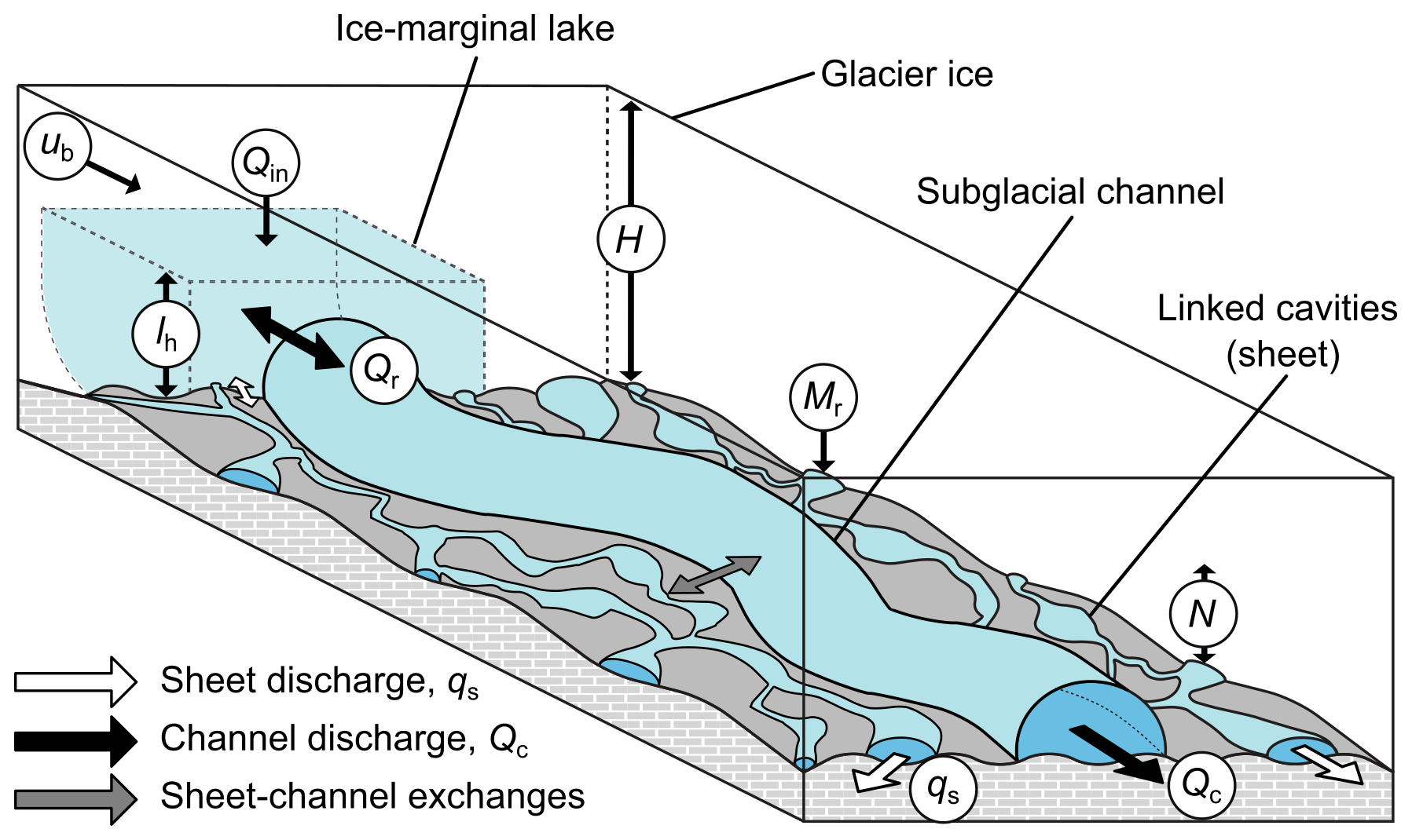
Figure 1 Schematic illustration of our model, showing a glacier (with thickness, H) and ice-marginal lake (with water height, l_h, and water input, Q_in). The lake is connected to a subglacial channel (with scalar discharge, Q_c) and a distributed system of linked cavities (with vector discharge q_s) fed by a basal melt term (M_r). Changes in l_h modifies Q_c and q_s which in turn changes basal ice velocity, U_b through effective pressure, N. Although the lake is shown here to connect with one channel, any number of connections can be specified during model set-up.

2.1 Ice flow and subglacial drainage models

GlaDS (Werder et al., 2013) is a widely used 2D continuum model of subglacial hydrology (Dow et al., 2018; McArthur et al., 2023; Hayden and Dow, 2023; Hepburn et al., 2024; Ehrenfeucht et al., 2025). It operates on an anisotropic mesh and includes a description of (i) distributed flow through a linked-cavity network system represented as a continuous sheet with variable thickness, and (ii) channelised flow through Röthlisberger channels that are located along element edges. Sheet elements exchange water with channels, and the cross-sectional area of these channels evolves through time due to the dissipation of potential energy, sensible heat exchange, and cavity closure rates due to viscous ice creep. Discharge in both the distributed (q_s, m² s⁻¹) and channelised system (Q_c, m³ s⁻¹) is driven by gradients in the hydraulic potential, ∇ϕ (Pa m⁻¹), with steeper hydraulic gradients driving enhanced water discharge. In GlaDS, Q_c is always non-zero along every internal edge, though few reach a discernible discharge. For ease of visualisation we follow Werder et al. (2013) in declaring edges where $Q_{\mathrm{c}}\ge \mathrm{1}{\mathrm{m}}^{\mathrm{3}}{\mathrm{s}}^{-\mathrm{1}}$ to be `meaningful channels' (e.g., Fig. 2c–e). Water in the distributed and channelised drainage components is assumed to be at the pressure melting point. An advantage of GlaDS for simulating jökulhlaup pathways is that the location of these meaningful channels is automatically determined and may evolve throughout a simulation without prior prescription: a behaviour not represented in previous 1D jökulhlaup models. Boundary conditions are applied in GlaDS either as a prescribed flux (typically for upstream inflow boundaries) or ϕ (for downstream outflow boundaries). We refer interested readers to Appendix A1 for an overview of key GlaDS equations, and to Werder et al. (2013) for a full description.

ISSM is a finite element higher-order ice-flow model which operates on anisotropic meshes and can be coupled to additional modelling components such as GlaDS (Larour et al., 2012). In addition to the ice-marginal lake modifications, which we describe below (Sect. 2.2), the primary difference between the original GlaDS (Werder et al., 2013) and the ISSM version used here (Ehrenfeucht et al., 2023) is that rather than assuming water flow within the continuous sheet to be turbulent (cf. Werder et al., 2013), we allow it to switch freely between laminar and turbulent flow according to the local Reynolds number, by implementing the Hill et al. (2024) transition parameterisation. We also prevent cavity expansion by ice creep when effective pressure, N<0 Pa ($N=p_{\mathrm{i}}-p_{\mathrm{w}}$, where p_i is ice pressure and p_w is water pressure) because GlaDS does not include mechanisms to represent uplift of basal ice (separation at the ice-bed interface) once water pressure exceeds ice overburden (e.g., Tsai and Rice, 2010; Schoof et al., 2012; Dow et al., 2015). Without a physical representation of uplift, allowing cavity expansion by ice creep when N<0 Pa is undesirable and has been shown to inhibit channel formation in overpressurised regions of the bed (Hill et al., 2024).

To capture the influence of ice-marginal lake drainage on basal sliding, we include a two-way coupling between ice flow and subglacial hydrology. The GlaDS-derived effective pressure N modifies basal velocity U_b (m a⁻¹) by governing frictional resistance at the ice-bed interface. In turn, the magnitude of U_b modifies the rate at which cavities open and thereby controls the thickness of the sheet (Eqs. A7–A8). These interactions featured in the Kingslake and Ng (2013) model, but the use of ISSM–GlaDS here enables the resulting ice-dynamical variations to be fully captured in 2D. As in the model of Kingslake and Ng (2013), we assume water is at the pressure melting point.

Coupling between ISSM and GlaDS is a relatively new development, and the influence of basal friction parameters remains the subject of ongoing research (e.g., Khan et al., 2024; McArthur et al., 2026), though model response is known to be strongly influenced by the choice of friction law (Choi et al., 2023). We view this work as necessarily explorative, and do not undertake a full analysis of the modelling interactions between subglacial hydrology and ice dynamics. Rather, we seek to capture the broad influence that ice-marginal lake drainage cycles have upon ice dynamics. Accordingly, we present results using two widely applied friction laws: (i) a “Budd-style” friction law (Budd et al., 1984) and (ii) “Schoof-style” friction law (Schoof, 2005; Gagliardini et al., 2007). The Budd-style friction law is implemented in ISSM in terms of basal stress with the form:

$$\begin{array}{}\text{(1)}& {\mathit{\tau }}_{\mathrm{b}}=C_{\mathrm{b}}^{\mathrm{2}}{N}^{\mathrm{r}}{U}_{\mathrm{b}}^s,\end{array}$$

where τ_b is the basal stress magnitude (Pa), C_b is the Budd friction coefficient, N is effective pressure, U_b is basal velocity magnitude (the modulus of U_b), and both r and s are friction coefficients. The Schoof-style friction law is implemented in ISSM with the form:

$$\begin{array}{}\text{(2)}& {\mathit{\tau }}_{\mathrm{b}}={\displaystyle \frac{C_{\mathrm{s}}^{\mathrm{2}}{U}_{\mathrm{b}}^m}{{\left(\mathrm{1}+{\left(\frac{C_{\mathrm{s}}^{\mathrm{2}}}{C_{max}N}\right)}^{\mathrm{1}/m}{U}_{\mathrm{b}}\right)}^m}},\end{array}$$

where C_s is the Schoof friction coefficient (note that $C_{\mathrm{s}}^{\mathrm{2}}$, rather than C_s itself, is used to ensure a positive number when inverting for basal friction), m is a friction law exponent $m=\mathrm{1}/n$, and C_max is Iken's bound. In our experiments on a synthetic domain we use the Budd-style friction law (Eq. 1, Sect. 3) to facilitate comparison to the Kingslake and Ng (2013) model. In the Greenland experiment (Sect. 4), with an observational constraint on U_b, we use the Schoof-style friction law (Eq. 2). A Schoof-style friction law has been shown to more faithfully represent observed ice-dynamics with a GlaDS derived N than the Budd-style friction law (McArthur et al., 2023). Following McArthur et al. (2023), and Ehrenfeucht et al. (2023), we limit N to ≥ 3 % of ice overburden pressure with both friction laws to prevent instabilities as N→0 Pa.

2.2 Lake evolution

In our model, a lake is defined as a specific Dirichlet boundary condition (see below) at n vertices along the boundary of the ice-lake contact. As in previous studies (e.g., Kingslake and Ng, 2013), the lake depth, l_h (m, Fig. 1), evolves according to the continuity equation:

$$\begin{array}{}\text{(3)}& {\displaystyle \frac{\mathrm{d}{l}_{\mathrm{h}}}{\mathrm{d}t}}={\displaystyle \frac{\mathrm{1}}{A_{\mathrm{L}}}}[Q_{\mathrm{in}}-Q_{\mathrm{r}}],\end{array}$$

where A_L is the lake area (m²), Q_in (m³ s⁻¹) represents extraglacial lake input (e.g., rainfall, surface runoff) and Q_r (m³ s⁻¹) represents outflow from the lake (when Q_r is negative there is inflow into the lake). Here, we also include the water exchange between the lake and the sheet (unlike Kingslake and Ng, 2013, who isolated cavities from the lake), so that Q_r is given by:

$$\begin{array}{}\text{(4)}& Q_{\mathrm{r}}\left(t\right)=\sum _{i=\mathrm{1}}^n\left({\mathit{q}}_{\mathrm{s},i}\left(t\right)+Q_{\mathrm{c},i}\left(t\right)\right),\end{array}$$

or the sum of the normal component of the continuous sheet discharge q_s, integrated along the ith boundary edge, q_s,i (m³ s⁻¹), and channel discharge, Q_c,i at the ice-lake contact vertices. As a boundary condition at and between vertices along the ice-lake interface, hydrostatic lake pressure fixes the hydraulic potential, ϕ_contact to be:

$$\begin{array}{}\text{(5)}& {\mathit{\varphi }}_{\mathrm{contact}}\left(t\right)={\mathit{\rho }}_{\mathrm{w}}g{z}_{\mathrm{b}}+{\mathit{\rho }}_{\mathrm{w}}g{l}_{\mathrm{h}}\left(t\right),\end{array}$$

at all times, where g is gravitational acceleration (m s⁻²) and z_b is bed elevation ($\mathrm{m}\mathrm{a}.\mathrm{s}.\mathrm{l}.$). Therefore, lake filling/draining alters ϕ_contact and thus ∇ϕ and sheet/channel discharge along the ice-lake contact boundary (see Eqs. A5 and A15). Between neighbouring vertices which do and do not describe an ice-lake-contact boundary, the value of the Dirichlet boundary condition is interpolated. In the case of an ice–lake contact defined on a single vertex (as in the synthetic experiments described below), the sheet discharge in Eq. (4) is integrated over the combined half-edge length either side of the ice–lake contact. This maintains consistent dimensions (flux per unit length) and avoids double-counting in assembly. Finally, because GlaDS assumes that subglacial water temperatures are equal to the pressure melting point, we assume that the lake water also exists at the pressure melting point. The consequences of this decision are explored in Sect. 5.3.

2.3 Method of numerical solution

At each new timestep, we solve for l_h using a Picard fixed-point iteration scheme comprising an outer and inner loop. In the outer loop, we integrate Eq. (3) forward in time to estimate l_h at the current (i.e., new) timestep given the current estimate of Q_r (initialised from the previous timestep), using this l_h to set ϕ_contact. In the inner loop, GlaDS solves for the domain-wide ϕ until it satisfies a set convergence criteria, updating N as it does so (Werder et al., 2013; Hill et al., 2024). Following the inner loop converging, and given the estimated field of ϕ (X,Y), the model updates h_s, Q_c, and q_s, before summing Q_c and q_s at lake boundary nodes to give a new estimate of Q_r (Eq. 4). The outer loop iterates until the maximum pointwise change in l_h between successive iterations falls below a prescribed absolute tolerance.

3 Model application to a synthetic domain

First, we conduct synthetic simulations with the model to establish its consistency with Kingslake and Ng (2013), and to further develop their work. We use a 10 × 3 km rectangular domain (Fig. 2c–f), discretised on a 2D triangular mesh with a characteristic edge length of 100 m (n_vertices=2486). The bed elevation, z_b is characterised by a gentle slope (sin =0.0075) dipping towards the terminus, and ice thickness follows a parabolic profile that increases from H=50 m at X=0 km to H≈155 m at X=10 km. The simulations here are aimed at facilitating comparison with those of Kingslake and Ng (2013), so we use a similar domain as theirs, which was chosen to be loosely analogous to the Merzbacher Lake and South Inylchek Glacier, Kyrgyzstan (Ng and Liu, 2009). An ice-marginal lake with A_L=5 km² is connected to the glacier at a single upglacier boundary vertex $(X,Y)=(\mathrm{10},\mathrm{1.5}$ km), isolating the rest of the lake margin from the subglacial drainage system. This is necessary because Kingslake and Ng (2013) coupled the lake to a single flood channel only and did not couple the adjacent linked cavity system to the lake.

Model variables are given in Table B1 and our synthetic model parameters are given in Table 1. The parameter dependency of GlaDS has been explored extensively (e.g., Dow et al., 2016, 2020; Hill et al., 2024). We limit our sensitivity experiments in Sect. 3.2 below to parameters regarded as critical to subglacial drainage and known to be the largest sources of uncertainty in subglacial hydrology models (Werder et al., 2013; Hill et al., 2025a, b). These include the channel and sheet conductivity terms k_c and k_s, which govern how easily water is transmitted through the system (i.e., a hard-bedded glacier might be expected to have a higher conductivity than a soft-bedded glacier Dow, 2022); and the terms controlling the geometry of linked cavities such as the basal bump height, h_b, the channel sheet width, l_c, and the cavity spacing, l_r. We also vary the terms controlling water input to the subglacial system, via the basal melt rate M_r, and to the lake, via the lake refill rate, Q_in, which is held constant through time in the synthetic experiments. A reference simulation is conducted at the mid-range values of these parameters as listed in Table 1. Then, as is common practice (Dow, 2022), we vary one parameter at a time between a minimum and maximum bound (Table 1; informed both by previous work and the limits of numerical stability), in additional runs (Fig. 3).

Each simulation is run from t=0 to 15 years at 30 min timesteps. We use a Budd-style friction law (Eq. 1) with C_b=100, $r=\mathrm{1}/\mathrm{4}$, and $s=\mathrm{1}/\mathrm{4}$. This gives units for C_b of ${\mathrm{kg}}^{\mathrm{3}/\mathrm{8}}{\mathrm{m}}^{-\mathrm{1}/\mathrm{2}}{\mathrm{s}}^{-\mathrm{5}/\mathrm{8}}$ and was chosen to be consistent with Bindschadler (1983) and Kingslake and Ng (2013). The ice dynamic model is initialised with ${\mathit{U}}_{\mathrm{b}}=(-\mathrm{100},\mathrm{0})\mathrm{m}{\mathrm{a}}^{-\mathrm{1}}$, with Dirichlet boundary conditions (${\mathit{U}}_{\mathrm{b}}=(\mathrm{0},\mathrm{0})\mathrm{m}{\mathrm{a}}^{-\mathrm{1}}$) at the glacier terminus and stress-free Neumann boundary conditions elsewhere. Following Hill et al. (2024), the hydrology model is initialised with ϕ equivalent to 90 % of ice overburden pressure, and an initial sheet thickness h_s equal to half the bump height h_b. At the terminus, we prescribe ϕ to be ≈ 1 ×10⁴ Pa as our GlaDS Dirichlet boundary condition. Though arbitrary, this does not qualitatively affect the results. We impose zero water inflow as our Neumann boundary condition along the other three upglacier boundaries. The ice-marginal lake has an initial water height of 30 m (l_h at t=0). The evolution of the reference case through time is shown in Fig. 2, and the sensitivity of lake height l_h, flood discharge Q_r, and basal velocity magnitude U_b through time is shown in Figs. 3 and 4.

Table 1 Model parameters in our synthetic experiments. The parameters we vary are highlighted in bold, with the reference case value given first and the range over which they vary in parentheses.

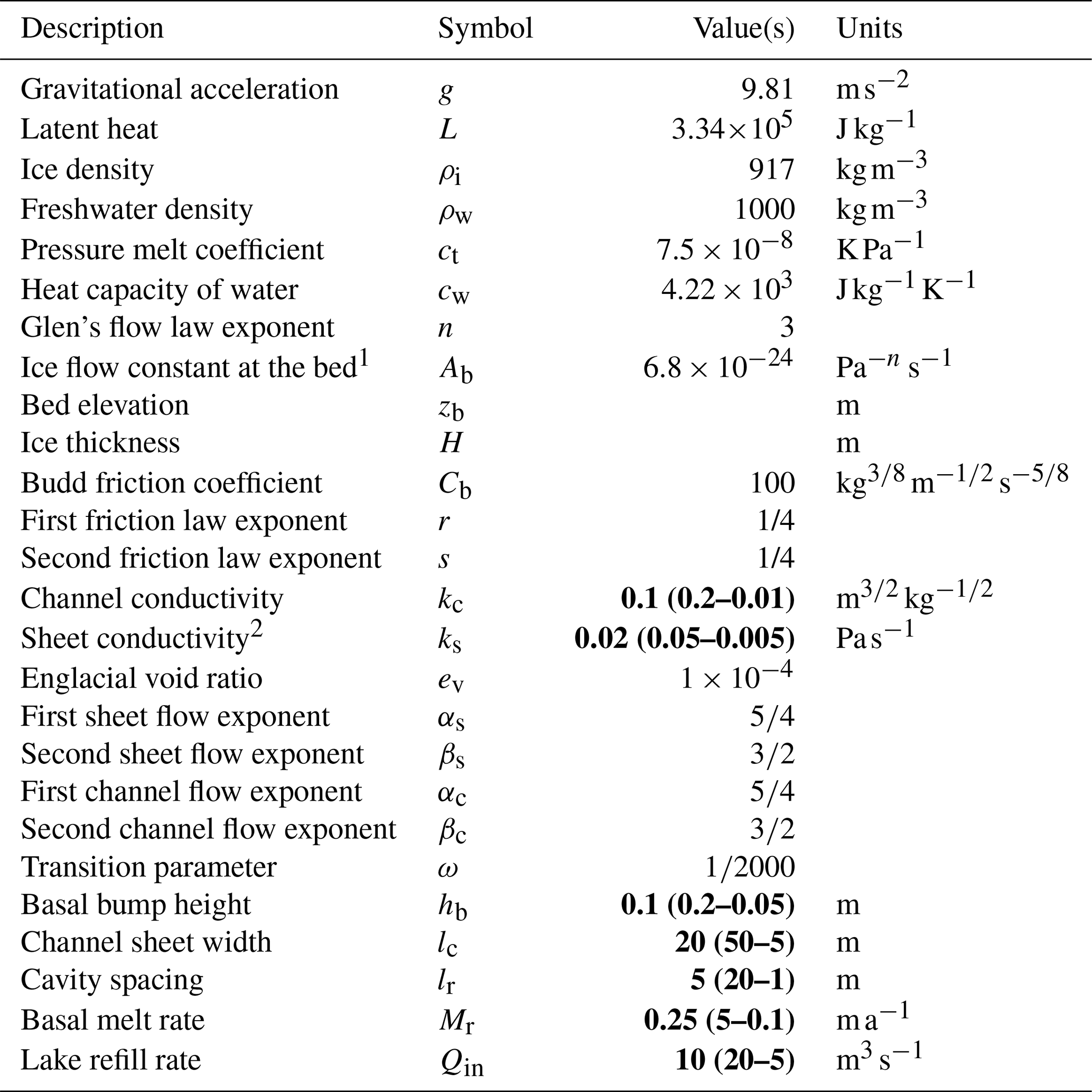
¹ The bed is assumed to be at pressure melting point, but the ice column is assumed equivalent to −10 °C or $A=\mathrm{4.9}\times {\mathrm{10}}^{-\mathrm{25}}$ Pa⁻ⁿ s⁻¹. ² Following Hill et al. (2024) the units for k_s differ from those given by Werder et al. (2013).

3.1 Stable flood cycles

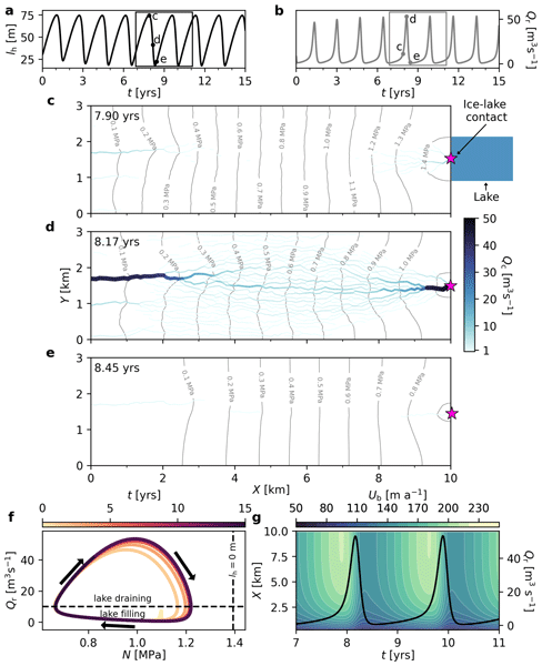
In the reference simulation, the lake undergoes recurrent, stable, and asymmetric fill-drain cycles (Fig. 2a). Drainage is associated with a recurring flood with stable maximum amplitude and duration (Fig. 2b). The lake only partially drains in each flood cycle, and never reaches a height necessary to sustain flotation (N=0 Pa, Fig. 2f). In the initial 5 years of transient evolution, when the model adjusts to initial conditions, peak flood discharge increases with each successive flood, and the lake reaches successively lower post-flood lowstands (Fig. 2a, b). Thereafter, the flood cycles reach a stable periodicity and clockwise hysteresis (Fig. 2f) with flood cycles occurring approximately every 1.5 years. As will be discussed in Sect. 5, these simulated cycles are comparable to – yet with notable differences from – those of Kingslake and Ng (2013).

The evolution of the subglacial channel system through a single flood cycle is shown in Fig. 2c–e (an animated version is shown in Movie A1), and the width-averaged basal velocity response over the same flood cycle and the following one is shown in Fig. 2g. At the start of a flood cycle (Fig. 2c), as the lake approaches its highstand, channelised drainage is limited and ∇ϕ is controlled by the ice surface slope. Close to the ice–lake contact ($X>\mathrm{9},\mathrm{km}$), contours of hydraulic potential form ridges pointing downglacier from the ice–lake contact. In GlaDS, sheet discharge, q_s, is directed perpendicular to these contours of ∇ϕ and such ridges would induce sheet flow out of the lake. Four short (< 100 m), low-discharge (≥ 1 m³ s⁻¹) channels remain open following formation during the previous flood cycle, three at the terminus and one at the ice–lake contact.

During the lake filling phase, increasing l_h drives ϕ_contact up (Eq. 5), resulting in a steeper ∇ϕ across the domain and promoting channelised drainage close to the ice–lake contact (Movie A1). During the lake drainage phase, initiated once Q_r begins to rapidly exceed the lake refill rate, Q_in (when l_h≈75 m and t≈7.9 years), an arborescent channel structure originating from the lake extends across the full y-axis extent of the domain, perpendicular to the contours of ϕ, and deviating from the direction of ice-surface slope. Simultaneously, channels extend upglacier from the terminus, and contours of ϕ become increasingly convex downglacier. At the flood peak, channel tributaries coalesce into the three primary terminus channels which evacuate water from the system. As the lake level drops sharply during a flood, ϕ_contact drops, reducing ∇ϕ, and in turn reducing Q_c below the level necessary to sustain channels across the domain, including at the ice–lake contact. Once Q_r<Q_in the flood terminates and the cycle begins again. Each cycle takes ≈ 1.5 years with the rising and falling limb of the flood lasting ≈ 6 months.

Basal velocity, U_b changes significantly during a flood cycle (Fig. 2g), tracking the development of a significant channelised drainage system. The glacier accelerates during the year-long flood initiation phase before channelised drainage is widely established, then decelerates abruptly (in less than two months) as channels become well-established, approximately two months before the flood peak (Fig. 2g). Ice flow acceleration propagates from the ice–lake contact towards the terminus, with maximum velocity sustained within 2 km of the ice–lake contact.

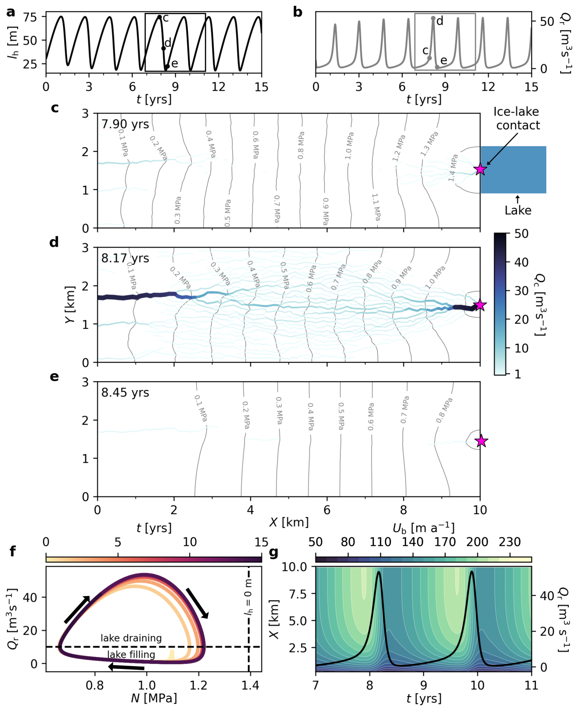
Figure 2 Evolution of the “reference” experiment in our synthetic modelling domain. (a) Lake water height, l_h through time. Black points indicate l_h in panels (c)–(e). (b) Total discharge at the ice–lake contact, Q_r through time. Grey points indicate Q_r in panels (c)–(e) the grey box indicates the time span of panel (g). (c–e) Channel discharge, Q_c at t=7.90 years (c), 8.17 years (d) and 8.45 years (e). In each panel, hydraulic potential ϕ is shown as grey contours, and the ice–lake contact is marked by a magenta star. In panel (c), a representative lake is plotted, though this is not to scale. (f) Phase-plane diagram showing the evolution of Q_r and N through time at the ice–lake contact. Arrows and shading indicate the direction of time. The horizontal dashed line denotes the lake refill rate, Q_in=10 m³ s⁻¹. The vertical dashed line indicates N when l_h=0 m. (g) Filled contour plot showing the across-flow averaged velocity through time. White contours represent velocity at 10 m a⁻¹ intervals and the black line shows Q_r between years 7–11.

3.2 Parameter sensitivity

Figure 3 plots the time series of lake height l_h and lake discharge Q_r from a total of 14 simulations across the maximum (red lines) and minimum (blue lines) parameter values, with the reference “mid-point” simulation in grey. The majority of simulations yield stable and recurring asymmetric lake filling and drainage cycles (Fig. 3a(i)–f(i)) with corresponding variations in Q_r at the ice–lake contact (Fig. 3a(ii)–f(ii)). The parameter variations most strongly influence the amplitude of lake height and its rate of change, both of which influence the timing of flood initiation and peak flood discharge, with higher amplitude lake depth cycles leading to higher peak flood discharges (Ng and Björnsson, 2003).

Increasing channel conductivity, k_c, in effect making channels more sensitive to ∇ϕ (see Eq. A15), leads to lower lake highstands as the lake drains sooner. However, peak discharge is higher as the lake also drains more quickly and drains entirely. At maximum k_c, there is a longer transient before the model reaches a fixed flood recurrence interval, draining at a higher frequency than the default value of k_c until ∼ 11 years into the simulation, at which point flood cycles occur at approximately the same interval as in the default case (Fig. 3a(ii)). Conversely, at minimum k_c, the capacity of channels to drain the lake is inhibited and flood onset is delayed. Because channels grow slowly, peak Q_r is also dampened, leading to relatively long flood recurrence intervals (∼ 4 years, Fig. 3a(ii)).

Increasing the sheet conductivity, k_s increases the capacity of the sheet to accommodate water and delays transmission to channels. This results in reduced lake highstands and delayed flood initiation as the onset of classical channel growth is delayed. Reducing k_s increases the relative efficiency of channels and leads to more higher amplitude lake-fill drain cycles (Fig. 3b(i)), with shorter and higher discharge floods as a result (Fig. 3b(ii)). Changing h_b has a similar effect to reducing k_s, although at the maximum bump height the sheet becomes so efficient that it can accommodate all lake discharge and within 1 year the lake reaches a stable equilibrium where Q_r=Q_in (Fig. 3c(i)).

Changing the contributing width of the sheet to the channel (l_c) or the representative horizontal spacing of cavities (l_r) alters the relative efficiency of channelised and sheet drainage. Reducing l_r and increasing l_c reduces the lake highstand and lowers peak discharge, and vice versa when increasing l_r and reducing l_c. Finally, increasing the input of water into either the glacier via basal melt rate, M_r (Fig. 3f) or lake via Q_in (Fig. 3g) enhances the amplitude of l_h oscillations and in turn, peak flood discharge (Fig. 3f).

In all simulations, the maximum lake height remains below the maximum ice thickness (150 m) and does not surpass the effective pressure necessary to initiate ice flotation (N=0 Pa). In most simulations the lake does not reach a lowstand below ∼ 10 m, only draining completely when $k_{\mathrm{c}}=\mathrm{0.2}{\mathrm{m}}^{\mathrm{3}/\mathrm{2}}{\mathrm{kg}}^{-\mathrm{1}/\mathrm{2}}$, and when h_b=0.05 m.

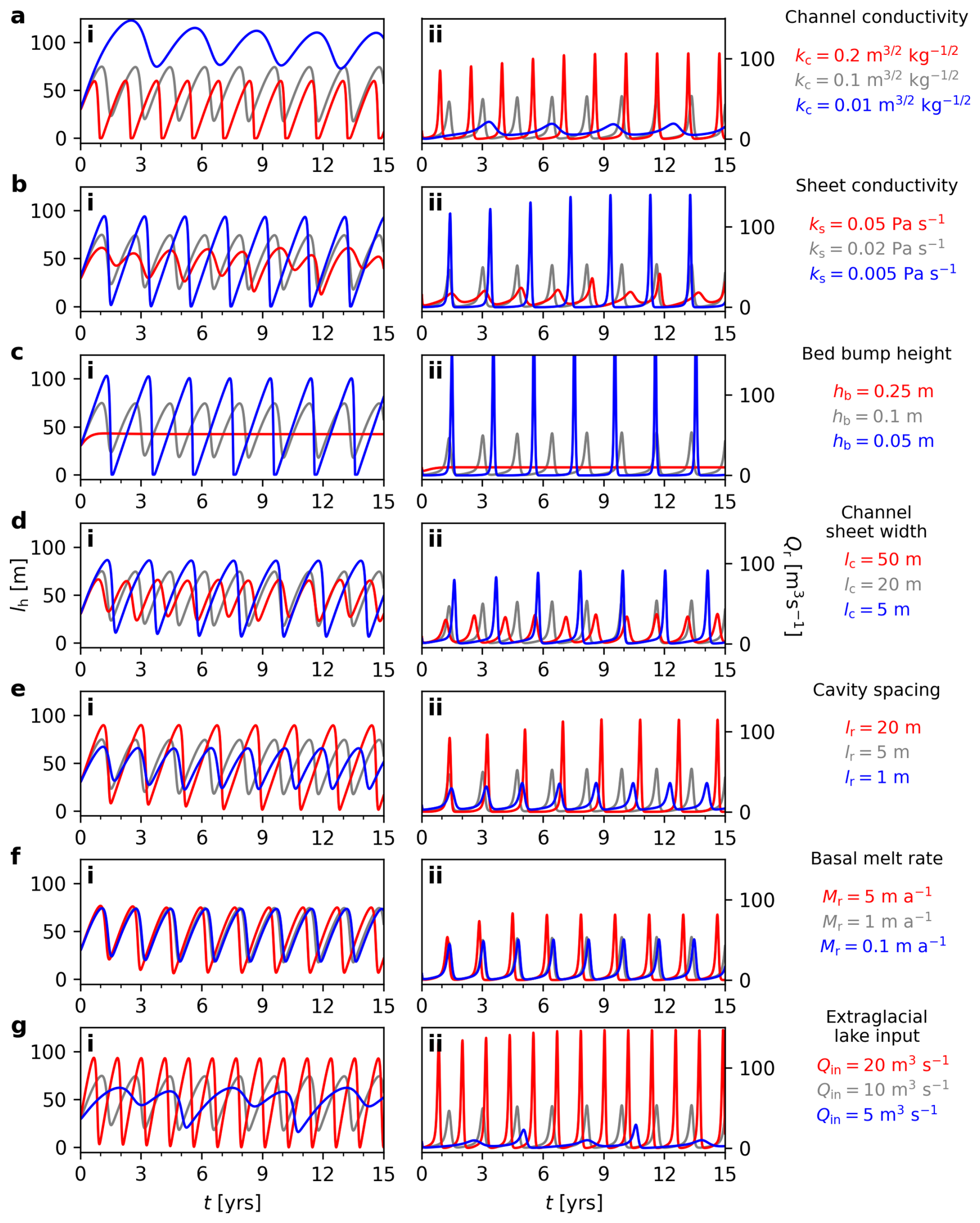
Figure 3 Lake water height, l_h (left panels, i) and sum discharge at the ice–lake contact, Q_r (right panels, ii) across a range of key model parameters. (a) Channel conductivity, k_c. (b) Sheet conductivity, k_s. (c) Basal bump height, h_b. (d) Channel sheet width, l_c. (e) Cavity spacing, l_r. (f) Basal melt rate, M_r. (g) Lake refill rate, Q_in. In all panels, the reference parameter experiment is shown in grey.

The character of the fill–drain cycles has a strong influence on the spatiotemporal pattern of basal sliding across all experiments. In each case, modelled ice motion follows the reference case with velocity peaking before peak discharge is reached, and dropping rapidly thereafter during the falling limb of a flood (Fig. 4). In general, shorter more intense jökulhlaup cycles lead to a more rapid but lower magnitude velocity response (e.g., Fig. 4a, e, f), whereas broad and less intense jökulhlaup cycles yield more gradual but higher magnitude velocity responses for a longer duration (e.g., Fig. 4b, d). The highest magnitude basal velocity ($>\mathrm{300}\mathrm{m}{\mathrm{a}}^{-\mathrm{1}}$) is associated with the low k_c case (Fig. 4d), characterised by muted lake filling–drainage cycles but a relatively high lake level (Fig. 3a(i)).

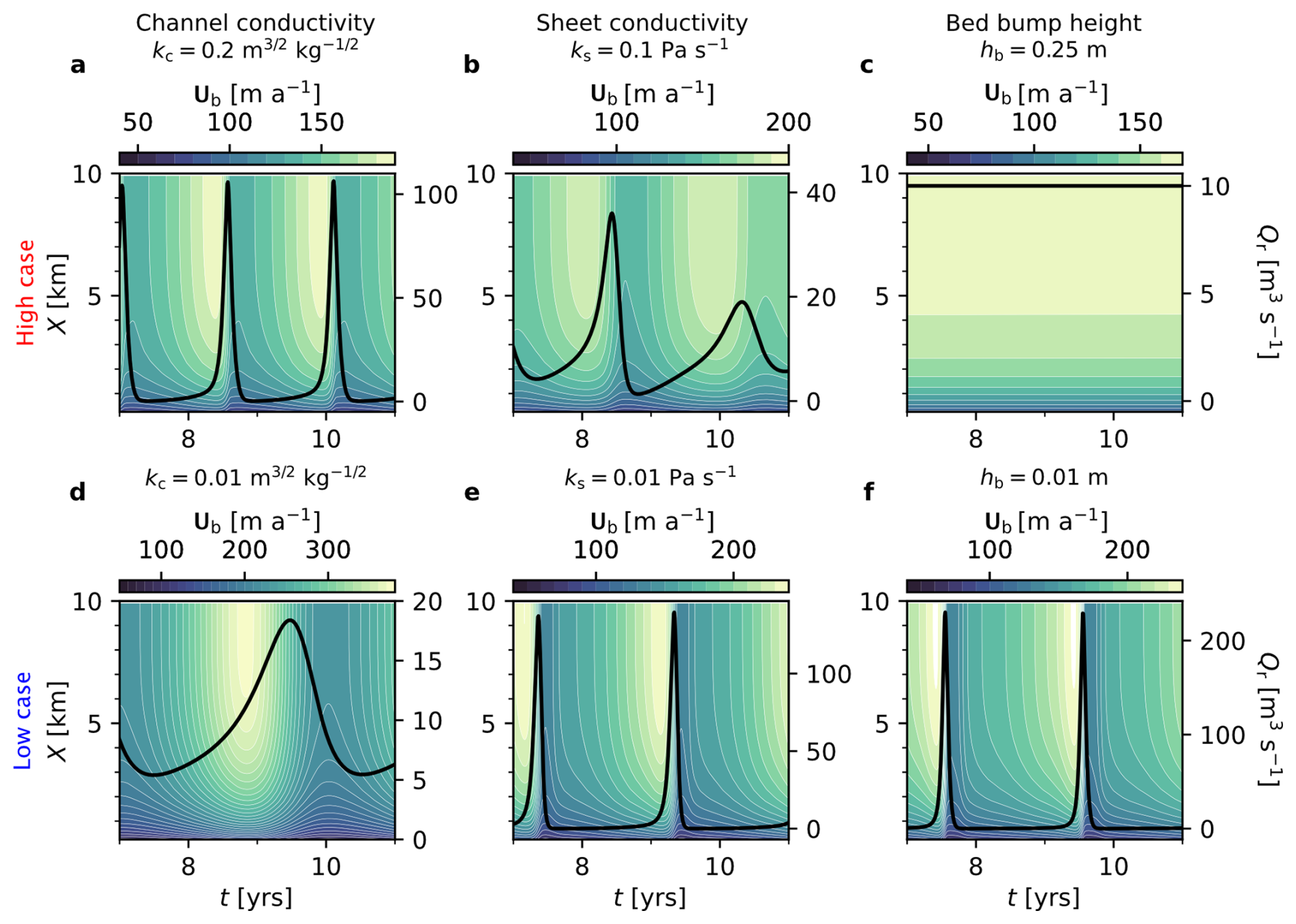
Figure 4 Across-flow velocity through time for key GlaDS parameters in the synthetic experiment. (a–c) The high channel conductivity (k_c, a), sheet conductivity (k_s, b), and bump height (h_b, c) cases. (d–e) The low k_c (d), k_s (e), and h_b (f) cases. In each panel, white contours represent velocity (every 10 m a⁻¹) and the black line shows Q_r between years 7–11. Note, the limits of the colourbar vary with each plot.

4 Model application to Isunnguata Sermia, Greenland

Isunnguata Sermia is a land-terminating outlet glacier draining a catchment of ≈16 000 km² on the western margin of the Greenland Ice Sheet (Fig. 5a–c). Its terminus region is characterised by a deep bedrock trough running parallel to flow, which anabranches ≈ 20 km from the ice margin (Fig. 5c). The glacier terminates into a sub-aerial proglacial river system (McCerery et al., 2026). An ice-dammed lake ≈3 km² in area, and ≈100 m deep (Livingstone et al., 2026) abuts the northern margin of Isunnguata Sermia's tongue (Fig. 5). The lake drains subglacially with a periodicity of 1–3 years, having undergone at least 12 fill-drain cycles between 1987–2024 (Livingstone et al., 2026, Fig. 5g). There are two ice-contact boundaries between Isunnguata Sermia and the ice-marginal lake, a prominent ice cliff boundary along the western margin of the lake through which the lake drains, and an intermittent boundary along the eastern margin that receives drainage from the glacier through an emerging subglacial stream during lake lowstands, and becomes ice-contact at lake highstands (Livingstone et al., 2026).

4.1 Model setup

We discretise our Isunnguata Sermia domain (derived from Lindbäck et al., 2015) using an anisotropic mesh with an edge length of 150 m close to terminus, increasing to 2 km close to the upper margin of our domain at the approximate ELA (at H≈1600 m). The mesh is further manually refined to a typical edge length of 50 m close to the ice-marginal lake (Fig. 5c) in order to faithfully represent glacier geometry close to the ice margin. Bedmachine v5 is used for z_b and H (Morlighem et al., 2017, 2022, Fig. 5b, c). Our domain is clipped to exclude areas of the glacier where H<100 m to ensure numerical stability. Basal velocity, U_b, is initialised from the 2021 MEaSUREs annual surface velocity mosaic (Joughin et al., 2015). Geothermal heat flux is taken from Shapiro and Ritzwoller (2004), and basal melt rates are taken from Karlsson et al. (2021). The flow-law rate factor A within the ice-column is derived using surface ice temperatures from Ettema et al. (2009) and assuming a temperature-dependent Arrhenius relation following Cuffey and Paterson (2010).

Our model includes multiple boundary conditions in order to represent Isunnguata Sermia. For the hydrological solution, we impose two distinct Dirichlet boundary conditions at three locations: (i) at the two ice–lake contact boundaries ϕ_contact is allowed to evolve with l_h (see Eq. 5) and (ii) a fixed atmospheric boundary is imposed at the glacier terminus. At all other vertices, we impose Neumann (zero-inflow) boundary conditions. The ice–lake contacts are manually delineated: seven vertices were identified at the western lake boundary and at the eastern margin we identified the lowest elevation vertex within a group of vertices close to the observed stream. At all ice-lake contact vertices we fix bed elevation equal to the minimum lake elevation (257.9 m a.s.l.). Because our model assumes a fixed lake area (A_L=3 km²) and cannot dynamically represent intermittent lake-glacier contact along the eastern margin, prescribing the same boundary conditions at the eastern ice–lake contact as along the western ice–lake contact provides a simple and consistent boundary treatment and ensures water can exchange between the subglacial system and the lake at both places. At the glacier terminus we set the Dirichlet boundary condition ϕ equal to atmospheric pressure at the lowest elevation boundary vertex (cyan triangle in Fig. 5c). Within the ice-dynamic solution, the boundary condition velocity is given by the initialisation U_b (Dirichlet), except at the western ice–lake contact where velocity is allowed to evolve freely (Neumann).

Model simulation necessitates knowledge of the spatial field of basal friction coefficient, C, which we assume to be time-invariant. Because we have an observational constraint on ice-surface velocity, we use a Schoof-style friction law (see Eq. 2, Sect. 2.1), inverting for the basal friction coefficient C_s using an L-curve scheme following Wolovick et al. (2023). We run an initial inversion for C_s using an empirically-derived N (assuming N=p_i), before running a simple GlaDS-only model run over 10 years, which does not include an ice-marginal lake, surface melt or two-way coupling to ice dynamics. This allows us to derive a more realistic and spatially variable estimated field of N from which a second inversion for basal friction can be obtained. Such an approach has previously been demonstrated to yield more faithful basal inversions in a coupled hydrology model (Ehrenfeucht et al., 2023; McArthur et al., 2023).

As climate forcing, we use the 10 km resolution daily Modèle Atmosphérique Régional (MAR, v3.14) runoff and accumulation data (Fettweis et al., 2017) between 2007–2025 inclusive. Runoff is routed directly to the bed at all vertices. Whereas we keep Q_in fixed in the synthetic experiments (Sect. 3), here the extraglacial water input to the lake is likely to vary with time as a function of air temperature (Ng et al., 2007; Ng and Liu, 2009). To account for this, we use a simple temperature index (as in Kingslake, 2015), where Q_in is given by:

$$\begin{array}{}\text{(6)}& Q_{\mathrm{in}}=\left\{\begin{array}{ll}\max (kT,\mathrm{1}),& T>\mathrm{0}\\ \mathrm{1},& T\le \mathrm{0},\end{array}\right.\end{array}$$

where the temperature-index coefficient k is equal to $\mathrm{2}{\mathrm{m}}^{\mathrm{3}}{\mathrm{s}}^{-\mathrm{1}}{\mathrm{K}}^{-\mathrm{1}}$. We set $Q_{\mathrm{in}}\ge \mathrm{1}{\mathrm{m}}^{\mathrm{3}}{\mathrm{s}}^{-\mathrm{1}}$ to capture positive changes in lake elevation observed between melt seasons in Fig. 5g.

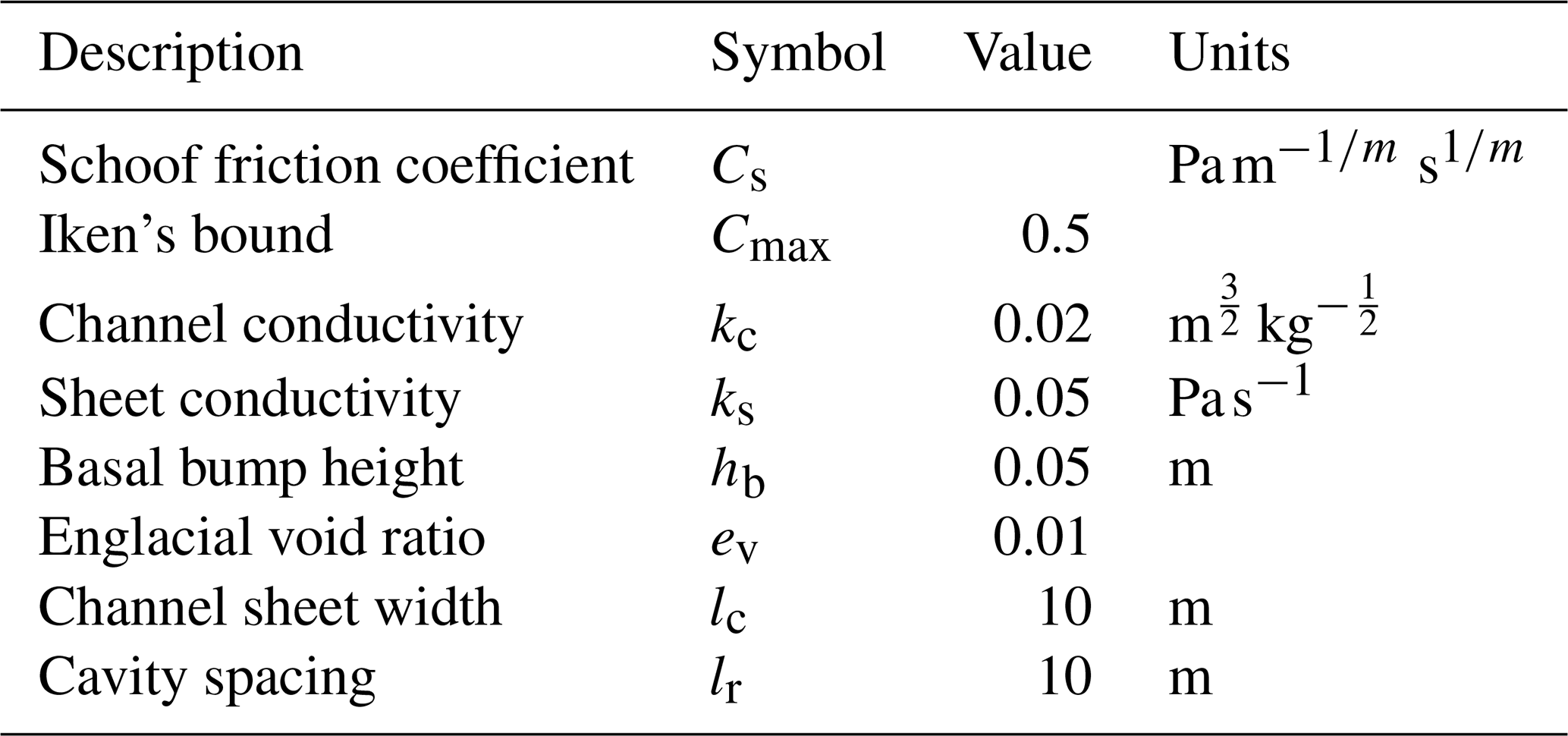
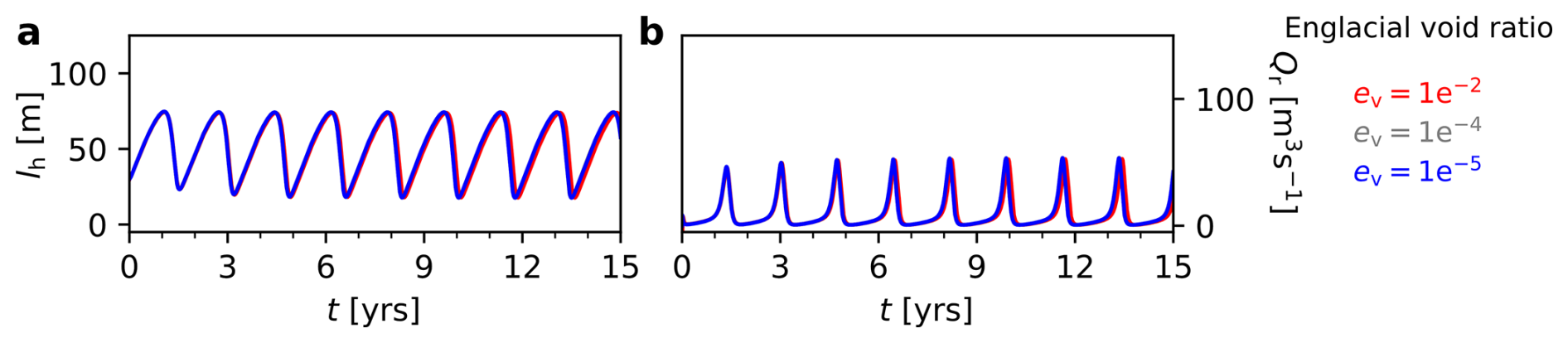
Since our objective is to assess the model's ability to reproduce the observed record of fill-drain cycles of an ice-marginal lake in Fig. 5g, we focus on achieving a simulation that yields the closest quantitative match. Guided by insights from the synthetic experiments (Sect. 3), we choose the final parameters (Table 2) as follows: a decrease in channel conductivity, k_c, to 0.02 ${\mathrm{m}}^{\frac{\mathrm{3}}{\mathrm{2}}}{\mathrm{kg}}^{-\frac{\mathrm{1}}{\mathrm{2}}}$, an increase in sheet conductivity, k_s to 0.05 Pa s⁻¹, a decrease in the basal bump height, h_b to 0.05 m, and changes to both the channel sheet width, l_c, and cavity spacing, l_r to 10 m. Compared to the synthetic case, we also increase the englacial void ratio e_v to 0.01. This has little influence on our synthetic case when tested to the same limits (Fig. C1) because the model does not reach flotation pressures (Sect. 3.1). However, in our Greenland experiments, increasing e_v dampens the model sensitivity to sudden changes in meltwater input to the system and prevents unreasonably high water pressures (> 300 % of overburden pressure) in isolated pockets close to the domain boundary. Across sensitivity tests, parameter variations produce changes in the frequency, timing, and amplitude of modelled outputs without altering the qualitative drainage system behaviour.

Table 2 Parameters in our Greenland run, listing those which differ from Table 1.

We simulate the Greenland model forward in time from 1987 to 2025 (for 38 years at a 5 min timestep). This simulation consists of three phases, the first of which involves running the model (for twenty years of model time) to reach a winter steady state where the 95th percentile difference in sheet thickness between successive timesteps is below $\mathrm{1}\times {\mathrm{10}}^{-\mathrm{6}}\mathrm{m}$. During the steady state phase, we allow the ice-marginal lake to freely evolve from an initial height of l_h=70 m, the mean lake height between 1987–2024 (Livingstone et al., 2026). The steady state phase allows the model to reach a condition approximating the anticipated wintertime hydrological conditions in which there is limited channel activity and water pressures across the domain are close to the flotation fraction (p_w≈0.7–0.9 p_i). We then run a “spin-up” phase from 1997–2007 where we introduce a climate forcing by gradually increasing the 2007 runoff by 10 % each year. Following this spin-up, we run an unconstrained phase from 2007–2025 where we apply the full climate forcing and compare results with the 2007–2025 lake-level record.

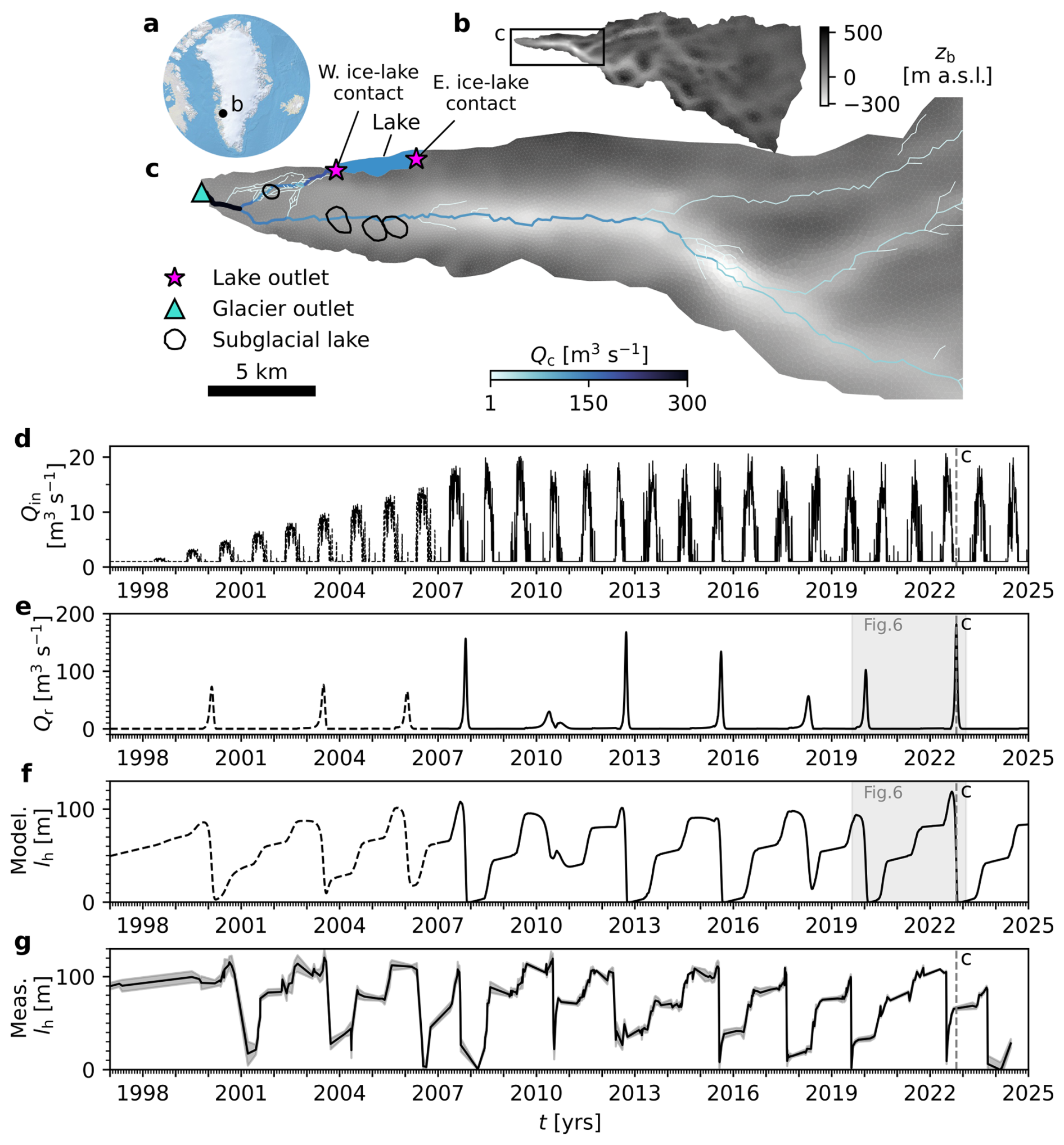
Figure 5 Ice-marginal lake drainage in the Isunnguata Sermia glacier catchment. (a) The location of our model domain (panel b) in West Greenland. (b) Our modelling domain, coloured by the bed elevation (Morlighem et al., 2022), the extent of panel (c) is outlined. (c) Channel discharge, Q_c at the end of the 2018 melt season. The primary drainage axis is located within the along-flow orientated subglacial trough. The location of the two ice–lake contacts and the glacier outlets are marked by a pink star and a cyan triangles respectively. An approximate lake extent is marked within the blue polygon. The location of subglacial lakes 1–3 and Anomaly 1 discussed in Livingstone et al. (2026) are shown in black polygons. (d) Extraglacial lake input, Q_in, during the spinup (dashed line) and transient modelling phase (solid line). Runoff increases by 10 % each year during the spin-up phase (1997–2007). (e) Sum ice–lake contact discharge, Q_r at the ice–lake contacts during the spinup (dashed line) and transient modelling phase (solid line). $Q_{\mathrm{r}}<\mathrm{0}{\mathrm{m}}^{\mathrm{3}}{\mathrm{s}}^{-\mathrm{1}}$ indicates net discharge into the lake, and vice versa when $Q_{\mathrm{r}}>\mathrm{0}{\mathrm{m}}^{\mathrm{3}}{\mathrm{s}}^{-\mathrm{1}}$. (f) Modelled lake height, l_h during the spin-up (dashed line) and unconstrained modelling phase (solid line). (g) Measured l_h and uncertainty values taken from Livingstone et al. (2026). The dashed vertical line in panels (d)–(f) shows the time represented by panel (c), and the shaded grey box indicates the time span shown in Fig. 6.

4.2 Flood cycles in Greenland

The combined spin-up and unconstrained modelling phase is shown in Fig. 5d–g. The spin-up phase (dashed line in Fig. 5d–f) is characterised by three cycles of lake filling and partial drainage, each reaching successively higher lake highstands and having a shorter flood recurrence period than the previous one; these cycles track the development of a catchment-wide subglacial drainage system induced by successively more intense melt summers (Fig. 5d).

From 2007 onwards, once the model is subject to the full extent of annual melt-forcing, the lake repeatedly fills and drains with a recurrence interval between floods of ∼ 2–4 years. At the peak of a flood, using model year 2022 as an example, the simulated drainage system of Isunnguata Sermia is characterised by a channel that occupies the central trough and extends > 45 km upglacier (Fig. 5c). The majority of surface melt is routed through this “primary drainage axis” towards the glacier terminus, and an anabranching tributary system is visible ∼ 20 km upstream. Near the terminus, a second drainage axis, comprising a high discharge central channel and two lower discharge subsidiary channels, connects the western ice–lake contact to the primary drainage axis, converging ∼ 2 km from the terminus.

Each modelled jökulhlaup lasts 3–4 months, far exceeding the typical flood duration of 5–8 d observed at Isunnguata Sermia (Livingstone et al., 2026). Correspondingly, our modelled peak Q_r≈ 100–200 m³ s⁻¹ are markedly lower than that of the 2022 jökulhlaup described by Livingstone et al. (2026), which had an estimated mean discharge of at least 480 m³ s⁻¹ and a likely considerably higher instantaneous peak.

The lake fill–drain cycles are characterised by slow-rising limbs (between jökulhlaups) and abrupt drawdowns (jökulhlaups), though their hydrograph shape is irregular. Lake drainages typically occur at the end of a melt season. Lake levels then remain low during the subsequent winter, before filling in an irregular sawtooth fashion (as in Ng and Liu, 2009), with the lake filling more rapidly during summer melt seasons and remaining stable, or lowering slightly, during the intervening winter period. Lake drainage is triggered following the second or third melt season, and the cycle begins anew.

The timing and water height of modelled lake highstands in our simulation phase align well with those in the observed record, capturing variability in both flood timing and the proportion of lake drainage. Eight lake highstands are evident in the observed record (Fig. 5g) between 2007–2024, seven of which correspond with a simulated lake highstand to within ∼ 2 months and ±20 m (Fig. 5f). Further, there is good overall agreement in the lake lowstand heights, with the model matching observations of partial (e.g., 2010–2011) and complete lake drainage events (e.g., 2007–2008). This match is not perfect (e.g., 2013) and may be influenced by gaps in the observational record (Livingstone et al., 2026).

The evolution of channels during a typical jökulhlaup cycle (2019–2023) is shown in Fig. 6. On reaching lake highstand in 2019, the development of a significant channel connection between the lake and the primary drainage axis initiates a jökulhlaup and the drop in lake level (Fig. 6b). As l_h and ∇ϕ lowers at the western ice–lake contact, the lake draining channel is starved of supply and shuts down by creep closure. At the lake lowstand, once ϕ_contact is close to atmospheric pressure, drainage into the lake from the eastern ice–lake contact begins in summer 2020 (Fig. 6c) and the lake quickly fills to ∼50 m. In the 2021 summer (Fig. 6d) and 2022 summer, no significant channels develop upglacier of the eastern ice–lake contact, and Q_in accounts for the rise in l_h. At the end of the 2022 melt season (Figs. 5, 6e), a relatively high discharge jökulhlaup drains the lake via a series of channels at the wester ice–lake contact and connected to the primary drainage axis. Though seven vertices along the western ice–lake contact are connected to the lake, discharge at the lake boundary is concentrated within a single high-discharge channel. Midway along the flood path, ≈ 2.5 km from the lake, this channel diverges and branches into multiple lower discharge channels running sub-parallel to the main lake-draining channel, a behaviour also evident in the synthetic runs (see Sect. 3 and Fig. 2c–e).

Turning to the simulated basal velocity field, ${\mathit{U}}_{\mathrm{b}}=u_{\mathrm{b}},v_{\mathrm{b}}$, Fig. 7 shows the mean components of u_b and v_b between 2014–2025 and the anomalies, generated by subtracting the overall mean velocity from the mean velocity during a jökulhlaup, associated with the modelled 2022 flood (Fig. 7a–d) and the observed 2023 flood (Fig. 7e–h) from Livingstone et al. (2026). Each velocity field is interpolated onto the same model mesh. The x- (u_b) and y- (v_b) components of modelled basal velocity show a mean value (Fig. 7a, b) that agrees closely with the mean observed velocity (Fig. 7e, f), although our model predicts a higher mean $v_{\mathrm{b}}>\mathrm{50}\mathrm{m}{\mathrm{a}}^{-\mathrm{1}}$ close to the lake margin (Fig. 7b) than the $v_{\mathrm{b}}\approx \mathrm{25}\mathrm{m}{\mathrm{a}}^{-\mathrm{1}}$ observed (Livingstone et al., 2026, Fig. 7f). The modelled and observed lake-drainage anomalies (Fig. 7c, d, g, h) agree well in terms of the overall pattern of slow-down and acceleration, but differ in detail and magnitude. In our model, changes in u_b and v_b during a jökulhlaup are lower in magnitude, and are more spatially restricted than observed (Fig. 7). During a modelled jökulhlaup, u_b decreases (corresponding to a westward acceleration) by 20 m a⁻¹ upglacier of the lake, and v_b increases (corresponding to a northward acceleration) by $\approx \mathrm{15}\mathrm{m}{\mathrm{a}}^{-\mathrm{1}}$, with the acceleration restricted to close to the lake boundary (Fig. 7d). In contrast, the observations indicate a more widespread westward acceleration across the full extent of the glacier tongue during a jökulhlaup, with u_b decreasing by $>\mathrm{100}\mathrm{m}{\mathrm{a}}^{-\mathrm{1}}$, and a northward component where v_b increases by $>\mathrm{100}\mathrm{m}{\mathrm{a}}^{-\mathrm{1}}$ towards the lake (Fig. 7). The observed v_b is also more spatially variable than the equivalent model output, with ice accelerating towards the ice-marginal lake across a more extensive portion of the lake-adjacent glacier. Observations additionally identify a southward acceleration in v_b close to the glacier terminus that is not reproduced in our model.

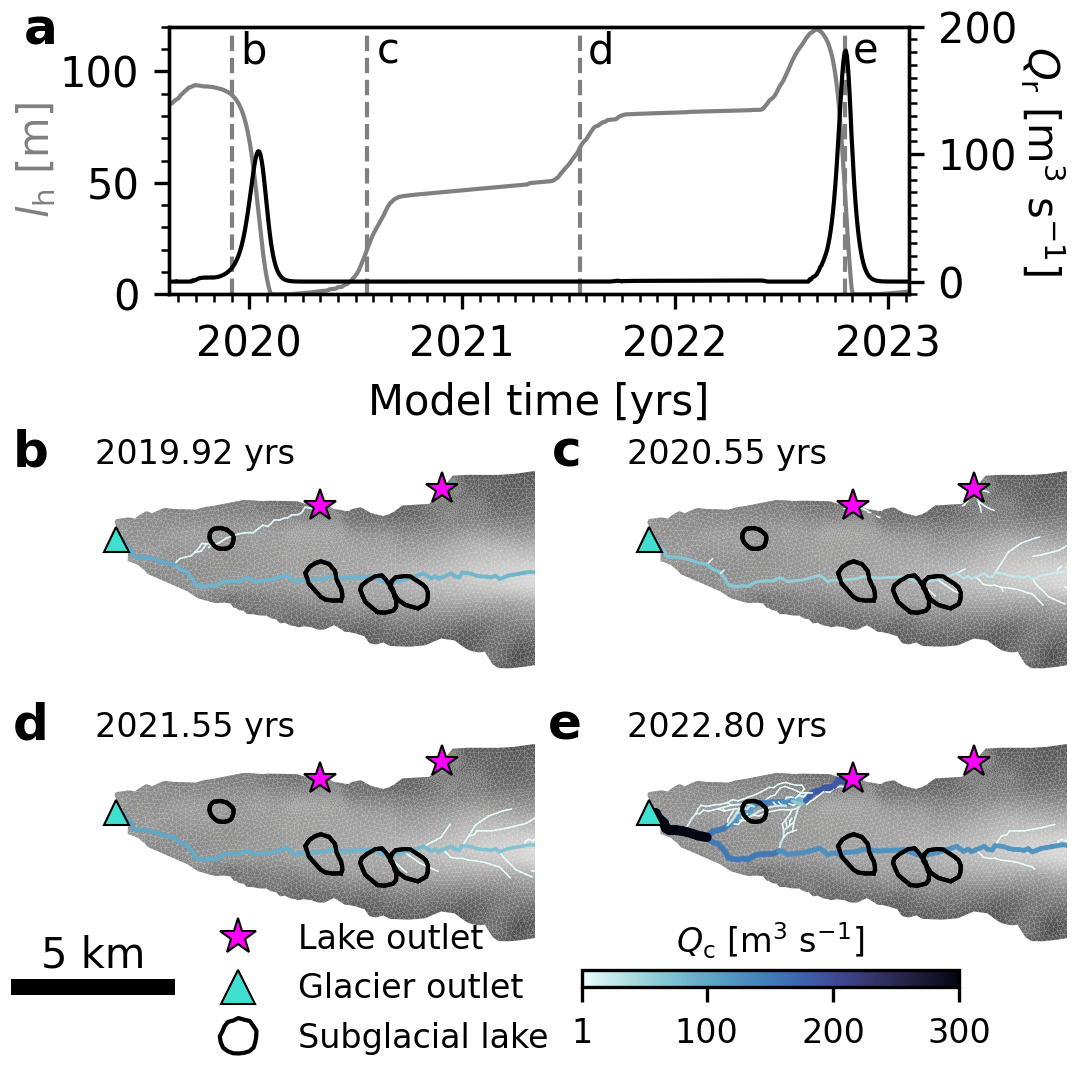
Figure 6 Channel development during a complete lake filling–drainage cycle. (a) Lake height, l_h and flood discharge, Q_r through time. (b–e) Snapshots of channel discharge, Q_c through time, with the location of ice–lake contacts and the glacier outlet marked by pink stars and a cyan triangle respectively. The location of subglacial lakes 1–3 and Anomaly 1 discussed in Livingstone et al. (2026) are shown in black polygons. Dashed lines in panel a indicate the snapshot times in panels (b)–(e).

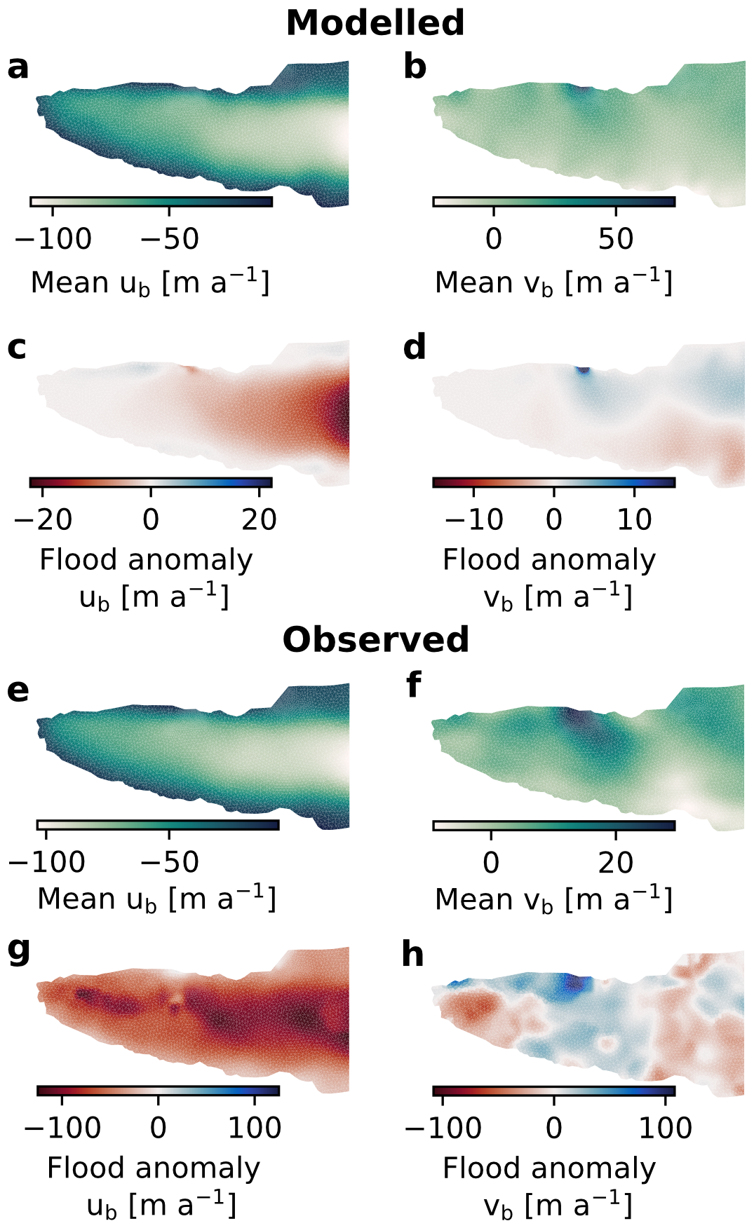
Figure 7 Comparison of modelled (a–d) and observed (e–h) velocity during a lake drainage flood vs. the 2014–2025 mean velocity. (a–b) Mean modelled velocity components, u_b (a) and v_b (b), for the model years 2014–2025. (c–d) Anomalies in u_b (c) and v_b (d), during the modelled 2022 flood (see Figs. 5 and 6). (e–f) Mean observed u_b (e) and v_b (f), for 2014–2025. (g–h) Anomalies in u_b (g) and v_b (h), during an observed lake drainage in 2023 (see Fig. 5g). Flood anomalies (c–d, g–h) calculated by subtracting mean u_b and v_b (2014–2025) from the mean u_b and v_b during a lake drainage event. Observed u_b and v_b from Sentinel-1a and Sentinel-1b Synthetic Aperture Radar, see Livingstone et al. (2026) for details.

5 Discussion

The model presented here, which couples a time-evolving ice-marginal lake to a 2D representation of subglacial hydrology and basal sliding for the first time, corroborates many of the findings of Kingslake and Ng (2013) from their 1D model. The lake gradually fills at a rate governed by the magnitude of the extraglacial input rate Q_in. Jökulhlaups initiate once lake depth l_h reaches between 50 %–80 % of ice thickness H corresponding to between 55 %–90 % of ice overburden pressure. The characteristic stable and recurrent jökulhlaup cycles are pervasive across both the reference case (Fig. 2) and the majority of sensitivity tests (Fig. 3). Similarly, our model produces an overall response in basal velocity, U_b, to flood propagation resembling that of Kingslake and Ng (2013). The glacier accelerates during flood growth, with the increase in U_b propagating downglacier from the lake outlet, before abruptly slowing down during flood recession after peak flood discharge Q_r (Figs. 2g and 4). Such a velocity pattern has been observed during jökulhlaups at Gornergletscher, Switzerland (Sugiyama et al., 2007) and Skaftá cauldrons, Iceland (Magnússon et al., 2007; Einarsson et al., 2016, 2017).

5.1 Comparison to previous work

The overall agreement between the synthetic results in this work and that of earlier work (Kingslake and Ng, 2013) is unsurprising; the lakes are governed by closely related equations and the underlying hydrology models assume broadly similar physics. However, our inclusion of a spatially variable (2D) hydrology solution, and our decision to permit hydraulic connectivity between the lake and the adjacent linked cavities, do present behaviours not evident or possible to explore with the 1D Kingslake and Ng (2013) model. In their model, a single channel is connected to an ice-marginal lake. The channel itself is connected to a linked-cavity system with longitudinal (but not transverse) hydrological variations, and the two drainage components maintain independent effective pressure. Water exchange between the drainage elements occurs at a rate proportional to the pressure differential (as in Hewitt and Fowler, 2008). Crucially, in their model, the lake is hydraulically isolated from the linked cavity system.

In our model, with subglacial hydrology resolved in two dimensions, pressure continuity is maintained across all channel margins (i.e., at all vertices where channels contact their adjacent sheet); water exchange occurs at the rate necessary to maintain this condition and it is the hydraulic potential gradient ∇ϕ across neighbouring drainage elements that drives overall water flow. At the ice–lake contact, where the hydraulic potential at the ice–lake contact ϕ_contact evolves through time (Eq. 5), we maintain pressure continuity by allowing the linked cavities to exchange water with the lake, with sheet discharge integrated over an edge length centred on the single ice–lake contact (see Sect. 2.2). This approach has been shown to match well to observations of jökulhlaups elsewhere, when flux is prescribed across the ice–lake contact (e.g., Flowers et al., 2004). However, as with the assumption of Kingslake and Ng (2013) that the distributed system is entirely isolated from the lake, we recognise that our opposing assumption of continuous exchange between the lake and adjacent sheet is also an idealisation arising from our model formulation. In reality, it is likely that the ice–lake contact boundary is characterised by complex and highly variable conductivity in both space and time, complexity which is not possible to resolve within our current model.

The clearest distinction between our model and that of Kingslake and Ng (2013), is in the different response to changes in basal melt, M_r (denoted by cavity water supply, M_c, in  Kingslake and Ng, 2013). In their model, an increase in basal melt reduces the peak flood Q_r, whereas here, increasing the basal melt rate (substantially, from a base of 1 to 5 m a⁻¹) nearly doubles peak Q_r from ≈50 to $\approx \mathrm{90}{\mathrm{m}}^{\mathrm{3}}{\mathrm{s}}^{-\mathrm{1}}$ (Fig. 3f(ii)). In the Kingslake and Ng (2013) model, basal melt is fed directly to the linked-cavity system. With independent effective pressures in the channel and the linked cavity system, higher basal melt lowers the effective pressure in the linked cavities only. Because sheet to channel exchange occurs at a rate proportional to the effective pressure difference, meltwater input accelerates cavity–channel exchanges, promotes earlier channel growth and triggers lake drainage at lower lake levels, with a lower peak Q_r. In our model, with a lake connected to the continuous sheet, elevated basal melt lowers the system-wide effective pressure, reduces ∇ϕ at the ice–lake contact, inhibits lake leakage into the glacier and allows the lake to both fill more quickly and reach a higher l_h before drainage. Once triggered, the greater water supply sustains enlarged channels with a higher peak Q_r that drains the lake to a lower l_h compared to the reference basal melt rate case. This effect in our model is asymmetric; reducing M_r below the baseline has negligible effect on flood recurrence interval or peak discharge (Fig. 3f(ii)), suggesting that below a threshold basal melt rate the glacier-wide effective pressure is governed primarily by the lake drainage cycle itself rather than by the ambient melt supply, and the effective pressure (and in turn basal sliding) becomes effectively decoupled from meltwater availability at the bed. Our results indicate that in glacier–lake systems characterised by relatively low basal meltwater availability, lake dynamics may become the dominant control on glacier sliding velocity over time.

Jökulhlaup characteristics and basal sliding response are strongly controlled by drainage efficiency. In our synthetic experiments, drainage requires an increased highstand and drains to a higher lowstand, with a longer, less intense flood if the efficiency of the distributed sheet is raised relative to the channelised system; for example, by raising the sheet conductivity (k_s Fig. 3), raising the basal bump height (h_b Fig. 3), or decreasing cavity spacing (l_r, Fig. 3e). Longer duration, less intense jökulhlaups drive higher and more sustained increases in U_b. With a longer rising limb, greater subglacial discharge is accommodated within the sheet, sustaining the low effective pressure necessary to enable fast ice flow. Conversely, when channelised drainage is relatively efficient (e.g., Fig. 4a, d, f), jökulhlaups are shorter in duration and peak drainage is higher. In turn, the U_b response is shorter and lower in peak velocity because efficient drainage develops more easily, increasing effective pressure over wide-tracts of the glacier bed and inhibiting basal sliding. The parameters which control drainage efficiency in GlaDS and other comparable hydrology models are known to be highly uncertain (Werder et al., 2013). Additional observations of drainage efficiency, extent, and timing, are crucial for further reducing this uncertainty.

5.2 2D jökulhlaup propagation

Subglacial flood channel locations are not predefined in our model; they emerge as part of the solution (Sect. 2.1). In the synthetic case, the local control of the lake on ∇ϕ generates channels offset by 20–40° relative to the central axis of the glacier (Fig. 2c–e). This lateral expansion of the jökulhlaup through the subglacial system results in a distinctive pattern of ∇ϕ and an arborescent channel propagation which expands outwards from the central ice–lake contact position during a flood before collapsing into a few flow-parallel channels close to the glacier terminus. This behaviour contrasts sharply with the ice-flow parallel channels expected in the absence of significant lateral topographic variation whereby the basic hydraulic potential is governed by ice surface slope alone (e.g., see Fig. 2 in Werder et al., 2013). Lateral propagation of flood water within the subglacial system during a jökulhlaup has been invoked as the cause of short-term lateral deviations in GPS measurements towards the ice-margins during jökulhlaups at Gornergletscher, Switzerland (Sugiyama et al., 2007).

Coupling ice-marginal lake evolution to a 2D description of subglacial hydrology is an essential advance over previous work, because the resulting model can be applied to specific glaciers to study jökulhlaup behaviour in a realistic manner. Model application to Isunnguata Sermia (Sect. 4), shows that the evolution of l_h through time in our model (Fig. 5f) closely matches the observed record reported by Livingstone et al. (2026, Fig. 5,g). Between 2007 and mid 2024, eight significant floods from the ice-marginal lake are recorded from remote sensing records (Fig. 5g). Of these floods, seven are hindcasted by our model (Fig. 5f), closely agreeing with observations in terms of timing and the amplitude of change in l_h. The eighth flood (in 2023), not hindcasted by our model, is characterised by a short return interval relative to previous floods (see Sect. 5.3).

We caution that the successful hindcasting of l_h here is not in and of itself validation of our modelling approach or parameter choice. The nonlinear evolution of l_h and Q_r through time (Fig. 5f) is driven in part by forcing our model with a realistic, time-varying climate, which drives both the lake input Q_in and ∇ϕ through the glacier-wide melt input to the bed (see Sect. 4). In contrast, flood cycles are cyclical in our synthetic model when the system is forced with constant basal melt and lake input (see Sect. 3). Elsewhere, nonlinear variability in flood discharge has been shown to arise when a transient climate is imposed (Kingslake, 2015; Ng and Liu, 2009). Given a fixed lake area and realistic inflow, it is reasonable to expect that the lake will eventually drain once it reaches a highstand, irrespective of the state of the subglacial system and the nature of lake–glacier coupling. However, the timing, magnitude and variability of drainage depend on the evolving state of the subglacial system adjacent to the lake. In our model, drainage occurs when the hydraulic potential gradient across the ice–lake contact becomes sufficiently large to drive substantial water flux from the lake into the subglacial drainage system. The resulting reduction or reversal in hydraulic potential gradient across the ice–lake contact then promotes flood termination. Thus, while the imposed climate and lake geometry contribute to the successful hindcasting of l_h, the timing and character of individual drainage events emerge from the coupled lake–subglacial hydrology.

As well as a close agreement in terms of l_h, our results corroborate additional observations from Isunnguata Sermia. A series of elevation anomalies identified close to the glacier terminus were interpreted to have been caused by the filling and draining of subglacial lakes (Livingstone et al., 2019, 2026). Three subglacial lakes (labelled SGL 1–3 in Livingstone et al., 2026) lie due south of the primary drainage axis (Figs. 5c, and 6b–e Livingstone et al., 2019) and a fourth, more recently identified (labelled Anomaly 1 in Livingstone et al., 2026), lies to the southwest of the ice-marginal lake (Figs. 5c and 6b–e). Between June and September 2019, Anomaly 1 experienced rapid subsidence (up to 38 m) after a long period of slow uplift; a pattern consistent with the fill–drain cycles of active subglacial lakes elsewhere (Livingstone et al., 2026). The sudden subsidence of Anomaly 1 was coincident with the complete drainage of the ice-marginal lake during 2019 (see Fig. 5g), and the jökulhlaup is thought to have triggered the release of water along the subglacial flood-path (Livingstone et al., 2026). In our model, the predicted jökulhlaup flowpath passes directly through Anomaly 1 (as shown in Figs. 5c and 6b–e) supporting the hypothesis that ice-marginal lake drainage is a triggering mechanism for the sudden drainage of subglacial lakes.

Finally, our model results reproduce some of the observations relating to ice-dynamics at Isunnguata Sermia. Both our model and observations show acceleration along the primary flow direction during a flood and a component of acceleration towards the lake concentrated along the western ice–lake contact (Fig. 7). Livingstone et al. (2026) attributed the observed acceleration to (i) ice inflow into the lake as a result of a sudden drop in water level and change in force balance at the ice front, and (ii) a transient reduction in basal friction as the sudden influx of flood water overpressurises remaining channels and the nascent distributed system becoming re-established at the end of the melt season. In our model, flood duration is longer than observed (see Sect. 5.3), resulting in a longer duration change in effective pressure and thus a more muted velocity response than is observed (Fig. 7). In addition, the boundary conditions in our ice-dynamic solution remain fixed through time and we do not simulate the change in frontal forces as the lake drops during a flood; in effect, our Neumann boundary condition corresponds to a permanently empty lake (see Sect. 4.1). As a result we overestimate the background v_b into the lake (Fig. 7b) and underestimate the v_b anomaly associated with lake drainage (Fig. 7d). Nonetheless, our modelling does reproduce limited acceleration into the lake during a flood as a result of low effective pressures close to the ice–lake contact during a jökulhlaup.

5.3 Model limitations and future outlook

The primary discrepancy between our model and observations is that, as in the earlier 1D work (e.g., Kingslake and Ng, 2013), our experiments produce unrealistically long jökulhlaup durations extending multiple months. This stands in clear contrast to the days–weeks more typically associated with jökulhlaups (e.g., Björnsson, 1992, 2010; Einarsson et al., 2016; Magnússon et al., 2026) and is much longer than the 5–8 day jökulhlaup duration observed at Isunnguata Sermia itself (Livingstone et al., 2026). Results in Sect. 4.2 are presented from one model run at Isunnguata Sermia, chosen as the best match to lake level through time (Fig. 5); parameter testing was not exhaustive, and untested combinations may improve agreement with jökulhlaup duration. However, we expect the discrepancy to be attributable, at least in part, to limitations in our modelling setup (Sect. 2.1–2.2) and with GlaDS more generally (Werder et al., 2013).

As a continuum model, representing smoothly distributed drainage properties, GlaDS is not ideally suited to represent rapid, localised changes in subglacial water pressure or hydraulic connectivity (Rada and Schoof, 2018; Hill et al., 2025b). In ISSM–GlaDS, there is no physical representation of elastic uplift of ice once water pressure exceeds ice overburden pressure. This, together with our decision to prevent cavity expansion when effective pressure is negative (effectively fixing maximum sheet thickness to the basal bump height), means that our model is unable to replicate the instantaneous changes in sheet transmissivity expected once water pressure exceeds ice overburden pressure (e.g., Tsai and Rice, 2010; Schoof et al., 2012; Dow et al., 2015; Magnússon et al., 2026). The englacial void ratio in our Greenland experiment (Table 2) partially compensates for this missing phenomena and buffers water pressure during flood propagation, producing weeks–months long flood durations (e.g., Fig. 5e, f). Work by Flowers et al. (2004) on subglacial lake Grímsvötn, albeit with a prescribed rate of flux from the lake, found that a model able to represent sheet thicknesses on the order of ten metres can explain rapid escalations in jökulhlaup discharge observed over hours to days at the site (Björnsson, 1997). Recent repeat satellite observations identified ∼1 m of uplift along a jökulhlaup pathway, suggesting that instantaneous ice uplift in a high water-pressure regime is crucial to enabling high jökulhlaup discharge (Magnússon et al., 2026). A simple model of elastic deformation has been included in similar hydrology models elsewhere (e.g., Stevens et al., 2022), and is worth exploring in future work. Here, with no physically-informed representation of rapid cavity expansion, our model is unable to reproduce this specific mode of fast flood onset and instead floods primarily evolve as a result of channel expansion.

However, uplift alone is unlikely to account for our excessive flood durations because our model also underpredicts the rate of channel expansion. In our synthetic experiments on a relatively small glacier resting on a sloping bed (Sect. 3), the steep hydraulic gradient means that water is efficiently evacuated from the system and water pressure does not exceed flotation at the outlet (Fig. 2f), precluding uplift triggered rapid drainage. Even with a model of elastic uplift, floods in our synthetic experiment would therefore remain unreasonably long.

In our model, we assume water in the subglacial system is always at pressure melting point (Sect. 2.1). In turn, we effectively assume that the temperature of water entering the subglacial drainage system from the lake is also at the pressure melting point. Observations indicate ice-marginal lakes can exceed this temperature (e.g., Clarke, 2003; Ng et al., 2007; Carrivick et al., 2017) and that high lake water temperature increases the heat energy available for channel expansion via wall melting, resulting in higher peak discharge and shorter duration floods (see Fig. 6a in Carrivick et al., 2017). Inclusion of this factor in our model may simultaneously resolve our underprediction of flood peak discharge and our overprediction of flood duration (discussed above). On an alpine glacier with an analogous supraglacial lake, and using the Spring and Hutter (1981) equations for channel enlargement, Werder et al. (2010) found that increasing the lake temperature from 1 to 4 °C increases peak discharge from 380 to 960 m³ s⁻¹.

Besides the limitations of GlaDS inherited by our model, we also make other assumptions which influence our Greenland model outcomes and likely dampen the peak flood discharge. Lake area, A_L remains fixed in time, reducing the lake to a vertically-walled reservoir and ensuring that the scaling relationship between flood discharge and lake depth remains constant. This simplification likely biases our lake drawdown rates towards being too low; in reality as a lake drains its areal footprint decreases, which would amplify the rate of lake-level decrease during a jökulhlaup. We assume a perfect connection between the ice-marginal lake and the distributed sheet, which may dampen the flood hydrograph by allowing the lake to constantly leak into the subglacial system. In our ice dynamics model, we fix ice thickness through time. This was a deliberate modelling choice made in the absence of a detailed understanding of lake calving dynamics to avoid the unphysical build up of ice at the lake boundary where surface mass balance alone is unable to account for observed mass balance changes. As a result, we do not capture the decreasing trend in peak l_h over time (Fig. 5g), which is attributed to glacier thinning close to the terminus of Isunnguata Sermia (Livingstone et al., 2026). Glacier thinning, and a reduction in l_h necessary to initiate flooding, may contribute to the short return interval of the 2023 flood (Livingstone et al., 2026), which is notable as the only flood in the observed record without a corresponding match in the modelled record. Future work will seek to implement a calving law, to allow ice thickness evolution necessary to account for changes in H through time. Finally, as described in Sect. 5, our Neumann boundary condition in our ice-dynamic solution at the western lake margin remains constant in time, effectively corresponding to a permanently empty lake. Recent work with a prescribed lake depth record has shown changing lake level can promote complex feedbacks in lake-terminating glacial systems as a result of the loading force a water body imparts on a vertical ice front (Pramanik et al., 2026).

Notwithstanding these limitations, and recognising that our model successfully reproduces flood timing across a multi-decadal record without tuning to individual events, we view the discrepancies in duration and peak as a significant but tractable modelling challenge, rather than a fundamental limitation. The recently described finite-difference formulation of Wells et al. (2026) provides a promising avenue for future development, incorporating an implicit representation of ice uplift, pressurised flow, and free-surface flow. The framework presented here is readily extensible, and the lake model is parameterised by relatively few, geometrically-interpretable quantities (e.g., lake area, ice thickness at the ice–lake contact, and extraglacial inputs) meaning the model could be straightforwardly applied to other ice-marginal lake systems, including systems with multiple lakes, without modification of the numerical scheme. In addition, our results suggest that periodically draining ice-marginal lakes may represent promising alternative benchmarks for evaluating machine-learning-based emulators of current and future models of subglacial hydrology (e.g., Brinkerhoff et al., 2021; Verjans and Robel, 2024; Hill et al., 2025a). Ice-marginal lakes offer spatially integrated, remotely observable records (Dømgaard et al., 2024; Livingstone et al., 2026) that are less impacted by the substantial point-to-point variability that characterises borehole and moulin datasets (Murray and Clarke, 1995; Meierbachtol et al., 2013; Rada and Schoof, 2018; Ing et al., 2026) which have been previously used to evaluate emulators of subglacial hydrology (e.g., Hill et al., 2025b).

6 Conclusions

We present an ice-marginal lake coupled to a 2D model of subglacial hydrology and ice dynamics, advancing beyond previous 1D models to include lateral flood propagation and coupling between the lake and distributed and channelised drainage components. Our model reproduces characteristic jökulhlaup cycles and patterns of basal sliding, but additionally shows that system-wide pressure changes are important controls on jökulhlaup timing and peak discharge. These water pressure changes, whether driven by basal meltwater availability or system efficiency, alter the `leakage' rate of the lake, and control whether drainage is routed via high discharge channels or is accommodated within the distributed system. Our model is applied to Isunnguata Sermia in West Greenland, where it successfully reproduces observed lake-level fluctuations over a 17-year record, without tuning to individual jökulhlaups. Predicted jökulhlaups remain unrealistically long and too low in peak discharge, which we attribute to missing physics, specifically, no representation of ice uplift and constant lake-water temperatures. Nonetheless, we emphasise that our approach has produced results consistent with observations, is readily extensible, and is transferable to other glacier-lake systems.

Appendix A: Additional model description

The Glacier Drainage System model

As described fully in Werder et al. (2013), the hydraulic potential at the bed, ϕ, is defined at the bed by:

$$\begin{array}{}\text{(A1)}& \mathit{\varphi }={\mathit{\varphi }}_{\mathrm{m}}+p_{\mathrm{w}},\end{array}$$

with water pressure, p_w, and elevation potential

$$\begin{array}{}\text{(A2)}& {\mathit{\varphi }}_{\mathrm{m}}={\mathit{\rho }}_{\mathrm{w}}g{z}_{\mathrm{b}},\end{array}$$

where ρ_w is water density, g is gravitational acceleration and z_b is bed elevation. In turn, effective pressure N is given by:

$$\begin{array}{}\text{(A3)}& N=p_{\mathrm{i}}-p_{\mathrm{w}}={\mathit{\varphi }}_{\mathrm{O}}-\mathit{\varphi },\end{array}$$

where p_i is ice overburden pressure (p_i=ρ_igH) and ϕ_O is the overburden potential (${\mathit{\rho }}_{\mathrm{O}}={\mathit{\varphi }}_{\mathrm{m}}+p_{\mathrm{i}}$).

In the GlaDS sheet model, conservation of water mass is enforced, such that:

$$\begin{array}{}\text{(A4)}& {\displaystyle \frac{\partial h_{\mathrm{s}}}{\partial t}}+\mathrm{\nabla }\cdot {\mathit{q}}_{\mathrm{s}}=M_{\mathrm{r}},\end{array}$$

where h_s is the sheet thickness, q_s is the sheet discharge, and M_r is a prescribed melt source term which encompasses both distributed surface water input and basal melt.

In the original GlaDS (Werder et al., 2013), q_s is given by:

$$\begin{array}{}\text{(A5)}& {\mathit{q}}_{\mathrm{s}}=-k_{\mathrm{s}}{h}_{\mathrm{s}}^{\mathit{\alpha }}|\mathrm{\nabla }\mathit{\varphi }{|}^{\mathit{\beta }}\mathrm{\nabla }\mathit{\varphi },\end{array}$$

where k_s is the sheet conductivity; and α and β are flow exponents. Following the Darcy-Weisbach law, when flow is fully turbulent the flow exponents $\mathit{\alpha }=\mathrm{5}/\mathrm{4}$ and $\mathit{\beta }=\mathrm{3}/\mathrm{2}$. Here we use the Hill et al. (2024) laminar–turbulent transition model, and with ${\mathit{\alpha }}_{\mathrm{s}}=\mathrm{5}/\mathrm{4}$ as here, Eq. (A5) becomes:

$$\begin{array}{}\text{(A6)}& \begin{array}{rl}{\mathit{q}}_{\mathrm{s}}& =-{\displaystyle \frac{\mathit{\nu }}{\mathrm{2}\mathit{\omega }}}{\left({\displaystyle \frac{h_{\mathrm{b}}}{h_{\mathrm{s}}}}\right)}^{\mathrm{1}/\mathrm{2}}\\ & \times \left(-\mathrm{1}+\sqrt{\mathrm{1}+\mathrm{4}{\displaystyle \frac{\mathit{\omega }}{\mathit{\nu }}}{\left({\displaystyle \frac{h_{\mathrm{s}}}{h_{\mathrm{b}}}}\right)}^{\mathrm{1}/\mathrm{2}}{k}_{\mathrm{s}}{h}^{\mathrm{3}}\left|\mathrm{\nabla }\mathit{\varphi }\right|}\right){\displaystyle \frac{\mathrm{\nabla }\mathit{\varphi }}{\left|\mathrm{\nabla }\mathit{\varphi }\right|}}\end{array}\end{array}$$

where ω is a laminar–turbulent transition parameter (corresponding to the Reynolds number at which water becomes fully turbulent), h_b is the bed bump height, and v is the kinematic viscosity of water at 0 °C.

The cavity sheet thickness evolves through time given by:

$$\begin{array}{}\text{(A7)}& {\displaystyle \frac{\partial h_{\mathrm{s}}}{\partial t}}=w-r,\end{array}$$

for functions w and r, which describe the cavity opening and closing rate, respectively (Kamb, 1987; Walder and Fowler, 1994). Cavities open at a rate given by basal velocity U_b over basal bumps with height, h_b:

$$\begin{array}{}\text{(A8)}& w\left(h\right)=\left\{\begin{array}{ll}{U}_{\mathrm{b}}(h_{\mathrm{r}}-h_{\mathrm{s}})/l_{\mathrm{r}}& \text{if }h<h_{\mathrm{r}}\\ \mathrm{0}& \text{otherwise}\end{array}\right.\end{array}$$

where l_r is the horizontal cavity spacing. Viscous ice deformation leads to cavity closure, related to the effective pressure, N by:

$$\begin{array}{}\text{(A9)}& r(h,N)=A{h}_{\mathrm{s}}|N{|}^{n-\mathrm{1}}N,\end{array}$$

where A is the rheological constant of ice, multiplied by a first order geometrical factor (h_s), and n is Glen's flow law exponent.

Sheet elements exchange water with channels, the cross-sectional area of which, S, evolves through time as a function of an opening rate ($\mathrm{\Xi }-\mathrm{\Pi }/{\mathit{\rho }}_{\mathrm{i}}L$) and closure rate v_c

$$\begin{array}{}\text{(A10)}& {\displaystyle \frac{\partial S}{\partial t}}={\displaystyle \frac{\mathrm{\Xi }-\mathrm{\Pi }}{{\mathit{\rho }}_{\mathrm{i}}L}}-v_{\mathrm{c}},\end{array}$$

where Π is the rate of dissipation of potential energy per unit length of channel, Ξ is the rate of change of sensible heat per unit length of channel, ρ_i is the ice density L is the latent heat of fusion, and v_c is a channel closure rate. The rate of change of sensible heat per unit length is given by:

$$\begin{array}{}\text{(A11)}& \mathrm{\Xi }=\left|Q_{\mathrm{c}}{\displaystyle \frac{\partial \mathit{\varphi }}{\partial s}}\right|+\left|l_{\mathrm{c}}{q}_{\mathrm{c}}{\displaystyle \frac{\partial \mathit{\varphi }}{\partial s}}\right|,\end{array}$$

where q_c is the discharge in the sheet flowing towards the channel. The first term in Eq. (A11) represents the contribution of water within the channel. The second term represents the contribution of water flowing within width l_c of the sheet beneath the channel. The rate of dissipation of potential energy is given by:

$$\begin{array}{}\text{(A12)}& \begin{array}{rl}\mathrm{\Pi }& =-c_{\mathrm{t}}{c}_{\mathrm{w}}{\mathit{\rho }}_{\mathrm{w}}\left(Q_{\mathrm{c}}+f{l}_{\mathrm{c}}{q}_{\mathrm{c}}\right){\displaystyle \frac{\partial p_{\mathrm{w}}}{\partial s}}\\ & =-c_{\mathrm{t}}{c}_{\mathrm{w}}{\mathit{\rho }}_{\mathrm{w}}\left(Q_{\mathrm{c}}+f{l}_{\mathrm{c}}{q}_{\mathrm{c}}\right){\displaystyle \frac{\partial }{\partial s}}\left(\mathit{\varphi }-{\mathit{\varphi }}_{\mathrm{m}}\right),\end{array}\end{array}$$

where c_c is the Clapeyron slope, c_w is the specific heat capacity of water, and f is a conditional switch which prevents channel area becoming negative:

$$\begin{array}{}\text{(A13)}& f=\left\{\begin{array}{ll}\mathrm{1}& \text{if }S>\mathrm{0}\text{ or }{q}_{\mathrm{c}}\frac{\partial p_{\mathrm{w}}}{\partial s}>\mathrm{0}\\ \mathrm{0}& \text{otherwise}.\end{array}\right.\end{array}$$

The closure rate of a channel due to viscous creep is given by:

$$\begin{array}{}\text{(A14)}& v_{\mathrm{c}}\left(S,N\right)=A_{\mathrm{b}}S{\left|N\right|}^{n-\mathrm{1}}N.\end{array}$$

Finally, channel discharge, Q_c is related to the hydraulic potential gradient by:

$$\begin{array}{}\text{(A15)}& Q_{\mathrm{c}}=-k_{\mathrm{c}}{S}^{{\mathit{\alpha }}_{\mathrm{c}}}{\left|{\displaystyle \frac{\partial \mathit{\varphi }}{\partial s}}\right|}^{{\mathit{\beta }}_c-\mathrm{2}}{\displaystyle \frac{\partial \mathit{\varphi }}{\partial s}},\end{array}$$

where k_c is the channel conductivity; s is the horizontal coordinate along a channel; and α_c and β_c are channel flow exponents.

Appendix B: Model variables and units

Table B1 Variables and Units^*.

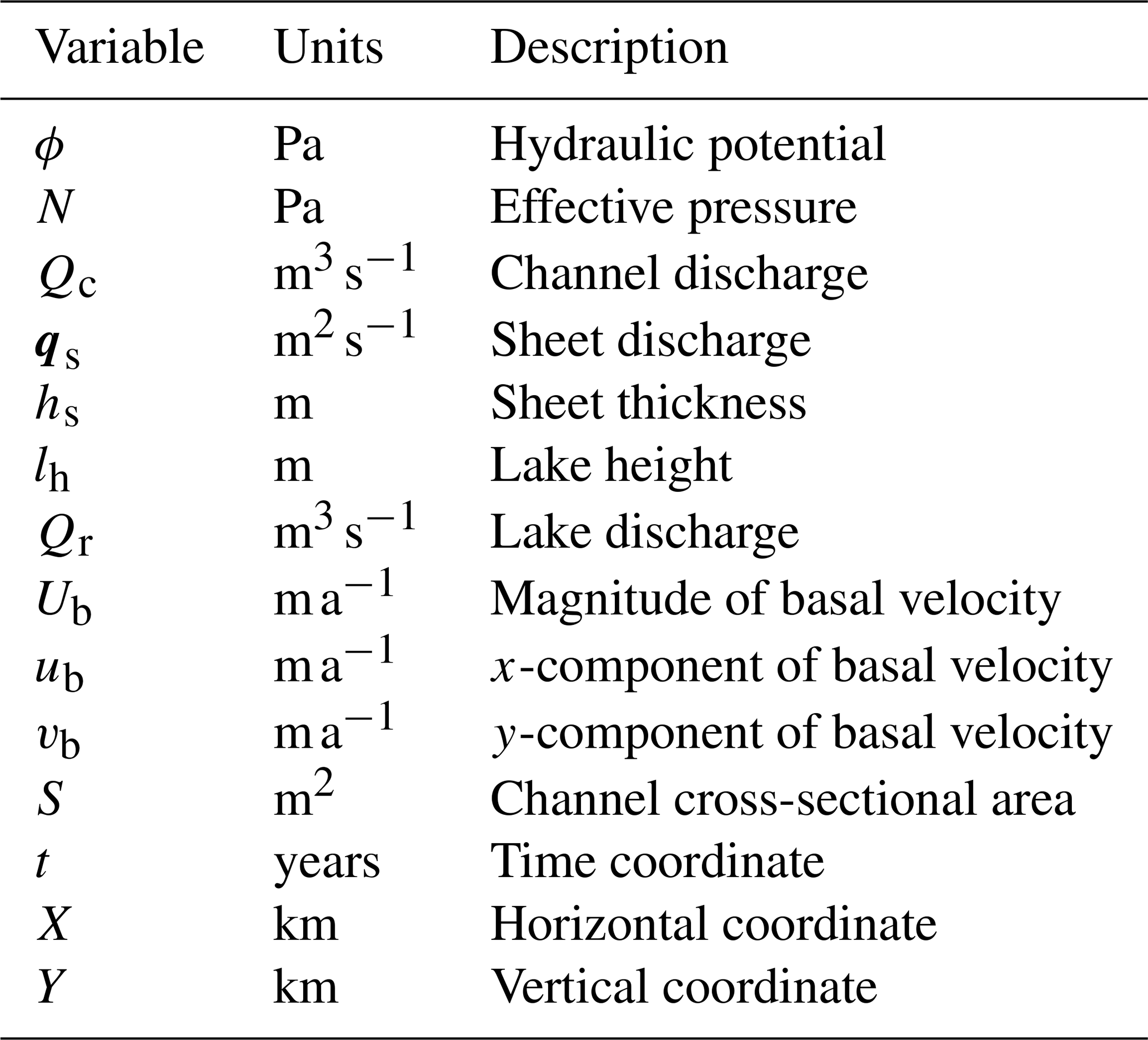
^* The first section lists dependent variables and the second section lists coordinates.

Appendix C: Additional sensitivity tests

Figure C1 Lake water height, l_h (left panel, a) and sum discharge at the ice–lake contact, Q_r (right panel, b) for the englacial void ratio e_v parameter in our synthetic experiments. In each panel, the reference parameter experiment (Sect. 3) is shown in grey.