Reduced surface hoar in a warming world

Surface hoar formation is a critical snow metamorphism process that influences the surface roughness, radar-scattering properties, albedo, and avalanche risk of snowpacks. Despite its importance, surface hoar mechanisms and climate sensitivity remain poorly constrained, creating uncertainties in remote sensing of snow properties and infrastructure hazard forecasting. To address these gaps, we use observations from the Surface Atmosphere Integrated Field Lab (SAIL) alongside the Structure for Understanding Multiple Modeling Alternatives (SUMMA) physics-based model to investigate contemporary and future surface hoar dynamics in a representative mid-latitude snow environment in the Colorado Rockies. Modeling and observations are centered around seven high-quality manual measurements of surface hoar mass during February 2023. We confirm that surface hoar is favored on clear nights with snow surfaces that are ∼ 10 °C colder than the near-surface air, leading to a favorable humidity gradient for water vapor deposition from the atmosphere onto the snowpack. Nocturnal clouds exert a 30–40 W m⁻² radiative forcing that inhibits the snowpack from cooling, thereby limiting deposition. We evaluate stability correction parameterizations and surface roughness parameters for the SUMMA model using co-located vertical gradients and eddy-covariance observed fluxes, finding that models must use an appropriate stability correction for the highly stable surface layers characteristic of surface hoar (bulk Richardson number >0.2) to model deposition rates sufficient to explain observed surface hoar mass. After taking these factors into account, both SUMMA and observations agree that deposition fluxes are favored when overnight air temperatures are less than −8 to −10 °C and horizontal wind speed is less than 2 to 3 m s⁻¹. Sensitivity experiments demonstrate that surface hoar is favored for low-density snowpacks via a thermal conduction mechanism. Using SUMMA forced by an ensemble of 9 downscaled GCMs shows that, at the annual timescale, the total wintertime nocturnal water vapor flux onto the snowpack decreases in magnitude at a rate of 6.1 gm⁻² per degree of warming, yielding an 81 % decrease by the end-of-century under the SSP3-7.0 emission scenario. This decline is driven by a 14 % decrease in nightly surface hoar events per winter and an overall increase in the size and frequency of nocturnal sublimation events. Additional work reconciling observed and modeled amounts of surface hoar mass, turbulent exchanges of water vapor during high stability, and relationships to katabatic winds in complex terrain is warranted in order to improve the understanding of this fundamental snow metamorphosis process.

1 Introduction

Surface hoar (or hoar frost) are ice crystals that grow on snow surfaces under clear nighttime skies (Colbeck, 1988; Stössel et al., 2010; Feick et al., 2007) that may persist in the snowpack for multiple days (Lang et al., 1984). Like other snow metamorphism processes, surface hoar may impact albedo (Warren, 1982; Horton and Jamieson, 2017), surface roughness and turbulent exchange (Andreas, 2002), emissivity (Hori et al., 2006), radar-scattering properties of the snowpack (Snehmani et al., 2015; Shi and Dozier, 1995), and the specific surface area of the snowpack (Libois et al., 2015). If buried by subsequent snowfall, surface hoar can create weak layers that act as initiation points for slab avalanches, which are the most destructive category (Jamieson and Schweizer, 2000; Schweizer et al., 2003; Bergfeld et al., 2023; Mayer et al., 2024). Birkeland (1998) found that 31 % of avalanches reported in Montana during the mid-1990s were associated with buried surface hoar layers.

Observations and climate projections point towards drastic ongoing and anticipated cryospheric changes in bulk snow properties such as snow-covered area and snow water equivalent (Notarnicola, 2020; Siirila-Woodburn et al., 2021). However, changes in snow microstructure are more difficult to quantify (Beniston et al., 2018), with implications for understanding avalanche hazards and associated economic impacts (Eckert et al., 2024). Some uncertainty arises due to scale mismatches between macroscale climate trends and microscale phenomenon responsible for snow grain metamorphosis, including surface hoar. For instance, even high resolution climate models use simplified representations of snow with a limited number of model-layers (Cristea et al., 2022), complicating their use for interpreting microscale exchanges such as surface hoar.

Multiple pathways may result in near-surface ice crystal growth phenomena (Style and Worster, 2009), but it is generally accepted that surface hoar forms by atmospheric water vapor deposition (Hachikubo and Akitaya, 1997) – the opposite mechanism of sublimation (Sexstone et al., 2018; Lundquist et al., 2024; Schwat et al., 2025). Molecular diffusion alone of atmospheric water vapor through the viscous sublayer onto snow grains is too slow to explain surface hoar accumulation, so turbulent exchange is necessary (Colbeck, 1988). The significance of turbulence exchange for surface hoar growth/inhibition is well recognized (Colbeck, 1988; Hachikubo and Akitaya, 1997; Föhn, 2001; Feick et al., 2007; Stössel et al., 2010; Slaughter et al., 2011), but reveals a paradox – turbulent exchange is required for surface hoar to form, but all qualitative observations suggest that windy (i.e., turbulent) nights typically preclude surface hoar formation. Explanations to resolve this paradox differ. Hachikubo and Akitaya (1997) postulates an ideal threshold wind speed (1–2 m s⁻¹) for surface hoar growth, above which sensible heat flux warms the snow, limiting the snow-to-atmosphere temperature and humidity gradient. In this vein, Colbeck (1988) suggested that light katabatic winds interspersed with unsteady bursts of turbulence provide the ideal mixing necessary for surface hoar formation. Alternatively, Feick et al. (2007) proposed the opposite, stating that katabatic winds “dry out the air” and inhibit surface hoar formation.

The tension in the literature underscores the limited understanding of surface hoar formation mechanisms, and consequently constraints on the climate sensitivity of this fundamental snow metamorphism process. To confront these questions, we use data from the Surface Atmosphere Integrated Field Laboratory (SAIL; Feldman et al., 2023), Study of Precipitation, the Lower Atmosphere and Surface for Hydrometeorology (SPLASH; de Boer et al., 2023), and Sublimation of Snow (SOS; Lundquist et al., 2024) field campaigns, located in the East River Watershed (ERW) near Crested Butte, Colorado. Together, the “S3” field campaigns collected simultaneous observations of the atmospheric energy budget (Rudisill et al., 2025; Sedlar et al., 2024; Adler et al., 2023), snow thermodynamic state, wind circulations, turbulent characteristics of the surface layer, and manual observations of surface hoar (Lundquist et al., 2024) during the winter of 2022 and 2023. Together, these observations enable a detailed analysis of the conditions that lead to surface hoar development in a representative, mid-latitude high elevation snowpack.

The goals of the study are twofold – (1) to critically evaluate the canonical model of surface hoar formation by interrogating the surface energy balance, humidity gradients, antecedent snow conditions, and turbulence in the surface layer for a representative mid-latitude continental snow climate (2) use these insights to estimate the climate sensitivity of, and projected changes in, surface hoar formation using the physics-based Structure for Unifying Multiple Modeling Alternatives (SUMMA) hydrology and snow model (Clark et al., 2015) forced with hourly downscaled climate projection data from the WUS-D3 dataset under the SSP3-7.0 scenario (Rahimi et al., 2023).

The paper is structured as follows. Section 2.1 overviews the relevant equations and theory that describe the snow energy balance and surface hoar formation process, Sect. 2.3 describes the observational data used in this study, and Sect. 2.4 describes modeling experiments and forcing data. Then, Sect. 3.1–3.3.2 investigate S3 measurements collected during the winter of 2023 and are used to inform turbulent exchange parameterization selection for SUMMA. Section 3.4 verifies SUMMA output against observations. Section 3.5 evaluates the climate sensitivity of surface hoar using SUMMA forced by the downscaled GCMs. The insights from this study will improve capacities to model and forecast surface hoar, with direct implications for avalanche hazard mitigation, the potential to improve radar retrievals of snowpack properties (e.g., Meloche et al., 2025), and snow albedo parameterizations (Flanner and Zender, 2006) in-so far as modeling this fundamental snow metamorphism mechanism is improved.

2 Methods

2.1 Governing equations

Understanding the mechanisms responsible for surface hoar formation necessitates considering both the energy and mass budgets of the snow surface, which are coupled through the latent heat flux. The following sections provide the relevant physical background for describing these relationships. Symbols and acronyms mentioned in this paper are summarized in Appendix A1 and A2.

2.1.1 The Snow surface energy balance

Using meteorological sign conventions for turbulent fluxes, the energy budget of a non-melting snow surface (_sfc) of height (h) under non-precipitating conditions with volumetric ice-fraction v_i is given by:

$$\begin{array}{}\text{(1)}& {\displaystyle }\begin{array}{rl}& \underset{\text{Snow Temp. Change}}{\underbrace{{\mathit{\rho }}_{\mathrm{i}}{v}_{\mathrm{i}}h\cdot c_p^{\mathrm{i}}{\displaystyle \frac{\partial T_{\mathrm{sfc}}}{\partial t}}}}=\underset{\text{Conduction}}{\underbrace{-\mathit{\lambda }{\displaystyle \frac{\partial T}{\partial z}}{|}_{z=h}}}\underset{\text{Turbulent Fluxes}}{\underbrace{-H_{\mathrm{s}}-H_{\mathrm{l}}}}\\ & +\underset{\text{Radiation}}{\underbrace{\mathrm{LW}\downarrow -\mathit{ϵ}\mathit{\sigma }{T}_{\mathrm{sfc}}^{\mathrm{4}}+\mathrm{SW}\downarrow (\mathrm{1}-\mathit{\alpha })}}\end{array}\end{array}$$

where $c_p^{\mathrm{i}}$ is the specific heat capacity of ice, T_sfc is the temperature of the topmost snow layer of height h, ρ_i is the density of ice, $\mathit{\lambda }\frac{\partial T}{\partial z}$ is the conductive heat flux from/out of the top snow layer to lower layers (z is positive upward from the snow ground interface), λ is thermal conductivity of the snow layer interface, H_s is the sensible heat flux, H_l is the latent heat flux, LW↓ is the incoming longwave radiation from the atmosphere (3.5–50 µm), $\mathit{ϵ}\mathit{\sigma }{T}_{\mathrm{sfc}}^{\mathrm{4}}$ is the outgoing longwave emission (LW↑) from the snow surface where ϵ is emissivity and σ is the Stefan-Boltzmann constant ($\mathrm{5.67}\times {\mathrm{10}}^{-\mathrm{8}}$ W m⁻² K⁻⁴), $\mathrm{SW}\downarrow (\mathrm{1}-\mathit{\alpha })$ is the net absorbed shortwave (solar) radiation where α is the snow surface albedo (Lundquist et al., 2024). For non-melting conditions, H_l is the energy associated with vapor sublimating (+H_l) or depositing (−H_l) onto the snowpack. At nighttime and in the absence of precipitation, H_l is balanced by H_s, the LW_net budget, cooling of the uppermost snow layer ($c_p^{\mathrm{ss}}\frac{\partial T_{\mathrm{sfc}}}{\partial t}$), and the conduction of heat into/out of lower layers of the snowpack ($-\mathit{\lambda }\frac{\partial T}{\partial z}$). From the perspective of observing LW↑ emitted by the snowpack, the depth h for which Eq. (1) is defined is small since LW↑ is primarily emitted from the snow crystals very near the surface of the snow (Morstad et al., 2007).

2.1.2 Turbulent fluxes

According to most prevailing theories, surface hoar forms via the deposition of water vapor from the atmosphere onto the snow surface (Hachikubo and Akitaya, 1997; Stössel et al., 2010). The sensible, latent, and momentum fluxes between the snow surface and atmosphere (Lee, 2023) are given by:

$$\begin{array}{}\text{(2)}& {\displaystyle }{l}_{\mathrm{s}}^{-\mathrm{1}}{H}_{\mathrm{l}}=\mathit{\rho }\stackrel{\mathrm{‾}}{w^{\prime }{q}^{\prime }}=\mathit{\rho }{C}_{q}u\mathrm{\Delta }q\text{(3)}& {\displaystyle }{c}_p^{-\mathrm{1}}{H}_{\mathrm{s}}=\mathit{\rho }\stackrel{\mathrm{‾}}{w^{\prime }{T}^{\prime }}=\mathit{\rho }{C}_{\mathrm{h}}u\mathrm{\Delta }T\text{(4)}& {\displaystyle }\mathit{\tau }{\mathit{\rho }}^{-\mathrm{1}}=u_{\star }^{\mathrm{2}}=C_d{u}^{\mathrm{2}}\end{array}$$

where the rightmost term represents the bulk approximation for the flux (Armstrong and Brun, 2008; Andreas, 2002), Δq and ΔT are stand-ins for the air-snow specific humidity (q) and temperature differences (q_sfc−q_air and T_sfc−T_air), w^′ is the deviation from the mean vertical wind velocity, u is the horizontal wind speed (w_spd) at the height z, C_q and C_h are the bulk transfer coefficients terms for q and T respectively, C_d is the bulk transfer coefficient for momentum, ρ is the air density, and τρ⁻¹ is the surface shear stress. l_s and c_p are the latent heat of sublimation (2838 kJ kg⁻¹) and specific heat capacity of dry air (1.006 kJ kg⁻¹ K) which are treated as constants. The small temperature dependency of c_p is not considered in this study. Since we are ultimately concerned with surface hoar mass, we let $F_q=l_{\mathrm{s}}^{-\mathrm{1}}{H}_{\mathrm{l}}$ as a stand-in for the left hand term of Eq. (2), which expresses water vapor flux (units of mass per unit area per time). While not a primary focus of the paper, the friction velocity u_⋆ is important for understanding turbulent exchange during surface hoar events.

Most land and snow models use some form of the bulk approximation to estimate fluxes (rightmost terms of Eqs. 2–4). Eddy-covariance (EC) instruments on the other hand can estimate fluxes by measuring q_air, T_air, and wind velocity components at a high temporal frequency (middle terms of Eqs. 2–4). Monin-Obukov (MO) theory is typically invoked to determine bulk transfer coefficients, which depend on both the characteristics of the surface and the thermodynamic stability of the near-surface air which can enhance (unstable) or suppress (stable) turbulent eddies through buoyancy forces (Foken, 2006). In the SUMMA model, bulk transfer coefficients for momentum, moisture, and heat are expressed as,

$$\begin{array}{}\text{(5)}& {\displaystyle }{C}_q={\displaystyle \frac{k^{\mathrm{2}}}{\left[\ln \right(z/z_{\mathrm{0}}\left)\right]\left[\ln \right(z/z_q\left)\right]}}\cdot f\left(Ri\right),\text{(6)}& {\displaystyle }{C}_{\mathrm{h}}={\displaystyle \frac{k^{\mathrm{2}}}{\left[\ln \right(z/z_{\mathrm{0}}\left)\right]\left[\ln \right(z/z_h\left)\right]}}\cdot f\left(Ri\right),\text{(7)}& {\displaystyle }{C}_d={\displaystyle \frac{k^{\mathrm{2}}}{\left[\ln \right(z/z_{\mathrm{0}}){]}^{\mathrm{2}}}}\cdot f\left(Ri\right),\end{array}$$

where z is the measurement height, z₀, z_q, and z_h are the roughness lengths for momentum, moisture, and heat respectively, k is the von-Karman constant (0.4), and f(Ri) is the stability correction function. The bulk Richardson number (Ri) is given by:

$$\begin{array}{}\text{(8)}& Ri={\displaystyle \frac{z\mathrm{9.81}(T_{\mathrm{air}}-T_{\mathrm{sfc}})}{\mathrm{0.5}(T_{\mathrm{air}}+T_{\mathrm{sfc}})u^{\mathrm{2}}}}.\end{array}$$

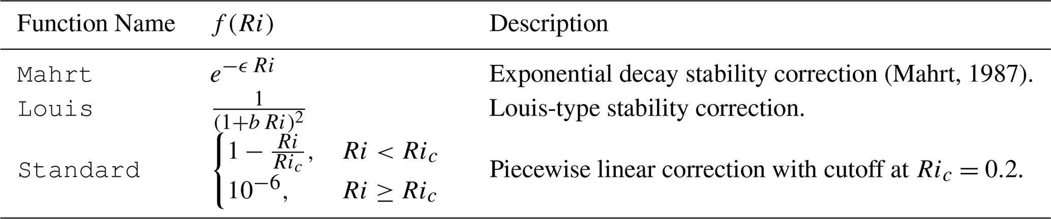
Positive Ri values indicate stable conditions and negative values indicate unstable conditions. For simplicity and in keeping with many land models, z_q, z_h, z₀ are assumed to be equivalent, but z_q may in principle be significantly less than z₀ (Andreas, 2002). Given that we are concerned with nighttime winter processes, we test several stability correction functions implemented in the SUMMA model (described in Sect. 2.4) for stable conditions (Table 1). The a, ϵ and Ri_c parameters in Table 1 are tunable coefficients. For each function, f(Ri) approaches unity at neutral conditions (Ri∼0). The Ri_c parameter in the standard model is commonly assumed to be 0.2, beyond which turbulent exchange is effectively zero.

Table 1 Stability correction formulations for stable conditions, as implemented in the SUMMA model for bulk transfer coefficients.

2.1.3 Snow surface temperature and humidity

The humidity of the snow surface (q_sfc) is saturated with respect to ice, and thus depends solely on T_sfc and P_baro. The radiative surface temperature is commonly used to represent T_sfc in Eq. (3) (Mahrt and Vickers, 2005), and can be found by rearranging the Stefan-Boltzmann law expressed in Eq. (1) (Raleigh et al., 2013).

We assume that snow emissivity (ϵ_ss) is 0.98 (Huang et al., 2016). For air and the snow surface, q is computed by:

$$\begin{array}{}\text{(9)}& q={\displaystyle \frac{\mathrm{0.622}e}{P_{\mathrm{baro}}-\mathrm{0.378}e}}\end{array}$$

where e is the vapor pressure (in hPa) and P_baro is the barometric air pressure. For snow, e is computed using the saturation vapor pressure formula for ice (Huang, 2018) using the radiative T_sfc retrieved from LW↑ measured by down-looking pyrgeometers.

2.1.4 Decomposing nightly surface hoar amounts

Together, the snow energy budget (Eq. 1), flux formula (Eq. 2), and q_sfc relationship to T_sfc provide the governing equations that explain the sign and magnitude of F_q, which is sensitive to meteorological conditions and snowpack properties. In this study, we examine instantaneous 30 min fluxes as well as nightly and yearly averages of the integrated nighttime F_q between the snow and atmosphere. The overnight amount of modeled or observed integrated water vapor flux is simply the cumulative sum multiplied by the timestep, here denoted by ΣF_q. A night with a negative ΣF_q is considered a deposition (or, surface hoar event) and a night where ΣF_q is positive is considered a sublimation event. To express the ramifications of climate change on the changing character of the overnight integrated water vapor flux, we define:

$$\begin{array}{}\text{(10)}& \stackrel{\mathrm{‾}}{F_{q,\mathrm{tot}}}={\displaystyle \frac{\mathrm{1}}{K}}\left(j\cdot \underset{\text{avg. nightly subl.}}{\underbrace{\stackrel{\mathrm{‾}}{\mathrm{\Sigma }{F}_{q+}}}}+n\cdot \underset{\text{avg. nightly depo.}}{\underbrace{\stackrel{\mathrm{‾}}{\mathrm{\Sigma }{F}_{q-}}}}\right)\end{array}$$

where F_q,tot is the annual average amount of the integrated nightly vapor flux taking into account both sublimation and deposition, K is the number of eligible winter nights per year, n is the number of winter deposition events, j is the number of winter sublimation events, and $\stackrel{\mathrm{‾}}{\mathrm{\Sigma }{F}_{q_{+/-}}}$ is the average nightly amount of all deposition and sublimation events, respectively. To account for a potentially reduced snowpack with warming, we only consider nights where snow height (Snow_h) is greater than 0.1 m. For a non-leap year when this condition is always met, there are K=121 DJFM winter nights considered in the annual averages in Eq. (10).

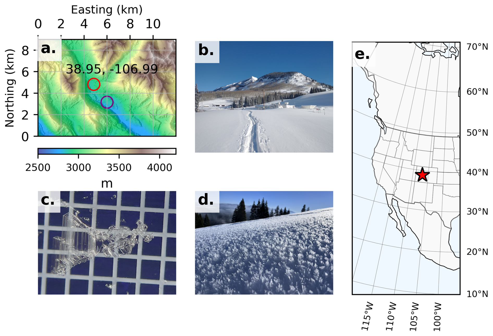
Figure 1 Overview of ERW study site: (a) A digital elevation model of the ERW with Kettle Ponds (KP) and SAIL M1 sites labeled. UTM Eastings and Northings are used for reference, and the colorbar depicts terrain elevation in m a.s.l. (b) The SAIL study site in winter, looking towards M1. (c) A surface hoar crystal observed during the SOS field campaign in the vicinity of the M1 site (photo credit: Danny Hogan, University of Washington). (d) Surface hoar crystals on a sloping snowpack, and (e) the location of the ERW in the context of the North American continent.

2.2 Study area

The ERW (38.95° N, 106.99° W) is located in the Upper Colorado River Basin and contains elevations ranging between 2440 to 4350 m a.s.l. Upper elevations of the ERW receive over 800 mm of annual precipitation, mostly as snowfall (Rudisill et al., 2023b). Overnight T_air are as low as −35 °C during winter nights (de Boer et al., 2023). Average cold-season cloud fractions are roughly 0.5 for both day and nighttime. Clear-sky periods are characterized by high pressure ridging across the western USA and upper level winds from the northwest (Rudisill et al., 2025).

Two main observing locations separated by roughly 2 km were used in this study – the main SAIL site at M1, and SOS and SPLASH sites located Kettle Ponds (KP) (Fig. 1a). Each site is located on flat terrain at the bottom of the ERW valley and contain low shrubs that are completely buried by snow mid-winter (Fig. 1b). The KP site is far away from buildings and trees and has a clear upwind fetch of at least 1 km (Lundquist et al., 2024). Figures (Fig. 1c–d) provide an example of a surface hoar crystal observed at the M1 site on 14 January 2023 and an example of surface hoar covering a hillslope, respectively.

2.3 Observations

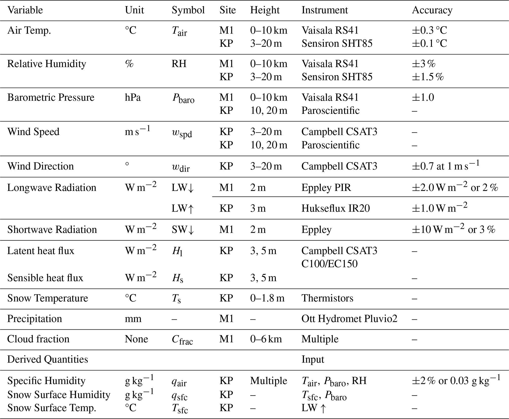
Data used in this study are described in Table 2. SAIL was a deployment of the U.S. Department of Energy's Second Atmospheric Radiation Measurement (ARM) Mobile Facility and measured of clouds, radiation, wind, and atmospheric state using both passive and active ground based remote sensing. The ARM program produces derived and best-estimate data products from the raw data streams (Mather and Voyles, 2013). Nocturnal cloud presence/absence is measured using the ARM ARSCL data product (Clothiaux et al., 2000) which merges data from a Ka-Band radar, ceilometer, micropulse lidar, microwave radiometer, and surface instruments to measure cloud properties. Cloud fraction (C_frac) is estimated temporally from this product using the same data from Rudisill et al. (2025). For visualization purposes, backscatter from the Ka-band vertically pointing radar is also shown for qualitative analysis in Sect. 2.3. Twice daily vertical profiles of atmospheric humidity and temperature were measured by balloon sondes launched at the M1 site at approximately 05:00 am and 05:00 pm local time. A weighing-bucket type precipitation gauge with a wind shield measured snowfall (Bartholomew, 2020).

The SOS campaign deployed a 20 m tower hosting measurements of T_air and RH (in addition to EC; Sect. 2.3.1) spaced at every meter of the tower. For this reason, we use meteorological variables from this site for evaluating SUMMA. Data at the lowest meter were commonly buried by snow and are not used in this study. RH is converted to q_air using T_air and P_baro (Wallace and Hobbs, 2006). The stated accuracies of the sensors yield a roughly 2 % error, or 0.03 g kg⁻¹ of q_air at representative mid-winter conditions (Table 2). SAIL pyrgeometers at M1 are used to measure LW↓ and pyranometers measured SW↓ for all analyses. Radiation data are QA/QC'd using methodologies developed by the ARM program (Long and Shi, 2006) and had a high data retention rate (Feldman et al., 2023). At the KP site, down-looking SPLASH pyrgeometers are used to retrieve T_sfc and q_sfc (Cox et al., 2025).

Near-surface meteorological data (T_air, w_spd, RH) from M1 (Table 2) is only used in one instance to examine diurnal composites of the snow energy balance (Sect. 3.2) in order to take advantage of the two-full winters of measurement (2022 and 2023), as opposed to the one winter of observations at KP (2023 only). The data platform is described in Kyrouac et al. (2021). All other uses of these variables come from KP.

Table 2 Symbol names, locations, measurement heights, and stated or estimated accuracies of observations used in this study. The accuracies from the instrument manufacturers, if available, are reported. The accuracy of KP LW↑ data are reported by Cox et al. (2025).

2.3.1 Flux measurements

In addition to low frequency measurements of T_air and RH, the SOS tower at KP hosted pairs of sonic anemometers and gas analyzers to measure EC fluxes. Data from the 3 m heights are analyzed in this study. NSF-NCAR/EOL-ISFS (2024) provides 5 min flux estimates and higher-order moments computed from the high frequency data after applying a planar fit tilt-correction (Wilczak et al., 2001). The 5 min fluxes were recomputed for a 30 min averaging timescale, and additional Webb and sonic temperature corrections were applied. EC measurements can be problematic in stable surface layers with weak turbulence, so additional tests to ensure data quality were employed (Mauder et al., 2013). Flux data were discarded if any of the gas analyzer or anemometer flags were signaled. The commonly applied stationarity tests from Foken and Wichura (1996) were also calculated. Between December and April of the SOS observation period, 62 % of the 30 min timesteps contained valid observations based on sensor flags for the sensors at 3 m, 35 % pass the least stringent stationarity criteria, and 16 % pass the most stringent stationarity criteria for heat flux. These criteria likely reject periods when overnight frost forms on the infrared hygrometers that interfere with flux measurements, but a full accounting of the prevalence of this phenomenon is beyond the scope of this article.

The measurement height between the snow and sensor is important for interpreting observed fluxes and bulk calculations. A lidar system measured the height of the snowpack in the vicinity of the towers and is used to compute the absolute height difference between the snow surface and tower measurement height. Snow_h reached a peak of approximately 2 m above the ground level (Lundquist et al., 2024).

Several considerations are important for comparing SUMMA to EC flux observations. For fair comparison against the model, EC fluxes are only considered when the second-most stringent stationarity criteria are met and the absolute value of H_s is greater than 1 W m⁻². Countergradient fluxes are also ignored, since these conditions cannot be simulated by SUMMA.

2.3.2 Stössel Box measurements

The SOS campaign manually measured surface hoar during 2023 using weighing boxes similar to Stössel et al. (2010) and Hachikubo and Akitaya (1997) referred to as “Stössel boxes” by the SOS campaign. On nine evenings in February 2023 when surface hoar was deemed likely, two snow samples were removed, weighed, and replaced in the snowpack at a location approximately a half kilometer up-valley from the M1 site. The samples were removed and reweighed the following morning. On a few occasions, a thin layer of frost was found on the underside of the box and removed prior to weighing the boxes. In the absence of disturbance, the mass difference of the snow sample between the morning and preceding evening is a measure of the cumulative deposited and/or sublimated mass of water vapor between the snow and atmosphere. Dividing the mass difference by the area of the sample yields the integrated flux (ΣF_q) in units of mass per area.

Six observations showed appreciable water vapor deposition where the redundant observations agreed within 40 %, with values ranging between 40–180 gm⁻². The morning of the 12 showed that both observations agreed on a near-zero amount of surface hoar. It is worth noting that even the largest deposition amounts represent a small component of the mass addition to the snowpack. We caution that the Stössel box measurements were not directly co-located with instrumentation at M1 or KP, but nevertheless provide confirmation that surface hoar occurred for each evening, and a plausible order-of-magnitude expectation for surface hoar mass. Thirty-three additional Stössel box measurements were collected after the end of the S3 campaigns during the winter of 2024 (Billy Barr, Rocky Mountain Biological Laboratory, personal communication). The twenty-nine measurements showed overnight deposition with an average mass of 140 gm⁻² and three measurements exceeding 200 gm⁻². Since these measurements did not overlap with S3 instrumentation, we primarily use the data as an additional check on the modelled distributions of surface hoar mass in Sect. 3.5. In addition to data from S3 campaigns, we also use data digitized from Hachikubo and Akitaya (1997) to evaluate C_q coefficients and Ri, hereafter referred to as H97.

2.4 SUMMA and downscaled GCM forcings

In addition to observations, we use the SUMMA model (Clark et al., 2015) to investigate nocturnal water vapor fluxes and the sensitivity to a changing climate. The model was configured by modifying the test-cases provided by Clark et al. (2015). SUMMA provides multiple options for modeling stability corrections for turbulent fluxes, options for simulating snow thermodynamic processes, and snow-layering schemes (Cristea et al., 2022). We use the “Jordan” snow-layering option in SUMMA that allows for up to 100 snow layers. The conduction of heat between snow layers is modelled as 1D vertical heat diffusion equation. The Jordan snow thermal conductivity parameterization was used, which treats λ as a non-linearly increasing function of snow density. Two modifications were made to the SUMMA Fortran code. The code was modified to account for the difference in q_sfc between ice and liquid water (Huang, 2018) for any situation where the ground (or snow) temperature is below freezing. The hardcoded value for ρ was also adjusted to account for elevation and average T_air. Model input files are configured so the land cover type matches that of the KP site, with no tree canopy present. Meteorological data from S3 are used to run and evaluate the model against S3 observations. SUMMA does not explicitly track the prognostic evolution of snow grain types as some snow models do (e.g., Lehning et al., 2002; Lafaysse et al., 2026) but nevertheless fits our purposes for investigating nocturnal water vapor fluxes.

To investigate SUMMA stability correction parameterizations (Table 1), we compute bulk coefficients for momentum (C_D), heat (C_h), and moisture (C_q) by rearranging Eqs. (2)–(4) using data from the SOS tower at KP. Bulk transport coefficients depend on the measurement height, so only winter data when the snow was between 0.6 and 1.2 m high is considered. Only 30 min fluxes meeting the most stringent stationarity criteria are retained for analysis (Sect. 2.3.1). Measurement errors can produce spurious results, so bin-averages are computed for intervals of Ri to highlight the underlying behavior. Only stable conditions without countergradient fluxes considered in this analysis (Lapo et al., 2019). In addition to computing C_q using EC fluxes, we also compare C_q estimates using the ΣF_q values measured by the Stössel boxes and also digitized data from H97 for comparison. To do so, we assume that surface hoar accumulated during the nighttime only and at a uniform rate.

2.4.1 Sensitivity to thermal conductivity

Examining Eq. (1) suggests that surface hoar formation may be sensitive to the thermal conductivity (λ) value and therefore the density of the snow layer, since the conductivity is strongly influenced by it (Sturm et al., 1997). To isolate the effect of snow density via thermal conductivity on surface hoar, we conduct sensitivity experiments by prescribing a constant value of λ for all layer interfaces of the snowpack representative of a low (λ=0.1), medium (λ=0.3), and high (λ=0.5) density snowpack (Sturm et al., 1997). This is achieved by using the “smnv2000” snow thermal conductivity option in SUMMA for these experiments. The model is then run for a single 36 h period encompassing a single surface hoar event and the effects on fluxes, surface energy balance, and surface hoar accumulation are quantified.

2.4.2 Sensitivity to future warming

We use data from the WUS-D3 dataset (Rahimi et al., 2023) to represent the effects of changing climate under the SSP3-7.0 emission scenario in the ERW. WUS-D3 uses the Weather Research and Forecasting model (Powers et al., 2017) to dynamically downscale (Hall et al., 2024) coarse CMIP6 (Eyring et al., 2016) model data to a 9 km horizontal grid spacing across the western United States. WUS-D3 downscaled an ensemble of CMIP6 models. We select 9 of the downscaled models to force SUMMA. Specifically these are access-cm2_r5i1p1f1, cesm2_r11i1p1f1, ec-earth3_r1i1p1f1, fgoals-g3_r1i1p1f1, ukesm1-0-ll_r2i1p1f2, canesm5_r1i1p2f1, cnrm-esm2-1_r1i1p1f2, ec-earth3-veg_r1i1p1f1m, and mpi-esm1-2-lr_r7i1p1f1 model configurations (where the text following the underscore is the model realization description).

Dynamical downscaling by WUS-D3 preserves much of the warming and wetting/drying trends from the parent GCMs (Rahimi et al., 2023) but accounts for local heterogeneity related to orography and land-atmosphere feedbacks (Walton et al., 2017). The SSP3-7.0 scenario is a moderately high radiative forcing scenario driven by “business as usual” emissions (Hausfather, 2019; Shiogama et al., 2023). WUS-D3 is extensively vetted in other snow climate studies (Cowherd et al., 2024; Marshall et al., 2024) and in addition, various configurations of the WRF model have been tested in the ERW (Xu et al., 2023; Rudisill et al., 2023a, b) demonstrating skill simulating the regional snow climate.

Hourly surface meteorological data (wind speed, downwelling shortwave radiation, downwelling longwave radiation, barometric pressure, and precipitation) from the 9 models are used to force SUMMA, yielding a total of 9 SUMMA runs from 1980 to 2100 with hourly output of surface hoar relevant quantities. Prior to doing so, two additional bias corrections to the WUS-D3 data were applied. The w_spd output from the model was bias-corrected using CDF-matching onto observed w_spd at the KP location. This method was chosen since, given the 9 km grid spacing, nocturnal drainage flows may not be well represented as the model topography is relatively coarse. In addition, a (∼1 °C) small cold bias of the average early century T_air (relative to S3) observations was found and removed. Such biases are common in dynamically downscaled output over mountain regions (Rudisill et al., 2024). Other meteorological fields were not adjusted.

In order to evaluate climate change effects on surface hoar, the ensemble of SUMMA GCM-forced experiments are evaluated using Eq. (10) for cold-season (DJFM) nocturnal conditions only, which, for simplicity are defined as between 08:00 pm to 08:00 am local time. To account for natural year-to-year variability, surface hoar relevant quantities are grouped by 20-year blocks and averaged across time. For fair comparison and to avoid including snow-free conditions into the averages, only timesteps where the Snow_h is >0.1 m are considered. Given the cold baseline climate and significant snowfall in this location, these criteria reject relatively few timesteps among the models, even at the end-of-century. To report changes, we define the beginning-of-century as 1980–2020 (BOC), the middle-of-century as 2020–2080 (MOC), and the end-of-century as 2080–2100 (EOC). In addition, data are also grouped by the average annual warming for each model year relative to the GCM's average beginning-of-century temperature (e.g., the “warming level”) in order to more clearly isolate the effects of warming from interannual variability. The statistical significance of the change in ensemble mean between the EOC and BOC periods for different surface hoar relevant variables is quantified using the Welch's two-sided t-test.

To a large extent, T_air is correlated with many other features of the snow surface energy balance (Ohmura, 2001) and rising T_air is the most basic and robust prediction for climate change. The extent to which models and observations agree with the proposed w_spd thresholds for surface hoar formation also merits consideration, and the failure by models to do so would decrease confidence in projected changes in surface hoar. Therefore, we also evaluate model and observed sensitivities for surface hoar relevant quantities to w_spd and T_air prior to evaluating the GCM-forced SUMMA experiments.

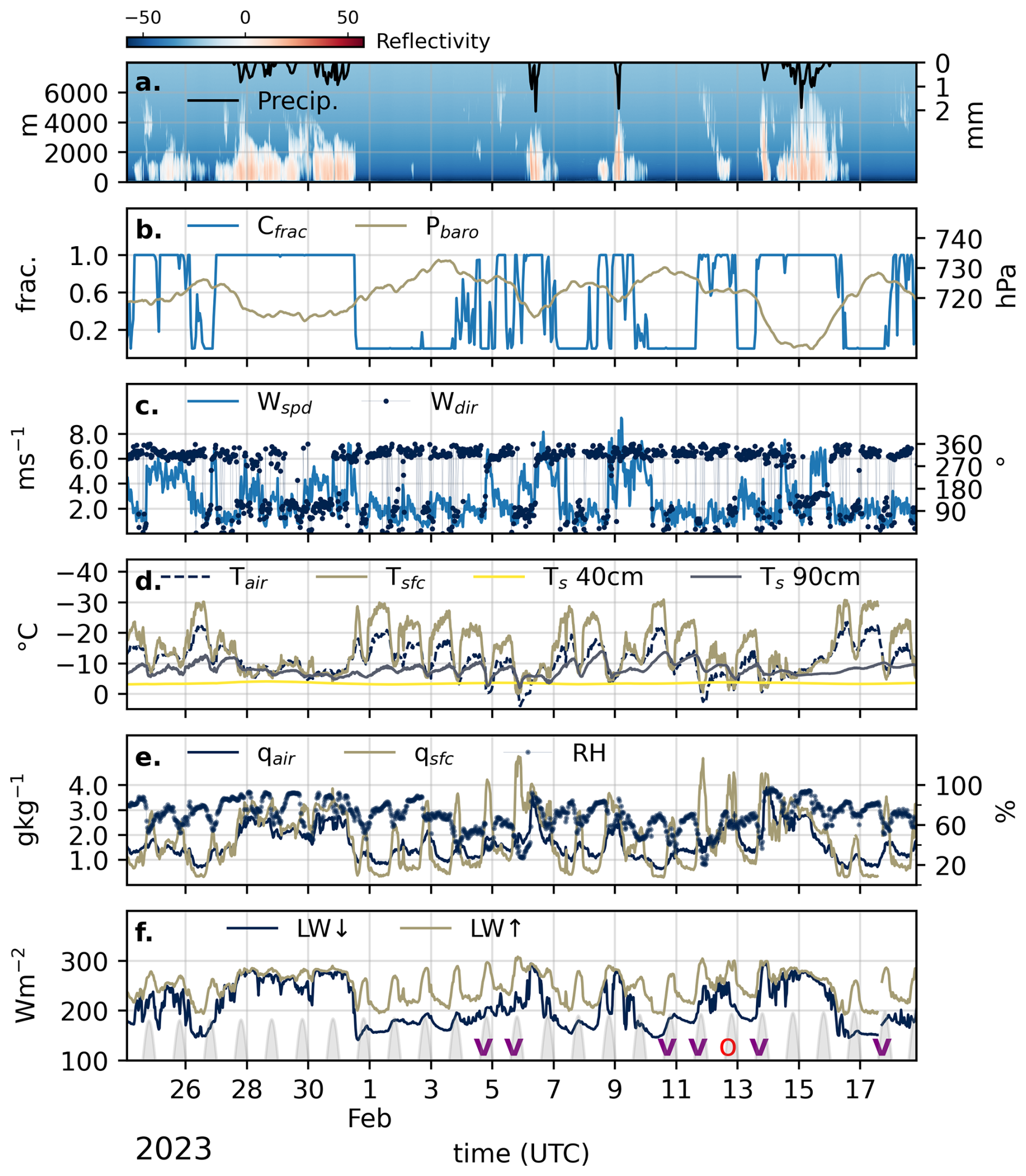
Figure 2 A time series view of the atmospheric and snowpack conditions from 25 January to 20 February 2023 during the surface hoar observation period: (a) Backscatter reflectivity from the vertically pointing Ka-band radar and hourly precipitation rates, (b) C_frac and P_baro, (c) w_spd and w_dir, (d) T_air, T_sfc, and T_snow at 40 and 90 cm above the ground level, (e) q_air, q_sfc, (f) LW↑ and LW↓. Gray shading denotes daytime periods and the solar elevation angle (the units of which are not shown). Purple V markers denote mornings when surface hoar was measured, and the red o denotes the morning of the 12 when no surface hoar was found. Please note that the y-axis of (d) is inverted.

3 Results

3.1 Atmospheric conditions during the February 2023 surface hoar observation period

To set the stage for subsequent investigation, meteorological conditions encompassing the February 2023 Stössel box observation period (Fig. 2a–f) are examined at the SOS KP site. Snow_h was approximately 1 m for the duration of this timeperiod.

Alternating periods of cloudy weather disturbances (low pressure) and clear skies (high pressure) have a clear impact on the near-surface energy budget and snowpack (Fig. 2a, b). The coldest T_air occurs on clear-sky, high pressure nights (e.g., 7–8, 16–17 February) immediately following the passage of a front when w_spd values are low (Fig. 2c, d). RH is inversely related to T_air to some degree, reaching a maximum at night, and rarely approaching saturation even during periods of snowfall (Fig. 2e). T_air is warmer than T_sfc in almost all cases, except for clear-sky periods near solar noon when T_sfc is briefly warmer than the air. However, since the snow surface is by definition 100 % RH (and atmospheric RH may be as low as 20 %), q_sfc exceeds q_air during daytime hours (favoring sublimation), but reverses on clear nights (q_sfc<q_air), favoring water vapor deposition onto the snowpack (Fig. 2e).

The snow surface is continuously cooling via LW_net on both clear days and nights (the outgoing LW↑ exceeds the incoming LW↓) (Fig. 2f). During periods with sufficiently thick clouds, however, LW_net is close to zero and there is no R_net driven cooling of the snow surface (e.g., 27–31 January). This effect occurs, in part, because clouds radiate as a gray-body with an emissivity approaching unity.

T_sfc is significantly colder than the snowpack temperature (T_snow) measured at 90 cm height (approximately 10 cm below the snow surface) for most clear-sky conditions, favoring thermal conduction of heat from within the snowpack towards the snow surface (Eq. 1). T_snow at 40 cm height remains nearly constant at −4 to −5 °C. T_sfc is warmer than the lower levels of the snowpack in only a few limited cases (e.g., the afternoon of 5 February).

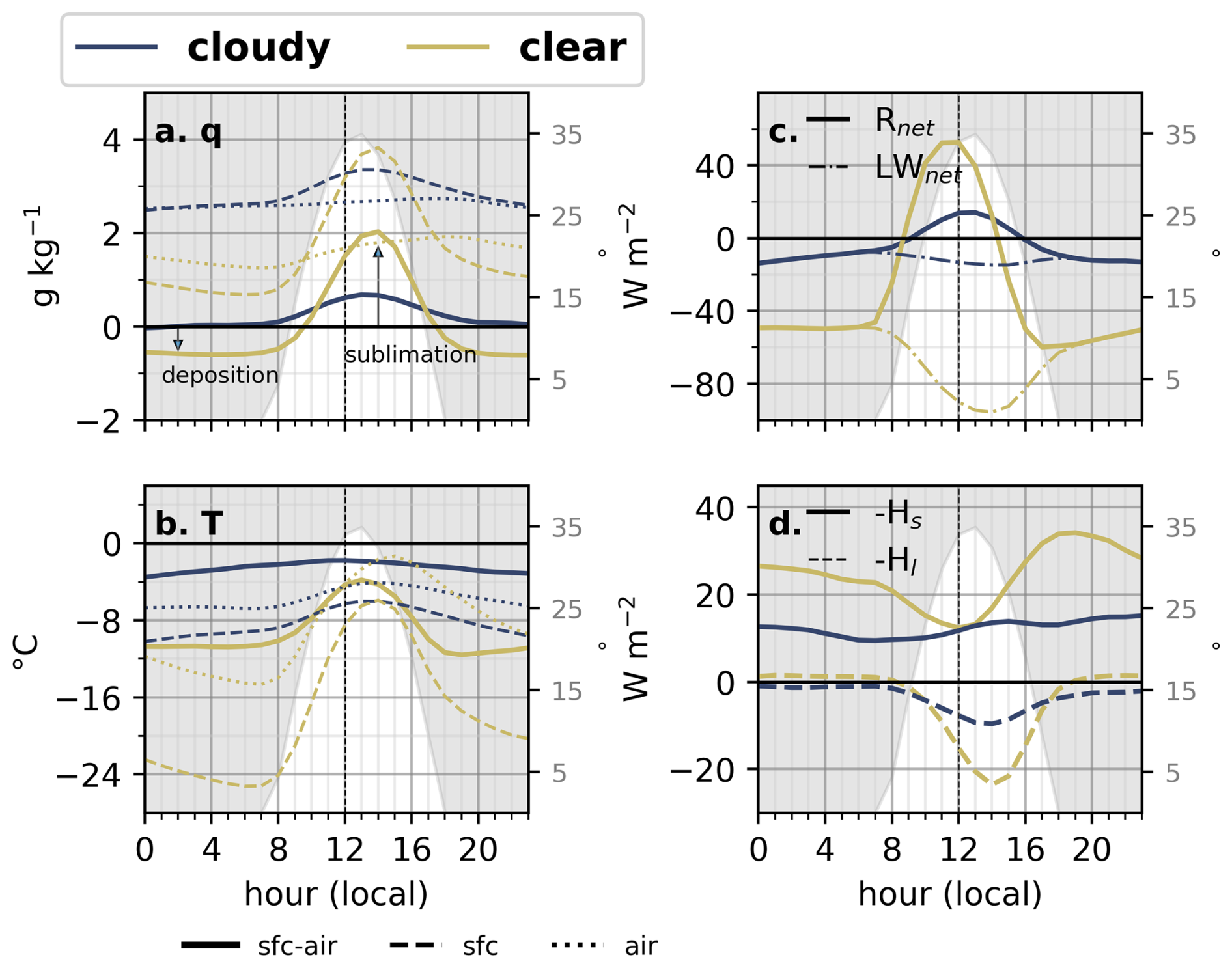
Figure 3 Composites of the diurnal evolution of observed (a) q, (b) T, (c) R_net and LW_net, and (d) turbulent fluxes (H_s, H_l) estimated from the bulk method under cloudy (dark blue) and clear (dark yellow) conditions from two winters at the M1 site. The additive inverse of H_l and H_s are depicted for convenience; positive values indicate the snowpack gains heat, and negative values the opposite. In panels (a) and (b), the dashed, dotted, and solid lines denote the snow surface, atmospheric, and snow-atmosphere difference (Δ) for T and q respectively. The vertical dashed line marks local noon and the solar elevation angle is depicted by the unfilled white region.

3.2 Diurnal cycles of humidity, temperature and energy in the snow-air interface

Building off of Sect. 3.1, the impacts of C_frac on the average diurnal cycles of humidity, temperature, R_net, and turbulent fluxes are quantified by isolating fully clear and fully cloudy 24 h periods using a temporal C_frac threshold of 0.25 and 0.95 respectively (i.e., vertically pointing cloud detections found that <25 % or >95 % of timesteps recorded a cloud within each 24 h period). For this analysis, we use two winters of data from the SAIL M1 site encompassing fully snow-covered periods from December through the end of March for each year, yielding n=61 periods meeting the clear-sky criteria and n=70 meeting the fully cloudy criteria. Fluxes are estimated using the bulk method as implemented in the SUMMA model (described in subsequent sections) with observed Δq and ΔT as inputs.

Δq is relatively constant during cloudy periods compared to clear-sky conditions (Fig. 3a). During clear-sky periods, however, overnight T_sfc and T_air drop rapidly overnight, with T_sfc reaching a minima of less than −24 °C shortly before sunrise (Fig. 3b). As a consequence, q_sfc drops rapidly on clear nights creating conditions that favor surface hoar formation (Fig. 3a). The overnight decline in T_sfc is driven, to a large extent, by negative R_net overnight with counteracting heating from turbulent fluxes. Clouds reduce LW_net cooling by 30–40 W m⁻² overnight (a measure of cloud radiative forcing consistent with Rudisill et al., 2025), acknowledging that heat-advection by snowfall may also be a component of the difference between composites.

The negative R_net is partially compensated by H_s directed towards the snow surface, which is approximately 1.5× stronger during clear-sky conditions compared to cloudy periods (Fig. 3c, d), as well as a small component of latent heating from water vapor deposition (H_l) on the order of 1–2 W m⁻² during clear-sky nights. Sublimation, on the other hand, cools the snow during the daytime for both regimes and exceeds 20 W m⁻² during clear skies just after solar noon.

The most important takeway from Fig. 3a–d is that water vapor deposition is favored, not just intermittently, but on average during clear nights (Δq values of −0.5 to −1.0 g kg⁻¹), but not on cloudy nights. Sublimation is favored during the daytime regardless of sky conditions, switching from a water vapor deposition regime to a sublimation regime around 10:00 a.m. local time (Fig. 3a, d).

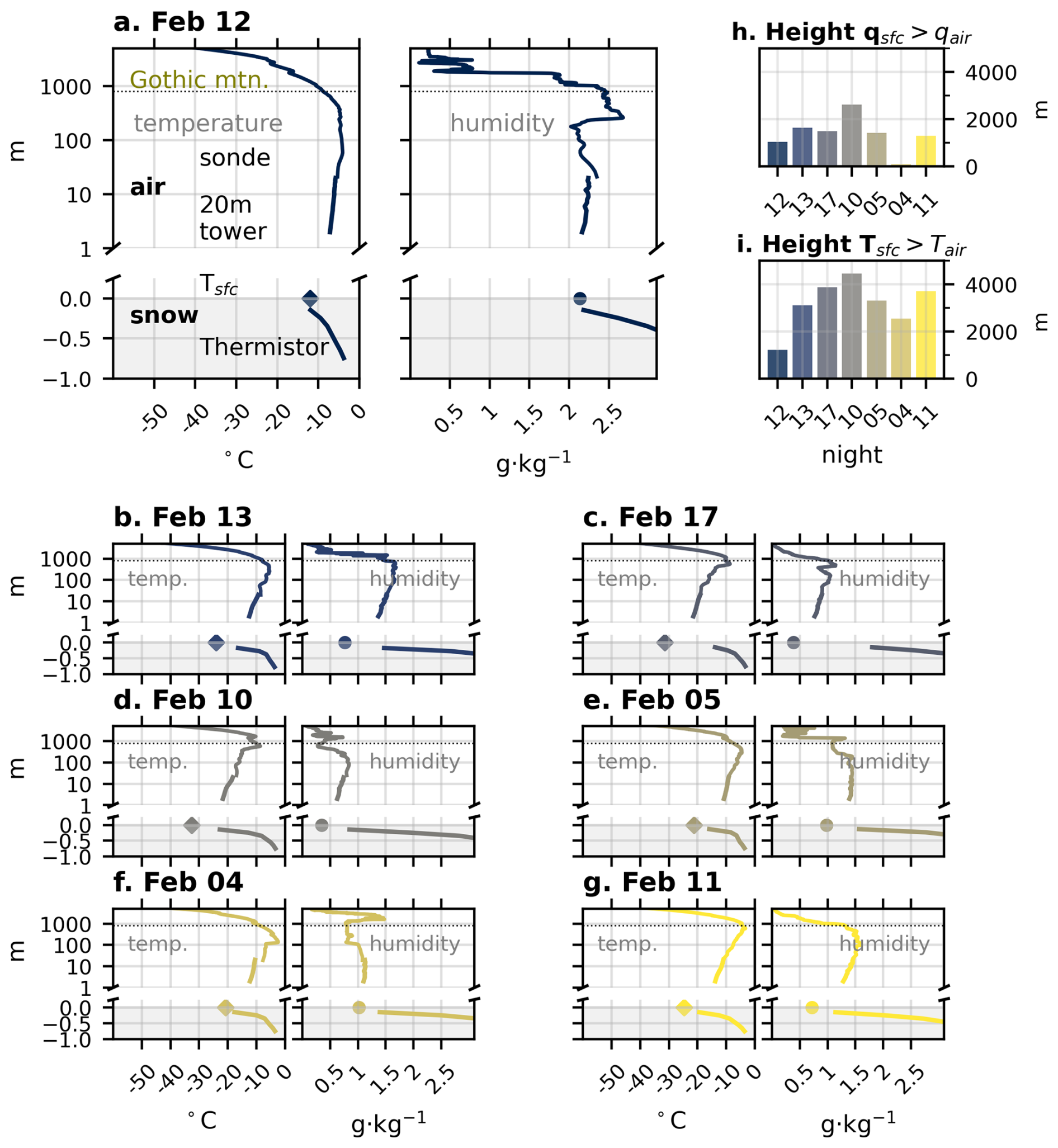
Figure 4 (a–g) 05:00 a.m. local time profiles of T_air and q_air throughout the snow-atmosphere continuum as measured by SOS towers, balloon sondes, down-looking radiometers (T_sfc), and buried snow thermistor arrays. Note the log scale y-axis. Units are heights in meters with respect to the snow surface height, defined as 0. (h, i) Barplots on the top-right depict the lowest atmospheric height level at which T_sfc and q_sfc exceeds the respective value in the atmosphere for each night. The panels are ordered by the size of the surface hoar event in the same order as (Fig. 8).

3.3 Vertical snow-through-atmosphere profiles of temperature and humidity

ΔT and Δq values are not only influenced by conditions near the snow, but also atmospheric circulations and properties of the airmass above the snowpack. To interrogate the snow-through-atmosphere continuum in the vertical direction, we examine profiles of T_air and q_air throughout the snowpack, surface layer, and troposphere using the SOS tower measurements, SAIL sondes, radiative temperature measurements, and thermistor arrays buried within the snowpack (Table 2). The balloon sondes were launched at 05:00 am local time, which is approximately the time of the T_sfc minima at this site during winter (Fig. 3b).

Figure 4a–g shows data from seven mornings coinciding with Stössel box measurements. A temperature inversion (temperature increasing with height) is present each morning when surface hoar was observed. The inversion is the weakest on the morning of the 12 when surface hoar was not observed (Fig. 2), and temperatures throughout the valley were also the warmest of those examined. In all cases, T_sfc is colder than the atmospheric temperature well above the 800 m depth of the valley (Fig. 4a, c). The nights of the 13 and 17 were significantly colder than the other observed surface hoar nights, with T_air values 100 m above the surface ranging between −15 to −10 °C (Fig. 4a). The top of the snow surface is likewise warmer than the lower levels of the snowpack, and again favor thermal conduction upwards ($-\mathit{\lambda }\frac{\mathrm{d}T}{\mathrm{d}z}$; Eq. 1) from the warm snow near the ground towards the snow surface actively cooling via LW_net at night.

The humidity of the interstitial air within the snowpack (q_snow) is estimated using T_snow as measured by buried thermistor arrays (Sturm and Benson, 1997). q_snow at the base of the snowpack near the ground surface, where T_snow approaches 0 °C, exceeds the humidity of the atmosphere at any observed level by the sondes (reaching a maximum value of >4 g kg⁻¹, which is outside the limit of the plots in (Fig. 4)). q_sfc is drier than the atmosphere well above the height of the surrounding valley. The exception is the morning of the 4, when low-level humidity leads to a scenario where the air is supersaturated with respect to q_sfc only up to 100 m above the snow surface, compared to a supersaturation height of over 2.5 km on the 10 (Fig. 4h).

These findings demonstrate that the observed negative nighttime Δq (Figs. 2, 3) are not a merely near-surface phenomenon confined to shallow heights above the snowpack, but in fact extend throughout the planetary boundary layer and well into the troposphere.

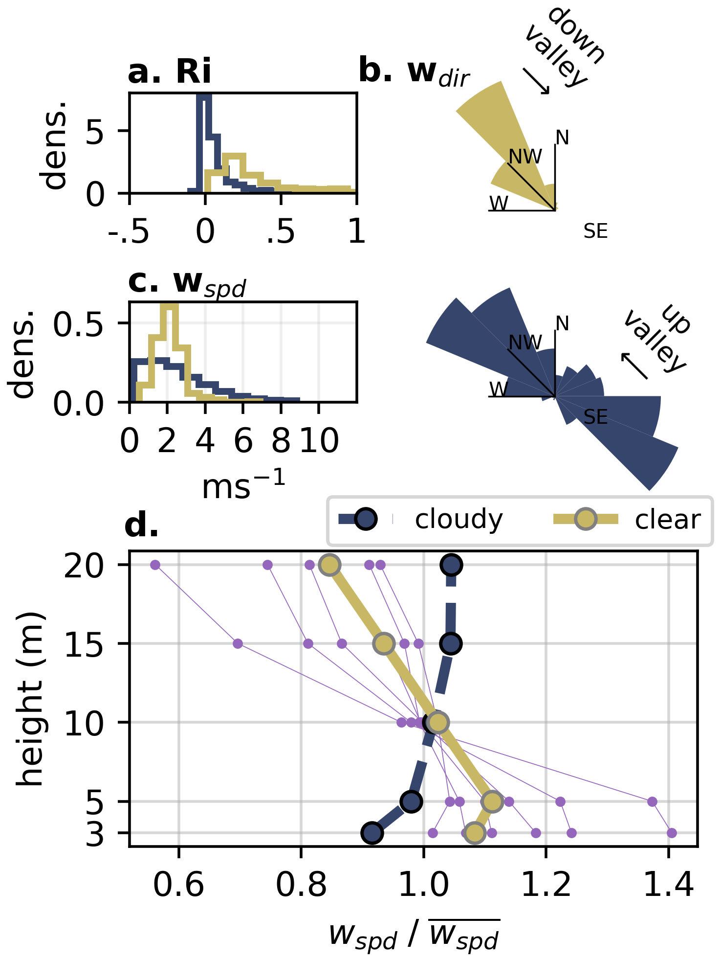
Figure 5 Wind conditions during clear and cloudy periods at the SOS KP site during winter of 2023: (a) histograms of Ri, (b) w_dir, (c) w_spd, and (d) vertical profiles of normalized wind speed ($w_{\mathrm{spd}}/\stackrel{\mathrm{‾}}{w_{\mathrm{spd}}}$). The purple lines show wind profiles for observed February surface hoar cases. Up and down-valley wind directions with respect to the valley geometry are labeled in (b).

3.3.1 Wind profiles and nighttime katabatic winds

As we have shown, favorable conditions for surface hoar tend to occur on clear, cold nights with weak synoptic forcing (Fig. 2). These conditions naturally lead to downslope katabatic flows in mountain terrain (Oldroyd et al., 2014; Whiteman, 2000; Whiteman and Barr, 1986). We already see evidence of this, given the reversal in w_dir from generally up-valley (from the southwest) during daytime hours to generally down-valley (from the northwest) at sunset (Fig. 2c; see also Adler et al., 2025).

Using the SOS tower data from the winter of 2023 and separating nights again into clear and cloudy periods shows that clear nights are typified by stronger stability as measured by Ri (Fig. 5a), w_dir almost exclusively from the down-valley direction, and shallow katabatic flows. Normalizing the vertical profile of w_spd by the tower averaged w_spd highlights the shape of the katabatic flow regime (Fig. 5d), which peaks at around 5 m above the ground level (approximately 4 m above the snow surface in the mid-winter). The strength of the jet is relatively weak, and on average is roughly 10 % higher than the mean w_spd across the entire 20 m tower. While the average maxima is found at 5 m, in many cases on clear-sky nights, the w_spd maxima is found at the lowest available measurement height. Disturbed, cloudy periods, however, have a higher average w_spd and both up and down-valley directions and a more commonly unstable or weakly stable surface layer. In these conditions, w_spd versus height follows the standard log-linear profile of increasing w_spd with height.

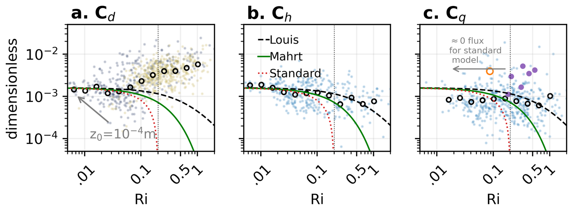
Figure 6 Relationship between Ri and the bulk transfer coefficients for (a) momentum (b) heat, and (c) moisture computed from EC fluxes and bulk gradients using Eqs. (2)–(4). Blue circles in (a)–(c) are 30 min values for all time periods considered and black open circles are bin-averages. Yellow circles in (a) denote clear-sky conditions. Purple and orange circles are estimated from Stössel box observations and digitized data from H97 respectively in (c). The solid, dashed, and dotted lines correspond to theoretical stability correction curves using the Mahrt, Louis, and standard parameterizations implemented in the SUMMA model and $z_{\mathrm{0}}=\mathrm{2}\times {\mathrm{10}}^{-\mathrm{4}}$.

3.3.2 Evaluating turbulent exchange parameterizations and surface roughness

Previous sections have investigated Δq and ΔT, but quantitative estimates of turbulent exchange require taking the buoyant suppression of turbulence and surface roughness into account. Finally, f(Ri) functions from SUMMA (Table 1) are compared against the bin-averages (Fig. 6). Generally speaking, the assumption of a $z_{\mathrm{0}}=\mathrm{2}\times {\mathrm{10}}^{-\mathrm{4}}$ m surface roughness for momentum, heat, and moisture leads to a reasonable approximation of bulk transfer coefficients. This is found by noting the intersection of the f(Ri) functions at near-neutral (Ri=0) conditions with the observed bin-averages (Fig. 6.) The effect of a higher or lower z₀ value can be visualized by recomputing (Eqs. 7–6) which has the effect of translating the f(Ri) curves up/down along the y-axis. C_q is perhaps slightly less than theoretical estimates, which is consistent with evidence suggesting that z_q≪z₀ during certain condition over ice (Andreas, 2002).

C_d deviates strongly and consistently from theoretical values at Ri greater than 0.1 (Fig. 6a). Closer examination shows that such conditions are almost always characterized by katabatic flows during clear skies. This is not surprising, given that the observed w_spd profile during such conditions does not follow the logarithmic profile required by MO theory. C_d is essentially an expression of turbulent intensity over the mean w_spd, so a higher than expected value indicates higher turbulent intensity during katabatic flows than non-katabatic flows for the same w_spd. C_D is well characterized at low Ri values and when w_spd increases approximately logarithmically with height (Fig. 5c).

A crucial finding emerges with relevance for subsequent modeling – surface hoar events occur at high Ri values (>0.2) beyond which the “standard” stability correction predicts a near-zero flux (Table 1). Recomputed data from H97 also demonstrate that surface hoar measured by their study occurred at a high Ri number of 0.1. The “Louis” stability correction with a b parameter set to one better matches observations of both C_q and C_h at high Ri values, and these parameters are used in subsequent sections (as well as in (Fig. 3)). However, it is important to note that C_q values computed using data from Stössel box and H97 data implies that, for at least five cases, C_q values are as much as 3–4× higher than the C_q implied by EC observations and model parameterizations using a z_q equivalent to z₀.

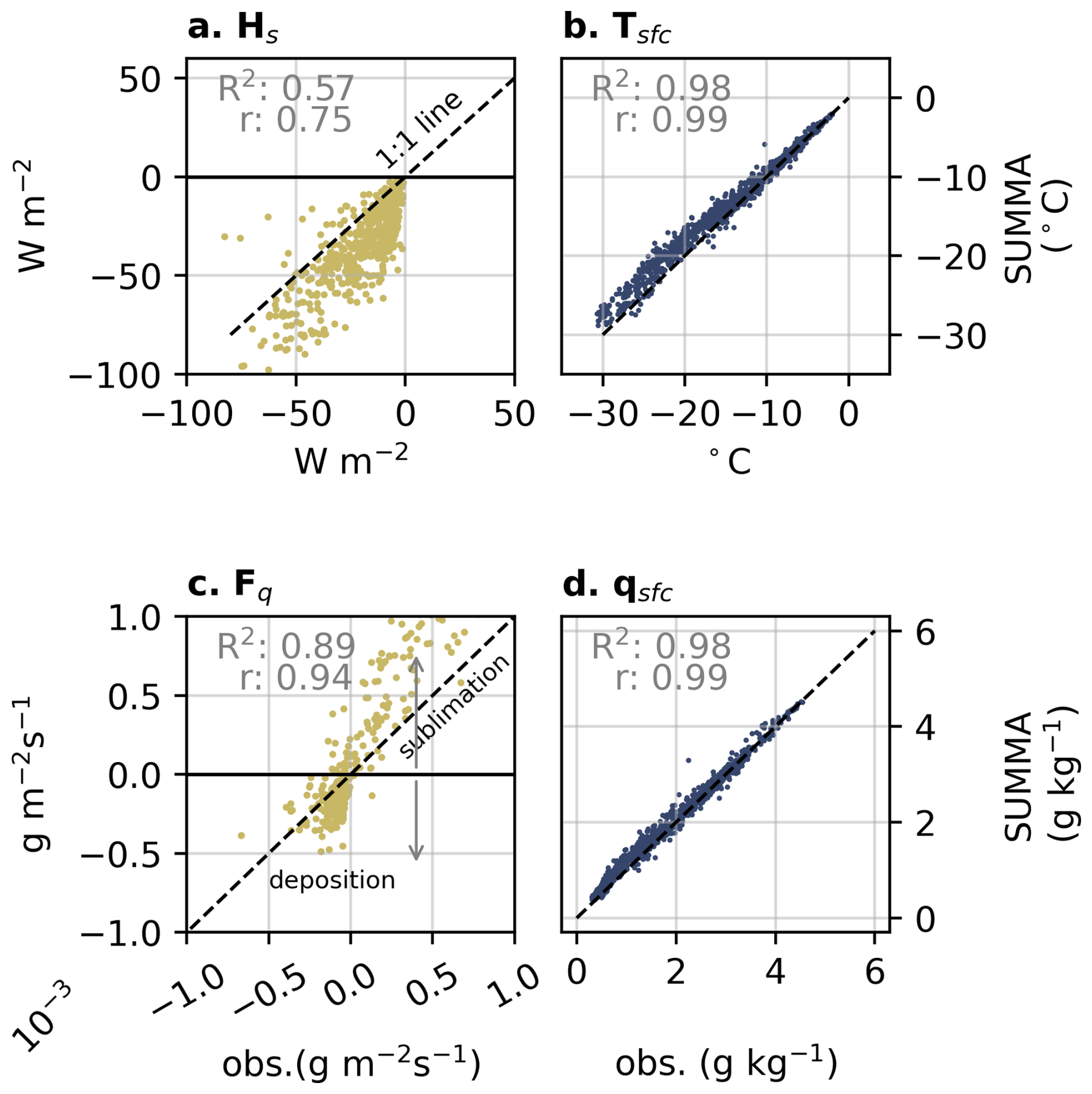
Figure 7 Comparison between observations (obs.) and SUMMA model output during winter nighttime conditions: (a) H_s, (b) T_sfc, (c) F_q, and (d) q_sfc. 1-to-1 lines (black-dashed lines) are shown for reference.

3.4 SUMMA model validation

To model the sensitivity of surface hoar to present-day and changing climates, SUMMA model parameters were selected based on data from the previous section. Prior to running the model with downscaled GCM projections (Sect. 3.5), we evaluate SUMMA using meteorological observations at S3 for winter (DJFM) nighttime conditions.

SUMMA reproduces T_sfc and q_sfc well, with Pearson correlation coefficients of 0.99 for each (Fig. 7a–d). The modeled and observed fluxes have a lower Pearson correlation coefficient of 0.75 and 0.94 for H_s and F_q respectively, and R² values of 0.57 and 0.89 (Fig. 7a, c). The model is slightly warm-biased at the coldest T_sfc values (Fig. 7b)., however these errors are somewhat mitigated when transformed to q_sfc due to the non-linear nature of the saturation vapor pressure curve (Fig. 7d). Overall the SUMMA model T_sfc is biased by 0.95 °C and q_sfc by 0.09 g kg⁻¹.

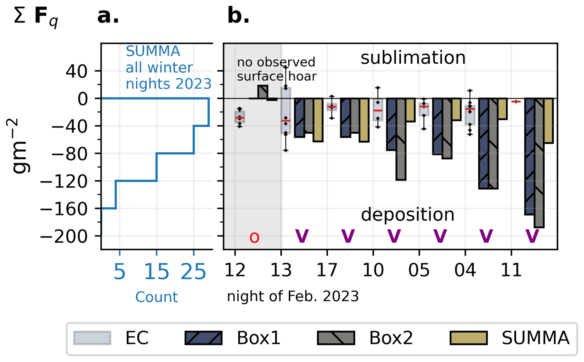
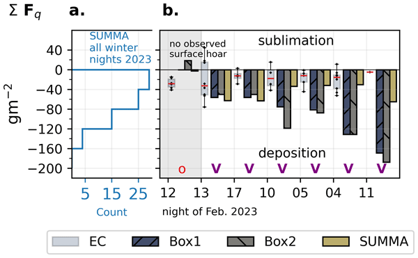
Figure 8 Validation of SUMMA against Stössel box observations: (a) histograms of total nightly cumulative deposition amount (ΣF_q) for the entire winter of 2023 from SUMMA and (b) barplots of ΣF_q for the 6 confirmed surface hoar events in February 2023 compared against duplicate Stössel box observations (Box1, Box2). Boxplots of 30 min EC fluxes observed at 3m are also depicted (multiplied by the length-of-night in seconds for purposes of comparison). The no surface hoar observation on the 12 is denoted by gray-shading in the background and the red open circle. Purple “V” markers denote nights with observed surface hoar.

Comparing SUMMA output to the deposition amounts from the Stössel box observations is a fundamentally different question than evaluating the model against 30 min EC fluxes, since ΣF_q integrates both overnight deposition and sublimation fluxes. SUMMA produces between 30–65 gm⁻² across the six events, matching the observations on the 13 and 17 well (Fig. 8a–b). However, the model produces significantly less surface hoar on the 4 and the 11 than what was observed. The largest event on the 11 was characterized by the strongest observed Δq (−0.6 g kg⁻¹) and ΔT (−12 °C) gradients, a significant amount of upper level humidity (Fig. 4), but also the highest Ri value (not shown).

Since there were relatively few high-quality fluxes observed on each surface hoar night, boxplots of the nightly 30 min fluxes are displayed in Fig. 8b. To make a fair comparison, the 30 min fluxes are multiplied by the length-of-night (assumed to be 12 h) which expresses how much water vapor could have been deposited or sublimated were the flux consistently that amount throughout the entire night. Even still, in none of the cases do the observed EC fluxes produce adequate amounts of water vapor deposition compared to Stössel box observations. This is in keeping with the observation that C_q computed from EC data in (Fig. 6) is lower than the C_q estimated by Stössel box observations. However, the median flux is negative in most cases, which does indicate that water vapor was moving in the direction of the snowpack.

No surface hoar was found on the morning of the 12. That night had moderate scattered C_frac (Fig. 2a), the lowest w_spd (Fig. 2c), high stability (not shown), and the weakest Δq (Fig. 2e) compared to the other nights with observed surface hoar. Encouragingly, the SUMMA model likewise predicted zero-surface hoar on this night.

Given all of the uncertainties in the Stössel box, EC observed fluxes, and limited temporal duration of observations, we nonetheless conclude that SUMMA is well configured for the purposes of interrogating the sensitivity of surface hoar formation to a warming climate. Additional Stössel box measurements collected up-valley from M1 during the winter of 2024 had an average mass of 140 gm⁻², which is higher than all but one of the measurements from February 2023, suggesting that spatial variability within the watershed may be significant. While SUMMA predicted less surface hoar mass for the handful of manually collected, observations, examining histograms from the entire winter shows at least 5 nights where SUMMA predicted between 120–160 gm⁻² of surface hoar, so typical amounts are within the range of the model's output space (Fig. 8a).

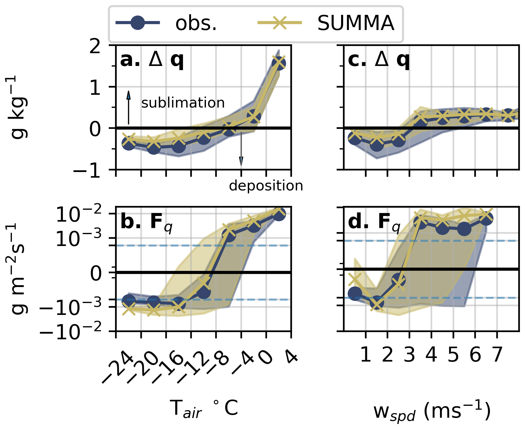
Figure 9 The sensitivity of overnight 30 min Δq and F_q to T_air (a, b) and w_spd (c, d) from both observations and SUMMA output expressed as bin-averages. Shaded regions depict the 25th and 75th percentile ranges within each bin. Note that the y-axes for (b) and (d) use a symmetric logarithmic scale, with a linear region between the blue dashed lines.

3.4.1 Observed and modelled sensitivities to T_air and w_spd

To test these sensitivities, 30 min estimates of Δq and F_q are plotted against T_air and w_spd and the same criteria for EC fluxes from the previous section are applied. Data are binned by 4 °C for T_air and 1 m s⁻¹ for w_spd, and the mean, 25th, and 75th quantile are plotted for each bin (Fig. 9a–d).

The bin-averaged Δq magnitude increases slightly beyond −24 °C but then declines rapidly (becomes closer to zero) as T_air warms (Fig. 9a). Sublimation becomes favored rather than deposition above −8 °C (Fig. 9a). Encouragingly, the SUMMA model likewise shows a transition at the same T_air. F_q shows a very similar pattern (Fig. 9b; note that the y-axis uses a symmetric logarithmic scale, with a linear region between the blue lines), though the data are noisier and have a higher inter quartile range than the model values.

The relationship with w_spd is similar (Fig. 9c, d). F_q and Δq are slightly stronger for w_spd between 1–2 m s⁻¹ compared to 0–1 m s⁻¹. Similar to other work, we find a threshold w_spd value of 2–3 m s⁻¹ that matches both observations and the SUMMA model, above which sublimation becomes favored over deposition. The bin mean of Δq at high w_spd is lesser than that at warm T_air values, indicating that w_spd alone may be a less robust predictor for discriminating water vapor deposition from sublimation than T_air.

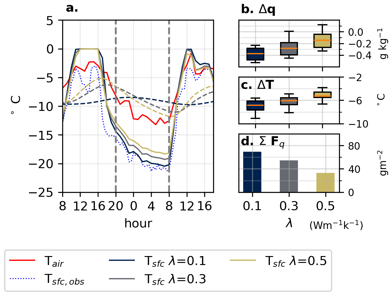
Figure 10 Sensitivity of surface hoar to prescribed values of snow thermal conductivity over a 36 h period characteristic of low (λ=0.1), medium (λ=0.3) and high-density (λ=0.5) snow: (a) Evolution of modeled T_sfc for varying λ values, with T_air (solid red line) and observed T_sfc (dotted line) included for comparison. Boxplots show (b) Δq, (c) ΔT, and (d) overnight ΣF_q (between 08:00 pm to 08:00 am, depicted by dashed gray lines in a). The line colors in (a) correspond with the bar colors in (b)–(d).

3.4.2 Modelled sensitivities to snow density vis-a-vis thermal conductivity

Ultimately T_sfc, q_sfc and overnight ΣF_q are highly sensitive to the prescribed λ value (Fig. 10a–d). During daytime hours, T_sfc reaches 0 °C for all simulations. Models diverge overnight, and the low-density simulation reaches the coldest T_sfc value (and, the most similar to the observations; (Fig. 10a)). The overnight average ΔT values are −6.5 °C for the low-density simulation compared to −5.5 °C for the high-density simulation (Fig. 10c). This translates into an average overnight Δq of −0.4 and −0.15 g kg⁻¹ respectively (Fig. 10b) Water vapor deposition occurs in all model scenarios, but a combination of the reduced deltas and stability (not shown) leads to a 54 % reduction in the overnight ΣF_q for the high-density scenario relative to the low-density scenario (Fig. 10d). The open-run model (Fig. 8) yielded an amount similar to the medium-density scenario.

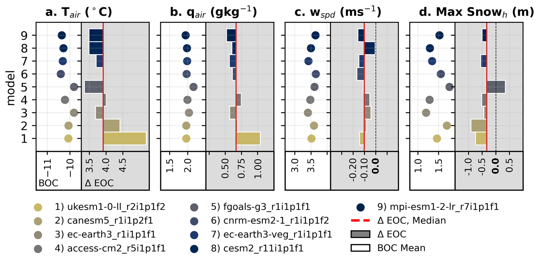
Figure 11 Effects of warming in the ERW across the 9 dowsncaled GCMs on (a) T_air, (b) q_air, (c) w_spd, and (d) maximum annual Snow_h. Left columns of each subplot depict the baseline beginning-of-century period winter nighttime average for each variable. Right columns depict the change at the EOC relative to the BOC. Red-lines depict the median change across all models for each variable.

3.5 Surface hoar in a warming climate

The intermodel average warming for the ERW across the 9 downscaled GCMs is on the order of 3.8 °C between the BOC and EOC (Fig. 11a), similar to the western USA average (Rahimi et al., 2023). q_air increases across all models the order of 0.625 g kg⁻¹ (Fig. 11b). w_spd declines slightly across most models (Fig. 11c). The annual maximum Snow_h has the greatest variability amongst the downscaled GCMs during present-day condition, but yield reasonable values of 1–2 m height for this valley location (Rudisill et al., 2023b). Maximum Snow_h decreases by 0.3 m on average at the end-of-century across all models (Fig. 11c), but increases slightly for one ensemble member.

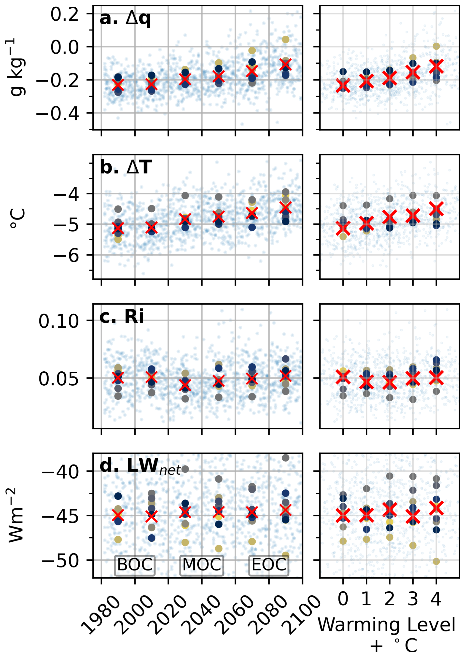
Figure 12 The change in (a) Δq, (b) ΔT, (c) Ri, and (d) LW_net, as a function of year (left column) and warming level (right column) from the SUMMA model forced by 9 downscaled GCMs under the SSP3-7.0 scenario. Blue points denote annual values and colored markers show multi-decadal means for the 9 SUMMA/WUS-D3 model runs. The colors of these values correspond with same colors in (Fig. 11). Red “×” symbols markers indicate the multi-model mean. BOC, MOC, and EOC depict the beginning-of-century, middle-of-century, and end-of-century periods.

Ultimately, both Δq and ΔT weaken (i.e., get closer to 0 °C) with warming, indicating that overnight T_sfc warms at a greater rate than that of T_air (Fig. 12a–b). There is little change in Ri, which emerges from both the competing effects of reduced thermodynamic stability (the numerator of Eq. 8) and declining w_spd (Fig. 12c). Interestingly and perhaps counterintuitively, the change in overnight LW_net remains approximately the same (within 1 W m⁻²) on average across ensembles (and the difference is not statistically significant; p>0.05), though there is significant spread and the hottest model shows a declining trend (Fig. 12d).

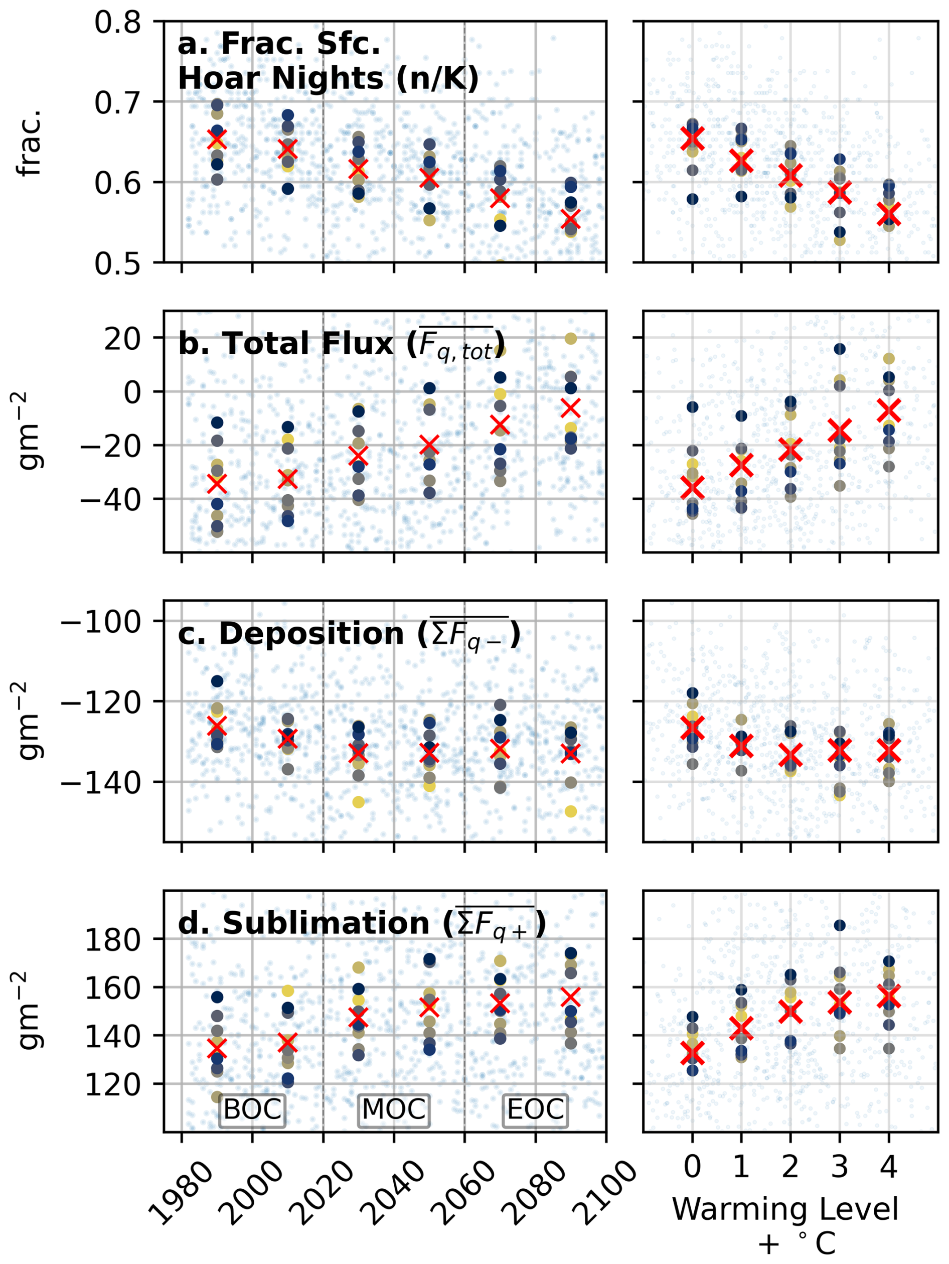
Figure 13 The same as Fig. 12, but for (a) The fraction of winter nights where the nightly cumulative ΣF_q is less than zero (i.e., surface hoar) per year, (b) the average mass of nightly total water vapor flux ($-\stackrel{\mathrm{‾}}{F_{q,\mathrm{tot}}}$), (c) the average mass of nightly deposition events ($\stackrel{\mathrm{‾}}{\mathrm{\Sigma }{F}_{q,-}}$), and (d) the average mass of nightly sublimation events ($\stackrel{\mathrm{‾}}{\mathrm{\Sigma }{F}_{q,+}}$).

3.5.1 Changes in surface hoar amount and frequency

The fraction of winter nights with surface hoar ($\frac{n}{K}$ in Eq. 10) declines linearly as a function of both time and annual warming at a rate of 2.5 nights  °C⁻¹ of warming (p<0.001, R²=0.22; Fig. 13a). The EOC experiences 14 % fewer surface hoar events per winter compared to the BOC (p<0.001). The average deposition event, $\stackrel{\mathrm{‾}}{\mathrm{\Sigma }{F}_{q-}}$, averages between 120–130 gm⁻² across all models during the BOC, remarkably similar to observations (Sect. 2.3).

$\stackrel{\mathrm{‾}}{F_{q,\mathrm{tot}.}}$ increases (becomes less negative) annually at a rate of 6.1 gm⁻² °C ⁻¹ (p<0.001, R²=0.12). Starting in the MOC and at a warming level of 3 °C, the sign of $\stackrel{\mathrm{‾}}{F_{q,\mathrm{tot}.}}$ switches for some models, indicating that sublimation contributes more to the total flux than the deposition of overnight water vapor. Averaged across all models, the annual magnitude of $\stackrel{\mathrm{‾}}{F_{q,\mathrm{tot}.}}$ decreases by 81 % by the EOC compared to the BOC (Fig. 13b) (p<0.001).

The reduction in the magnitude of $\stackrel{\mathrm{‾}}{F_{q,\mathrm{tot}.}}$ is caused by the following factors. While deposition events increase in size slightly up until 2 °C of annual warming (Fig. 13c), the frequency of those events declines. Meanwhile, the size of the average sublimation event ($\stackrel{\mathrm{‾}}{\mathrm{\Sigma }{F}_{q+}}$) increases with year and rising T_air and are 15 % larger by the EOC (Fig. 13c.) (p<0.001). At the same time, the frequency of sublimation events also increases at the complement of the decreasing rate of deposition.

4 Discussion

To our knowledge, this is the first time that 1) the full capabilities of ARM program observations, including the active remote sensing of nocturnal clouds (Fig. 2), have been used to investigate surface hoar mechanisms in a mid-latitude mountain snow environment and 2) that climate projections have been used to evaluate changes in surface hoar amount and frequency for such a region. Compared with other studies (e.g., Slaughter et al., 2011; Horton et al., 2015; Stössel et al., 2010) this work relied on comparatively few surface hoar observations but used the most detailed set of atmospheric observations to-date. We show that several existing theories of surface hoar formation are largely confirmed, but some additional important mechanisms are proposed and nuances of the relationship between climate and surface hoar are explored more than in previous work.

Colbeck (1988) suggested that katabatic winds enhance turbulence and promote water vapor exchange, and more recent work has highlighted the importance of shear-driven turbulence in the stable nocturnal surface layer in complex terrain (Sun et al., 2025). We observed stronger u_⋆ relative to w_spd (as indicated by the drag coefficient) that exceed MO-based predictions during katabatic flows (Fig. 5). The connection between turbulence during weak-wind, highly stable conditions and water vapor exchange merits additional work, as well as the roles of elevated low-level jets and other mesoscale flows impacting turbulent exchange near the snow surface (Andreas et al., 2010). The sometimes order-of-magnitude larger C_q inferred from Stössel box observations and Δq (and also found in H97 data) merits additional investigation, and may be related to the non-MO scaling of turbulence due to katabatic winds. Additional high accuracy measurements of water vapor (Harder et al., 2017) and frameworks for decomposing terms of the water vapor transport equation (Schwat et al., 2025) could potentially shed light on the role of water vapor advection during katabatic flows, which may explain the underestimates of surface hoar amount by EC fluxes as observed in this study and others (Stössel et al., 2010). In addition, it is possible that the high Ri number found at KP was not characteristic of the conditions where the Stössel box observations were taken, causing the discrepancy in ΣF_q amount between the Stössel observations and SUMMA model.

In part because of these complications, several studies using bulk methods chose to assume neutral stability and disregard stability corrections entirely (Stössel et al., 2010; Horton et al., 2014, 2015) in order to better match observations. We found, however, that choosing an appropriately long-tailed stability correction function (Mahrt, 2008) permitted reasonable amounts of surface hoar in the model, which occurs at Ri numbers (>0.2) beyond which some parameterizations cut off turbulent exchange entirely (Slater et al., 2001). In principle, near-surface Ri could change as a function of warming, though we found that Ri is balanced by both decreasing buoyant suppression (the numerator of Eq. 8) and a slight negative trends in w_spd (Fig. 11). Model fluxes are also sensitive to the chosen z₀ value (Hultstrand and Fassnacht, 2018). Our results implicitly confirmed that a value of $z_{\mathrm{0}}=\mathrm{2}\times {\mathrm{10}}^{-\mathrm{4}}$ m was reasonable for this location, but also suggest that a lower z_q value is a better fit for the data derived from EC fluxes and co-located gradients. Relatively few studies have examined the effects of unequal scalar roughness lengths for snow (Cox et al., 2025). Additional work to isolate the behavior of z_q is needed to further validate parameterizations, such as those proposed by Andreas (2002), and to test the impacts on water vapor fluxes over snow.

The fact that only low w_spd permit surface hoar accumulation (Hachikubo and Akitaya, 1997) is well characterized by both the SUMMA model and observations without the need for invoking additional mechanisms such as the mechanical destruction of surface hoar crystals by wind. The effect is described in part by climatology: strong winds greater than 2–3 m s⁻¹ are often associated with cloudy airmasses; Fig. 5 which increase H_s directed towards the snowpack, destroying the near-surface inversion and favorable Δq.

We find a more subtle interaction between q_air and surface hoar than some previous work, as the relationship between q_air and surface hoar at climatic timescales is, to some extent, the opposite from the event-scale (Feick et al., 2007). By definition, surface hoar can only form when the air immediately above the snow surface is saturated or supersaturated. However, airmasses 2–3 m above the snowpack were commonly 50 % RH–75 % RH on nights with surface hoar, whereas nights with weak Δq gradients commonly exceed 85 % RH (Fig. 2d). At the same time, the largest observed surface hoar amount was associated with the strongest Δq and the highest amounts of upper level humidity from the 05:00 am balloon sondes, so modest increases in surface hoar amount with warming may be attributable to increased atmospheric humidity. However, at climatic timescales, q_air increases across all models in tandem with T_air, yet the frequency of surface hoar declines, as well as the total amount of annually deposited water vapor. This relationship also makes sense from a geographic perspective, since at least anecdotally, surface hoar is more common in dry-continental snowpacks compared to maritime snowpacks such as those in the Sierra Nevada, and that is also more common in the cold-and-dry arctic winter than summer (Champollion et al., 2013).

The declines in surface hoar are explained by several interacting surface energy balance mechanisms (Fig. 13). Increases in q_air increase the clear-sky emissivity, yielding stronger LW↓ (in conjunction with rising T_air) following the Stefan-Boltzmann law (Brutsaert, 1975). The effect is amplified in dry-continental climates such as the ERW (Rangwala, 2013). The increase in LW↓ is compensated by an increase in T_sfc (and T_snow; not shown) such that LW_net is approximately constant with warming (Fig. 12d). As a consequence, T_sfc warms at a faster rate than atmospheric T_air, yielding a weaker Δq and ΔT (Fig. 12a, b) between the snow and atmosphere. Warmer, higher density snowpacks also have a higher λ (Sect. 3.4.2) (but a potentially weaker $\frac{\partial T}{\partial z}$, which we have not quantified) and may contribute to the warming T_sfc – in essence, lower density snow more effectively insulates the snow surface from the ground heat flux and heat gained at lower levels during daytime hours. While nocturnal water vapor deposition and sublimation are small from a water balance perspective, these fluxes represent a non-trivial component of the surface energy balance. The overnight negative R_net is balanced, in part, by H_l associated with surface hoar formation. For some perspective, an overnight 100 gm⁻² event represents 6.5 W m⁻² of heating of the snow surface (which may be as much as 15 % of the overnight clear-sky R_net; (Fig. 3)). As the snow warms, less energy is added to the snowpack via this mechanism, and the snowpack increasingly sheds energy by sublimation (Fig. 13d). Other mechanisms may also contribute to the observed declines in surface hoar. C_frac and the radiative forcing of clouds, which depend on the microphysical characteristics and atmospheric structure, are likely changing in important ways, but this analysis is left for future work (Zelinka et al., 2017).

Ultimately, many of the snow-atmosphere energy and mass exchange mechanisms leading to surface hoar formation are highly correlated with T_air itself (Ohmura, 2001; Betts et al., 2014; Arduini et al., 2019), offering lower-order proxies of surface hoar change that may be applicable to other regions. Specifically, our S3 observations found that sublimation was favored when the 30 min T_air values exceed −10 to −8 °C (Fig. 9) and w_spd exceeds 2–3 m s⁻¹. At the annual timescale scale, model results show that the annual magnitude of nightly water vapor flux $\stackrel{\mathrm{‾}}{F_{q,\mathrm{tot}.}}$ decreases at a rate of 6.1 gm⁻² per degree of warming. We postulate that warmer snowpack regions where linear warming results in a more drastic non-linear decrease in the frequency of −10 to −8 °C nights (Gottlieb and Mankin, 2024) may experience steeper declines in surface hoar compared to the cold-continental climate of the ERW. At the same time, SSP3-7.0 may represent an extreme amount of greenhouse gas radiative forcing, so the highest rates of warming presented in this study may not be realized at the end-of-century (Hausfather, 2025).

Future efforts with co-located EC instrumentation, surface energy balance data, and additional Stössel box measurements could help reduce EC, model, and manual observation uncertainties. The strong sensitivity to snow density via the thermal conduction mechanism (Fig. 10) suggests that, all else being equal, surface hoar should occur more often on clear nights following fresh low-density snowfall, though we are unaware of field observations that confirm this hypothesis. Moreover, it is commonly argued that water vapor deposition alone must be primarily responsible for surface hoar formation due to the crystal orientation, since surface hoar grows in the upward direction (Stössel et al., 2010; Fig. 1d). Yet, the strongest humidity gradients are found immediately below the snow surface on clear-sky nights rather than between the atmosphere and snow surface (Fig. 4). Additional, high vertical resolution profiles of T_snow near the surface, coincident with crystallographic observations, may shed light on the behavior of water vapor exchanges below the surface hoar layer and improve capacities for modeling this key snow metamorphosis process. Stössel et al. (2010) and Hachikubo and Akitaya (1997) note that surface hoar crystals can be maintained on the surface even when sublimation dominates the surface energy balance.

This study has focused solely on overnight water vapor exchange, which is a key step towards implementing the prognostic evolution of surface hoar layers and relevant properties in land/snow models such as SUMMA and others (Lehning et al., 2002; Lafaysse et al., 2026) for avalanche hazard forecasting, integration into remote sensing retrievals of additional snow properties such as snow water equivalent (Meloche et al., 2025), and surface albedo parameterizations. For such applications, additional work is required to relate deposited mass to relevant crystalline properties such as specific surface area. Surface hoar may increase snow albedo, serving as a counteracting mechanism to equilibrium crystal growth at the surface that tend to increase snow grain size and decrease albedo (Flanner and Zender, 2006; Armstrong and Brun, 2008). This effect was not evaluated specifically in this study, nor is such an effect included in SUMMA, but this effect may be an important consequence of declining surface hoar for the energy budget of snowpacks and rates of snowmelt and merits additional work.

5 Conclusions

Snow grains are constantly metamorphosing in response to temperature and humidity gradients – as the climate warms, changes in these processes are inevitable, with potential consequences for infrastructure, human safety, and remote sensing of snow properties. In this study, we used eddy-covariance data, surface energy balance, balloon sondes, and data from a limited number of manual surface hoar observations (Stössel boxes) to investigate overnight water vapor deposition – the process considered responsible for the majority of surface hoar formation – at a single intensively monitored site in the Colorado Rockies. Nights with surface hoar are characterized by tropospheric temperature inversions where the radiative temperature of the snow is both colder and drier (in terms of specific humidity) than the air well above the highest point of the surrounding valley (in most cases). This creates a gradient favoring atmospheric water vapor deposition onto the snow. Such conditions are favored, on average, during clear-sky winter nights, but not on nights with cloud cover, largely because clouds exert a significant overnight radiative forcing (30–40 W m⁻²) that prevents the snow surface from cooling. These same synoptic conditions lead to shallow katabatic winds with maxima very near the surface, likely generating beneficial turbulence for surface hoar formation, though more work is needed to understand the turbulent transport of water vapor in these conditions. We show that atmospheric water vapor deposition onto the snowpack can explain a significant amount of surface hoar mass, though rates observed by manual measurements and EC vary substantially in magnitude. The SUMMA model underestimated surface hoar mass in some circumstances, but nevertheless captured the magnitude and validated well against observations of the snow thermodynamic state, with biases in T_sfc and q_sfc of 0.95 °C and 0.09 g kg⁻¹.

Ultimately both observations and the SUMMA model show that humidity gradients and fluxes switch from favoring deposition to favoring sublimation when overnight T_air is warmer than −10 to −8 °C and w_spd greater than 2–3 m s⁻¹. Sensitivity experiments demonstrate that surface hoar is favored for low-density snowpacks via a thermal conduction mechanism, since low-density snow more effectively insulates the surface from heat at lower levels of the snowpack overnight. The climate sensitivity of surface hoar was quantified by forcing the model with a 9-member ensemble of bias-corrected and dynamically downscaled GCM data between 1980 to 2100. Despite increasing atmospheric humidity, the frequency of surface hoar per winter decreases by 14 % and the total amount of water vapor deposited annually onto the snowpack (taking into account both sublimation and deposition) decreases by 81 % by the EOC under the SSP3-7.0 emission scenario at a rate of 6.1 gm⁻² per degree of warming. Given the cold-continental climate of this study location, we consider these modeled declines in surface hoar as possibly low-end estimates compared to warmer snow climates.

Appendix A: List of Symbols and Abbreviations

A1 Meteorological and snowpack related variable definitions

Symbol/Acronym	Description
Tair	Near-surface air temperature
Tsfc	Snow surface (radiative) temperature
Tsnow	Snow temperature within the snowpack
Tmin	Minimum air temperature
qair	Near-surface specific humidity
qsfc	Snow surface specific humidity
	(saturation w.r.t. ice)
qsnow	Snow interstitial specific humidity
ΔT	Air-to-snow temperature difference
	(Tsfc−Tair)
Δq	Air-to-snow specific humidity difference
	(qsfc−qair)
Pbaro	Barometric pressure
wspd	Wind speed
wdir	Wind direction
Cfrac	Cloud fraction
Fq	Water vapor flux from the atmosphere
	to the snow (gm−2 s−1)
Hl	Latent heat flux (W m−2)
Hs	Sensible heat flux (W m−2)
cp	Specific heat capacity of dry air
ls	Latent heat of sublimation
Snowh	Snow height above the ground level
MO	Monin-Obukov (similarity theory)
Ri	bulk Richardson number
RH	Relative humidity
EC	Eddy-covariance

A2 Other acronyms used in this study

Symbol/Acronym	Description
SAIL	Surface Atmosphere Integrated Field
	Laboratory (field campaign)
SOS	Sublimation of Snow (field campaign)
SPLASH	Study of Precipitation, the Lower
	Atmosphere and Surface for
	Hydrometeorology (field campaign)
H97	Hachikubo and Akitaya (1997)
ARM	Atmospheric Radiation Measurement
	(program)
ERW	East River Watershed
KP	Kettle Ponds measurement site
M1	Main SAIL measurement site
S3	Collective term for the SAIL, SOS,
	and SPLASH field campaigns
SSP	Shared Socioeconomic Pathway
GCM	General Circulation Model
SUMMA	Structure for Unifying Multiple Modeling
	Alternatives (model)
WUS-D3	Western United States Dynamical
	Downscaling dataset
WRF	Weather Research and Forecasting Model
BOC	Beginning-of-century (1980–2020)
MOC	Middle-of-century
EOC	End-of-century (2080–2100)