Impact of climate forcing time step in an ice-sheet firn model

The firn layer regulates how an ice sheet responds to atmospheric climate change by modifying how changes in surface temperature, snow accumulation and ablation affect the ice-sheet mass balance. Firn properties are often simulated with a firn densification model. Prior studies have used a variety of time steps in the climate forcings of such firn models, ranging from 3 h to 1 d, 1-month, or even annual. The climate forcing time step impacts the creation of pore space by snow accumulation and the depletion of pore space by snowmelt and firn densification. To investigate this effect, we force the firn densification model IMAU-FDM with surface mass balance components and meteorological variables at different time steps for the Antarctic Peninsula and southern Greenland Ice Sheet. We show that the final modelled firn layer contains more pore space for larger forcing time steps, and that the magnitude of this effect depends on the climate regime. Locations with limited firn pore space due to seasonal melt, and regions with emerging firn aquifers, are most sensitive. The key in causing the differences in firn pore space is the presence or absence of a diurnal cycle in the input data. A climate forcing time step equal to or greater than a day allows for a non-physical coexistence of snowmelt and sub-zero surface temperatures, leading to immediate shallow refreezing of meltwater. Subsequent melting removes refrozen higher density firn rather than porous firn, reducing the amount of firn air that is lost through melting. Therefore, for locations experiencing surface melt, the decoupled temperature and snowmelt in the upper layers results in more firn air with a climate forcing time step equal to or greater than a day. We also found that model parameterizations can become unsuitable when applied outside the physical conditions or climate forcing time step on which they are based, leading to unrealistic firn densification behavior in the model. We argue that (1) firn models forced with surface mass balance terms and meteorological variables require a timestep small enough to capture at least the diurnal cycle, (2) parameterizations should be used in a way that is consistent with the development data.

1 Introduction

Firn, the transitional state between snow and glacial ice, covers ∼90 % of the Greenland Ice Sheet (GrIS) (Noël et al., 2022) and ∼99 % of the Antarctic Ice Sheet (AIS) (Winther et al., 2001). Firn contains air that prevents a fraction of the meltwater to run off into the ocean, either by refreezing or liquid water retention. Approximately ∼39 % of surface meltwater on the GrIS and ∼94 % on the AIS is retained in the firn (Medley et al., 2022). Consequently, the firn layer keeps meltwater away from crevasses, where it could otherwise enter the GrIS subglacial drainage system, or engage in hydrofracturing on Antarctic ice shelves. Also, outside the percolation zone the firn layer evolution is of relevance, as variations in firn mass and thickness complicate the interpretation of altimetry observations for ice-sheet mass balance.

Firn models are used to improve our understanding of physical processes, to interpret observations including remote sensing data, and to make projections of ice-sheet surface mass balance (SMB) in the future (The Firn Symposium Team, 2024). Firn models differ in their parameterizations and formulations for densification, thermodynamics, and water percolation processes (Vandecrux et al., 2020). Although a variety of firn models exist, all models have in common that they use numerical methods to integrate a set of coupled differential equations in time. In this paper, we focus on the fact that the upper boundary conditions for solving the equations are provided at a discrete time step. Those boundary conditions can be components of the SMB and/or surface energy balance (SEB), or meteorological variables, which varies depending on the firn model (The Firn Symposium Team, 2024). The climate forcing time step differs greatly across studies, varying from 1 h, to days, months, and even years (Sørensen et al., 2011; Simonsen et al., 2013; Langen et al., 2017; Meyer and Hewitt, 2017; Verjans et al., 2019; Stevens et al., 2020; Brils et al., 2022; Gkinis et al., 2021; Medley et al., 2022; Thompson-Munson et al., 2023; Veldhuijsen et al., 2023; Wever et al., 2023; Hansen et al., 2024; Zhang et al., 2024). Here, we focus on the climate forcing time step for the IMAU firn densification model (IMAU-FDM), which is forced with SMB and meteorological variables at the upper boundary.

Reasons for choosing a certain climate forcing time step are most often practical: the data are not available at smaller time steps, the amount of forcing data becomes too large, or the computational resources are insufficient. Evaluation of the forcing time step is often absent or based on differing lines of reasoning. For example, Medley et al. (2022) argue that the absence of a diurnal cycle in the forcing time step is a limitation of their model, whereas Meyer and Hewitt (2017) expect that the daily cycle influences only the uppermost meter of the firn column, and therefore, ignore it.

We emphasize the difference between the time step used to solve the differential equations in a model, and the time step at which the forcing data is provided. The focus of this paper is on the latter. Most often, the model time step is smaller than the forcing data time step. To clarify with an example, Veldhuijsen et al. (2023) uses a 3-hourly climate forcing linearly interpolated to a 15 min model time step.

In this paper, we demonstrate that the output of a firn model is sensitive to the forcing time step when forced with SMB and meteorological variables at the surface, while geographically focusing on the Antarctic Peninsula Ice Sheet (APIS) and the southern GrIS.

2 Methods: Firn modelling setup

We use IMAU-FDM (Brils et al., 2022; Veldhuijsen et al., 2023) to simulate the firn layer and investigate the sensitivity of the modelled firn layer to the climate forcing time step. This section describes IMAU-FDM and specifies similarities and differences in the model for the two domains. We also describe the forcing dataset, setup for testing different forcing time steps, model initialization, and study areas.

2.1 IMAU-FDM

IMAU-FDM is a 1D semi-empirical model that simulates density, temperature, and meltwater content in the firn layer. The model is originally developed by Helsen et al. (2008) and has undergone multiple updates (Ligtenberg et al., 2014; Brils et al., 2022; Veldhuijsen et al., 2023). We use IMAU-FDM v1.2A (Veldhuijsen et al., 2023) for the Antarctic domain and IMAU-FDM v1.2G (Brils et al., 2022) for the Greenland domain, which only differ from each other in their ice-sheet dependent calibration. Both versions have been evaluated extensively against firn density and temperature observations (Ligtenberg et al., 2014; Kuipers Munneke et al., 2015; Brils et al., 2022; Veldhuijsen et al., 2023).

The firn and ice column are divided into 200–3000 layers, traced in a Lagrangian framework. Snowfall is added to the topmost layer of the column, burying other layers and thereby representing downward advection. No layers are removed during a simulation. The layers have a maximum vertical resolution of 0.15 m. Layer routines are built in that split the uppermost layer if it exceeds the 0.15 m threshold and merges the two uppermost layers if the thickness of the uppermost layer is smaller than 0.05 m. When the firn column has less than 200 layers, 100 very thin layers of pure ice are added to the bottom of the column.

The fresh snow density is an upper boundary condition with different parameterizations for the AIS and GrIS domain. In IMAU-FDM v1.2A (AIS), the fresh snow density ρ₀ (kg m⁻³) depends on instantaneous surface temperature T_s (K) and 10 m wind speed ff_10 m (m s⁻¹) (Eq. 1) (Lenaerts et al., 2012; Veldhuijsen et al., 2023):

$$\begin{array}{}\text{(1)}& {\displaystyle }{\displaystyle }\mathit{\rho }{}_{\mathrm{0}}=\mathrm{82.97}+\mathrm{0.769}{T}_{\mathrm{s}}+\mathrm{11.67}{\mathit{ff}}_{\mathrm{10}\mathrm{m}}\end{array}$$

In IMAU-FDM v1.2G (GrIS), ρ₀ is based on the surface temperature averaged over the year prior to the snowfall $\stackrel{\mathrm{‾}}{T_{\mathrm{s}}}$ (K) (Eq. 2) (Fausto et al., 2018; Brils et al., 2022):

$$\begin{array}{}\text{(2)}& {\displaystyle }{\displaystyle }\mathit{\rho }{}_{\mathrm{0}}=\mathrm{362.1}+\mathrm{2.78}(\stackrel{\mathrm{‾}}{T_{\mathrm{s}}}-\mathrm{273.15})\end{array}$$

The densification of snow and the underlying firn in each layer is parameterized by a semi-empirical equation (Eq. 3) based on Arthern et al. (2010):

$$\begin{array}{}\text{(3)}& {\displaystyle }{\displaystyle \frac{\mathrm{d}\mathit{\rho }}{\mathrm{d}t}}=D\dot{b}g\text{MO}({\mathit{\rho }}_{\mathrm{i}}-\mathit{\rho }){\mathrm{e}}^{-\frac{E_{\mathrm{c}}}{RT}+\frac{E_{\mathrm{g}}}{R{T}_{\mathrm{b}}}}\end{array}$$

with $\dot{b}$ the average accumulation rate ($\mathrm{kg}{\mathrm{m}}^{-\mathrm{2}}{\mathrm{yr}}^{-\mathrm{1}}$) over the spin-up period, g the gravitational acceleration (9.81 m s⁻²), ρ_i the density of bubble-free ice (917 kg m⁻³), ρ the instantaneous layer density (kg m⁻³), E_c the activation energy for creep (60 000 J mol⁻¹), E_g the activation energy for grain growth (42 400 J mol⁻¹), R the universal gas constant (8.3145 $\mathrm{J}{\mathrm{mol}}^{-\mathrm{1}}{\mathrm{K}}^{-\mathrm{1}}$), T the instantaneous layer temperature (K), and T_b the instantaneous temperature of the bottom firn layer. D is a constant and MO is a correction term that improves model alignment with observations of the 550 and 830 kg m⁻³ density level depths (Ligtenberg et al., 2011). The correction term differs for both domains (Brils et al., 2022; Veldhuijsen et al., 2023). In this equation, ${\mathrm{e}}^{\frac{-E_{\mathrm{c}}}{RT}}$ represents the temperature-dependency of ice deformation; ${\mathrm{e}}^{\frac{E_{\mathrm{g}}}{R{T}_{\mathrm{b}}}}$ is a correction term arising from the estimated grain size (E_c>E_g). Ice grains grow faster in warmer conditions, while large grains deform slower than smaller grains, hence reducing the densification. As the current grain size is the result of the grain growth since deposition, its impact on densification must be approximated by the typical temperature conditions. Therefore, the mean firn temperature, estimated by the temperature of the lowermost layer (T_b), is used in Eq. (3).

The physical description for water percolation and heat transport is identical in both model versions. Liquid water is added to the top of the column. Its transport through the layers is calculated using the “bucket scheme”. In this scheme, each layer has an irreducible water content which is the maximum amount of water that can be retained by capillary forces. The irreducible water content decreases with increasing density (Coléou and Lesaffre, 1998). Water refreezes when in a firn layer cold content is available, reducing the pore space of the firn.

In IMAU-FDM, ice layers form through subsequent events of wetting and refreezing, whereby the density is increased and the pore space is reduced until the ice density of 917 kg m⁻³ is reached. Ice layers primarily form near the surface where sufficient meltwater and cold content allow for repeated cycles of pore space filling and refreezing. Therefore, in the current model setup, a single melt event cannot completely fill and refreeze the pore space of a firn layer. The bucket scheme does not allow standing water over ice layers. Instead, water percolates to the next layer when no pore space is available. The water percolation formulation implies that, in one model time step, water can percolate through the whole firn layer until it reaches the firn-ice interface. Any leftover water is assumed to run off.

Heat conduction through the firn layer is described by the 1D heat transfer equation, with conductivity being a function of density (Calonne et al., 2019; Brils et al., 2022). Refreezing acts as a heat source within the firn. Heat transfer at the upper boundary is governed by the prescribed surface temperature. A constant heat flux through the bottom layer is applied as the lower boundary condition.

2.2 Forcing dataset

IMAU-FDM is forced at the surface with surface temperature, 10 m wind speed, snowmelt, snowfall, sublimation, snowdrift erosion, and rainfall. These climate forcings originate from the regional atmospheric climate model RACMO2.3p2 (Noël et al., 2018; Van Wessem et al., 2018), dynamically downscaling ERA5 reanalysis data (Hersbach et al., 2020). The AIS data covers the period 1979–2023 with a horizontal resolution of 27 km×27 km and is extended from Van Wessem et al. (2018). The GrIS data spans 1 September 1939–1 December 2023 with a horizontal resolution of 5.5 km×5.5 km and is a renewed and extended version of the simulation presented by Noël et al. (2018).

2.3 Climate forcing time step

We force the model with four climate forcing time steps (dt_force) at the surface: 3 h, 6 h, 1 d and 1-month, referred to as dt_force=3 h, 6 h, 1 d, and 1 m respectively. We chose these values because (1) they are typically used to force firn models, and (2) they provide examples with and without a diurnal cycle in the input data (Fig. 1). In addition, dt_force=3 h is the smallest available climate forcing time step from RACMO2.3p2 and is commonly used to force IMAU-FDM. We averaged the 3-hourly surface mass fluxes, surface temperature, and 10 m wind speed data to get the input data for dt_force=6 h, 1 d, and 1 m. IMAU-FDM interpolates the forcing data onto a 15 min model time step in which we assume a constant value for the whole forcing period for the surface mass fluxes, surface temperature and 10 m wind speed (Fig. 1). To summarize, numerical time integration is done using a model time step of 15 min, but the climate forcing time step can be 3 h, 6 h, 1 d, or 1-month.

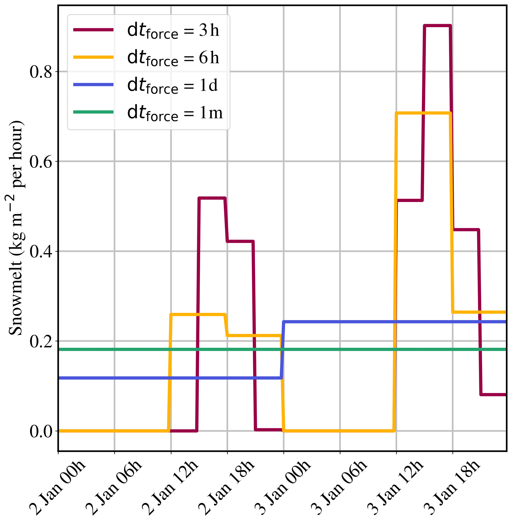
Figure 1 Example of 48 h of snowmelt forcing at dt_force=3, 6 h, 1 d, and 1 m. The graph also visualizes the model's interpolation of the forcing onto a 15 min timestep. Note the presence of a diurnal cycle in the snowmelt input for dt_force=3 and 6 h and its absence for dt_force=1 d and 1 m.

2.4 Initialization

In IMAU-FDM, the firn layer is initialized by spinning up the model over a repeated reference period until it reaches a steady state where the firn air content (FAC) and surface height no longer change. FAC is the vertically integrated pore space in a column expressed in meters, representing the change in depth that would result from compressing the firn layer to the density of glacier ice (here assumed to be 910 kg m⁻³). The full firn layer, up to the pore close-off density of 830 kg m⁻³, is refreshed during the initialization. To avoid shocks after the initialization, this reference period should not exhibit large climate trends. The AIS spin-up period covers 1979–2020 (Veldhuijsen et al., 2023). After 2020, the AIS has gained mass due to higher than average precipitation (Wang et al., 2023), and therefore 2020–2023 is excluded from the spin-up period. The GrIS SMB has been decreasing since 1990 (Shepherd et al., 2012). Therefore, we chose 1 September 1939–31 December 1970 as the reference period. The climate forcing time step was identical for spin-up and the rest of the simulation.

2.5 Study areas: APIS and southern GrIS

We select the APIS and the southern GrIS, two areas with a broad range of surface climate conditions, from low to high accumulation and with and without melt (Fig. 2). Accumulation represents the net result of snowfall, sublimation and drifting snow processes (deposition/erosion).

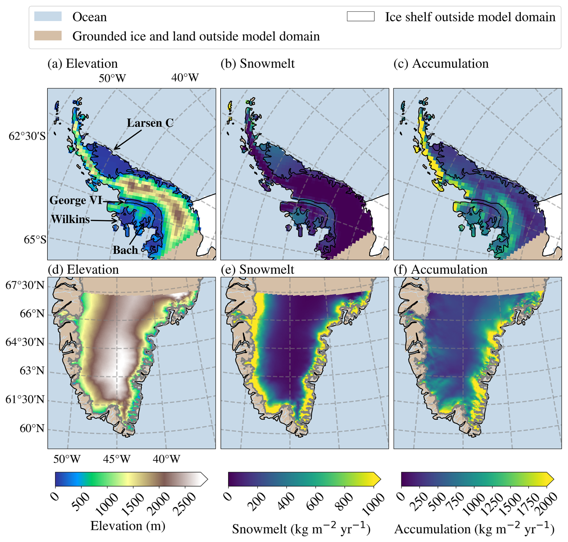
Figure 2 Maps showing elevation (a, d), snowmelt averages (b, e), and accumulation averages (c, f) for the modelled domain in the APIS (a–c) and southern GrIS (d–f) during the spin-up period, i.e. 1979–2020 for the APIS and 1 September 1939–31 December 1970 for the southern GrIS. The black contours show the coastal and ice shelf boundaries in the APIS (a–c) and the coastal boundaries in the southern GrIS (d–f). Ice shelf names within the model domain are indicated for the APIS (a). Gray contours show the ice mask boundaries in southern GrIS (d–f).

In the APIS, the main climate gradient is from the wet and warm west to the dry and cold east. The ice shelves are the lowest-lying areas (Fig. 2a) and experience most snowmelt (up to 500 $\mathrm{kg}{\mathrm{m}}^{-\mathrm{2}}{\mathrm{yr}}^{-\mathrm{1}}$) (Fig. 2b), whereas the snowmelt is limited on the higher-elevated grounded ice. In contrast, the grounded ice has higher accumulation, peaking in the north-west of the APIS. Accumulation is lower on the ice shelves (Fig. 2c).

In the southern GrIS, the lowest-lying marginal areas (Fig. 2d) experience most snowmelt (>750 $\mathrm{kg}{\mathrm{m}}^{-\mathrm{2}}{\mathrm{yr}}^{-\mathrm{1}}$) (Fig. 2e). Accumulation is highest in the east (>2000 $\mathrm{kg}{\mathrm{m}}^{-\mathrm{2}}{\mathrm{yr}}^{-\mathrm{1}}$) (Fig. 2f). Snowmelt rates exceeding 500 $\mathrm{kg}{\mathrm{m}}^{-\mathrm{2}}{\mathrm{yr}}^{-\mathrm{1}}$ combined with high accumulation, as in the southeastern GrIS, typically results in firn aquifers, or, in drier climate zones like the southwest, in ice slabs (Brils et al., 2024).

3 Effect of climate forcing timestep on firn

We look into the FAC for dt_force=3 h and compare this to FAC with larger dt_force. We show that increasing dt_force leads to more firn pore space. We present maps of FAC for different dt_force to understand how climate regimes and dt_force influence the FAC, showing the relevance of identifying the processes responsible for these differences. We discuss how these processes depend on the dt_force and how this affects the depletion or creation of pore space. In this section we focus on the effect on total FAC, an important quantity for retention studies.

In the discussion of these results, we use the following abbreviations: FAC_3 h, FAC_6 h, FAC_1 d, and FAC_1 m correspond to the FAC at dt_force=3 h, 6 h, 1 d, and 1 m respectively. The FAC_3 h compared to FAC simulated at a larger dt_force, is defined as $\mathrm{\Delta }{\text{FAC}}_{\mathrm{6}\mathrm{h}}={\text{FAC}}_{\mathrm{6}\mathrm{h}}-{\text{FAC}}_{\mathrm{3}\mathrm{h}}$, $\mathrm{\Delta }{\text{FAC}}_{\mathrm{1}\mathrm{d}}={\text{FAC}}_{\mathrm{1}\mathrm{d}}-{\text{FAC}}_{\mathrm{3}\mathrm{h}}$, and $\mathrm{\Delta }{\text{FAC}}_{\mathrm{1}\mathrm{m}}={\text{FAC}}_{\mathrm{1}\mathrm{m}}-{\text{FAC}}_{\mathrm{3}\mathrm{h}}$. ΔFAC (without subscript) denotes the difference between FAC_3 h and FAC modelled with larger dt_force. A positive ΔFAC thus indicates more pore space for the larger climate forcing time step.

3.1 FAC_3 h and ΔFAC

Figure 3 shows the FAC_3 h (Fig. 3a and e), ΔFAC_6 h (Fig. 3b and f), ΔFAC_1 d (Fig. 3c and g), and ΔFAC_1 m (Fig. 3d and h) for the APIS and southern GrIS. Figure 3b, c, d, f, g, and h show that FAC_3 h is generally lower than FAC with larger dt_force in both the APIS and southern GrIS. The larger the dt_force becomes, the higher the ΔFAC.

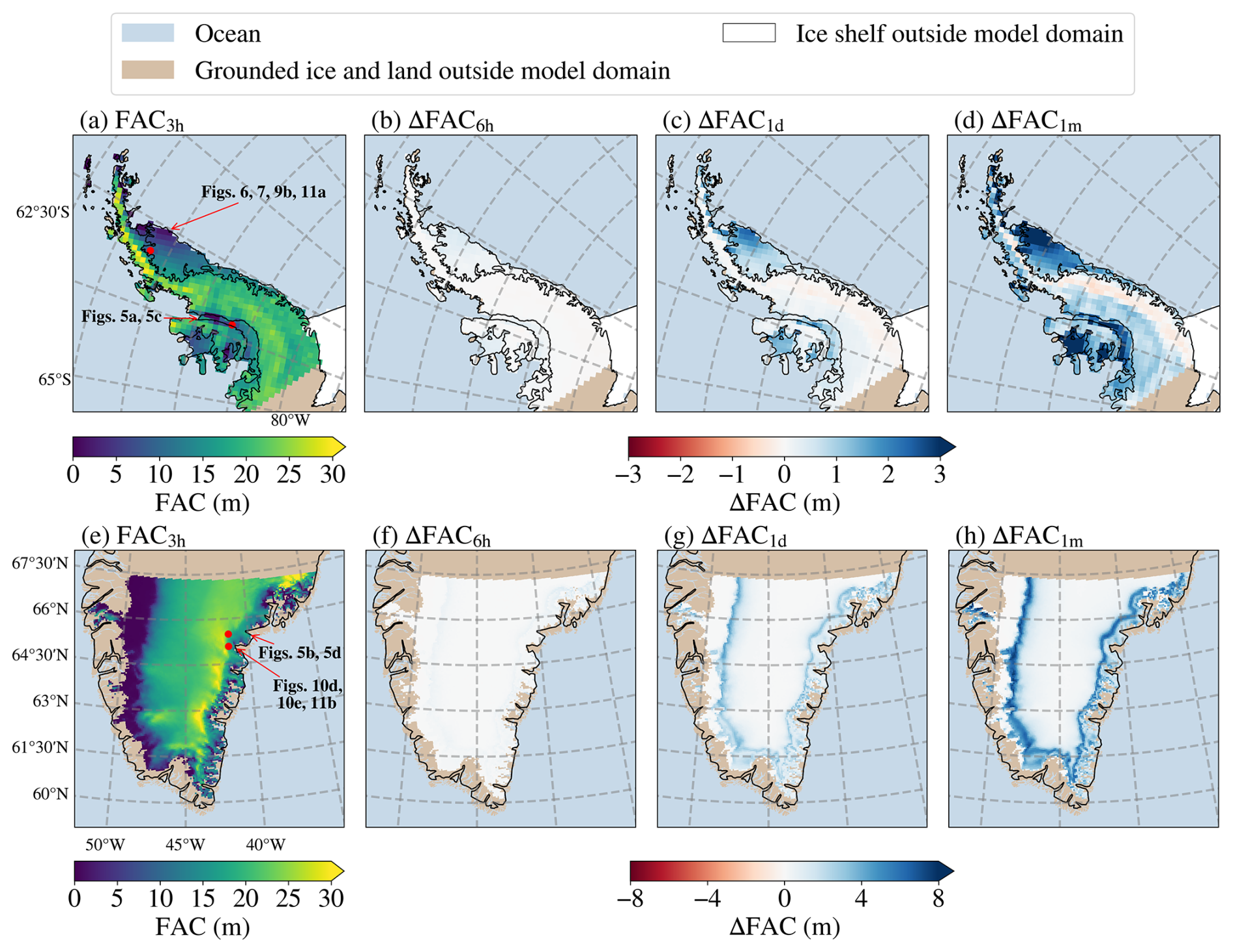
Figure 3 Maps showing average FAC_3 h (a, e), along with average ΔFAC_6 h (b, f), ΔFAC_1 d (c, g), and ΔFAC_1 m (d, h) in the APIS (a–d) and southern GrIS (e–h). The averages are over the whole simulation period, i.e. 1979–2023 for the APIS and 1 September 1939–31 December 2023 for the southern GrIS. The red dots highlighted in panel (a) and (e) are used as example locations later in this paper.

On the APIS, FAC is smallest (0–5 m for FAC_3 h) in the lower-lying areas, corresponding to the ice shelves (Fig. 3a). ΔFAC is largest on the ice shelves (15 % for ΔFAC_1 d, increasing up to 44 % for ΔFAC_1 m). ΔFAC_6 h is relatively small (3 %). Interestingly, an area with a negative ΔFAC is situated along the high-elevation southern spine of the APIS (red hues in Fig. 3b–d). In a relative sense, these differences are small, of the order of ∼0.5 m on typical FAC_3 h values of 15–20 m. In both an absolute and a relative sense, ΔFAC is largest for the locations with low FAC_3 h.

In the southern GrIS, FAC increases from the ice margin where it equals zero in the ablation zone, to higher elevations, with the steepest spatial gradients on the east coast (Fig. 3e). In the southern GrIS, in the ablation zone, most clearly visible on the western margin, ΔFAC is small (Fig. 3f–h). Here, firn pore space is depleted across all simulations, regardless of dt_force. At high elevations (>2000 m), ΔFAC is also relatively small, with average differences <1 % in ΔFAC_6 h up to 3 % in ΔFAC_1 m. At intermediate elevations, a band with larger ΔFAC is apparent, increasing with greater dt_force (Fig. 3f, g, and h). In the east and west, ΔFAC in this band is quite similar in an absolute sense: on average, ΔFAC_6 h=0.3 m, ΔFAC_1 d=2.1 m, and ΔFAC_1 m=4.0 m. However, relative differences are larger in the west, where absolute FAC_3 h values are much smaller (typically <20 m) than in the east (typically >20 m).

3.2 Processes responsible for ΔFAC in IMAU-FDM

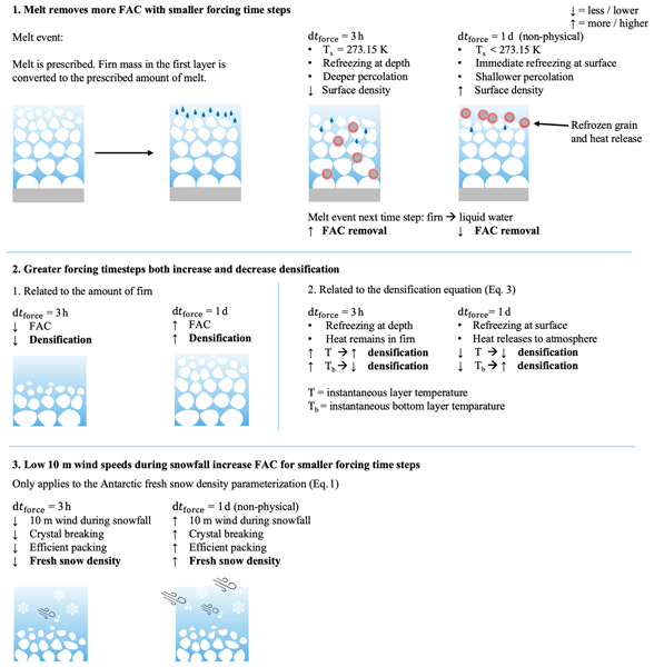
We discuss the processes that contribute to ΔFAC in IMAU-FDM. Figure 4 gives an overview of the dominant processes in a firn layer that cause the forcing time step dependency of the FAC and that are described in depth later in this section. The processes described below are computed every 15 min model time step during both the spin-up and the simulation periods.

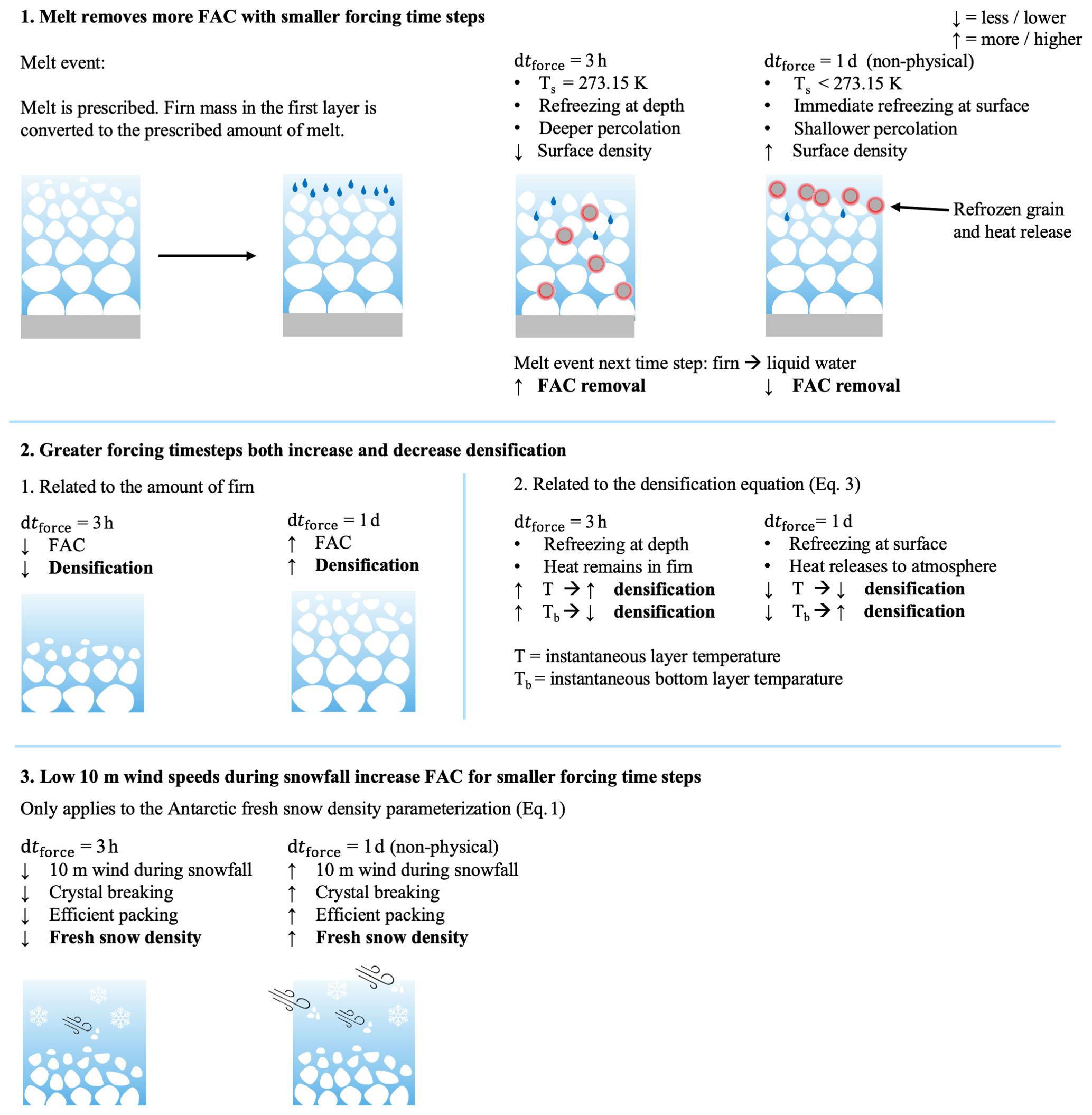
Figure 4 Processes that control (Δ)FAC. The uppermost row shows the effect of a diurnal cycle in dt_force on melt and refreezing, and how those influence FAC. The middle row shows that dt_force can both increase and decrease densification. In the lowermost row, the effect of fresh snow density parameterization in the AIS is shown.

FAC is governed by a balance between the processes that create pore space (snowfall) and that deplete it (densification, snowmelt, snowdrift erosion, and sublimation). Figure 5 shows the relative importance of several processes determining FAC_3 h and FAC_1 d for two example locations depicted in Fig. 3. Figure 5a represents a location in the APIS and Fig. 5b a location in the southern GrIS. Both locations experience similar melt and ΔFAC_1 d, but the location on the GrIS has more snowfall. For clarity, a positive excursion of the elevation change difference in Fig. 5c and d means that the elevation increases more for dt_force=1 d.

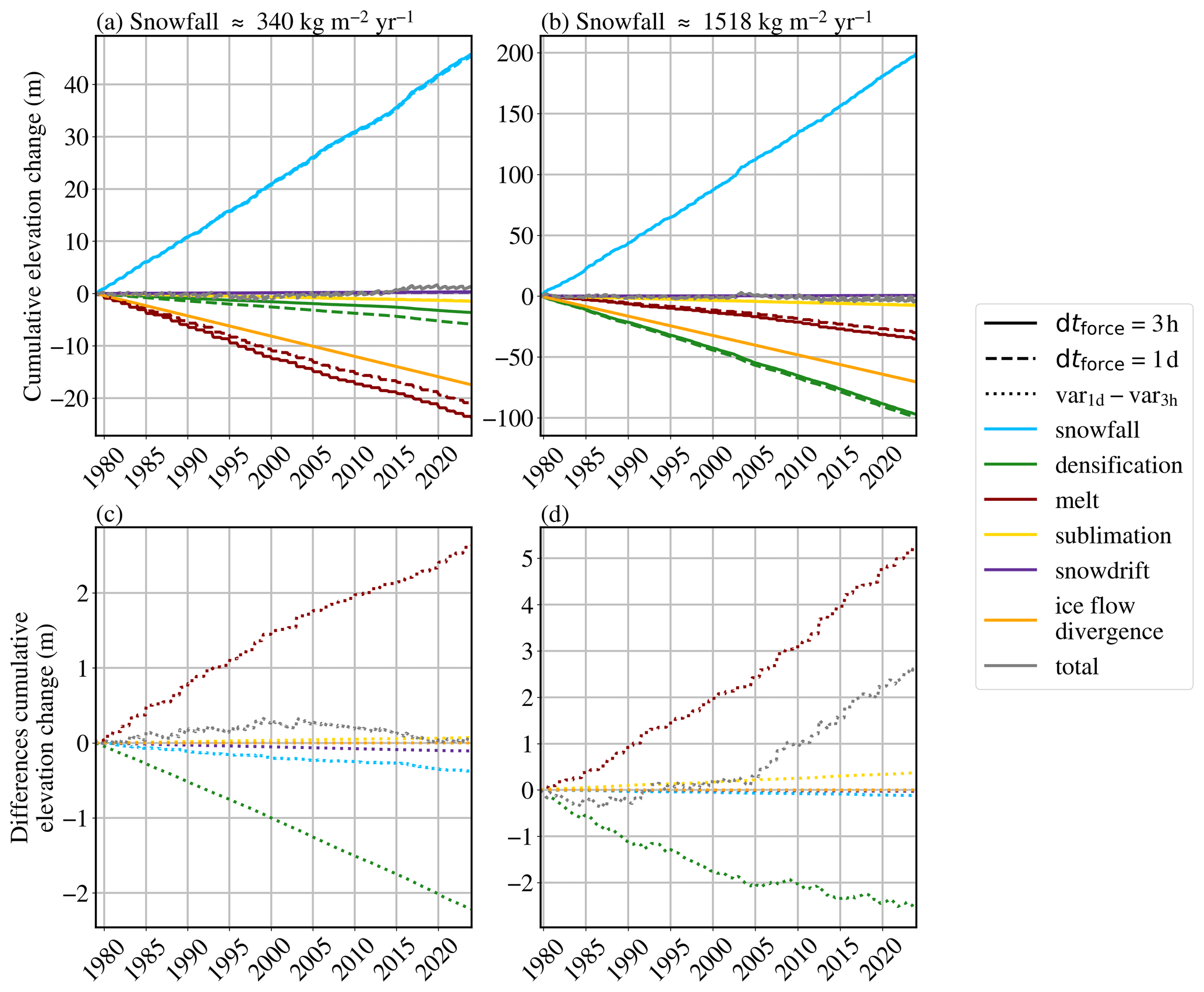
Figure 5 (a) and (b) Cumulative elevation change (m) due to the processes that influence the firn layer. (c) and (d) Differences in cumulative elevation change for all variables between dt_force=1 d and 3 h. Firn densification is integrated over the whole firn column. All other variables represent surface processes. Results for dt_force=3 h are in solid lines, for dt_force=1 d are in dashed lines, and the difference between the two is in dot lines. Panel (a) and (c) are a location in the APIS and panel (b) and (d) are a location in southern GrIS. Both locations experience similar melt (∼340 $\mathrm{kg}{\mathrm{m}}^{-\mathrm{2}}{\mathrm{yr}}^{-\mathrm{1}}$) and ΔFAC_1 d (2.1 m), but different snowfall. See Fig. 3a and e for a map with the grid cell locations.

Snowfall is the major source of firn air in both locations (Fig. 5a and b). The contribution of snowfall to FAC for the APIS is slightly higher for dt_force=3 h than for dt_force=1 d (Fig. 5c), whereas it is almost the same for the GrIS (Fig. 5d). Larger differences arise for processes that reduce FAC. In both locations, more FAC_3 h is removed by snowmelt than FAC_1 d (Fig. 5c and d). For the dry location (Fig. 5a), densification is relatively slow, and FAC depletion due to melt is largest. For the wet location (Fig. 5b), the densification dominates reduction of the FAC. At both locations, melt removes more FAC_3 h and has slower firn densification at dt_force=3 h (Fig. 5c and d).

Summarizing, ΔFAC is mainly controlled by melt and densification rate, with a minor contribution from snowfall. Now, we further zoom in on those processes to understand the ΔFAC they cause.

3.2.1 Process 1: melt

Melt provides the largest contribution to ΔFAC, simulations with dt_force=3 h have more FAC reduction than for larger dt_force (Fig. 5c and d). Climate zones with more melt, have a higher ΔFAC. We identify two types of melt-related mechanisms responsible for ΔFAC, namely a surface-based process and a process occurring at depth.

At the surface, the model is forced with a melt flux, and firn in the top layer is converted to liquid water. The subsequent fate of the meltwater depends on dt_force. With a diurnal cycle in dt_force, i.e. 3- and 6 h, surface temperatures reach 0 °C during melt events. Therefore, the water cannot immediately refreeze and the timing of refreezing and snowmelt in the top layer alternate between day and night (Fig. 6a). In contrast, without a diurnal cycle in dt_force, i.e. 1 d and 1-month, surface melt and temperature become decoupled. As a result, melt can occur at subfreezing surface temperatures and the meltwater that can be retained in the pore space refreezes immediately near the surface (Fig. 6b). This leads to a higher near-surface density under larger dt_force (Fig. 6c). Subsequent melt events convert firn to liquid water again and remove less pore space when a high-density surface layer is present, as in dt_force=1 d and 1 m. This melt and surface temperature interaction in absence of a daily cycle is the main mechanism that leads to higher ΔFAC with increasing dt_force (Fig. 4, process 1).

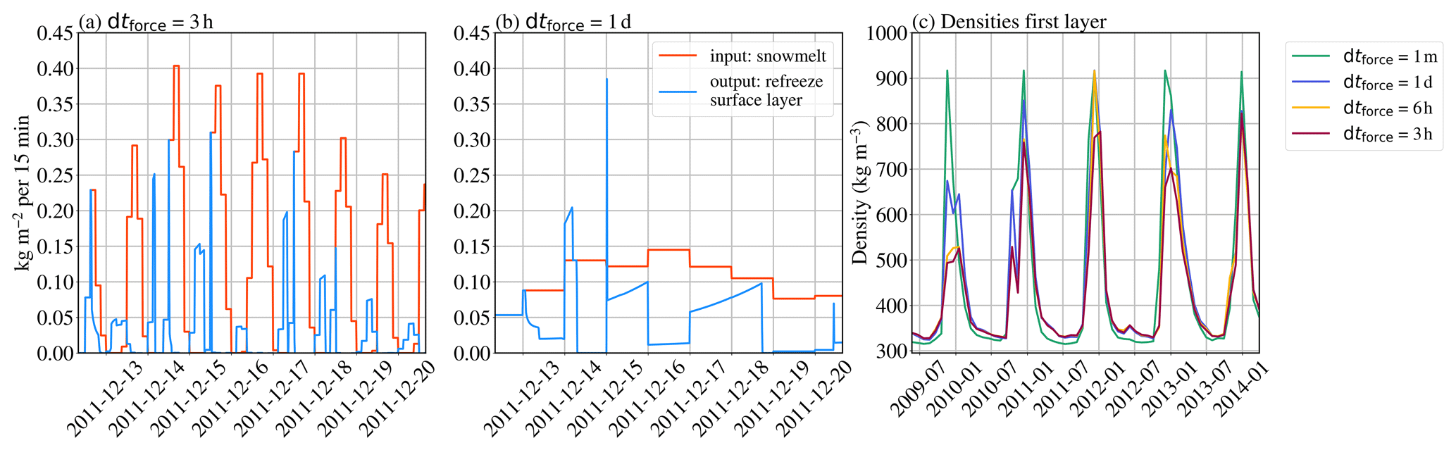
Figure 6 Snowmelt input and modelled refreezing in the surface layer for dt_force=3 h (a) and for dt_force=1 d (b). Panel (c) shows the modelled densities in the surface layer. See Fig. 3a for a map with the grid cell location.

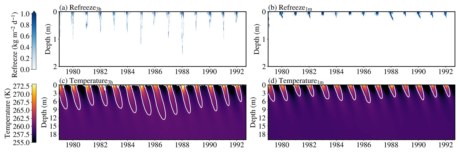
The second process is that meltwater percolates deeper at dt_force=3 h; less water that can be retained in the pore space is immediately refrozen near the surface. Consequently, refreezing occurs deeper if there is enough cold content (Figs. 7a and b and 4 process 1). The latent heat released by refreezing at depth is trapped due to the low thermal conductivity of firn. Thus, the deeper firn for dt_force=3 h is warmer (Fig. 7c and d). Warmer firn enhances firn densification, as discussed in the following subsection.

Figure 7 Refreezing amount and depth (a, b) and temperature profiles (c, d) for an example point on the APIS for dt_force=3 h (a, c) and for dt_force=1 m (b, d). The white contours in panels (c) and (d) represent a temperature of 260 K. See Fig. 3a for a map with the grid cell location.

3.2.2 Process 2: firn densification

Several processes contribute to the firn densification rate. First, more snowfall leads to more firn that can densify (contribution of snowfall to $\dot{b}$ in Eq. 3). Simulations with larger dt_force have more FAC (Fig. 3), and therefore undergo more densification (Figs. 5 and 4, process 2).

Second, the densification rate is governed by the instantaneous layer temperature (T in Eq. 3) and the temperature of the bottom layer (T_b in Eq. 3), with higher T enhancing densification and higher T_b reducing it (Fig. 4, process 2). A similar increase in T and T_b would lead to enhanced densification (see constants in Eq. 3). Because the simulation with dt_force=3 h has deeper refreezing (Fig. 7a compared to Fig. 7b) and warmer firn (Fig. 7c compared to Fig. 7d), the densification is indeed faster. An exception occurs when T is similar for different dt_force for the uppermost meters of the firn column, but T_b is higher for dt_force=3 h due to the deeper refreezing. Then the larger approximated grain size for dt_force=3 h slows down the densification rate, leaving more FAC.

To summarize, higher firn temperatures at dt_force=3 h increase densification rate. However, the reduction in firn depth resulting from densification (Fig. 5) remains smaller as less pore space is available to densify.

3.2.3 Process 3: fresh snow density on the APIS

An area with lower rather than higher ΔFAC is modelled in the APIS (red hues in Fig. 3b–d); this relates to differences in the estimated fresh snow density for various dt_force. The simulation for dt_force=3 h has higher 10 m wind speed (ff_10 m) variability than for larger dt_force, which influences fresh snow density through Eq. (1): fresh snow density increases with surface temperature T_s (Judson and Doesken, 2000) and ff_10 m (Sato et al., 2008). The area with negative ΔFAC typically experiences snowfall at low ff_10 m. Lower wind speeds during snowfall lead to less crystal breaking, and therefore, less efficient packing at the surface, decreasing the fresh snow density (Fig. 4, process 3). Then, the snowfall-weighted average 10 m wind speed (${\stackrel{\mathrm{‾}}{\mathit{ff}\mathrm{10}\mathrm{m}}}^{\text{sf}}$) (Eq. 4) for dt_force=3 h is lower than for larger dt_force (Fig. 8).

$$\begin{array}{}\text{(4)}& {\displaystyle }{\displaystyle }{\stackrel{\mathrm{‾}}{\mathit{ff}\mathrm{10}\mathrm{m}}}^{\text{sf}}={\displaystyle \frac{\sum \text{snowfall}\left(t\right)\times {\mathit{ff}}_{\mathrm{10}\mathrm{m}}\left(t\right)}{\sum \text{snowfall}\left(t\right)}}\end{array}$$

Thus, lower ${\stackrel{\mathrm{‾}}{\mathit{ff}\mathrm{10}\mathrm{m}}}_{\mathrm{3}\mathrm{h}}^{\text{sf}}$ is related to lower fresh snow densities, and therefore higher FAC_3 h. In climate zones with limited melt (<30 $\mathrm{kg}{\mathrm{m}}^{-\mathrm{2}}{\mathrm{yr}}^{-\mathrm{1}}$), this effect of the fresh snow density causes a relatively small and possible negative ΔFAC of up to ±0.5 m on typical FAC_3 h values of 15–20 m (Fig. 3a–d).

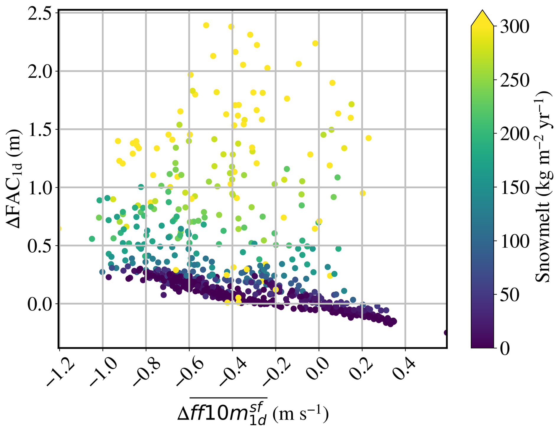
Figure 8 The ΔFAC_1 d against $\mathrm{\Delta }{\stackrel{\mathrm{‾}}{\mathit{ff}\mathrm{10}\mathrm{m}}}_{\mathrm{1}\mathrm{d}}^{\text{sf}}$ in the APIS. $\mathrm{\Delta }{\stackrel{\mathrm{‾}}{\mathit{ff}\mathrm{10}\mathrm{m}}}_{\mathrm{1}\mathrm{d}}^{\text{sf}}={\stackrel{\mathrm{‾}}{\mathit{ff}\mathrm{10}\mathrm{m}}}_{\mathrm{1}\mathrm{d}}^{\text{sf}}-{\stackrel{\mathrm{‾}}{\mathit{ff}\mathrm{10}\mathrm{m}}}_{\mathrm{3}\mathrm{h}}^{\text{sf}}$. In absence of melt, there is a clear relation between $\mathrm{\Delta }{\stackrel{\mathrm{‾}}{\mathit{ff}\mathrm{10}\mathrm{m}}}_{\mathrm{1}\mathrm{d}}^{\text{sf}}$ and ΔFAC_1 d.

Figure 9 (a) Average ΔFAC_6 h, ΔFAC_1 d, and ΔFAC_1 m over the simulation period against average snowmelt over 1979–2020. (b) FAC timeseries of one grid point on the APIS for the four dt_force. See Fig. 3a for a map with the grid cell location.

4 Implications for IMAU-FDM

Climatic differences between the APIS and southern GrIS lead to a different response of ΔFAC to dt_force in IMAU-FDM. Moreover, the APIS primarily experiences a steady state climate, whereas the southern GrIS climate starts changing after 1990. The dt_force has different implications for steady and changing climates. Lastly, ΔFAC modifies the firn correction to altimetry. The climate and altimetry implications are discussed in the following sections for both ice sheets.

4.1 APIS

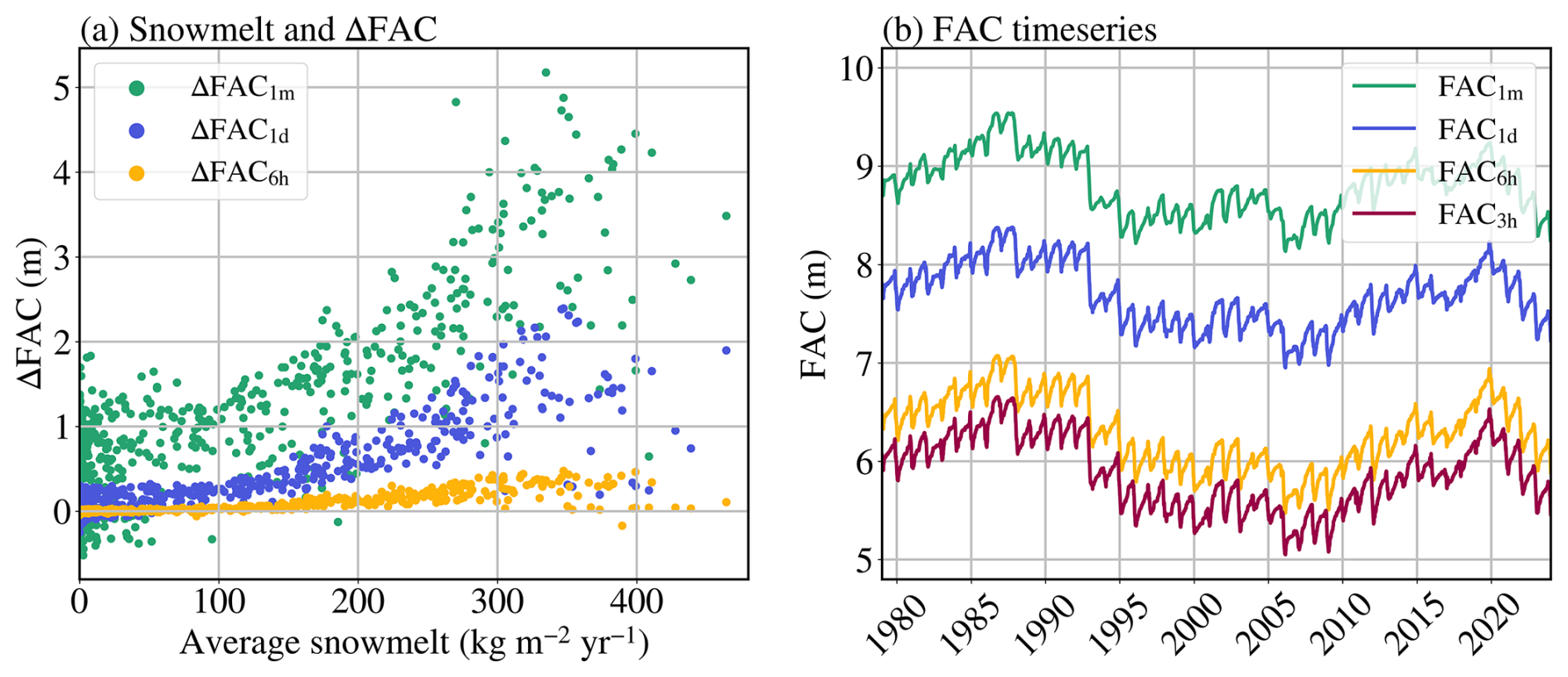
Figure 9a shows that ΔFAC on the APIS increases with snowmelt. Accordingly, ice shelves have largest positive ΔFAC values (Fig. 3b–d), reflecting their relatively high snowmelt rates (Fig. 2b). Consequently, the chosen dt_force is crucial in assessing whether the firn air is depleted or could still buffer meltwater. Ice shelves are more vulnerable to hydrofracturing when the firn air is depleted. Therefore, neglecting the daily temperature and melt cycle in firn simulations could lead to underestimated ice shelf vulnerability.

Figure 9b presents a FAC timeseries of a single grid cell on the Larsen C ice shelf (see Fig. 3 for location). The overall variations in FAC are similar across all simulations, with ΔFAC primarily established during the spin-up. The equilibrium state of the firn column has higher FAC for larger dt_force, where reduced FAC removal during melt events is balanced by enhanced densification.

4.2 Southern GrIS

The wider range of climatic conditions in terms of snowmelt and accumulation in the southern GrIS (Fig. 10a) compared to the APIS (Fig. 9a), complicates the isolation of processes governing ΔFAC. To facilitate the discussion, we divide the accumulation-snowmelt space into four domains (Fig. 10a).

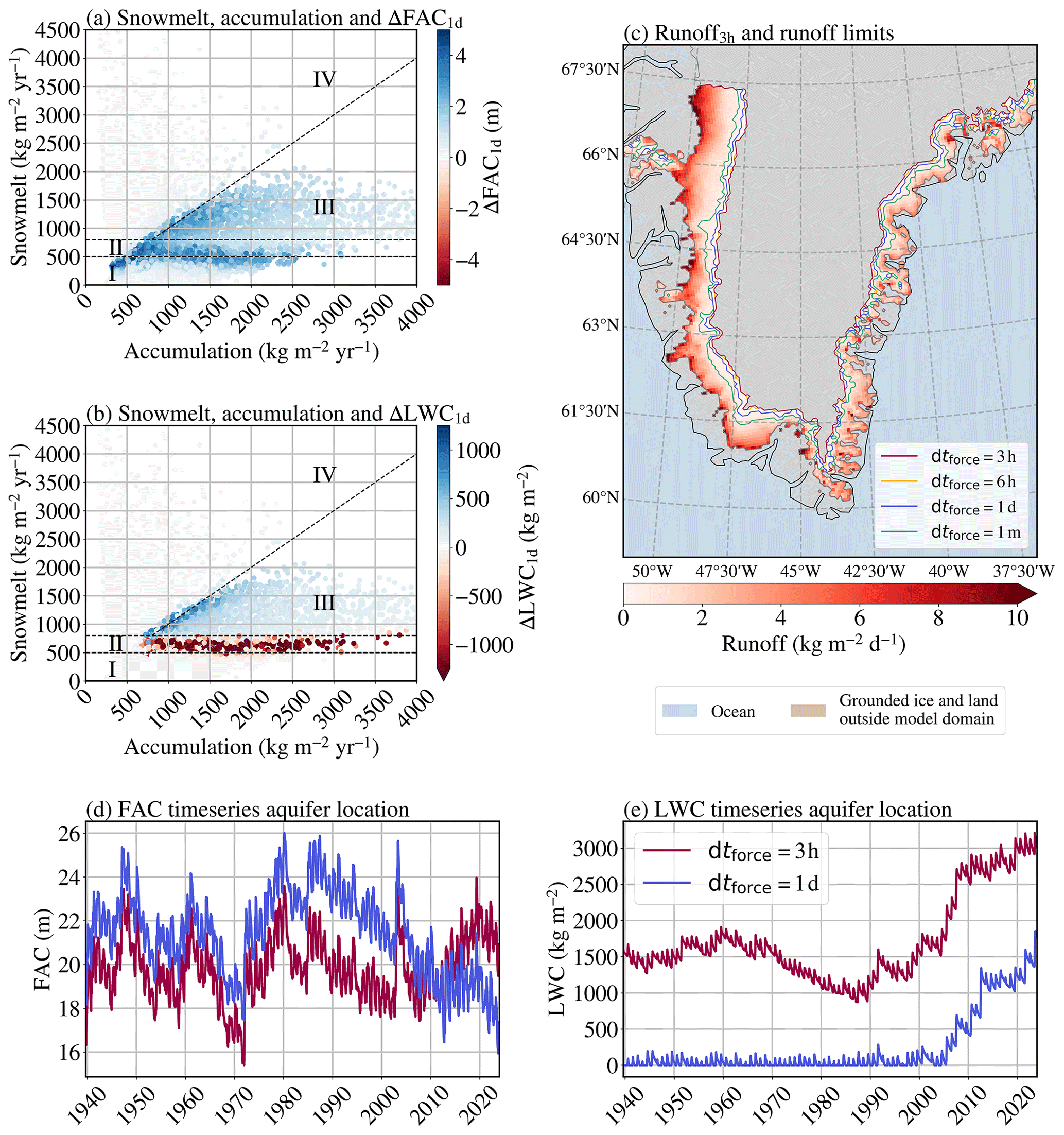
Figure 10 Average snowmelt against accumulation over 1939–1970 colour coded with average ΔFAC_1 d (a) and ΔLWC_1 d (b) over the simulation period. The black dashed lines represent snowmelt of 500 $\mathrm{kg}{\mathrm{m}}^{-\mathrm{2}}{\mathrm{yr}}^{-\mathrm{1}}$ (climate zone I), 500–800 $\mathrm{kg}{\mathrm{m}}^{-\mathrm{2}}{\mathrm{yr}}^{-\mathrm{1}}$ (climate zone II) and a MOA of 1 (separating climate zones III and IV). Panel (c) shows the average runoff_3 h over the simulation period and the different runoff limits for the four dt_force. Panel (d) and (e) show timeseries of respectively FAC_3 h and FAC_1 d, and LWC_3 h and LWC_1 d. See Fig. 3e for a map with the grid cell location.

The largest increases in ΔFAC_1 d occur at snowmelt rates of ∼500 $\mathrm{kg}{\mathrm{m}}^{-\mathrm{2}}{\mathrm{yr}}^{-\mathrm{1}}$ and near a Melt-Over-Accumulation (MOA) ratio of 1 (Fig. 10a). Climate zones with snowmelt below 500 $\mathrm{kg}{\mathrm{m}}^{-\mathrm{2}}{\mathrm{yr}}^{-\mathrm{1}}$ (Fig. 10a, climate zone I), corresponding to the interior of the southern GrIS (Fig. 2e), behave similarly to the APIS: higher snowmelt rates increase ΔFAC_1 d.

Firn aquifers can form when snowmelt exceeds 500 $\mathrm{kg}{\mathrm{m}}^{-\mathrm{2}}{\mathrm{yr}}^{-\mathrm{1}}$ (Kuipers Munneke et al., 2014; Brils et al., 2024). In climate zone II (Fig. 10a and b), which are the points with annual snowmelt between 500–800 $\mathrm{kg}{\mathrm{m}}^{-\mathrm{2}}{\mathrm{yr}}^{-\mathrm{1}}$, firn aquifers formed under dt_force=3 h during spin-up, but did not for dt_force=1 d. The firn has a higher heat content throughout the entire column for dt_force=3 h, due to the deeper refreezing of meltwater. The higher heat content limits the refreezing capacity. We hypothesize that more liquid water remains in the firn layer and the aquifer can refill during the next melt season. In contrast, the cold content for dt_force=1 d still facilitates refreezing of all liquid water, and therefore, aquifers did not form during spin-up.

In climate zone III, snowmelt exceeds 800 $\mathrm{kg}{\mathrm{m}}^{-\mathrm{2}}{\mathrm{yr}}^{-\mathrm{1}}$ and the MOA is below 1. Firn aquifers form under both dt_force=3 h and 1 d (Fig. 10b). Here, ΔFAC_1 d increases with snowmelt as less pore space is removed for larger dt_force (Fig. 4, process 1), but this process is increasingly counterbalanced by enhanced firn densification at sites with higher accumulation (Fig. 10a). FAC_3 h is lower in this climate zone, so less pore space is available for water storage, resulting in less liquid water content (LWC) for dt_force=3 h whereas the liquid water is still retained for dt_force=1 d (Fig. 10b). More excess water for dt_force=3 h leads to more runoff. This example illustrates that the runoff limit also depends on dt_force (Fig. 10c). In the southeastern GrIS, the runoff limit shifts more than 10 km inland for dt_force=3 h compared to dt_force=1 d, and up to 35 km compared to dt_force=1 m. This result shows that dt_force plays a role in estimates of future GrIS mass balance projections.

When the MOA exceeds 1 (Fig. 10a climate zone IV), ΔFAC equals 0, as the firn is depleted in both simulations.

Unlike the example of the APIS (Fig. 9b), long-term FAC variability in Fig. 10d depends on dt_force (Fig. 10d). For dt_force=3 h, firn aquifers are present at the start of the simulation, whereas for dt_force=1 d they develop around 2005 (climate zone II) (Fig. 10e). In this year, the change in FAC_1 d diverges from FAC_3 h, and eventually, FAC_1 d even drops below FAC_3 h. This results from the densification equation (Eq. 3): liquid water in the aquifers sets the instantaneous temperature (T in Eq. 3) to 273.15 K. The bottom temperature (T_b in Eq. 3) is higher for dt_force=3 h (Sect. 3.2.1), because of the deeper refreezing, slowing down densification. The faster densification under dt_force=1 d reduces FAC_1 d. Hence, for locations where aquifers form during the simulation, the time series of FAC (and surface elevation) become different and their trends possibly of opposite sign. This has important implications for the correct interpretation of satellite altimetry.

4.3 Implications for steady state and changing climates

Figure 9b shows an example from the APIS where the FAC differences due to dt_force are established during the spin-up period (1979–2020), during which the climate is assumed to be in an approximate steady state. The simulation continues for only three more years. Therefore, the ΔFAC for this location is mainly established during the spin-up period. Figure 10d shows a GrIS aquifer location, where ΔFAC develops both during and after the spin-up, which ends in 1970. The changing climate after 1970 causes FAC_3 h and FAC_1 d variations to diverge further. In this example, the ΔFAC divergence is associated with the formation of firn aquifers.

Figure 11 Differences in surface height changes over time between dt_force=3 h and larger climate forcing time steps. Panel (a) represents the point in Fig. 9b and (b) the point in Fig. 10d and e. See Fig. 3e for a map with the grid cell location.

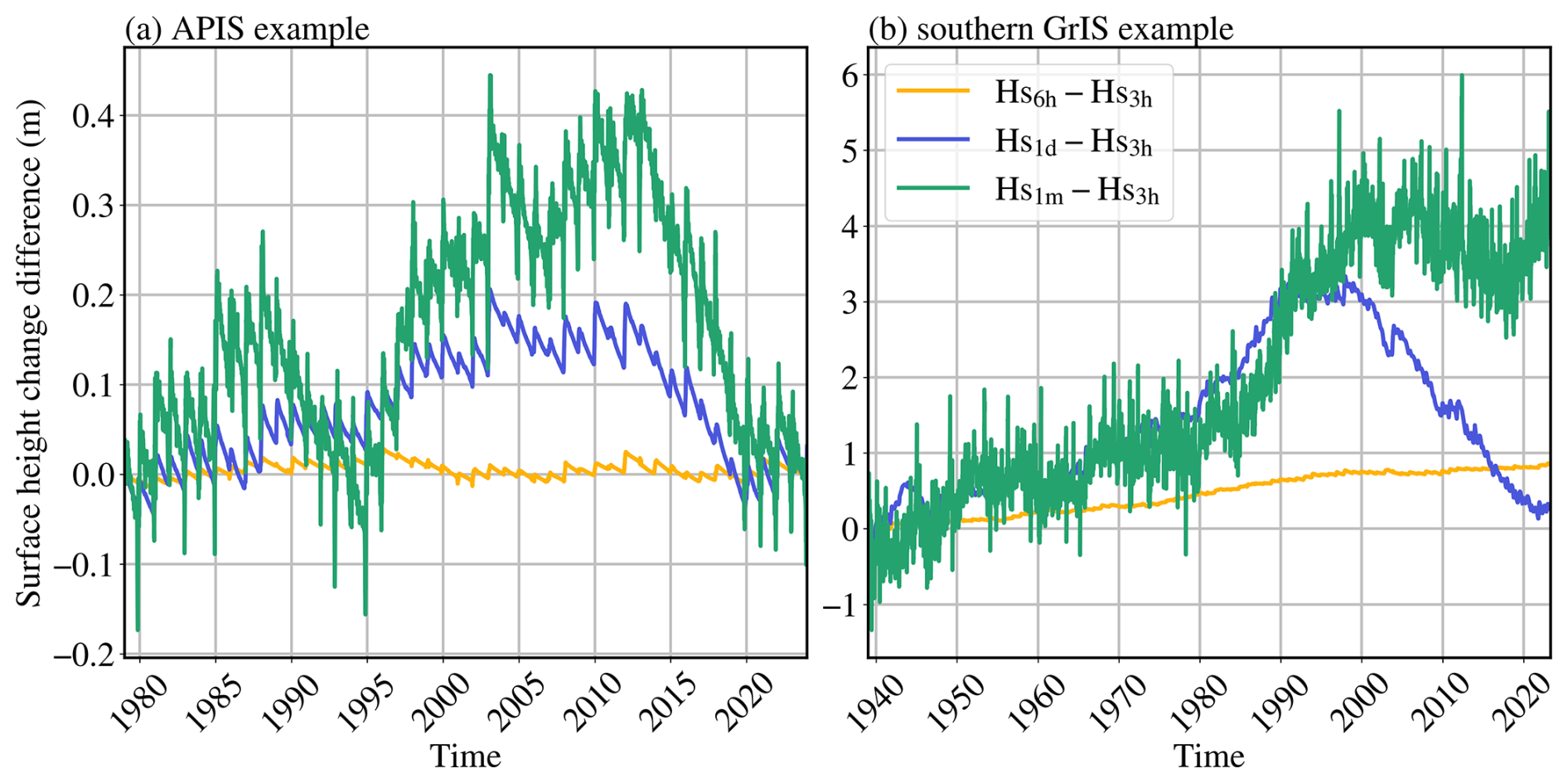
Figure A1 shows the spatial distribution of ΔFAC_1 m during the last year of the simulation without the contribution from the spin-up period. The magnitude of ΔFAC established after the spin-up is larger on the GrIS than on the APIS, because the GrIS simulation covers a larger period with a changing climate. In addition, on the GrIS, the changing climate leads to formation of firn aquifers, causing the FAC to diverge after the spin-up under different dt_force (Fig. 10d and e). The mechanisms described in Sect. 3.2 lead to the ΔFAC differences established both during and after the spin-up.

4.4 Altimetry corrections

As simulated FAC depends on dt_force, then so does firn depth and hence surface height change, which is in turn used to correct altimetry data. For the same APIS sample location as shown in Fig. 9b, surface height change under dt_force=1 d and 1 m differs from dt_force=3 h by 0.2 and 0.4 m, respectively (Fig. 11a). ΔFAC already emerges during spin-up. At a GrIS location in transition to an aquifer, as shown in Fig. 10d and e, ΔFAC is primarily established after the spin-up and shows a stronger divergence of surface height changes, at 8 %–30 % of the FAC (Fig. 11b). Altimetry corrections based on IMAU-FDM simulations with dt_force=1 d and 1 m would give higher surface height increases for the two examples. Consequently, during periods of ice thinning, subtracting the modeled firn depth change from the altimetry signal leads to an underestimation of ice loss, while during periods of ice thickening it leads to an underestimation of ice gain.

5 Lessons learned for firn modelling

In this section we present the lessons learned of using different dt_force in firn modelling. We distinguish between findings specific to IMAU-FDM and general findings.

Firn models that prescribe snowmelt fluxes and surface temperature, like IMAU-FDM, need at least a diurnal cycle in the dt_force. Snowmelt is the major predictor of ΔFAC, increasing ΔFAC for larger dt_force. Without resolving the daily cycle, snowmelt can co-exist with subfreezing surface temperatures, leading to immediate refreezing of the meltwater that is retained in the layer. This decoupling of surface temperature and snowmelt leads to non-physical results. Firn models with surface energy balance schemes that compute rather than prescribe melt fluxes might be less sensitive to this finding, but might suffer from less accurate melt fluxes.

Second, we showed how the fresh-snow density and densification parameterizations in IMAU-FDM are sensitive to dt_force. The fresh-snow density parameterization (Eq. 1) in the APIS is tuned specifically using dt_force=3 h (Veldhuijsen et al., 2023). ΔFAC arising from other dt_force are related to the wrong use of the parameterization (Fig. 8) and are not based on physical grounds. The densification equation (Eq. 3) is based on steady state and assumes dry, non-melting snow. However, we applied the parameterization also for transient and wet conditions. The latter results in non-physical processes where the bottom temperature (T_b in Eq. 3) determines the densification rate in an aquifer and leads to different FAC variations over time for different dt_force (Fig. 10d and e). A general lesson learned for modelling is that the original purpose and forcing time step of a parameterization should be respected.

6 Conclusions

Ice-sheet firn models use different surface climate forcing time steps. In this study we investigated the effect of using a 3 , 6 h, 1 d, and 1-month climate forcing time step on firn air content modelled by IMAU-FDM in the Antarctic Peninsula and southern Greenland Ice Sheet.

We find that increasing the climate forcing time step typically results in more firn air (positive ΔFAC). The magnitude of this change depends on the climate regime and is most sensitive to snowmelt. More specifically, the climate forcing should resolve the diurnal cycle when surface temperature and snowmelt are prescribed at the top boundary. Otherwise, subfreezing temperatures and snowmelt can coexist, leading to immediate refreezing of the retained meltwater and, consequently, overestimating the amount of firn air.

We found that in IMAU-FDM, ΔFAC increases with snowmelt for melt rates up to 500 $\mathrm{kg}{\mathrm{m}}^{-\mathrm{2}}{\mathrm{yr}}^{-\mathrm{1}}$, across both the APIS and southern GrIS. In the latter, snowmelt rates exceeding 500 $\mathrm{kg}{\mathrm{m}}^{-\mathrm{2}}{\mathrm{yr}}^{-\mathrm{1}}$ can lead to the formation of firn aquifers. A smaller climate forcing time step results in earlier aquifer formation and therefore higher ΔFAC. Once aquifers have formed ΔFAC increases with snowmelt up to a melt-over-accumulation rate of 1, above which the firn becomes depleted for all climate forcing time steps.

In IMAU-FDM, ΔFAC was also caused by the densification and fresh snow density parameterization for non-physical reasons, i.e. when the original purpose and temporal resolution of the original parameterizations is not respected.

Ice-sheet firn air content impacts the interpretation of altimetry observations, co-determines the ice-sheet meltwater retention potential and therewith runoff limits and ice shelf vulnerability to hydrofracturing. In firn models, the climate forcing time step potentially influences the simulated firn air content and should therefore be carefully selected and tested.

Appendix A: Implications steady state and changing climate maps

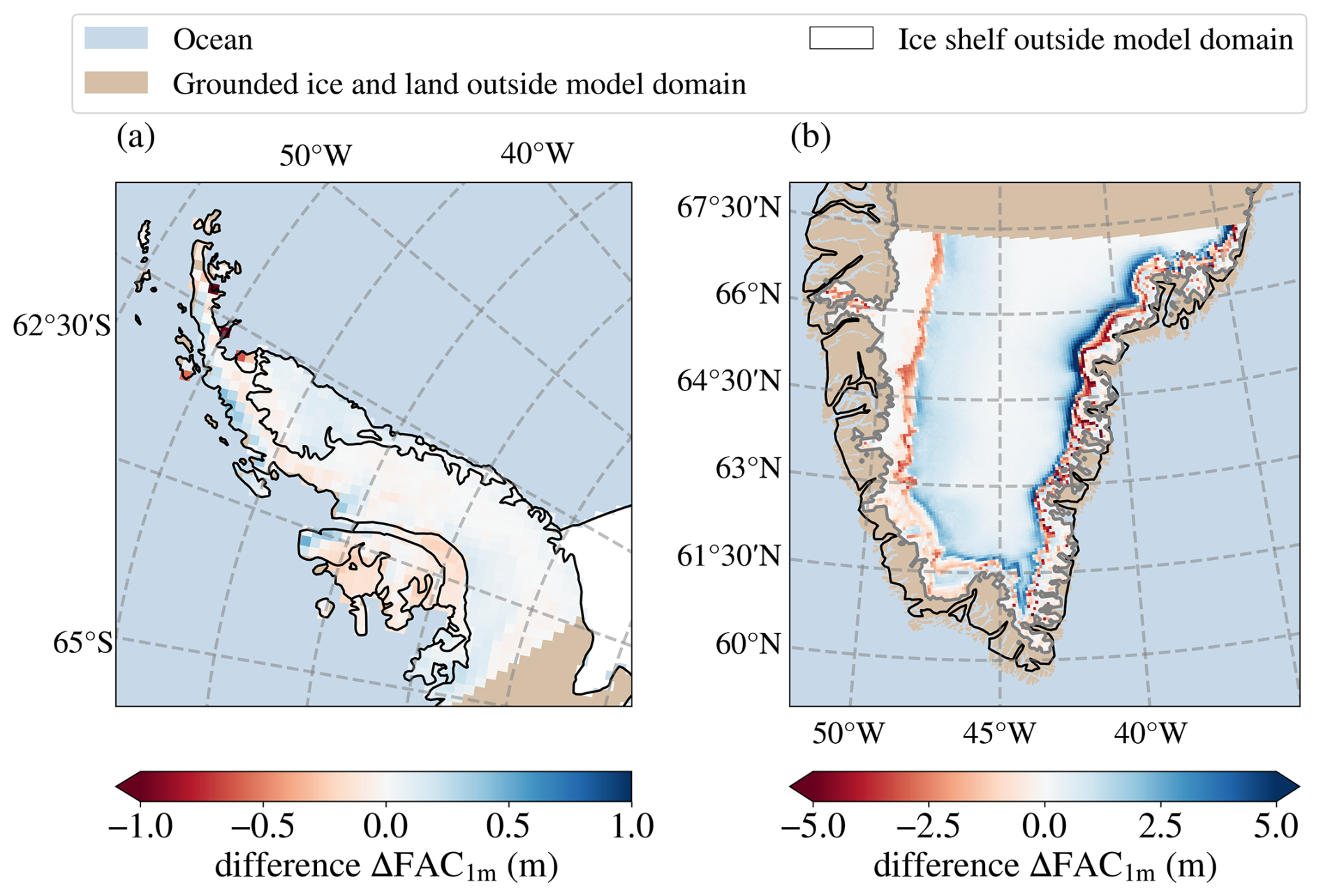
Figure A1 Differences in ΔFAC_1 m between the last simulation year and the first simulation year for the APIS (a) and southern GrIS (b). Red colours indicate that ΔFAC_1 m was larger during the first simulation year, directly after the spin-up. Blue colours indicate that ΔFAC_1 m was larger during the last simulation year.