Feedbacks and timescales in the modelled transient response of debris-covered glaciers

Glaciers worldwide are becoming increasingly debris-covered, yet many aspects within the coupled glacier-debris system are not well-understood. While the insulating effect of continuous debris layers is well-known, the transient feedbacks with glacier dynamics are poorly understood. The main aim of this study is to better understand the complex transient glacier response and debris-induced feedbacks through numerical flow modelling. We present an improved flowline model that couples ice flow, depth-resolved debris transport, and debris cover impact on mass balance. This approach allows for a detailed examination of the dynamics of debris-covered glaciers under transient forcing conditions of climate and debris input over extended timescales. Our results indicate that low-amplitude, decade-scale variability in debris or climate forcing does not substantially impact glacier evolution. However, large debris supply events can have a sustained impact. We find that debris-covered glacier response to warming climate forcing is non-monotonic, with distinct phases of thinning, retreat, and long-term re-advance. We attribute this to a separate, longer timescale process of englacial debris transport. Additionally, feedbacks in the englacial debris trajectory and complex bed topography further amplify the non-linear pattern of retreat in the transient glacier response to warming.

1 Introduction

Debris-covered glaciers are found in all glaciated mountain ranges and are particularly common in high relief mountain areas. In recent years, there has been growing interest in debris-covered glaciers, as under the current warming, the number of debris-covered glaciers and their percentage of debris-covered area is substantially increasing (Anderson, 2000; Kirkbride and Deline, 2013). A multitude of studies have attempted to represent the evolution of debris-covered glacier systems in numerical models (e.g., Konrad and Humphrey, 2000; Banerjee and Shankar, 2013; Rowan et al., 2015; Anderson and Anderson, 2016; Scherler and Egholm, 2020; Ferguson and Vieli, 2021; Mayer and Licciulli, 2021; Verhaegen and Huybrechts, 2026). Yet we do not fully understand many elements and interactions of the debris-covered glacier system in a changing climate. This includes, for example, the effect from variations in debris supply from headwalls, processes influencing supraglacial debris re-distribution and morphology, and terminus processes (Nicholson et al., 2021).

Debris cover is, above a thickness of a few centimeters, known to protect the ice from surface ablation (e.g., Østrem, 1959; Mattson et al., 1993; Miles et al., 2022; Laha et al., 2023; Fontrodona-Bach et al., 2025) and thereby changes the spatial patterns of surface mass balance compared to those on debris-free “clean-ice” glaciers (Nicholson and Benn, 2006). A continuous debris cover on the surface therefore reduces the ablation there and leads to today's typically observed, extended debris-covered glacier tongues (Benn et al., 2012; Kirkbride and Deline, 2013; Carturan et al., 2013). Considering debris thickness and its insulating effect statically is, however, not sufficient for understanding the evolution of debris-covered glaciers, as the debris is being transported along and within the glacier and hence its thickness is strongly linked to ice dynamics. A more dynamically active glacier may, for example, lead to thinner debris thicknesses as the debris has less time to accumulate on the surface (Anderson et al., 2021). Debris thickness also depends on the rate and location of debris input to the glacier. Furthermore, any perturbation in forcing (climate or debris) is followed by a delayed glacier response (Bahr et al., 1998). This is true for any glacier, but debris adds an additional element that leads to a response involving multiple timescales that have remained largely unexplored (Ferguson and Vieli, 2021).

As debris can be transported both englacially or supraglacially, understanding the transport paths and interaction with flow dynamics is essential for improving our understanding of the entire system. Due to the reduced ablation on debris-covered tongues, dynamic adjustments in glacier length are expected to be slower, on a century rather than a decadal timescale, and hence mostly beyond the observational record (Ferguson and Vieli, 2021).

To better understand the evolution and dynamic feedbacks in the debris-covered glacier system, it is therefore crucial to dynamically couple the involved processes from debris input, its transport, glacier flow, debris thickness evolution, and its effect on surface mass balance. Further, we need to consider the transient response of the debris-covered glacier system to a variable climate and debris input, beyond the observational record. Numerical flow modelling allows for quantitatively coupling and evolving ice flow, glacier and debris evolution. A limited number of dynamic modelling studies have attempted to do this (e.g., Rowan et al., 2015; Verhaegen et al., 2020; Compagno et al., 2022). However, they vary strongly in the way they include the effects of debris and its interaction with glacier flow, depending on the research questions to be addressed and the related simplifications made.

There are three main approaches of treating debris in transient glacier flow models. The first set of models prescribe the spatial debris thickness patterns on the surface in order to account for their reduction on ablation without explicitly considering debris transport (Banerjee and Shankar, 2013; Compagno et al., 2022). A second set of models includes, in addition to the effect of debris on ablation, the linking of supraglacial debris flux to surface velocity (Vacco et al., 2010; Verhaegen et al., 2020; Ferguson and Vieli, 2021; Mayer and Licciulli, 2021), but assumes spatially uniform debris concentration with the ice. The third set of models includes an explicit treatment of englacial debris by transporting the debris through the glacier using either an Eulerian approach, advecting debris concentration on a grid (Rowan et al., 2015, 2021; Anderson and Anderson, 2016; Wirbel et al., 2018; Ferguson, 2022; Verhaegen and Huybrechts, 2026), or by tracking debris as Lagrangian particles (e.g., in the integrated second-order Shallow Ice Approximation model iSOSIA: Egholm et al., 2011; Scherler and Egholm, 2020; Margirier et al., 2025). However, these models have not systematically investigated time transient aspects in forcing.

The main novelties of this study are the examination of both temporally variable debris input and transient climate forcing to debris-covered glacier evolution and an in-depth analysis of the involved feedbacks, and response times from the related englacial debris transport. We present a numerical flow model that couples ice and debris dynamics to examine the combined effects and feedbacks in the debris-covered glacier system. Our approach unites many elements from existing studies, using a flowline model with depth-resolved (2D) Eulerian debris transport as in Anderson and Anderson (2016). Our approach introduces a novel debris entrainment implementation that allows to independently control climate and debris forcing for exploring the transient feedbacks between them. Further, the model includes the separation of detached ice masses, which is becoming increasingly common for glaciers, in particular with complex bed topography (Pellicciotti et al., 2015; Rippin et al., 2020; Rowan et al., 2021). To examine the validity of our model, we perform benchmark experiments as conducted in previous approaches (Anderson and Anderson, 2016; Ferguson and Vieli, 2021; Ferguson, 2022), but our main focus lies on exploring the fundamental relationships that govern the geometry of debris-covered glaciers, depending on debris supply, ELA, and topography. We investigate the non-linear dynamic response to warming that is specific to debris-covered glaciers and the effect and timescales resulting from a variable debris supply. One main focus lies on the role of englacial debris transport in producing unique and previously unexplored long-term feedbacks in this response. For this purpose, we conduct a series of experiments, forcing the model with increasing complexity.

2 Methods

We use a Shallow Ice Approximation (SIA) based flowline model that we adapted from Ferguson (2022), which is similar to the approach used by Anderson and Anderson (2016), who were the first to combine a full englacial and supraglacial debris advection scheme with a debris-coupled mass balance and localized debris input area. The model is capable of tracking englacial and supraglacial debris transport by advecting debris concentrations. Compared to previous approaches that use a uniform debris concentration (e.g., Rowan et al., 2015; Ferguson and Vieli, 2021), we aim here at more realistic modelling of glacier debris interaction that allows to model temporally and spatially variable debris input and transient climates independently. Building on the modelling approach by Anderson and Anderson (2016) we track the englacial debris by advecting the debris concentration as a Eulerian variable on a 2-dimensional grid. Our approach differs mainly in the way we treat debris entrainment in the accumulation area and debris removal at the glacier terminus. We further advance the original model by Ferguson (2022) by more explicitly separating forcings in debris input and climate as well as investigating model sensitivities and robustness in performance in detail (Appendix C).

The adapted ice flow model using the SIA is described in more detail in Appendix A. It evolves ice thickness and computes the depth-resolved velocity field along a flowline.

2.1 Debris dynamics

Using the depth-dependent velocity field u we can track the volumetric englacial debris concentration C as it is advected passively through the glacier according to

$$\begin{array}{}\text{(1)}& {\displaystyle \frac{\partial C}{\partial t}}+\mathrm{\nabla }\cdot \left(\mathit{u}C\right)=\mathit{\psi },\end{array}$$

where ψ(x,t) is a debris forcing (input) function defined at the surface (Sect. 2.3). A logical way to solve this problem numerically is to work in coordinates of $(x,\widehat{z})$ so that the glacier domain is effectively rectangular with the bed at $\widehat{z}=\mathrm{0}$ and the surface at $\widehat{z}=\mathrm{1}$. Correcting for the thinning or thickening of the glacier with time as well as the spatial gradient in ice thickness along the direction of flow results in an equation for debris concentration evolution given by Anderson and Anderson (2016):

$$\begin{array}{}\text{(2)}& {\displaystyle \frac{\partial C}{\partial t}}+\mathrm{\nabla }\cdot \left(\mathit{u}C\right)+{\displaystyle \frac{C}{H}}{\displaystyle \frac{\partial H}{\partial t}}+{\displaystyle \frac{\mathit{u}C}{H}}{\displaystyle \frac{\partial H}{\partial x}}=\mathit{\psi }.\end{array}$$

Once debris reaches the surface, it melts out at a rate given by the debris concentration C_s(x,t) at the surface and the ablation rate. The debris thickness evolves according to:

$$\begin{array}{}\text{(3)}& {\displaystyle \frac{\partial D}{\partial t}}+{\displaystyle \frac{\partial \left(u_{\mathrm{s}}D\right)}{\partial x}}=-C_{\mathrm{s}}a,\end{array}$$

where u_s is the surface velocity and D is the debris cover thickness. We quantify debris transport as an along-glacier flux, where debris flux Q_d is the sum of supraglacial and englacial debris flux, defined as

$$\begin{array}{}\text{(4)}& Q_{\mathrm{d}}=u_{\mathrm{s}}D+\underset{\mathrm{0}}{\overset{\mathrm{1}}{\int }}u\left(\widehat{z}\right)C\left(\widehat{z}\right)h_{\widehat{z}}.\end{array}$$

For the glacier to remain in balance, it maintains a constant debris flux Q_d (Fig. C5) throughout its length, building an increasingly thick debris layer where velocities decrease. During phases of retreat, lowered ice velocities lead to temporarily decreased Q_d, while advance leads to a temporary debris flux surplus.

2.2 Surface mass balance

We assume the debris-free surface mass balance $\stackrel{\mathrm{̃}}{a}\left(z\right)$ to be linearly dependent on elevation:

$$\begin{array}{}\text{(5)}& \stackrel{\mathrm{̃}}{a}\left(z\right)=min\mathit{\left\{}\mathit{\gamma }\right(H+b-\mathrm{ELA}),a_{max}\mathit{\}},\end{array}$$

where γ is the mass balance gradient, ELA is the equilibrium line altitude, and a_max is a maximum mass balance, which limits the accumulation at high elevations (Anderson and Anderson, 2016; Ferguson and Vieli, 2021). The mass balance rate a for debris-covered surfaces then includes the well-established melt-reducing effect of surface debris on surface ablation that is inversely proportional to debris thickness D and results in

$$\begin{array}{}\text{(6)}& a=\stackrel{\mathrm{̃}}{a}{\displaystyle \frac{D_{\mathrm{0}}}{D_{\mathrm{0}}+D}},\end{array}$$

where D₀ is the characteristic debris thickness, describing the shape of the Østrem curve. D₀ is the debris thickness where debris-covered ablation a is half of clean-ice ablation $\stackrel{\mathrm{̃}}{a}$ (Fig. 2d). Fontrodona-Bach et al. (2025) compiled all available debris thicknesses and related ablation rates and show a wide spread in D₀ between studies and a mean value over all data (0.061 m) very similar to our value of D₀ (0.065 m from Anderson and Anderson, 2016; Fig. 2d), emphasizing the need for models to either constrain D₀ for individual glaciers or address the large uncertainty when using a standard value. Some studies also include a melt enhancement effect for very thin and non-continuous debris layers (e.g., Compagno et al., 2022; Verhaegen and Huybrechts, 2026), which is neglected here for simplicity.

To quantify the glacier-wide reduction in ablation caused by debris cover we introduce an ELA compensation term “dELA”. For a given constant debris supply, dELA is the difference between debris-free and debris-covered (steady-state) ELA that is required to force a glacier of equivalent length or volume. To calculate dELA, we very slowly and linearly increase the ELA (by steps of 0.1 m yr⁻¹) for a debris-free and a variety of debris-covered glaciers with different input rates. For each ELA, we assign the modelled volume and length, allowing us to compare the ELAs that correspond to the same volume or length. Glacier length is defined by the position of the final ice-covered grid cell of the major continuous body of ice along the flowline (excluding detached ice bodies). dELA essentially describes the amount of warming that can be directly compensated by debris cover, either measured by length or volume. This enables us to analyze the direct relationship between the glacier system and debris supply (Sect. 3.2) in simple terms.

2.3 Debris entrainment and melt-out at the surface

Next, we describe the supply of debris onto the glacier surface and how it is entrained into the ice in case of the accumulation area. Debris is usually deposited on the glacier surface by gravitational processes, where it is entrained in the ice (accumulation area) or transported on the surface (ablation area). The stochastic nature of debris supply processes such as avalanches and rockfalls, as well as accessibility challenges, make them difficult to observe and quantify (Heimsath and McGlynn, 2008; Scherler and Egholm, 2020). This necessitates some simplifying assumptions about debris supply, in particular, a debris input rate and location.

In contrast to Ferguson (2022) we do not prescribe a debris concentration in the surface layer but rather control the debris supply rate itself along the glacier surface. Debris supply is thereby independent of climatic forcing and when combined with the accumulation rate then defines the debris concentration at the surface boundary.

In the uppermost layer of our existing along-flow profile grid, C_s(j,m), we compute the surface debris concentration by integrating the prescribed debris input rate d_in. As opposed to Ferguson (2022), we want to control exactly how much debris enters the system in a given debris input area and keep it independent of climate or more specifically of the ice accumulation rate. Finally, we also want to allow debris deposition in the ablation area.

We distinguish two cases in our implementation of debris input: case A, where the debris input occurs in the accumulation area ($a(x,t)>\mathrm{0}$), and case B, where debris input occurs in the ablation area ($a(x,t)\le \mathrm{0}$). In case A (Fig. 1a), debris is entrained into the ice through integrating the concentration C_a of the accumulated surface layer into the uppermost grid cell. Essentially, we want to ensure that we accurately represent the process of debris entrainment, where mixed layers consisting of both ice and debris enter the englacial grid, and that we can control the two entirely separately as model inputs. At time step t, the concentration in the uppermost grid cell (vertical index m), in the debris input area (horizontal index j), with vertical size $h_{\widehat{z}}$ is then a result from three components: the existing concentration in the cell from the previous time-step $C_{\mathrm{s}}(t-\mathrm{1},j,m)$, the advected concentration from the upstream cell $C_{\mathrm{s}}(t-\mathrm{1},j-\mathrm{1},m)$ (gray in Fig. 1a), and the forcing layer concentration C_a from debris deposition, which results in:

$$\begin{array}{}\text{(7)}& \begin{array}{rl}{C}_{\mathrm{s}}(t,j,m)& ={\displaystyle \frac{w}{h_{\widehat{z}}}}{C}_{\mathrm{a}}+(\mathrm{1}-{\displaystyle \frac{w}{h_{\widehat{z}}}})(\mathrm{1}-u)\cdot C_{\mathrm{s}}(t-\mathrm{1},j,m)\\ & +(\mathrm{1}-{\displaystyle \frac{w}{h_{\widehat{z}}}})u\cdot C_{\mathrm{s}}(t-\mathrm{1},j-\mathrm{1},m),\\ & \mathrm{with}{C}_{\mathrm{a}}=d_{\mathrm{in}}/a,\end{array}\end{array}$$

where d_in is a user-defined absolute local debris input rate applied to the entire debris input area. This means that changes in both the debris input rate as well as the ice accumulation rate will affect the input debris concentration in the surface grid cell, ensuring that the supplied debris quantity remains constant. In case B (ablation area), debris does not enter into the ice and is instead added directly to the surface debris layer with thickness D at the rate d_in.

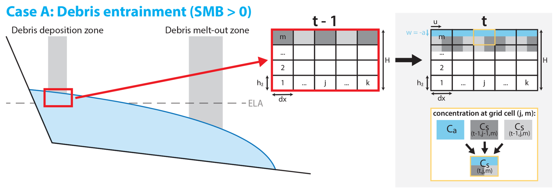
Figure 1 Implementation of debris entering the 2-dimensional grid as a concentration in the user-defined input area if in the accumulation area (mass balance > 0). The evolution of C_s, the debris concentration in the uppermost cell, at grid point j between time steps t−1 and t is defined in Eq. (7). C_a is the debris concentration in newly accumulated ice, computed from debris input rate d_in and surface mass balance a. C₀ is concentration in the debris-free layer advected along ice velocity u from upstream of the debris input area.

Debris melt-out d_out in the ablation area, a sink for debris concentration at the boundary of the englacial grid and a source for the debris thickness D, is given by:

$$\begin{array}{}\text{(8)}& d_{\mathrm{out}}=C_{\mathrm{s}}a/h_{\widehat{z}}.\end{array}$$

2.4 Terminal debris boundary condition

At the terminus, we follow Ferguson and Vieli (2021) and assume the surface debris to slide off the glacier at a terminal ice cliff of a critical height H^*, as expressed in Eq. (9) below. When ice thickness falls below this critical value, surface mass balance a is set equal to the debris-free mass balance $\stackrel{\mathrm{̃}}{a}$ over the fraction of the grid cell that is covered by the ice cliff. This approach avoids an infinite piling up of debris near the terminus where horizontal ice flow goes to zero in the SIA-approximation. It is supported by the observation of terminal ice cliffs typical at debris-covered glacier termini, in particular for currently retreating glaciers (Ferguson and Vieli, 2021).

$$\begin{array}{}\text{(9)}& a=\mathit{\{}\begin{array}{ll}\stackrel{\mathrm{̃}}{a}\frac{D_{\mathrm{0}}}{D_{\mathrm{0}}+D},& \text{where}H>H^{*}\\ \stackrel{\mathrm{̃}}{a},& \text{where}H\le H^{*}\end{array}.\end{array}$$

2.5 Numerical implementation

The basic numerical implementation of this model is described extensively in Ferguson and Vieli (2021) and complemented for the englacial tracking part in Ferguson (2022). In summary, the debris–ice system is resolved through the application of finite differences. The surface evolution of ice flow is discretized using forward differences and discretizations, whereas debris transport uses centered differences both on regular horizontal (dx=50 m) and vertical (m=40 layers) grids. To ensure numerical stability we ensure that the Courant-Friedrichs-Lewy (CFL) condition is satisfied (Courant et al., 1928). Special attention is also given to numerical diffusion in englacial debris transport, which is counteracted by implementing an anti-diffusion advection scheme in Smolarkiewicz (1983). Debris input and melt-out are computed through the boundary condition in the uppermost layer of the grid (Eq. 7 and 8).

2.6 Experimental setup

For comparability, we use a simple synthetic bed geometry similar to Ferguson and Vieli (2021) that represents a typical debris-covered glacier and is constant and gently sloped at 5.7° (or 100 m of elevation per km distance) for the main trunk of the glacier and has a steep (45°) headwall above (e.g., Fig. 2). The ELAs are generally chosen to be well below the headwall and with debris input in the accumulation area (but still below the headwall) as we are mainly interested in the case of englacial debris transport. Our narrow, constrained debris input area (e.g., Fig. 2a) with a usually temporally and spatially constant debris supply is based only on rough estimates for erosion rates from literature (Anderson and Anderson, 2016) and an implicit assumption of where debris would likely be deposited on the glacier.

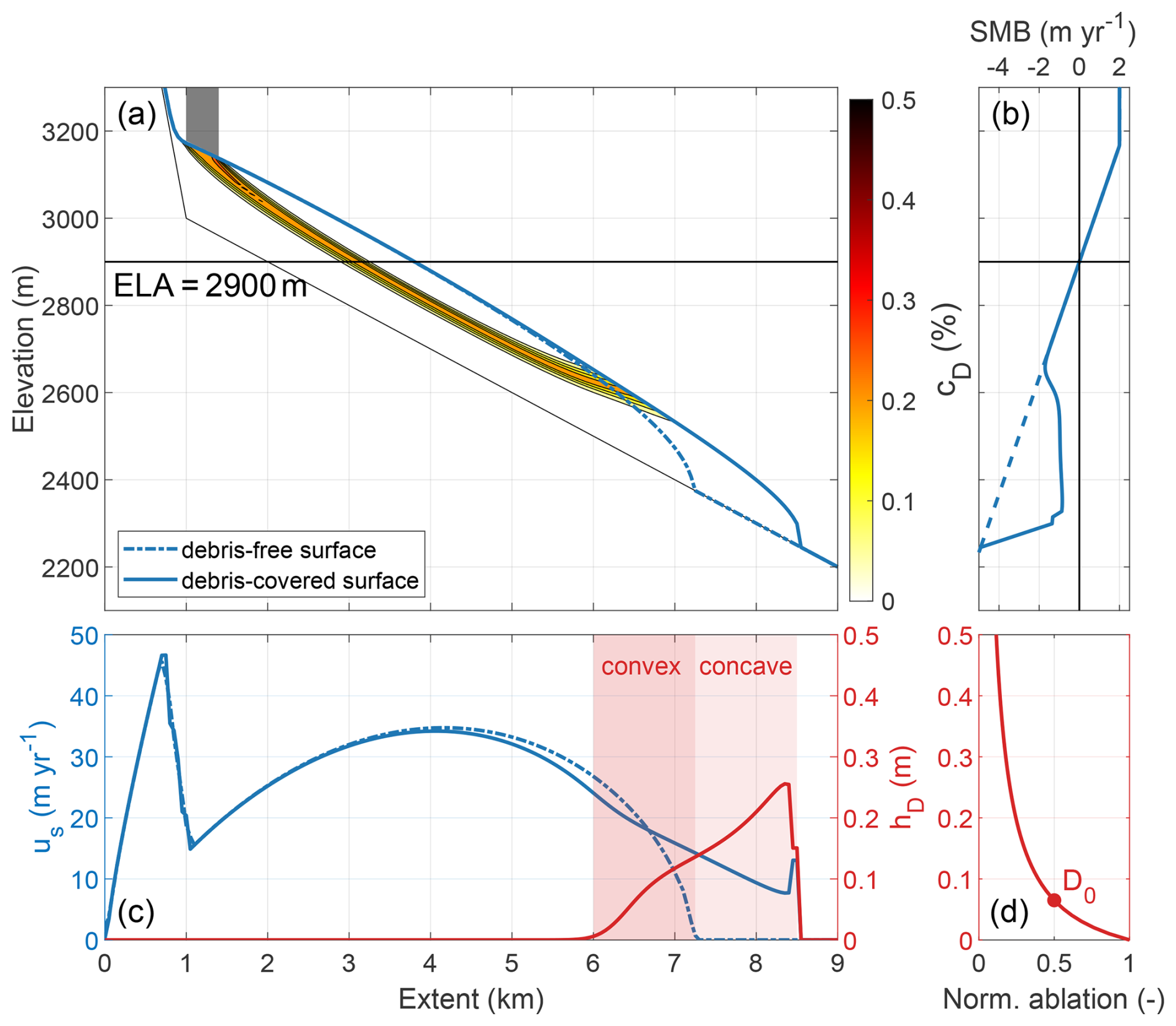
Figure 2 Experiment steady-1: (a) steady-state surface geometries for a debris-free and a debris-covered glacier with the same constant ELA at 2900 m (blue lines). For the debris-covered glacier, the gray area marks the 400 m wide debris input area with input rates of 4.5 mm a⁻¹, the colored areas within the glacier indicating the englacial debris concentrations in %. (b) Surface velocities of the debris-covered and debris-free glaciers (blue) and corresponding debris thickness h_D (red), where the light red areas mark convex-up and concave-up sections of the along-flow debris cover distribution.

In general, we first create a debris-covered glacier for a standard reference parameter set (Table 1), by building up a clean-ice glacier for a given ELA, then adding the debris in the debris input area and running it to a steady state. A steady state is reached when the glacier surface reaches an equilibrium (glacier-averaged $|\partial H/\partial t|<{\mathrm{10}}^{-\mathrm{3}}$ m yr⁻¹ for 100 years). If not stated differently this glacier geometry will then serve as the initial state for further experiments.

Table 1 Forcing variable ranges and reference model parameters for the numerical experiments.

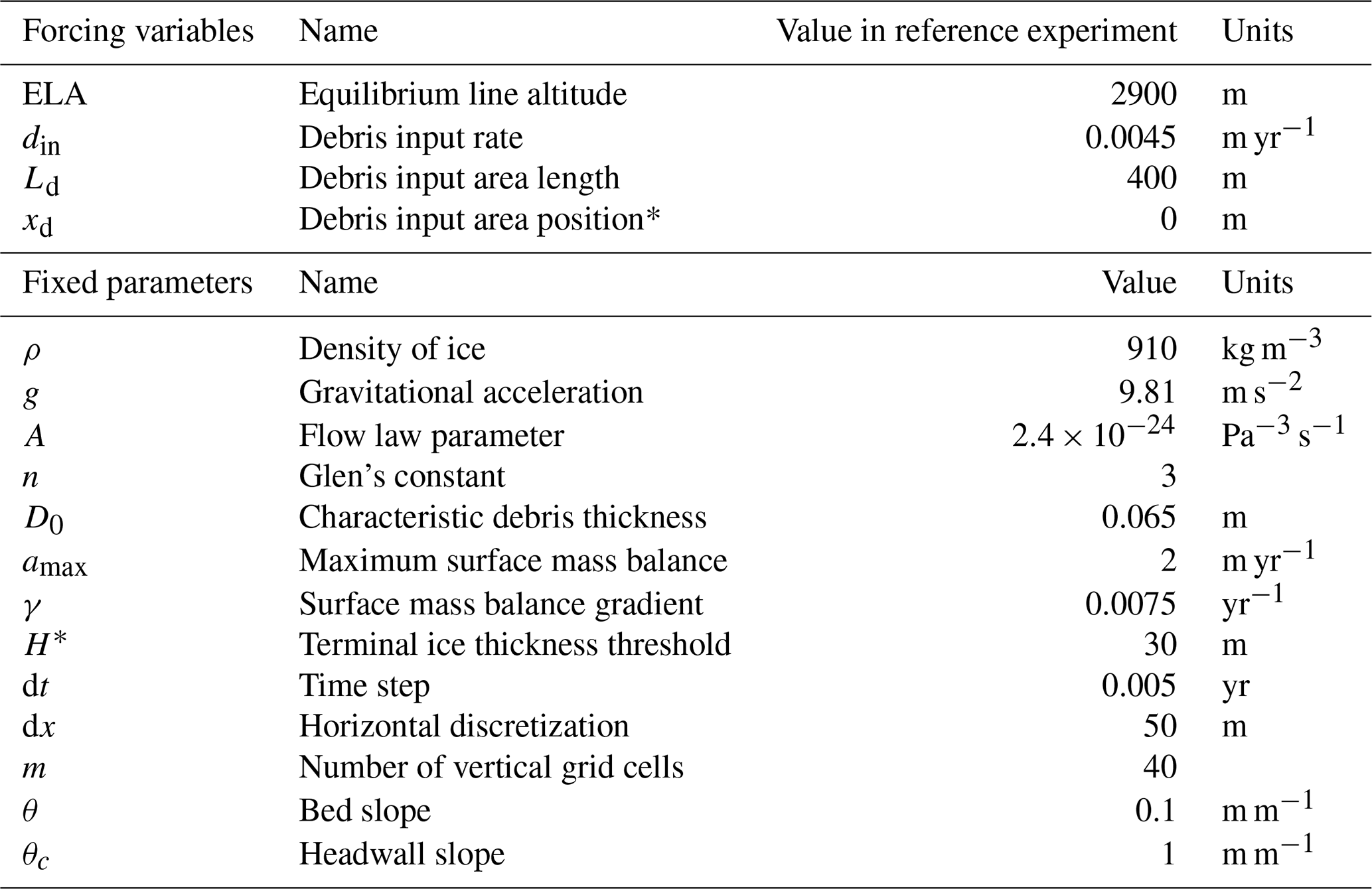
^* Relative to headwall slope break.

We perform a suite of modelling experiments, where we first consider steady-states (Sect. 3.1), mostly adapting and re-evaluating experiments conducted in previous studies (Anderson and Anderson, 2016, 2018; Ferguson, 2022). We then explore transient responses (from Sect. 3.3) to variable climates (labeled as clim-x experiments), introduce step-change perturbations and periodic fluctuations, and finally approach a realistic transient Alpine climate (Lüthi, 2014; Masson-Delmotte et al., 2021). Next, we consider variable debris inputs (labeled as deb-x; see Table 2). We quantify long-term glacier response times that are relevant for predicting the future state of debris-covered glaciers and the timing of their retreat. The considered time spans for these experiments are usually 3000 or 6000 years, which is rather long but necessary due to the expected slow adjustment timescales of debris-covered glaciers (Ferguson and Vieli, 2021). All experiments are conducted using the parameters provided in Table 1. An overview of all experiments and respective forcing variable ranges is given in Table 2. The parameter ranges are mostly extracted from the modelling literature (e.g., Anderson and Anderson, 2016; Ferguson, 2022). To further test and better understand the robustness of the model we undertook additional sensitivity and validation experiments related to model reversibility, debris mass conservation, characteristic debris thickness D₀, ice rheology and terminal ice cliff height. These results are presented in detail in Appendices C and D, but integrated in the discussion of the main model experiments where relevant. We avoid using parameter combinations and spin-up implementation in our general experiments that were found to cause issues with mass conservation and reversibility. For consistency across all experiments we define a reference model parameter set (Table 1) and vary only forcing variables, while other parameters are considered fixed and only explored in Appendix D.

Table 2 Overview of undertaken numerical experiments.

3 Modelling experiments and results

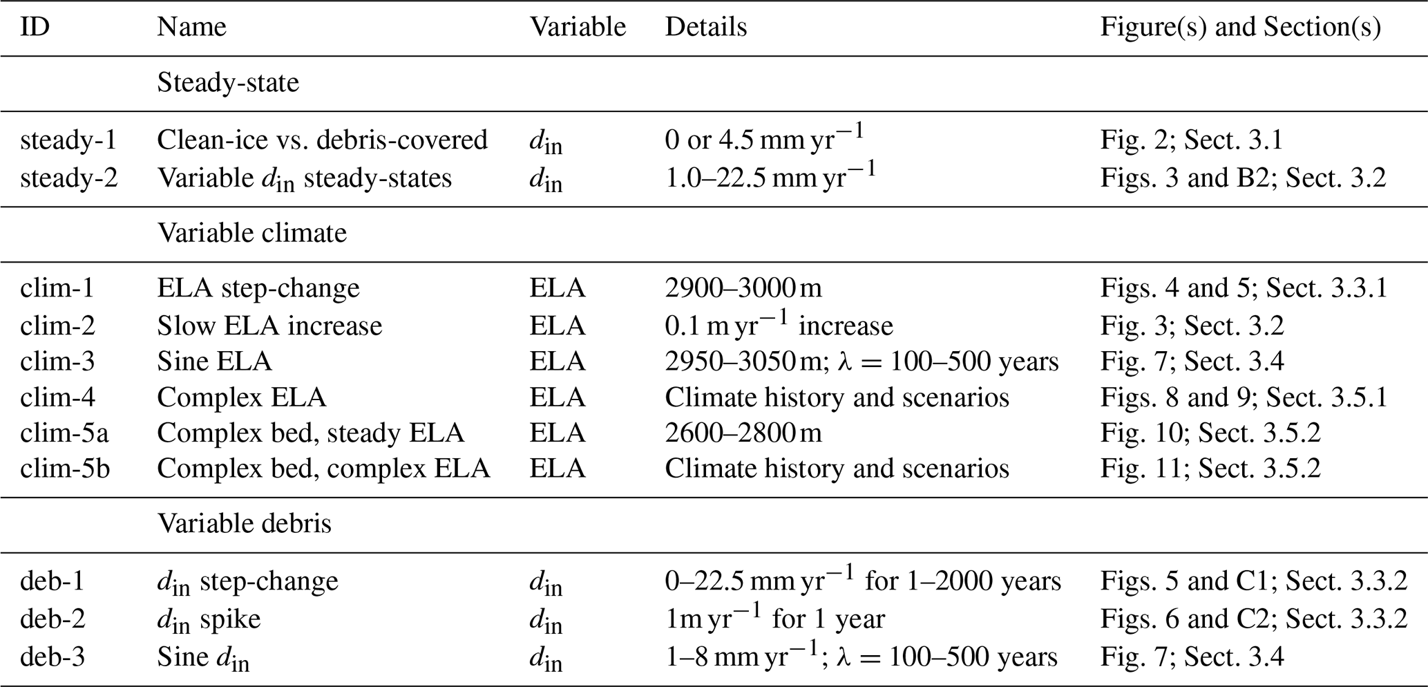
In this section we perform our main modelling experiments with a particular focus on the transient response of debris-covered glaciers to changes in debris input and climate. The experiments are structured along an order of increasing forcing complexity, where we first consider steady-states (Sect. 3.1) before moving on to simple transient responses (from Sect. 3.3), and finally exploring more realistic model forcing in Sect. 3.5.

3.1 Debris-covered glaciers in steady-state

In a first step, we explore various sets of constant forcing variables and their corresponding steady-state glacier geometries. From these stable states assess the impact of the inclusion of debris cover on the glacier geometry and debris thickness distribution in an otherwise constant set of forcing variables and parameters. To assess the relationship between a glacier and debris cover, we first compare steady-states of a debris-free glacier to the case where we add debris at a fixed rate and fixed location below the headwall (but above the ELA). In this configuration, debris reaches a depth of about 50 % of the ice column (Fig. 2a), resulting in extensive debris-free as well as debris-covered regions. As previous studies have shown (e.g., Anderson and Anderson, 2016), the general shape in surface geometry of the debris-covered glacier compared to the debris-free one is largely congruent (Fig. 2a). Only below the position where debris starts to emerge do the two surfaces start to diverge (at around 6 km). The debris-covered glacier produces a more elongated tongue sustained through the insulating effect of the debris. The along-glacier shape of the debris thickness is slightly convex-up in the melt-out area, transitioning to a concave-up shape near the terminus (Fig. 2b), as previously observed by Anderson and Anderson (2018). Note that the flattening of the surface in the debris melt out area can also be seen in the slight decrease in velocity there (between 4 and 7 km along the glacier).

In Appendix B2, we repeat experiments conducted by Anderson and Anderson (2016) comparing different debris input rates and positions. We come to the conclusion that, while debris cover leads to an elongated steady-state geometry, it only minimally affects up-glacier dynamics and shape. The length of a glacier is linearly proportional to the quantity of debris supply, even though the increase in the protective effect diminishes for thick debris. In terms of debris input location, its proximity to the ELA strongly influences total debris-covered area and length of the glacier.

3.2 Compensation of warming-induced melt by debris cover

Here, we directly put the ablation reduction effect of debris cover into perspective by comparing it to a (permanent) change in ELA, comparing debris-free and debris-covered glaciers by finding the ELAs where their size is equivalent. The concept of dELA (as established in Sect. 2.2) describes this comparison, relating steady-state debris-free ELA to a corresponding debris-covered ELA that both lead to a glacier equivalent in either volume or extent. Figure 3 shows this comparison for four debris-covered glaciers with different debris input rates d_in (1.0–22.5 mm yr⁻¹). Both volume- and extent-derived dELA show a linear relationship to d_in (Fig. 3a). We can infer from this that steady-state glacier size linearly scales with debris input, as is also apparent from Fig. B2a. The thin, elongated shape of debris-covered termini mean that dELA of extent is consistently about double that of the volume, meaning that an increase in debris input would affect glacier length much more strongly than ice volume. As equivalent debris-covered ELAs (colored lines in Fig. 3b) run parallel to debris-free ELA (black line), dELA, which is the latter subtracted from the former, remains mostly constant (independent of elevation) as long as the ELA is not in the vicinity of the headwall (around 3100 to 3200 m). To summarize, debris-induced glacier elongation is linearly dependent on debris input and independent of ELA.

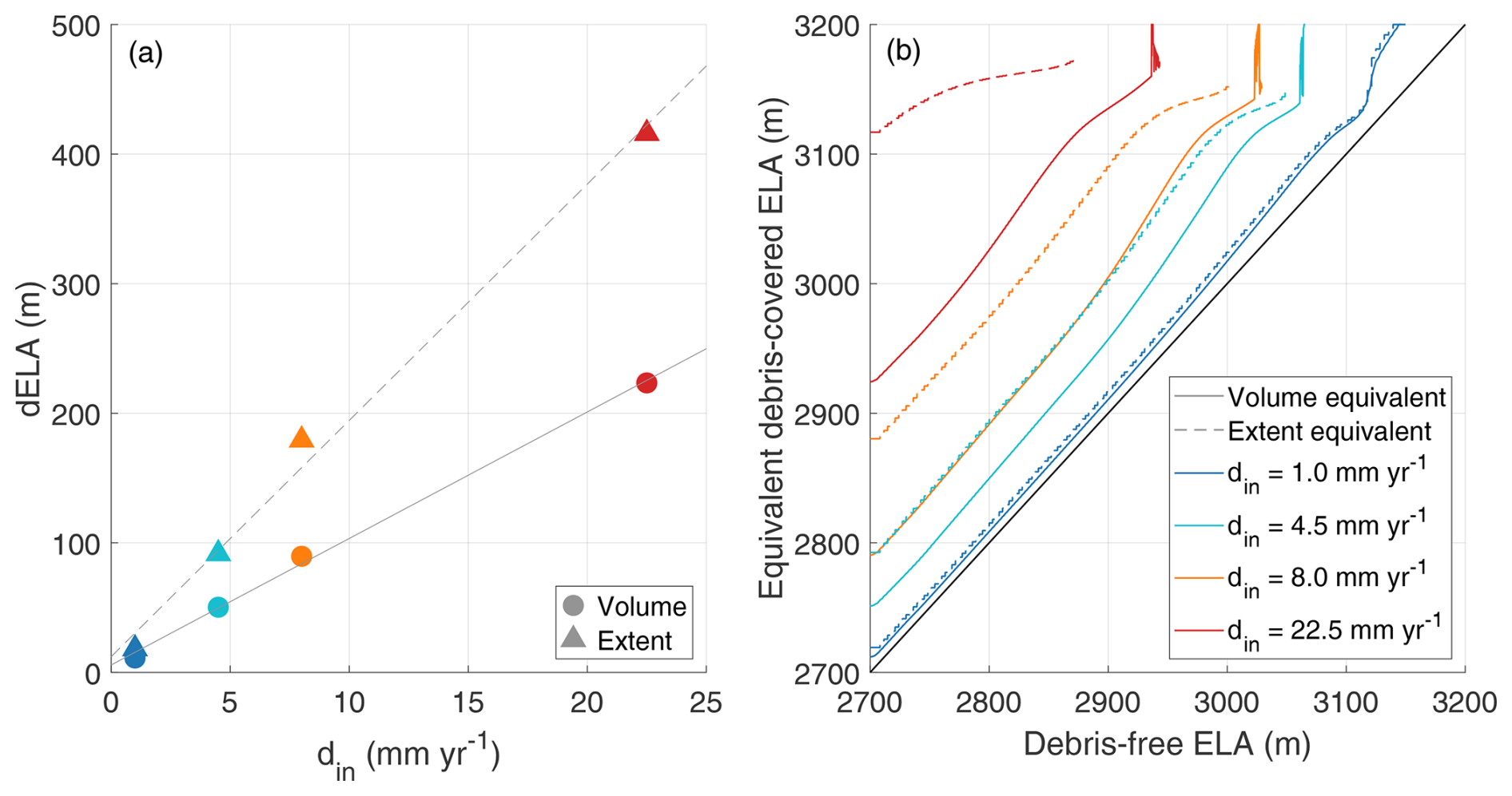
Figure 3 Experiments steady-2 and clim-2: (a) Relationship of steady-state debris input with dELA (dELA = equivalent debris-covered ELA − debris-free ELA, measured at 2700 m debris-free ELA) for volume and extent equivalent ELAs, showing a roughly linear relationship. (b) Debris-free ELA compared to debris-covered ELA, showing the debris-covered ELA required to result in a volume or extent equivalent to the debris-free case. Four cases are shown, with a debris input of 1.0 mm yr⁻¹ (blue), 4.5 mm yr⁻¹ (cyan), 8.0 mm yr⁻¹ (orange), and 22.5 mm yr⁻¹ (red).

3.3 Transient response to step-change forcing

Next, we apply simple transient forcings to the model and investigate the dynamic glacier response starting from the reference setup (Table 1). In a first set of experiments we repeat an experiment conducted in previous studies (e.g., Ferguson and Vieli, 2021) by applying an abrupt change in ELA (experiment clim-1) and, introducing a new experiment, a similar change in debris forcing (experiment deb-1), which we name as “step-change” in debris forcing. Over the long timescales of glacial response in experiments, an abrupt change in climate temperature as modelled here is quite similar to concurrent sub-century scale climate change. Still, climate conditions on real glaciers are subject to perpetual variations, never truly allowing a “steady-state”. This is why we later move on to periodic variation experiments (clim-3 and deb-3 in Sect. 3.4) and more stochastic (deb-2) and realistic (clim-4 and clim-5) variations (in Sect. 3.5).

3.3.1 Step-change in ELA

Figure 4 shows the response to a step-change warming (a and c) and cooling (b and d: experiments clim-1) by a change in ELA of 100 m (∼1 to 1.25 °C; Lüthi, 2014), in order to investigate differences in dynamic response between debris-covered and debris-free glaciers. In the advance experiment (ELA lowering; Fig. 4b and d), the length response of the debris-covered glacier is almost indistinguishable from the debris-free glacier response as demonstrated by the almost identical shape of the advance curves. The advance is accompanied by an initial decrease in total surface debris (Phase 4 in Fig. 4d/f) as the debris melt-out position moves down-glacier. Once this melt-out position is stabilized, surface debris increases (Phase 5) as the debris-covered tongue advances (Video Supplement 1).

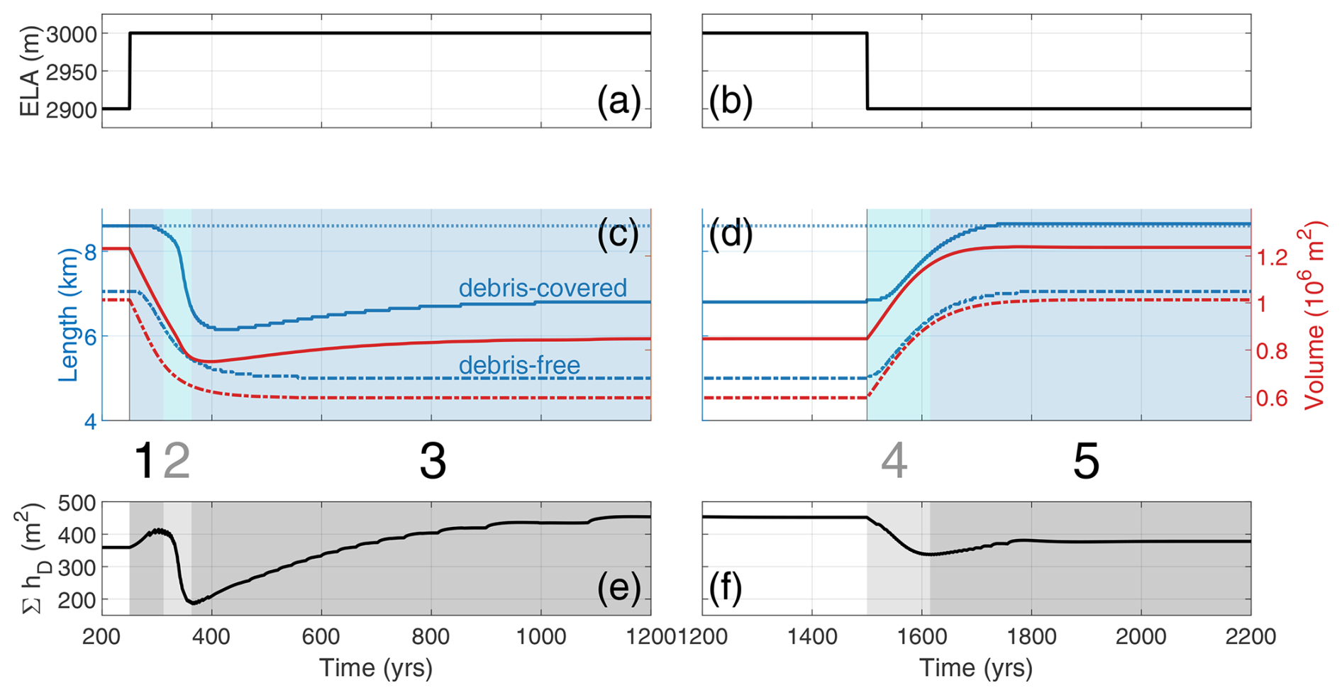
Figure 4 Experiment clim-1: ELA step-change experiments (Exp. clim-1) for (a) warming and (b) cooling with the related response (c, d) in debris-covered (blue solid line) and debris-free glacier length (blue dashed line) and glacier volume (corresponding red lines) and (e, f) total surface debris volume Σh_D. The shaded areas mark different phases (1–3 after warming, 4 and 5 after cooling) of length and debris cover response referred to in the text.

In the retreat case (Fig. 4a and c; increased ELA), the response of the debris-covered glacier, however, distinctly differs from the debris-free case. In a first phase (Phase 1 in Fig. 4c/e), the debris-free glacier starts retreating almost immediately as a result of increased mass loss and thinning (Fig. 4c), whereas the debris-covered glacier terminus remains and does not retreat for several decades, despite already rapidly losing mass. In Phase 1, it already starts accumulating more debris at the surface (Fig. 4e), due to enhanced debris melt-out and an expanding surface debris area (see increase of total debris by red line). In a second phase lasting a few decades (Phase 2), the debris-covered glacier abruptly retreats as the glacier tongue eventually thins away and collapses (blue solid line in Fig. 4c) and the terminal section with thick debris cover is now removed, hence the remaining total debris volume on the glacier surface strongly reduces (black line in Fig. 4e). In a third phase that lasts centuries (Phase 3), the glacier recovers slowly from its maximal retreated length position to a slightly more advanced new stable retreated state (Fig. 4c). During Phase 3, the supraglacial debris volume slowly builds up again to reach a total volume that is even higher than in the initial cold phase (Fig. 4e). This implies an inherent change of debris cover that comes with an abrupt change in ELA, given a fixed debris input rate and source.

Figure 5 summarizes the response in length and volume together with the corresponding e-folding response times. These e-folding response times quantify the time it takes for the glacier geometry to adjust by a fraction of $\mathrm{1}-\frac{\mathrm{1}}{e}$ (about 63 %) of change between the initial and final state after a step-change in forcing. Commonly, the response time refers to the adjustment in volume (Johannesson et al., 1989; Zekollari and Huybrechts, 2015) but the concept of e-folding time can also be applied to the length adjustment (Oerlemans, 2007). We find that for our experiment the response times of debris-free and debris-covered glaciers to a step-change in ELA do not drastically differ. Length response is generally a bit slower than volume response in all cases, but the onset of length retreat of the debris-covered glacier is strongly delayed (40 years), as previously observed by Ferguson and Vieli (2021). Nevertheless, the subsequent rapid retreat of the debris-covered glacier causes e-folding response time to be only 18 % slower than the debris-free response. The only exception is for the advance case, where the volume response is even shorter in the debris-covered case, which might be connected to the already more extended steady-state length before the advance. As mentioned above, the response to warming is also non-monotonic. The initial response in both length and volume first retreats beyond the final steady-state (Phase 2), then slowly re-advances to the final stable state (Phase 3). When we include this slow rebounding phase in the calculation of the response time, we obtain values that are several times higher than the classic e-folding response time for retreat (Fig. 5b and c) and can be attributed to the timescale of transporting the debris through the glacier before it melts out at the surface. Finally, note that after reaching the final steady-state (Fig. 4d), resetting the ELA forcing to the initial value of 2900 m as before the warming, the terminus does not exactly return to its initial position and equilibrates in a slightly more elongated state. This effect is specific for this experiment and is discussed in detail in Appendix C1.

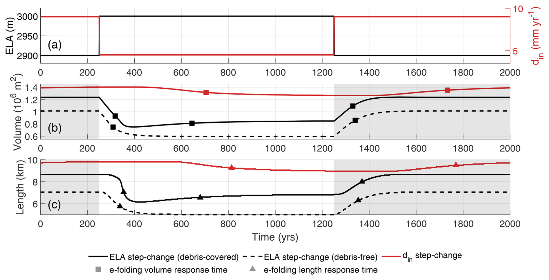
Figure 5 Experiments clim-1 and deb-1: Response times to a step-change in ELA (Exp. clim-1), for a debris-covered (black solid line) and a debris-free glacier (black dashed line), and to a step-change in debris input rate d_in (red solid line; Exp. deb-1): (a) forcing, (b) volume response and e-folding volume response times, and (c) length response and e-folding length response time. The symbols mark the time of reaching the response time (e-folding time) after the step-changes.

3.3.2 Step-change in debris input

We conduct a further step-change experiment where we vary the debris input rate instead of the ELA (Exp. deb-1), by decreasing d_in from 1 to 9 mm yr⁻¹ and back while always keeping the ELA fixed at 2900 m. Figures 5 and C1 show advance and retreat after an increase or decrease in debris input rate respectively. Comparing the debris step-change experiment to the climate forcing experiment (Fig. 5), we find highly contrasting qualitative response behavior. Both glacier volume and length show no reaction for about 300 years followed by very slow retreat or advance phases. Similarly, as in the slow rebounding Phase 3 in the ELA warming experiment, these highly delayed responses to debris input forcing are a result of the englacial transport times of the debris from input to melt-out. This transport of debris through the glacier and strongly delayed resurfacing on the glacier tongue is clearly visible in experiment deb-2, where brief (1 year long) spikes in debris input are deposited in the accumulation area every 1000 years (Fig. 6b). We can also observe the effect of these spike events in temporarily increasing both debris thickness and glacier extent for over a hundred years (Fig. 6c).

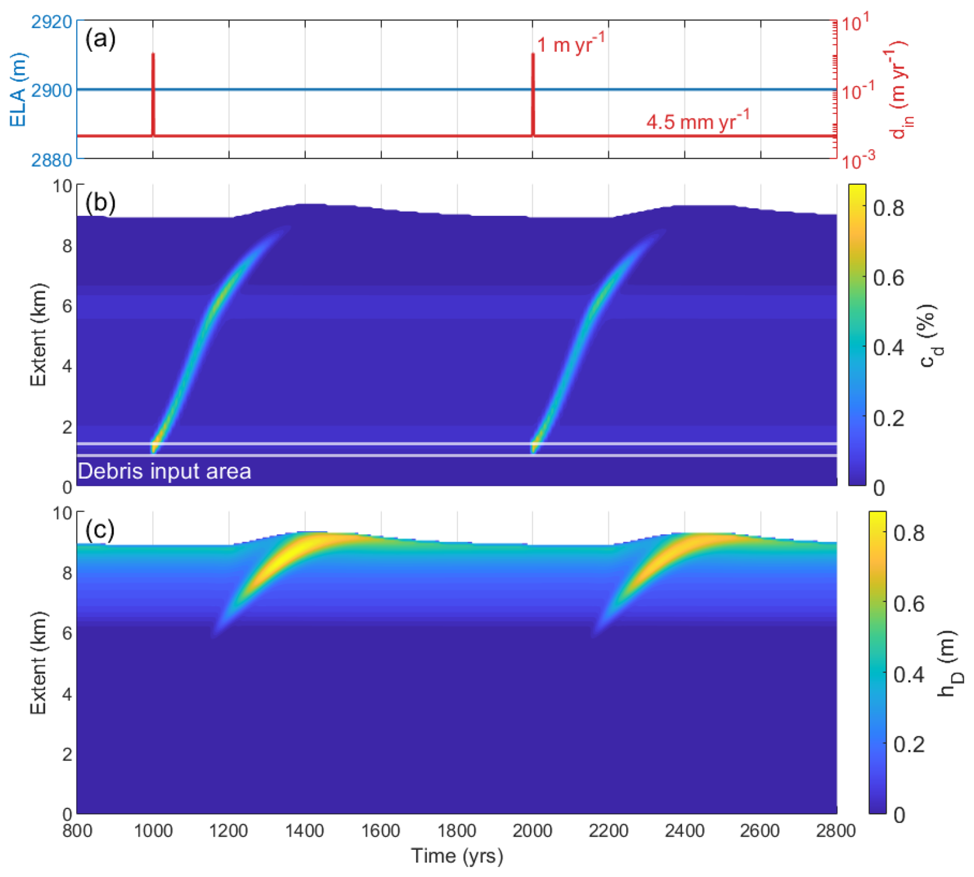
Figure 6 Experiment deb-2: Short-term debris input spike experiment (Exp. deb-2): (a) constant ELA and spike debris input rate forcing, (b) resulting depth-averaged englacial debris concentration over time and glacier extent, and (c) resulting debris cover thickness over time and glacier extent. During the spike event, 1 m of debris is deposited on the glacier over 1 year. In the intermediate periods the standard debris input rate of 4.5 mm yr⁻¹ is used.

Thus, beyond the generally slightly enhanced delayed response of debris-covered glaciers to climatic forcing, the additional delay when tracking englacial debris implies that a response to change in debris operates on a different, longer timescale than a response to climate. We observe a similarly long lag in Phase 3 (re-advance) in the debris-covered glacier response to warming (Figs. 4c and 5). Similarly to the ELA experiment, we notice that there is a slight discrepancy between the final steady-state and initial state after a first cycle of debris input step-change (increase followed by decrease; e.g., Fig. C1), which is further explored in Appendix C1.

3.4 Transient response to periodic debris and climate variations

In a next step of transient experiments, we examine how periodic variations in climate or debris input affect a debris-covered glacier. For this purpose we repeat an experiment from Ferguson (2022), periodically and separately vary the ELA with a sine function (amplitude = 100 m) and introduce a new experiment forcing a sine wave in debris input rate (amplitude = 7.0 mm yr⁻¹) around the respective reference values (ELA = 3000 m and d_in=4.5 mm yr⁻¹; Fig. 7). Additional periodically transient experiments can be found in Appendix B3. Generally, we observe that variations on timescales of several decades (Fig. 7a) do not substantially affect glacier geometry, in particular in length, as long as there is no long-term background trend in the forcing. This is particularly true for variations in debris input, which do not seem to have any impact on the glacier length and volume on timescales below 200 years. In this case, even though debris thickness upstream might vary substantially over time, the glacier terminus is, within the grid resolution, almost stable.

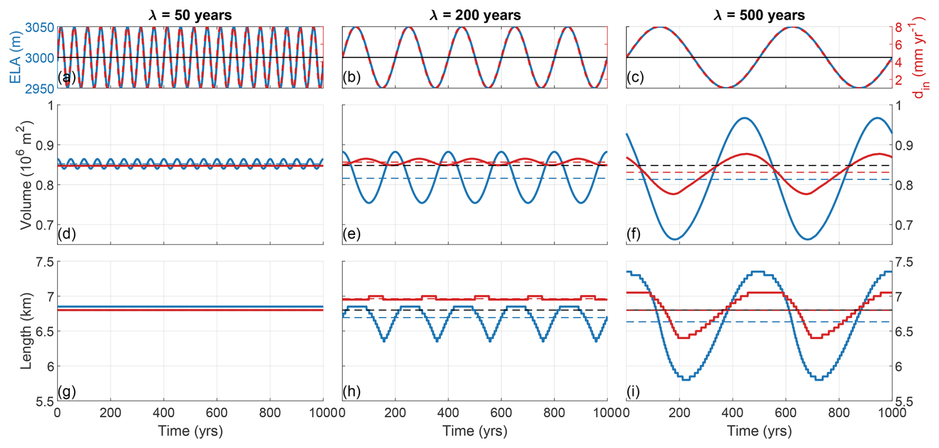
Figure 7 Experiments clim-3 and deb-3: Comparing glacier volume and length response to sine variations in climate (ELA, blue solid lines; Exp. clim-3) and debris input (d_in, red lines; Exp. deb-3) forcing with three different period lengths: (a, d, g) 50 years, (b, e, h) 200 years, and (c, f, i) 500 years. Dashed lines indicate volumes and lengths of a steady-state glacier (black) with the corresponding time-constant mean ELA and debris input rates, compared to mean volumes and lengths of the transient-state glaciers (blue and red lines).

Due to the effect of debris, the glacier geometry seems unresponsive to forcing fluctuations at timescales below a century and the glacier reaches a pseudo-steady-state. In contrast, for debris-free glaciers, the frequency of variations required to have a significant impact on the glacier also depends on the glacier's response time, which itself can be impacted by a variety of factors such as glacier size, slope, and ice temperature (Johannesson et al., 1989; Bahr et al., 1998). In terms of quantitative effect on the glacier, changes in ELA seem much more impactful than changes in debris input, at least under the conditions of our parameter ranges. For example, in Fig. 7, oscillating the ELA by just 100 m has a larger effect on the glacier than varying debris input rates between 1 and 8 mm yr⁻¹ (multiple times). A variation of 100 m roughly corresponds to 1 to 1.25 °C (Lüthi, 2014), which is reasonable for temperature variations in the Alps over the last millennium (Goosse et al., 2018).

3.5 Towards more realistic forcing

In this section, we aim to work towards more realistic debris-covered glacier behavior by exploring the effect of more complex climate forcing signals (Exp. clim-4) and bed topography (Exp. clim-5a/b) on a debris-covered glacier. While attributing the response to forcing might not be as direct as in the idealized cases above, these experiments include additional aspects such as noisy forcing signals in a warming world or more variable along-flow variations in flow speed and debris thickness from undulations in bed topography.

3.5.1 ELA history forcing

Our climate forcing curves for experiment clim-4 (Fig. 8a) are based on data from two publications: Lüthi (2014) for the past 2000 years until the year 2020, Masson-Delmotte et al. (2021) for the following 1000 years into the future. The Lüthi (2014) dataset reconstructs ELA history from alpine paleo-glacier variations over 2000 years until the year 2020. After 2020, we rely on temperature projections based on shared socioeconomic pathways (SSP). SSP1-1.9 (low emission), SSP2-4.5 (intermediate emission), and SSP5-8.5 (high emission) represent different scenarios of how global temperature may develop until the year 2090, based on projected changes in anthropogenic carbon emissions into the atmosphere. We use the best estimates for each scenario of temperature change until the 2081–2100 period (Masson-Delmotte et al., 2021) relative to the 1850–1900 reference period. We assume linear temperature increase between the years 2020 and 2090 (the middle of the 2081–2100 period), followed by steady temperatures. We convert temperatures to ELA by multiplying with a sensitivity factor of 90 m K⁻¹ (i.e. 90 m per degree temperature change) based on the estimate of 80–100 m K⁻¹ by Lüthi (2014). Finally, we add artificial decade-scale noise to the projected ELA curve (normally distributed, standard deviation matching the Lüthi, 2014 data). Note that the debris input area and rate are kept constant at 4.5 mm yr⁻¹. The chosen ELA history is not meant to be an accurate representation of real changes in climate or glacial response to it, but rather to provide representative temporal forcing patterns and trends in ELA for observed climates for the past millennia (medieval warm period, LIA cooling, decadal variations, future longer-term warming trends). Due to the observed long delays in response of debris-covered glaciers we start our forcing history at 1950 BCE (hereafter denoted as year 0).

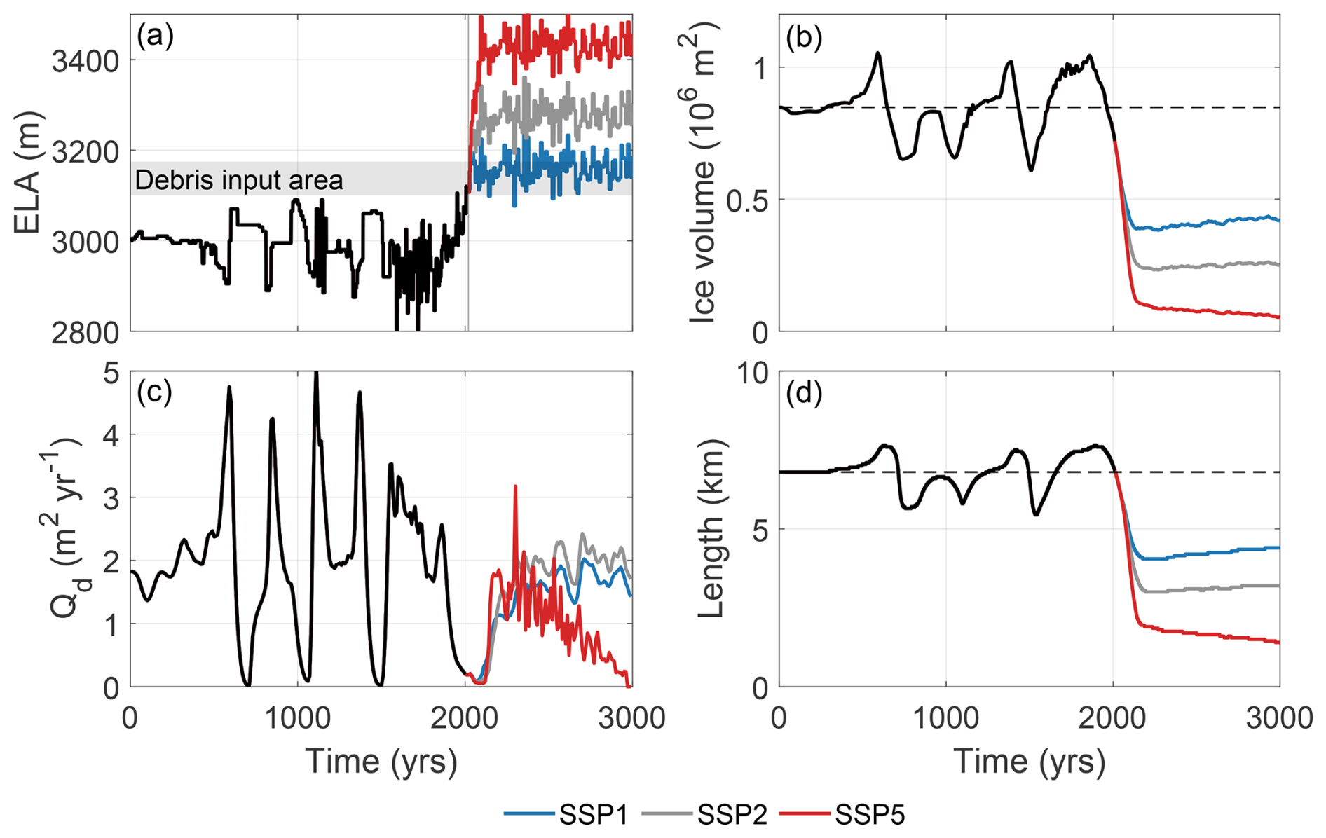
Figure 8 Experiment clim-4: Debris-covered transient response to complex climate forcing, based on a reconstructed climate history (Lüthi, 2014) and SSP1-1.9 to SSP5-8.5 climate scenarios (Masson-Delmotte et al., 2021) with synthetic short-term fluctuations: (a) ELA forcing, (b) volume response, (c) debris flux near terminus, and (d) length response.

Many of the observations made in previous experiments persist. Firstly and consistent with our earlier periodic forcing experiments, the short-term fluctuations in forcing (mostly from year 1500 onward) are filtered out in the volume and even more so in the length response (Fig. 8). Secondly, the retreat behavior during long warm or warming periods is similar to the step-warming case: a stagnating thinning tongue (Fig. 9c) followed by a rather abrupt retreat and ultimately slow re-advance through the build-up of a thick debris layer (Fig. 9b). However, we see that this re-advance and thick debris layer only appears when the ELA remains roughly constant over multiple centuries (e.g., in the years 0 to 500 and 2100 to 3000 in Fig. 9). During periods with high variability (decadal- to century-scales), the debris layers remain much thinner than during periods with near-constant climate (e.g., years 0 to 500, 2200 to 3000 in Fig. 9b). At the onset of warm periods and related stagnation and successive retreat, we observe that the flow speed and debris transport near the terminus are almost completely halted (Fig. 8c). Finally, the use of extreme climate scenarios (e.g., SSP5-8.5, the fossil-fueled society pathway from Masson-Delmotte et al., 2021) demonstrates well what happens when the ELA moves above the main body of the glacier and upstream of the debris deposition zone into the headwall. In this case, after the initial rapid retreat, the glacier keeps retreating extremely slowly, over hundreds of years. No rebound occurs here as the deposited debris always stays on the glacier surface and no delay from englacial debris transport occurs.

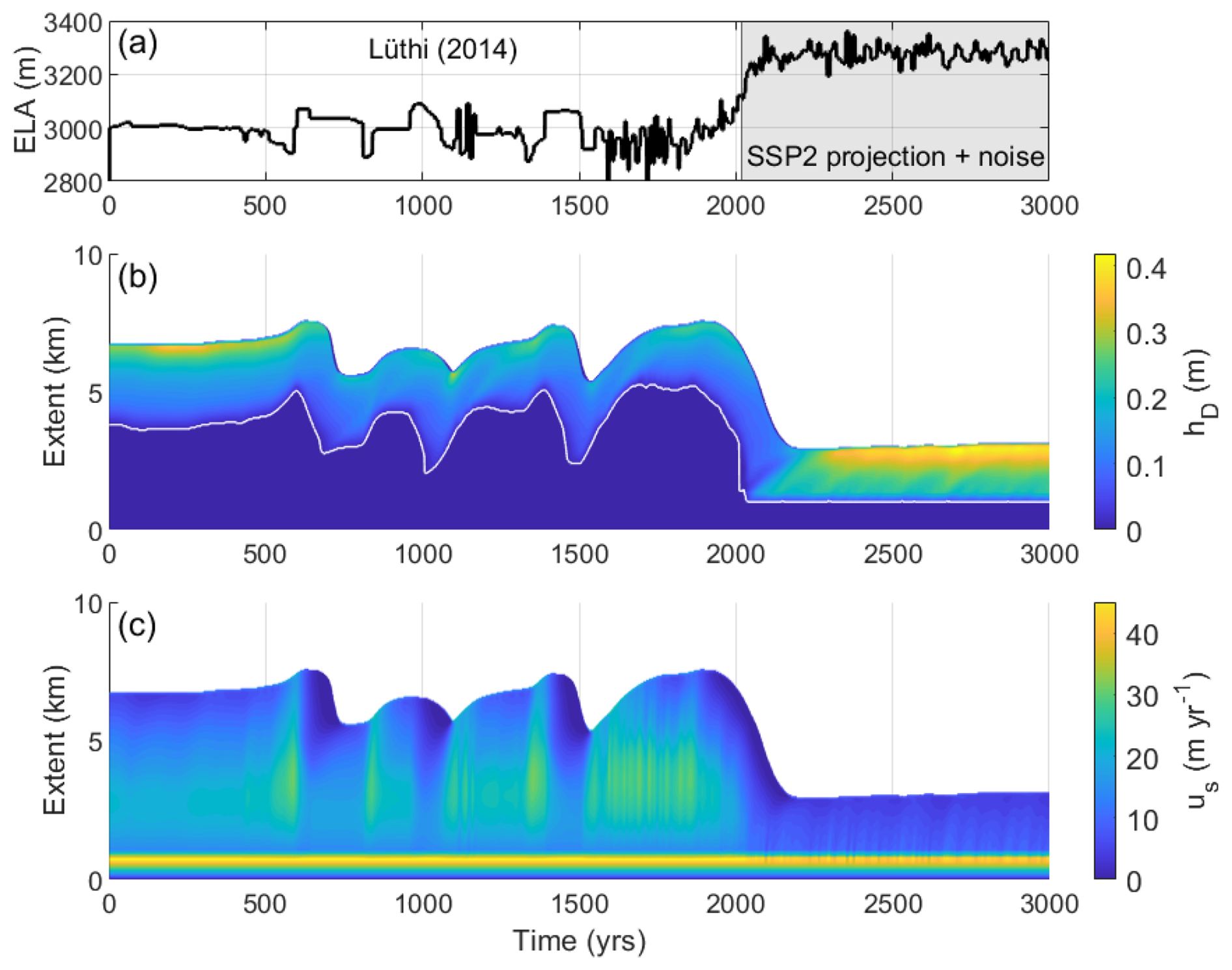
Figure 9 Experiment clim-4: Debris-covered transient response to complex climate forcing history: (a) ELA forcing derived from a reconstructed climate history (Lüthi, 2014) and SSP2-4.5 scenario (Masson-Delmotte et al., 2021) with superimposed synthetic short-term fluctuations, (b) debris cover thickness h_D response, and (c) surface velocity u_s response along the extent of the glacier. The white line in (b) marks the first grid point where debris thickness >0.01 m, i.e. where debris starts emerging.

3.5.2 Undulated bed topography

A last level of complexity is added when introducing a more realistic bed topography. As an arbitrary example for such bed undulations, we utilize an elevation profile along a flowline of Zmuttgletscher, Switzerland, derived from a helicopter-borne ground penetrating radar (GPR) survey (Langhammer et al., 2019; Mölg et al., 2020) with 50 m intervals. Figure 10 shows how this undulated bed and associated along-glacier variations in ice velocity (Fig. 11d) produce more variable debris cover patterns even in the initial steady state. This variability is more pronounced on a thinner glacier (i.e., ELA = 2800 m a.s.l.) or where bed roughness is increased (Fig. 10). Once we also apply the variable climate history (Fig. 11), an additional effect of complex topography (in direct comparison to the linear bed) appears: steep sections in the bed can cause detachment in phases of fast retreat, leading to stepped retreat and pockets of detached and stagnant (“dead”) ice (see the “overhanging” frontal margin around years 700 and 1450).

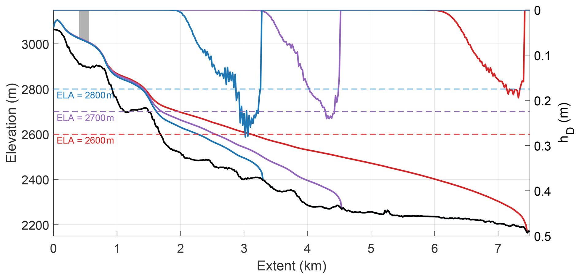
Figure 10 Experiment clim-5a: Influence of an undulated topography on steady-state glacier geometry: three steady-state glaciers (at ELAs of 2600, 2700, and 2800 m a.s.l.) and corresponding debris cover thickness (inverted scale, 0 at the top) on a bed topography adapted from Zmuttgletscher, Switzerland.

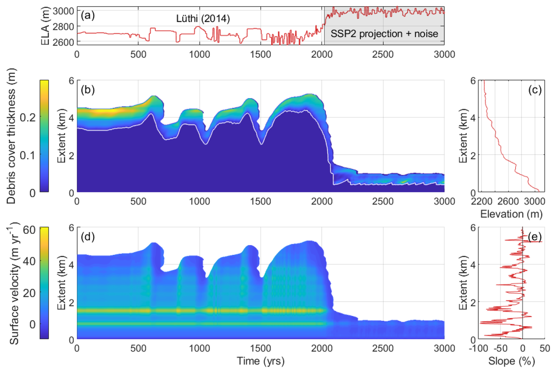
Figure 11 Experiment clim-5b: Debris-covered transient response to complex climate forcing on an undulated bed topography: (a) ELA forcing derived from reconstructed climate history (Lüthi, 2014), SSP2-4.5 scenario (Masson-Delmotte et al., 2021), and adjusted to produce a realistically sized glacier, (b) debris cover thickness response, (c) along-glacier bed elevation, (d) surface velocity response over the extent of the glacier on a Zmuttgletscher-like bed topography (Fig. 10), and (e) along-glacier bed slope. The white line in (b) marks the first grid point where debris thickness >0.01 m, i.e. where debris starts emerging.

4 Discussion

We have presented a model that couples ice flow to en- and supraglacial debris transport and explored related feedbacks in various forcing setups ranging from simple stable states to complex transient responses. Here, we aim to discuss these findings to gain a better understanding of the debris–glacier system in a transient setting.

4.1 Response to transient climate

In our transient climate forcing experiments (Exp. clim-1 to clim-5) we compare debris-free and debris-covered response in retreat and advance. Similar experiments were already conducted in Ferguson and Vieli (2021) with a simpler version of the model that does not include heterogeneous englacial debris transport. They also observe a delayed retreat response to warming connected to thinning behavior. Here, we characterize the transient debris-covered glacier response when including englacial debris-transport.

After warming, a debris-free glacier instantly starts both retreating and thinning (Fig. 4) because mass balance decreases, roughly linearly, towards the terminus (Fig. B3b), causing the lowest parts of the glacier to melt fastest. Conversely, debris cover thickness of a debris-covered glacier increases towards the terminus and ablation is suppressed there (e.g., Figs. C3b and B3c), leading to a flat or even inverse mass balance gradient (Anderson and Anderson, 2016; Ferguson and Vieli, 2021; Fig. B3b) and a stagnant terminus position, which have both been observed on real glaciers (Nakawo et al., 1999; Benn and Lehmkuhl, 2000; Benn et al., 2012; Thompson et al., 2016; Ragettli et al., 2016; Rounce et al., 2018; Mölg et al., 2019). One direct consequence of this flat mass balance gradient is the tendency of debris-covered glaciers to exhibit stagnation and thinning along the ablation area rather than terminal retreat in the first few decades of warming (Banerjee and Shankar, 2013; Ferguson and Vieli, 2021).

After this stagnating and thinning phase under warming (Phase 1), the debris-covered glacier abruptly retreats (Phase 2), accompanied by the loss of large parts of the supraglacial cover within decades (Fig. 4). During this period, debris flux is temporarily decreased in the ablation area (e.g., Fig. C3c), which has implications on studies relying on debris flux or other transport metrics to infer debris supply rates (McCarthy et al., 2022). As the glacier completes its dynamic adjustment to the change in climate, retreat comes to a halt. Subsequently, a slow process of debris cover recovery and subsequent re-advance begins (Phase 3), a behavior that has only recently been observed in a similar modelling approach (Verhaegen and Huybrechts, 2026). Debris cover rebounds for two distinct reasons: firstly, the now shorter englacial trajectory (further discussed in Sect. 4.4.1) leads to melt-out of debris further up-glacier. Secondly, ice mass turnover is reduced under the new warmer conditions, while the debris supply remains constant. This change in debris to ice ratio manifests in higher debris concentrations that only lead to a noticeable change in debris thickness after a lag period of englacial transport (Video Supplement 1), further discussed in Sect. 4.3). As the higher debris concentration reaches the ablation area and melts out, debris flux approaches its balanced quantity again (e.g., Fig. C3c), corresponding to the supply rate up-glacier. In the new warmer steady-state, the lower velocities counter-intuitively lead to higher total amounts of supraglacial debris in steady-state, even after retreat. However, this recovery takes hundreds of years, meaning, it is difficult to show or validate this newly discovered effect in experiments or observations under a climate varying on shorter timescales.

This is explored in the experiments (clim-4) applying a more complex climate with large variability on the scale of multiple decades to single centuries (Figs. 9b and 7c). Under such forcing, debris cover is regularly removed in phases of sustained warming and hence retreat (centuries), and by the onset of debris cover recovery, the climate is in most cases already changing (cooling) again, leading to thinner debris cover compared to an averaged constant climate. This leads us to the conclusion that long-term climate variability with phases of prolonged warming overall suppresses the formation of thick supraglacial debris layers that would be possible in steady-state or pseudo-steady-state climates. Ferguson and Vieli (2021) observed the opposite effect in their century-scale random climate experiment when using a homogeneous englacial debris concentration. This may be due to differences in experimental setup but could also indicate that incorporating depth-resolved englacial transport has a significant influence on the transient response.

During longer warm periods, debris transport near the terminus is almost completely halted (Fig. 8c) due to stagnation in ice flow. This leads to the debris layer not being transported off-glacier and only increasing in thickness through more debris melt-out while the ice is thinning. Dynamically stagnant tongues have been observed on many debris-covered glaciers (e.g., Thompson et al., 2016), but here we show new implications on temporal variations in debris transport and export from the glacier. Conversely, cooling leads to immediate acceleration of the ice (Fig. 9c) and therefore much faster debris transport, accompanied by instantaneous re-burial of any surface debris that is now above the ELA (advance of zero debris thickness line in Fig. 9b). The use of extreme scenarios (e.g., SSP5-8.5) illustrates the impact from an ELA moving above the main body of the glacier and behind the deposition area into the headwall. In this case the long-term re-advance trend vanishes as the ablation area of the glacier is no longer supplied with englacial debris (Fig. 8). This switch in long-term response is driven by the ELA crossing a threshold which is likely related to the location of debris input or, in a natural system, by crossing the foot of the headwall. This configuration of ELA and debris source in a model, combined with an avalanching mechanism, might also be able to represent rock glaciers (Anderson et al., 2018).

Further sensitivity experiments (see Appendix D) show that the general findings in transient behavior are robust and qualitatively indistinguishable to deviations in Glen's flow law parameter A (Fig. D1). Variations in the Østrem curve (parameter D₀) (Fig. D2) show a stronger impact on warming response. Specifically, a higher value of D₀ (weaker effect of debris on ablation) leads to faster, but less abrupt retreat and a less pronounced rebound, essentially exhibiting retreat more similar to debris-free glaciers.

The linear relationship between debris input and dELA described in Sect. 3.2 (Fig. 3a) suggests that an increase in debris input can compensate linearly for a warmer climate. Anderson and Anderson (2016) describe a similar relationship, but related steady-state glacier size to debris flux. However, in a transient state, debris flux is a product of debris input and ice dynamics. A dynamically induced increase in debris flux would actually lead to a more efficient evacuation of debris, causing thinner debris thicknesses and decreasing the protective effect of debris. Therefore, we argue that using absolute debris input in this context is more appropriate, as it disentangles observations from ice dynamics influence. The observation that dELA is independent of ELA (Fig. 3b) means that a fixed debris input will compensate the same ELA difference at any elevation, given a flat bed topography and an ELA-independent debris input rate.

4.2 Response to transient debris input

In our experiments with transient debris forcing (Exp. deb-1 to deb-2) we are able to characterize glacier response to a variable debris source. While past approaches assumed debris supply to be steady in space and time (Anderson and Anderson, 2016; Ferguson, 2022), the stochastic nature of gravitational processes and potential feedbacks with deglaciation (Banerjee and Wani, 2018; Hartmeyer et al., 2020) motivate our examination of spatially and temporally transient debris input. As described in Sect. 3.3.2, the response to changes in debris input often operates on a longer timescale than to changes in climate (Fig. 5). This is mainly a result of the required time of englacial debris transport from the source to the melt-out area, as nicely visible in Fig. 6b. Consequently, this “debris advection response time” highly depends on the position of the source in relation to the ELA. Long englacial pathways in a system where debris is added to the glacier high above the ELA lead to a slow response, both because of increased transport distance and decreased ice velocity in the lower parts of the ice column. Of course, the dynamic state of the glacier (mass turnover) is also relevant in a general sense, as a highly dynamic (e.g., fast flowing or advancing) glacier responds more quickly than a stagnant glacier.

Periodic (Exp. deb-3; Fig. 7) and random short-term (10 years) variations (Video Supplement 2) show that variability in debris input, in the absence of any longer-term trend, barely affects the glacier length evolution even on a century timescale. This shows that the debris-covered glacier system is insensitive to short-term fluctuations in debris input, unless the debris input occurs onto the ablation area or an isolated event several orders of magnitude larger than the long-term mean occurs (Fig. 6). Note that in the latter, depending on the englacial trajectory, the length-response can be delayed by several centuries (Vacco et al., 2010). At longer timescales (500 year wavelength), the response exhibits a phase shift of half a period, leading to a seemingly inverse relationship between debris input and glacier volume. This strongly supports the notion that recent changes in debris supply to the accumulation area are not readily apparent in observable variations of down-glacier debris cover patterns, thereby contributing to the complexity of the debris-covered glacier response. Approaches to infer long-term debris supply rates from debris cover (e.g., McCarthy et al., 2022) might profit from this smoothing process that should roughly average supply rates over several centuries.

4.3 The role of debris dynamics in the debris-covered glacier response

As illustrated in Sects. 3.3 and 4.2, we find that responses of debris-covered glaciers operate on multiple interfering timescales. While delayed retreat has been described in earlier studies (Ferguson and Vieli, 2021; Ferguson, 2022), we disentangle the complex response into tangible process interactions between debris transport and glacier mass balance. Post-warming volume loss (Figs. 4 or 5) shows that changes in ELA impact surface mass balance instantly, whereas any change to debris input in the accumulation area is transported englacially and can only take effect after it emerges at the surface in the ablation area. The time the debris cover thickness takes to fully adjust to a change in ELA during the post-retreat rebound phase is similarly long as the response to a change in debris input. It is also a direct consequence of englacial transport of newly higher debris concentrations. This concentration increase is a result of lowered ice accumulation in a warmer climate while absolute debris input remains constant (further explored in Sect. 4.4.1). Consequently, any change in debris concentration in the input area requires centuries to affect the glacier, irrespective of the underlying cause, whether it pertains to variations in debris input or ice accumulation. The duration of this lag is dependent on debris supply amount and most importantly debris input location relative to the ELA. This advection timescale becomes increasingly relevant when debris is deposited on the glacier in the accumulation area with increasing distance to the ELA. Further, the relative importance of the debris advection lag depends on ice dynamics, or more simply on glacier size. While increased ice velocities in larger glaciers lead to accelerated debris advection, small glaciers may have lower mass turnover, but generally shorter debris transport paths. As these effects counteract each other, the constellation of debris input area and ELA, given by local conditions, is much more relevant to response times. Assuming homogeneous debris concentrations (Rowan et al., 2015; Ferguson and Vieli, 2021) or positioning the debris supply at the margins (Margirier et al., 2025) risks over- or underestimation of the resulting debris cover, respectively.

The lag related to englacial transport further contributes to the attenuation of any debris input signal when observing debris cover. For example, a measured increase in debris concentration can either originate from increased debris supply or decreased ice accumulation at the time of formation. As such, this equifinality contributes to the complexity of inverting from debris cover thickness distribution to past debris input rates or historic climate states. In addition, once the debris has reached the surface in the ablation area, debris redistribution processes (Kirkbride and Deline, 2013; Moore, 2018; Bartlett et al., 2021; Ferguson, 2022) can smooth out or create new variations in along- and across-glacier debris distribution. For natural glacier systems with multiple debris sources that are variable in amount and position, have a sporadic record of debris cover, a variable climate history, and debris re-distribution such reconstructions become ambiguous if not impossible.

Reflecting on debris thickness measurement strategies, we can conclude that more extensive records of current debris cover might only marginally improve estimates of past debris input or climate. The long timescales involved in debris transport, as well as the fact that any measurement on debris-covered glaciers is constrained to our current period of warming, lead to an inherent observational bias (Ferguson and Vieli, 2021). Our modelling experiments enable us to evolve debris-covered glaciers in any climatic setting and over long timescales. Our results show that the relative positions of debris source and ELA are highly relevant to the extent of debris cover that influences glacier volume and extent. Within the debris-covered area, small-scale variations can rarely be traced back to a single source.

4.4 Transient debris-climate feedbacks

We have presented a multitude of transient experiments on a modelled debris-covered glacier, where we made observations about feedbacks in the system related to debris. Here we aim to discuss these feedbacks and the glacier system states resulting from them.

4.4.1 Englacial trajectory feedback

We have observed that a shift to a warmer climate leads to more debris being at the surface than in a cooler state (Fig. 4) if debris input occurs in the accumulation area. We can identify several processes leading to this debris cover increase.

Firstly, englacial trajectories are shortened as warming moves the ELA closer to the input area, similarly to when we move the position of the debris input area. This means debris spends a larger portion of its transport path on the glacier surface instead of englacially, decreasing mass balance. While the initial expansion of debris cover (increase in total debris in Fig. 4e) can be attributed to melt-out of pre-existing englacial debris within the ice as the glacier surface lowers, the permanent up-glacier shift of the debris cover is a consequence of this reduction in englacial path length (Video Supplement 1). The opposite effect applies to a glacier where debris is deposited onto the ablation area: warming causes the ELA to move away from the input area, causing a larger area above the debris input area (in the ablation area) to be debris-free, which increases melt. During intense and prolonged warming, a glacier might transition from depositing debris onto the accumulation area to depositing directly to the surface in the ablation area. We conclude that the shorter the distance between debris input area and ELA, the larger the debris-covered area and, consequently, the stronger the protective effect. Anderson and Anderson (2016) have previously described this relationship in their approach, further tying maximum debris cover extent to the proximity of debris input to maximum ice flux (at the ELA). This certainly holds true in steady-state but not in transient conditions, as ice and debris dynamics have different response times.

Secondly, ice velocities are lower for a thinner, shorter glacier corresponding to a warmer state. To satisfy debris mass conservation in the long-term, debris needs to be exported from source (debris input area) to sink (terminus) at a constant rate. For a glacier in balance, debris flux is constant along the entire glacier in a steady-state, which results in thicker debris in a warmer state. This effect applies independent of the relative position of the debris input area, as it entirely depends on changes in velocity.

Thirdly, as the system transitions towards a new equilibrium after warming, debris concentrations in the debris input area increase immediately. Englacial transport leads to a lag in response to this increase (see Sect. 4.3) that depends on the new relative position of the debris input area and ELA. After englacial transport and melt-out, the increased concentrations lead to further increase in debris thickness.

We summarize that, irrespective of whether local mass balance is positive or negative in the debris input area, the relative position of debris input to the ELA is highly relevant to the ablation reduction effect of debris in the ablation area, which increases as the two get closer. While warming leads to an increase in local debris thickness in all cases, expansion of the debris-covered area is limited to glaciers with debris input onto the accumulation area. Debris supply to the ablation area from unstable moraines, rockfall, or avalanching (van Woerkom et al., 2019; Stewart et al., 2025), where subsequent debris transport is exclusively supraglacial, may substantially contribute debris to the surface and lead to overestimation of expansion potential (Herreid and Pellicciotti, 2020).

4.4.2 Topography feedback

Basal topography strongly impacts glacier geometry (surface slope and ice thickness), especially for debris-covered glaciers. Slopes are usually steeper where surface debris is absent (in the accumulation area) and flatter where it is present (Sect. 3.5). Due to the inversely proportional melt reduction effect from debris thickness, steep topographic steps lead to enhanced melt-out of debris, which is rapidly propagated into the flat parts. There, the combined effect of flat terrain and debris-reduced ablation can further exacerbate the formation of elongated, low-velocity tongues on the flat valley floor.

Under a transient forcing, a more realistic, undulated bed topography based on a real glacier bed (Exp. clim-5; Figs. 10 and 11) can cause additional effects: (i) during a warming phase, the flat debris-covered parts with a concave bed can detach (Pellicciotti et al., 2015; Rippin et al., 2020; Rowan et al., 2021) from the steep sections just upstream, as melt rates are, due to the thinner debris, much higher there and the ice is already thin (compare Fig. 11 to Fig. 9), (ii) the concave shape of the bed favors elongated glacier shapes where small differences in ELA have a larger impact on the glacier. This means both more mass gain in advance and more mass loss in retreat, but favoring the elongated state because of the asymmetry between instant advance and delayed retreat discussed in Sect. 3.3.1.

4.5 Limitations

While our implementation of debris input and transport is close to achieving consistent debris mass conservation independent of climate, it still fails under certain circumstances. When debris is deposited too close to the ELA (Appendix C2) the model systematically underestimates debris cover. Consequently, the model is not fit for all combinations of climate and debris inputs. However, we have designed our experiments to minimize the impact of this inconsistency by avoiding parameter ranges where results are unreliable, thoroughly investigating issues, and focusing on relative results. This approach substantiates our confidence in the robustness of the results obtained.

A second intrinsic model issue is an inconsistency related to model spin-up. Depending on if a desired initial state is spun up from a less (e.g., debris-free) or more debris-covered state, terminus position will vary by a few grid points (Fig. C1; Appendix C1). The same issue leads to minor discrepancies between terminus positions before and after a phase of warming or increased debris supply. As all our model runs are spun up identically from a debris-free state (Fig. B1), we do not expect this to affect our results strongly. The issue is most likely connected to the implementation of the terminal boundary condition and is discussed in more detail in Appendix C1.

While we tested our approach on synthetic geometries and forcings, applying it to a specific real glacier would require the following inputs: a flowline bed topography, a climate timeseries, and some information about debris input locations. Further, our sensitivity analysis shows that the ablation reduction effect of debris cover is sensitive to D₀, for which a wide range of values is found in literature (Fontrodona-Bach et al., 2025), both quantitatively and in terms of transient behavior. For this reason, we believe constraining D₀ for individual glaciers is important to understanding their current and future behavior through modelling.

A further major assumption that might impact transient behavior concerns the boundary condition at the glacier terminus. There, we assume the presence of a terminal ice cliff, as in Ferguson and Vieli (2021). Our implementation is a crude approximation of real terminal ice cliffs as observed at some debris-covered glaciers (Nainwal et al., 2016; Mölg et al., 2019). Nevertheless, terminal morphology varies strongly between debris-covered glaciers (Rowan et al., 2015) and is not completely understood, forcing us to assume terminal conditions. These conditions affect the steady-state extent of the glacier (Fig. C4), but the transient response remains largely unaffected. For application to real glaciers, terminus conditions should be adapted to observed terminal conditions.

With respect to model forcing, specifically debris input, some studies suggest that warming may cause increased paraglacial rockfall activity, either directly from an increase in frost-cracking (Banerjee and Wani, 2018) or indirectly through deglaciation of rockwalls and the onset of weathering following surface exposure (Hartmeyer et al., 2020). Under this assumption, increased debris supply might actually help mitigate warming-induced retreat. Future approaches could constrain debris supply position by relying more on records of rockfall deposits or relating debris supply spatially to surface properties such as headwall slope or temperature (Scherler and Egholm, 2020). Additionally, models should also be improved by parametrizing surface processes such as debris re-distribution (Moore, 2018; Westoby et al., 2020), supraglacial-englacial debris exchange processes (Mayer and Licciulli, 2021), a more physically based surface energy balance model (Pellicciotti et al., 2026), the formation and impact of ice cliffs, or the formation of terminal ice cliffs and conduit collapses. A more complete record of research directions has been compiled by Nicholson et al. (2021).

5 Conclusions

We present a glacier flow-model that explicitly tracks englacial debris transport and advances previous approaches by enabling temporally and spatially varying debris supply, which is newly implemented entirely independent of climate forcing. This allows direct comparison between debris supply rates and observed downstream debris concentrations and thickness patterns. While some results may depend on model design choices, we explore the parameter space, assess the numerical robustness, and show the capabilities and limitations of this model. In a second step, we exploit these new capabilities by conducting a set of experiments to make some general observations about the dynamics of debris-covered glaciers and extract a number of robust findings:

• As shown in previous studies, debris-covered glacier response to warming in our model is distinctly different from debris-free retreat. We segment this response into three clear phases: stagnation, retreat, and previously unstudied long-term re-advance. The non-monotonic response can be attributed to the differing response times of ice and debris.

• Low-amplitude, short-term (decade-scale) variability in climate and in particular debris input have been demonstrated to have a negligible impact on glacier geometry. Conversely, high-amplitude events that supply large quantities of debris can exert a significant and sustained impact on the glacier but only over long timescales.

• Debris flux (and thus debris transport) is only constant over time and along the glacier when the system is in steady-state, which in nature does not really occur. During retreat, there is a temporary deficit in debris flux leading to a debris thickening, while advance causes a temporary debris flux surplus.

• The prolonged response time of englacial debris transport and the discrepancy with glacial volume response time make reconstruction of past variations in climate or debris supply inherently ambiguous, unless one of the two remains more or less constant.

• When transitioning from a colder to a warmer state, the reduction in length of englacial debris trajectories and decreased ice velocities result in an increase in the debris-covered area fraction and a thickening of debris cover, which is in line with previous findings from observations and modelling studies.

• Characteristically concave steps in bed topography favor the detachment of elongated debris-covered tongues, accelerating the retreat process.

• Long-term climate variability suppresses the formation of thick supraglacial debris layers that would be possible in steady-state or pseudo-steady-state climates.

We have found sophisticated feedbacks involving debris and ice dynamics, where debris-related processes operate on several separate timescales. This leads to a complex transient response to changes in climate in multiple distinct stages. Our result show the expansion and thickening of debris cover caused by warming, as observed on many glaciers in the world, enabling re-advance after warming-induced retreat. We show that disentangling debris-covered glacier systems with multiple unknown variables and differences in response times is difficult. Yet short-term variability in forcing has only minimal impact on glacier extent, thereby rendering changes in the state of debris-covered glaciers more indicative of long-term trends than individual disturbances, even more so than for debris-free glaciers. In summary, the findings of this study advance the understanding of the long-term evolution of debris-covered glaciers and the associated process interactions. This work is part of a broader research effort aimed at refining estimates of glacier mass loss as a response to global warming.

Appendix A: Ice dynamics

To model the viscous flow of ice, we make use of the Shallow Ice Approximation (SIA), first developed by Fowler and Larson (1978). With our focus on the along-flow glacier evolution and debris transport, we use a flowline version of the SIA which computes ice flux from the local ice thickness and along flow surface slope. Following Ferguson (2022), when assuming SIA flow of isothermal ice, the equations for the evolution in ice thickness H(x,t) of a glacier flowing along the down-glacier direction x with depth-averaged velocity $\stackrel{\mathrm{‾}}{u}(x,t)$ and in response to a surface mass balance forcing a(x,t) are given by:

$$\begin{array}{}\text{(A1)}& {\displaystyle \frac{\partial H}{\partial t}}+{\displaystyle \frac{\partial \left(\stackrel{\mathrm{‾}}{u}H\right)}{\partial x}}=a,\text{(A2)}& {\displaystyle }\stackrel{\mathrm{‾}}{u}={\displaystyle \frac{\mathrm{2}A(\mathit{\rho }g{)}^n}{n+\mathrm{2}}}{H}^{n+\mathrm{1}}{\left|{\displaystyle \frac{\partial h}{\partial x}}\right|}^{n-\mathrm{1}}{\displaystyle \frac{\partial h}{\partial x}},\end{array}$$

where ρ is the density of ice, g the gravitational acceleration, A and n are the rate factor and exponent from Glen's flow law, respectively, and $h(x,t)=H+b$ is the glacier surface elevation for a given bed elevation b(x). The evolution equation for ice thickness (Eq. A1) is solved on a regular horizontal grid with grid size dx.

In order to track the debris within the glacier (Sect. 2.1), we have to additionally resolve the depth-dependent velocity field $\mathit{u}=\left(u\right(x,\widehat{z},t),w(x,\widehat{z},t\left)\right)$, where w is the vertical velocity and $\widehat{z}=(z-b)/H$ is the fractional height (0 = bed, 1 = surface) within the ice column. Then the depth dependent velocities are given by

$$\begin{array}{}\text{(A3)}& {\displaystyle }u\left(\widehat{z}\right)={\displaystyle \frac{n+\mathrm{2}}{n+\mathrm{1}}}\stackrel{\mathrm{‾}}{u}\left(\mathrm{1}-{\widehat{z}}^{n+\mathrm{1}}\right)\text{(A4)}& {\displaystyle }w\left(\widehat{z}\right)=-{\displaystyle \frac{\partial \stackrel{\mathrm{‾}}{u}}{\partial x}}\left[\mathrm{1}-\widehat{z}\left({\displaystyle \frac{n+\mathrm{2}}{n+\mathrm{1}}}-{\displaystyle \frac{{\widehat{z}}^{n+\mathrm{1}}}{n+\mathrm{1}}}\right)\right].\end{array}$$

Appendix B: Additional model simulations

This Appendix contains additional experiments that are either direct repetition of previous studies (Appendix B2) or go somewhat beyond the scope of this study (Appendix B3).

B1 Model spin-up procedure

Figure B1 shows how our model reaches a steady-state through distinct debris-free and debris-covered spin-up periods. By the end of the spin-up periods, both glacier geometry and supraglacial debris volume have been in equilibrium for >1000 years. Ice thickness change $\partial H/\partial t$ meets our definition of a steady-state. In fact, at the end of the debris-covered spin-up period, $|\partial H/\partial t|<{\mathrm{10}}^{-\mathrm{15}}$ m yr⁻¹, far below our steady-state threshold of 10⁻³ m yr⁻¹.

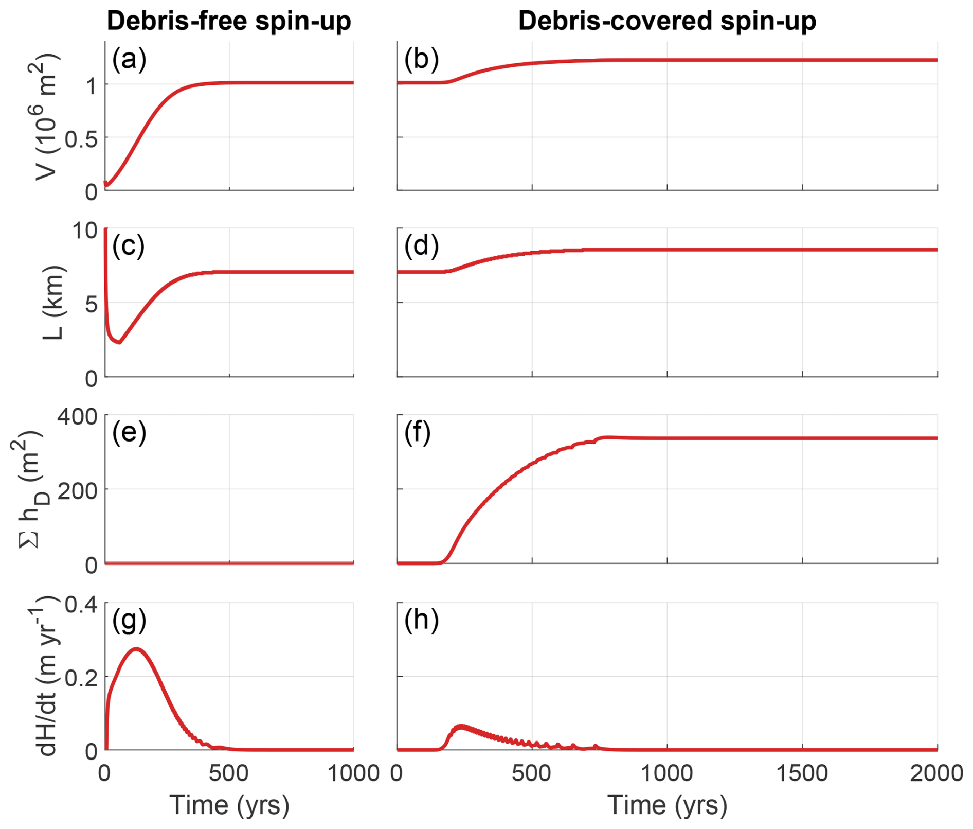
Figure B1 Full model spin-up procedure: (a, b) ice volume, (c, d) glacier length, (e, f) total supraglacial debris volume, and (g, h) glacier-averaged change in ice thickness ($\partial H/\partial t$) evolving over two spin-up periods. First, an initial debris-free spin-up period of 1000 years, initialized from 10 m of ice thickness along the entire bed at time 0. Second, a steady debris input is introduced and the simulation is run for 2000 years, when the modelled glacier has reached a steady-state for any steady-state parameter set.

B2 Repeat-experiments: debris input rate and position in steady-state

Here, we repeat modelling experiments similarly conducted by Anderson and Anderson (2016) and Ferguson and Vieli (2021). The results found here are qualitatively very similar to their findings, supporting the validity of our approach.

In this experiment, we force the model with different, but time-constant debris input rates (Fig. B2). We explore a range of debris input rates from the lowest estimate from Anderson and Anderson (2016), 1 mm yr⁻¹, up to 5 times of their average rate, an extreme of 22.5 mm yr⁻¹. Between input rates, the glacier surface profiles are still very similar to each other, but substantially more elongated with increasing debris input rate d_in (Anderson and Anderson, 2016). Total surface debris volume (Fig. B2c) thereby scales non-linearly with increasing d_in, as both local debris cover thickness and the covered glacier length increase. The mass balance gradient (Fig. B2b) starts to be reversed in the upper debris-covered area with increasing debris input, but stabilizes relatively quickly further below as the increasing, elevation-dependent clean-ice ablation (e.g., −6 m yr⁻¹ at 2100 m a.s.l.) is compensated but not surpassed by insulation from debris thickening.

In a next step, we assess the impact of the debris deposition location by comparing two accumulation area cases (Fig. B3), one closer to the headwall than the other, and one ablation area case, set up similarly by Anderson and Anderson (2016). We observe that when moving debris input closer to the ELA, the englacial transport trajectory gets shorter and the debris melt-out area moves up-glacier, with the glacier ultimately increasing in length. The ablation area case, with the debris input closest to the ELA, leads to the largest debris-covered area (Fig. B3c) and consequently to the most elongated glacier, as ablation is reduced already further up-glacier and therefore over a larger part of the ablation area (Fig. B3b), which is in line with the earlier modelling by Anderson and Anderson (2016). In general, the impact on steady-state glacier length from changing debris input locations remains in our case relatively small (below a few percent) and the maximum debris thickness at the terminus is rather similar for all cases with our reference parameter set. As Anderson and Anderson (2016) describe, the impact of debris input location increases with increasing input rate.

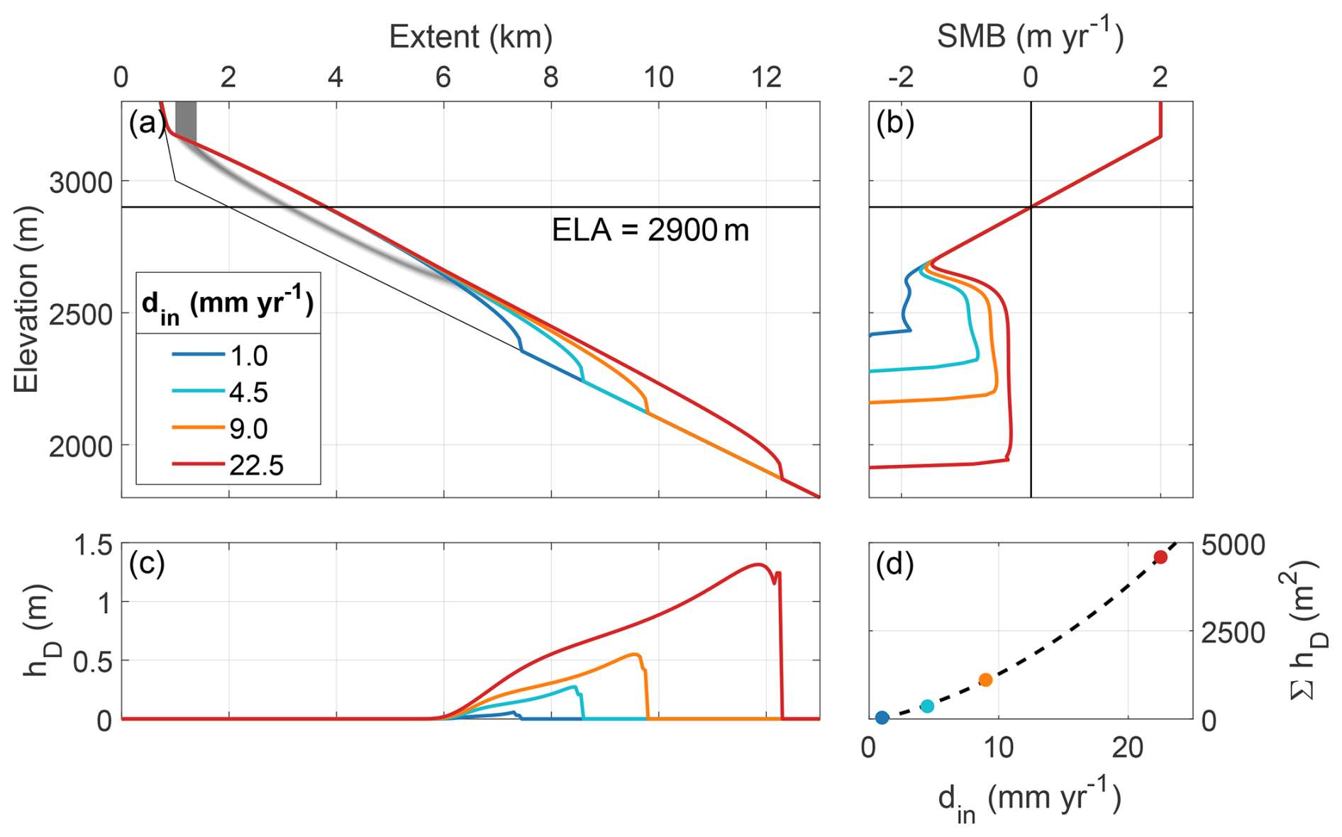
Figure B2 Steady-state glaciers for variable debris input rates d_in (1.0, 4.5, 9.0, and 22.5 mm yr⁻¹) with otherwise the same parameter setting as in Fig. 2 with the resulting steady-state (a) glacier surface geometries, (b) surface mass balance, and (c) debris cover thickness h_D. The gray area marks the debris input area below the headwall and the englacial debris transport trajectory.

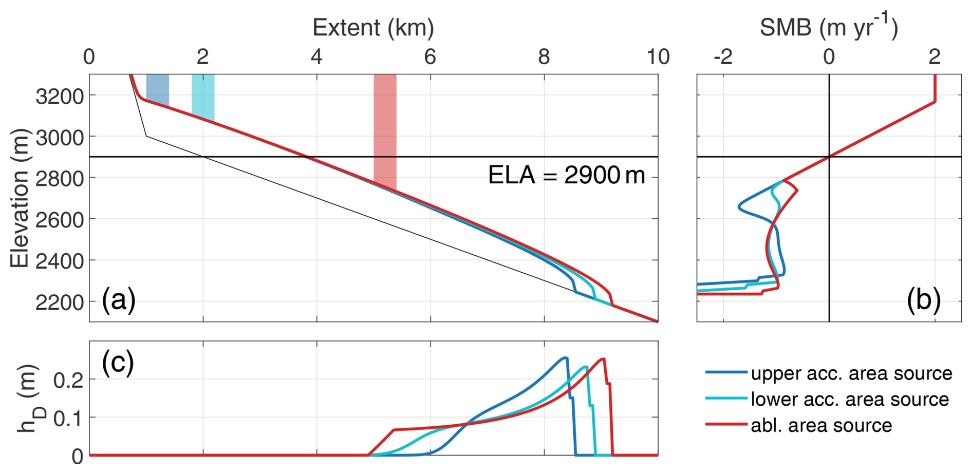
Figure B3 Steady-state glaciers for different debris input area locations (0, 800, and 4000 m from headwall slope break) using the same debris input rate of 4.5 mm a⁻¹ and an ELA of 2900 m with the resulting steady-state glacier (a) surface geometries, (b) surface mass balance, and (c) debris cover thickness h_D.

B3 Additional time transient modelling experiments

Below, two additional experiments of time transient forcings in debris and climate input are presented. Figure B4 shows the effect of a long-term (century-scale) fluctuation in debris input position. Similarly to the steady-state case (Fig. B3), we observe a relationship between along-flow position of debris input and the extent of the down-glacier debris covered area. Unique to the transient case is a large variation near the terminus, connected to dynamic stagnation (Fig. B4b) whenever debris cover decline leads to lower mass balance.

Figure B5 compares debris-free and debris-covered glaciers in their transient response to oscillations in ELA. By comparing glaciers with equivalent (steady-state) volume, we can account for other dynamic effects on the response and show that debris-covered glaciers are less reactive than debris-free glaciers of comparable size, both in volume (Fig. B5b) and length (Fig. B5c).

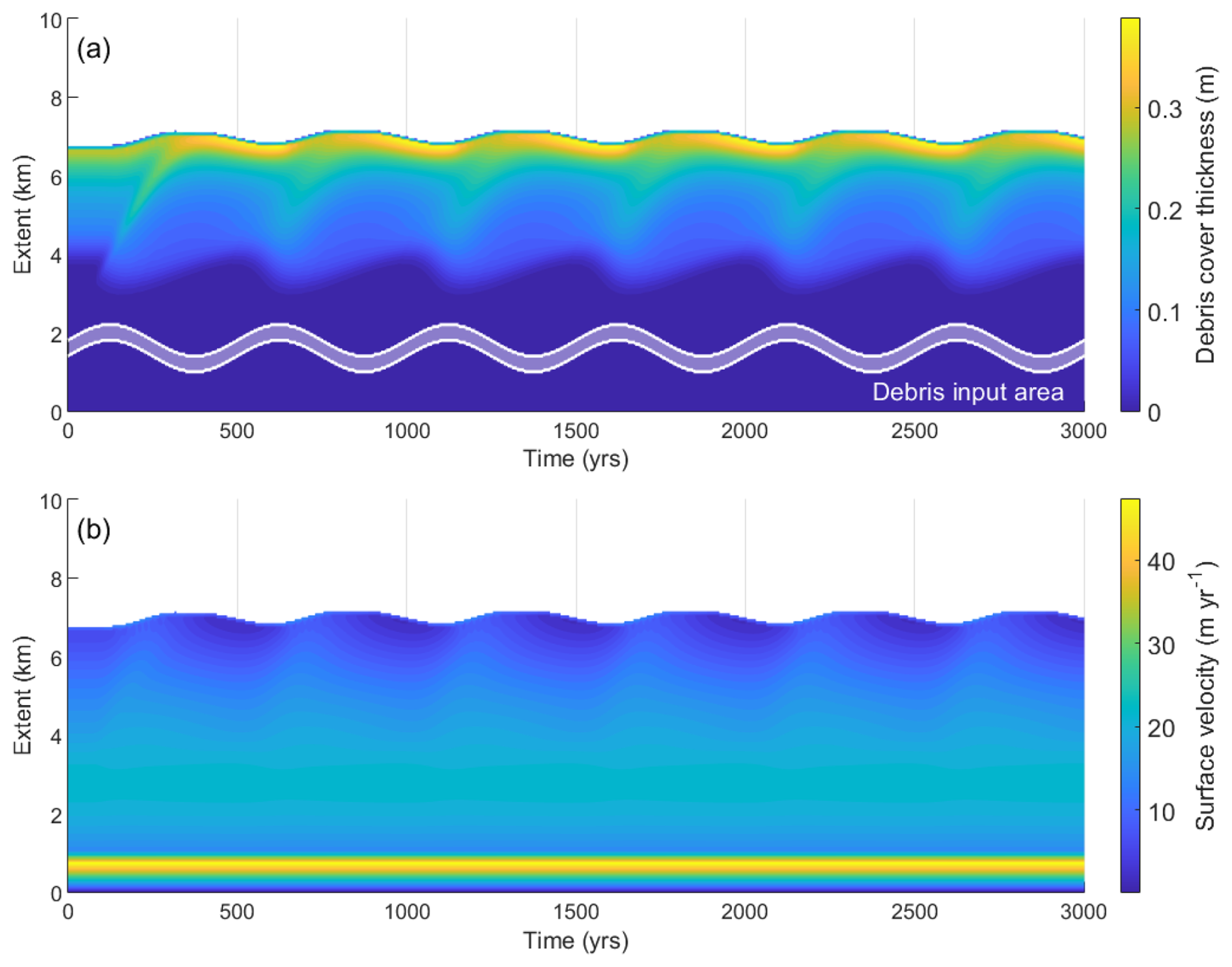
Figure B4 Varying debris input position in a sine wave (wavelength = 500 years, amplitude = 800 m with $\mathrm{1000}\mathrm{m}\le x_{\mathrm{d}}\le \mathrm{1800}$ m, ELA = 3000 m). (a) Debris cover thickness response and (b) surface velocity over time and along-glacier extent.

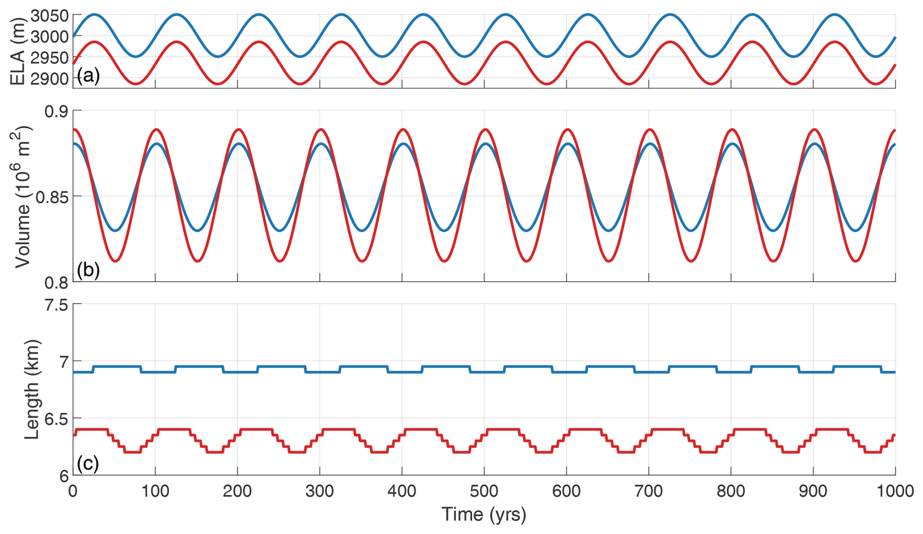
Figure B5 Sine wave climate experiment comparing a a clean-ice (red) to a debris-covered (blue) glacier. (a) ELA oscillating with an amplitude of 50 m and λ=100 years around 2935 (clean-ice) and 3000 m a.s.l. (debris-covered). This corresponds to equal steady-state volumes, enabling a direct comparison of dynamic response: (b) glacier volume and (c) length response.

Appendix C: Model robustness and parameter sensitivity

In this section, we conduct experiments to test the robustness of the model performance in transient behavior, using strongly idealized setup and parameters. This includes the examination of model sensitivity to parameter variability on an individual basis. We further explore and discuss aspects of the model in terms of long-term reversibility when returning to the initial forcing state (Appendix C1), grid size dependence, and debris mass conservation (Appendix C2).

C1 Model reversibility

As noted in Sect. 3.3.1 and 3.3.2, steady-state terminus positions can slightly differ for identical parameter sets based on previous states. Experiments clim-1 and deb-1 (Figs. 4, C1 and C2) show that reaching a steady-state from a previously more debris-covered state (higher ELA or d_in) leads to a slightly more advanced terminus position than in the previous less debris-covered state. The discrepancy is more enhanced (400 m) in experiment deb-1, where we directly affect debris cover by altering the debris input quantity, in comparison to the ELA change experiment clim-1 (50 m), where the impact on debris cover is indirect through a change in accumulation rate, while keeping the total debris input rate the same (Fig. C3). In the latter case, a glacier carries more total debris on its surface when in a warmer state (Fig. 4e and f).

We further explore the range of possible states (Fig. C1) for a single set of parameters, which shows the resulting length for a wide variety of temporary d_in step-change magnitudes (a) and durations (b). For both amount and duration we see a slight increase in post-event steady-state length, confined by a maximum length, which seems to represent the longest glacier that can be sustained with this particular steady-state set of forcing variables. Conversely, coming from a less debris-covered initial state will always result in the minimum stable state (red line in Fig. C1a and c), and hence is reversible, even if preceded by a more debris-covered state.

To further investigate whether this discrepancy is purely a numerical issue arising from the implementation of the terminal boundary condition (as described in Sect. 2.4), we conduct an additional experiment. The ice cliff thickness parameter H^*, otherwise considered a model parameter fixed at 30 m, is in this experiment oscillating as a sine wave between 10 and 50 m at a decadal time-scale (λ=40 years), emulating a cyclically forming and collapsing terminal ice cliff. In this configuration, debris is removed more efficiently at the terminus, leading to a generally less elongated steady-state glacier after retreat. Our results (Fig. C4) suggest that, even with large variations in cliff height, the difference to the initial state, though more subdued, persists. Still, the debris cover profiles (Fig. C4b) are only distinguishable between the initial and elongated states in the immediate vicinity of the terminus, leading us to the conclusion that the discrepancy is most likely connected to the terminal boundary implementation and not an observable dynamic feedback.

Overall, our results emphasize that the modelled steady state glacier length is in our modelling strictly speaking not reversible and dependent on the previous state of debris cover, but in our experiments the effect stays small (a few percent) and importantly it only affects the debris thickness and glacier geometry in the terminal few 100 m. Furthermore, in nature climate is rapidly fluctuating and this steady-state effect not really observable. For consistency in our modelling experiments we always start our experiments with the minimum steady-state as initial condition.

C2 Debris mass conservation

Mass conservation is a well-known issue for advection schemes such as ours, where parts of the advected quantity can diffuse. This reflects itself in inconsistent debris fluxes, where input does not always equal output. Previous approaches have either made no mention of the issue (e.g., Anderson and Anderson, 2016) or applied a correction factor to account for missing debris (e.g., Mayer and Licciulli, 2021). Here, we aim to give a detailed account of the discrepancies we encountered in our approach and how we avoid them having a large effect on our results. In Fig. C5 we examine the along-glacier debris flux Q_d, spatially resolved, for a set of steady-states with ELAs ranging from 2700 to 3200 m. We find that, as long as the debris input zone is well above or well below the ELA (here: debris input occurs roughly between 3100 and 3175 m, hence for ELAs below 3000 m or from 3200 m upwards), the total debris flux, consisting of the sum of englacial and supraglacial flux, is almost entirely conserved (debris output >97 % of input). However, as soon as the ELA is at a similar elevation as the debris input zone (e.g., 3100 m), the debris flux is substantially reduced (by about 35 %), which means debris is lost. This issue is restricted to the specific case where debris is deposited onto the glacier in close proximity of the ELA, which we consciously avoid in our experiments.

C3 Convergence regarding grid spacing

To show numerical convergence and the upper boundary of suitable grid spacing values, we perform additional tests. Figure C6 shows steady-state glacier simulations at resolutions ranging from 25 to 200 m. While glacier states converge reasonably well at grid spacing up to 100 m, model performance drastically reduces at coarser spacing. There, the narrow debris input area is reduced to a few grid cells, and the terminus appears in a substantially receded position. We infer that our approach performs well at grid spacing of 100 m or lower, where results become virtually indistinguishable.

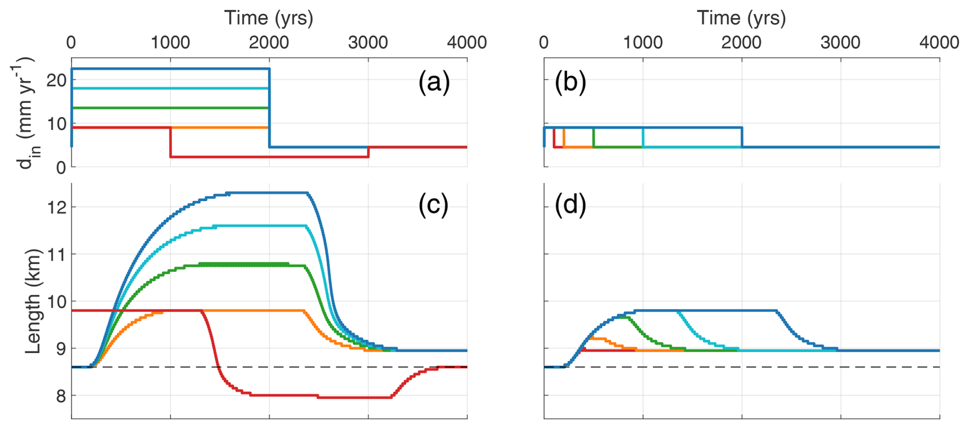
Figure C1 Debris input step-change experiments deb-1: (a) increasing d_in at time zero from 4.5 mm yr⁻¹ to double (orange), triple (green), quadruple (cyan), quintuple (blue), as well as doubling followed by halving (red) after 1000 years. After 2000 years the debris input is reset to the initial value. (b) Varying duration of debris input doubling d_in experiment: 100 (red), 200 (orange), 500 (green) 1000 (cyan), and 2000 years (blue). (c, d) Corresponding glacier length responses.

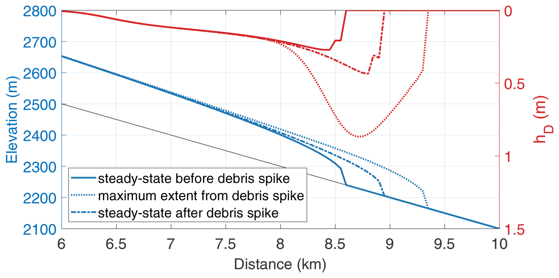
Figure C2 Geometry adjustment in short-term debris input spike experiment (Exp. deb-2; Fig. 6): glacier geometry (blue) and debris cover thickness (red) at three relevant points in time: at the steady-state before the first spike event (solid lines), at maximum extent caused by the spike (dotted lines), and at the new steady-state after the event (dashed lines).

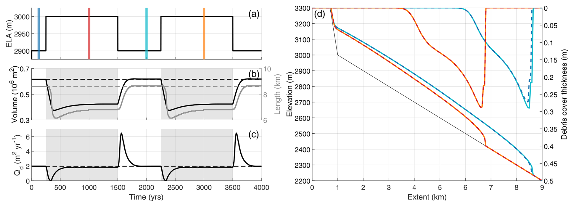
Figure C3 Repeated 100 m ELA step-change experiment: (a) ELA forcing and markings for the four steady-states shown in (d). (b) Glacier volume and length response, (c) near-terminus debris flux response. (d) Four steady-state glacier geometries as marked with the colored bars in (a), at 2900 m (blue, cyan) and 3000 m (red, orange) ELA.

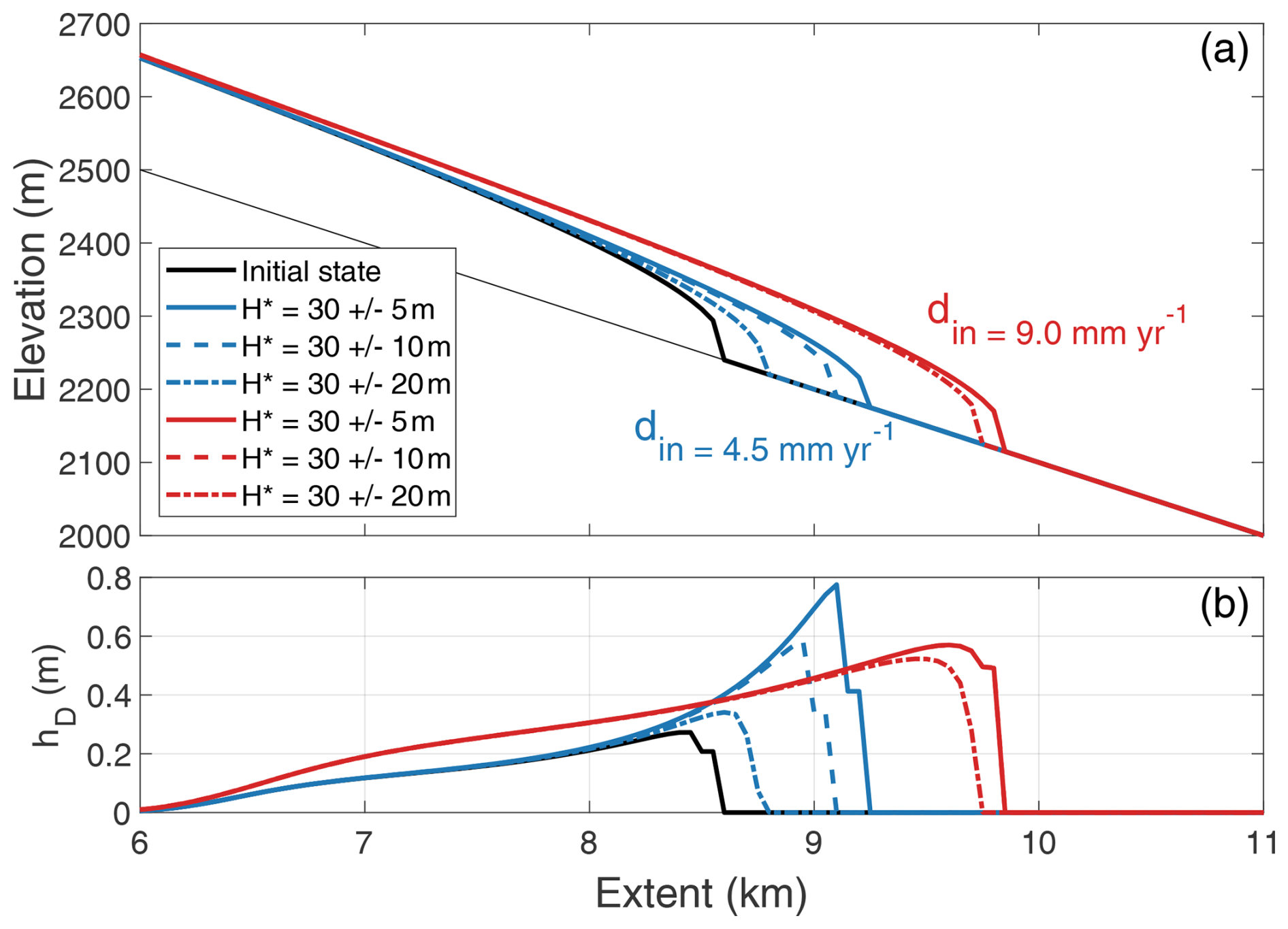
Figure C4 Influence of variable terminal cliff height H^* on terminus position relative to the initial (undisturbed) position: (a) geometry of the debris-covered ablation area for the following cases: initial steady-state (black), advanced, d_in-enhanced steady-state (red), and post-advance state with the initial standard parameter set (blue). The disturbances are implemented as sine waves in H^* (λ=40 years) with amplitudes of 5 (solid line), 10 (dashed), and 20 (dash-dotted) m, respectively. (b) Along-flow debris thickness profile of the cases described in (a).

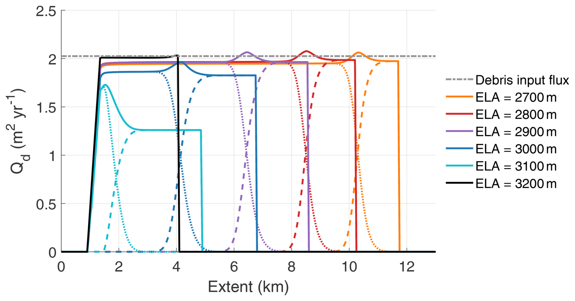
Figure C5 Along-glacier debris flux Q_d for 6 different ELA steady-states (2700–3200 m a.s.l.) given a constant d_in of 4.5 mm yr⁻¹. The total debris flux Q_d (solid lines) consists of the sum of the englacial (dotted lines) and the supraglacial (dashed lines) fluxes. The gray dash-dotted line represents the debris input flux $Q_{\mathrm{d},\mathrm{in}}=d_{\mathrm{in}}{L}_{\mathrm{d}}$.

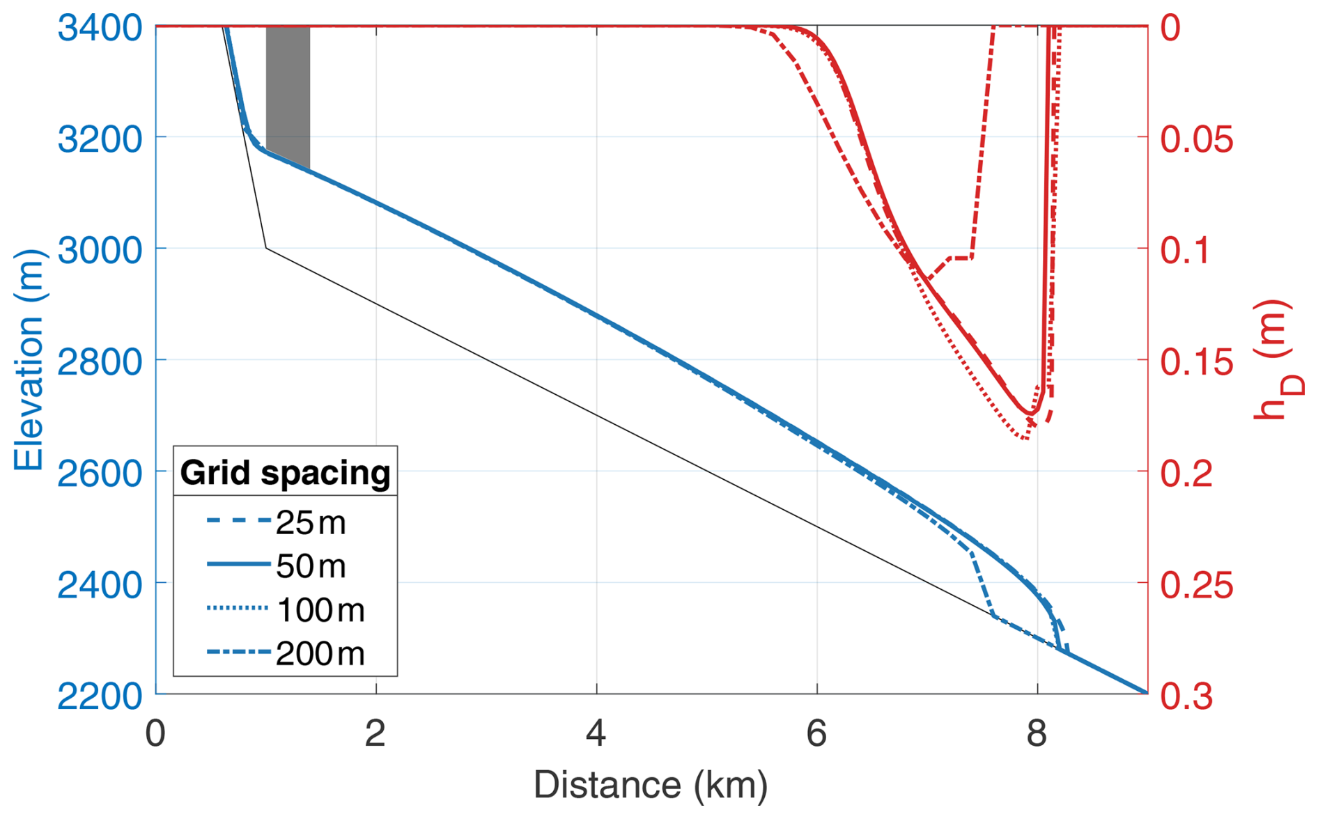
Figure C6 Glacier geometry (blue) and debris thickness (red) for steady-state glaciers at a grid spacing of 25, 50, 100, and 200 m, respectively. The gray shaded area indicates the debris input area.

Appendix D: Sensitivity to standard model parameters

For Glen's flow law rate factor A and the characteristic debris thickness D₀, both assumed as constant model parameters in our experiments, we found a range of values in literature. These parameters also depend on conditions like ice temperatures or lithology and should be constrained by empirical evidence when modelling a specific glacier. Here we examine the impact in transient response from a sensible range of model parameters based on the literature (Anderson and Anderson, 2016; Ferguson and Vieli, 2021) and empirical data (Fontrodona-Bach et al., 2025). The sensitivity of the transient model response to these variables was tested in a standard ELA step-change experiment (clim-1), where sudden warming is followed by sudden cooling.

D1 Sensitivity to rate factor A

The rate factor A is a constant in Glen's flow law (Eq. A2) describing ice creep and dominantly depends on ice temperatures. Following the power law function with temperature (Cuffey and Paterson, 2010), temperate glaciers (T=0 °C), should have a value of A of $\mathrm{2.4}\times {\mathrm{10}}^{-\mathrm{24}}$ s⁻¹ Pa⁻³. For lower temperatures, A decreases significantly (e.g., $\mathrm{0.93}\times {\mathrm{10}}^{-\mathrm{24}}$ s⁻¹ Pa⁻³ for −5 °C). Data on ice temperatures in debris-covered glaciers is scarce. A recent study from Khumbu glacier shows polythermal conditions (Miles et al., 2018), with temperatures ranging from 0 to −3 °C. In temperate climates with substantial surface melt in the accumulation area, such as the Alps, temperate ice conditions are prevailing (Suter et al., 2001). The rate factor can also be enhanced due to impurities within the ice (Cuffey and Paterson, 2010), but this effect is secondary and less well-constrained.

Similar as for clean-ice glaciers, for the initial steady state (ELA of 2900 m), we find a clear impact from a variable A on the glacier geometry (length and volume). A higher A leads to more ice deformation, which causes faster ice flow for the same thickness and ultimately results in a thinner and hence shorter glacier (Fig. D1). After a step-increase in ELA, we find that the transient response (relative length and volume change) is only weakly sensitive to the rate factor. Response times decrease only slightly for a high ($\mathrm{2.4}\times {\mathrm{10}}^{-\mathrm{24}}$ s⁻¹ Pa⁻³) value of A, because the enhanced velocities from an increase in A accelerates geometric adjustment. We conclude that the transient response remains qualitatively similar irrespective of the choice in the rate factor, while quantitatively glacier geometry itself (and thus volume) is sensitive to A.

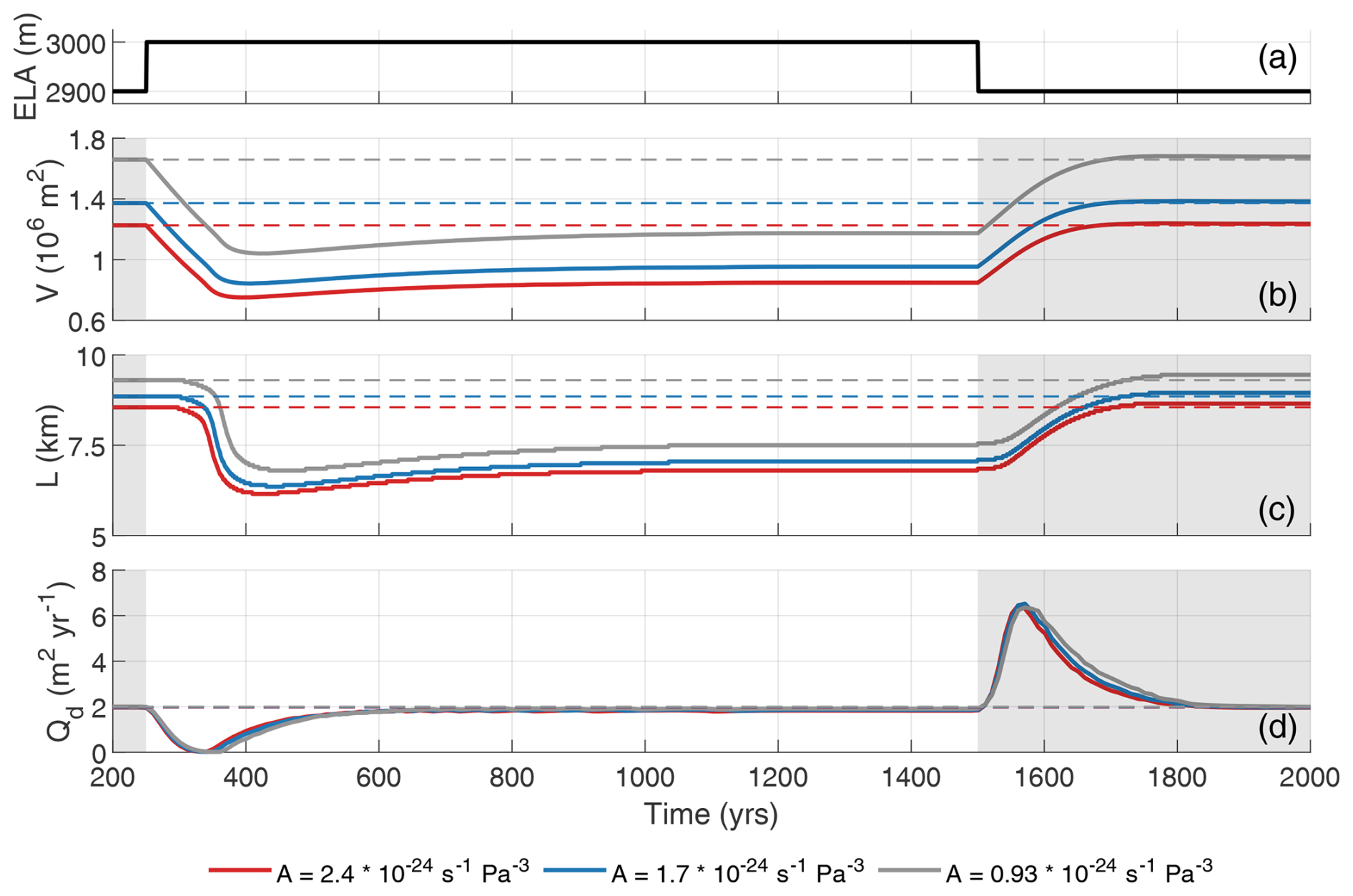
Figure D1 Transient sensitivity of the model for variable rate factors A when applying a step-change ELA forcing (a). (b) Volume response, (c) length response, and (d) debris flux Q_d response 100 m up-glacier from the terminus.

D2 Constraining of and sensitivity to the characteristic debris thickness D₀

The characteristic debris thickness D₀ describes how much insulation a given debris thickness can provide, or in other words, how fast the Østrem curve descends (the lower D₀, the more insulation, the less melt). Therefore, changing D₀ by several cm leads to substantially different initial steady-state geometries (see initial length and volume in Fig. D2). Estimates of D₀ can vary substantially between glaciers and studies (Fontrodona-Bach et al., 2025). Here, we examine the sensitivity of model results to values ranging between 0.05 and 0.15 m. Qualitatively, the transient response is somewhat affected by changes in D₀ (Fig. D2). Following the warming period, a low D₀ value (stronger insulation) results in a prolonged stagnant thinning phase (later retreat), a more abrupt but delayed retreat phase, and a longer, more pronounced rebounding effect. This emphasizes the need for an accurate estimate of D₀ for modelling the evolution of a particular glacier. For the advance case, after a step-lowering of the ELA, the increase in ice flux and velocities combined with the already elongated tongue from a lower D₀, gives rise to a more pronounced temporary debris flux surplus (Fig. D2d). However, this has no substantial consequence on the advance response (Fig. D2b and c). In general, the choice of D₀ does not affect the main conclusions made in this study.

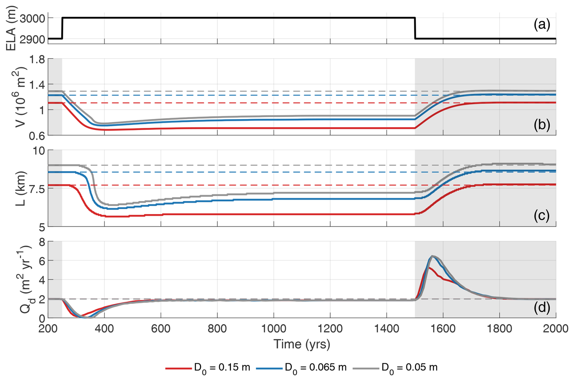
Figure D2 Transient sensitivity of the model for variable characteristic debris thickness D₀ when applying a step-change ELA forcing (a). (b) Volume response, (c) length response, and (d) debris flux Q_d response 100 m up-glacier from the terminus.