Enabling ice sheet models to capture centennial-scale solid Earth feedback with relative ease and sufficient accuracy

There is a growing consensus on the critical role that solid Earth processes play in influencing marine ice sheet dynamics over centennial timescales. A large body of literature shows that the feedback mechanisms associated with the solid Earth's gravitational, rotational, and deformational (GRD) response to ice mass loss slow the progression of ice sheet instabilities. However, due to the limited availability of efficient coupled system models, the specific characteristics of the feedback mechanisms, their sensitivities to ice sheet processes, and their impacts on centennial-scale sea level projections remain largely unexplored. This paper introduces a simple method that enables ice sheet models to address this limitation by capturing GRD effects with relative ease and sufficient accuracy. The proposed method uses precomputed Green's functions for a suite of radially symmetric Earth models and convolves them with mass changes within the ice sheet model. This approach straightforwardly retrieves the induced geoid and bedrock topography fields, paving the way for efficient coupling between ice sheet dynamics and leading-order solid Earth response on decadal to centennial timescales.

1 Introduction

An improved understanding of ice sheet dynamics is essential for producing accurate global and regional sea level projections. To achieve this, sophisticated ice sheet models that capture higher-order processes and feedback mechanisms are necessary. The ice sheet modeling community has increasingly recognized the importance of dynamic interactions between ice sheets and solid Earth processes over decadal and longer timescales. As ice mass changes, it exerts spatiotemporal variations in pressure on the solid Earth surface, changing bedrock topography and the geoid field, and thus sea level. These alterations in topography and sea level significantly influence marine ice sheet dynamics. They do so by affecting the retrograde bed slope, reinforcing pinning points and bedrock ridges, altering ocean heat transport patterns due to the modified shape of sub-shelf cavities, and influencing gravitational driving stress and surface mass balance through surface elevation and slope changes (e.g., Gomez et al., 2012; Adhikari et al., 2014; Larour et al., 2019; Albrecht et al., 2024; Kreuzer et al., 2025).

Several established methods of varying complexity exist for capturing solid Earth feedback in ice sheet models. The most straightforward approach relies on the two-layer framework of Lingle and Clark (1985), consisting of an elastic lithosphere overlying a viscously relaxing mantle half-space (e.g., Ivins and James, 1999; Adhikari et al., 2014; Swierczek-Jereczek et al., 2024). Building on this, Meur and Huybrechts (1996) introduced a formulation in which the lithosphere overlies a finite-thickness asthenosphere layer, commonly referred to as the Elastic Lithosphere Relaxing Asthenosphere (ELRA) model. A more complex method involves modeling a self-gravitating, density-stratified, viscoelastic Earth with a radially symmetric structure that typically includes an elastic lithosphere, a multi-layered Maxwellian mantle, and an inviscid core (e.g., Peltier, 1974; Farrell and Clark, 1976). Generally used in glacial isostatic adjustment (GIA) studies, this class of models enables capturing the full gravitational, rotational, and deformational (GRD) feedback to ice sheet dynamics (e.g., Gomez et al., 2012; Konrad et al., 2015; Larour et al., 2019; Han et al., 2022). More comprehensive approaches, such as those involving three-dimensional Earth structure (e.g., Albrecht et al., 2024; Gomez et al., 2024) and sophisticated non-Maxwellian mantle rheology (Houriez et al., 2025; Coonin et al., 2026), are currently being explored to enhance our understanding of feedback mechanisms.

All these models come with caveats, especially regarding their suitability for high-resolution coupled simulations. Downsides may range from being too simplistic (e.g., half-space models) to involving complex numerical implementations that demand significant computational cost (e.g., global GIA models). As a result, many ice sheet models, including those involved in the Ice Sheet Model Intercomparison Project (ISMIP), often omit GRD feedback. Among the 16 models that contributed to the ISMIP Antarctic Ice Sheet projections extending to 2300 (Seroussi et al., 2024), only four include any representation of solid Earth feedback, and even these primarily rely on the most simplified ELRA approach. The omission of GRD feedback, or its representation through the ELRA approximation, may bias projections of grounding line retreat and sea level change (e.g., Konrad et al., 2016; Larour et al., 2019). GIA emulators (Lin et al., 2023; Love et al., 2024) and more realistic regional models (Coulon et al., 2021; Swierczek-Jereczek et al., 2024; van Calcar et al., 2026) are emerging as promising options that offer reduced computational cost. Further investigation is needed into both traditional geophysical modeling approaches and emerging machine learning techniques to improve model efficiency and accuracy and simplify the coupling strategy.

Here we present a simple method that enables ice sheet models to capture solid Earth feedback requiring neither additional model development nor computational cost. A primary motivation for this research is to enhance ISMIP’s current and future undertakings by enabling greater participation in coupled ice/Earth simulations, with direct implications for future Intergovernmental Panel on Climate Change (IPCC) reports that cater to planners and policymakers. We therefore focus on capturing the leading-order feedback signals over centennial timescales for radially symmetric Earth structures. We show that the direct effects of ice mass change account for over 90 % of the self-consistent GRD feedback signals in a radially symmetric Earth. In order to capture this leading process, it suffices to convolve the evolving mass change with time-variable Green’s functions that characterize the solid Earth response to unit surface loads. By leveraging an extensive library of precomputed Green’s functions available for a suite of Maxwellian Earth structures (Adhikari and Caron, 2024), our proposed method facilitates the swift retrieval of the evolving geoid and bedrock topography fields as ice sheet models march forward in time, thus enabling straightforward coupling between the ice sheet and the solid Earth. An efficient coupling enhances our understanding of feedback mechanisms, facilitates sensitivity analysis, and strengthens uncertainty quantification through large ensemble simulation. Ultimately, these improvements will enable more reliable projections of ice sheet contribution to sea level change.

The proposed method differs fundamentally from the commonly used ELRA framework. Rather than approximating Earth response through lithospheric flexural rigidity and asthenospheric relaxation timescales, the Green's functions employed here are derived from solutions of the governing equations of mass conservation, linear momentum conservation, and self-gravitation for a full-depth multilayered viscoelastic Earth (Caron et al., 2026). This provides a more realistic representation of load-induced deformation and gravitational signals, consistent with the framework adopted in modern GIA modeling. Moreover, standard ELRA implementations typically neglect geoid change and associated gravitational feedbacks, focusing solely on bedrock adjustment. As will be demonstrated below, geoid variations can be significant and are largely governed by ice mass changes. Accounting for these effects is therefore essential in coupled ice/Earth simulations.

Like any simplified/regional method, ours comes with limitations. It does not satisfy self-consistency in GRD processes (Farrell and Clark, 1976; Milne and Mitrovica, 1998), nor does it conserve mass in the global domain of ice and ocean. The effects of rotational feedback (Milne and Mitrovica, 1998), farfield ice melting (Gomez et al., 2020), and coastline migration (Kendall et al., 2005) are ignored. Although we show that these processes play a secondary role on the timescale of interest, they are critical in longer-timescale simulations (e.g., glacial cycles) and they can only be accounted for by recursively solving the self-consistent sea level equation (e.g., Spada and Melini, 2019). Our method does not capture the effects of three-dimensional Earth structures (Gomez et al., 2020), although the appropriate choice of a regionally averaged one-dimensional structure may partially mitigate this deficiency (Albrecht et al., 2024; Han et al., 2025; van Calcar et al., 2026). We caution readers of these caveats for the appropriate use of our method, whose main purpose is to capture solid Earth feedback in centennial-scale simulations of modern or paleo ice sheets.

2 Proposed method

Assuming that atmospheric pressure variability does not induce meaningful solid Earth deformation on decadal and longer timescales, the surface loading problem in the present context only requires resolving the lateral mass transport between the ice sheet and the ocean. A conditional function describing the ice and ocean load on the solid Earth surface, termed the “loading function” L [kg m⁻²], at a given point in time t may be expressed as follows:

$$\begin{array}{}\text{(1)}& L(\mathit{x},t)=\begin{array}{l}{\mathit{\rho }}_{\mathrm{i}}H(\mathit{x},t)\text{if}H(\mathit{x},t)>F(\mathit{x},t)\\ {\mathit{\rho }}_{w}R(\mathit{x},t)\text{otherwise.}\end{array}\end{array}$$

Here x is the 2-D position vector on the solid Earth surface, ρ_i is the ice density [kg m⁻³], ρ_w is the ocean density [kg m⁻³], H is the ice thickness [m], R is the relative sea level [m], and F is the flotation height for ice [m] (see Fig. 1).

Following Gregory et al. (2019), we define R as the mean sea level S [m] relative to the sea floor, both referenced to the same ellipsoid (typically WGS84). We assume the sea floor is same as the bedrock B [m]. Mathematically,

$$\begin{array}{}\text{(2)}& R(\mathit{x},t)=S(\mathit{x},t)-B(\mathit{x},t).\end{array}$$

In mean sea level S, “mean” refers to a time-mean over tides and high-frequency waves. This distinction is irrelevant in GRD modeling. However, we maintain the terminology to align with the literature.

The flotation height for ice F [m] follows the principle of hydrostatic equilibrium and is given by

$$\begin{array}{}\text{(3)}& F(\mathit{x},t)={\displaystyle \frac{{\mathit{\rho }}_w}{{\mathit{\rho }}_{\mathrm{i}}}}max\left[R(\mathit{x},t),\mathrm{0}\right].\end{array}$$

The condition in Eq. (1) implies that the solid Earth is loaded by the ice sheet in the grounded portion of the marine (and terrestrial) ice sheet and by the ocean otherwise (Fig. 1a).

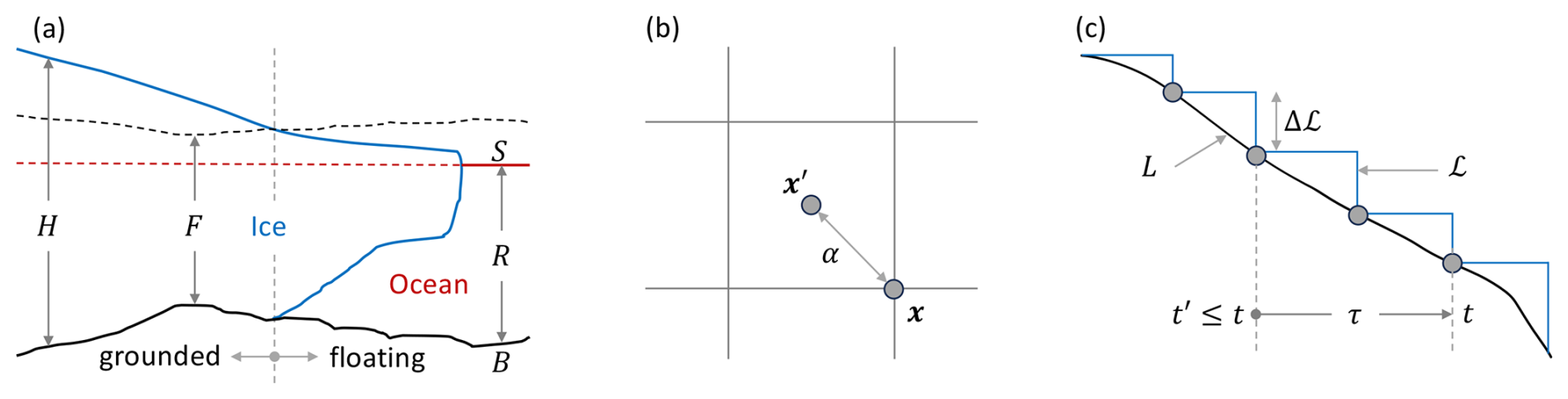
Figure 1 Schematics of the loading function and spatiotemporal grids. (a) Longitudinal cross-section of a marine ice sheet as it flows into the ocean. If ice thickness H is larger than the flotation height F, a function of the bedrock topography B and mean sea level S (Eq. 3), it is assumed to be grounded, exerting pressure on the solid Earth's surface. Elsewhere in the ocean (including the floating ice shelves), ocean water (expressed here as the relative sea level $R\equiv S-B$) loads the underlying solid Earth (Eq. 1). (b) An example spatial grid illustrating the cell centroid x^′, where the elemental surface load is applied (Eq. 4), and the vertex x, where the desired solid-Earth response signal is evaluated (Eq. 5). The two locations are separated by the great circle distance α. (c) Temporal decomposition of the continuous surface load L (diminishing over time in this case) into discrete loading ℒ using the Heaviside step function (Eq. 4). The discrete loading time t^′ and the evaluation time t are separated by τ (see Eqs. 5 and 6).

Numerical modeling requires discretizing the continuous loading function into p computational grids (having q nodes) and m time intervals: $[t_{\mathrm{0}},t_{\mathrm{1}}],[t_{\mathrm{1}},t_{\mathrm{2}}],\mathrm{\dots },[t_{m-\mathrm{1}},t_{\mathrm{m}}]$. Spatial grids and time intervals do not have to be uniformly discretized. We may now express Eq. (1), in the units of mass [kg] and with the new notation ℒ, in its discrete form as follows:

$$\begin{array}{}\text{(4)}& \begin{array}{ll}\mathcal{L}({\mathit{x}}^{\mathbf{\prime }},t)& =\left[\stackrel{\mathrm{‾}}{L}({\mathit{x}}^{\mathbf{\prime }},t_{\mathrm{0}})+\sum _{i=\mathrm{1}}^m\left\{\stackrel{\mathrm{‾}}{L}({\mathit{x}}^{\mathbf{\prime }},t_{\mathrm{i}})-\stackrel{\mathrm{‾}}{L}({\mathit{x}}^{\mathbf{\prime }},t_{i-\mathrm{1}})\right\}\right.\\ & \left.\mathcal{H}(t-t_{\mathrm{i}})\right]A\left({\mathit{x}}^{\mathbf{\prime }}\right),\\ & =\mathcal{L}({\mathit{x}}^{\mathbf{\prime }},t_{\mathrm{0}})+\sum _{i=\mathrm{1}}^m\mathrm{\Delta }\mathcal{L}({\mathit{x}}^{\mathbf{\prime }},t_{\mathrm{i}})\mathcal{H}(t-t_{\mathrm{i}}),\end{array}\end{array}$$

Here x^′ is the position of the center of the grid-cell or element, A is the elemental area [m²], and $\stackrel{\mathrm{‾}}{L}$ [kg m⁻²] is the spatial mean of L over that area. As shown in Fig. 1b, we recommend placing the surface load at the grid centers, x^′, instead of at the nodes or vertices, x, where we assess the solid Earth response. This is important because the Green's functions we intend to use contain inherent singularities at the loading point (Longman, 1962). In the equation, ℋ is the Heaviside step function that takes the value of unity for t≥t_i and zero otherwise. It ensures that we impose the stepwise load change on the solid Earth surface at the end of each time interval (Fig. 1c). For the period $-\mathrm{\infty }<t<t_{\mathrm{1}}$, the surface load is held constant to its initial or reference value $\mathcal{L}({\mathit{x}}^{\prime },t_{\mathrm{0}})$, and we assume that the solid Earth is in hydrostatic equilibrium. As such, only the change in load induces solid Earth response, which can be evaluated at any time t≥t₁.

For m=1 and in the limit of p→∞ for a structured mesh (or, equivalently, A→0) , setting in Eq. (4) the otherwise zero loading function to unity strictly at a single computational grid and at time t=t_m corresponds to a mathematical description of a point load. Harmonic solid Earth response to a point load sustained on the surface of a radially symmetric layered solid Earth is traditionally computed as the time-dependent Love numbers (Love, 1909; Shida, 1912). We may assemble the Love numbers analytically to determine Green's functions (Appendix A). Given these functions, we can retrieve the solid Earth response signals induced by the loading function with any complexity through direct spatiotemporal convolution:

$$\begin{array}{}\text{(5)}& X(\mathit{x},t)=K_X(\mathit{\alpha },\mathit{\tau })\otimes \mathrm{\Delta }\mathcal{L}({\mathit{x}}^{\prime },t^{\prime }),\end{array}$$

where X is the GRD field of interest [m], K_X is the corresponding Green's function [m kg⁻¹], α is the (great circle) distance between the loading position x^′ and where the response signal is determined x, and τ is the time elapsed between the loading time t^′ and when the response signal is evaluated t (Fig. 1). Let ϕ and λ be the geographic latitude and longitude of the evaluation and loading points: $\mathit{x}\equiv (\mathit{\varphi },\mathit{\lambda })$ and ${\mathit{x}}^{\prime }\equiv ({\mathit{\varphi }}^{\prime },{\mathit{\lambda }}^{\prime })$, respectively. Then, the distance between the two points can be written as $\mathit{\alpha }=r\left[\mathrm{2}\arcsin \sqrt{{\sin }^{\mathrm{2}}\left(\frac{|\mathit{\varphi }-{\mathit{\varphi }}^{\prime }|}{\mathrm{2}}\right)+\cos \mathit{\varphi }\cos {\mathit{\varphi }}^{\prime }{\sin }^{\mathrm{2}}\left(\frac{|\mathit{\lambda }-{\mathit{\lambda }}^{\prime }|}{\mathrm{2}}\right)}\right]$, where r is the Earth's surface radius. Note that Δℒ in the equation represents the change in load over the preceding interval to the loading time (Fig. 1c).

In the present context, X denotes either the geoid change G [m] or vertical land motion (VLM). In GIA/GRD theory, where sea level change is due to lateral mass exchange between and within land (including Cryosphere) and the ocean, these quantities are directly related to relative sea level (Eq. 2). The geoid is an equipotential surface of Earth’s gravity field that coincides with the mean sea level S over the ocean, while VLM represents change in bedrock elevation B (Gregory et al., 2019).

The convolution operator ⊗ appearing in Eq. (5) can be straightforwardly evaluated with scientific computational tools. For example, the desired GRD signal X at a given point in space x_k and time t and can be evaluated as follows:

$$\begin{array}{}\text{(6)}& X({\mathit{x}}_k,t)=\sum _{j=\mathrm{1}}^p\sum _{i=\mathrm{1}}^m{K}_X({\mathit{\alpha }}_{k,j},{\mathit{\tau }}_{\mathrm{i}})\mathrm{\Delta }\mathcal{L}({\mathit{x}}_j^{\prime },t_{\mathrm{i}}^{\prime }),\text{for}{t}_{\mathrm{m}}^{\prime }\le t,\end{array}$$

with p and m being the total number of loading points in space and time, respectively, and ${\mathit{\tau }}_{\mathrm{i}}=t-t_{\mathrm{i}}^{\prime }$. The GRD field can be obtained by iterating over discrete points $k\in [\mathrm{1},q]$, where q is the total number of computational nodes (Fig. 1b). For simulations of ice/Earth coupling at centennial timescales, we expect q to be several orders of magnitude larger than m (a direct function of coupling interval, typically 10 years). A more efficient convolution approach could involve retrieving the GRD field induced by a Heaviside load and iterating along the time dimension. Appendix B presents an algorithm for such a scheme.

3 Solid Earth Models

A key novelty of the proposed method is the use of a precomputed library of Green’s functions that characterize the solid Earth response to applied surface point loads. We calculate time-dependent Love numbers for 644 radially stratified Maxwellian Earth models (Adhikari and Caron, 2024). We also derive corresponding Green's functions, relevant for estimating vertical and horizontal land motion and geoid change. These solutions are based on seismologically constrained density and elastic Earth structure, informed by high-pressure and high-temperature mineral physics (Dziewonski and Anderson, 1981), and incorporate a sufficiently broad range of lithosphere thickness and upper mantle viscosity to investigate solid Earth responses to ice sheet evolution on decadal to centennial timescales, at both individual and multiple drainage basin scales.

Solutions are available for 23×28 combinations of lithosphere thickness and upper mantle viscosity. We linearly sample 23 lithosphere thicknesses between 30 and 250 km at 10 km intervals. Upper mantle viscosity samples include $\mathrm{1}:\mathrm{9}\times {\mathrm{10}}^{\mathrm{18}}$ Pa s (9 samples), $\mathrm{1}:\mathrm{9}\times {\mathrm{10}}^{\mathrm{19}}$ Pa s (9 samples), and $\mathrm{1}:\mathrm{10}\times {\mathrm{10}}^{\mathrm{20}}$ Pa s (10 samples), while the lower mantle viscosity is fixed at 2×10²² Pa s for all models. Time-dependent Love numbers and Green’s functions are sampled in log-space at 100 snapshots between 0 year (purely elastic signal) and 1000 years. Logarithmic sampling better captures early-time deformation following loading or unloading when the response evolves more rapidly (Figs. 2 and A1). Because the main purpose of this study is to enable centennial-scale simulations, we restrict sampling to the first 1000 years after loading. We further evaluate Green’s functions at 500 points along the great-circle distance. We use log-space sampling to capture the signal gradient (a higher gradient in the near field) between 100 m and 20 000 km from the point load (Fig. 2). A 100 m sampling point avoids the inherent singularity in the elastic Green’s function at the loading point, while remaining sufficient to capture high-resolution ice load variations associated with grounding line migration and the unpinning of bedrock ridges.

Seismic imaging has provided a three-dimensional view of the crust and upper mantle beneath Antarctica (e.g., Chaput et al., 2014; Lloyd et al., 2020; Lucas et al., 2021; Chua and Lebedev, 2025; Hansen and Emry, 2025), enabling characterization of spatial variations in lithosphere thickness (e.g., An et al., 2015; Wiens et al., 2023; Brown and Fischer, 2025) and mantle viscosity (e.g., Hazzard et al., 2023; Ivins et al., 2023b; Gomez et al., 2024; Lucas et al., 2025). These studies reveal pronounced lateral heterogeneity, indicating that using a single set of solid Earth parameters for the entire ice sheet is not appropriate for coupled simulations (e.g., Coulon et al., 2021; Gomez et al., 2024). Furthermore, tomography-based mantle viscosity estimates exhibit substantial differences among themselves. While GIA-modeled regional uplift rates observed at Global Navigation Satellite Systems (GNSS) bedrock sites are generally consistent with three-dimensional seismic velocity maps, some regions may exhibit significant mismatches between GIA-inferred viscosity and that scaled from tomography (Ivins et al., 2023b). GNSS-based and GIA models that rely on relative sea level records are inherently biased toward coastal regions, where observational constraints are comparatively robust.

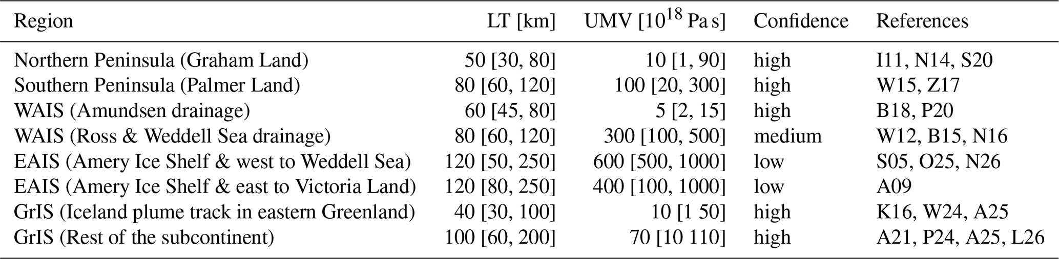
Table 1 GIA model- and data-based estimates of lithosphere thickness (LT) and upper mantle viscosity (UMV) relevant for centennial-scale solid Earth response to ice mass changes in Antarctica and Greenland. For each parameter, we provide our recommended values alongside plausible limiting values. See Fig. C1 for the region definition. References: Amalvict et al. (2009) (A09), Adhikari et al. (2021) (A21), Ajourlou et al. (2025) (A25), Bradley et al. (2015) (B15), Barletta et al. (2018) (B18), Ivins et al. (2011) (I11), Khan et al. (2016) (K16), Lewright et al. (2026) (L26), Nield et al. (2014) (N14), Nield et al. (2016) (N16), () (N26), Okuno et al. (2025) (O25), Powell et al. (2020) (P20), Pan et al. (2024) (P24), Scheinert et al. (2006) (S06), Samrat et al. (2020) (S20), Whitehouse et al. (2012) (W12), Wolstencroft et al. (2015) (W15), Weerdesteijn and Conrad (2024) (W24), Zhao et al. (2017) (Z17).

Regional estimates of lithosphere thickness (in the sense of mechanical strength used in GRD models) and mantle viscosity have considerable reliance on GNSS trends determined since the mid-to-late 2000s. However, these estimates remain ambiguous, primarily due to uncertainty in the load history (Whitehouse, 2018). When loading chronologies are well-constrained, bounds on upper mantle viscosity η can be established. Despite this, uncertainties typically remain on the order of log η±0.5 (e.g., Nield et al., 2014; Barletta et al., 2018; Adhikari et al., 2021). This ambiguity is particularly pronounced in regions characterized by low upper mantle viscosity (log η≤19.5), which are generally associated with slow seismic velocities or relatively young (Neogene) tectonic settings. In these regions, model solutions become highly sensitive to decadal to centennial-scale changes in ice mass load. Under such conditions, the framework proposed here offers particular value by capturing significant solid Earth feedback and enabling efficient exploration of parameter space and uncertainty quantification.

Observational constraints on lithosphere thickness and mantle viscosity from geodetic data are strongest in the Antarctic Peninsula and West Antarctica, whereas substantial uncertainties remain along the sparsely sampled coasts of East Antarctica. Existing constraints are geographically clustered, with studies concentrated in regions such as Graham Land (Nield et al., 2014; Samrat et al., 2020) and the South Shetland Islands (Simms et al., 2012) in the northern Peninsula, Palmer Land (Wolstencroft et al., 2015; Zhao et al., 2017), and key sectors of West Antarctica, including the Amundsen Sea Embayment (Barletta et al., 2018; Powell et al., 2020), Siple Coast (Nield et al., 2016), and the Weddell Sea Embayment (Bradley et al., 2015; Wolstencroft et al., 2015). In contrast, along the extensive East Antarctic coastline, observations are limited to a few regions, such as Dronning Maud Land (Scheinert et al., 2006; Okuno et al., 2025) and the Wilkes Subglacial Embayment (Amalvict et al., 2009), leaving the underlying solid Earth structure comparatively poorly constrained. The extensive coastline from the Amery Basin to George V Coast (spanning 90° in latitude) has an especially acute data shortage (e.g., Scheinert et al., 2026). Across these regions, studies often yield differing estimates of lithosphere thickness and upper mantle viscosity. For example, on the northern Peninsula, some studies suggest weak sensitivity to lithosphere thickness, whereas others infer a thicker lithosphere, yielding comparable viscosity values (Nield et al., 2014; Samrat et al., 2020). Given these discrepancies, prescribing a single, definitive set of regional parameters that accounts for all observations remains challenging. Here, we propose representative parameter sets informed by these studies, as our goal is not to reconcile or discount prior estimates but to provide first-order guidance to ice sheet modelers to enable coupled simulations. Accordingly, we define six sets of solid Earth parameters for Antarctica (Table 1), comprising two regional configurations each for West Antarctica, East Antarctica, and the Peninsula (Fig. C1).

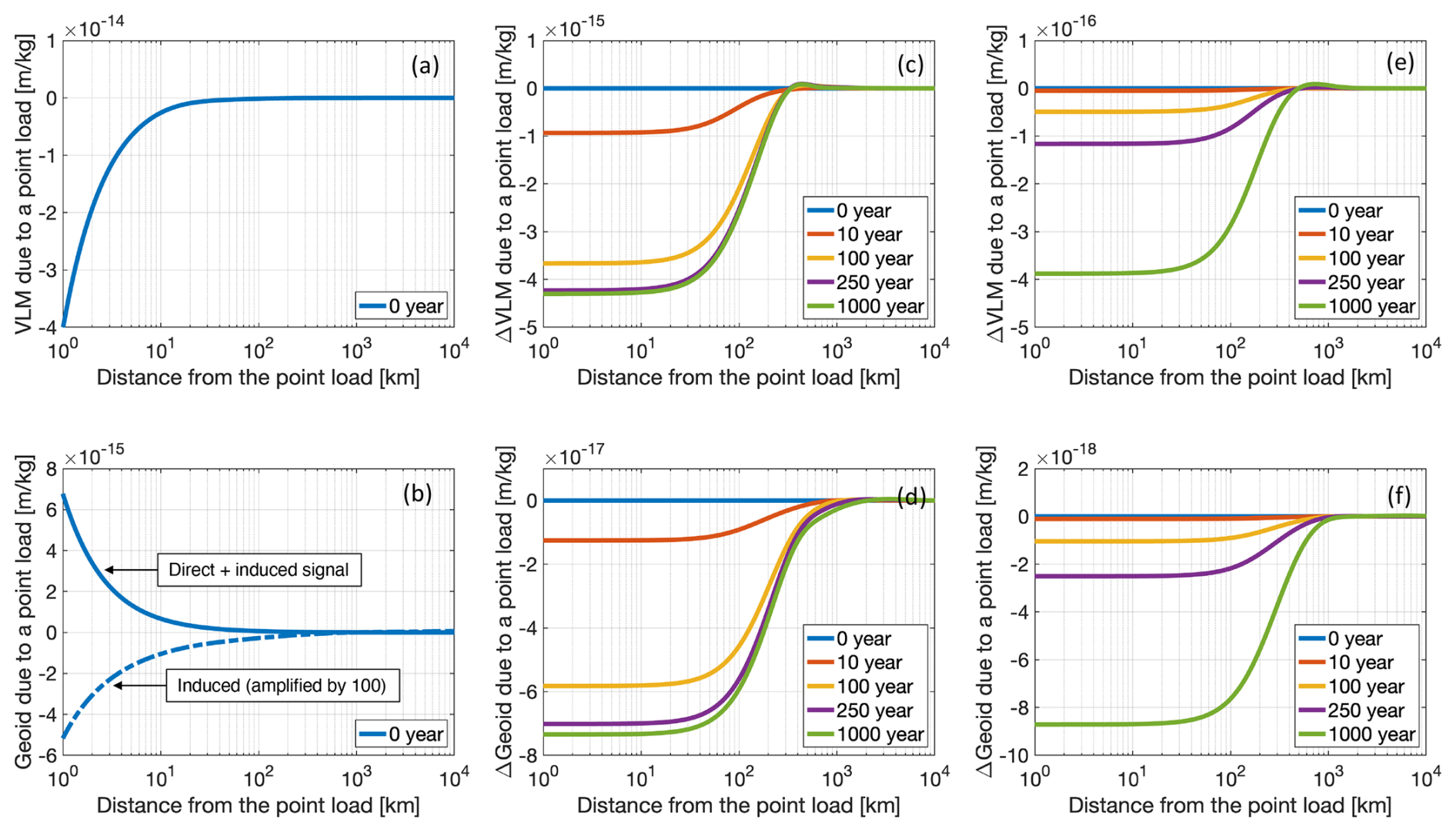
Figure 2 Time-dependent Green's functions for vertical land motion (VLM) and geoid. Panels (a, b) show the elastic signals. The direct loading effect (i.e., the first term on the right-hand side of Eq. A2) dominates the geoid signal, as the induced solid Earth response is approximately two orders of magnitude smaller and of opposite sign (panel b). Viscous signals, derived here by subtracting the elastic (panels a, b) from the total viscoelastic solutions, are shown for two contrasting earth models: (c, d) WAIS-earth and (e, f) EAIS-earth. WAIS-earth represents the viscosity structure beneath the Amundsen Sea Embayment featuring relatively thin lithosphere (60 km) and low upper mantle viscosity (5×10¹⁸ Pa s). EAIS-earth mimics a plausible structure beneath the East Antarctic coast, with a much thicker lithosphere (120 km) and a higher mantle viscosity (5×10²⁰ Pa s). In both cases, the lower mantle viscosity is fixed at 2×10²² Pa s.

As listed in the table, upper mantle viscosity spans about three orders of magnitude. Figure 2 shows Green’s functions for two contrasting Earth structures relevant for marine ice sheet modeling. The Amundsen Sea Embayment, in the West Antarctic Ice Sheet (WAIS), has a thin lithosphere (60 km) and low mantle viscosity (5×10¹⁸ Pa s). In contrast, the East Antarctic Ice Sheet (EAIS) coasts have a much thicker lithosphere (120 km) and higher viscosity (5×10²⁰ Pa s). These differences produce distinctly different responses. In the first model (WAIS-earth), the solid Earth approaches isostatic equilibrium within 250–300 years, with viscous deformation evident in less than a decade. In the East Antarctic model (EAIS-earth), noticeable relaxation develops only after about 100 years of loading.

At the other pole, the Greenland Ice Sheet (GrIS) has received comparatively less attention regarding solid Earth coupling in centennial-scale projections. Here, we provide a brief synthesis of the current state of knowledge of solid Earth structure and parameters, along with a set of recommendations (see Table 1). The data set constraining GIA in Greenland is far more extensive than those for Antarctica (e.g., Khan et al., 2016; Gowan, 2023; Berg et al., 2024; Ajourlou et al., 2025). Seismic imaging reveals three-dimensional variability of lithosphere thickness and mantle viscosity (Milne et al., 2018; Ajourlou et al., 2024), although such structure is generally localized along the Iceland plume track (Khan et al., 2016; Weerdesteijn and Conrad, 2024; Ajourlou et al., 2025). Based on these observations, we recommend adopting two sets of parameters: one for the region impacted by the plume track and the other for the rest of the subcontinent. This distinction is particularly important for accurately modeling major glaciers in central east Greenland, such as Helheim and Kangerdlugssuaq.

Recent efforts to reconcile paleo constraints with modern GNSS observations in regions minimally affected by the Icelandic plume (i.e., most of the subcontinent) support a centennial-scale mantle viscosity on the order of 5×10¹⁹ Pa s (Adhikari et al., 2021; Lewright et al., 2026). However, constraints on lithosphere thickness remain less well resolved. The inferred viscosity is typically an order of magnitude lower than values commonly adopted in GIA studies targeting millennial timescales (Lecavalier et al., 2014; Milne et al., 2018; Ajourlou et al., 2025). A broadband rheological framework with time-variable viscosity has been proposed to reconcile these differences in viscosity (Paxman et al., 2023), although further investigation is needed to determine its necessity (Pan et al., 2024). For spatial guidance, maps delineating the extent of the plume track region are provided in Khan et al. (2016) and Weerdesteijn and Conrad (2024). Within this area (Fig. C1), we recommend adopting reduced lithosphere thickness and mantle viscosity values, similar to those in the northern Antarctic Peninsula (Table 1).

4 Accuracy of the Proposed Method

We validate the proposed method by comparing example GRD results against self-consistent solutions acquired from simulating the Ice-sheet and Sea-level System Model (ISSM;  Adhikari et al., 2016; Houriez et al., 2025). In the latter, self-consistency is sought in the ocean loading and GRD solutions for a given ice loading. We accomplish this by solving the sea level equation (Farrell and Clark, 1976; Milne and Mitrovica, 1998; Kendall et al., 2005; Spada and Melini, 2019) on an unstructured Earth's surface mesh that conserves the total mass of ice and ocean. No regional model, including ours, can resolve self-consistency in global surface loading and the solid Earth response. The critical question is how well the regional model reproduces the self-consistent solutions. For identical representation of ice loading and solid Earth in the regional and global self-consistent models, the difference in predicted GRD solutions stems from the treatment of ocean loading and the rotational feedback. Here, we aim to quantify this difference for the predicted change in VLM and geoid. All regional model solutions include only the ice loading effect. In regions with grounding line migration, we consider only ice above flotation when calculating the load. Rotational feedback is also not accounted for, as shown to be negligible by Larour et al. (2019).

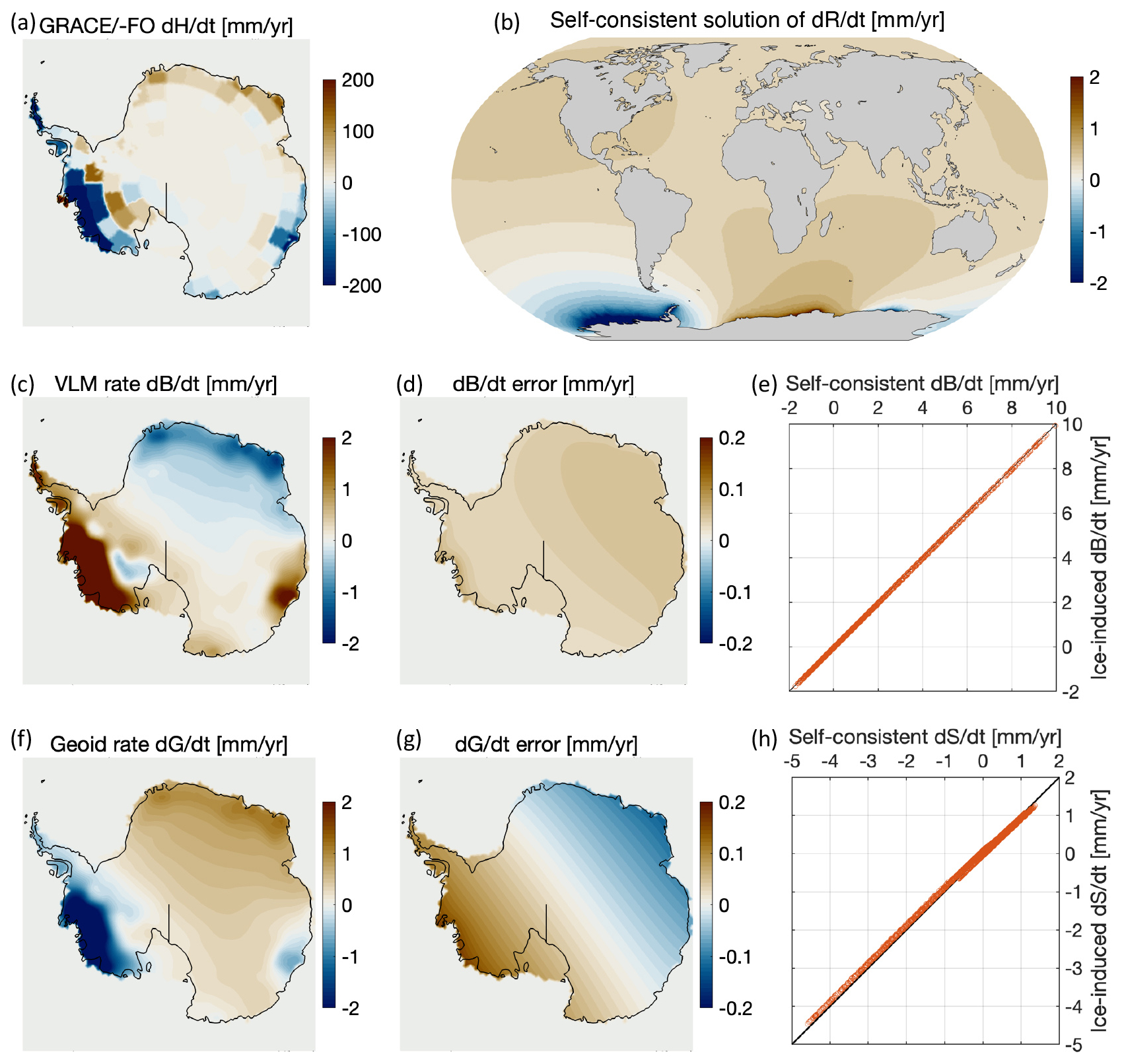
Figure 3 Method accuracy for elastic Earth models. We force the solid Earth by the observed ice load, $\mathrm{d}H/\mathrm{d}t$, derived from the Gravity Recovery and Climate Experiment (GRACE) and its Follow On (FO) mission data over 2002–2024 (a). We quantify the associated self-consistent ocean load, $\mathrm{d}R/\mathrm{d}t$, by solving the sea level equation (b). We use the self-consistent solutions (not shown) for the bedrock topography and geoid change – that capture both the ice and global self-consistent ocean loads (panels a–b) – to validate the proposed method. (c) Our estimate of vertical land motion (VLM) rate, $\mathrm{d}B/\mathrm{d}t$, induced by the ice load alone (panel a). (d) The difference in VLM rate between the self-consistent solution and the regional solution over the Antarctic domain (shown in panel c). It is at least an order of magnitude smaller than the signal, especially in regions with larger displacement. Indeed, the two solutions appear virtually the same within the ice sheet domain (e), confirming the validity of the proposed method. (f)–(h) The same as panels (c)–(e), but for the rate of change in geoid, $\mathrm{d}G/\mathrm{d}t$.

First, we examine the elastic Earth response to the observed trend in Antarctic ice mass change derived from the Gravity Recovery and Climate Experiment (GRACE) and its Follow On (FO) mission data. A key aspect of the load model is the significant mass loss occurring in the Amundsen Sea Sector and Wilkes Land, contrasted by a moderate mass gain in Dronning Maud Land (Fig. 3a). This pattern is also evident in the near field of self-consistent ocean loading (Fig. 3b), where there is a reduction in ocean load (equivalently, relative sea level) near the areas of ice loss and an increase in ocean load near the areas of ice gain. The predicted VLM and geoid fields show minor differences between the regional and global models, suggesting sufficient accuracy of the proposed method. Self-consistent VLM solution is systematically larger (Fig. 3d) due to the reinforcing effect of the ocean load, but this is insignificant in this case of a small sea level change (Fig. 3e). A similarly minor difference is observed in the geoid field (Fig. 3h). This discrepancy appears to be primarily driven by Earth’s rotational response, as evidenced by the pronounced degree-2, order-1 pattern in Fig. 3g.

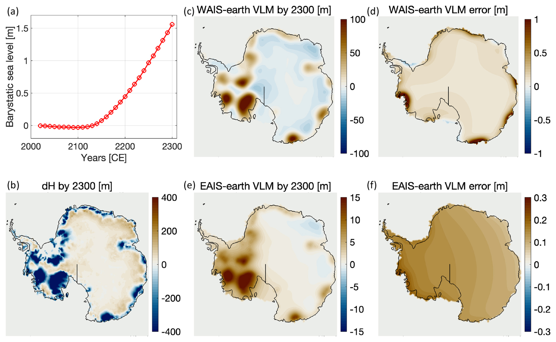
Figure 4 Method accuracy for viscoelastic Earth models. We use the evolving ice thickness data for 2010–2300 based on a solution that applied climate forcings from the recent Ice Sheet Model Intercomparison Project (ISMIP6) (Seroussi et al., 2024) to a coupled model of ice sheet, solid Earth, and sea level (Han et al., 2025): (a) Barystatic sea level change at 10-year intervals between 2010 and 2300, and (b) the cumulative changes in (thickness equivalent) ice load, dH, over 290 years. (c) Total vertical land motion (VLM) by 2300 due to ice load alone, calculated for WAIS-earth using the proposed method. (d) Difference between the self-consistent solution (not shown) and the one shown in panel (c). (e)–(f) Same as panels (c-d), but for EAIS-earth. Regardless of Earth models, VLM errors are about two orders of magnitude smaller than the signals, especially in regions with larger displacement. Geoid fields are shown in Fig. C2. Corresponding results for year 2150 are provided in Fig. C3.

Next, we evaluate the proposed method for two viscoelastic Earth models using a sample of the future evolution of the Antarctic Ice Sheet until 2300. We use precomputed ice sheet model solutions – “experiment 05” of ISMIP6 Antarctica 2300 projections under the Shared Socioeconomic Pathway SSP5-8.5 based on the UKESM climate model (Seroussi et al., 2024; Han et al., 2025) – and load the solid Earth every 10 years between 2010 and 2300 CE. In this load model, the ice sheet mass change does not contribute much to barystatic sea level during the first half of the analysis period (Fig. 4a). The sea level contribution increases rapidly after around 2150, reaching a total change of about 1.5 m. The cumulative ice thickness change suggests substantial mass loss from West Antarctica and along the coastal regions of East Antarctica (Fig.  4b). In contrast, the inland areas of the ice sheet achieve a modest mass gain.

As introduced in the previous section, we consider two Earth models representing plausible structures beneath the Amundsen Sea Embayment (WAIS-earth) and the East Antarctic coasts (EAIS-earth). In the WAIS-earth case, the predicted VLM field exhibits significantly larger amplitudes and more pronounced high wave number features (Fig. 4c) than those in the EAIS-earth case (Fig. 4e). In contrast, the EAIS-earth model yields slightly larger geoid amplitudes (Fig. C2). This difference arises because the geoid signal is primarily governed by the direct effect of surface loads, while the induced solid Earth signal is orders of magnitude smaller (see Fig. 2). Accordingly, the larger amplitudes in the EAIS-earth case reflect reduced solid Earth compensation of the gravitational potential directly associated with the imposed loading (the same for both models). Discrepancies between regional and global model solutions are small (a few percent) for both VLM and geoid fields across all considered solid Earth models. These relative differences remain consistently small over the evaluation period, as illustrated for years 2150 (Fig. C3) and 2300 (Figs. 4 and C2). These differences tend to be larger in regions of strong mass loss and associated bedrock uplift and geoid change. Overall, they primarily reflect the generally reinforcing effect – particularly at long wavelengths – of processes omitted in the regional models, especially ocean loading.

Last, we examine coupled ice/Earth simulations for Thwaites Glacier, building on a recent study by Houriez et al. (2025), to assess the utility of our proposed method in simulating ice sheet dynamics. Their approach uses an anisotropic mesh to capture kilometer-scale grounding line migration and allows for a coupling interval as short as one year. The ice sheet model is initialized by optimizing basal friction and ice rheology to match observed surface velocity (Rignot et al., 2014). It handles basal melt via the PICOP parameterization (Pelle et al., 2019). This approach relies on simulating buoyant plume-driven sub-shelf meltwater circulation within the Potsdam Ice-shelf Cavity Model (PICO) framework (Reese et al., 2018). Model inputs for ocean temperature, salinity, and surface mass balance are based on the Community Earth System Model (CESM) SSP5-8.5 scenario (Danabasoglu et al., 2020). The Earth model complies with the Maxwellian structure constrained by GNSS data (Barletta et al., 2018) and further considers a transient relaxation of the asthenosphere and upper mantle based on the laboratory experiments, the results of which are couched in the formalism of the extended Burgers material (EBM) model (Faul and Jackson, 2015; Ivins et al., 2023a). See Fig. C4 for the characteristic signals of the solid Earth model.

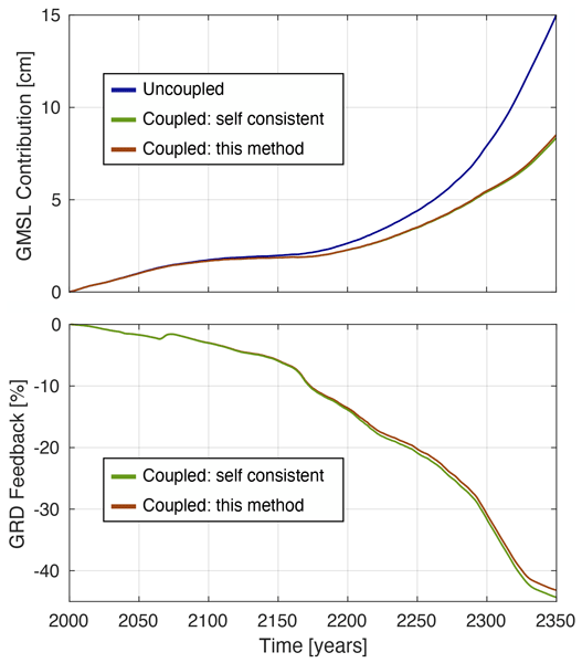
Figure 5 shows predicted grounding line positions and barystatic contributions from a standalone ice sheet simulation and two coupled simulations: one captures the ocean loading effect and rotational feedback (i.e., self-consistent solution), and the other does not (equivalently, the proposed method). The latter coupled model excellently reproduces the self-consistent solutions, capturing the GRD effect on barystatic sea level within 1 % for most of the time. This discrepancy increases up to 2 % by the end of the simulation as a viscous response to ocean loading accumulates over time. It is insignificant compared to the large disparity in the centennial-timescale projections of the Antarctic Ice Sheet (Seroussi et al., 2024). Despite its overall strong performance, we caution that our regional model may exhibit small but potentially important local deviations from those reported here. Even kilometer-scale offsets in grounding line position near bedrock ridges can influence the timing of unpinning and subsequent ice sheet retreat by several years (e.g., Larour et al., 2019; Houriez et al., 2025).

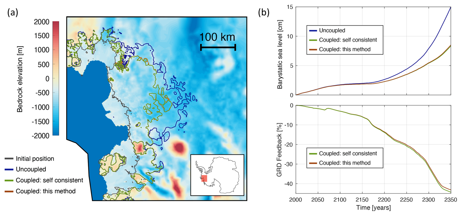
Figure 5 Method accuracy for coupled simulations. We leverage high-resolution coupled simulations for 2000–2350 that try to find consistency in ice sheet dynamics (hence, ice loads), Earth's gravitational, rotational, and deformational (GRD) response, and ocean mass distribution (Houriez et al., 2025). We reproduce key diagnostics of such simulations by coupling the ice sheet and solid Earth with the exclusion of ocean loads and rotational feedback. (a) Predicted grounding line positions at 2350 for standalone (uncoupled) ice sheet model and two coupled simulations. (b) Barystatic sea level and GRD feedback captured in coupled simulations.

These examples demonstrate our method's excellent ability to capturing self-consistent solutions within the ice sheet domain. We show that the predicted VLM and geoid fields and their impact on ice dynamics on decadal to centennial timescales are primarily influenced by the direct ice load, which the proposed method can easily handle. The impacts of ocean load and rotational feedback are minimal, although our method can still capture some of these signals. For instance, the ocean load near the ice sheet may be derived and refined iteratively from the VLM and geoid fields, as in the classical sea level solver. However, refined ocean loads may not perfectly align with the self-consistent solutions. Additionally, the centrifugal potential perturbed by ice (and near-field ocean) and its effect on VLM and geoid fields can be computed semi-analytically. Since the ice load alone captures most of the near-field signals with sufficient accuracy – and given that our primary focus in this paper is on the straightforward retrieval of the leading-order solid Earth signals within the ice sheet model domains – we do not recommend pursuing these higher-order signals, as it may require a more complex workflow for a minimal gain in solution accuracy.

5 Conclusions

We propose a straightforward method that enables ice sheet models to capture realistic solid Earth feedback on decadal to centennial timescales. This method only involves interpolating precomputed Green's functions and performing matrix multiplication with the evolving ice loading. Consequently, it introduces no numerical complexity and does not significantly increase computational costs for ice sheet models. We demonstrate that this method reproduces self-consistent solutions for time-dependent geoid and bedrock topography fields within the ice sheet domain. When the objective is to simplify the ice/Earth coupling strategy while retaining the leading feedback on centennial timescales, we show that ocean loading effects (driven by local or far-field ice mass loss or migrating coastlines) and rotational feedback can be neglected. However, in applications where these processes are essential – such as global glacial isostatic adjustment modeling or interhemispheric ice-sheet interactions – a fully self-consistent solution of the sea level equation remains indispensable (Farrell and Clark, 1976; Milne and Mitrovica, 1998). Our method should therefore not be interpreted as a substitute for a sea level solver.

Recent studies highlight the high sensitivity of solid Earth feedback to ice sheet model resolution and coupling time intervals (e.g., Han et al., 2022; Wan et al., 2022; Houriez et al., 2025; Kodama et al., 2025). In coupled simulations involving a global sea level solver, frequently capturing kilometer-scale features, such as subtle migrations of grounding lines and evolving bedrock ridges, can be challenging. In contrast, our approach – despite the noted limitations – allows ice sheet models to determine the spatiotemporal resolution of solid Earth response signals without added complexity or computational costs. This simplified framework provides a more accessible pathway for ice sheet modelers, including those using standalone systems with limited resources or expertise in solid Earth processes, to incorporate a reasonably accurate ice/Earth feedback without significant overhead. Moreover, this reduced-complexity approach enables shorter coupling intervals, yielding more realistic (in certain respects) ice-sheet evolution and projections, or alternatively supports larger ensemble simulations, thereby improving uncertainty quantification and offering a practical advantage for probabilistic sea level projections.

The core idea of our method is to leverage precomputed Green’s functions for a radially stratified solid Earth. Open-access tools are available to compute Love numbers and Green’s functions for a range of linear viscoelastic models such as Maxwell, Burgers, or extended Burgers materials (e.g., Spada et al., 2004; Caron et al., 2026). An extensive collection of Green’s functions for Maxwellian Earth models is already available (Adhikari and Caron, 2024). This library spans a wide range of plausible solid Earth structures, from models with a thin lithosphere and relatively weak upper mantle – such as those inferred geodetically beneath the Amundsen Sea Embayment or the northern Antarctic Peninsula (e.g., Nield et al., 2014; Barletta et al., 2018), as well as from seismic constraints in the Wilkes and Aurora Subglacial Basins (Hansen and Emry, 2025) – to models with cratonic lithosphere and a comparatively stiff mantle, as commonly adopted in glacial isostatic adjustment studies (Lecavalier et al., 2014; Whitehouse, 2018). We aim to further extend this library by performing additional computations for more refined Earth structures, including explicit asthenosphere layering, and more general linear viscoelastic formulations that incorporate transient rheology. Such extensions may be important for accurately modeling ice/Earth feedback at drainage basin scales.

Appendix A: Love Numbers and Green's Functions

The gravitational and deformational response of the solid Earth to a point load applied at its surface is commonly known as the loading Love numbers. These Love numbers play a crucial role in loading studies, including glacial isostatic adjustment theory, under the assumption of radial Earth symmetry. They are derived from the so-called y_i system of equations based on the principles of mass conservation, momentum conservation, and Poisson's equation (Alterman et al., 1959; Peltier, 1974). Here, we leverage the recently coded Love number capability (Caron et al., 2026) of the Ice-sheet and Sea-level System Model (ISSM) that solves the y_i system in the Laplace domain for a suite of linear viscoelastic rheologies, including compressible elastic, Maxwell, Burgers, and extended Burgers materials. It employs the Post-Widder method to convert the spectral solutions to the time domain (Spada and Boschi, 2006). The code has been optimized for parallel performance at high spherical harmonic degrees, targeting to resolve kilometer-scale processes critical for understanding ice sheet and solid Earth interactions (Larour et al., 2019; Houriez et al., 2025). It has been validated against community standards (Spada et al., 2011). The Love numbers related to radial deformation, h_n(t), and gravitational potential, k_n(t), are particularly relevant here. Figure A1 shows example Love numbers for two models representing the solid Earth beneath West and East Antarctica (also see Fig. 2).

Time dependent Love numbers can be assembled to derive the displacement and geoid response to the surface point load (Longman, 1962; Farrell, 1972). These response functions, called Green's functions, may be written as follows:

$$\begin{array}{}\text{(A1)}& {\displaystyle }{K}_{\mathrm{B}}(\mathit{\alpha },t)& {\displaystyle }=D\sum _{n=\mathrm{0}}^{\mathrm{\infty }}{h}_{\mathrm{n}}\left(t\right){\mathcal{P}}_n\left(\cos \mathit{\alpha }\right),\text{(A2)}& {\displaystyle }{K}_{\mathrm{G}}(\mathit{\alpha },t)& {\displaystyle }=D\sum _{n=\mathrm{0}}^{\mathrm{\infty }}\left[\mathrm{1}+k_{\mathrm{n}}\left(t\right)\right]{\mathcal{P}}_n\left(\cos \mathit{\alpha }\right).\end{array}$$

Here K_B and K_G are Green's functions for bedrock motion (VLM) and geoid, 𝒫_n are Legendre polynomials of degree n, α is the arc length between the location of point load and the location at which the solid Earth response is evaluated (see Sect. 2), and $D=\mathrm{3}/\left(\mathrm{4}\mathit{\pi }{r}^{\mathrm{2}}{\mathit{\rho }}_{\mathrm{e}}\right)$ is the dimensioning constant with ρ_e denoting the mean Earth density. Note that the unity term appearing in the brackets of Eq. (A2) represents the direct effect of the point load on the geoid signal, whereas Love numbers k_n characterize the induced solid Earth response.

We may evaluate the infinite sum in the above equations by truncating the series at a sufficiently high degree, say at n=N. A truncation at N=10⁴ may be sufficient to capture high wave-number features, such as subtle migration of grounding lines or uplift of subglacial mountains and ridges, critical for understanding the ice/Earth feedback mechanisms (Houriez et al., 2025). However, it appears insufficient to yield accurate and smooth Green's functions, especially in the near field of the loading point (Fig. A2). Noting the asymptotic nature of h_n(t)→h_∞ and nk_n(t)→k_∞ as n→∞ (see Fig. A1), Farrell (1972) suggests employing the so-called Kummer's transformation to get rid of these noises. For a sufficiently high-degree truncation, we may invoke h_∞≈h_N and k_∞≈Nk_N and express Green's functions as follows:

$$\begin{array}{}\text{(A3)}& {\displaystyle }{K}_{\mathrm{B}}(\mathit{\alpha },t)\approx D\left\{{\displaystyle \frac{h_{\mathrm{\infty }}}{\mathrm{2}\sin (\mathit{\alpha }/\mathrm{2})}}+\sum _{n=\mathrm{0}}^N\left[h_{\mathrm{n}}\right(t)-h_{\mathrm{\infty }}]{\mathcal{P}}_n\left(\cos \mathit{\alpha }\right)\right\},\text{(A4)}& {\displaystyle }\begin{array}{rl}{K}_{\mathrm{G}}(\mathit{\alpha },t)& \approx D\left\{{\displaystyle \frac{\mathrm{1}}{\mathrm{2}\sin (\mathit{\alpha }/\mathrm{2})}}-k_{\mathrm{\infty }}\ln \left[\mathrm{2}\sin \left({\displaystyle \frac{\mathit{\alpha }}{\mathrm{2}}}\right)\right]\right.\\ & \left.+\sum _{n=\mathrm{1}}^N\left[k_{\mathrm{n}}\right(t)-{\displaystyle \frac{k_{\mathrm{\infty }}}{n}}]{\mathcal{P}}_n\left(\cos \mathit{\alpha }\right)\right\}.\end{array}\end{array}$$

As shown in Fig. A2, these expressions behave smoothly and are free from oscillatory artifacts. Adhikari and Caron (2024) deliver such solutions of Green's functions and corresponding Love numbers for numerous Maxwellian Earth models (Sect. 3). Wide spatiotemporal domains and sufficiently dense sampling of these signals across a broad range of radially symmetric Earth structures will enable high-resolution coupled ice/Earth simulations on centennial timescales.

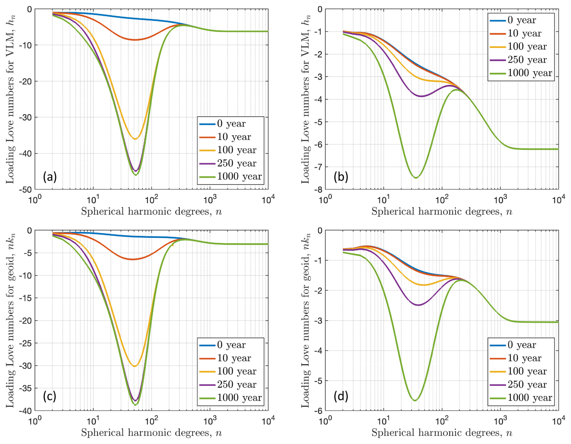
Figure A1 Viscoelastic Love numbers. We show example solutions for two Earth models introduced in Fig. 2: WAIS-earth (left panels) and EAIS-earth (right panels). Love numbers h_n (upper panels) and k_n (lower panels) are relevant for vertical land motion (VLM) and geoid estimation, respectively. Note the asymptotic nature of h_n(t) and nk_n(t) towards their respective constants h_∞ and k_∞ as n→∞. These constants solely depend on the elastic structure of the Earth. For the preliminary reference Earth model (Dziewonski and Anderson, 1981), we find $h_{\mathrm{\infty }}\approx h_{\mathrm{10},\mathrm{000}}=-\mathrm{6.214}$ and $k_{\mathrm{\infty }}\approx {\mathrm{10}}^{\mathrm{4}}{k}_{\mathrm{10},\mathrm{000}}=-\mathrm{3.055}$. Notice the different y-axis limits, highlighting the contrasting response signals for the two Earth models. The low viscosity regime in WAIS-earth yields larger-amplitude viscous signals. The thinner lithosphere in this model implies a significant viscous response at high wave numbers (n≈300 as opposed to n≈200 in EAIS-earth).

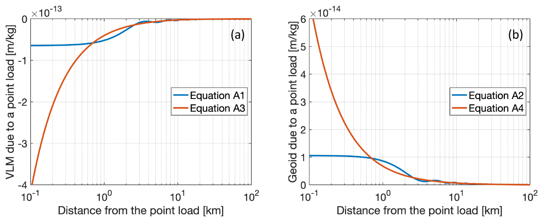
Figure A2 Evaluation of infinite sum in Green's functions. Since evaluating Love numbers up to infinitely large degrees is impractical, we have to truncate the sum appearing in Eqs. (A1) and (A2) at a sufficiently high degree n=N. Even if we truncate the sum at N=10⁴, Green's functions oscillate in the near field of the applied point load (see blue lines). We handle these oscillations inherent to infinite sums by leveraging the asymptotic nature of Love numbers (see Fig. A1) and using the Kummer transformation that partitions Green's functions into an analytic part whose exact solution exists and the finite sum that yields zero for n≥N. The transformed expressions (Eqs. A3 and A4) accurately capture Green's functions in the near field, hitting the inherent singularity at the loading point (red lines).

Appendix B: A Strategy for Implementing the Proposed Method

Here, we summarize a strategy that may be adapted to evaluate key matrices and convolution. The example we provide is written for Matlab and shall be adapted in any language.

Distance matrix $\mathit{\alpha }(\mathit{x},{\mathit{x}}^{\prime })$:

We assume that the ice sheet mesh does not evolve in lateral dimensions, allowing us to compute the distance between the loading points (assumed to be elemental centroids) and evaluation points (assumed to be elemental vertices) only once. Let ${\mathit{x}}_k\equiv ({\mathit{\varphi }}_k,{\mathit{\lambda }}_k)$ for $k=[\mathrm{1},q]$ and ${\mathit{x}}_j^{\prime }\equiv ({\mathit{\varphi }}_j^{\prime },{\mathit{\lambda }}_j^{\prime })$ for $j\in [\mathrm{1},p]$ be the geographic coordinates (in radians) of elemental vertices and centroids. The distance matrix will be of q×p size, where q and p are the total numbers of evaluation and loading points in space (Fig. 1b). We may compute α as follows:

 for k = 1:q
    dphi = abs(phi2-phi1(k));
    dlam = abs(lambda2-lambda1(k));
    alpha(k,:) = r*2
    *asin(sqrt(sin(dphi/2).^2
    +cos(phi1(k)).*cos(phi2).
    *sin(dlam/2).^2));
 end

Green's function K_X(α,τ):

We assume that the loading time t^′ and the evaluation time t are relative to the same reference point and that their discrete representations are known apriori. It allows us to predetermine a set of unique non-negative τ, where $\mathit{\tau }=t-t^{\prime }$ (Figure 1c), and prepare Green's function matrix only once before model run.

 tau = unique(transpose(t) - t_prime);
 tau = tau(tau >= 0);

We may now load “greensfunctions.nc” (Adhikari and Caron, 2024) and extract desired solutions for the chosen solid Earth model. All non-defined variables in the following example code are the default variables in the NetCDF file. (We may need to interpolate the solutions further if the desired lithosphere thickness or mantle viscosity does not match those provided.) In this example, we only load Green's functions required for VLM estimation.

 litho_idx = find(litho_thick
 ==this_litho); % this_litho:
 user defined litho thickness [km]
 mant_idx  = find(mant_visco==this_mant);
 % this_mant: user defined mantle
 viscosity [Pa s]
 greens_h_for_desired_earth
  = squeeze(greens_function_h(litho_idx,
  mant_idx,:,:));
 greens_h_at_desired_times
 = zeros(length(dist),length(tau));
 for ii = 1:length(dist)
    greens_input
    = greens_h_for_desired_earth(:,ii);
    greens_h_at_desired_times(ii,:)
    = interp1(eval_times,greens_input,
    tau);
 end

Finally, we may prepare a three-dimensional Green's function matrix, which will be untouched throughout the coupled model simulations. The following example uses a structure with dynamic variables to access specific Green's functions during convolution easily. The structure “Gvlm” has the same number of fields as the number of τ and each field has a size of q×p, where p and q are once again the total number of elements and vertices.

 for ii = 1:length(tau)
    time_tag = ['tau',num2str(tau(ii))];
    Gvlm.(time_tag) = interp1(dist,
    greens_h_at_desired_times(:,ii),
    alpha);
 end

Loading function $\mathrm{\Delta }\mathcal{L}({\mathit{x}}^{\prime },t^{\prime })$:

Let m be the total number of Heaviside loads prior to the specific coupling time t (Figure 1c). The loading function $\mathrm{\Delta }\mathcal{L}({\mathit{x}}^{\prime },t^{\prime })$ would have a size of p×m, where p is the number of elements. The ice sheet model computes this function (in units of kg), which we refer to in the following code as ”deltaload”.

Convolution $X(\mathit{x},t)=K_X(\mathit{\alpha },\mathit{\tau })\otimes \mathrm{\Delta }\mathcal{L}({\mathit{x}}^{\prime },t^{\prime })$:

We may perform the spatiotemporal convolution and retrieve the desired GRD signal (vertical land motion “vlm,” in this example) as follows.

 vlm = zeros(q,1);
 for ii = 1:m
    tau = t - t_prime(ii);
    time_tag = ['tau',num2str(tau)];
    vlm = vlm + sum(bsxfun(@times,
    Gvlm.(time_tag),transpose
    (deltaload(:,ii))),2);
 end

Appendix C: Supporting Materials

Here, we include supporting figures (Figs. C1–C4) referenced in the main text.

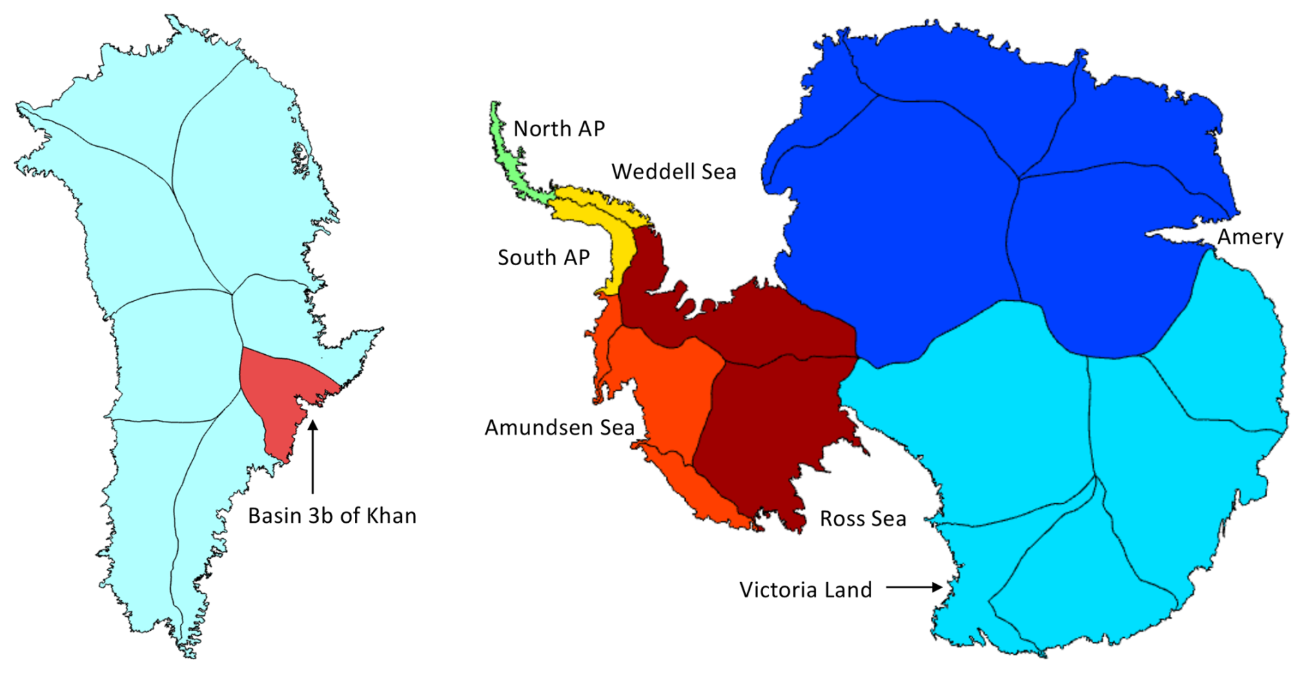
Figure C1 This figure, supplementing Table 1, shows the recommended basin boundaries with distinct solid-Earth parameters: two for Greenland and six for Antarctica. Basin delineations are from Mouginot and Rignot (2019) for Greenland and (Rignot et al., 2013) for Antarctica. The Greenland partition includes basin 3b of Khan et al. (2016), which exhibits anomalously large GNSS uplift signals indicative of the Icelandic plume-affected region.

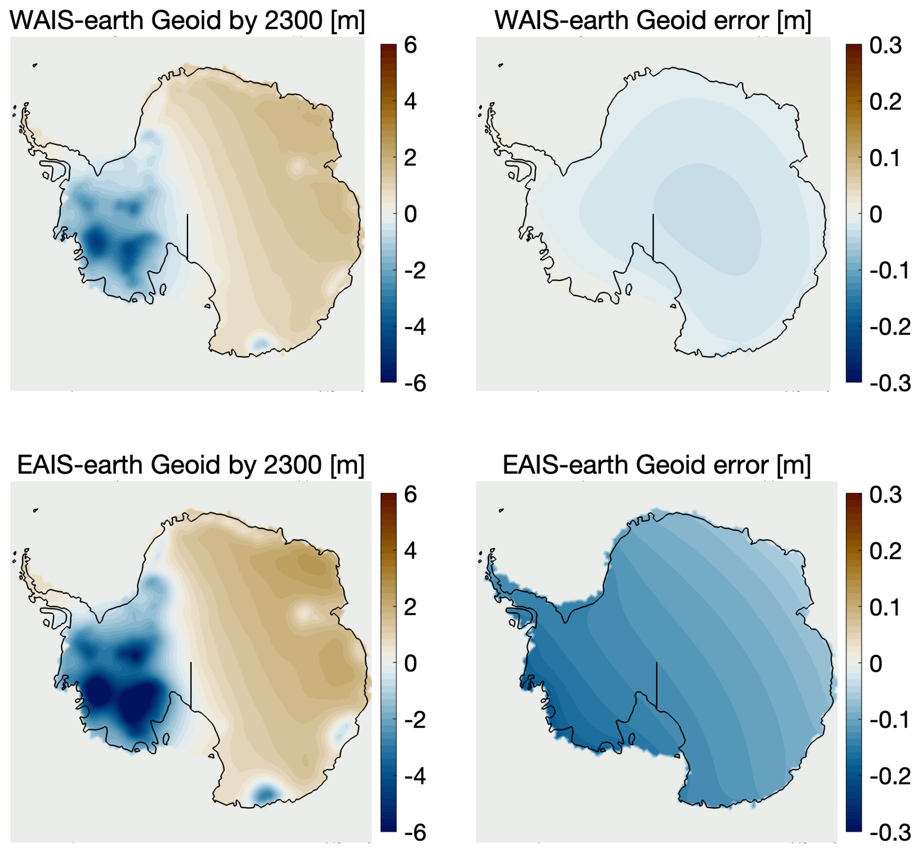
Figure C2 Supplementing Fig. 4, this figure shows geoid fields and their errors relative to self-consistent solutions. The larger amplitudes in the EAIS-earth case reflect reduced solid Earth compensation (compare Fig. 2d versus 2f) of the gravitational potential directly induced by the imposed surface loads (Fig. 2b). The enhanced errors in the EAIS-earth configuration likely arise from the relatively greater influence of direct ocean loading – absent in the regional simulations – compared to the compensating solid Earth response.

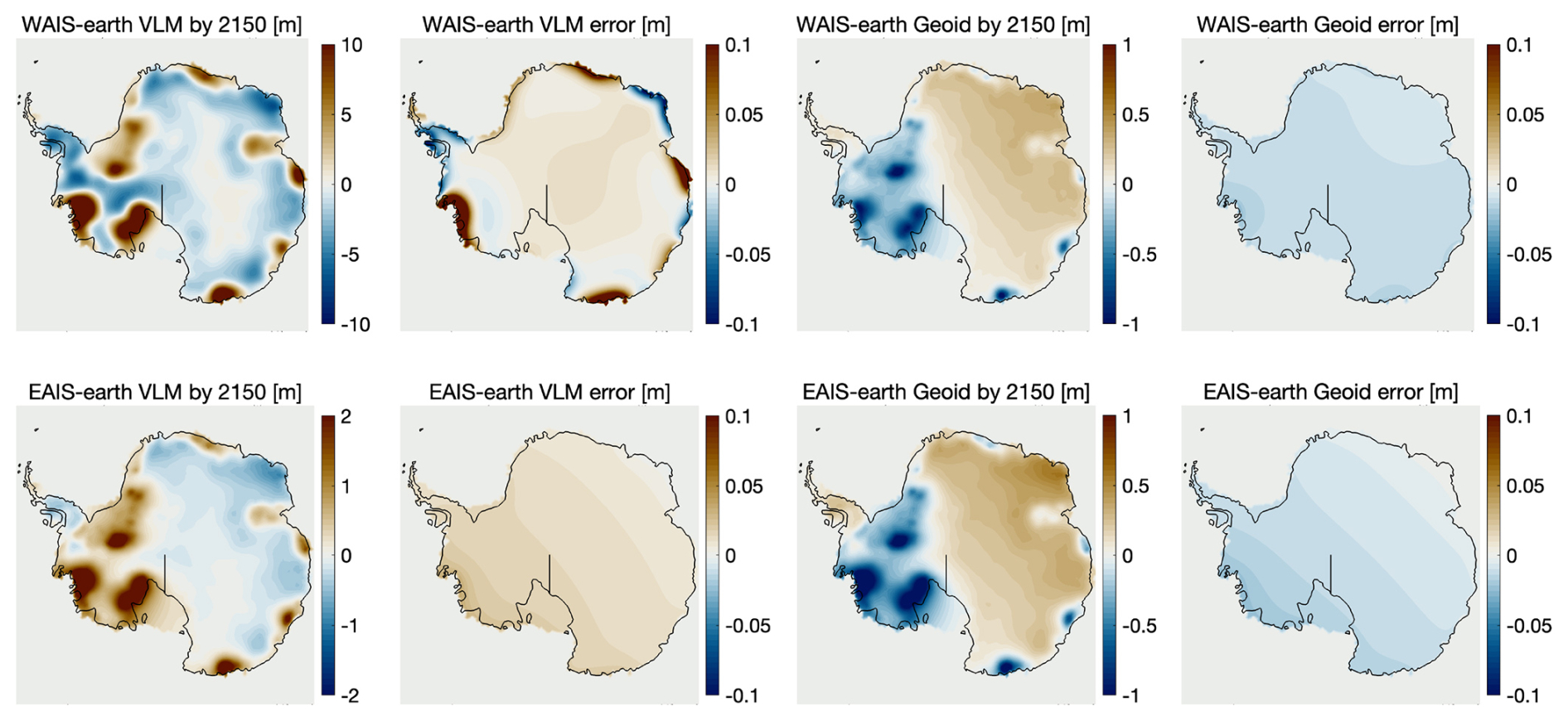
Figure C3 Supplementing Fig. 4, this figure shows VLM and geoid fields at year 2150 and their errors relative to self-consistent solutions.

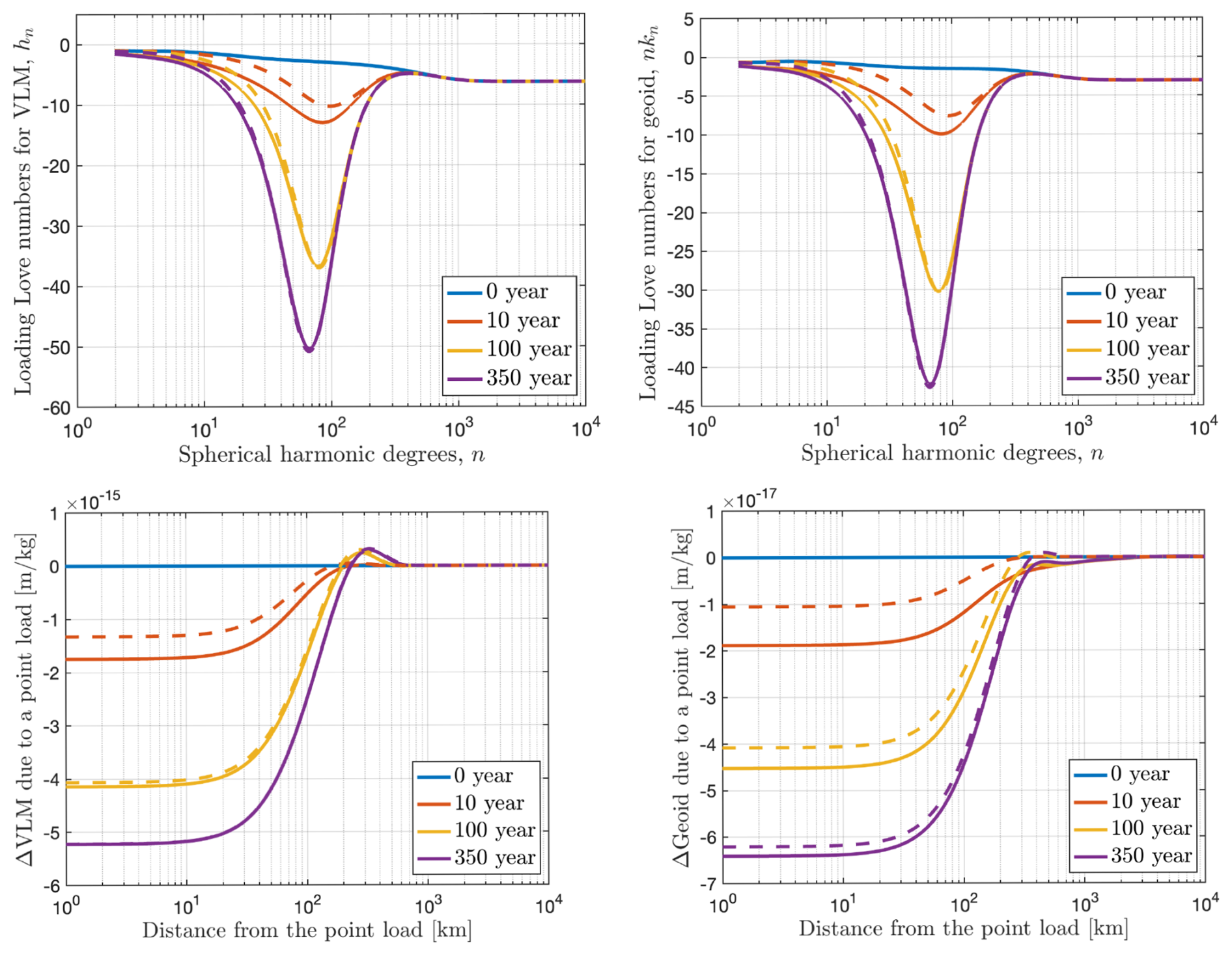
Figure C4 Love numbers and Green’s functions for the EBM model (solid lines) used in the coupled simulations (Fig. 5). The upper panels show Love numbers for VLM and geoid change, while the lower panels present the corresponding Green’s functions (viscous component). The model consists of a three-layer viscoelastic mantle beneath a 50 km thick lithosphere: a 150 km asthenosphere, an upper mantle extending from 200 to 670 km depth, and a lower mantle. The corresponding Maxwell viscosities are 3.16×10¹⁸, 2×10²⁰, and 2×10²² Pa s. EBM parameters are held constant across all layers, with Δ=3, α=0.5, τ_H=7 years, and τ_L=54 minutes, and the elastic structure follows PREM (cf. Table 2 of Houriez et al., 2025). Dashed curves denote the equivalent Maxwell model with the same viscosity structure, highlighting the enhanced transient response of the EBM at shorter timescales. It is interesting to note that the transient response has a relatively longer memory in the geoid signals (right panels) than in the VLM (left panels).