Dry snow initialization and densification over the Greenland and Antarctic ice sheets in the ORCHIDEE land surface model

Accurate modeling of the snowpack over ice sheets is essential for quantifying their surface mass balance contribution and their resulting impact on sea level rise. The snowpack evolution is largely governed by surface climate but also by internal processes such as densification. In land surface models, such processes are often represented using formulations developed for seasonal snow, limiting their realism in polar environments. To improve the representation of polar snow in the land surface model ORCHIDEE (Organizing Carbon and Hydrology in Dynamic Ecosystems), the surface component of the IPSL-CM climate model, we implement a series of developments over Greenland and Antarctica. These developments include (1) a new snowpack initialization procedure that generates deep and physically consistent density profiles based solely on latitude and elevation, which may be useful for other snowpack models, (2) a wind-based surface snow density parameterization applicable to both Greenland and Antarctica, and (3) a recalibrated dry-snow densification scheme for snowpack compaction, using observations and 1D and 2D offline simulations. These developments improve the simulation of surface snow density as well as the internal snowpack structure, including both density and temperature, with good agreement with dry-snow observations. Discrepancies still persist in representing the Greenland ablation zones, suggesting that further improvements in surface energy balance processes are needed, with specific attention to snow albedo.

1 Introduction

The evaluation of the ice sheets mass balance is crucial to understand their evolution and their potential contribution to sea-level rise (Alley et al., 2005; Box et al., 2022; Otosaka et al., 2023). In Antarctica, ice sheet mass changes are primarily driven by basal melting and ice discharge into the ocean (Rignot et al., 2019), whereas in Greenland, mass loss is dominated by surface processes (van den Broeke et al., 2016; Mouginot et al., 2019). Due to higher atmospheric temperatures and the subsequent increase in surface melt, the mass loss of the Greenland ice sheet (GrIS) has accelerated over recent decades, contributing to approximately 20 % of the observed global sea-level rise (Forsberg et al., 2017; Otosaka et al., 2023). In the Antarctic ice sheet (AIS), surface ablation is limited to specific areas mainly located in the Antarctic Peninsula and the ice shelves (Shepherd et al., 2018; Leduc-Leballeur et al., 2020). Overall, the AIS has contributed to 10 % of the observed global mean sea-level rise since 1993 (Oppenheimer et al., 2019). Under continued surface warming, the mass balance of the ice sheets is projected to further decrease, driven by enhanced surface melt, ice discharges and basal melting (Oppenheimer et al., 2019).

Surface ablation is strongly related to the processes occurring on the surface and within the snowpack overlying the ice sheet. The snowpack is a porous material composed of snow crystals, air and, potentially, liquid water. This porosity enables the retention and refreezing of surface meltwater or rainwater that percolates within the snow layers (Vandecrux et al., 2020; Amory et al., 2024). Over the GrIS, the increased surface melt and the expansion of the melt area (Mouginot et al., 2019; Mousavi et al., 2021) affect the snowpack internal properties, notably inducing an increase in ice lens formation, (de la Peña et al., 2015; Vandecrux et al., 2018), a rise in the snowpack temperature driven by an increase in meltwater percolation and refreezing (Polashenski et al., 2014; van den Broeke et al., 2016) and a decrease in pore spaces reducing the retention and refreezing of water (van Angelen et al., 2013; Vandecrux et al., 2019). These changes are closely linked to variations in snow density, a fundamental property that constrains the pore space available for meltwater retention and refreezing. As a consequence, a detailed understanding and modeling of physical processes governing densification is crucial to constrain the current and future mass changes of both ice sheets.

Different stages of dry snow densification can be distinguished, starting with the surface densification that occurs at the top of the snowpack. According to Arctic field studies, the surface density in polar regions can be related to the combined effects of wind compaction and the upward transfer of water vapor induced by the high temperature gradient within polar snowpacks (Barrere et al., 2017; Domine et al., 2016), although this latter effect is still debated (Jafari and Lehning, 2023). Moreover, frequent strong winds cause large amounts of snow to be transported, compacted, and sublimated, contributing to the denser surface layers (Liston and Sturm, 2002; Sturm et al., 2001). Recent wind tunnel experiments further quantified surface snow densification, showing that it strongly depends on wind speed and the duration of wind exposure (Walter et al., 2024). Similarly, observations during a drifting-snow event in Adélie Land revealed rapid post-depositional snow densification, with density increasing from approximately 200 to around 350 kg m⁻³ in a single day (Amory et al., 2021). Saltation also appears to be a driver of surface densification as shown by wind-tunnel experiments, emphasizing the role of particle impacts, fragmentation and sintering in enhancing snow compaction (Sommer et al., 2017). However, there is a lack of surface observations in polar regions limiting our ability to determine which processes are involved in surface densification.

Below the surface, two main dry-snow densification stages can be distinguished. The first one occurs until density reaches around 550 kg m⁻³ and is characterized by rapid compaction associated with grain settling and packing (Herron and Langway, 1980; Arnaud et al., 1998). Between 550 and 830 kg m⁻³, the densification rate declines and deformation is primarily due to viscous creep and sintering under an increasing overburden pressure (Arnaud et al., 1998). Around 830 kg m⁻³, known as the bubble close-off density, ice forms and air bubbles become trapped. Densification slows significantly as air can no longer escape, and compaction occurs by compressing the trapped air bubbles (Herron and Langway, 1980; Goujon et al., 2003; Stevens et al., 2020). Temperature and accumulation regulate the densification rate by controlling snow viscosity and mass loading, while metamorphism modifies the snow microstructure rather than driving densification itself (Arnaud et al., 1998; Goujon et al., 2003). As a result, densification can take years to centuries under cold or low accumulation conditions. This way, the interior of the ice sheets densifies slowly, whereas warmer and/or higher-accumulation regions (such as the southeastern part of the GrIS or the West AIS) densify more rapidly (van den Broeke, 2008; Ligtenberg et al., 2011; Vandecrux et al., 2020; van Kampenhout et al., 2017).

Several parameterizations have been proposed to describe snow densification. Early approaches expressed the densification rate as an Arrhenius-type function of temperature, with an additional dependence on accumulation (Herron and Langway, 1980; Barnola et al., 1991). Such parameterizations have been later refined by introducing distinct activation energies for grain growth and vapor diffusion (Arthern et al., 2010; Ligtenberg et al., 2011). This framework has been adopted in polar atmospheric models, including RACMO (Ligtenberg et al., 2011; Kuipers Munneke et al., 2008). Alternative formulations link densification directly to snow microstructural properties, such as grain size and shape (Alley, 1987; Arnaud et al., 1998; Goujon et al., 2003). Other models represent the change in snow density as a function of snow viscosity, inspired by the formulation proposed by Anderson (1976), later implemented and adapted in ISBA-ES (Decharme et al., 2016), ORCHIDEE (Wang et al., 2013; Charbit et al., 2024), CROCUS (Vionnet et al., 2012), and CESM (van Kampenhout et al., 2017). In these models, viscosity is expressed as a function of density and temperature. In more advanced schemes, viscosity also depends on the liquid water content (Decharme et al., 2016) and microstructure properties such as grain diameter and shape (Bartelt and Lehning, 2002; Steger et al., 2017; Vionnet et al., 2012).

Since many densification rate schemes rely on the physical constraint imposed by the snow mass, their performance is sensitive to how the snowpack thickness is initialized. In Greenland and Antarctica, the ice sheet snowpack can reach several tens of meters (Amory et al., 2024), and can locally exceed 100 m, like at the South Pole where snow densification occurs at a slow rate (van den Broeke, 2008). To form a thick snowpack over polar regions, many models such as ORCHIDEE, CESM, SNOWPACK and IMAU-FDM therefore rely on a spin-up procedure where the snowpack is built through natural accumulation from a snow-free state. Under the assumption of climatic stationarity, this process can take decades to over a century, depending on the local accumulation rate (Charbit et al., 2024; van Kampenhout et al., 2017; Ligtenberg et al., 2011; Keenan et al., 2021; Veldhuijsen et al., 2023). While widely used, such approaches are time-consuming and highlight the need for standardized, physically consistent, and efficient methods to better constrain the initial state of the ice sheet snowpack.

In this study, we evaluate and improve the capacity of the ORCHIDEE (Organising Carbon and Hydrology in Dynamic Ecosystems) land surface model (Krinner et al., 2005) of the IPSL (Institut Pierre Simon Laplace) Earth System Model (ESM) (Boucher et al., 2020; Cheruy et al., 2020), to represent snow densification processes over GrIS and AIS. To this end, in Sect. 3, we develop and test (1) a new automatic initialization method for Antarctica and Greenland snowpacks, generalizable to every snowpack model, (2) a new surface snow density parameterization, common for both ice sheets, and finally (3) a recalibration of the ORCHIDEE densification scheme using the History Matching (HM) method (Williamson et al., 2013), applied to 1D simulations at two reference sites. In Sect. 5, we then evaluate the calibrated and updated model in 2D offline configurations using observed density profiles across both ice sheets. Finally, we study the impact of these developments on the snowpack and its internal characteristics, such as snow temperature, liquid water retention and refreezing (Sect. 6).

2 Data and modeling setup

2.1 The Explicit Snow module over ice sheets in the ORCHIDEE land surface model

The ORCHIDEE model is the terrestrial component of the IPSL ESM. It simulates the water, carbon and energy exchanges between the land surfaces and the atmosphere. ORCHIDEE includes the Explicit Snow module developed to represent the snowpack over continental surfaces (Wang et al., 2013). It has recently been adapted for glaciers and ice sheets in order to simulate their surface mass balance (Charbit et al., 2024). This module represents the snowpack as a one-dimensional system with 12 layers of snow overlying 8 layers of ice. It simulates surface and internal snow physical processes, including snow densification, heat diffusion, snow aging, surface melting, sublimation, liquid water percolation and refreezing. Snow albedo is parameterized with the formulation proposed by Chalita and Le Treut (1994) depending on snow age, with a decaying exponential function from a fresh snow albedo value to a minimum albedo value (see Sect. 3, Eqs. S5–S8 in the Supplement). The snow age is computed through a dependency on snow temperature and is reset to zero depending on a fixed threshold of precipitation. Low temperatures slow the snow aging while temperatures near to the melting point increase the aging. The snow temperature is distributed across layers as a function of the snow thermal properties, with the snow thermal conductivity and heat capacity both parameterized as functions of density (Yen, 1981; Charbit et al., 2024, see Eqs. S1–S4 in the Supplement). The snow mass evolves as a function of the liquid and solid precipitation rate, sublimation and the runoff of liquid water that cannot be retained in the snowpack. ORCHIDEE uses a bucket scheme regarding liquid water retention and percolation. The maximum liquid water holding capacity increases for densities above 200 kg m⁻³ (Boone and Etchevers, 2001), meaning that a denser snow can retain more liquid water. The ice layers beneath the snowpack are considered as an infinite reservoir of ice mass, which is only used to compute the contribution of ice melting to runoff in case of complete snow removal during the ablation season. The snow and ice modules have been extensively described in Charbit et al. (2024). Both modules were implemented in ORCHIDEE version 2 (Cheruy et al., 2020). Here, we rely on the Explicit Snow scheme from Charbit et al. (2024) updated in ORCHIDEE version 4. Changes between both ORCHIDEE versions do not affect the representation of snow processes over ice sheets.

Prior to the new developments presented in this article, we have addressed several limitations identified in the previous version of Explicit Snow. Previously, refreezing was computed before percolation of liquid water and was therefore limited to the meltwater produced and retained within a given layer. We have revised this approach to allow refreezing to occur after percolation and to depend on the amount of energy available to refreeze, following the methodology implemented in CROCUS (Vionnet et al., 2012). These modifications enable the snowpack to refreeze as much liquid water as its cold content allows, rather than being restricted by the maximum water retention capacity of individual layers. Additionally, we increased the maximum snow density in the model from 750 to 917 kg m⁻³ to represent the transition from snow to ice densities. Finally, we modified the maximum snow mass threshold from 3000 to 10 000 kg m⁻². This adjustment ensures the formation of a deeper snowpack to better represent percolation, refreezing and runoff.

2.2 Snow densification in ORCHIDEE

2.2.1 Surface snow density

Previous versions of the ORCHIDEE snow model (Wang et al., 2013; Charbit et al., 2024) represented surface snow density as a function of surface air temperature (T_air 2 m in K) and wind speed (ws_2 m), following Pahaut (1976).

$$\begin{array}{}\text{(1)}& \begin{array}{rl}{\mathit{\rho }}_{\mathrm{s}}(T_{\text{air}\mathrm{2}\mathrm{m}},{\text{ws}}_{\mathrm{2}\mathrm{m}})=& max({\mathit{\rho }}_{\mathrm{s}\text{MIN}},a_{\mathit{\rho }}+b_{\mathit{\rho }}\\ & \times (T_{\text{air}\mathrm{2}\mathrm{m}}-\mathrm{273.15})+c_{\mathit{\rho }}\cdot \sqrt{{\text{ws}}_{\mathrm{2}\mathrm{m}}})\end{array}\end{array}$$

with ρ_s MIN = 50 kg m⁻³, a_ρ = 109 kg m⁻³, b_ρ = 6 $\mathrm{kg}{\mathrm{m}}^{-\mathrm{3}}{\mathrm{K}}^{-\mathrm{1}}$ and c_ρ = 26 kg m^−3.5 s^0.5. This formulation was developed for seasonal snow where fresh snow densities typically range from 50 to 150 kg m⁻³ (Valt et al., 2018).

2.2.2 Snow compaction in ORCHIDEE

The parameterization of snow density in ORCHIDEE (Anderson, 1976) accounts for two processes: the destructive metamorphism and the compaction by overburden pressure. It represents dry snow densification and is expressed as follows:

$$\begin{array}{}\text{(2)}& {\displaystyle \frac{\mathrm{1}}{\mathit{\rho }}}\cdot {\displaystyle \frac{\partial \mathit{\rho }}{\partial t}}=\mathit{\psi }(T,\mathit{\rho })+{\displaystyle \frac{\mathit{\sigma }}{\mathit{\eta }(T,\mathit{\rho })}}\end{array}$$

where ρ and T are the snow density (in kg m⁻³) and temperature (in K), respectively, ψ is the destructive metamorphism term (in s⁻¹), σ represents the vertical stress of the overlying snow (in Pa) and η is the snow viscosity (in $\mathrm{kg}{\mathrm{s}}^{-\mathrm{1}}{\mathrm{m}}^{-\mathrm{2}}$).

Destructive metamorphism occurs primarily under isothermal or small temperature gradient conditions within the snowpack, and influences directly the bonding between snow crystals. It refers to the movement of water molecules across the snow crystals through phase changes such as sublimation and condensation (van Kampenhout et al., 2017). The destructive metamorphism term is given by the following expression:

$$\begin{array}{}\text{(3)}& \mathit{\psi }=c_{\mathit{\psi }}\cdot \exp (-c_{\mathrm{T}}\cdot (T_{\mathrm{f}}-T)-c_{\mathit{\rho }}\cdot max(\mathrm{0},\mathit{\rho }-{\mathit{\rho }}_{\text{lim}}\left)\right)\end{array}$$

where T_f is the fusion temperature (273.15 K), c_ψ = 2.8 × 10⁻⁶ s⁻¹ c_T = 4.2 × 10⁻² K⁻¹, c_ρ = 460 ${\mathrm{m}}^{-\mathrm{3}}{\mathrm{kg}}^{-\mathrm{1}}$ and ρ_lim = 150 kg m⁻³. This term is only active for densities lower than ρ_lim, and decreases exponentially below this threshold. In Greenland and Antarctica, surface snow densities exceed ρ_lim, implying that this term can be neglected in the rest of this study.

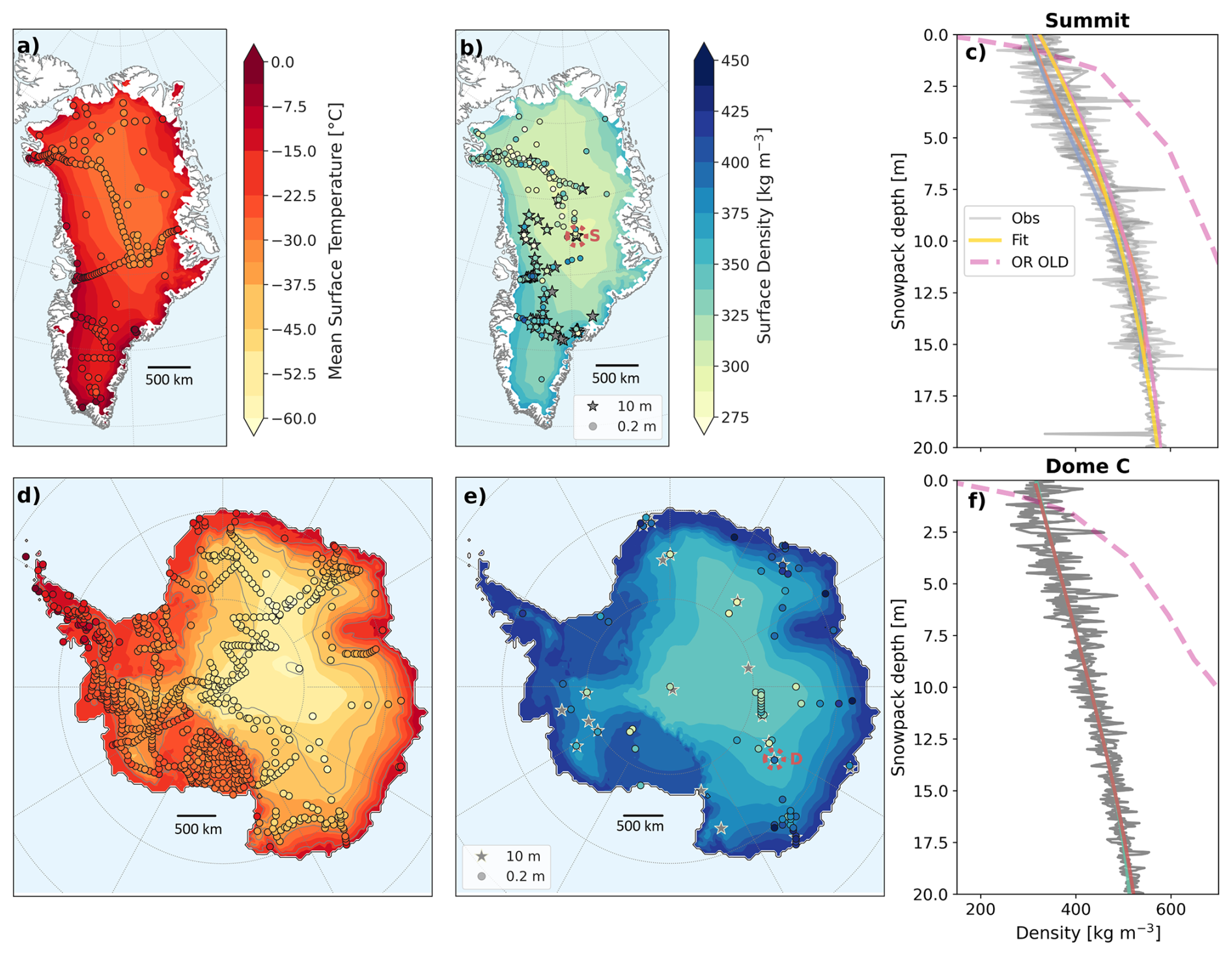
Figure 1 Mean annual surface temperature for Greenland (a) and Antarctica (d), observed at 10 m depth in the snowpack (circles). Color-filled areas are obtained with the initialization procedure (see Sect. 3.1). Mean surface density for Greenland (b) and Antarctica (e) for the observed top 20 cm (circles) and computed from the initialization procedure (color-filled areas). Star-shaped markers denote density profiles reaching 10 m depth. Red dashed circles indicate the location of the Summit station (“S”) in Greenland (b) and Dome C (“D”) in Antarctica (e). Observed density profiles at the Summit (c) and Dome C (f) station. Grey lines correspond to density observations and colored curves represent the fitted profiles obtained from the observed density profiles. The dashed pink curve shows the density profile computed by ORCHIDEE (OR OLD) with the standard version of the model (Sect. 2.3).

The second term of the right hand side of Eq. (2) represents the compaction by overburden pressure. It is driven by the vertical stress of the overlying snow, which induces sintering, reduces porosity, and leads to continuous deformation through mechanical creep. This process is the dominant contribution to dry snow densification. The snow viscosity η is expressed as a function of density and temperature:

$$\begin{array}{}\text{(4)}& \mathit{\eta }={\mathit{\eta }}_{\mathrm{0}}\cdot \exp \left[a_{\mathit{\eta }}\right(T_{\mathrm{f}}-T)+b_{\mathit{\eta }}\mathit{\rho }]\end{array}$$

where η₀ = 3.7 × 10⁷ $\mathrm{kg}{\mathrm{s}}^{-\mathrm{1}}{\mathrm{m}}^{-\mathrm{2}}$, a_η = 8.1 × 10⁻² K⁻¹ and b_η = 1.8 × 10⁻² m³ kg⁻¹. The values of the snow viscosity parameters provided by Anderson (1976) are not adapted to polar snow conditions, leading to excessive densification compared to observed density profiles (van Kampenhout et al., 2017) (Fig. 1c and f). In this study (Sect. 4), we calibrate these parameters to represent polar snow densification using the History Matching calibration method.

2.3 Experimental setup and forcing

We use the ORCHIDEE model in offline mode with a 30 min time step. The atmospheric forcing is provided by the polar-oriented regional atmospheric model MAR (Fettweis et al., 2017; Kittel et al., 2021), coupled to the SISVAT (Soil Ice Snow Vegetation Atmosphere Transfer) land surface scheme (Ridder and Schayes, 1997), that includes a multi-layered snow model based on the CROCUS model (Brun et al., 1989; Agosta et al., 2019). MAR has been extensively evaluated to represent surface mass balance, near-surface temperature and solid precipitation in comparison with in situ observations over Antarctica (Agosta et al., 2019) and with observations and model reconstructions over Greenland (Fettweis et al., 2017). Moreover, the intercomparison exercise GrSMBMIP higlights the good comparison of MAR with in situ SMB measurements over Greenland (Fettweis et al., 2020). MAR has also been shown to outperform the ERA5 reanalysis in representing the summer near-surface temperatures (Delhasse et al., 2020).

The ORCHIDEE model is forced every 3 h in terms of solid and liquid precipitation, surface pressure, wind speed at 10 m, temperature and specific humidity at 2 m, downward shortwave and longwave radiation. At each time step, the model uses incoming radiative fluxes in the short and longwave bands from MAR, and computes the upward shortwave and longwave radiation and the surface latent and sensible heat fluxes. These turbulent fluxes are obtained following the Monin–Obukhov turbulence theory (Monin and Obukhov, 2009) using the wind speed at 10 m, a drag coefficient and the atmosphere/surface gradient of temperature and specific humidity at 2 m (Charbit et al., 2024). The model also calculates the surface mass balance by accounting for solid and liquid precipitation from the forcings, as well as modeled sublimation and runoff over snow and ice.

We set up two configurations, one for GrIS and one for the AIS using the same stereographic grid as in the atmospheric forcing. For Greenland, we use MAR version 3.13 (Fettweis et al., 2023) with a horizontal resolution of 15 km, covering 1980–2019. For these offline ORCHIDEE experiments over GrIS, we rely on 2 sets of albedo parameters. We first use the assimilated albedo parameters from MODIS satellite albedo products (Raoult et al., 2023), referred hereafter to as ASIM12L. However, Charbit et al. (2024) showed that the ASIM12L albedo parameters led to a significant underestimation of runoff over GrIS. Therefore, we also use the albedo parameters set obtained from a manual tuning approach (Charbit et al., 2024) and designed to improve the agreement between the runoff simulated by MAR and ORCHIDEE. These albedo parameters will be referred to as OPT12L and are used only in Sect. 6.2. Since the MARv3.13 forcings were not available for Antarctica at the time this study was initiated, we use the MAR version 3.12, spanning 1980–2019 with a 35 km horizontal resolution (Davrinche et al., 2024). Both AIS and GrIS MAR simulations were forced every 6 h at their lateral boundaries by the ERA5 reanalysis (Hersbach et al., 2020). As albedo is more spatially uniform and temporally stable over the AIS than over the GrIS, we manually adjusted the albedo parameters in ORCHIDEE over the AIS, to better represent the surface conditions at Dome C. All AIS simulations use the same albedo parameters. The values for these three sets of albedo parameters can be found in Table S1 in the Supplement.

Pahaut (1976)Anderson (1976)Anderson (1976)

Table 1 Overview of the model configurations and developments included in each simulation. OR OLD corresponds to the original model configuration, OR OLD + INIT includes the snowpack initialization procedure, and OR NEW takes into account the different developments presented in this study.

Following this, to investigate the effect of the developments proposed in this study, we define three different ORCHIDEE configurations (Table 1). The reference simulation, presented as OR OLD, uses the same configuration introduced in Charbit et al. (2024). This experiment shows an underestimation of density at the surface and an excessive compaction at depth (Fig. 1c and f) and starts the simulation from a snow-free state over the ice sheet. The OR OLD + INIT configuration uses the new initialization procedure (Sect. 3.1), while OR NEW further includes updated model physics, with the new surface density parameterization (Sect. 3.2) and the calibrated viscosity parameters for polar regions (Sect. 4.3).

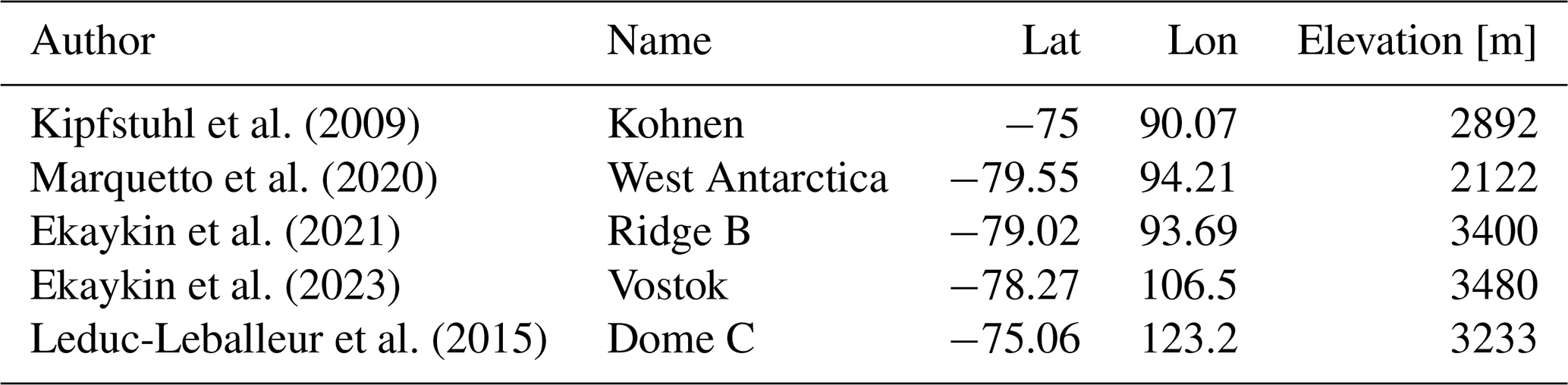
Kipfstuhl et al. (2009)Marquetto et al. (2020)Ekaykin et al. (2021)Ekaykin et al. (2023)Leduc-Leballeur et al. (2015)

Table 2 Additional density observations supplementing the SUMup database.

2.4 Observations

To improve the representation of snow densification, we use observations of snow temperature, accumulation and density in Greenland and Antarctica. From the SUMup collaborative database (Vandecrux et al., 2025), we use 3749 observations of snow temperature collected at different locations in Greenland, between 1930 and 2023, and 905 in various sites over Antarctica between 1957 to 2021 (Fig. 1a and d). The observations of snow accumulation are sourced, for Antarctica, from the GLACIOCLIM-SAMBA dataset, detailed in Favier et al. (2013) and updated by Wang et al. (2016), with 2981 observations over Antarctica, recorded between 1930 and 2009, and from the SUMup dataset for Greenland with 358 accumulation observations, collected between 1952 and 2023. Over Greenland and Antarctica, we only retain data for which the duration of observations is specified (ranging from a few days to several years). To investigate surface snow density, we use density profiles from the SUMup database and additional density sources listed in Table 2, containing measurements within the top 20 cm (560 observations in Greenland and 139 in Antarctica).

The representation of the vertical densification is assessed using 126 profiles extracted from the SUMup database (79 in Greenland and 49 in Antarctica) and two additional profiles located at Dome C in Antarctica (Leduc-Leballeur et al., 2015) (Fig. 1b and e). Among these observations, 102 reach depths of at least 10 m (79 in Greenland and 23 in Antarctica). For our study, we select two sites characterized by dry snow conditions: Summit (72.58° N, 38.50° W; 3254 $\mathrm{m}\mathrm{a}.\mathrm{s}.\mathrm{l}.$) and Dome C (75.06° S, 123.21° E; 3233 $\mathrm{m}\mathrm{a}.\mathrm{s}.\mathrm{l}.$). These locations present different climatic conditions. Dome C is characterized by an extremely cold and arid climate with mean annual surface temperatures of −55 °C (Buizert et al., 2021) and accumulation rates close to 30 $\mathrm{kg}{\mathrm{m}}^{-\mathrm{2}}{\mathrm{yr}}^{-\mathrm{1}}$ (28.6 $\mathrm{kg}{\mathrm{m}}^{-\mathrm{2}}{\mathrm{yr}}^{-\mathrm{1}}$ observed between 2006 and 2013;  Genthon et al., 2016). Summit exhibits a less cold environment, with a mean annual surface temperature observed of −31.4 °C observed between 1998 and 2017 (Vandecrux et al., 2020) and significantly higher accumulation rates of approximately 242 $\mathrm{kg}{\mathrm{m}}^{-\mathrm{2}}{\mathrm{yr}}^{-\mathrm{1}}$ recorded at Summit Camp between 2017 and 2020 (Howat, 2022). At Summit, five density profiles are selected, reaching at least 10 m depth, collected between 2006 and 2017 (Vandecrux et al., 2025). At Dome C, we use two density profiles collected in the 2012–2013 austral summer (Leduc-Leballeur et al., 2015). Figures 1c and f represent the observed density profiles at Summit and Dome C, respectively. To filter out density measurements fluctuations, we have applied a third-degree polynomial interpolation to the raw density profiles (Fig. 1c and f).

Table 3 Summary of observational data for model calibration and validation.

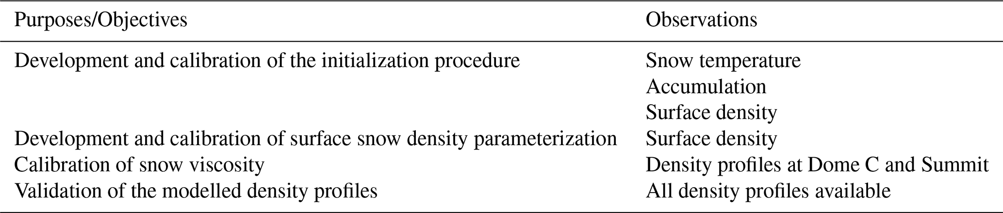
The observations described above are used for distinct purposes (see Table 3). The snow temperature, accumulation, and surface density observations are used to develop and calibrate the initialization procedure. The surface density observations are employed to design and calibrate the parameterization of surface snow densification. Finally for the snow compaction scheme, the vertical density profiles at Summit and Dome C are used for calibration, while the complete set of density profiles serves as an independent validation dataset.

To compare point observations and model gridded outputs, the observations are averaged on the ORCHIDEE stereographic grid (15 km resolution in Greenland, 35 km in Antarctica). After averaging temperature observations onto the model grid, we obtain 180 points in Greenland and 770 in Antarctica (Fig. 1a and d). We also compute the grid averaged accumulation, weighted by the corresponding duration of observations. This way, we obtain 76 grid-cell averages over Greenland, and 589 for Antarctica. For surface densities, we obtain 149 grid cell averages for Greenland and 79 for Antarctica (Fig. 1b and e).

3 New developments for polar snow in ORCHIDEE Explicit Snow

3.1 Snowpack initialization

ORCHIDEE was previously initialized without snow over ice sheet, relying on model accumulation through a 5-year spin-up period (Charbit et al., 2024). Here, we introduce a new method for initializing the snowpack over the Antarctic and Greenland ice sheets. This procedure enables the formation of a 10 m water equivalent (w$.\mathrm{e}.$) snowpack in low accumulation areas, such as the interior of AIS where several decades of simulation would be necessary to form a thick snowpack. Our initialization method expresses the initial density profile as a function of latitude and surface elevation only, making it easily adaptable to any snowpack model. It also initializes the surface temperature of the snowpack as well as the snowpack depth, which is considered uniform for Antarctica and variable for Greenland between the interior of the ice sheet and areas where net ablation is expected (see Appendix A4). Attention must be paid, as this initialization was developed using observations from recent decades, making it potentially not appropriate for very different climatic contexts from the present-day one. This method is presented in detail in Appendix A, and summarized hereafter. Here, we use the densification formulation proposed by Arthern et al. (2010) and further adapted by Ligtenberg et al. (2011):

$$\begin{array}{}\text{(5)}& \begin{array}{rl}{\displaystyle \frac{\mathrm{d}\mathit{\rho }}{\text{dz}}}=& C\cdot g\cdot \mathit{\gamma }\left(\ln \right(\stackrel{\mathrm{‾}}{A}\left)\right)\cdot \exp \left({\displaystyle \frac{E_{\mathrm{g}}-E_{\mathrm{c}}}{R\stackrel{\mathrm{‾}}{T_{\mathrm{s}}}}}\right)\cdot \mathit{\rho }\left(z\right)\\ & \times ({\mathit{\rho }}_{\text{ice}}-\mathit{\rho }(z\left)\right)\cdot \text{dz}\end{array}\end{array}$$

where $\stackrel{\mathrm{‾}}{A}$ is the local mean annual accumulation (in $\mathrm{kg}{\mathrm{m}}^{-\mathrm{2}}{\mathrm{yr}}^{-\mathrm{1}}$), $\stackrel{\mathrm{‾}}{T_{\mathrm{s}}}$ is the local mean annual surface temperature (in K), g the gravitational acceleration (9.81 m s⁻²), ρ_ice the ice density (917 kg m⁻³), dz the snow layer thickness (in m), R the gas constant (8.31 $\mathrm{J}{\mathrm{K}}^{-\mathrm{1}}{\mathrm{mol}}^{-\mathrm{1}}$), E_g and E_c the activation energies of grain growth (4.24 × 10⁴ J mol⁻¹) and compaction (6 × 10⁴ J mol⁻¹), respectively. C is an unitless constant with different values above (0.03) and below (0.07) the critical density ρ = 550 kg m⁻³, reflecting a faster densification rate near the surface.

The γ factor represents a correction to the accumulation term introduced by Ligtenberg et al. (2011). Their study revealed that the ratio of modeled to observed depths at which snow reaches critical densities of 550 and 830 kg m⁻³ is strongly correlated with mean annual accumulation across Antarctica. To account for this dependency, we use the same corrective term except that we applied a scaling factor of 0.9 for densities greater than 550 kg m⁻³ to better match the observed density profile at a depth corresponding to 830 kg m⁻³ in Antarctica:

$$\begin{array}{}\text{(6)}& \mathit{\gamma }(x,y)=\left\{\begin{array}{l}\begin{array}{c}max(\mathrm{1.435}-\mathrm{0.151}\cdot \ln (\stackrel{\mathrm{‾}}{A}(x,y)),\\ {\mathit{\gamma }}_{min})\text{ for }\mathit{\rho }\le \mathrm{550}\mathrm{kg}{\mathrm{m}}^{-\mathrm{3}}\end{array}\\ \begin{array}{c}max(\mathrm{0.9}\cdot [\mathrm{2.366}-\mathrm{0.293}\cdot \ln \left(\stackrel{\mathrm{‾}}{A}\right(x,y\left)\right)],\\ {\mathit{\gamma }}_{min})\text{ for }\mathit{\rho }>\mathrm{550}\mathrm{kg}{\mathrm{m}}^{-\mathrm{3}}\end{array}\end{array}\right.\end{array}$$

where γ_min is the minimal correction equal to 0.25 as in Ligtenberg et al. (2011). This γ term is generally calibrated to account for surface climate biases (Brils et al., 2022; Veldhuijsen et al., 2023).

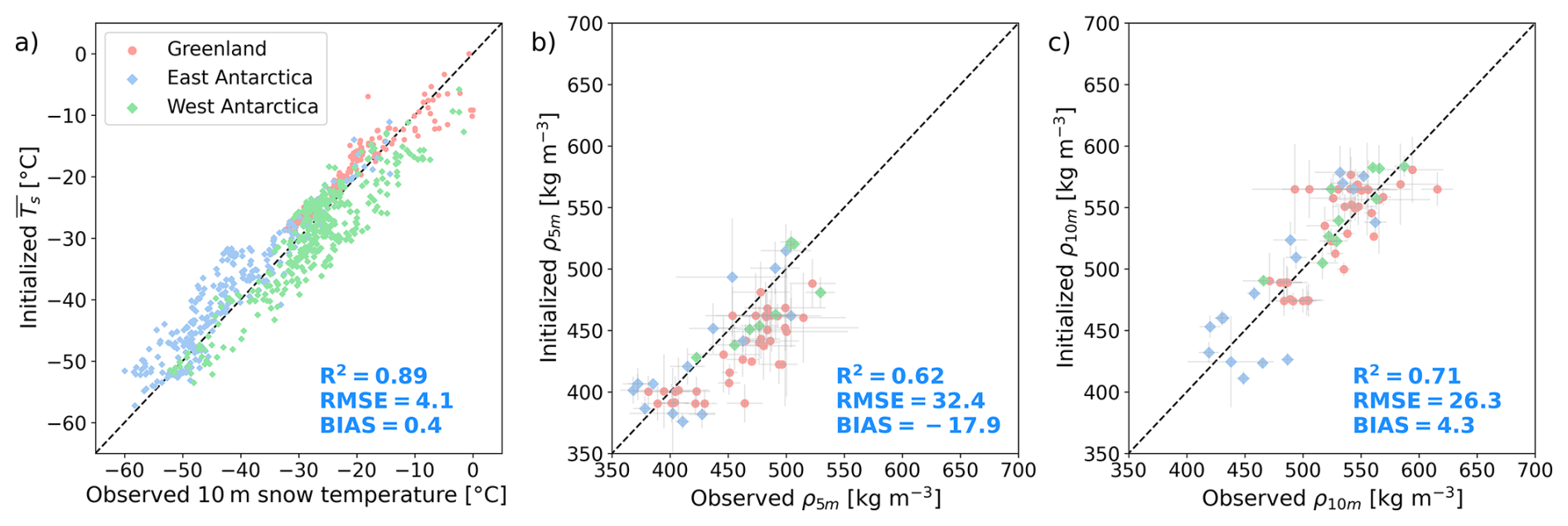
Figure 2 (a) Mean surface temperature $\stackrel{\mathrm{‾}}{T_{\mathrm{s}}}$ obtained from the initialization procedure represented as a function of the observed 10 m snow temperature. (b, c) Initialized snow density at 5 m (b) and 10 m (c) depth versus observed densities at 5 m (b) and 10 m (c) across Greenland, East Antarctica, and West Antarctica. Statistical indicators (correlation coefficient R², RMSE, and bias) are reported in blue. Locations in Greenland, East Antarctica, and West Antarctica are marked in red, cyan, and green, respectively. Error bars represent observational uncertainties (see Supplement).

After integration of Eq. (5) (Appendix A), the explicit formulation of the density profile is expressed as a function of the mean surface temperature $\stackrel{\mathrm{‾}}{T_{\mathrm{s}}}$, the logarithm of the mean annual accumulation rate $\ln \left(\stackrel{\mathrm{‾}}{A}\right)$, and the surface density ρ_s. We estimate these key variables as a function of surface elevation and latitude, based on physical considerations and empirical relationships derived from observations and modeling outputs, and detailed in Appendix A. This method provides a final parameterization of the density profile that depends only on latitude and elevation. Other studies have used densification equations to initialize snow models, such as CRYOWRF, which relies on the Firn Densification Model to calculate the initial density profile (Gerber et al., 2023). The strength of our method is its independence from additional models, enabling standalone initialisation for any snowpack model. Over Greenland, the parameterizations yield root mean square errors (RMSE) representing 11 % of the mean accumulation logarithm (RMSE = 0.60 ln ($\mathrm{kg}{\mathrm{m}}^{-\mathrm{2}}{\mathrm{yr}}^{-\mathrm{1}}$)) and 11 % of the mean surface density (36.4 kg m⁻³). For the surface temperature, the RMSE is equal to 3.1 °C in Greenland (compared to an observed mean temperature of −20.6 °C), while over Antarctica, the RMSE reaches 4.6 °C (compared to an observed mean temperature of −32.8 °C). The corresponding errors over the AIS represent 12.2 % of the mean accumulation logarithm (0.56 ln ($\mathrm{kg}{\mathrm{m}}^{-\mathrm{2}}{\mathrm{yr}}^{-\mathrm{1}}$)) and 8 % of the mean surface density (29.4 kg m⁻³). When evaluated over both ice sheets, the parameterized surface mean temperature correlates strongly with the observed 10 m snow temperature, with a difference of only 0.4 °C and a correlation coefficient of 0.89. (Fig. 2a). This initialization method can generate a polar snowpack of prescribed depth over the AIS and GrIS. As ablation is negligible in Antarctica, we consider a spatially uniform snowpack thickness set to 10 m. Conversely, in Greenland, the snow depth varies spatially from the edges to the interior of the ice sheet where it is also fixed at 10 m (see Appendix A4). The estimated mean annual surface temperature of the snowpack is also used to initialize snow and ice temperatures of all snow and ice layers at the beginning of the simulation.

The initialized snowpack density is compared to observations under dry snow conditions, in order to isolate the densification driven by the snow compaction (Fig. 2b and c). In ablation zones, where melt is significant, additional densification occurs from the refreezing of meltwater retained within the snowpack. This process is not accounted for in the initialization procedure. Overall, the initialized snowpack density agrees well with observations under dry snow conditions. The RMSE represents 7 % of the mean snow density at 5 m depth (RMSE = 32.4 kg m⁻³). At 10 m depth, the comparison with observations performs even better, with reduced RMSE (26.3 kg m⁻³, 5.1 % of the mean snow density at this depth) and bias (4.3 kg m⁻³; 0.9 %).

3.2 Surface snow density

Over Greenland and Antarctica, surface snow densities measured in the uppermost centimeters of the snowpack are significantly higher than the range of the Pahaut (1976)'s formulation, ranging from 200 to 400 kg m⁻³ (Fausto et al., 2018; Agosta et al., 2019). In this way, applied to GrIS and AIS this formulation leads to a significant underestimation of surface snow density when compared to observations (Sect. 5.1).

To represent high surface densities in polar regions, we choose to compensate the limited physical understanding of the processes involved, by introducing a new surface density parameterization, common to both ice sheets and based only on wind speed. In the following, surface snow density will be considered as the mean density of the upper 20 cm of the snowpack. The new parameterization is applied to the modeled fresh snow density in ORCHIDEE, i.e. only at time steps when snowfall occurs, in order to determine the deposited snow density. Similar approaches have been employed in Arctic (Barrere et al., 2017) and Antarctic studies (Amory et al., 2021; Lenaerts et al., 2012; Keenan et al., 2021; Veldhuijsen et al., 2023). Moreover, using both Greenland and Antarctic surface snow observations, we find that the observed surface density correlates more strongly with wind speed than with air temperature, supporting our choice to use a wind parameterization for surface density (Fig. A3).

If surface density is expressed as a linear function of instantaneous wind speed, then the temporal average of surface density can be related to wind speed weighted by precipitation. In order to calibrate the formulation, we compare gridded-averaged surface snow density observations from Greenland and Antarctica with the precipitation weighted 10 m wind speed climatological average (1980–2019) simulated by MAR (Fig.3).

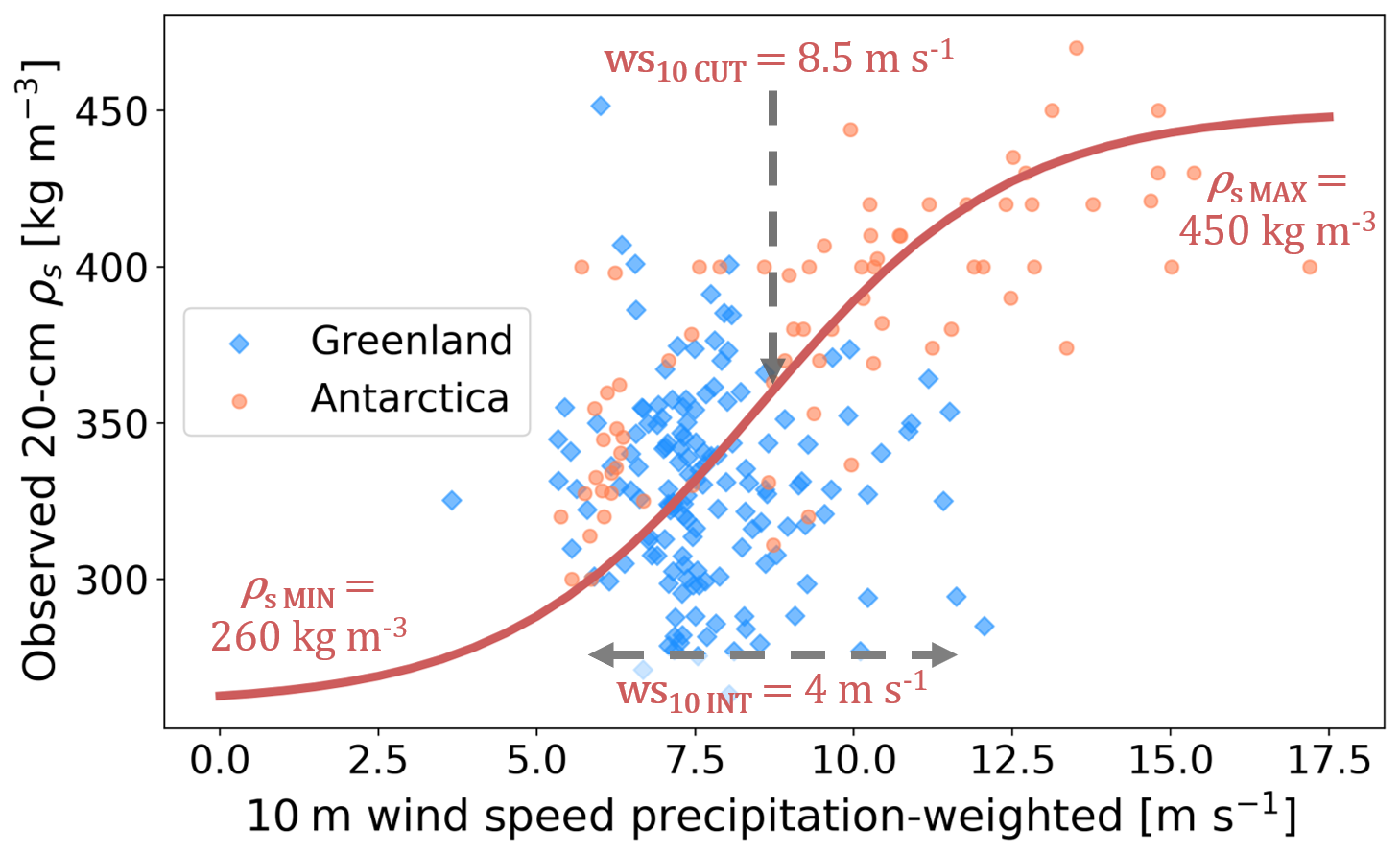
Figure 3 Observed mean surface snow densities in the upper 20 cm of the snowpack represented as a function of the climatological average (1980–2019) of the 10 m wind speed simulated by MAR and weighted by the amount of snowfall during the same period. Observations are presented in blue for Greenland and orange for Antarctica. The red line represents the wind speed parameterization of surface snow density presented in this study.

In Antarctica, a linear relationship appears between wind speed and surface snow density. In contrast, Greenland shows a more heterogeneous pattern, with observations clustering around 320 kg m⁻³, in agreement with Fausto et al. (2018). Here, we propose a new expression for surface snow density ρ_s, defined as a function of the wind speed at 10 m,

$$\begin{array}{}\text{(7)}& \begin{array}{rl}{\mathit{\rho }}_{\mathrm{s}}\left({\text{ws}}_{\mathrm{10}}\right)=& {\mathit{\rho }}_{\mathrm{s}\text{MIN}}+({\mathit{\rho }}_{\mathrm{s}\text{MAX}}-{\mathit{\rho }}_{\mathrm{s}\text{MIN}})\\ & \times \left(\mathrm{1}+\text{tanh}\left({\displaystyle \frac{{\text{ws}}_{\mathrm{10}}-{\text{ws}}_{\mathrm{10}\text{CUT}}}{{\text{ws}}_{\mathrm{10}\text{INT}}}}\right)\right)/\mathrm{2}\end{array}\end{array}$$

with ρ_s MIN = 260 kg m⁻³ the minimum surface snow density reached at low wind speeds (< 5 m s⁻¹), ρ_s MAX = 450 kg m⁻³ the maximum surface snow density reached at high wind speeds (> 15 m s⁻¹), ws_10 CUT = 8.5 m s⁻¹ the wind speed at the inflection point of the hyperbolic tangent, ws_s INT = 4.0 m s⁻¹ the width of the interval over which the hyperbolic transition from minimum to maximum density takes place. For Greenland, we imposed a maximum density of 400 kg m⁻³ to ensure a realistic range of surface densities in this region, as observations generally do not exceed this value (Fausto et al., 2018). For Antarctica, the maximum density remains equal to ρ_s  MAX.

Applied to both ice sheets, the formulation yields a RMSE of 40.3 kg m⁻³ (11.3 % compared to the averaged surface density) and a bias of 1.9 kg m⁻³ (i.e. 0.5 %), indicating a satisfactory agreement with observations. Although the parameterization does not fully capture the observed spatial heterogeneity of surface snow density, particularly over Greenland, it nevertheless reproduces the observed mean surface density and thereby corrects the strong negative bias resulting from Eq. (1).

4 History Matching calibration method

4.1 History Matching theory

History Matching (HM) is a method for calibrating parameters (Couvreux et al., 2021; Hourdin et al., 2021), implemented within the ORCHIDEE Data Assimilation Systems (ORCHIDAS MacBean et al., 2022; Raoult et al., 2024). This procedure is based on Gaussian process emulation and is designed to constrain the free parameters of complex models. It has been applied to calibrate atmospheric, ocean and Earth system models (Couvreux et al., 2021; Hourdin et al., 2021; Villefranque et al., 2021; Williamson et al., 2017; Hourdin et al., 2023), as well as ice sheet models (McNeall et al., 2013) and land surface models (Baker et al., 2022; McNeall et al., 2024). Originally developed to calibrate model parameters at the process level, HM operates in ORCHIDAS using offline ORCHIDEE simulations in a single-column model framework. This approach has previously been applied to the ORCHIDEE model to simulate net ecosystem exchange and latent heat fluxes (Raoult et al., 2024). This calibration approach differs from the traditional data assimilation method, which primarily focuses on identifying the optimal parameters that best match observations by minimizing a cost function. In contrast, HM aims to identify regions of the parameter space that are “not plausible” given the constraints predefined through observations, i.e. leading to model outputs inconsistent with observations.

The calibration starts by sampling the prior parameter space using a Latin Hypercube design (Morris and Mitchell, 1995), to efficiently explore the space and maximize the information gained from each parameter combination. Following the recommendation of Loeppky et al. (2009), we use a sample size equal to $N=\mathrm{10}\cdot P$, where P is the number of parameters being calibrated. One-dimensional ORCHIDEE simulations are performed for each sampled set of parameters. Iteratively, Gaussian process emulators are then constructed to capture the relationship between model parameters and scalar metrics, specifically designed to characterize the physical processes under study. The construction of the Gaussian process emulators is done following the methodology presented in Williamson et al. (2013) and the R-scripts from Couvreux et al. (2021). Each metric is associated with its own emulator, which is then used to predict metric values across the full parameter space. This enables the identification of parameter regions that are inconsistent with observations using an implausibility criterion I, used to reduce the parameter space. The implausibility is defined as follows:

$$\begin{array}{}\text{(8)}& I\left(x\right)={\displaystyle \frac{|m-E[G\left(x\right)\left]\right|}{\sqrt{{\mathit{\sigma }}_{\text{obs}}^{\mathrm{2}}+{\mathit{\sigma }}_{\text{OR}}^{\mathrm{2}}+\text{Var}\left[G\right(x\left)\right]}}}\end{array}$$

with x being a sample of the parameter space, m the reference observed metric, E[G(x)] the value predicted by the emulator G(x). The implausibility accounts for the aggregated uncertainty, computed as the square root of the sum of squared contributions from three sources: the observational (σ_obs), model (σ_OR), and emulator (Var[G(x)]) uncertainties.

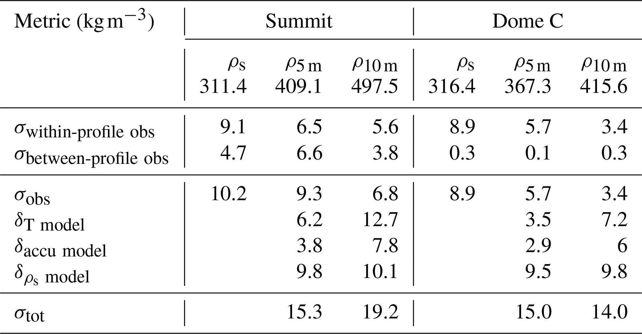
Table 4 Observed metrics and associated uncertainties for surface density (ρ_s), densities at 5 m (ρ_5 m) and 10 m (ρ_10 m) for Summit and Dome C. Observational (σ_obs) and model uncertainties (δ_T  model, δ_{accu  model}, ${\mathit{\delta }}_{{\mathit{\rho }}_{\mathrm{s}}\text{model}}$) are reported, as well as the total uncertainties (σ_tot).

This criterion is computed independently for each metric, and used to define the subregion of the parameter space that is not inconsistent with the reference observational metrics, also called the NROY space for “Not Ruled Out Yet”. The NROY space corresponds to the region of the parameter space where the implausiblity is smaller than a defined threshold. For the first iterations (waves) of the algorithm, it is common to set the implausibility cut-off to 3, following the 3σ rule stating that 99.7 % of the probability density for any unimodal distribution is comprised within 3 standard deviations of the mean. As the NROY space is progressively reduced during successive waves, this threshold is lowered to 2 for the final wave. With the progressive reduction in emulator uncertainty, decreasing the implausibility cut-off is a standard step in the calibration procedure (Williamson et al., 2017; Hourdin et al., 2021).

4.2 Metrics for densification and uncertainty quantification

In this study, we use the HM method, described in Sect. 4.1, to calibrate three parameters of the snow viscosity defined by Anderson (1976): η₀, a_η and b_η. We calibrate ORCHIDEE using 1D simulations over two dry snow locations, one in Greenland (Summit, 5 density profiles) and one in Antarctica (Dome C, 2 density profiles), presented in Sect. 2.4 (Fig. 1c and f). For each density profile, we apply a third degree polynomial interpolation (called “fit” herefafter) to smooth the observations. In this way, in the 1D simulations, the surface snow density (ρ_s) is prescribed using the average of the fitted surface snow density (Table 4). In addition, to characterize the dry snow densification profiles, we define two metrics for each location: density at 5 m (ρ_5 m) and at 10 m (ρ_10 m). Each metric is obtained from the fit of the observed density profiles, and is associated with an uncertainty estimate that accounts for both observational and model-related uncertainty.

Observational uncertainties are estimated by combining two sources of uncertainty. We distinguish within-profile uncertainty, which captures the vertical variability for a given profile around the considered depth, and between-profiles uncertainty, which reflects variability across different profiles at the same site, related to either spatial or temporal variability. Here, we present the observational uncertainties for the metrics (ρ_5 m and ρ_10 m) and the observed surface density (ρ_s). First, within-profile variability is quantified as the Root Mean Square (RMS) of the mean deviation (taken as $\frac{\mathit{\sigma }}{\sqrt{n}}$) across a vertical window around the target depth (4 to 6 m for ρ_5 m, 9 to 11 m for ρ_10 m, 0 to 1 m for ρ_s), e.g. for ρ_5 m:

$$\begin{array}{}\text{(9)}& {\mathit{\sigma }}_{\text{within-profile}\mathrm{5}\mathrm{m}}=\sqrt{{\displaystyle \frac{\mathrm{1}}{l}}\sum _{i=\mathrm{1}}^l{\left({\displaystyle \frac{\mathit{\sigma }\left({\mathit{\rho }}_{\text{obs}i\mathrm{4}\mathrm{m}<z<\mathrm{6}\mathrm{m}}\right)}{\sqrt{n_i}}}\right)}^{\mathrm{2}}}\end{array}$$

where l is the number of observed density profiles available, n_i the number of observations of a given profile i within the vertical window around the target depth, ρ_smoothed i and ρ_obs i the observed density of the given profile i within the same vertical window.

Second, between-profiles variability is estimated as the standard deviation of the density metrics across all profiles for each location, divided by the square root of the number of profiles, e.g. for ρ_5 m:

$$\begin{array}{}\text{(10)}& {\mathit{\sigma }}_{\text{between-profiles}\mathrm{5}\mathrm{m}}={\displaystyle \frac{\mathit{\sigma }\left({\mathit{\rho }}_{\text{smoothed}\mathrm{5}\mathrm{m}\mathrm{1},\mathrm{\dots },l}\right)}{\sqrt{l}}}\end{array}$$

where ${\mathit{\rho }}_{\text{smoothed}\mathrm{5}\mathrm{m}\mathrm{1},\mathrm{\dots },l}$ is the vector of the l density metrics (here ρ_5 m) resulting from the polynomial interpolation of the corresponding observed density profile.

These two components (σ_{within-profile} and σ_{between-profiles}) are then combined using the root sum square to consider independently both uncertainties, yielding the observational uncertainty for each metric (σ_obs 5 m, σ_obs 10 m) and for surface density (${\mathit{\sigma }}_{{\mathit{\rho }}_{\mathrm{s}}\text{obs}}$). In this way, at 5 m, mean densities from fitted profiles are equal to 409.1 and 367.3 kg m⁻³ at Summit and Dome C, associated with observational uncertainties equal to ± 9.3 and ± 5.7 kg m⁻³. At 10 m, we obtain, respectively 497.5 and 415.6 kg m⁻³, with observational uncertainties of ± 6.8 and ± 3.4 kg m⁻³. The observed surface densities are equal to 311.4 ± 10.2 kg m⁻³ at Summit and 316.4 ± 9.2 kg m⁻³ at Dome C (Table 4).

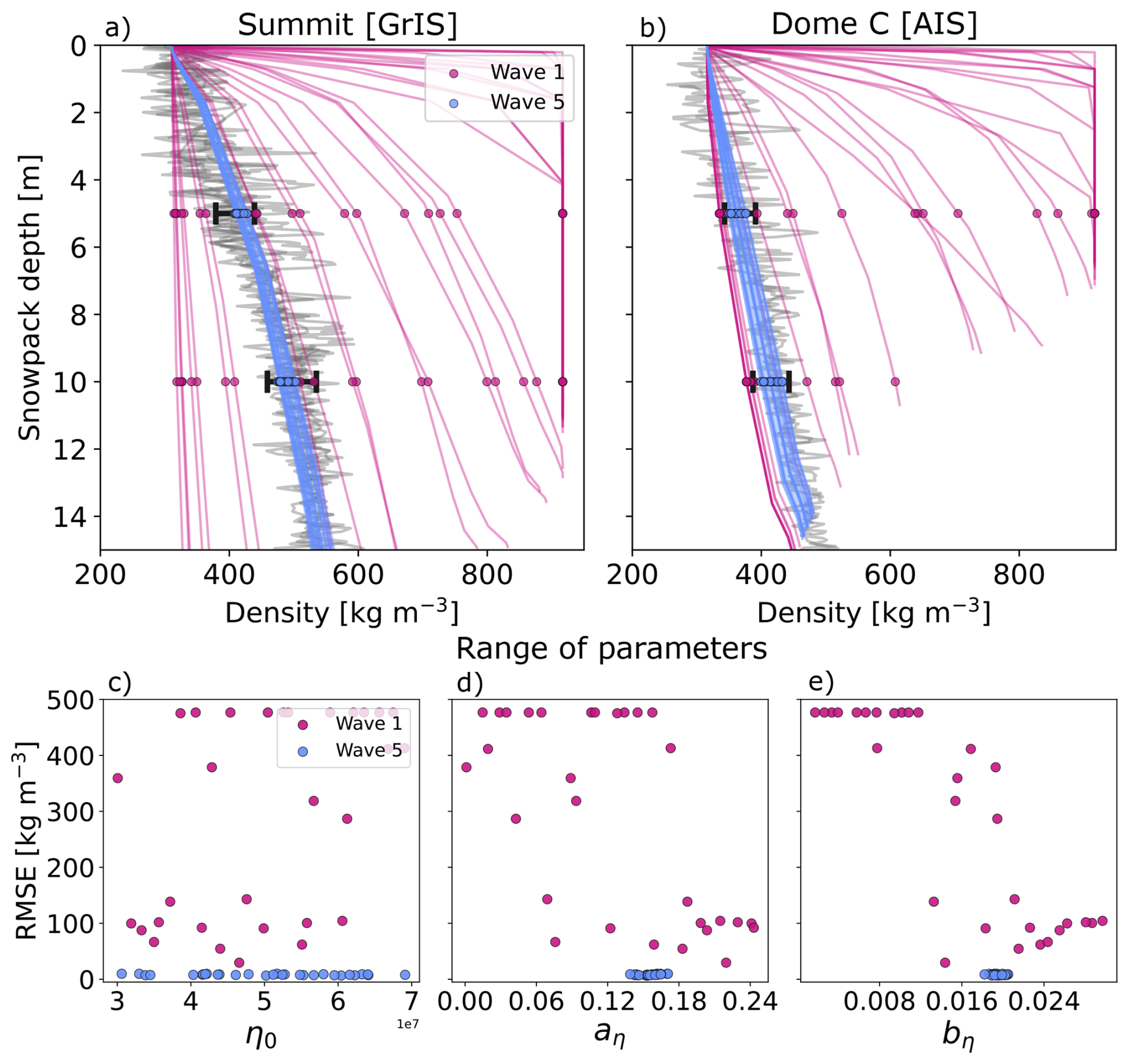
Figure 4 (a, b) Evolution of density profiles simulated by ORCHIDEE in 2019, after 40 years of simulation for Summit (a) and Dome C (b) along the first and fifth waves of the HM method. Waves 1 and 5 are, respectively represented in pink and blue. (c–e) Density metrics at 5 and 10 m are shown with dots. Reduction of the parameter ranges of η₀ (c), a_η (d) and b_η (e) between the first and the fifth wave, compared to the RMSE accounting for the metrics ρ_5 m and ρ_10 m at each location.

In addition to the observational uncertainty, we need to account for modeling uncertainties. We evaluate the sensitivity of the metrics ρ_5 m and ρ_10 m to biases in the modeled snow temperature, accumulation and surface snow density using the steady-state formulation of Ligtenberg et al. (2011) (Eq. 5, Sect. 3.1). These biases are evaluated by considering the 40 years integrated accumulation and the final year of snow temperature simulated by ORCHIDEE in comparison with the in situ observations presented in Sect. 2.4. We obtain temperature biases of +2.0 °C at Dome C and +2.6 °C at Summit, and accumulation biases of 12.4 $\mathrm{kg}{\mathrm{m}}^{-\mathrm{2}}{\mathrm{yr}}^{-\mathrm{1}}$ at Dome C and −54 $\mathrm{kg}{\mathrm{m}}^{-\mathrm{2}}{\mathrm{yr}}^{-\mathrm{1}}$ at Summit. We compute new steady state density profiles after adding the absolute value of these biases to the observed temperature and accumulation, using both positive and negative perturbations. The difference between the two perturbed steady state profiles is assumed to represent the model sensitivity to temperature and accumulation biases. The uncertainty is then estimated for ρ_5 m and ρ_10 m, as half this difference (δ_{accu  model} and δ_T  model). The same method is applied for ρ_s by injecting observed surface snow density uncertainty ${\mathit{\sigma }}_{\text{obs}{\mathit{\rho }}_{\mathrm{s}}}$, defined previously, in the steady state densification equation for each location separately.

Then, the final model uncertainty for each metric is obtained by Root Sum Square aggregation of the uncertainties presented previously, e.g. for ρ_5 m:

$$\begin{array}{}\text{(11)}& {\mathit{\sigma }}_{{\mathit{\rho }}_{\mathrm{5}\mathrm{m}}}=\sqrt{\begin{array}{c}{\mathit{\sigma }}_{\text{obs}{\mathit{\rho }}_{\mathrm{5}\mathrm{m}}}^{\mathrm{2}}+{\mathit{\delta }}_{\text{accu\hspace{0.17em}\hspace{0.17em}model}\mathrm{5}\mathrm{m}}^{\mathrm{2}}+{\mathit{\delta }}_{T\text{model}\mathrm{5}\mathrm{m}}^{\mathrm{2}}\\ +{\mathit{\delta }}_{{\mathit{\rho }}_{\mathrm{s}}\text{model}\mathrm{5}\mathrm{m}}^{\mathrm{2}}\end{array}}\end{array}$$

This yields total uncertainties of ± 15.3 and ± 19.2 kg m⁻³ for ρ_5 m and ρ_10 m at Summit, and ± 15.0 and ± 14.0 kg m⁻³, respectively, at Dome C (Table 4).

4.3 Snow viscosity calibration with 1D simulations

The HM method is applied to calibrate the viscosity parameters of Eqs. (2) and (4), with the objective of identifying parameter sets consistent with snow densification at both Summit and Dome C. Since we calibrate three viscosity parameters, the sample size is equal to 3×10 sets of parameters, sampled at each wave of the HM algorithm, following Loeppky et al. (2009) (see also Sect. 4.1). For each parameter set and each location, we run 1D ORCHIDEE simulations (1 at Summit and 1 at Dome C) and compute the corresponding metrics. It results in 60 simulated ρ_5 m and ρ_10 m values for each wave (3 parameters × 10 simulations × 2 locations), used to construct the Gaussian process emulators. In total, we perform 5 waves, to progressively reduce the parameter space and obtain parameter values providing consistent densification metrics ρ_5 m and ρ_10 m.

Table 5 Free parameters of the Anderson (1976) viscosity equation used in the calibration. “Anderson value” corresponds to the default value of each parameter, “Prior range” to the initial parameter bounds, and “Calibrated range” and “Calibration result” to the ranges and values retained after the HM method.

During the first wave, the simulated densities at 5 and 10 m depths exhibit a wide spread, ranging from 300 to 900 kg m⁻³, highlighting the strong sensitivity of modeled densification to the viscosity parameters (Fig. 4a and b). After five waves, the parameter space is reduced by 99.6 %, and the resulting viscosity parameters are able to capture observed densification rates. At wave 5, the simulated ρ_5 m and ρ_10 m remain within the bounds of the metrics uncertainties at both Summit and Dome C.

The HM method also leads to a substantial reduction of the viscosity parameter ranges between the first and fifth wave (Fig. 4c and e; Table 5). The sensitivity of snow viscosity to temperature, governed by a_η, is increased from 0.081 to values converging between 0.138 and 0.17 K⁻¹, highlighting the stronger control of temperature on polar densification compared to the former formulation. This suggests that snow viscosity was underestimated in the original parameterization (Anderson, 1976), due to an insufficient influence of the temperature. In contrast, the sensitivity of the viscosity to density, controlled by parameter b_η, remains close to the values proposed by Anderson (1976), with a final range between 0.018 and 0.02 ${\mathrm{m}}^{-\mathrm{3}}{\mathrm{kg}}^{-\mathrm{1}}$ (0.018 ${\mathrm{m}}^{-\mathrm{3}}{\mathrm{kg}}^{-\mathrm{1}}$initially). By comparison, the parameter η₀, which sets the reference viscosity, exhibits limited influence on the metrics, as its variability does not significantly affect model performance within the explored range. This suggests that either the selected metrics are not sensitive enough to constrain η₀ or that polar snow densification is primarily driven by the temperature and density sensitivities (a_η and b_η), with η₀ playing only a minor role. Equifinality may also occur, with the calibrated sensitivity to temperature and density compensating for variations in the reference viscosity. The analysis of the final parameter space reveals a strong correlation between a_η and b_η (Fig. A4). These parameter refinements are reflected in the reduction of the aggregated RMSE, i.e. the RMSE computed combining the four density metrics (at 5 and 10 m depths over Summit and Dome C):

$$\begin{array}{}\text{(12)}& \sqrt{{\displaystyle \frac{\mathrm{1}}{n}}\sum _{i=\mathrm{0}}^n\left[\right({\mathit{\rho }}_{i\mathrm{5}\mathrm{m}}-{\mathit{\rho }}_{i\mathrm{5}\mathrm{m}\text{obs}}{)}^{\mathrm{2}}+({\mathit{\rho }}_{i\mathrm{10}\mathrm{m}}-{\mathit{\rho }}_{i\mathrm{10}\mathrm{m}\text{obs}}{)}^{\mathrm{2}}]}\end{array}$$

where n is the number of locations studied (Summit and Dome C). The aggregated RMSE decreases substantially from an initial range of 50 to 500 kg m⁻³ to a reduced range between 6.85 and 9.87 kg m⁻³ after five calibration waves (Fig. 4c–e). We select the parameter set that minimizes the aggregated RMSE (6.85 kg m⁻³) across both locations (Table 5).

5 Application to the Greenland and Antarctic ice sheets

The developments presented in the previous sections have led to noticeable improvements in the simulated density profiles for Summit and Dome C compared to available observations. In this section, we now perform offline ORCHIDEE simulations (1980–2019) for the entire GrIS and AIS to estimate their response to these new developments.

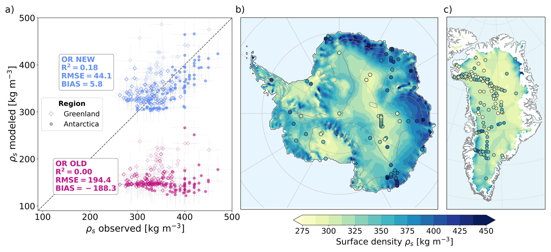
Figure 5 (a) Comparison of 40 years averaged (1980–2019) modeled surface snow density (computed as the average density of the top 20 cm of the snowpack) with observed surface snow density from Greenland (open diamond) and Antarctica (solid circle). Model results are shown for the previous ORCHIDEE formulation (OR OLD,purple; Pahaut, 1976) and the new formulation (OR NEW, blue). Error bars represent observational uncertainties (see Supplement). (b, c) Spatial comparison of 40 years averaged modeled surface snow density with observations (in dots) in Antarctica (b) and Greenland (c).

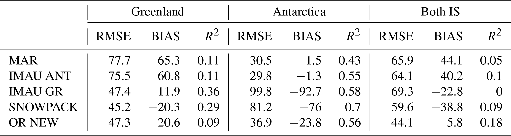
Table 6 Surface snow density statistical indicators for MAR, IMAU and ORCHIDEE surface snow formulations.

5.1 Surface snow density

We compare the new formulation of the surface snow density computed by ORCHIDEE with observations of surface snow densities (Fig. 5). This comparison is made for the former formulation (Pahaut, 1976) and the new one proposed in this study (Eq. 7). Surface snow densities are computed as the average density of the top 20 cm of the snowpack over a 40 years period (1980–2019). As previously mentioned, the Pahaut (1976) parameterization strongly underestimates surface snow density for both AIS and GrIS, with a negative bias of −188.3 kg m⁻³, representing 53 % of the average observed ρ_s. The new formulation shows an overall good representation of surface density with a bias of only 5.8 kg m⁻³. Regional analysis reveals a positive bias over Greenland (20.6 kg m⁻³, i.e. 6.2 % with reference to the observed average ρ_s) and a negative bias over Antarctica (−23.8 kg m⁻³, 6.3 %). However, surface snow densities can be affected by melt-refreeze processes, particularly over Greenland. These processes increase snow density through the accumulation of refrozen meltwater. Furthermore, this additional densification is represented within the snow scheme, but is not explicitly included in the surface snow density parameterization. This can constitute a potential bias for our evaluation.

We account for this effect by excluding simulated surface snow densities where the 40 years average refreezing rate in the top 20 cm of the snowpack exceeds 0.1 $\mathrm{kg}{\mathrm{m}}^{-\mathrm{2}}{\mathrm{d}}^{-\mathrm{1}}$. These locations are represented by transparent dots in Fig. 5a.

Excluding the Greenland locations affected by refreeze processes improves the computed surface density, when considering both ice sheets, with a negative bias of −3.5 kg m⁻³ and a reduced RMSE equal to 34.8 kg m⁻³ (1 % and 9.8 % compared to the observed averaged surface snow density, respectively). This highlights the need for future studies to investigate the ORCHIDEE representation of refrozen areas in Greenland. Moreover, the new parameterization generally reproduces the large-scale spatial gradients in surface snow density over both ice sheets (Fig. 5b and c). It captures the higher densities along the wind exposed coastal margins, especially over Antarctica.

In addition, we conduct an inter-model comparison by implementing in ORCHIDEE the surface snow parameterizations from MAR over Antarctica (Kittel et al., 2021), from the IMAU-Firn densification model over both ice sheets (IMAU-FDM; Lenaerts et al., 2012; Veldhuijsen et al., 2023; Brils et al., 2022) and SNOWPACK over Antarctica (Groot Zwaaftink et al., 2013) (see Eqs. S9–S12 in the Supplement). Both MAR and SNOWPACK formulations of surface snow density are based only on 10 m wind speed and were developed for Antarctica. The IMAU-FDM formulation calibrated for Antarctic conditions relies on the 10 m wind speed and near surface temperature (T_2 m), while the one developed for Greenland depends only of the near surface temperature.

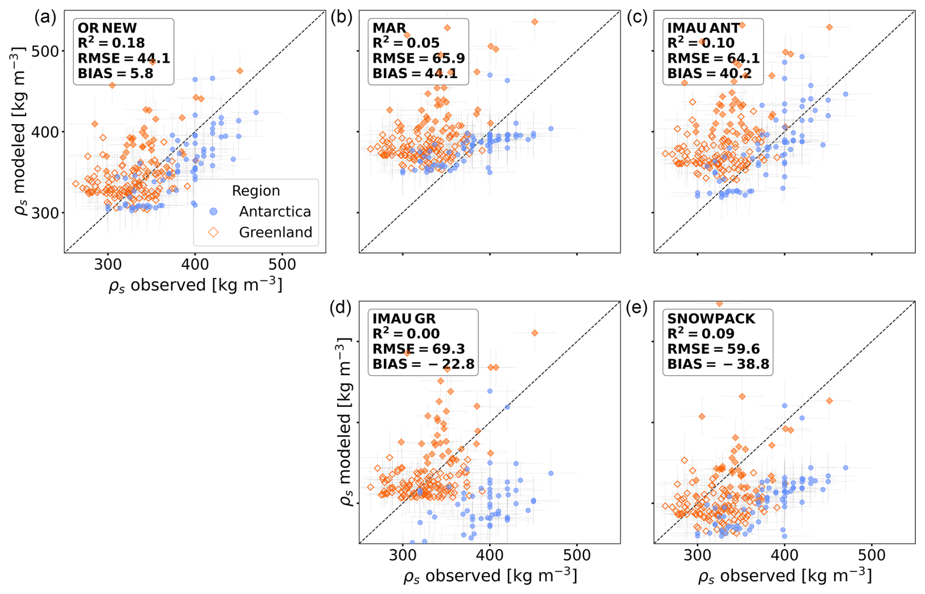
Figure 6 40 years average surface snow density compared to observations, modeled by (a) the new wind parameterization in ORCHIDEE, (b) the wind parameterization developed for Antarctica in MAR (Kittel et al., 2021), (c) the wind and temperature parameterization developped for Antarctica in IMAU (Lenaerts et al., 2012; Veldhuijsen et al., 2023), (d) temperature parameterization developped for Greenland in IMAU (Ligtenberg et al., 2018) and (e) the wind paramerization developped in SNOWPACK (Groot Zwaaftink et al., 2013). Locations are specified with orange open diamond and blue solid circle for Greenland and Antarctica, respectively. Shaded points are locations where the 40 years averaged refreeze in the top 20 cm of the snowpack is larger than 0.1 mm d⁻¹. Error bars represent observational uncertainties (see Supplement).

We test these formulations with offline ORCHIDEE simulations over Greenland and Antarctica for the 1980–2019 period. Model outputs are evaluated considering the top 20 cm for surface snow densities (Fig. 6). Both the IMAU-FDM over Antarctica (IMAU ANT) and MAR parameterizations perform well over Antarctica, with biases of only −1.3 and 1.5 kg m⁻³, respectively, representing differences of only 0.3 % and 0.4 % with the averaged observed surface density (Table 6). However, their performance degrades over Greenland, where biases increase to 60.8 kg m⁻³ (18.4 %; IMAU ANT) and 65.3 kg m⁻³ (19.8 %; MAR). Overall, this behavior highlights the challenge of representing both ice sheets with a single parameterization, given their distinct surface conditions. The SNOWPACK and IMAU GR parameterizations show a similar pattern. The IMAU GR performs best over Greenland, with a reduced bias (11.9 kg m⁻³, 3.6 %) and a relatively small RMSE (47.4 kg m⁻³, 14.3 %) but its performance degrades over Antarctica, with a strong underestimation of surface density (bias: −92.7 kg m⁻³). Similarly, the SNOWPACK parameterization shows good performance over Greenland, with a relatively small bias and RMSE (−20.3 and 45.2 kg m⁻³, respectively). Nevertheless, it underestimates the surface density over Antarctica with an important bias (−76 kg m⁻³), likely because, for consistency in comparing surface density parameterizations, only the surface densification term was implemented (see Eq. S12 in the Supplement), without the additional wind-dependent enhancement of the strain rate (Groot Zwaaftink et al., 2013). Our proposed formulation reproduces reasonably the surface density in both regions, with biases of only 6.2 % and 7.2 % (20.6 kg m⁻³ and −23.8 kg m⁻³) for Greenland and Antarctica, respectively, and a relatively small RMSE (47.3 kg m⁻³ in Greenland; 44.1 kg m⁻³, in Antarctica). Combined over both ice sheets, the proposed formulation gives a reduced bias (5.8 kg m⁻³, 1.6 %) and RMSE (44.1 kg m⁻³, 12.4 %).

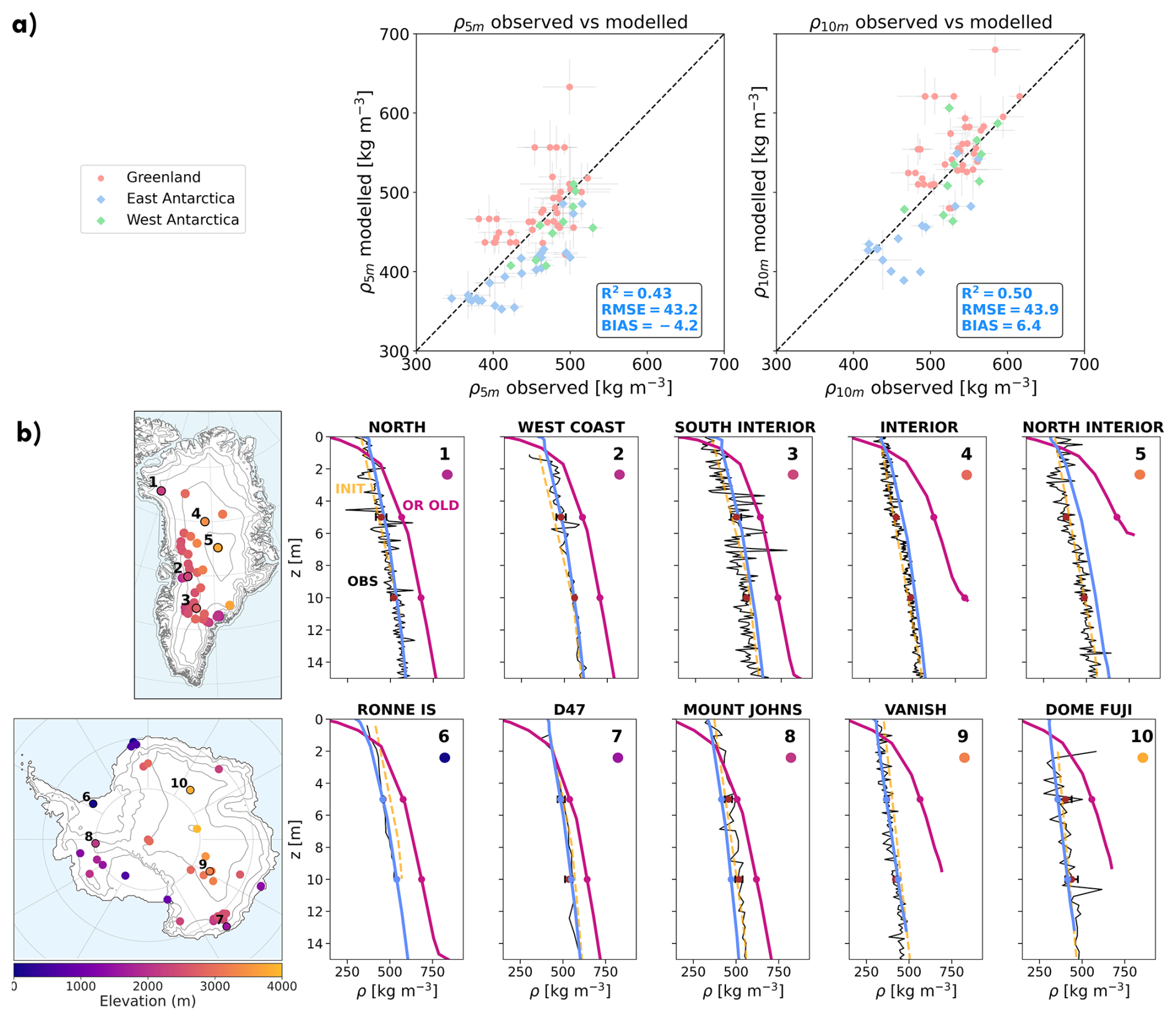
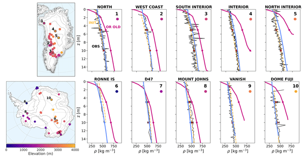
Figure 7 Comparison of (a) densities at 5 and 10 m depth between observations and the ORCHIDEE model with the calibrated set of snow viscosity parameters across both GrIS and AIS. (b) Ten density profiles representative of dry snow locations across both ice sheets. Dark lines represent observed density profiles, orange dashed lines indicate the initialization profile, the purple curves (OR OLD) show the density profile before developments and calibration and the blue ones (OR NEW) represent the new density profile. Error bars represent observational uncertainties (see Supplement).

5.2 Polar snow densification in ORCHIDEE

To assess whether the densification improvements obtained in 1D simulations extend to the ice sheet scale, we now compare modeled and observed snow densities at 5 and 10 m in 2D configurations for both ice sheets (Fig. 7). The agreement between ORCHIDEE outputs and observations is generally good. At 5 m, we note a negative bias of −4.2 kg m⁻³ (i.e. 1.1 % of the ρ_5 m average) and a RMSE of 43.2 kg m⁻³ (9.5 % with reference to the average ρ_5 m). A modest underestimation of density can be noted over Antarctica (Fig. 7a). A similar performance is obtained at 10 m with differences of 1.6 % and 8.5 % for the bias and the RMSE, respectively. These statistics demonstrate that the model reproduces the vertical structure of observed density profiles with reasonable accuracy. To further illustrate the model performance in reproducing the ρ_5 m and ρ_10 m observed metrics, we perform an evaluation over all available locations (see Figs. S1, S2 and S4 in the Supplement). Here, we selected ten dry snow observation sites (five in Greenland and five in Antarctica), chosen to cover the different regions of both ice sheets. For each location, the previous ORCHIDEE configuration is compared with the updated version of the model, including the new developments (Fig. 7b). Density profiles correspond to the annual average for the year 2019, computed from monthly outputs. Two systematic biases appear consistently across all sites when we consider the previous representation of density in ORCHIDEE (OR OLD). First, the model underestimates surface snow density by about 150 kg m⁻³. Second, it overestimates the compaction, leading to an increased density within the snowpack of around 100 to 200 kg m⁻³ compared to the observations. In the updated version of ORCHIDEE (OR NEW), these biases are considerably reduced and the vertical structure of snow density is significantly improved, despite a slight underestimation in some specific Antarctic locations such as Mount Johns (Fig. 7b).

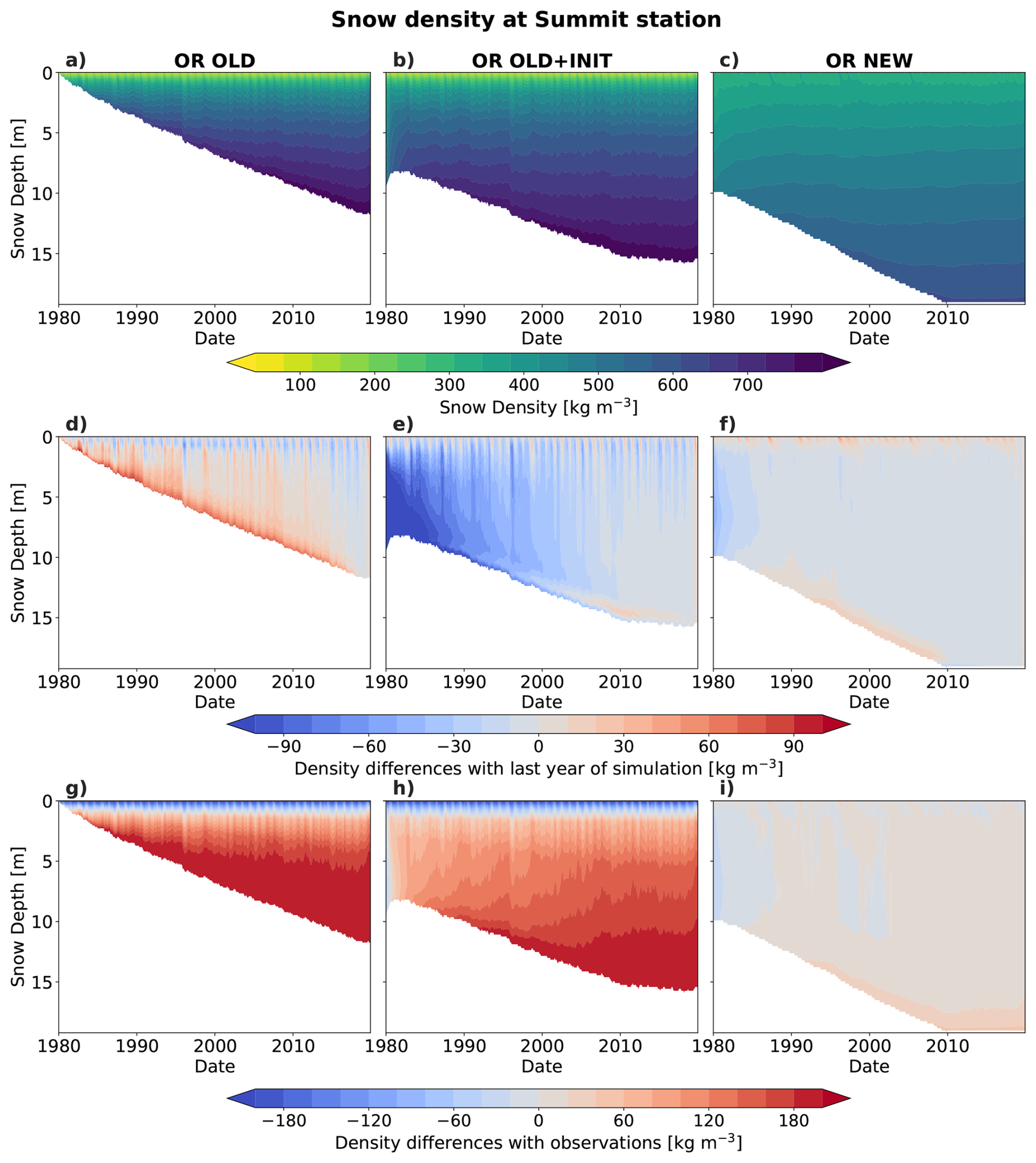
Figure 8 Monthly evolution of (a–c) the modeled snow density at Summit; (d–f) the density differences between modeled snow density and the final year averaged (2019) simulated profile, interpolated over the model snow depth at Summit for each month; and (g–i) the density differences between monthly simulated profiles and an observed density profile derived from a third-degree polynomial fit. The results are shown for three model configurations: (left) OR OLD, the previous version of ORCHIDEE, (middle) OR OLD + INIT with the initialization procedure activated, and (right) OR NEW, the final configuration with the initialization combined with the densification developments.

5.3 Effect of initialization and model developments on snow density

To investigate the effect of the initialization procedure as well as the developments proposed in this study, we choose to analyze the monthly evolution of the modeled snow density at Summit under three ORCHIDEE configurations: OR OLD, OR OLD + INIT and OR NEW described at Sect. 2.3 and Table 1. In OR OLD, it takes approximately 30 years for the model to accumulate 10 m of snow at Summit (Fig. 8a). The initialized simulation OR OLD + INIT begins with a 10 m snowpack, with an initialized steady-state density consistent with observed density profiles at Summit (Fig. 8b and h). Rapid thinning of the snowpack is observed in the first few years due to the excessive densification rate that causes OR OLD to deviate quickly from the initial density profile.

We further analyze the convergence time of the model towards its equilibrium state by considering anomalies between monthly snow density and the average profile from the final simulation year (Fig. 8d–f). In OR OLD without initialization, it takes more than 35 years to converge towards the final density profile (Fig. 8d), while OR OLD + INIT converges slightly faster, within roughly 30 years (Fig. 8e). However, OR OLD + INIT clearly diverges from the initial profile during the first decade, as indicated by the pronounced negative anomaly during this period. By the end of the simulation, the resulting density profile is significantly denser by more than 150 kg m⁻³ compared to the initialized profile, particularly in the deeper layers.

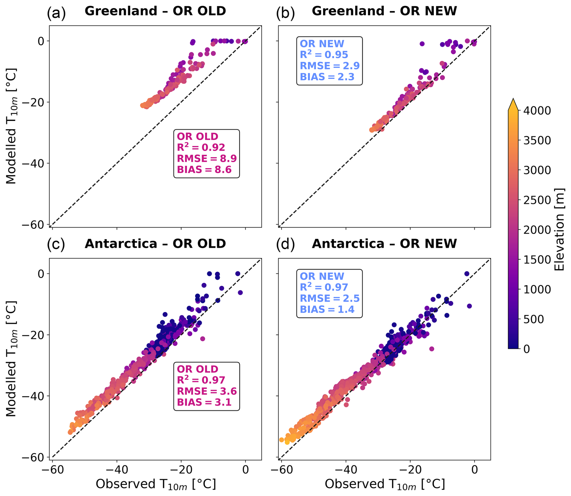
Figure 9 Comparison of observed and simulated snow temperature at 10 m depth from (a, c) the previous ORCHIDEE configuration (OR OLD) for (a) Greenland and (c) Antarctica; and from the new ORCHIDEE configuration (OR NEW) for (b) Greenland and (d) Antarctica.

Finally, when comparing monthly modeled density profiles with observed density profile at Summit (taken as the polynomial fit on the 05-2017 profile), both OR OLD and OR OLD + INIT produce too low densities near the surface (Fig. 8g and h), confirming known biases in surface densification presented in Sect. 5.1. Below the surface, the OR OLD densities are systematically too high compared to observations, regardless of the initialization (Fig. 8g and h). This confirms the excessive densification found by van Kampenhout et al. (2017) using the Anderson densification parameterization in polar regions. In contrast, the OR NEW configuration exhibits a more realistic vertical structure, with densities ranging between 300 kg m⁻³ and 600 kg m⁻³ over the top 17 m, closely matching the observed density profile (Fig. 8c and i). The bias remains below 30 kg m⁻³ through the snow column. Furthermore, OR NEW reaches equilibrium within approximately five years, substantially reducing the spin-up time (Fig. 8f). The anomaly with respect to the initial profile remains low during the entire simulation, confirming the consistency of the initialization with the long-term behavior of the model.

6 Impact of developments on temperature and melt-refreeze processes

6.1 Evaluation of the 10 m snow temperature

In the ORCHIDEE snow scheme, snow thermal conductivity and snow heat capacity are expressed as functions of density (see Sect. 2.3 and Eqs. S1–S4 in the Supplement). As a result, improvements in the representation of snow density should translate into a better representation of heat diffusion within the snowpack, and thus of the vertical temperature profile. In the following, the simulated temperature at 10 m (T_10 m), yearly averaged over the year 2019, are compared to observations using both the previous configuration (OR OLD) and the updated version (OR NEW) including all developments. In the original configuration, T_10 m is persistently overestimated across both ice sheets, with a bias of 8.6 °C in Greenland and 3.1 °C in Antarctica (Fig. 9a and c). The updated version improves the performance over Greenland and Antarctica, reducing the bias to 2.3 and 1.4 °C, respectively (Fig. 9b and d).

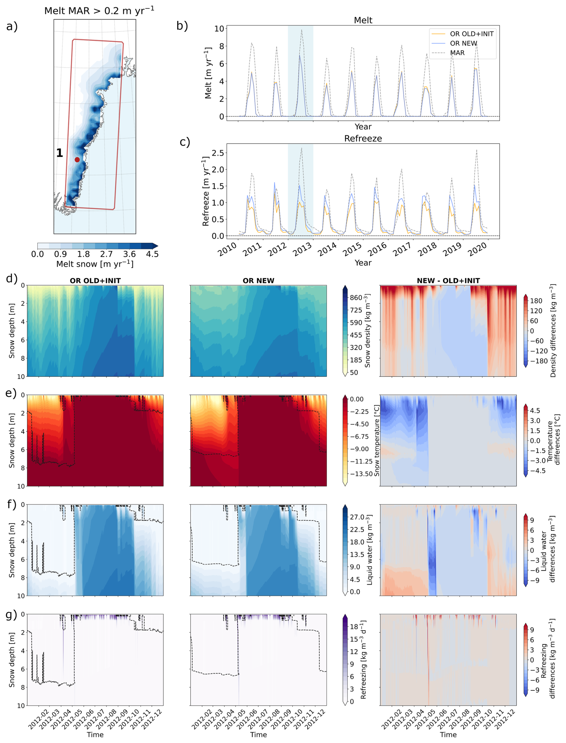
Figure 10 (a) Average melt from the MAR model over the southeast coast of the GrIS, where melt exceeds a threshold of 0.2 m yr⁻¹. (b, c) Mean seasonal melt and refreezing rates (m yr⁻¹), averaged over the region shown in (a). Results are presented for OR OLD + INIT (orange), OR NEW (blue), and MAR (dashed lines). The ORCHIDEE simulations were run using the OPT12L albedo parameters. The year 2012 is highlighted in light blue. (d–g) Simulated snow density (d), snow temperature (e), liquid water content (f), and refreezing (g), modelled with ORCHIDEE OLD + INIT (left), ORCHIDEE NEW (centre), and their differences (OR NEW − OR OLD + INIT, right). In panel (e–g), the black doted line represent the threshold where liquid water is present or not in the snowpack.

6.2 Evaluation of melt-refreeze processes

To assess the influence of our developments on modeled melt–refreezing processes in Greenland, we focus our analysis on the southeastern coast of GrIS, a region characterized by high snow accumulation and intense ablation (Fig. 10a). This area is particularly relevant for investigating refreezing dynamics, with MAR modeled mean melt rates exceeding 4.5 $\mathrm{m}{\mathrm{yr}}^{-\mathrm{1}}\mathrm{w}.\mathrm{e}.$ over 2010–2019 and recurrent episodes of strong melting and subsequent refreezing (Fig. 10b and c). Because, as presented in Sect. 2.3, the albedo parameters from Raoult et al. (2023) lead to an underestimation of melt-refreeze processes (Charbit et al., 2024), we perform the same simulations OR NEW and OR OLD + INIT with the OPT12L albedo parameters, to verify that the influence of the developments is consistent with both sets of albedo parameters. Overall, these sets of parameters lead to similar conclusions. Moreover, since our analysis focuses on melt-refreeze processes, we will use the OPT12L configuration in the following to facilitate the interpretation (Fig. 10). First we find that even with the OPT12L albedo parameters, ORCHIDEE underestimates both melt and refreezing fluxes in comparison to MAR (Fig. 10b and c). The mean seasonal melt modeled by MAR, averaged over the region presented in Fig. 10a, ranges approximately between 6.5 and almost 10 $\mathrm{m}{\mathrm{yr}}^{-\mathrm{1}}\mathrm{w}.\mathrm{e}.$ between 2010 and 2019, while ORCHIDEE values are lower by 2 to 3 $\mathrm{m}{\mathrm{yr}}^{-\mathrm{1}}\mathrm{w}.\mathrm{e}.$. Refreezing is also underestimated, with differences between OR OLD + INIT and MAR of about 0.5 to 1 $\mathrm{m}{\mathrm{yr}}^{-\mathrm{1}}\mathrm{w}.\mathrm{e}$. (Fig. 10c). Nevertheless, the updated version (OR NEW) simulates enhanced refreezing relative to the initial configuration (OR OLD + INIT).

To better understand these differences, we analyze the 2012 melt season, which featured exceptional melt events across GrIS (Fig. 10b). Although simulated melt rates are similar between OR OLD + INIT and OR NEW, refreezing differs notably early in the melt season (May–June 2012, see Fig. S8 in the Supplement). We further investigate the behavior of the model during the 2012 season at a representative site (Fig. 10a). We compare modeled snow density, temperature, liquid water, and refreezing concentration (computed, respectively as the liquid and refreezing content divided by the layer thickness). As stated previously, OR NEW corrects the underestimation of surface density and the overestimation of compaction at depth (Fig. 10d), directly influencing the snowpack temperature and liquid water content (Fig. 10e and f). Because thermal conductivity is increasing with density, the revised density profile increases snow conductivity at the surface in OR NEW. This results in a higher cold content during winter and spring, with temperature differences ranging from −1.5 to −4.5 °C between the surface and around 6 m depth (Fig. 10e). As refreezing is controlled by the available cold content, OR NEW promotes a more important refreezing of percolating meltwater (Fig. 10g). In particular, at the onset of the melt season, when the snowpack is still dry, the intense melt event of 3–14 May 2012 induces a pronounced refreezing peak, reaching 8.2 $\mathrm{kg}{\mathrm{m}}^{-\mathrm{2}}{\mathrm{d}}^{-\mathrm{1}}$ in OR NEW, nearly twice the rate in OR OLD + INIT (3.8 $\mathrm{kg}{\mathrm{m}}^{-\mathrm{2}}{\mathrm{d}}^{-\mathrm{1}}$), while the average melt amount during this melt event is similar in both simulations (12 $\mathrm{kg}{\mathrm{m}}^{-\mathrm{2}}{\mathrm{d}}^{-\mathrm{1}}\mathrm{w}.\mathrm{e}$. in OR NEW in comparison with 13.1 $\mathrm{kg}{\mathrm{m}}^{-\mathrm{2}}{\mathrm{d}}^{-\mathrm{1}}\mathrm{w}.\mathrm{e}$. in OR OLD + INIT). Throughout the melt season, refreezing rates near the surface remain consistently higher in OR NEW, with differences on the order of 8 to 10 $\mathrm{kg}{\mathrm{m}}^{-\mathrm{3}}{\mathrm{d}}^{-\mathrm{1}}$ (Fig. 10g). This increased refreezing in OR NEW directly lowers the liquid water content compared to OR OLD + INIT, as observed in May 2012 (Fig. 10f) with differences of −6 to −9 kg m⁻³ between 4 and 10 m depth.

In conclusion, the new developments promote higher refreezing rates by modifying the snow density and viscosity profiles. In OR OLD + INIT, the snowpack remains almost too warm to refreeze additional meltwater. In contrast, the colder snowpack in OR NEW allows for greater refreezing potential, which is consistent with the need to increase the melt and refreeze content in line with MAR.

6.3 Densification in the lower percolation zone

As shown previously, compared with MAR, ORCHIDEE underestimates refreezing within the snowpack, due to an underestimation of meltwater production. This has an impact on densification in the Greenland lower percolation zone, defined generally as the low elevation area of the ice sheet where annual snow melt exceeds accumulation. Indeed, the resulting meltwater significantly influences water percolation and thus refreezing within the snowpack, which in turn affects densification.

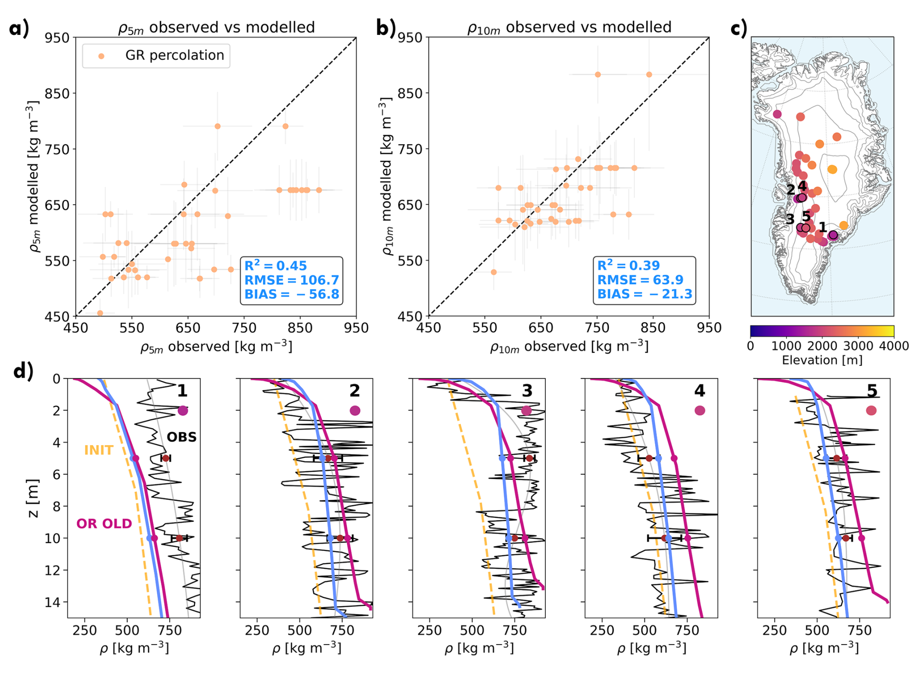
Figure 11 Observed density at 5 m ρ_5 m (a) and 10 m ρ_10 m (b) compared to modeled ones with the new viscosity parameters across the Greenland percolation locations. (c) Locations of the five profiles selected. (d) Density profiles representatives of percolation locations across Greenland. Dark lines represent observed density profiles (OBS), orange dashed line the initialization profile (INIT), the purple curve the ORCHIDEE density profile before developments (OR OLD) and the blue curve with the new ORCHIDEE configuration (OR NEW). Locations of the five density profiles are shown in (c). Error bars represent observational uncertainties (see Supplement).

In the lower percolation zone, ORCHIDEE underestimates snow density at both 5 and 10 m (Fig. 11a), with a larger bias at 5 m (−56.8 kg m⁻³) than at 10 m (−21.3 kg m⁻³). At 10 m, the influence of refreezing on densification diminishes, as the water does not percolate significantly at this depth, and the compaction becomes the dominant densification process. Since the compaction scheme was calibrated using dry snow conditions, where refreezing is negligible, the model performs more accurately at 10 m. These results likely indicate that accurate representation of density in the percolation zones may depend on the ability of the model to simulate melt and refreeze processes.

Further qualitative analysis is done by comparing observed and modeled density profiles from ORCHIDEE in the percolation zone (Fig. 11d). The profiles 2–5 show some successful reproduction of densification trends in this area. Exception is made for the first profile, which represents a modeled snowpack without clear evidence of refreezing (with surface densities around 600 kg m⁻³), whereas density observations suggest that refreezing occurs, leading to a densification of the snowpack. Other available observed profiles can be found in Figs. S1–S3 in the Supplement and show similar results.

7 Discussion and conclusion

We have introduced a series of model developments in ORCHIDEE aimed at improving the representation of polar snow density over the Greenland and Antarctic ice sheets. The model performance has been evaluated through offline experiments and compared against in situ observations.

We first proposed a new initialization procedure for the snowpack over polar ice sheets. This method allows to start the simulations with a prescribed snow depth and a vertical density structure consistent with field observations. This method induces a substantial reduction in spin-up duration, which is especially valuable for coupled atmosphere-surface simulations. By relying only on latitude and surface elevation to reconstruct the density profile, this approach is aimed to be generalizable to any polar snowpack model.

In addition, we introduced in the ORCHIDEE model a new empirical parameterization of surface snow density for polar regions, which is valid for both ice sheets and based on the 10 m wind speed. It has been calibrated using the wind speed weighted by precipitation against surface density observations. This formulation is a pragmatic approach to represent the rapid surface densification processes that are not explicitly represented in the model. Enhancing wind densification is considered a temporary solution, pending a better understanding and representation of the physical processes controlling surface snow densification. As an example, saltation, a process not captured by ORCHIDEE, can be an important driver of surface densification due to the mechanical impacts on the snowpack when snow crystals fall onto the surface (Sommer et al., 2017; Walter et al., 2024). To compensate for unresolved processes, similar wind-based strategies have also been adopted in other regional models, such as MAR (Kittel et al., 2021) and the IMAU-Firn densification model (IMAU-FDM; Lenaerts et al., 2012; Veldhuijsen et al., 2023). Moreover, the comparison with surface snow density observations shows that the proposed parameterization successfully corrects the large underestimation present over polar regions in the previous model version.

Finally, we calibrated the viscosity parameters from the Anderson (1976) densification equation (Eq. 2). Using the History Matching procedure, we achieved a significantly improved representation of snow compaction in dry-snow conditions. These new viscosity parameters enable to reduce the overestimated compaction previously identified in ORCHIDEE in various locations of the GrIS and AIS. They also contribute to a reduction of the snow temperature bias in the model. However, this improvement still does not fully capture densification in ablation areas, where refreezing of percolated liquid water drives additional densification, especially in the first meters of the snowpack. As discussed in Sect. 6.2, both meltwater production and refreezing remain underestimated in ORCHIDEE. Therefore, accurately representing the percolation zone relies on correctly simulating these melting and refreezing cycles and, by extension, the meltwater infiltration within the snowpack. Different field studies suggest that meltwater infiltration can occur through different mechanisms, either forming a uniform advance of a wetting front or through localized preferential flow paths (Marsh and Woo, 1984; Pfeffer and Humphrey, 1996). However, the mechanisms of infiltration remain insufficiently observed. Complex models that include a representation of both types of flow tend to overestimate the depth of penetration, while bucket schemes appear to underestimate it (Vandecrux et al., 2020). As recommended in this study, field campaigns combined with laboratory experiments are needed to better constrain the conditions of meltwater infiltration. Considering the influence of the liquid water retention capacity formulation (following the approach of Lafaysse et al., 2017) may be an effective step towards a better representation of liquid water retention and refreezing processes in ORCHIDEE. Indeed, alternative formulations (Lafaysse et al., 2017) simulate the opposite behavior as the formulation implemented in ORCHIDEE and have been shown to be consistent with laboratory experiments (Coléou and Lesaffre, 1998). Exploring the sensitivity of the model to these different parameterizations may help assess their impact on the simulation of refreezing processes.

Another perspective to improve the simulation of meltwater production, and therefore refreezing, is to focus on the representation of the surface energy balance, with particular attention to the snow albedo parameterization and surface fluxes such as latent and sensible heat fluxes. This perspective will be explored using coupled experiments in order to capture surface/atmosphere feedbacks, particularly important for the albedo modeling. Special emphasis will be placed on refining the current simplified albedo formulation (Chalita and Le Treut, 1994), which represents albedo as a time-evolving function of snow age. Yet, the snow microstructure has a significant influence on snow spectral albedo (Skiles et al., 2018). This underlines the need for an explicit representation of the specific surface area in order to have a more physically based albedo scheme. Pending this development, an alternative approach consists of introducing different albedo decay rates for dry and wet snow in the current albedo parameterization, inspired by Helsen et al. (2017). This can be a step towards a better representation of the albedo decay rate during the melt season. Nevertheless, the developments presented in this paper improve significantly the representation of snowpack internal processes and are a key milestone for a more accurate assessment of the surface mass balance of polar ice sheets in the IPSL climate model.

Appendix A: Snowpack Initialization

We propose an explicit formulation for the density ρ after integration of the Ligtenberg et al. (2011) equation along the vertical axis, expressed as a differenced function based on the critical depth z₅₅₀ where ρ equals 550 kg m⁻³:

$$\begin{array}{}\text{(A1)}& {\displaystyle }\mathit{\rho }={\displaystyle \frac{\exp \left(E_{\mathrm{0}}\left(\stackrel{\mathrm{‾}}{T_{\mathrm{s}}}\right)z\right)}{\frac{{\mathit{\rho }}_i}{{\mathit{\rho }}_{\mathrm{s}}}-\mathrm{1}+\exp \left(E_{\mathrm{0}}\left(\stackrel{\mathrm{‾}}{T_{\mathrm{s}}}\right)z\right)}}{\mathit{\rho }}_i\text{ if }z<z_{\mathrm{550}}\text{(A2)}& {\displaystyle }\mathit{\rho }={\displaystyle \frac{\exp \left(E_{\mathrm{1}}\left(\stackrel{\mathrm{‾}}{T_{\mathrm{s}}}\right)(z-z_{\mathrm{550}})\right)}{\frac{{\mathit{\rho }}_i}{\mathrm{550}.}-\mathrm{1}+\exp \left(E_{\mathrm{1}}\left(\stackrel{\mathrm{‾}}{T_{\mathrm{s}}}\right)(z-z_{\mathrm{550}})\right)}}{\mathit{\rho }}_i\text{ if }z>z_{\mathrm{550}}\end{array}$$

Here, ρ_s refers to the surface density in kg m⁻³, $E_{\mathrm{0}}\left(\stackrel{\mathrm{‾}}{T_{\mathrm{s}}}\right)=C_{\mathrm{0}}g\exp \left(\frac{E_{\mathrm{g}}-E_{\mathrm{c}}}{R\stackrel{\mathrm{‾}}{T_{\mathrm{s}}}}\right)\mathit{\gamma }$ and $E_{\mathrm{1}}\left(\stackrel{\mathrm{‾}}{T_{\mathrm{s}}}\right)=C_{\mathrm{1}}g{\mathit{\rho }}_i\exp \left(\frac{E_{\mathrm{g}}-E_{\mathrm{c}}}{R\stackrel{\mathrm{‾}}{T_{\mathrm{s}}}}\right)\mathit{\gamma }$, where $\mathit{\gamma }=\mathit{\alpha }\ln \left(\stackrel{\mathrm{‾}}{A}\right)$ is the correction term defined previously in Sect. 3.1 (see Eq. 6), and C₀=0.03 and C₁=0.07 are the constants introduced in Eq. (5).

To derive a density parameterization that depends only on latitude and elevation, we aim to parameterize three key variables required in formulations (A1) and (A2) : the average surface temperature $\stackrel{\mathrm{‾}}{T_{\mathrm{s}}}$, the logarithm of the average annual accumulation rate $\ln \left(\stackrel{\mathrm{‾}}{A}\right)$, and the surface density ρ_s. These parameterizations are based on physical considerations and empirical relationships between these variables and surface elevation and latitude.

First, we introduce a parameterization for the mean surface temperature as a function of latitude and elevation, following the elevational lapse rates identified by Feulner et al. (2013) for Antarctica and by Hanna et al. (2005) for Greenland. Next, we define a parameterization for the logarithm of the mean accumulation rate $\ln (\stackrel{\mathrm{‾}}{A}$) as a function of the mean annual surface temperature, based on the Clausius-Clapeyron relationship. Furthermore, we establish a parameterization for the surface density assuming a linear relationship between the surface density and the mean annual surface temperature. Finally, we introduce a varying snowpack thickness parameterization defined as a function of snow temperature. Each parameterization is defined separately for Greenland and Antarctica, with the exception of the snowpack thickness parameterization introduced for Greenland only.

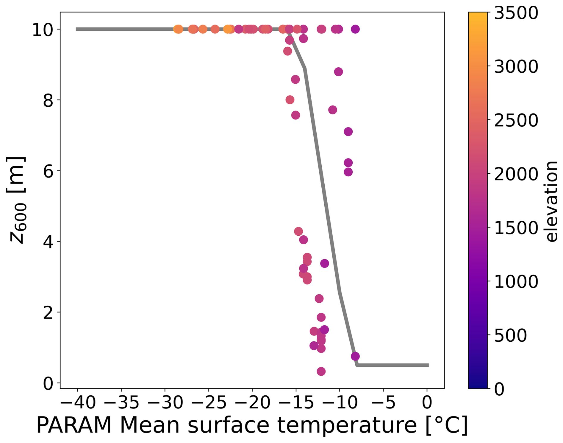
Figure A1 Observed snowpack thickness at which 600 kg m⁻³ is reached (z₆₀₀) as a function of the parameterized mean surface temperature and surface elevation, in Greenland. The grey line represents the parameterization of mean snowpack thickness as a function of the parameterized mean surface temperature.

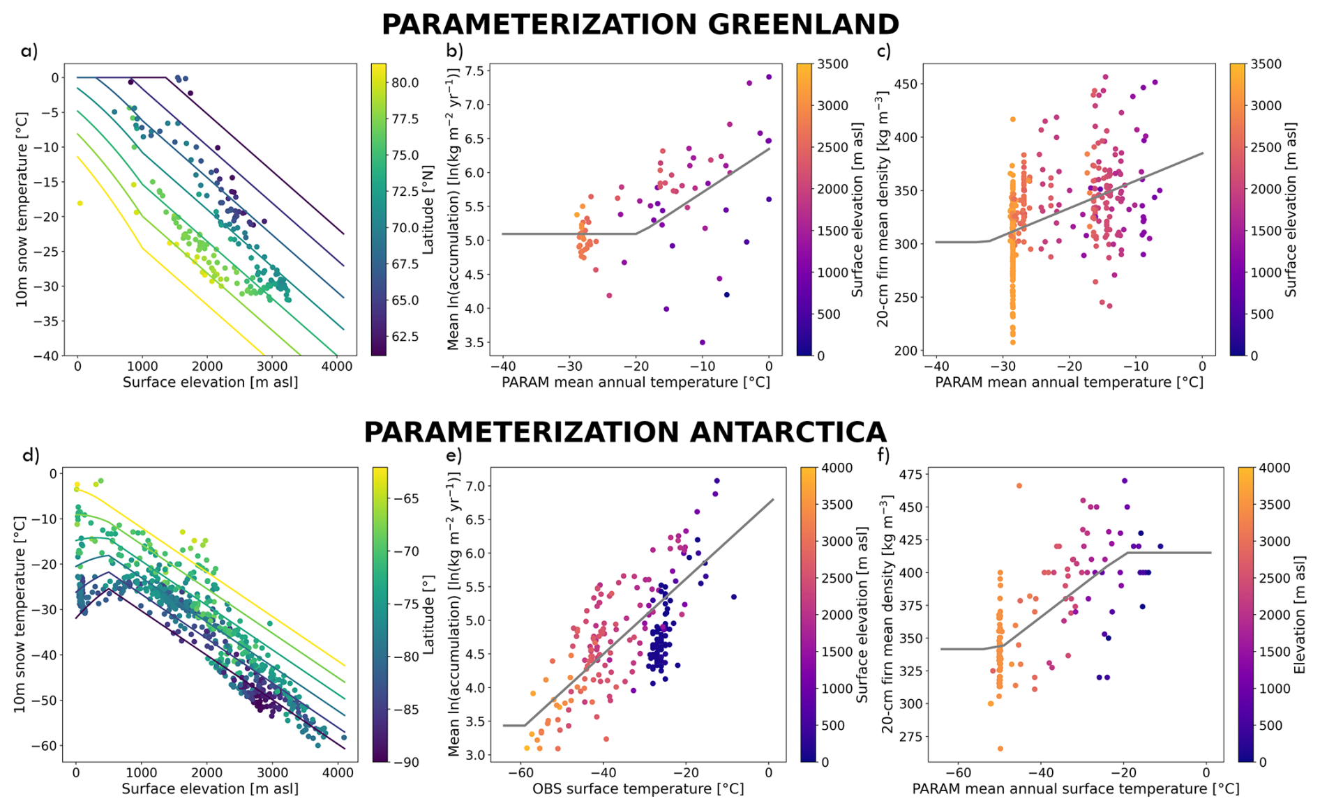
Figure A2 Observed 10 m snow temperature in function of surface elevation and latitude in Greenland (a) and Antarctica (d). Colored lines represent the parameterization of mean annual surface temperature in function of latitude and elevation. Logarithm accumlation observations in function of the parameterized mean annual surface temperature and surface elevation in Greenland (b) and Antarctica (e). Grey line show the final parameterization in function of the parameterized mean annual surface temperature. Surface density observations in function of the parameterized mean surface temperature and surface elevation in Greenland (c) and Antarctica (f). Grey line shows the parameterized surface density in function of the parameterized mean annual surface temperature.

A1 Parameterization of mean surface temperature $\stackrel{\mathrm{‾}}{T_{\mathrm{s}}}$

To parameterize the mean surface temperature, we base our approach on the theoretical temperature gradients with respect to altitude and latitude for Antarctica (AIS) and Greenland (GrIS). For the AIS, we adopted the dry-adiabatic lapse rate with respect to altitude, proposed by Feulner et al. (2013) and equal to 9.8 °C km⁻¹. In our approach, we distinguished the temperature gradient with elevation and latitude based on a critical altitude of 500 m above sea level (h₅₀₀). This threshold distinguishes two distinct regimes observed in the tendencies of the 10 m snow temperature in the AIS (Fig. A2): a first tendency for elevation lower than 500 $\mathrm{m}\mathrm{a}.\mathrm{s}.\mathrm{l}.$ taking into account ice shelves and the second regime associated to the rest of the ice sheet. The lower temperature lapse rate was prescribed to 6.5 °C km⁻¹ for elevations below 500 m. This value was obtained using the Broyden–Fletcher–Goldfarb–Shanno (BFGS) optimization algorithm to minimize the root mean square error between the parameterized mean surface temperature and the observed firn temperature at a depth of 10 m. For the GrIS, we followed the theoretical lapse rate with respect to elevation proposed by Hanna et al. (2005) equal to 5.9 °C km⁻¹ below 1000 $\mathrm{m}\mathrm{a}.\mathrm{s}.\mathrm{l}.$ (h₁₀₀₀) and 8.2 °C km⁻¹ above this critical altitude. The dependency of the mean surface temperature on latitude is based on an empirical relationship in order to represent the decrease of temperature towards the pole. To determine this temperature gradient, we applied the same minimization procedure as described above, using the BFGS optimization algorithm.

We obtain the following temperature gradients with respect to latitude, resulting from the optimization and with respect to elevation based on the considerations of Feulner et al. (2013) and Hanna et al. (2005). For AIS:

$$\begin{array}{}\text{(A3)}& \left\{\begin{array}{l}\begin{array}{c}{\frac{\mathrm{\Delta }T}{\mathrm{\Delta }\text{lat}}}_{\text{low\hspace{0.17em}\hspace{0.17em}alt}}=\mathrm{1.14}\mathrm{°}\mathrm{C}{\mathrm{lat}}^{-\mathrm{1}},{\frac{\mathrm{\Delta }T}{\mathrm{\Delta }z}}_{\text{low\hspace{0.17em}\hspace{0.17em}alt}}=\mathrm{6.5}\mathrm{°}\mathrm{C}{\mathrm{km}}^{-\mathrm{1}}\\ \text{if }z<h_{\mathrm{500}}\mathrm{m}\mathrm{a}.\mathrm{s}.\mathrm{l}.,\end{array}\\ \begin{array}{c}{\frac{\mathrm{\Delta }T}{\mathrm{\Delta }\text{lat}}}_{\text{high\hspace{0.17em}\hspace{0.17em}alt}}=\mathrm{0.73}\mathrm{°}\mathrm{C}{\mathrm{lat}}^{-\mathrm{1}},{\frac{\mathrm{\Delta }T}{\mathrm{\Delta }z}}_{\text{high\hspace{0.17em}\hspace{0.17em}alt}}=\mathrm{9.8}\mathrm{°}\mathrm{C}{\mathrm{km}}^{-\mathrm{1}}\\ \text{if }z\ge h_{\mathrm{500}}\mathrm{m}\mathrm{a}.\mathrm{s}.\mathrm{l}.\end{array}\end{array}\right.\end{array}$$

For GrIS:

$$\begin{array}{}\text{(A4)}& \left\{\begin{array}{l}\begin{array}{c}{\frac{\mathrm{\Delta }T}{\mathrm{\Delta }\text{lat}}}_{\text{low\hspace{0.17em}\hspace{0.17em}alt}}=-\mathrm{0.66}\mathrm{°}\mathrm{C}{\mathrm{lat}}^{-\mathrm{1}},{\frac{\mathrm{\Delta }T}{\mathrm{\Delta }z}}_{\text{low\hspace{0.17em}\hspace{0.17em}alt}}=\mathrm{5.9}\mathrm{°}\mathrm{C}{\mathrm{km}}^{-\mathrm{1}}\\ \text{if }z<h_{\mathrm{1000}}\mathrm{m}\mathrm{a}.\mathrm{s}.\mathrm{l}.,\end{array}\\ \begin{array}{c}{\frac{\mathrm{\Delta }T}{\mathrm{\Delta }\text{lat}}}_{\text{high\hspace{0.17em}\hspace{0.17em}alt}}=-\mathrm{0.92}\mathrm{°}\mathrm{C}{\mathrm{lat}}^{-\mathrm{1}},{\frac{\mathrm{\Delta }T}{\mathrm{\Delta }z}}_{\text{high\hspace{0.17em}\hspace{0.17em}alt}}=\mathrm{8.2}\mathrm{°}\mathrm{C}{\mathrm{km}}^{-\mathrm{1}}\\ \text{if }z\ge h_{\mathrm{1000}}\mathrm{m}\mathrm{a}.\mathrm{s}.\mathrm{l}.\end{array}\end{array}\right.\end{array}$$

We express the parameterization of mean annual surface temperature as follows, depending on the temperature gradient with respect to latitude and elevation:

$$\begin{array}{}\text{(A5)}& {\displaystyle }\begin{array}{rl}{\displaystyle \frac{\mathrm{\Delta }T}{\mathrm{\Delta }\text{lat}}}\left(z\right)=& \left({\displaystyle \frac{{\frac{\mathrm{\Delta }T}{\mathrm{\Delta }\text{lat}}}_{\text{high\hspace{0.17em}\hspace{0.17em}alt}}-{\frac{\mathrm{\Delta }T}{\mathrm{\Delta }\text{lat}}}_{\text{low\hspace{0.17em}\hspace{0.17em}alt}}}{z_{\text{high\hspace{0.17em}\hspace{0.17em}alt}}-z_{\text{low\hspace{0.17em}\hspace{0.17em}alt}}}}\right)\\ & \times (z-z_{\text{low\hspace{0.17em}\hspace{0.17em}alt}})+{{\displaystyle \frac{\mathrm{\Delta }T}{\mathrm{\Delta }\text{lat}}}}_{\text{low\hspace{0.17em}\hspace{0.17em}alt}}\end{array}\text{(A6)}& {\displaystyle }\begin{array}{rl}{\displaystyle \frac{\mathrm{\Delta }T}{\mathrm{\Delta }z}}\left(z\right)=& \left({\displaystyle \frac{{\frac{\mathrm{\Delta }T}{\mathrm{\Delta }z}}_{\text{high\hspace{0.17em}\hspace{0.17em}alt}}-{\frac{\mathrm{\Delta }T}{\mathrm{\Delta }z}}_{\text{low\hspace{0.17em}\hspace{0.17em}alt}}}{z_{\text{high\hspace{0.17em}\hspace{0.17em}alt}}-z_{\text{low\hspace{0.17em}\hspace{0.17em}alt}}}}\right)\\ & \times (z-z_{\text{low\hspace{0.17em}\hspace{0.17em}alt}})+{{\displaystyle \frac{\mathrm{\Delta }T}{\mathrm{\Delta }z}}}_{\text{low\hspace{0.17em}\hspace{0.17em}alt}}\end{array}\text{(A7)}& {\displaystyle }\begin{array}{rl}{T}_{\mathrm{s}}(\text{lat},z)=& min({\displaystyle \frac{\mathrm{\Delta }T}{\mathrm{\Delta }\text{lat}}}\cdot (\text{lat}-{\text{lat}}_{\text{ref}})-{\displaystyle \frac{\mathrm{\Delta }T}{\mathrm{\Delta }z}}\\ & \times {\displaystyle \frac{(z-z_{\text{ref}})}{\mathrm{1000}}}+T_{\text{s\_ref}},\mathrm{0})\end{array}\end{array}$$

The parameters used in the surface temperature parameterization for Antarctica and Greenland can be found in the following table.

Table A1 Parameters used in the surface temperature parameterization. MBE and RMSE are the mean bias error and root mean square error, respectively. MBE (Obs) and RMSE (Obs) correspond to the comparison between observed temperatures and the parameterized temperature using the elevation and latitude of the observations. MBE (MAR) and RMSE (MAR) are computed similarly, but using the mean 10 m snow temperature field from MAR over 1980–2019, compared to the parameterized temperature evaluated at the elevation and latitude of each MAR grid point.

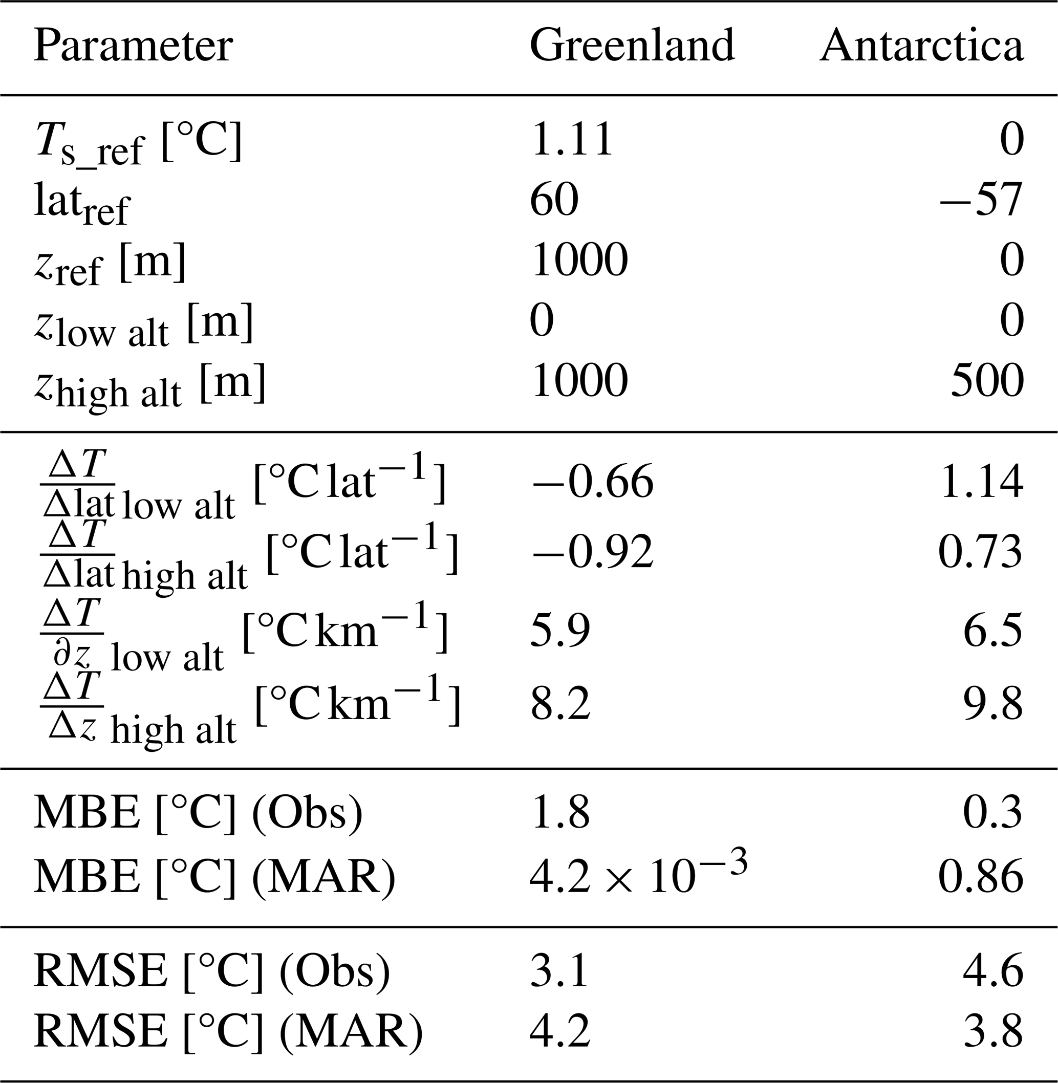
A2 Parameterization of mean logarithm accumulation $\ln \left(\stackrel{\mathrm{‾}}{A}\right)$

To estimate the logarithm of accumulation ($\ln \left(\stackrel{\mathrm{‾}}{A}\right)$) in Eqs. (A1) and (A2), we define a linear relationship with the mean annual surface temperature, according to the Clausius Clapeyron law. In Antarctica (AIS), accumulation records also include surface temperature measurements. These are used to calibrate the dependence of $\ln \left(\stackrel{\mathrm{‾}}{A}\right)$ on surface temperature. For Greenland, no such temperature data are available. Nevertheless, the surface elevation and latitude at the observation sites allow us to compute the parameterized mean surface temperature, as defined earlier.

We derive the following expression to parameterize $\ln \left(\stackrel{\mathrm{‾}}{A}\right)$ in function of the mean annual surface temperature T_s:

$$\begin{array}{}\text{(A8)}& \begin{array}{rl}\ln \left(\stackrel{\mathrm{‾}}{A}\right)=& max({\displaystyle \frac{\mathrm{\Delta }\ln \left(\stackrel{\mathrm{‾}}{A}\right)}{\mathrm{\Delta }{T}_{\mathrm{s}}}}\cdot (T_{\mathrm{s}}-T_{s\mathit{\_}\text{ref}})\\ & +\ln \left({\stackrel{\mathrm{‾}}{A}}_{\text{ref}}\right),\ln \left({\stackrel{\mathrm{‾}}{A}}_{min}\right))\end{array}\end{array}$$

Table A2 Parameters used in the logarithm of the accumulation parameterization. MBE and RMSE are the mean bias error and root mean square error, respectively. MBE (Obs) and RMSE (Obs) correspond to the comparison between the observations of the logarithm of accumulation and the parameterized logarithm of the accumulation. MBE (MAR) and RMSE (MAR) are computed similarly, but using the mean logarithm of the accumulation from MAR over 1980–2019, compared to the parameterized logarithm of the accumulation evaluated for each MAR grid point.

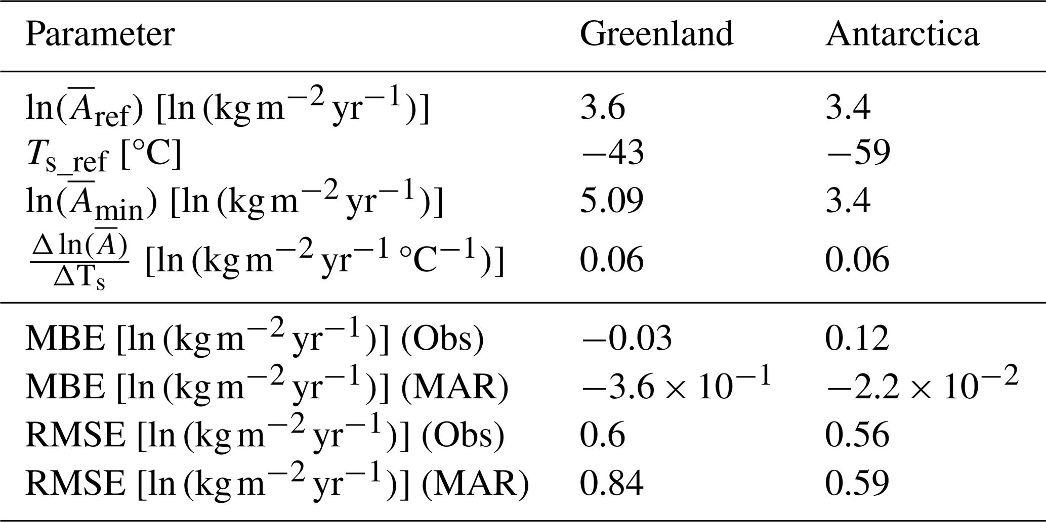
The BFGS optimization algorithm is used to determine the optimal rate of variation of the mean logarithm accumulation with respect to the parameterized mean surface temperature. This optimization process aims to minimize the RMSE between the observed and parameterized mean logarithm of accumulation (Fig. A2). The optimized parameters used in the logarithm of the accumulation parameterization can be found in Table A2.

A3 Parameterization of surface density ρ_s

In this study, for the initialization, we choose to define an empirical linear relationship between the observed surface density and the mean annual surface temperature, derived from the parameterization based on latitude and elevation.

$$\begin{array}{}\text{(A9)}& \begin{array}{rl}{\mathit{\rho }}_{\mathrm{s}}\left(T_{\mathrm{s}}\right)=& min(max(\left({\displaystyle \frac{{\mathit{\rho }}_{\mathrm{2}}-{\mathit{\rho }}_{\mathrm{1}}}{T_{\mathrm{2}}-T_{\mathrm{1}}}}\right)(T_{\mathrm{s}}-T_{\mathrm{1}})\\ & +{\mathit{\rho }}_{\mathrm{1}},{\mathit{\rho }}_{\text{s\_min}}),{\mathit{\rho }}_{\text{s\_max}})\end{array}\end{array}$$

The empirical relationship between observed surface density and parameterized surface temperature is then optimized by the BFGS algorithm, separately for Greenland and Antarctica, in order to minimize the RMSE between observed and parameterized surface density. The parameters used in the surface snow density parameterization can be found in Table A3.

Table A3 Parameters used in the snow density parameterization.

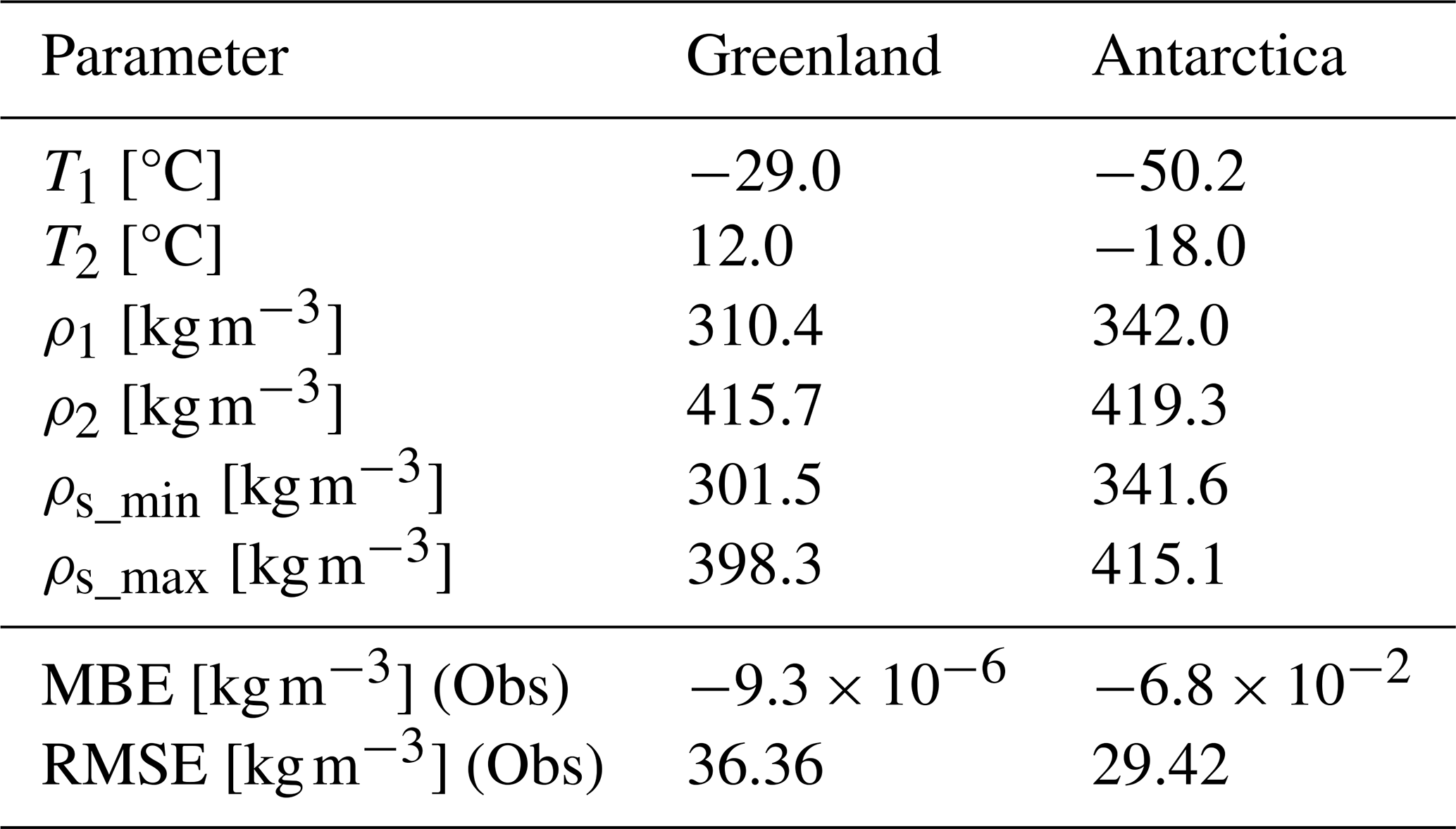
A4 Parameterization of the snowpack thickness

Our initialization routine allows us to create a snowpack of a uniform thickness with consistent dry snow density properties for the GrIS and AIS. Initializing snowpack thickness can have an influence on the amount of modeled snow melt volumes. A uniform snowpack thickness across all regions can introduce biases, especially in areas where the snowpack is naturally thin due to recurrent melt events. This is a concern for the percolation and ablation zones of the GrIS. We introduce a variable snowpack thickness in order to better represent these ablation zones of the GrIS. As ablation areas are overall not a concern in Antarctica, this development only applies to the GrIS.

We base our approach on observed density profiles, specifically looking at the depth where a density of 600 kg m⁻³ (dz₆₀₀) is reached. This threshold is arbitrary and serves only to differentiate ablation zones from dry snow areas. Percolation and ablation zones are characterized by melting and refreezing processes, leading to a thinner snowpack that densifies quickly in comparison to dry snow locations. Thus, with this criteria dz₆₀₀ we can differentiate the percolation and ablation zones from the dry snow zones, where densification is slower and less affected by melt-refreeze cycles. After calculating the indicator dz₆₀₀ from density profile trends (to minimize observational noise), we extract the parameterized temperature at the observed points and define the parameterization for snowpack thickness as a function of this variable (Fig. A1).

$$\begin{array}{}\text{(A10)}& \begin{array}{rl}{z}_{\text{snow}}\left(T_{\mathrm{s}}\right)=& min(max(z_{\text{snow}\mathrm{2}}-\left({\displaystyle \frac{z_{\text{snow}\mathrm{2}}-z_{\text{snow}\mathrm{1}}}{T_{\text{s2}}-T_{\text{s1}}}}\right)\\ & \times (T_{\mathrm{s}}-T_{\text{s1}}),z_{\text{snow\_min}}),z_{\text{snow\_max}}y)\end{array}\end{array}$$

This results in a parameterization that allows us to distinguish at the initialization the snowpack thickness of the ablation and percolation zone from the rest of the GrIS. The parameters used for the snowpack thickness over Greenland are presented in Table A4.

Table A4 Parameters for the snow thickness parameterization (Greenland only).

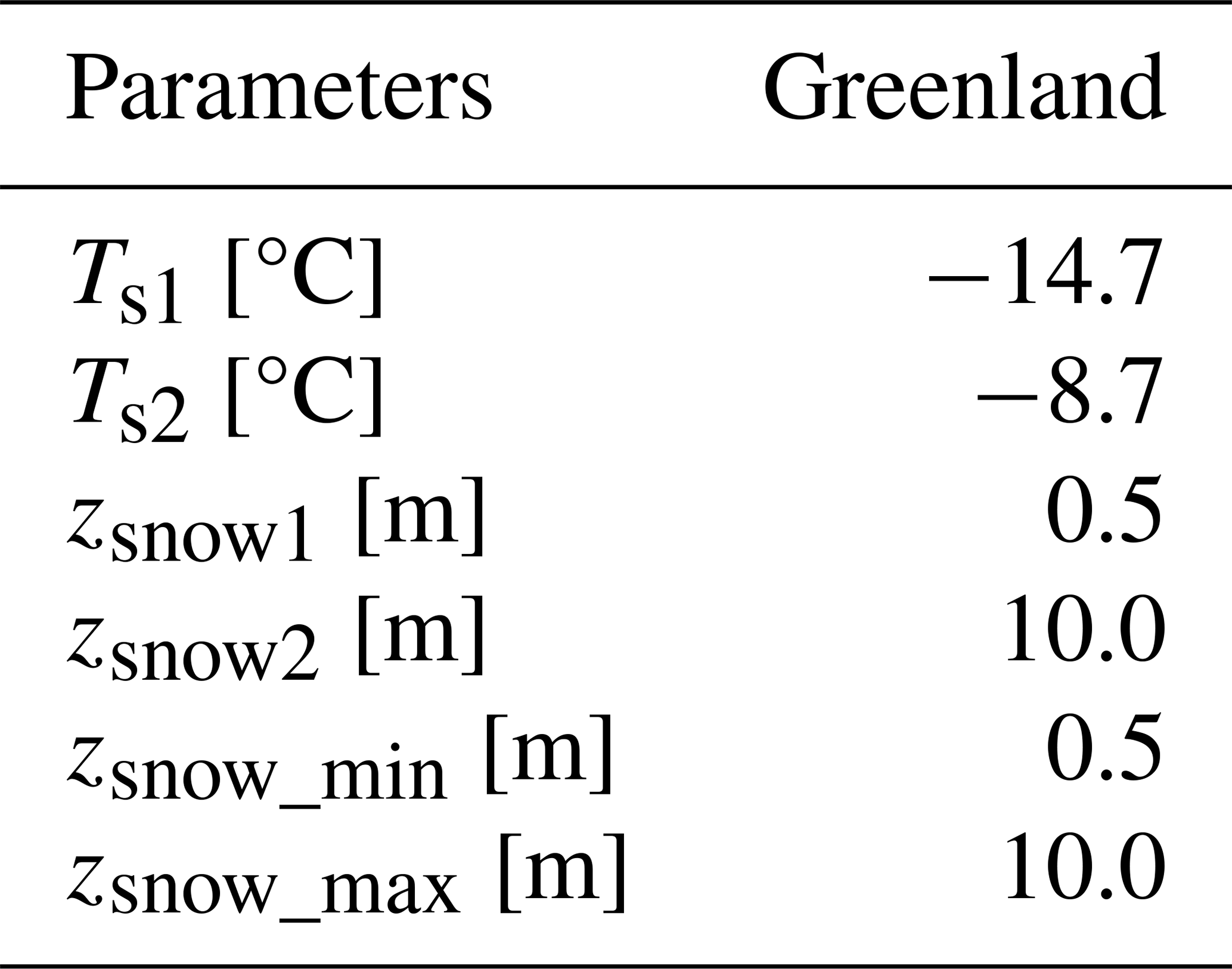
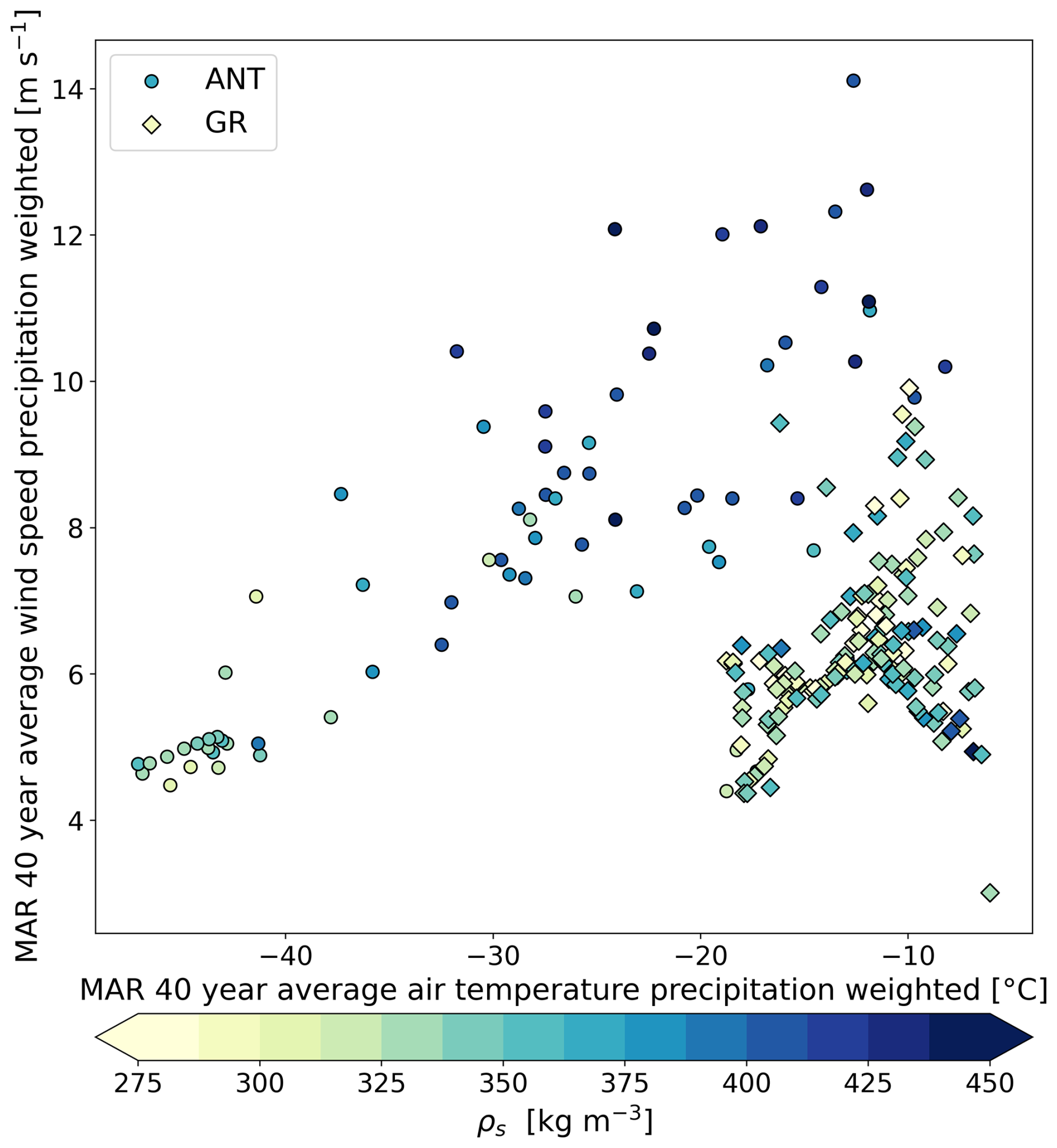
Figure A3 Comparison of observed surface snow density in Antarctica (circle) and Greenland (diamond) as a function of MAR 40 years (1980–2019) average precipitation-weighted air temperature (x-axis) and precipitation-weighted wind speed (y-axis).

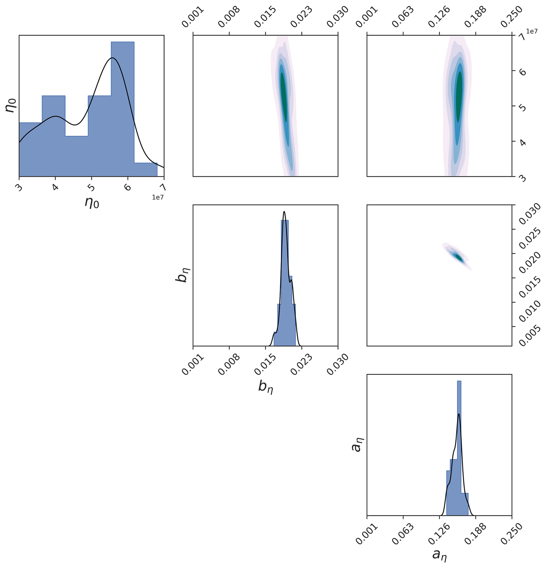
Figure A4 Marginal (diagonal) and joint (off-diagonal) distributions of the 30 sets of viscosity parameters (η₀, b_η, and a_η) of the fifth History Matching wave.