Year-Round High-Resolution Sea Ice Freeboard Retrieval Using ICESat-2 ATL03 Photon Data

Arctic sea ice freeboard is critical for estimating ice thickness and characterizing surface morphology, yet it remains poorly constrained, especially during the melt season due to limitations in conventional altimetry products. The ICESat-2 ATL07 product retrieves surface heights using variable along-track segment lengths (10–200 m) and identifies floes and leads using fixed thresholds based on photon rate, background rate, and width of the photon distribution to support freeboard estimation. This strategy can smooth ice-ridge-related features and reduce reliability over sea-ice surfaces with complex spatial variations or melt-affected conditions. To address these challenges, we present a year-round, high-resolution (5 m) freeboard retrieval method (HRFM) based directly on ICESat-2 ATL03 photon data. A two-stage denoising strategy is implemented to robustly extract signal photons, while a machine-learning classifier, trained using 25 coincident Sentinel-2/ICESat-2 scenes, discriminates between sea ice, thin ice, and leads under both winter and summer surface conditions. Identified lead segments are used to construct local sea-surface references for freeboard estimation. Validation against Airborne Topographic Mapper (ATM) data shows that HRFM reduces the surface-height root-mean-square error (RMSE) for strong beams from 0.12 m (ATL07) to 0.08 m (by 33 %). HRFM better preserves ridge-related heights that are smoothed in ATL07. The classifier attains a precision of 0.96 and a recall of 0.95 for lead detection, supporting reliable freeboard estimation. Weak-beam retrievals also show encouraging validation performance under the same evaluation framework. During the 1-year demonstration period, the spatial patterns of retrieved freeboard are broadly consistent with the ICESat-2 ATL20 product, while monthly mean differences between the two products reach up to 0.04 m. By improving topographic fidelity and lead detection, HRFM provides a framework for high-resolution freeboard retrieval under both winter and summer surface conditions.

1 Introduction

Arctic sea ice plays a pivotal role in regulating exchanges of heat (Aylmer et al., 2024), momentum (Muilwijk et al., 2024), and water vapor (Ridley et al., 2023) between the atmosphere and oceans, with impacts spanning local processes to the global climate system (Sun et al., 2018). Changes in sea-ice thickness are widely recognized as a key indicator of climate change (Stroeve and Notz, 2018), influencing the surface energy balance (von Schuckmann et al., 2023; Zhou et al., 2025), ocean–atmosphere interactions (McPhee, 2008; Timmermans and Marshall, 2020), high-latitude biodiversity (Macias-Fauria and Post, 2018; Pratte et al., 2019), and Arctic shipping operations (Shu et al., 2024). Sea-ice freeboard, defined as the height of the ice surface above the local sea level, is a fundamental parameter for estimating ice thickness from satellite altimeters (Kacimi and Kwok, 2024), for characterizing surface roughness relevant to stress and momentum transfer (Krumpen et al., 2025; Mchedlishvili et al., 2023), as well as for parameterizing mechanical interactions between sea ice and ships or platforms (Lund et al., 2025). Despite its importance for quantifying ice mass balance and improving sea-ice forecasts (Liu et al., 2025a; Song et al., 2024), obtaining sustained, high-resolution, and year-round spaceborne observations of freeboard remain challenging. This difficulty is largely related to the limitations of current altimetric retrieval frameworks in robustly retrieving both ice surface heights and local sea levels, particularly across the pan-Arctic and under seasonally varying surface conditions.

Satellite altimeters retrieve freeboard as the difference between the measured ice surface height and the local sea level inferred from leads or open water (Laxon et al., 2013; Quartly et al., 2019). Consequently, the accuracy of freeboard estimation depends mainly on two key processes: precise surface-height retrieval and robust surface-type classification. Earlier lidar and radar missions, such as ICESat (Ice, Cloud, and land Elevation Satellite; Schutz et al., 2005) and CryoSat-2 (Wingham et al., 2006), provided valuable insights into sea-ice freeboard and thickness (Kurtz and Markus, 2012; Landy et al., 2022). Notably, recent advances in lead detection using machine learning applied to CryoSat-2 data have enabled the first year-round radar freeboard products (Dawson et al., 2022; Landy et al., 2022), underscoring the importance of improved surface-type classification for extending the year-round applicability of altimetric freeboard retrievals. Launched in 2018, ICESat-2 (IS-2) represents a major advance in ice surface altimetry. Equipped with the Advanced Topographic Laser Altimeter System (ATLAS), a photon-counting lidar, IS-2 reduced the along-track footprint from approximately 170 m (ICESat) to 11 m (Magruder et al., 2020), improving elevation precision and the capacity to resolve small-scale surface roughness (Markus et al., 2017; Ricker et al., 2023) and thereby supporting more accurate surface-type classification. ATLAS acquires data via six beams organized into three beam pairs, each consisting of one strong beam and one weak beam with a 4 : 1 transmit-energy ratio. While this configuration enhances spatial coverage, the lower signal-to-noise ratio of the weak beam poses challenges for data processing. The ATL03 product supplies geolocated photon clouds and constitutes the raw observational source from which all higher-level IS-2 products are derived (Neumann et al., 2019). Operating at a wavelength of 532 nm, IS-2 measurements primarily reflect from the air-snow interface; Thus, the derived freeboard is typically defined as the total snow + ice freeboard (Kacimi and Kwok, 2022; Magruder et al., 2025).

Among the IS-2 products, ATL07 provides sea ice (snow-including) surface heights and surface types through a two-step height retrieval procedure and a fixed-threshold classification, applied to photon-aggregated segments containing approximately 150 photons (Kwok et al., 2023). As a key publicly available IS-2 sea-ice product, ATL07 has been used in retrievals of sea-ice freeboard, sea-ice thickness and volume, ice-atmosphere drag coefficients, and linear ice fraction (Buckley et al., 2025; Koo et al., 2025; Kortum et al., 2025; Kwok et al., 2021; Mchedlishvili et al., 2023; Petty et al., 2020). Nevertheless, several limitations associated with its surface-height retrieval and surface-type classification approach constrain its performance, particularly for high-resolution retrievals and robust seasonal applications (Petty et al., 2020, 2023; Ricker et al., 2023). First, ATL07 signal extraction can be affected by detector after-pulses, i.e., delayed artificial photon events that occur after strong surface returns and appear at predictable height offsets below the primary signal. These after-pulses are particularly relevant during saturation events over specular leads and can occasionally introduce biases in surface-height retrieval (Farrell et al., 2020; Lu et al., 2021). Second, ATL07 uses variable segment lengths to accumulate sufficient signal photons (approximately 150) for precise surface-height retrieval, particularly over flat lead surfaces used for sea-surface referencing. This precision-oriented design is well suited for stable lead-height retrieval, but it can also smooth fine-scale ice morphology when segment lengths become long (10–200 m for strong beams; 40–800 m for weak beams), thereby reducing the ability of ATL07 to resolve ridge-related height variations to some extent (Duncan and Farrell, 2022; Ricker et al., 2023). Third, the fixed-threshold classification is sensitive to surface heterogeneity during the melt season (Tilling et al., 2020), when melt ponds and wet snow diminish the contrast in radiometric signatures, increasing lead misclassification (Kwok et al., 2016; Liu et al., 2025b). Since freeboard retrieval relies on accurate identification of leads to estimate local sea level, such misclassifications can propagate directly into freeboard uncertainties. Furthermore, IS-2 weak-beam observations have so far been utilized and evaluated less extensively for freeboard retrieval owing to their lower transmitted energy, although they have been applied successfully to determine dust-storm heights and to derive terrain profiles in mountainous regions (Dandabathula et al., 2025; Zhang et al., 2021). Theoretically, the IS-2 weak-beam observations can increase the actual area of sensed sea ice (Ricker et al., 2023).

Notably, recent research has increasingly focused on developing specialized algorithms that use raw ATL03 photon data. For surface-height retrieval, the University of Maryland Ridge Detection Algorithm (UMD-RDA) improves ridge identification from ATL03 (Duncan and Farrell, 2022; Farrell et al., 2020), but it does not provide the surface type classification required for freeboard estimation. While upcoming updates to the ATL07 product aim to adopt 10 m fixed-length segments and non-Gaussian distributions (Wimert et al., 2025), they still rely on the original classification approach. Specialized melt-season algorithms, such as DDA-Bifurcate-Sea-ice, have succeeded in detecting melt ponds on multi-year ice (Buckley et al., 2023; Herzfeld et al., 2023), but they do not distinguish between ice floes and leads. For surface-type classification, machine-learning classifiers have improved lead detection (Koo et al., 2023; Liu et al., 2025b), but they remain structurally tied to ATL07's preprocessing frameworks, which precludes direct application to ATL03 photon data. Although substantial progress has been made, existing efforts typically target individual subtasks rather than integrating them within a photon-level processing pipeline. Without a unified photon-level approach, uncertainties can propagate across steps and the methodology becomes difficult to generalize across varying seasonal states and surface regimes. Consequently, high-resolution freeboard retrieval that is reliable under both winter and summer conditions and transferable across surface types and beam types remains challenging.

In this study, we introduce the High-Resolution Freeboard Method (HRFM), a framework that retrieves sea-ice freeboard directly from ATL03 photon data and is designed for both strong- and weak-beam observations under winter and summer surface conditions. HRFM incorporates two key advances to address the aforementioned limitations: (1) A refined surface-height retrieval algorithm employing a two-stage denoising strategy, combining Kernel Density Estimation (KDE) with adaptive histogram-based filtering. This approach enables robust signal extraction at the native 0.7 m photon scale, preserving fine-scale morphology even under high solar background and during melt-season ice conditions. (2) A machine-learning surface-type classifier trained on 25 coincident Sentinel-2 (S2)/ICESat-2 scenes acquired in winter and summer, spanning approximately 200 000 km² and encompassing both multi-year and first-year ice under level and deformed conditions. This classifier ensures seasonally consistent lead identification, which is critical for accurate local sea-level estimates. By integrating these components, HRFM provides along-track freeboard estimates at 5 m intervals and gridded freeboard fields across seasons.

The structure of this study is as follows: The datasets and methods are described in Sects. 2 and 3, respectively. Section 4 presents the retrieval results and validation. Section 5 discusses the results, and Sect. 6 summarizes the main conclusions.

2 Data

This study focuses on the pan-Arctic sea-ice region, defined as areas where the monthly sea-ice concentration (SIC) exceeds 50 %. This threshold was applied to exclude most isolated ice features near the ice edge, as they can contaminate the signal and significantly degrade satellite retrievals of sea-ice freeboard, owing to strong ice and oceanic dynamics (Kwok et al., 2023). The magenta line in Fig. 1 denotes the 50 % SIC contour derived from the multi-year mean April SIC during 2019–2023.

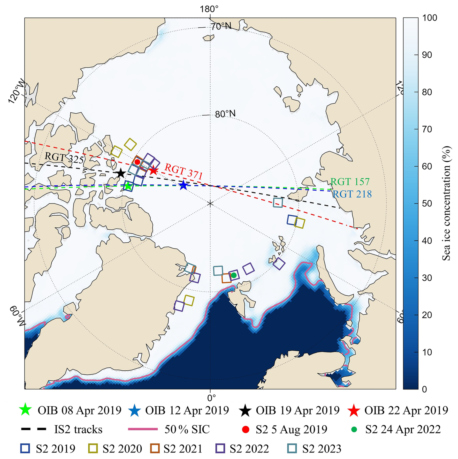
Figure 1 Overview of the study area and multi-source datasets. The background shading shows the mean April monthly SIC during 2019–2023 from the NOAA Climate Data Record (CDR). The magenta contour represents the multi-year mean April 50 % SIC. The dashed lines mark ICESat-2 Reference Ground Tracks (RGT) 157, 218, 325, and 371, with the green, blue, black, and red stars indicating the location of coincident Airborne Topographic Mapper (ATM) measurements. Colored squares denote Sentinel-2 (S2) images from 2019–2023 that spatially coincide with ICESat-2 profiles and were used for training and validation. The red and green dots show the positions of the Sentinel-2 scenes detailed in Sect. 3.2.1.

2.1 ICESat-2 data

ICESat-2 (IS-2) provides a suite of sea ice products derived from its photon-counting lidar observations. The processing workflow begins with geolocated photon clouds (ATL03), progresses to segment-level surface heights and surface-type classifications (ATL07) and along-track freeboard estimates (ATL10), and culminates in gridded monthly freeboard product (ATL20). In this study, HRFM uses ATL03 (Version 6) as the primary input to retrieve surface height, surface type, and freeboard (Sect. 3). ATL07 (Version 6) and ATL20 (Version 5) are used for comparison and evaluation purposes (Sect. 4). Although the newer ATL07 release (Version 7) introduces fixed 10 m segment lengths, it was experimental and limited to strong-beam observations during the study period. Therefore, to ensure a consistent and comprehensive evaluation across both strong and weak beams, ATL07 (Version 6) is used as the comparison reference unless otherwise specified.

2.1.1 ATL03 global geolocated photon data

The ATL03 product provides geolocated and time-tagged photon events detected by ATLAS (Neumann et al., 2023). Each photon is associated with its latitude, longitude, ellipsoidal height, photon-confidence label, background-rate estimates, and geophysical corrections, including corrections for tidal, atmospheric and inverse barometer effects. The photon heights are referenced to the WGS-84 ellipsoid. In HRFM, these corrections are applied to derive the corrected height for each photon.

2.1.2 ATL07 sea-ice height

The ATL07 product provides sea-ice surface heights and surface-type classifications derived from ATL03 photon data for estimating sea-ice freeboard (Kwok et al., 2023). In this product, raw photons are aggregated into adaptive segments containing approximately 150 signal photons, resulting in variable along-track lengths ranging from 10–200 m for strong beams to 40–800 m for weak beams (Kwok et al., 2019b). Surface-height estimation involves a two-stage trimming process: (1) removing photons outside a fixed height window (−2.0 to 3.5 m) and (2) excluding photons beyond two standard deviations of the remaining photons. A dual-Gaussian distribution is then assumed to fit the trimmed histogram to derive the segment's surface height (Kwok et al., 2023).

Surface type is classified using empirical thresholds based on photon rate, background rate, and the width of the photon distribution, informed by Multiple Altimeter Beam Experimental Lidar (MABEL) measurements and post-launch IS-2 assessments (Petty et al., 2021; Kwok et al., 2016). The classified categories include (−1) unknown surface type, (0) cloud covered, (1) non-lead snow/ice surface, (2–5) specular lead, and (6–9) dark lead, denoted by the height_segment_type flag. Specular (dark) lead segments are leads with high (low) photon rates. To mitigate uncertainties in radiometric classification, ATL07 applies a post-classification height filter using neighboring specular lead segments within a 10 km window. A candidate lead's height must lie between the minimum of the specular lead heights (h_{sl_min}) and the larger of (i) the 2nd percentile of specular lead heights, or (ii) h_{sl_min} + 2σ, where σ = 0.02–0.03 m is the expected surface-height uncertainty over specular-lead segments. Segments meeting both classification and height-filter criteria are flagged as ssh_flag = 1, designating them as potential sea surface segments for ATL10 and ATL20 freeboard estimations.

2.1.3 ATL20 gridded sea ice Freeboard

The ATL20 product provides basin-scale Arctic sea-ice freeboard fields as daily and monthly composites on a 25 km × 25 km polar stereographic grid. These gridded fields are derived from along-track ATL10 freeboard estimates using only strong-beam observations (Kwok et al., 2023). To ensure data quality and minimize coastal or open-ocean contamination, ATL20 applies a strict mask, retaining grid cells only where the SIC exceeds 50 % and the distance from the coastline is at least 25 km. In this study, monthly freeboard fields derived from HRFM are compared with the ATL20 from October 2021 to September 2022 to evaluate their basin-scale spatial consistency during the 1-year demonstration period.

2.2 Sentinel-2 data

To construct a robust training dataset for the machine-learning surface-type classifier, we selected Sentinel-2A and -2B scenes near-coincident with IS-2 overpasses during 2019–2023. A maximum time offset of 30 min was applied to minimize misregistration due to sea-ice advection, while retaining a sufficient number of coincident observations. Assuming a typical sea ice drift speed of approximately 0.05–0.1 m s⁻¹, a 30 min offset corresponds to an advective displacement of approximately 90–180 m. This displacement is small relative to the spatial extent of a Sentinel-2 scene, approximately 290 km × 290 km, and can be further reduced by manual alignment based on correspondence between surface optical features and IS-2 photon returns. Because of Sentinel-2's orbital inclination, coincident acquisitions are limited to latitudes south of 82° N.

From an initial pool of 822 overlapping scenes spanning 416 IS-2 tracks, we applied a stringent quality-control procedure. Each scene was manually interpreted using true-color imagery to identify surface types. Leads were distinguished from ice floes based on their characteristic elongated morphology and low reflectance in the visible bands. After extensive manual review, 25 scenes corresponding to 25 IS-2 overpasses were retained as the training and validation dataset. These scenes cover multiple Arctic regions, seasons, sea-ice types, and surface-roughness conditions, with their locations shown in Fig. 1. Their file names, acquisition dates, and time offsets are summarized in Table A1.

2.3 ATM data

The performance of HRFM in retrieving high-resolution along-track heights was evaluated using coincident observations from the Airborne Topographic Mapper (ATM), collected during dedicated IS-2 underflights of NASA's Operation IceBridge (OIB) on April 2019 (Kwok et al., 2019a). The ATM uses a conically scanning green laser lidar (532 nm) that produces footprints approximately 1 m in diameter with a vertical precision of approximately 0.03 m (Krabill et al., 2002). We used ATM profiles from four OIB underflights acquired on 8, 12, 19, and 22 April 2019. These underflights were coincident with IS-2 RGTs 157, 218, 325, and 371, respectively, as shown by the green, blue, black, and red stars in Fig. 1. The four ATM underflights provide independent elevation references for assessing HRFM-derived surface heights and the preservation of fine-scale sea-ice features. Because the degree of spatial overlap and temporal separation differs among the four flights, the ATM comparison statistics are interpreted under the specific collocation described in Sect. 4.1.

3 Method

This section details the implementation of the HRFM for ATL03 photon data. As illustrated in Fig. 2, HRFM consists of two main components. The first component is high-resolution surface-height retrieval, which begins with a two-stage denoising procedure designed to remove background photons and detector after-pulses while preserving morphology-related surface photons as faithfully as possible. The filtered signal photons are subsequently used to estimate surface heights within fixed 5 m along-track segments. The second component is surface-type classification, in which ATL03-derived segment features are interpreted with the aid of coincident Sentinel-2 imagery and used to train a machine-learning classifier. The resulting lead classification provides the local sea-surface reference required for freeboard retrieval.

Figure 2 The flowchart of HRFM.

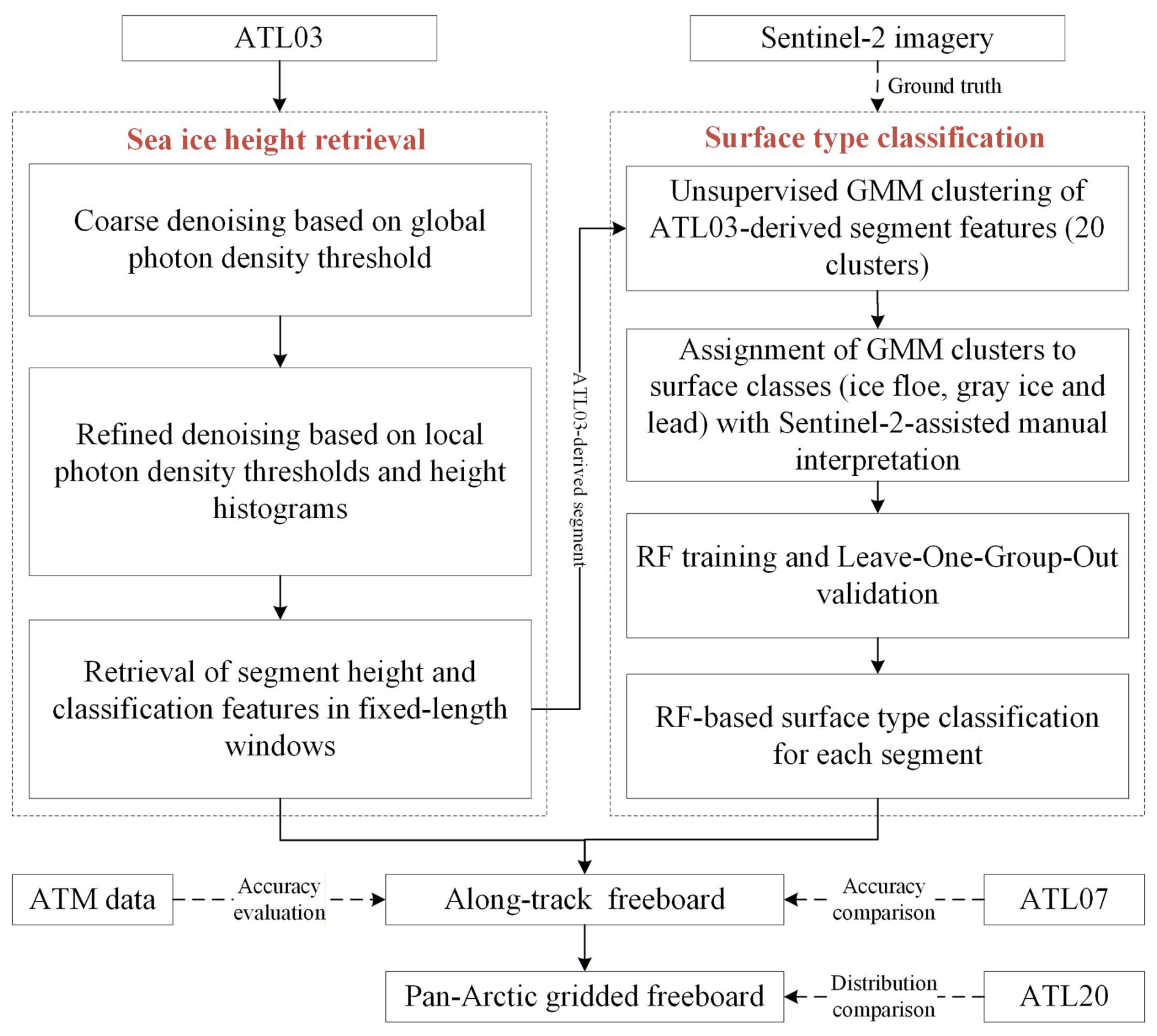
Compared to the ATL07 algorithm, HRFM introduces two main advancements. First, photon-density information is incorporated into both surface-height retrieval and surface-type classification, improving robustness under challenging conditions, such as high solar background, detector saturation, and melt-affected surfaces. This improves the retention of sea ice morphology-related photons, particularly over ridges, narrow leads, and melt ponds, and supports denser surface-height sampling. Second, HRFM uses a machine-learning classifier trained from coincident Sentinel-2 imagery, rather than relying solely on fixed empirical thresholds. This data-driven approach improves the discrimination of sea ice and leads under different seasonal surface conditions, particularly during the melt season when surface radiometric contrast is reduced.

3.1 Surface-height retrieval

As illustrated in Fig. 3a, accurate surface-height retrieval from ATL03 data requires the separation of signal photons (surface) from noise photons (background) originating from solar background, atmospheric scattering, and detector dark counts. HRFM implements a two-stage denoising strategy, consisting of coarse and refined filtering, to extract the final set of signal photons. The resulting signal photon set forms the basis for surface-height retrieval at fixed 5 m segments. The summary of key algorithm parameters used in HRFM is listed in Table A2.

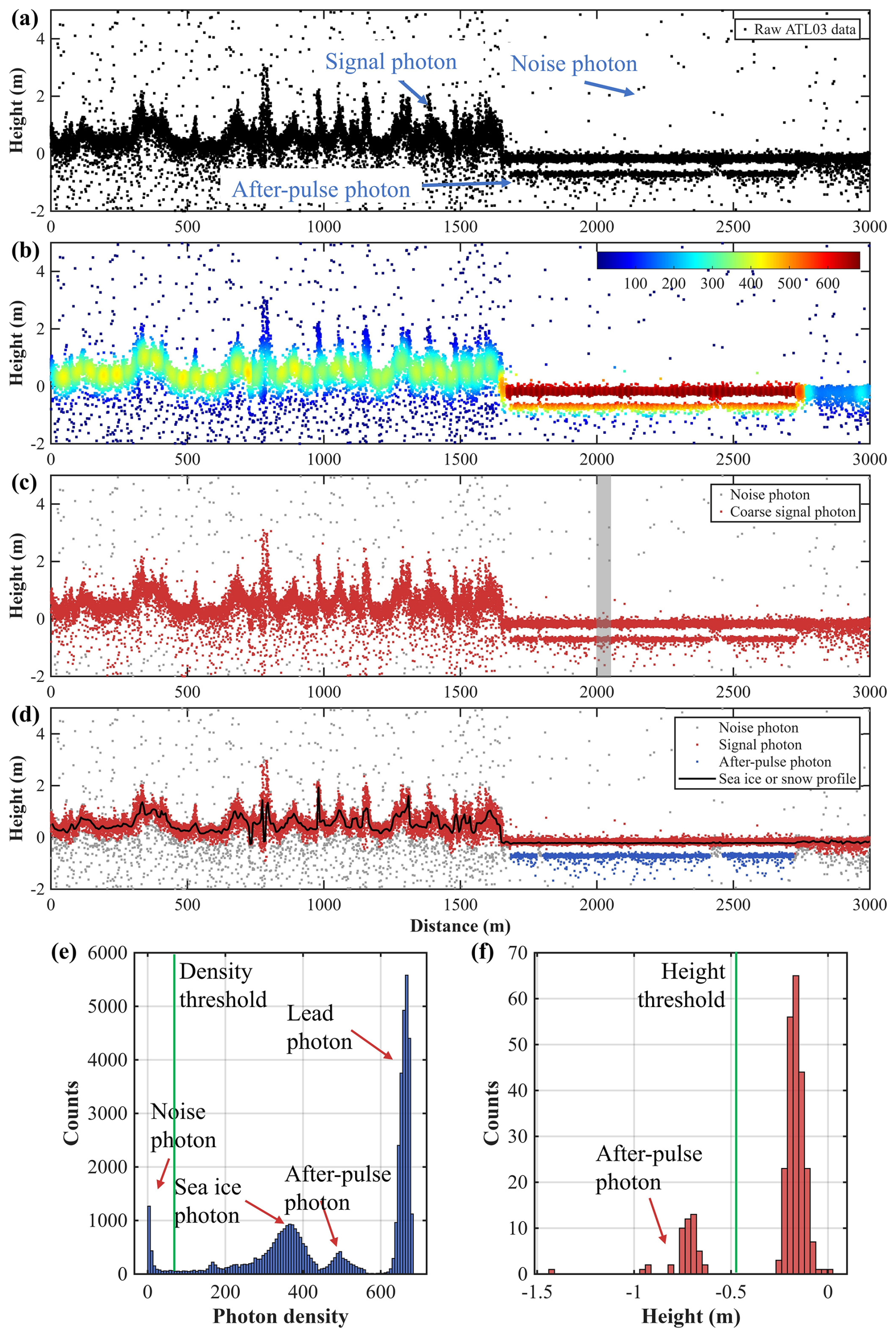
Figure 3 Sequential processing steps for retrieving sea-ice surface height from the middle strong beam of ATL03_20190526002946_08820304_006_02 obtained over the Lincoln Sea. (a) Raw ATL03 data converted into distance-height coordinates. (b) KDE-estimated photon density (the colour bar indicates photon density). (c) Coarse signal photons after density-thresholding and local height-window filtering. (d) Refined signal photons, together with the detected after-pulse photons and the retrieved sea ice or snow surface profile at 5 m along-track resolution. (e) Histogram of photon density corresponding to panel (b). The green vertical line indicates the density threshold used to separate noise photons from coarse signal photon. (f) Height histogram of coarse signal photons within the grey-shaded region in panel (c). The green vertical line denotes the height threshold applied to distinguish after-pulse photons from surface-signal photons.

3.1.1 Coarse denoising

To remove large-scale background noise, raw ATL03 photons are first divided into 3 km along-track segments. Their heights are referenced to the DTU21 Mean Sea Surface (MSS) model (Andersen et al., 2023) to remove geoid trends. Photon density is calculated using a KDE approach. For each photon p, the density D_p is defined as:

$$\begin{array}{}\text{(1)}& D_{\mathrm{p}}=\sum _{i=\mathrm{1}}^{n}K\left(d_{\mathrm{p}i}\right),\end{array}$$

where n is the number of photons within a predefined search region, d_pi is the distance between photon p and neighbor photon i, and K is kernel function (Chu et al., 2017):

$$\begin{array}{}\text{(2)}& K\left(d_{\mathrm{p}i}\right)={\displaystyle \frac{\mathrm{3}}{\mathrm{4}}}\max \left(\mathrm{0},\mathrm{1}-{d_{\mathrm{p}i}}^{\mathrm{2}}\right).\end{array}$$

Since ATL03 photons show much stronger clustering in the horizontal direction than in the vertical direction, distances are computed within an anisotropic elliptical search region:

$$\begin{array}{}\text{(3)}& d_{\mathrm{p}i}=\sqrt{{\displaystyle \frac{\mathrm{\Delta }{x_{\mathrm{p}i}}^{\mathrm{2}}}{a^{\mathrm{2}}}}+{\displaystyle \frac{\mathrm{\Delta }{h_{\mathrm{p}i}}^{\mathrm{2}}}{\mathrm{1}}}},\end{array}$$

where Δx_pi and Δh_pi represent the distances between the two photons in the horizontal and vertical directions, respectively. The horizontal scaling parameter a is set to 25 for strong beams and 100 for weak beams. This process is used to increase the weight of photons in the horizontal direction, thereby preserving the along-track resolution and improving signal-photon extraction (Lu et al., 2025).

Photon densities vary along track due to differences in surface types and beam types (Figs. 3b, A1b, and A2b). To determine a segment-specific threshold that removes noise while retaining morphology-related photons (e.g. ridges or melt ponds), we examine the photon-density distribution within each 3 km segment. The resulting density histogram typically shows a multi-modal structure (Figs. 3e, A1e, and A2e) corresponding to various ground object features: (1) a narrow low-density peak representing noise photons, (2) a broad intermediate-density peak corresponding to sea ice photons, (3) a smaller secondary peak linked to after-pulse photons or weak subsurface scattering, and (4) a high-density peak associated with specular leads.

We fit the noise and sea ice peaks using a two-component Gaussian mixture model (GMM). The intersection of the two fitted components defines the segment-specific density threshold (green lines in Figs. 3e, A1e, and A2e). Photons with densities exceeding this threshold are retained as coarse signal photons (Figs. 3c, A1c, and A2c). The retained coarse signal photons are then further constrained by a local height window, from 2 m below to 6 m above the modal height within each 3 km along-track segment. However, some after-pulse photons and subsurface returns can overlap in density with the sea ice signal; therefore, a second local refinement step is required.

3.1.2 Refined denoising

The retained coarse signal photons are further processed within local 10 m windows to remove residual background photons and detector after-pulses. This refinement step uses different filtering strategies depending on the ATLAS detector saturation state. Saturation is assessed using the signal photon rate, defined as the number of coarse signal photons per transmitted pulse within the local window. Based on ATLAS instrument characterization, detector saturation is identified when the photon rate exceeds 16 photons per pulse for strong beams or 4 photons per pulse for weak beams.

Under saturation conditions, after-pulse echoes can appear at fixed vertical offsets below the true surface, typically approximately 0.45 and 0.9 m (Lu et al., 2021). Because these after-pulse photons can have densities comparable to surface-signal photons, density information alone cannot reliably distinguish these photons. Therefore, a 0.1 m height interval histogram is constructed for each saturated window (Figs. 3f and A1f), and the primary peak is taken as the physical surface. Photons situated more than 0.3 m below this peak are classified as after-pulses and removed, as indicated by the green lines in Figs. 3f and A1f.

For non-saturated windows, remaining noise photons are removed using a locally adaptive density threshold. The threshold is set to the 10th percentile of coarse signal photon densities within the window. Only photons with densities exceeding this threshold are retained as refined signal photons. Together, the coarse and refined denoising stages isolate the final signal photons, as illustrated in Figs. 3d, A1d, and A2d.

We note that the Yet Another Photon Classifier (YAPC) variables provided in recent ATL03 releases offer an additional density-like metric as well, which could be incorporated as an additional filtering variable in future versions of HRFM.

3.1.3 Sea-ice surface-height Estimation

Following refined denoising, surface heights are estimated from the final signal photon set. Although ATL03 provides photon-level observations at an along-track sampling interval of approximately 0.7 m, surface-type classification and freeboard retrieval require statistical estimates at the segment scale. Therefore, the along-track profile is partitioned into fixed 5 m segments after trade-off analyses between spatial resolution and height precision. For each segment, the surface height is defined as the KDE-density-weighted mean of all refined signal photon heights (black lines in Fig. 3d):

$$\begin{array}{}\text{(4)}& H_{\mathrm{seg}}={\displaystyle \frac{{\sum }_{i=\mathrm{1}}^N{D}_i\cdot h_i}{{\sum }_{i=\mathrm{1}}^N{D}_i}},\end{array}$$

where h_i and D_i are the corrected height and KDE-derived density of the ith photon, respectively. Geophysical corrections, including tidal, atmospheric, and mean-sea-surface corrections, as well as the first-photon-bias correction (Kwok et al., 2026) were applied. The corrected segment height relative to the mean sea surface can be summarized as

$$\begin{array}{}\text{(5)}& \begin{array}{rl}{H}_{\mathrm{seg}}=h_{{\mathrm{03}}_{\mathrm{raw}}}& -h_{\mathrm{set}}-h_{\mathrm{sept}}-h_{\mathrm{opt}}-h_{\mathrm{ol}}-h_{\mathrm{mss}}\\ & -h_{\mathrm{ot}}-h_{\mathrm{lpe}}-h_{\mathrm{DAC}}-h_{\mathrm{fpb}}+h_{\mathrm{atm}},\end{array}\end{array}$$

Where $h_{{\mathrm{03}}_{\mathrm{raw}}}$ is the “uncorrected” photon height in ATL03, h_set is the solid earth tide correction, h_sept is the solid earth pole tide correction, h_opt is the ocean loading correction, and h_ol is the ocean pole tide correction, h_mss is the mean sea surface, h_ot is the ocean tide correction, h_lpe is the long period equilibrium tide correction and h_DAC is the dynamic atmospheric correction, h_fpb is the first-photon-bias computed using the system engineering tables supplied in the ATL03, h_atm is the atmospheric path delay range correction. The data source and application of each correction term are summarized in Table A3.

To support the subsequent machine-learning classification, four statistical parameters are extracted for each 5 m segment: (1) photon rate, defined as the number of refined signal photons per transmitted pulse and used as a proxy for relative surface brightness; (2) background rate, defined as the mean ATL03 background rate within the segment and used to represent scattered sunlight at the laser wavelength; (3) height standard deviation (STD), defined as the spread of refined signal photon heights within the segment and used to represent small-scale surface roughness; and (4) mean photon density, defined as the average KDE-derived photon density of the refined signal photons. Following ATL07, the background rate is normalized to a solar elevation angle of 20° (Kwok et al., 2023).

Furthermore, segments impacted by melt ponds are identified by adapting the bimodal height distribution analysis proposed by Herzfeld et al. (2023). A segment is flagged as melt-pond affected when (1) the photon rate remains below the saturation threshold and (2) the height histogram is bimodal, indicating returns from both the pond surface and the pond bottom (Fig. A2). Although such subsurface returns may be useful for potential melt-pond depth retrieval applications (Buckley et al., 2023; Herzfeld et al., 2023), melt-pond-affected segments are excluded from the freeboard estimation to avoid introducing a downward height bias.

3.2 Surface-type classification

Accurate surface-type classification is a prerequisite for reliable freeboard retrieval, as the local reference sea level is determined from identified lead segments. In this section, we first analyze two representative winter and summer scenes using coincident Sentinel-2 imagery to examine the variability of the four HRFM classification parameters across various surface types. We then describe the construction of a labeled training dataset based on unsupervised clustering and visual interpretation. Finally, we introduce the machine learning classifier employed in HRFM to discriminate between floe- and lead-dominated segments.

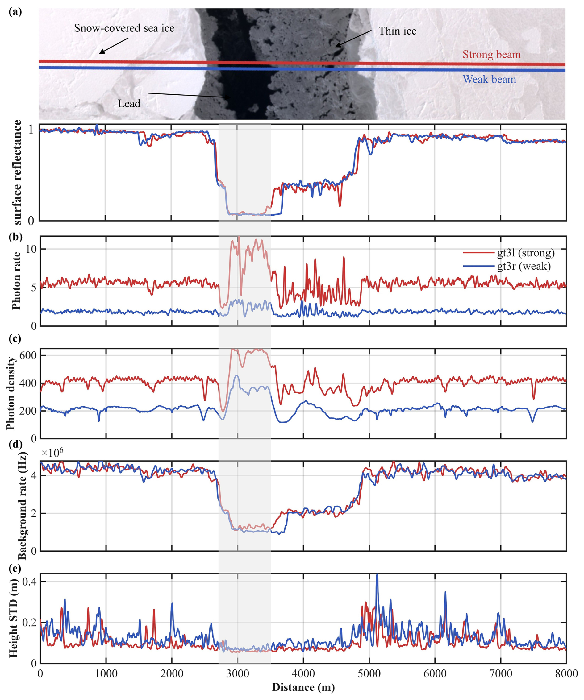
Figure 4 Winter case over an approximately 8 km along-track profile acquired on 24 April 2022. (a) Sentinel-2 RGB imagery (green dot in Fig. 1) overlaid with ICESat-2 gt3l (strong beam, red) and gt3r (weak beam, blue), with surface reflectance derived from the RGB bands of the Sentinel-2 image from nearest neighbor pixels to the ICESat-2 segments. (b) Photon rate, (c) photon density, (d) background rate, and (e) height standard deviation (STD) along track. The gray-shaded region indicates the open-water lead area.

3.2.1 Variability of classification parameters

To characterize the responses of the four HRFM classification parameters across diverse surface types, we analyze two representative IS-2/S-2 coincident scenes: a winter case acquired in April 2022 (Fig. 4) and a summer case affected by melt ponds in August 2019 (Fig. 5). Each scene contains a strong/weak beam pair (gt3l and gt3r) to evaluate beam-dependent sensitivity. Based on the coincident Sentinel-2 imagery, the winter scene suggests visually identifiable snow-covered sea ice, thin young ice with little or no snow cover, and open-water leads (Fig. 4a) whereas the summer scene is characterized by a mixture of open water, melt ponds, bare ice, and residual deteriorated snow (Fig. 5a).

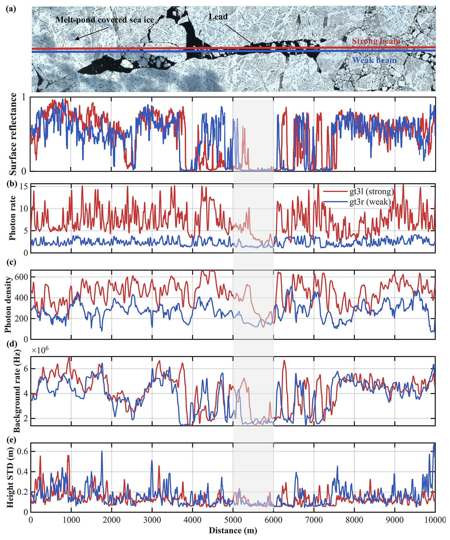
Figure 5 Same as Fig. 4, but for an approximately 10 km along-track profile acquired on 5 August 2019 (red dot in Fig. 1).

In the April (winter) scene, photon rate (Fig. 4b) and photon density (Fig. 4c) generally scale with Sentinel-2-derived surface reflectance over snow-covered and thin ice, yielding relatively stable along-track values. In contrast, pronounced localized spikes are observed over the lead region, where photon rates and photon densities exceed those over adjacent snow-covered ice. These enhancements result from strong specular reflections off smooth open-water or newly formed thin-ice surfaces, which concentrate a large fraction of the emitted laser energy back toward the receiver despite the low reflectance of water (Fig. 4a). However, in the August (summer) scene, specular returns occur with higher frequency due to the widespread presence of melt ponds and narrow leads, resulting in substantially increased along-track variability in both photon rate (Fig. 5b) and photon density (Fig. 5c). Notably, the wide (approximately 1000 m) open-water lead, indicated by the gray shaded region at 5–6 km in Fig. 5, shows simultaneously low photon rate and photon density, unlike the winter case, suggesting a rougher (likely wind-roughened) water surface that scatters energy away from the receiver. This may be related to stronger wind-driven surface waves in summer open water relative to winter conditions (Liu et al., 2016) or the absence of new ice formation in leads compared to the winter case where new ice forms rapidly and truly open water will rarely be present. Across both scenes, weak beams exhibit a reduced dynamic range and diminished contrast, complicating the discrimination between classes. Figure A5 shows the monthly distributions of photon rate and photon density across the annual cycle, further indicating their seasonal difference.

The background rate is predominantly influenced by solar illumination geometry and surface reflection. Its along-track variation closely tracks the intensities in Sentinel-2 RGB imagery and is nearly identical between strong and weak beams (Figs. 4d and 5d), reflecting their shared dependence on solar background. Background rates are highest over bright snow-covered ice (4–5 MHz), intermediate over thin ice (2–3 MHz), and lowest over dark open-water leads (1–2 MHz), qualitatively matching the strong albedo contrast from snow-covered sea ice (0.7–0.8) to open water in leads (0.1–0.2) (Light et al., 2022). In the summer scene, background rate variations increase because melt ponds, bare ice, and wet snow mix over much shorter spatial scales with high spatial heterogeneity in the proportion among components within a single segment.

The height standard deviation reflects local surface roughness and shows a smaller dynamic range than the other parameters (Figs. 4e and 5e). It is higher and more spatially variable over deformed, snow-covered ice, but reduced over thin ice and leads, consistent with their smoother surface conditions.

In summary, while these four parameters provide complementary information for distinguishing sea ice from leads, consistent with early airborne photon-counting lidar studies (Kwok et al., 2016), their responses are highly sensitive to seasonal surface conditions, beam energy, and wind-induced roughness of open water surface, and ice type or age. The resulting nonlinear overlap in feature space motivates the use of a supervised, data-driven classifier for robust surface-type discrimination under both winter and summer conditions.

3.2.2 Training dataset generation

To develop a robust machine-learning surface type classifier, a high-quality labeled dataset was constructed using coincident Sentinel-2 imagery as the ground truth. Given that HRFM generates thousands of 5 m segments per overlapping scene, direct manual annotation of individual segments is impractical. Following the strategy previously developed for improving ATL07 classification (Liu et al., 2025b), we combined unsupervised clustering with visual interpretation to generate the training dataset.

For each coincident IS-2/S-2 scene, HRFM segments were grouped into 20 clusters using a GMM applied to the four classification parameters of photon rate, background rate, height standard deviation, and photon density. This clustering step collapses a large number of segments into a limited number of statistically consistent groups, thereby reducing annotation effort while enhancing labeling robustness. Strong and weak beams were clustered independently because of their different photon statistics.

Since the unsupervised clustering itself does not reveal surface type, each cluster was assigned a label using Sentinel-2 RGB imagery. Following the same visual interpretation criteria and alignment method for Sentinel-2 and IS-2 as in our earlier ATL07 work (Liu et al., 2025b), the clusters were manually assigned to three surface types: sea ice, thin ice, and leads.

Figure 6 illustrates the mean values and standard deviations of the classification parameters for clusters derived from a representative strong-beam data on 24 April 2022. The clusters align with the expected parameter behaviors summarized in Sect. 3.2.1, indicating that they map consistently onto physical surface types. Sea ice clusters are characterized by high background photon rates and larger height standard deviations. Thin-ice clusters exhibit intermediate photon rates, photon densities, and background rates, with moderate height variability. Lead clusters are distinguished by either very high photon rates and densities associated with specular returns or very low photon rates and densities associated with dark leads, together with low background rates and small height standard deviations.

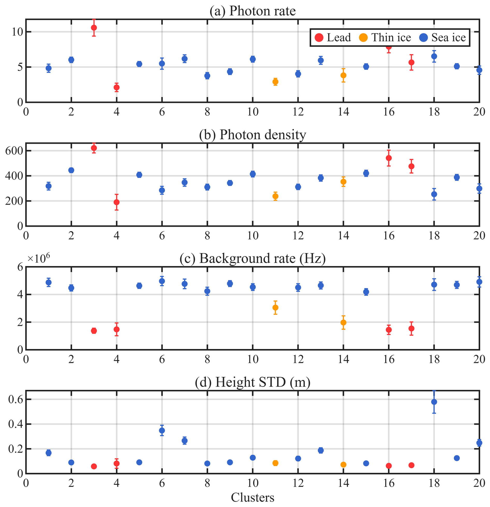
Figure 6 Mean values and standard deviations of the four classification parameters for clusters derived from ICESat-2 observations on 24 April 2022 (the winter case). Panels show (a) photon rate, (b) photon density, (c) background rate, and (d) height standard deviation (STD). The surface types are color-coded as lead (red), thin ice (yellow), and sea ice (blue).

For freeboard retrieval, misclassifying non-lead surfaces as lead segments is more problematic than the opposite case, because false lead detections can bias the local sea-surface reference and subsequently propagate into the freeboard estimates. Therefore, clusters were assigned to the lead class only when they appeared as clearly dark, open-water-like features in Sentinel-2 imagery and were consistent with the local ATL03 photon characteristics. Ambiguous surfaces were not labelled as leads unless they could be confidently interpreted as open-water leads.

Several transitional surface types remain difficult to separate using the available optical information. Therefore, the thin-ice class is used as a broad category that includes visually similar transitional ice types, such as nilas, frazil ice, and slush ice. In addition, melt-pond-covered ice clusters was conservatively treated as sea ice class, even when the ponds appeared dark in Sentinel-2 imagery. This choice was made to avoid misclassifying melt ponds as leads and incorrectly using them as sea-surface reference points in the freeboard retrieval. It should be noted that the manual labeling inevitably introduces some subjectivity and classification uncertainty, especially for transitional or ambiguous surface types.

This labeling process was applied consistently to 25 coincident IS-2/S-2 scenes shown in Fig. 1, representing a wide distribution across the Arctic and a multi-year temporal range from 2019 to 2023. The final aggregated dataset comprises 1 029 289 labeled strong-beam segments and 1 023 895 labeled weak-beam segments, providing a substantial and diverse foundation for training the machine-learning classifier.

3.2.3 Training of machine learning classifier

With the labeled training dataset established, a supervised Random Forest (RF) classifier is employed to assign surface types to each HRFM segment. Consisting of an ensemble of decision trees, the RF algorithm is well-suited for this application due to its ability to capture complex, non-linear relationships among physical parameters without requiring feature normalization (Breiman, 2001). RF is computationally efficient and has been widely adopted in studies on sea ice classification (Fredensborg Hansen et al., 2021; Mugunthan et al., 2023; Shen et al., 2017). Furthermore, the ensemble-averaging nature of RF could mitigate sensitivity to mislabeling within the training data, which is unavoidable when surface labels are derived from Sentinel-2-assisted visual interpretation of statistically aggregated clusters.

The RF classifier was configured with 200 decision trees and a maximum tree depth of 20 to ensure a balance between model complexity and computational efficiency. Separate models were trained for strong and weak beams to account for their distinct signal-to-noise ratios and dynamic ranges. The classification relies on the four primary features: photon rate, background rate, height standard deviation, and mean photon density. Previous studies indicated that photon rate and mean photon density provide the highest discriminative power for detecting specular leads, while background rate is crucial for separating thin ice from snow-covered ice (Koo et al., 2023; Kwok et al., 2016; Liu et al., 2025b).

To ensure robust generalization across diverse spatial and seasonal conditions, we implemented a Leave-One-Group-Out (LOGO) cross-validation strategy. In each iteration, data from one entire coincident IS-2/Sentinel-2 pass was held out for testing, while the remaining 24 scenes were used for training. This approach prevents spatial autocorrelation from overinflating accuracy estimates and ensures the model can handle unseen geographical regions.

The trained classifier assigns a surface type of sea ice, thin ice, or lead to every HRFM segment. Segments previously identified as melt-pond influenced (details in Sect. 3.1.3) are excluded prior to classification to avoid ambiguity during the melt season.

Two classification settings were evaluated. First, a three-class classifier was trained to distinguish sea ice, thin ice, and lead, allowing the separability of transitional ice types to be assessed. Second, for the final freeboard retrieval, a conservative binary classifier was used in which thin ice was merged into the sea-ice class. This binary setting reduces the risk of using uncertain thin-ice segments as lead segments for local sea-surface reference construction. After the LOGO evaluation, the final binary RF classifiers for strong and weak beams were trained using all 25 labeled scenes and applied to the full HRFM dataset.

3.3 Sea-ice freeboard estimation

Following surface-height retrieval and surface-type classification, HRFM derives freeboard at two spatial scales: along-track freeboard and monthly gridded freeboard fields.

(1) Along-track freeboard calculation

The along-track freeboard is computed by subtracting a local sea-surface reference from the heights of identified sea-ice segments. As the optimization of the local sea-surface reference is not the primary focus of this study, a pragmatic and efficient approach is adopted. Specifically, all lead segments identified within each 10 km along-track window are aggregated to estimate the local sea-surface height. To reduce the influence of spurious lead detections, lead heights falling outside three standard deviations of the window mean are excluded. The mean height of the remaining lead samples is then used as the local sea-surface reference for that window. In 10 km windows without valid lead detections, the local sea-surface reference is estimated by linear interpolation between the neighboring 10 km windows to ensure continuity.

(2) Gridded monthly freeboard

To generate composite maps of the Arctic freeboard and facilitate direct comparison with the ATL20 product, monthly gridded freeboard fields are generated on a 25 km polar stereographic grid (EPSG:3411). All valid along-track freeboard observations acquired within a given month are projected onto this grid. For each grid cell, the freeboard value is computed as a distance-weighted average of all contributing observations. Grid cells with no valid observations during the month are left empty.

4 Results

4.1 Surface-height evaluation and comparison

To quantitatively evaluate the surface-height retrieval performance of HRFM and compare it with ATL07, we used coincident ATM observations within approximately 10 km along-track segments. ATM and ICESat-2 profiles were directly collocated without applying the cross-correlation maximization procedure used by Kwok et al. (2019a). Before comparison, HRFM, ATL07, and ATM heights were all referenced to the DTU21 mean sea surface to ensure a consistent reference. For each HRFM or ATL07 segment, the raw ATM heights falling within the corresponding along-track segment extent and an approximately 11 m footprint were averaged to obtain the reference ATM height. The averaged ATM heights associated with ATL07 segments were subsequently resampled to the HRFM segment spacing to facilitate a consistent comparison and to illustrate the resolution differences between the two products.

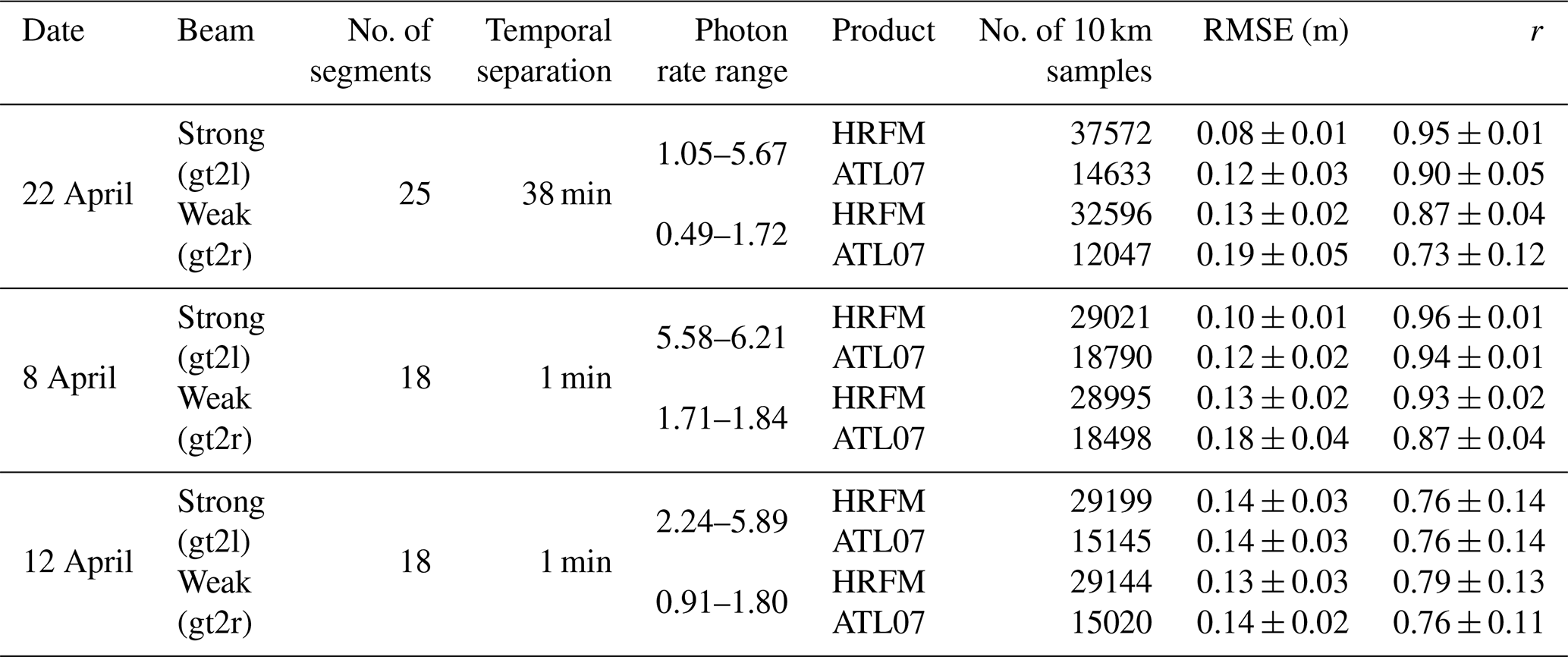
Among the four ATM underflights acquired on 8, 12, 19, and 22 April 2019, the 22 April case provides the clearest overlap with both the strong and weak ICESat-2 beams and is therefore used for the main validation shown in Fig. 7. Additional checks for the 8 and 12 April underflights are provided in Figs. A3 and A4, respectively. The 19 April underflight was examined but was not used for quantitative statistics because the spatial overlap with the corresponding ICESat-2 ground track was insufficient for a reliable segment-wise comparison. A summary of the observational conditions and validation results for all underflights is provided in Table 1. Because no along-track shifting was applied in this study, the reported RMSE and correlation values should be interpreted as a relative comparison between HRFM and ATL07 under the same non-shifted collocation framework, rather than as a strict replication of the optimized ATM–ICESat-2 validation procedure of Kwok et al. (2019a).

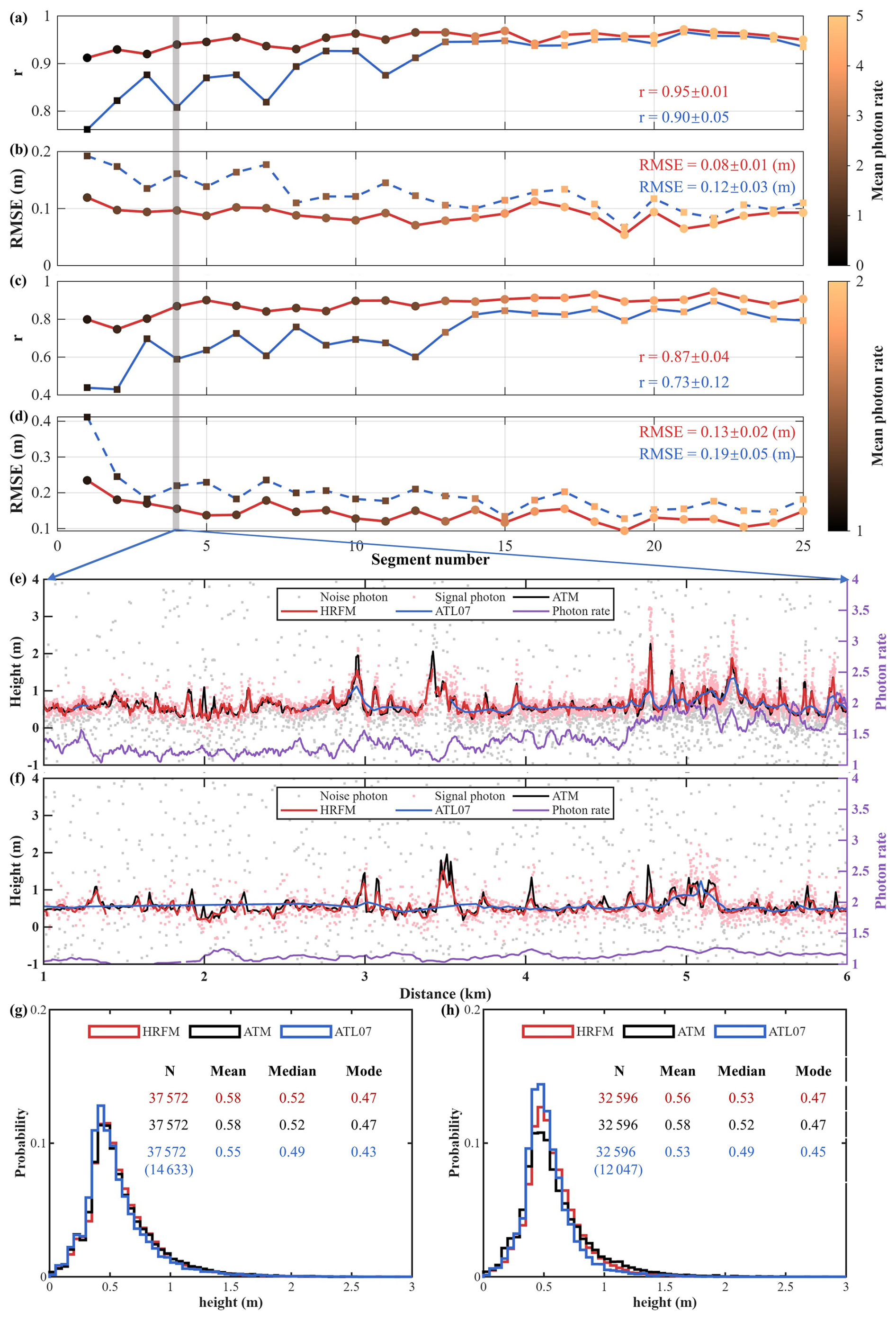
Figure 7 Evaluation of HRFM and ATL07 surface-height retrievals against ATM observations obtained on 22 April 2019. The comparison was performed using direct, non-shifted collocation, with HRFM, ATL07, and ATM heights referenced to the DTU21 mean sea surface. (a, b) Correlation coefficient (r) and root-mean-square error (RMSE) between ATM and ICESat-2 surface heights from HRFM (red) and ATL07 (blue) for the strong beam. (c, d) Same as (a, b), but for the weak beam. The color scale indicates the mean photon rate for each segment. (e, f) Surface-height profiles of segment 4 for strong and weak beams, respectively, including ATM heights (black), HRFM heights (red), ATL07 heights (blue), HRFM-identified signal (pink) and noise (gray) photons, and the corresponding photon rate (purple). (g, h) Distributions of surface-height estimate for all 25 segments for strong and weak beams, respectively, with the number of observations (N), mean, median, and mode indicated for each dataset. Numbers in parentheses denote the original number of ATL07 samples before resampling.

Figure 7a and b summarize the correlation coefficient (r) and root-mean-square error (RMSE) between ATM observations and IS-2 surface heights retrieved by HRFM and ATL07 for the strong beam (gt2l) and weak beam (gt2r), respectively, on 22 April 2019. The 25 along-track 10 km segments are ordered according to their mean photon rate. For both beams, HRFM shows higher correlations with ATM, with r = 0.95 ± 0.01 for the strong beam and r = 0.87 ± 0.04 for the weak beam, compared with r = 0.90 ± 0.05 and r = 0.73 ± 0.12 for ATL07, respectively. HRFM also achieves lower RMSE values of 0.08 ± 0.01 and 0.13 ± 0.02 m for the strong and weak beams, respectively, compared with 0.12 ± 0.03 and 0.19 ± 0.05 m for ATL07. The improvement is most evident in the lower-photon-rate segments, particularly segments 1–14, suggesting that the HRFM retrieval strategy improves surface-height retrieval under low-photon-rate conditions, particularly for the weak beam.

Table 1 Summary of the comparison between HRFM and ATL07 against ATM observations for all underflights.

The along-track profiles for a representative case (segment 4) are shown in Fig. 7e and f for the strong and weak beams, respectively. HRFM closely follows the ATM profile and captures height variability associated with ice ridges. In contrast, ATL07 produces smoother profiles and does not fully resolve some ridge peaks when the photon rate is low. This is consistent with the different algorithm designs. Under low-photon-rate conditions, ATL07 tends to use longer segments, which can smooth fine-scale surface-height variability and increase the likelihood of spanning mixed surface types, whereas HRFM retains a fixed 5 m sampling scale. Figure 7g and h present the distributions of surface-height estimates from HRFM, ATL07, and ATM aggregated over all 25 segments. The aggregated distributions further show that HRFM is closer to ATM in terms of the mean, median, and mode. In comparison, the ATL07 distributions are shifted towards lower heights, with mean, median, and mode values approximately 0.02–0.04 m lower than those of ATM, consistent with previous studies (Duncan and Farrell, 2022; Kwok et al., 2019a; Ricker et al., 2023). As indicated by the sample counts shown in parentheses, HRFM retains more valid surface-height samples than ATL07 across the examined segments. By refining the signal photon extraction and operating at a fixed 5 m along-track scale, HRFM preserves a larger fraction of observations associated with individual ridges and provides a denser representation of sea-ice surface topography.

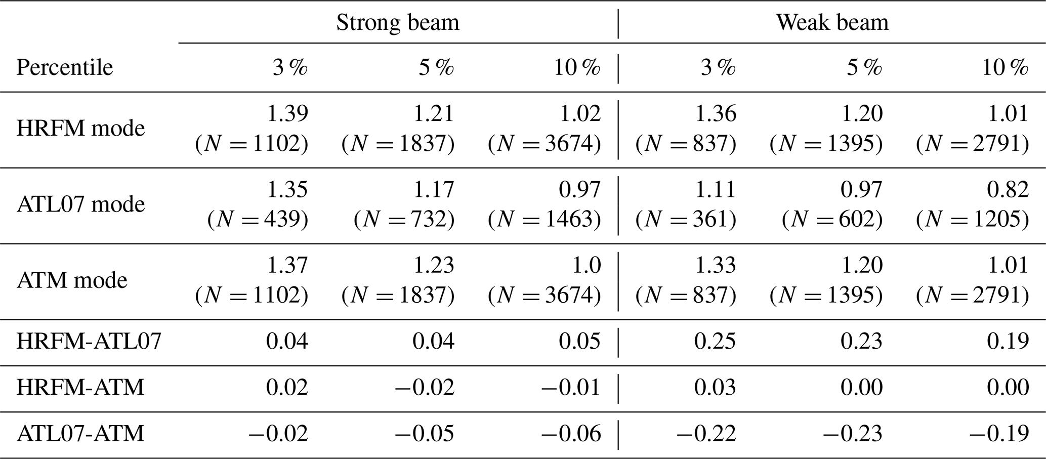
Table 2 summarizes the modal values of the upper 3 %, 5 %, and 10 % of the surface-height distributions for HRFM, ATL07, and ATM for both strong and weak beams, together with their pairwise differences. The differences between HRFM and ATM modes remain small (−0.02 to +0.03 m) and show no dependence on percentile or beam type. ATL07 modes are lower than the corresponding ATM modes in all cases. This difference is particularly large for the weak beam, reaching −0.19 to −0.23 m at the 3 %–10 % levels. These results further indicate that the stronger smoothing in ATL07 can reduce the representation of ridge-related surface-height extremes, with potential implications for estimates of sea-ice surface roughness and associated processes such as atmospheric form drag, wind stress, and ice–structure interactions (e.g., Krumpen et al., 2025; Mchedlishvili et al., 2023; Muilwijk et al., 2024).

Table 2 Modal surface-height values (m) derived from the upper 3 %, 5 %, and 10 % of the height distributions for HRFM, ATL07, and ATM from strong and weak beams on 22 April 2019. Values in parentheses indicate the number of valid observations (N).

While the ATM comparison provides a quantitative validation of HRFM surface-height retrieval over thick, consolidated ice, the available ATM observations are mainly located north of Greenland, where the sea-ice surface is relatively rough and open-water leads are infrequent. To further assess the impact of signal photon extraction on surface-height estimation under flat-surface conditions, we examine two cases with open-water lead cases using ICESat-2 observations and coincident Sentinel-2 imagery.

Figure 8 illustrates the signal-photon extraction and surface-height retrieval over two visually identifiable open-water leads, as confirmed by the coincident Sentinel-2 imagery in Fig. 8a and d. In the photon-profile panels (Fig. 8b and e), HRFM distinguishes between noise (gray), signal (pink), and after-pulse (orange) photons, producing relatively stable surface-height estimates (red lines) over the selected lead regions. By contrast, the ATL07 signal-selection envelope (green dashed lines) incorporates a broader range of lower-height photons in these cases, including photons associated with subsurface scattering and detector after-pulses. This leads to physically inconsistent height fluctuations in the ATL07 profile (blue lines).

Because open-water leads are expected to have relatively flat surfaces, the downward excursions in the ATL07 profiles are more likely related to the inclusion of non-surface photons than to true surface topography. The height distributions in Fig. 8c and f further illustrate this difference. HRFM produces narrow, approximately unimodal height distributions, whereas ATL07 shows broader and, in these examples, partly bimodal distributions. The lower ATL07 modes are located approximately 0.05–0.10 m below the HRFM peak, and the mean ATL07 lead heights are 0.03–0.04 m lower than the corresponding HRFM estimates.

These examples indicate that after-pulse photons can affect lead height estimation when they are identified as signal photon. If such lead segments are used to construct the local sea-surface reference, the lowered lead-height estimate would propagate into the freeboard retrieval and could lead to a positive freeboard bias of approximately 0.03–0.04 m in these cases. This highlights the importance of robust photon filtering and after-pulse treatment for high-resolution freeboard retrieval.

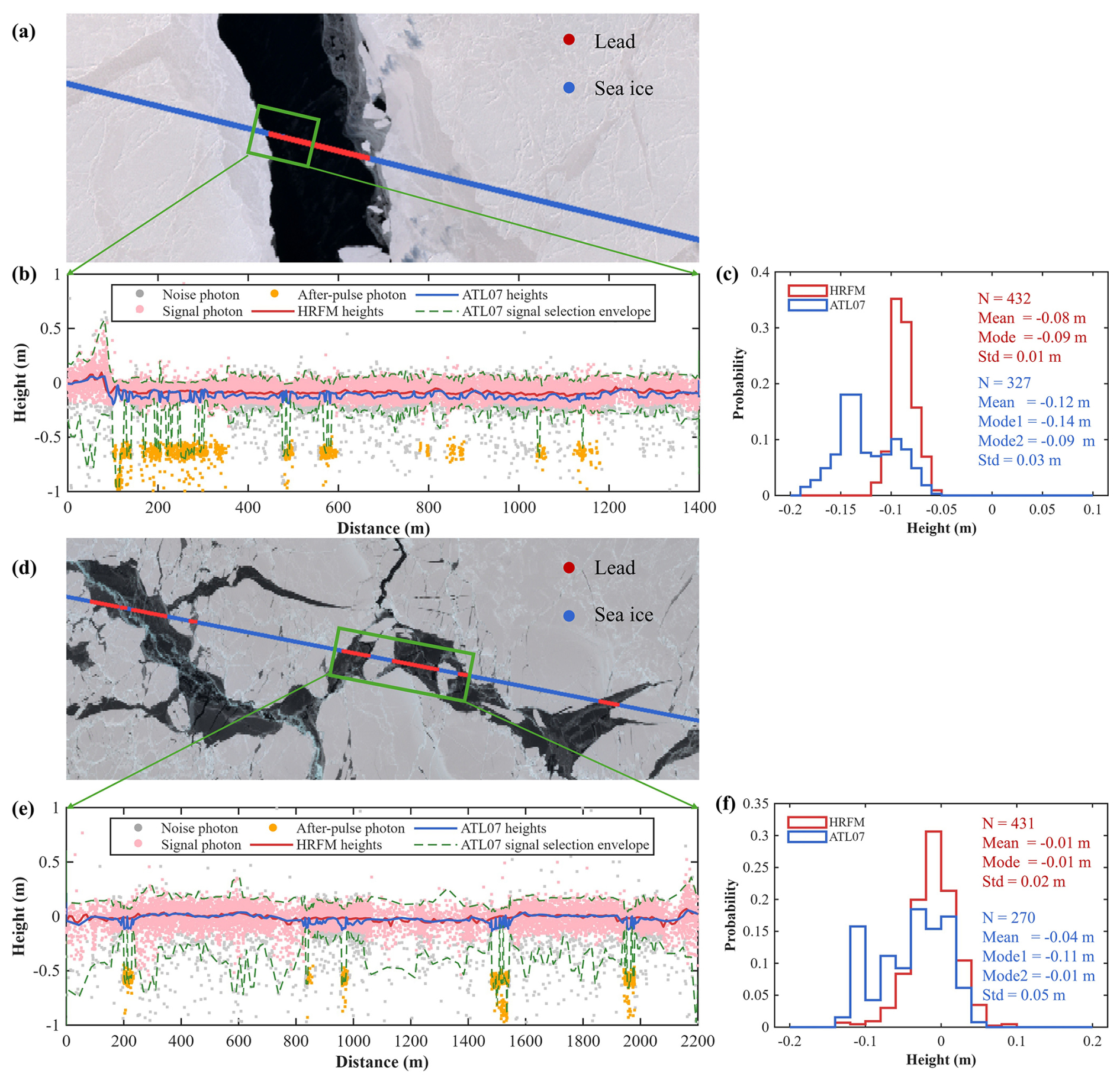
Figure 8 Surface-height retrieval over open-water leads and comparison between HRFM and ATL07 for ATL03_20220424135203_04961504_006 and ATL03_20220510145813_07411505_006. (a, d) Coincident Sentinel-2 imagery showing the ICESat-2 ground tracks and HRFM surface-type classification. Red and blue points indicate lead and sea-ice segments, respectively, and the green boxes mark the enlarged regions shown in the photon-profile panels. (b, e) Along-track ATL03 photon clouds and surface-height retrievals within the selected lead regions. Gray, pink, and orange points denote background, signal, and after-pulse photons identified by HRFM, respectively. The green dashed lines represent the ATL07 signal-selection envelope. The red lines show HRFM surface heights, while the blue lines represent ATL07 surface heights. (c, f) Probability distributions of surface-height estimates derived from HRFM (red) and ATL07 (blue) within the selected lead regions.

4.2 Surface-type classification validation and comparison

Figure 9 provides a qualitative validation of HRFM surface-type classification using coincident Sentinel-2 imagery as an independent visual reference, together with a direct comparison against ATL07 across a range of observation conditions. For ATL07, two surface-type flags are considered: height_segment_type and ssh_flag, as described in Sect. 2.1.2.

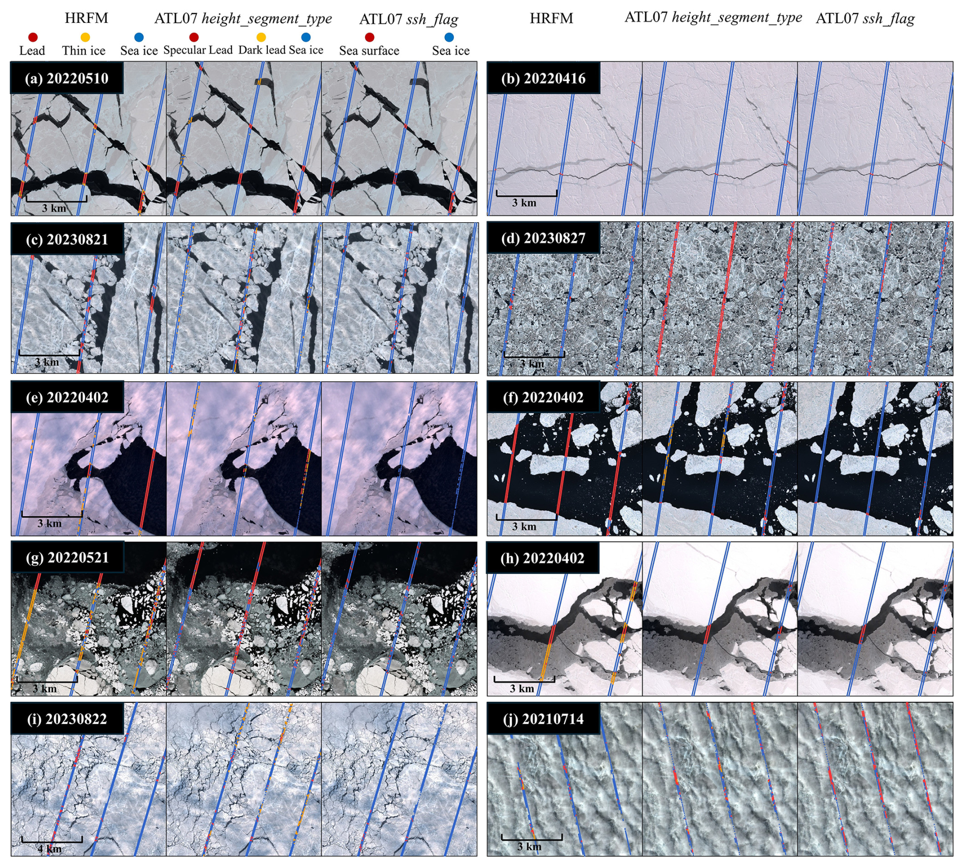
Figure 9 Comparison of surface-type classification from HRFM and ATL07 for (a, b) winter cases, (c, d) summer melt-season cases, (e, f) large-lead cases, (g–h) thin-ice cases, (i, j) cloud -affected cases. Coincident Sentinel-2 optical images acquired within 30 min of the ICESat-2 overpasses are shown as background images and used as an independent visual reference for evaluating the classifications. The HRFM classification results are from Leave-One-Group-Out (LOGO) tests. The ICESat-2 footprint size is not to scale.

Under favorable winter conditions (Fig. 9a and b), the HRFM and ATL07 classifications are generally consistent with the Sentinel-2 imagery for both strong and weak beams. Both methods detect major leads at the kilometer scale and narrow cracks smaller than approximately 50 m. The agreement between strong and weak beams in these cases indicates that classification is less limited by beam energy under high-contrast winter surface conditions.

The differences between HRFM and ATL07 become more evident under challenging surface conditions. During the summer melt season (Fig. 9c and d), widespread melt ponds increase photon rates (Fig. 5b) and photon densities (Fig. 5c), reducing the contrast between open water and melt-pond-covered ice. The fixed-threshold algorithm used in ATL07, originally tuned for winter conditions, associates high photon rates with open water and therefore misclassifies segments of melt-pond-covered ice as leads. If such segments are used in local sea-surface reference construction, elevated ice or melt-pond surface heights may be included in the reference surface, which can introduce a negative bias in the retrieved freeboard. In these cases, HRFM more consistently distinguishes true open-water leads from melt-pond-covered ice, producing surface-type classifications that agree more closely with Sentinel-2 imagery.

Figure 9e and f illustrate additional differences related to large dark leads. Large leads with low albedo and wind-roughened surfaces often exhibit reduced specular returns and lower photon rates and photon densities (Fig. 5). Under these conditions, ATL07 may classify portions of open water as dark leads or sea ice. As dark-lead segments are not used as sea-surface segments in ATL07, their exclusion reduces the number of valid open-water samples available for local sea-surface reference estimation. This can increase the uncertainty of the reference sea level and subsequently affect freeboard retrieval. In contrast, HRFM identifies these visually apparent open-water regions as leads more consistently, particularly where specular returns are sparse.

Beyond lead detection, Fig. 9g and h show that HRFM can distinguish thin ice as a separate surface class in winter cases. ATL07 separates open water into specular and dark lead categories, but it does not explicitly distinguish thin ice from thicker snow-covered sea ice; most thin-ice surfaces are therefore included in the general sea-ice category. HRFM provides a finer partitioning of surface types by separating thin ice from both open water and thicker sea ice. This distinction is useful for surface-type interpretation and process studies, because thin ice is associated with enhanced conductive heat flux through the ice and stronger turbulent exchange above the surface compared with thicker ice (Uhlíková et al., 2024). However, for the final freeboard retrieval, thin ice is conservatively merged with sea ice in the binary classifier, as described below, to avoid using uncertain thin-ice segments as lead segments.

Finally, Fig. 9i and j illustrate the impact of cloud-affected conditions on surface-type classification. Under optically thin clouds (Fig. 9i), ATL07 occasionally misclassifies portions of sea ice as dark leads, as reported by Kwok et al. (2021). Under optically thick clouds (Fig. 9j), cloud scattering can weaken the effective surface return, reduce photon rates, and distort classification features, leading to missing observations or misclassification in both HRFM and ATL07. To reduce the influence of such cases in subsequent freeboard retrieval, HRFM lead segments with fewer than 10 valid signal photons and a height standard deviation greater than 0.8 m are excluded from local sea-surface reference construction.

Table 3 summarizes the LOGO cross-validation results for the HRFM three-class surface-type classifier. Statistics are reported separately for strong and weak beams, including overall accuracy, precision, and recall values. Here, precision value quantifies false positives, defined as the fraction of correctly classified segments among all segments assigned to a class, whereas recall value quantifies false negatives, defined as the fraction of correctly classified segments among all reference segments of that class.

For both beam types, HRFM achieves high overall accuracy, with 0.98 for strong beams and 0.97 for weak beams. For strong beams, sea ice is classified with a precision of 0.99 and a recall of 0.99, while lead detection reaches a precision of 0.96 and a recall of 0.95. For weak beams, sea-ice classification, with a precision of 0.98 and a recall of 0.99, whereas lead performance is slightly reduced, with a precision of 0.94 and a recall of 0.91. This reduction is consistent with weaker photon statistics and lower signal-to-noise ratios that can blur the separation between open water and low-reflectance ice surfaces.

Table 3 Confusion matrices and classification accuracy statistics for the HRFM three-class surface-type classifier based on leave-one-group-out (LOGO) cross-validation over tracks with a total length of approximately 10 000 km.

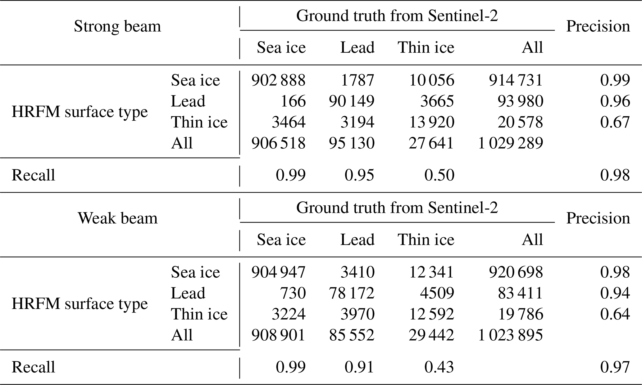
Classification uncertainty is larger for thin ice. The precision and recall for thin ice are 0.67 and 0.50 for strong beams and decrease to 0.64 and 0.43 for weak beams. This is expected because thin ice represents a transitional surface state: its photon rate, background rate, height standard deviation and photon density often fall between those of snow-covered ice and leads, leading to overlapping feature distributions and increased confusion. In addition, thin-ice labeling from Sentinel-2 imagery is intrinsically less certain than the identification of open water or bright snow-covered ice, which propagates into the reference labels and limits achievable class separability.

To isolate the classification performance most directly affecting freeboard retrieval, we also evaluated a two-class setting in which thin ice is merged into sea-ice class. Overall accuracy increases to 0.99 for strong beams and 0.99 for weak beams (Table A4), indicating that most errors in the three-class problem arise from ambiguity within ice subclasses rather than from confusion between sea ice and leads. Therefore, the final full-year HRFM freeboard retrieval uses the binary RF classifier with only two classes, sea ice and lead. This conservative setting reduces the risk of using uncertain thin-ice segments as lead segments for local sea-surface reference estimation.

After this independent evaluation, the final binary RF classifier was trained using all 25 labelled scenes and applied to the full-year HRFM data.

4.3 Year-round sea-ice freeboard

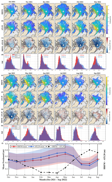
The gridded freeboard estimates from HRFM and the official ATL20 product from October 2021 to September 2022 are compared in Fig. 10. The within-grid-cell standard deviations of the monthly HRFM freeboards are shown in Fig. A6. To facilitate comparison with ATL20, which is generated from strong-beam ATL10 freeboards, this gridded comparison uses HRFM retrievals from the central strong beam. During this one-year demonstration period, HRFM provides monthly freeboard estimates over most of the Arctic Ocean and shows broader spatial coverage than ATL20 in several months. Both products display broadly consistent Arctic-wide spatial distribution patterns (Fig. 10a–b, e–f), with larger freeboards generally found north of Greenland and the Canadian Arctic Archipelago. These regions are associated with older sea ice and thicker snow cover. The histograms of gridded freeboard (Fig. 10d and h) further illustrate the statistical consistency between the two products.

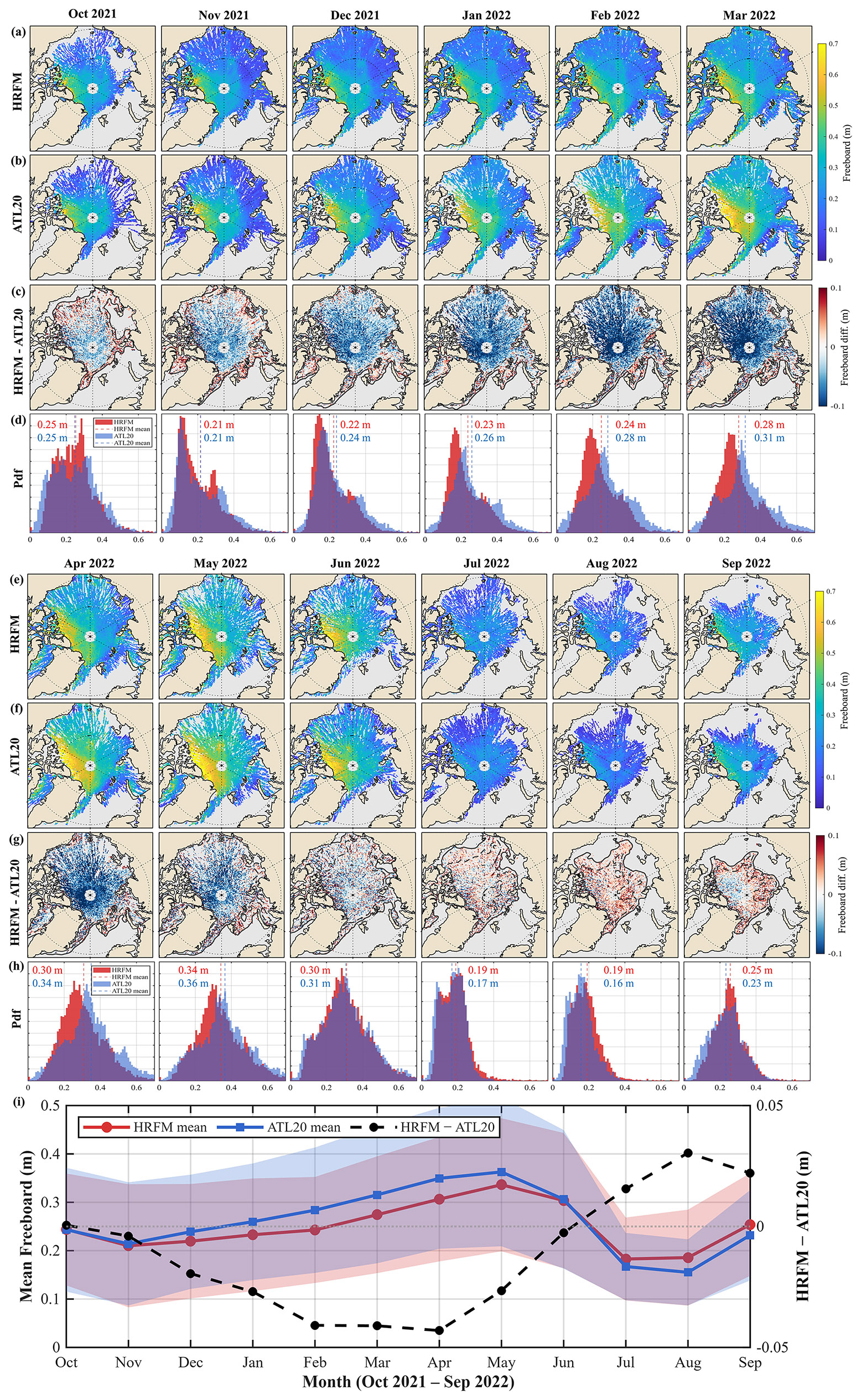
Figure 10 Monthly gridded sea-ice freeboard from October 2021 to September 2022. (a, e) Monthly mean freeboard estimated using HRFM. (b, f) Corresponding monthly mean freeboard from the ATL20 product. (c, g) Spatial differences between the two products (HRFM − ATL20). (d, h) Histograms of gridded freeboard for HRFM (red) and ATL20 (blue), with dashed vertical lines indicating the respective monthly means. (i) Time series of monthly mean freeboards from HRFM (red) and ATL20 (blue), with shaded areas representing ±1 standard deviation around the monthly mean. The dashed black line indicates the monthly mean difference between HRFM and ATL20.

The spatial distribution of freeboard differences (HRFM − ATL20) reveals two distinct patterns related to zones of SIC (Fig. 10c and g). Positive differences are mainly observed in low-SIC regions (< 90 %), whereas negative differences dominate in high-SIC areas (> 90 %). large and dynamically evolving leads are more frequent, and the local sea-surface reference can be difficult to estimate robustly. Ocean–ice interactions, waves, and swell within expansive leads may introduce additional height variability (Bateson et al., 2020), so a limited set of detected lead samples may not fully represent the local sea-surface height. In this context, gridded freeboard differences between HRFM and ATL20 may partly reflect the different lead-detection strategies used in the two products. HRFM identifies a larger population of visually apparent lead segments, whereas the ATL07 processing chain uses a more conservative set of sea-surface segments. Conversely, in compact high-SIC areas dominated by thick ice, leads are sparse. As noted by Petty et al. (2021), there are fewer specular leads available from the ATL07 product in these regions compared to more seasonal ice regions, which can lead to the freeboard difference between the ATL07-based ATL20 product and our HRFM.

The monthly evolution of basin-averaged freeboard during this 1-year demonstration period is shown in Fig. 10i. HRFM yields lower mean freeboard than ATL20 from October to May, whereas it yields slightly higher mean freeboard during much of the melt season from June to September. These monthly differences likely arise from the combined effects of factors related to surface-height retrieval, lead detection, local sea-level reference construction, and gridding. During winter, narrow and smooth leads are more susceptible to ATLAS detector saturation, which can generate after-pulse photons below the true water surface (Fig. 8). HRFM explicitly identifies and removes such after-pulse returns, whereas residual noise photons may still be included in the ATL07 signal-selection envelope in some cases. This can lower the estimated lead height and consequently increase ATL20 freeboard when such leads are used for sea-surface reference construction. In addition, the more conservative ATL07 sea-surface flag identifies a smaller subset of available leads, whereas HRFM detects a larger number of lead segments. This difference may affect the representativeness of the local sea-surface reference.

During the melt season, melt-pond-covered ice becomes more prevalent, increasing the likelihood that pond-covered ice surfaces are confused with open-water leads in threshold-based classification (Fig. 9c, d). If such segments are used as sea-surface reference points, the reference surface may be biased upward, leading to lower freeboard estimates. HRFM reduces this risk by using a machine-learning classifier trained with Sentinel-2-assisted labels and by conservatively excluding melt-pond-affected segments from lead-based sea-surface reference construction. These differences in lead identification and surface-height filtering provide a plausible explanation for the monthly HRFM–ATL20 differences observed during the one-year demonstration period. The combined effects of improved surface-height retrieval and surface-type classification on along-track freeboard estimation are further examined in Sect. 5.2.

Although HRFM demonstrates improved performance in along-track surface-height retrieval and surface-type classification relative to ATL07, systematic differences remain between gridded HRFM freeboards and the ATL20 product. It should be noted that differences in reference sea-level construction and gridding methods may also contribute to the observed discrepancies at the grid scale. The observed differences provide a valuable insight into how surface-height retrieval and lead detection strategies influence basin-scale freeboard estimates.

5 Discussion

5.1 Inter-beam consistency and weak-beam performance

IS-2 uses a multibeam configuration consisting of three strong-weak beam pairs. The weak beams transmit approximately 25 % of the energy of the strong beams and have therefore been used less extensively in sea-ice studies because of their lower signal-to-noise ratios. One objective of this study is to evaluate whether HRFM can provide stable freeboard retrievals from weak-beam observations and thereby increase effective sampling density and spatial coverage. In addition, previous studies have reported inter-beam range biases in IS-2 observations, including centimeter-level differences among strong beams in Arctic sea-surface height anomaly retrievals (Bagnardi et al., 2021) and ice-sheet elevation measurements (Brunt et al., 2021), with persistent biases associated with strong beam 1. Such inter-beam inconsistencies raise concerns about the joint use of six beams for freeboard estimation.

To evaluate inter-beam consistency and weak-beam performance in freeboard retrieval, we calculated the monthly mean freeboards using six different beams respectively (Fig. 11). The monthly mean freeboards derived from the six beams show generally consistent temporal variations throughout the 1-year demonstration period. During the freezing season from October to May, differences among the six beams are mostly below 0.01 m (Fig. 11a). During the summer melt months, however, slightly larger inter-beam differences appear, particularly between the middle beam pair and the outer beam pairs. The maximum monthly deviation reaches approximately 0.02 m. This difference may be related to the increased complexity of surface conditions, lower transmitted energy level (∼ 80 % of outer beams, Kwok et al., 2019b) and decreased valid observations due to clouds compared to winter.

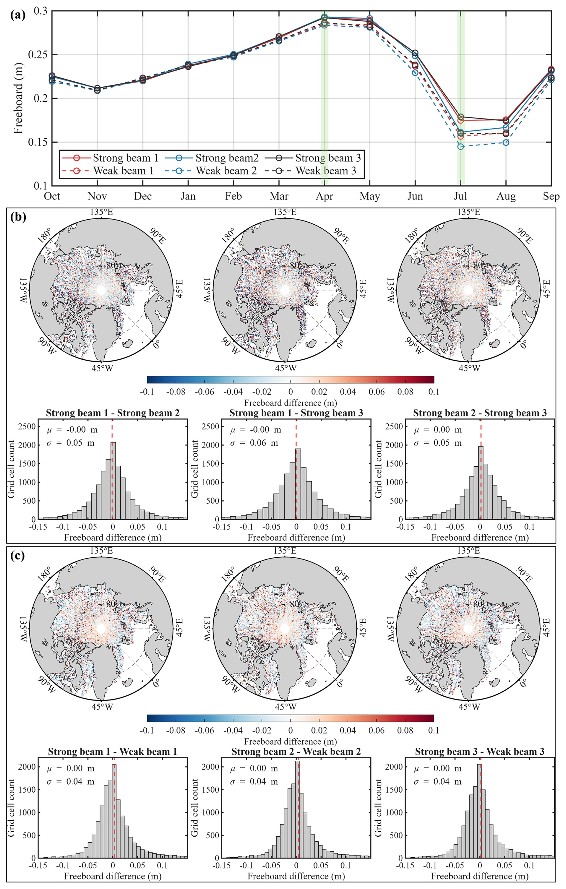
Figure 11 Inter-beam comparison of HRFM freeboard retrievals. (a) Monthly mean freeboard from October 2021 to September 2022 for the three strong beams (solid lines) and the corresponding weak beams (dashed lines). The green vertical bands highlight April and July, which are used for the spatial inter-beam comparisons. (b) Spatial distribution of gridded freeboard differences among strong beams for April 2020 (Strong beam 1 − Strong beam 2, Strong beam 1 − Strong beam 3, and Strong beam 2 − Strong beam 3). The corresponding histograms show the mean (µ) and standard deviation (σ) of each difference distribution. (c) Same as (b), but for differences between corresponding strong–weak beam pairs (Strong beam 1 − Weak beam 1, Strong beam 2 − Weak beam 2, and Strong beam 3 − Weak beam 3).

Figures 11b and A7a show the spatial distributions and histograms of freeboard differences among the three strong beams for April and July 2022, respectively. Figures 11c and A7b show the corresponding differences between each strong–weak beam pair. In April, the differences among strong beams and between corresponding strong–weak beam pairs show no clear regional pattern across the Arctic basin. Their histograms are centered near zero, with mean differences close to 0.00 m and standard deviations of approximately 0.04–0.06 m. In July, the differences remain broadly centered near zero but show slightly larger beam-dependent offsets. In particular, the middle beam shows a mean offset of approximately −0.01 to −0.02 m relative to the outer beams, and weak beams show a small negative offset relative to their corresponding strong beams.

The limited impact of inter-beam range bias on HRFM freeboard estimates is likely related to the differential nature of freeboard retrieval. Freeboard is derived as the relative height between the ice surface and a locally determined sea-surface reference along the same beam. Therefore, beam-dependent absolute range offsets can be partly cancelled when both ice-surface heights and lead-based sea-surface references are retrieved within the same beam. By stabilizing surface-height retrieval and lead identification under low-photon conditions, HRFM further reduces the sensitivity of weak-beam retrievals to their lower transmitted energy. As a result, weak-beam freeboards are broadly consistent with strong-beam freeboards at the monthly gridded scale, although small centimetre-level inter-beam differences remain, especially during the melt season.

These results indicate that weak-beam observations can provide useful additional information for HRFM freeboard retrieval. Weak-beam freeboards not only achieve accuracy comparable to strong beams but also generate spatially coherent freeboard maps independently. This enhanced inter-beam consistency implies that future IS-2 sea ice freeboard and thickness products could benefit from jointly exploiting all six ATLAS beams. In the present HRFM framework, this means combining freeboard estimates that are independently retrieved for each beam, thereby increasing effective sampling density, improving spatial coverage, and reducing gridded uncertainty, particularly in regions and seasons where observations are otherwise sparse (Ricker et al., 2023). A related but distinct approach is to construct a swath-like sea-surface reference to retrieve sea-ice freeboard by using sea-surface points across beams, which has also been explored in ATL07/ATL10 algorithm development (Kwok et al., 2026).

5.2 Potential sources of freeboard difference

The monthly contrasting freeboard differences between HRFM and ATL20 may partly arise from differences in surface-height estimation, surface-type classification, and local sea-surface reference construction. Two examples (from winter and summer conditions) in Fig. 12 present how to determine the local sea level reference using the surface height and surface type from HRFM and ATL07 (including height_segment_type and ssh_flag). The reference sea level is the mean height of lead segments for HRFM, specular lead segments for ATL07 height_segment_type and sea surface segments for ATL07 ssh_flag. Above the reference level (blue line) is the freeboard of the floating ice cover.

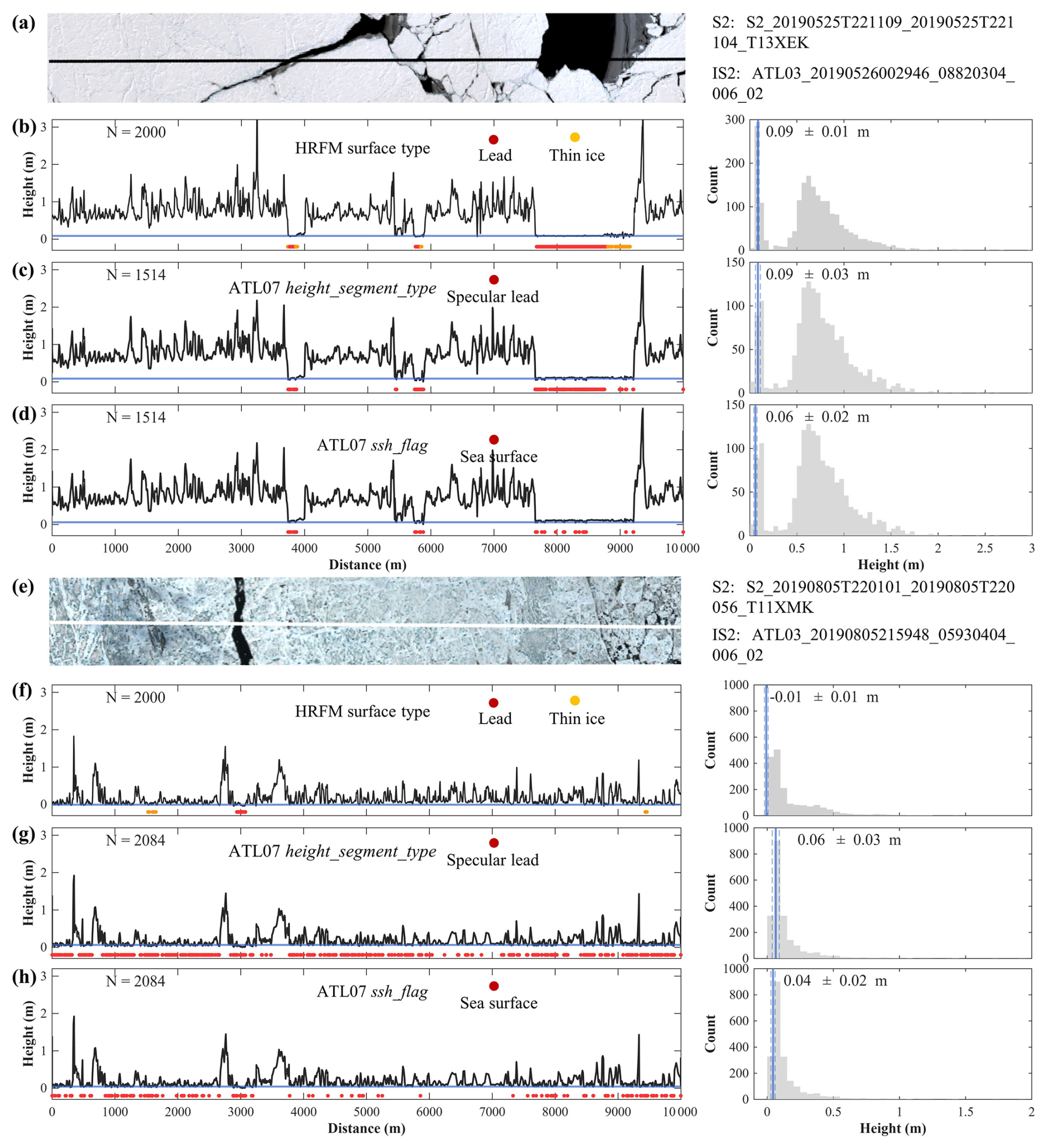
Figure 12 Determination of the local sea-surface reference in 10 km segments using surface heights and surface-type classifications from HRFM and ATL07. Two examples are shown for (a–d) 26 May 2019 and (e–h) 5 August 2019. (a, e) Coincident sentinel-2 imagery with IS-2 tracks shown in black and white. Surface heights and surface-type classifications from (b, f) HRFM, (c, g) ATL07 height_segment_type, and (d, h) ATL07 ssh_flag are used to estimate the local sea-surface references (blue lines), respectively. N is the number of height segments within each 10 km example. Quantity on right panel shows the calculated local sea-surface reference (mean and standard deviation).

For the winter example, HRFM provides surface-type classifications that are more consistent with Sentinel-2 imagery than those from ATL07, together with a more stable surface-height retrieval over lead regions (Fig. 12b). As shown by the height distributions on the right-hand side of Fig. 12, the HRFM-derived reference sea level is 0.09 ± 0.01 m, indicating that the retained lead segments form a compact and internally consistent sea-surface sample. When the ATL07 height_segment_type classification is used, the reference sea level is close to 0.09 m, but exhibits a larger standard deviation (0.03 m). This larger standard deviation reflects the inclusion of lead segments whose surface heights are locally underestimated, partly due to residual after-pulse photons that are not fully removed in the ATL07 processing chain, as illustrated in Fig. 8. The ATL07 ssh_flag represents an additional height-based filtering applied to the height_segment_type surface types (Sect. 2.1.2). This filtering preferentially retains lower-height specular lead segments, while discarding a large fraction of valid lead segments (Fig. 12c and d). Consequently, the number of retained sea-surface samples is markedly reduced, and the resulting reference sea level decreases to 0.06 ± 0.02 m, which is lower than both the HRFM- and height_segment_type–based estimates. This downward shift in the reference sea level explains why ATL07-based freeboard estimates (ATL20) tend to be higher than HRFM during winter conditions.

Under summer melt conditions, the dominant source of differences shifts from height filtering to surface-type misclassification. Extensive melt ponds reduce the contrast of classification features and cause ATL07 height_segment_type to misclassify large fractions of melt-pond-affected sea ice as leads (Fig. 12g). Consequently, the reference sea level derived from height_segment_type is elevated to 0.06 ± 0.03 m, compared to the HRFM reference sea level of about −0.01 ± 0.01 m. Although the ssh_flag filtering removes some high-height segments and lowers the reference sea level to 0.04 ± 0.02 m (Fig. 12h), a number of misclassified sea ice segments remain. These residual errors continue to bias the ATL07-based reference sea level upward relative to HRFM, leading to systematically lower freeboard estimates in summer.

The plots in Fig. 13 best show the difference of reference sea level determination between HRFM and ATL07 during winter and summer examples. Figure 13a and b show the relevant statistics from fifty 10 km segments in the 26 May 2019 and 05 August 2019 tracks, respectively. HRFM estimates are generally higher than ATL07 in winter but lower in summer. Crucially, HRFM exhibits a smaller standard deviation in identified lead heights compared to ATL07, suggesting that HRFM achieves lower uncertainty by effectively filtering outliers in the lead detection process. It is noteworthy that during the summer melt season, the height range of lead segments expands for all methods due to the challenging surface-type classification.

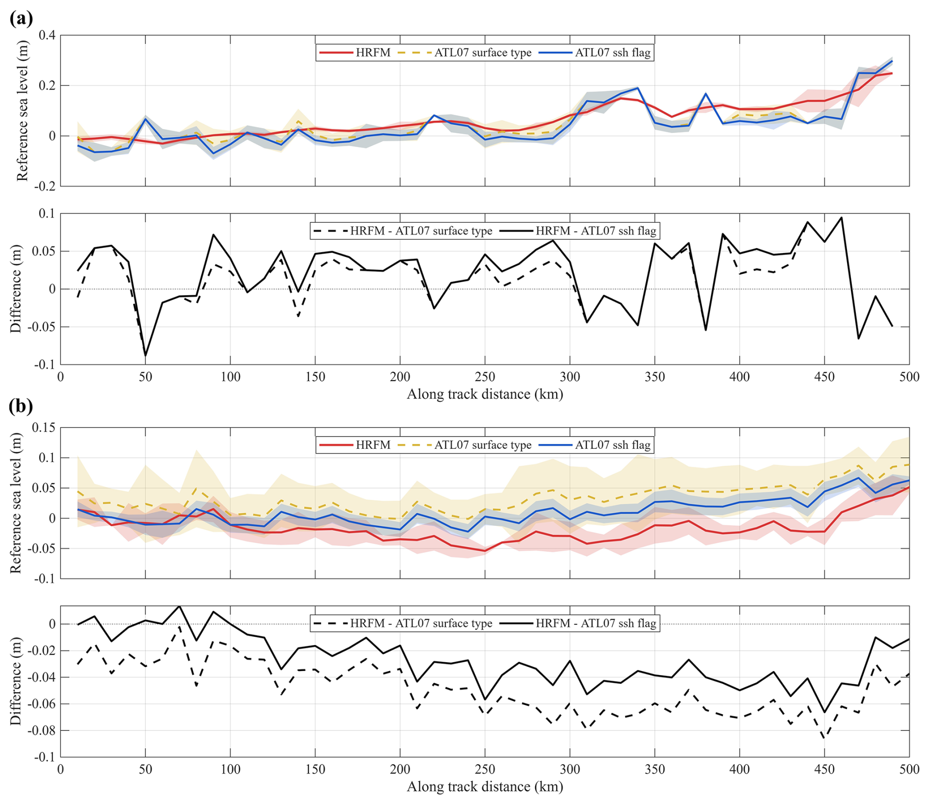
Figure 13 Determination of local sea-surface references along fifty consecutive 10 km segments for ICESat-2 ground tracks acquired on (a) 26 May 2019 and (b) 5 August 2019. The upper panels show the local sea-surface references derived from HRFM (red solid line), ATL07 surface_type (yellow dashed line), and ATL07 ssh_flag (blue solid line), with shaded envelopes indicating ±1 standard deviation of the selected lead or sea-surface heights within each 10 km segment. The lower panels present the corresponding differences between HRFM and the two ATL07-based reference estimates.

Taken together, these differences in reference sea-level estimation might lead to the observed seasonal reversal in HRFM–ATL20 freeboard differences: HRFM freeboards are generally lower than ATL20 during winter, when ATL07 filtering removes many valid lead samples, but higher during summer, when melt-pond-affected ice is erroneously included in the reference sea-surface estimate. Similar winter–summer contrasts have been reported by Koo et al. (2023) in Antarctic sea ice freeboard, and are also consistent with recent findings by Petty et al. (2025), who showed that IS-2–derived sea ice thickness tends to be higher than CryoSat-2 estimates, with lower winter freeboards yielding improved inter-sensor consistency.

5.3 Possible limitations and future work

Despite the improved performance of HRFM in along-track surface-height retrieval, surface-type classification, and inter-beam consistency, several limitations remain and should be considered when interpreting the results of this study.

First, independent validation of gridded freeboard estimates at basin scale remains limited. Comparisons with ATM profiles provide useful validation of surface-height retrieval over thick, consolidated ice, but comparable independent observations are scarce for summer conditions and for large spatial scales (Saylam et al., 2025). Consequently, the absolute accuracy of gridded HRFM freeboards cannot yet be conclusively quantified. Future efforts combining airborne campaigns, autonomous platforms, and coordinated satellite observations will be essential for evaluating grid-scale freeboard products, particularly during the melt season.

Second, HRFM relies on a supervised machine-learning classifier trained using coincident optical imagery. While the leave-one-group-out cross-validation results indicate good performance across the tested beam types, surface conditions, and seasons, generalization to a broader range of atmospheric and illumination conditions remains an important consideration. Background photon rates are strongly affected by solar illumination and can become very low under low solar-elevation conditions. Under such conditions, classification uncertainty may increase because one of the key discriminative features becomes less informative. Following established ATL07 practices (Kwok et al., 2016, 2023), the background rate was excluded as a classification feature when the solar elevation angle was below 15°. Future work could address this limitation by incorporating a larger and more diverse training dataset and by exploring classification models that exploit along-track contextual information from multiple adjacent segments, rather than relying solely on features derived from individual signal segments. Such approaches may help reconcile robustness under low background conditions with improved separability of surface types, thereby further strengthening year-round surface-type classification and freeboard retrieval.

Third, although HRFM includes photon-density filtering, local height-window constraints, and after-pulse treatment, challenging atmospheric or pointing-related conditions can still affect photon retrieval and surface-type classification. In particular, cloud-attenuated returns, low signal strength, and potential pointing issues may reduce the reliability of individual segments. Future HRFM dataset construction will therefore benefit from incorporating additional ATL03 quality-control information, such as PODPPD-related flags and beam-angle information, to identify and flag potentially affected observations more systematically.

6 Conclusions

In this study, we developed and implemented the High-Resolution Freeboard Method (HRFM), a novel processing framework designed to retrieve high-resolution sea-ice freeboard directly from ICESat-2 ATL03 photon data. By improving signal photon extraction, surface-height retrieval, and surface-type classification, HRFM addresses several challenges in photon-counting laser altimetry over sea ice, including signal denoising in complex environments, detector after-pulse contamination, weak-beam underutilization, and melt-pond-related classification ambiguity.

HRFM employs a two-stage denoising strategy to extract signal photons associated with fine-scale ice morphology, including ridges, leads, and melt ponds, allowing along-track surface heights to be resolved at 5 m intervals. Validation against airborne ATM data demonstrates that HRFM achieves lower RMSE and higher correlation than ATL07 under the same non-shifted collocation framework. For the strong beam, HRFM reduces the RMSE from 0.12 ± 0.03 m for ATL07 to 0.08 ± 0.01 m and increases the correlation from 0.90 ± 0.05 to 0.95 ± 0.01. HRFM also better preserves small-scale ridge-related height variations and reduces lead-height fluctuations associated with lower-elevation after-pulse-contaminated photons.

Melt ponds remain a major obstacle for year-round freeboard retrieval as they reduce the contrast between sea ice and open-water leads. HRFM addresses this issue using a machine-learning surface-type classifier trained with 25 coincident Sentinel-2/ICESat-2 scenes, comprising more than 2 million labeled 5 m segments. The three-class classifier distinguishes sea ice, thin ice, and leads, while the final freeboard retrieval uses a conservative binary classifier in which thin ice is merged into the sea-ice class. This design reduces the risk of using uncertain thin-ice or melt-pond-affected segments as lead segments for local sea-surface reference construction. In the independent LOGO evaluation, the binary classifier achieves an overall accuracy of 0.99 for both strong and weak beams, supporting robust lead detection for freeboard retrieval.

Comparative analysis with the ATL20 product shows that while HRFM freeboard maps maintain consistent large-scale spatial patterns, they exhibit monthly mean differences of up to ±0.04 m. HRFM yields lower freeboard estimates in winter by retaining more valid lead samples and removing after-pulse photons, but produces higher freeboard estimates in summer by effectively excluding misclassified melt ponds in the determination of reference sea level.

An additional contribution of HRFM is the enhanced performance of weak beams, which yield freeboard estimates statistically consistent with those from strong beams. This capability might enable the joint utilization of all six ICESat-2 beams, increasing the actual area of sensed sea ice and reducing uncertainties in gridded freeboard products. Our ongoing work aims to extend HRFM to long-term ICESat-2 observations to construct continuous, cross-season records of sea ice freeboard and thickness, providing a high-fidelity dataset for sea ice forecasting and climate change investigations in the Arctic.

Appendix A

Table A1 Summary of the 25 Sentinel-2/ICESat-2 coincident scenes used for training and validation.

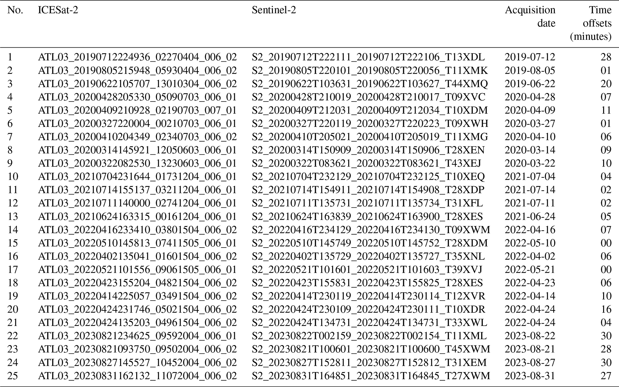
Table A2 Summary of key algorithm parameters used for HRFM photon denoising, surface-height retrieval, surface-type classification, and freeboard estimation.

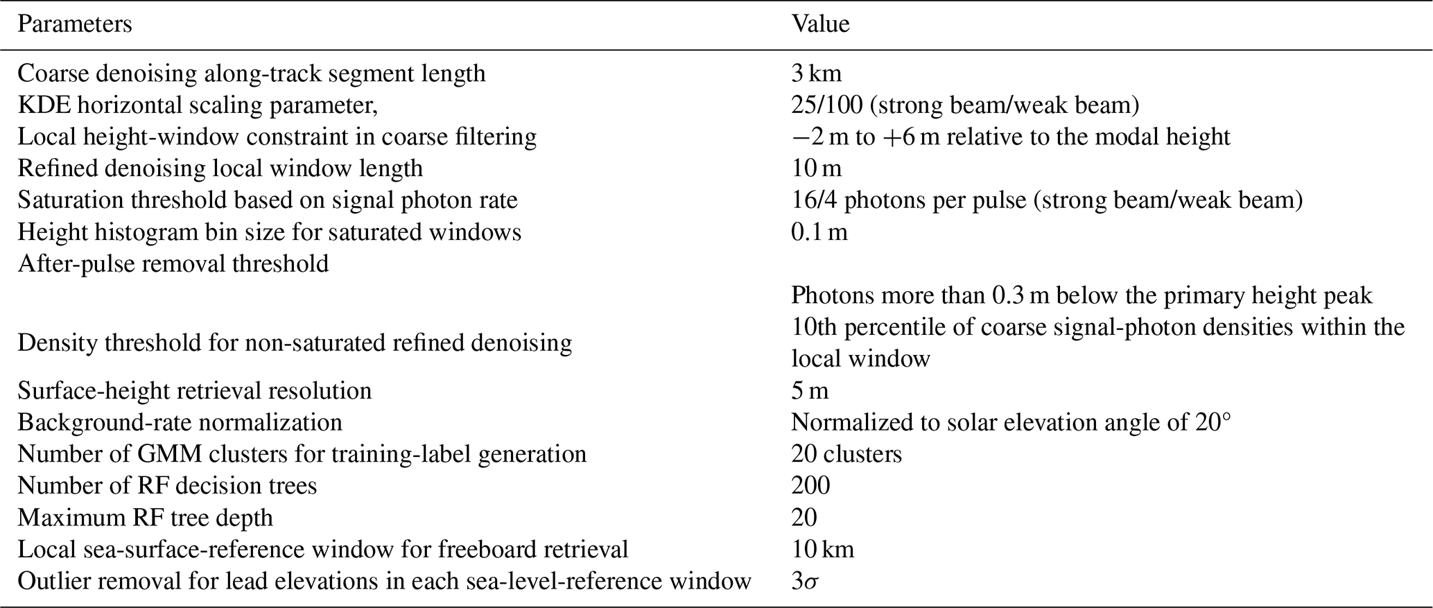
Table A3 Summary of correction terms and mean sea-surface models used in HRFM and ATL07.

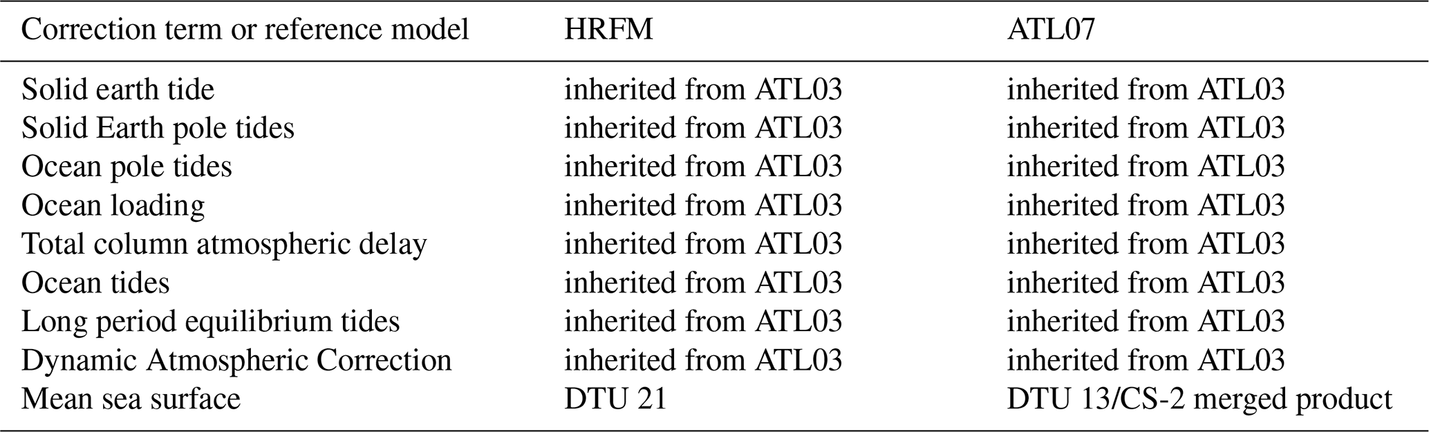
Table A4 Confusion matrices and classification accuracy statistics for the HRFM surface-type classifier based on leave-one-group-out (LOGO) cross-validation, when thin-ice type is merged into sea-ice type

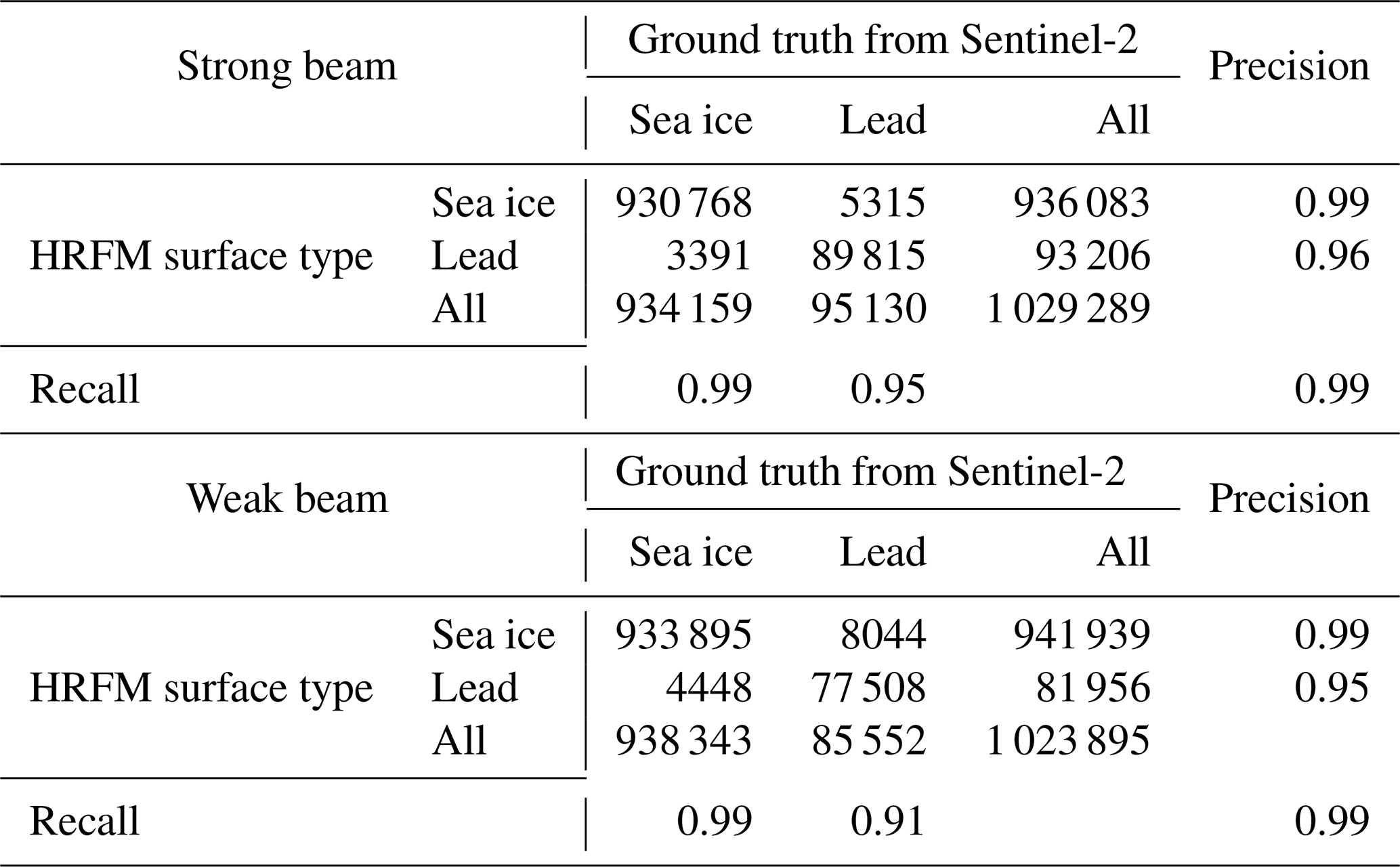
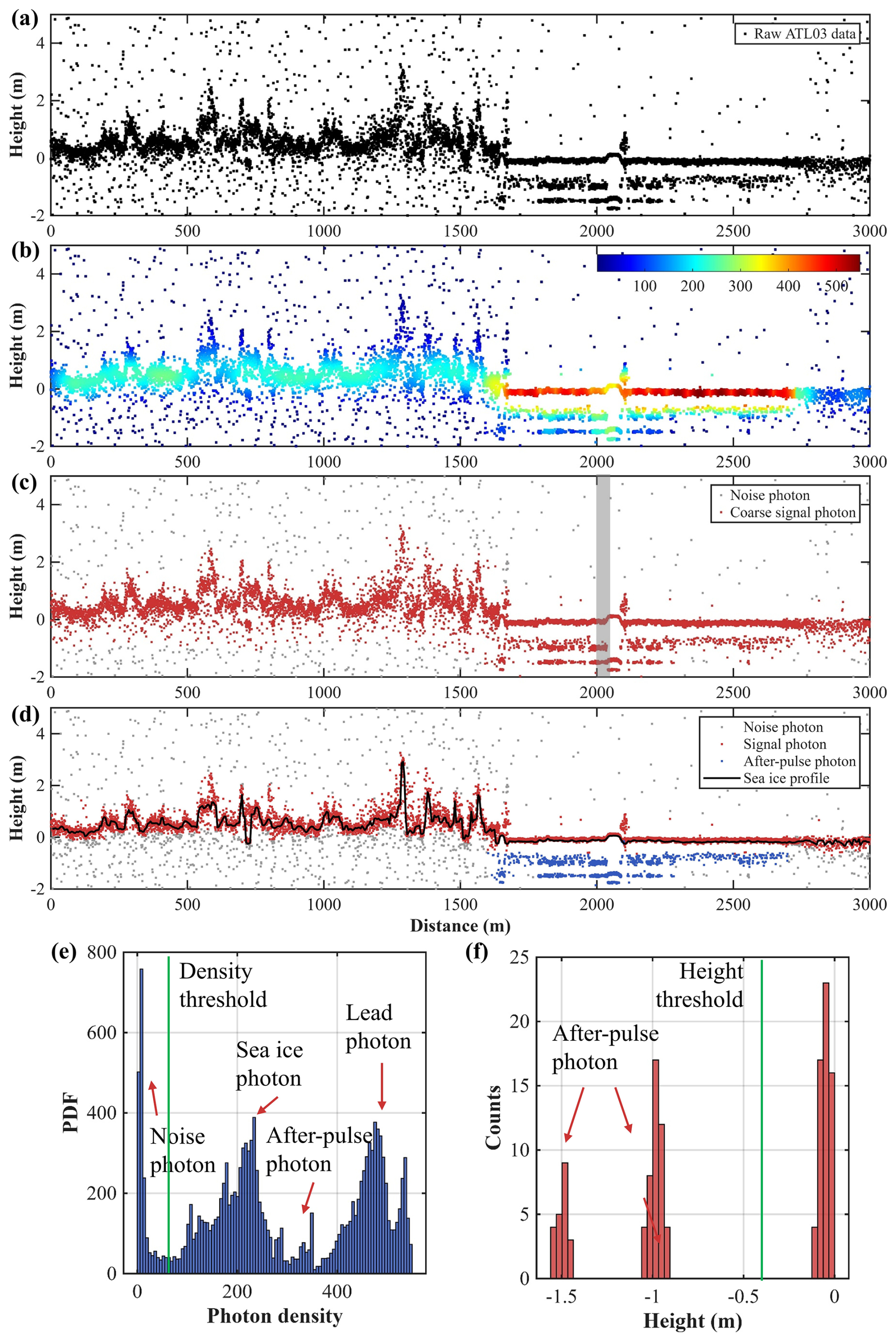
Figure A1 Same as Fig. 3, but for the weak beam of ATL03_20190526002946_08820304_006_02 over the Lincoln Sea.

Figure A2 Same as in Fig. 3, but for a melt pond example.

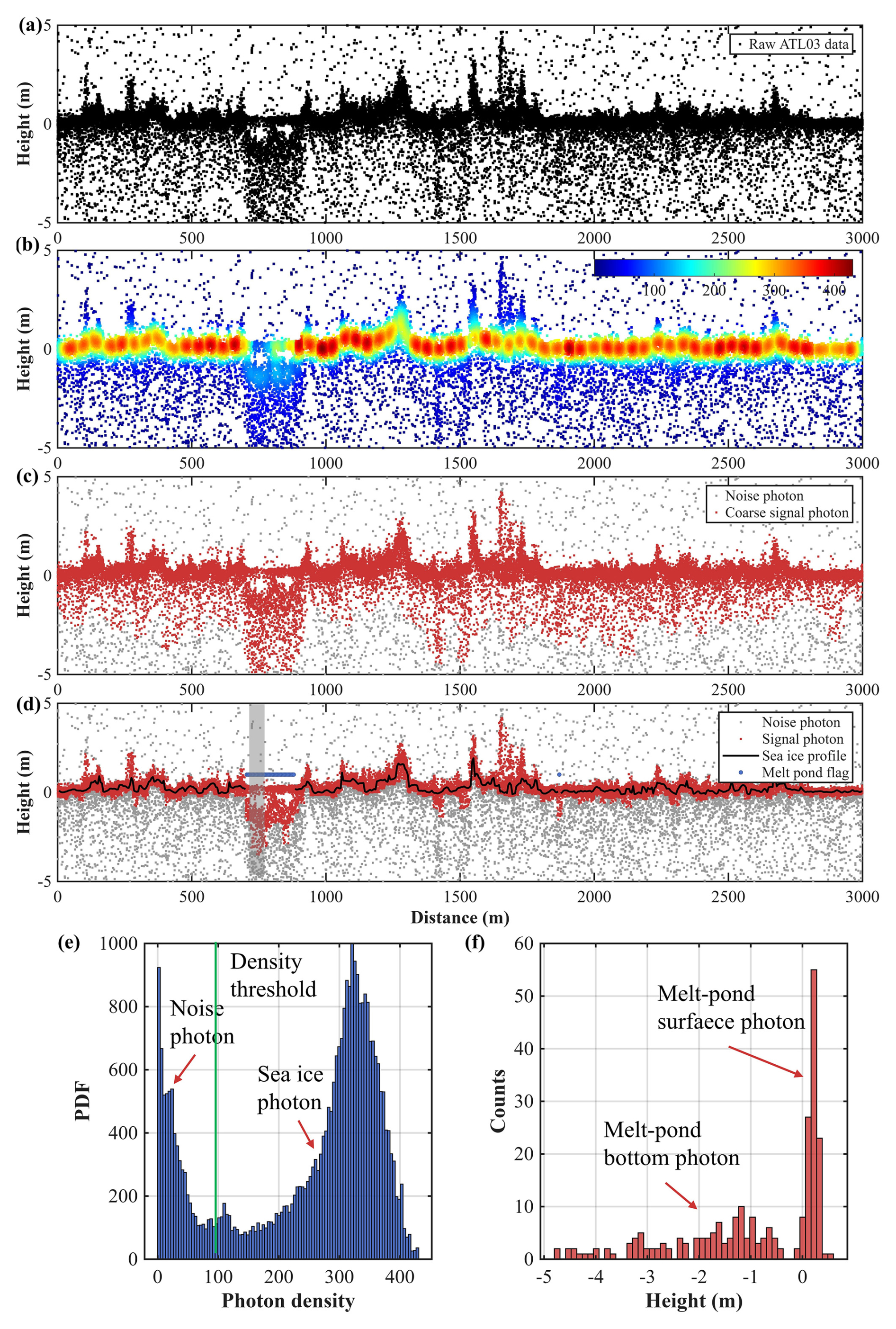
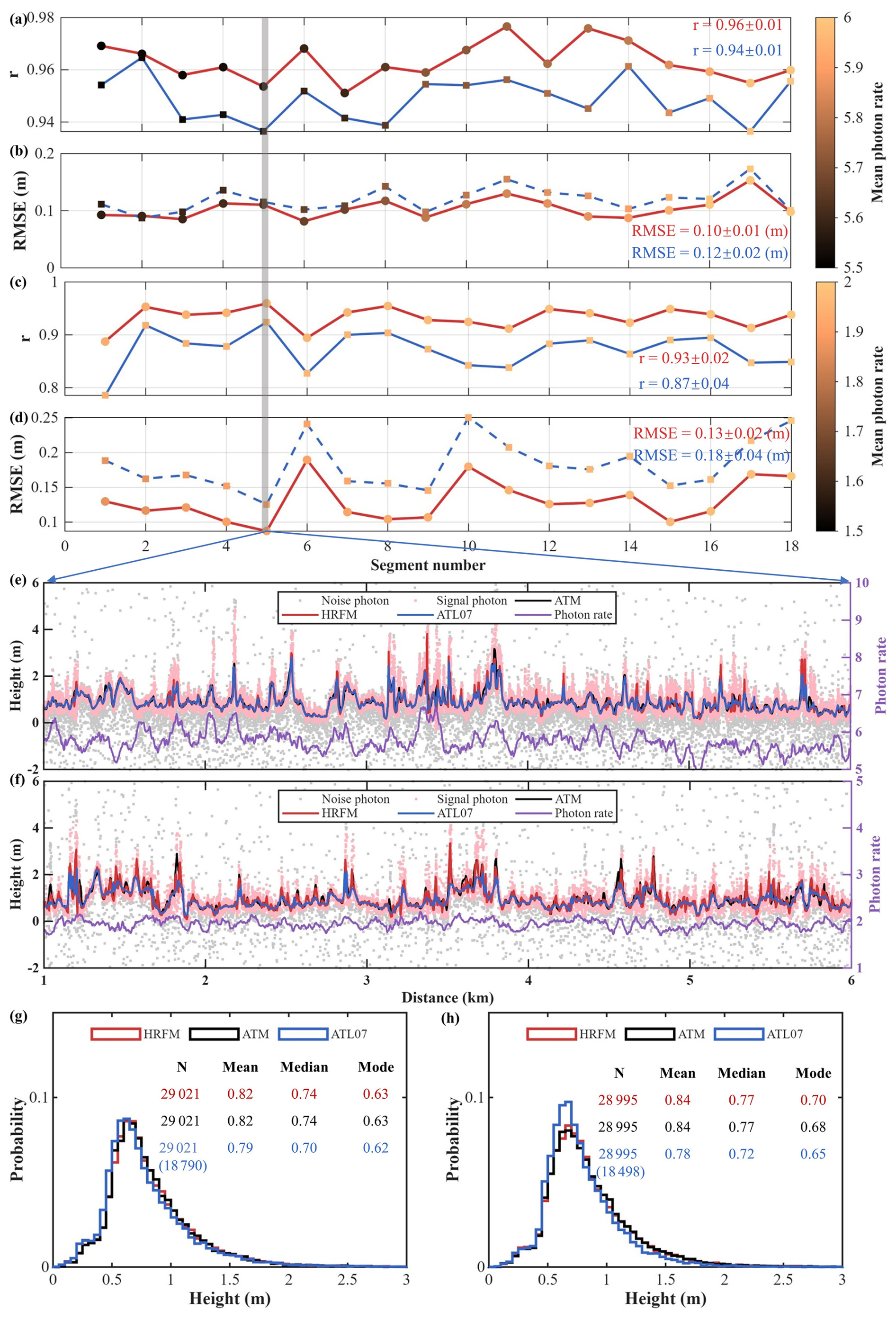
Figure A3 Same as in Fig. 7, but for ATM observations acquired on 8 April 2019. The statistics are computed from 18 along-track segments.

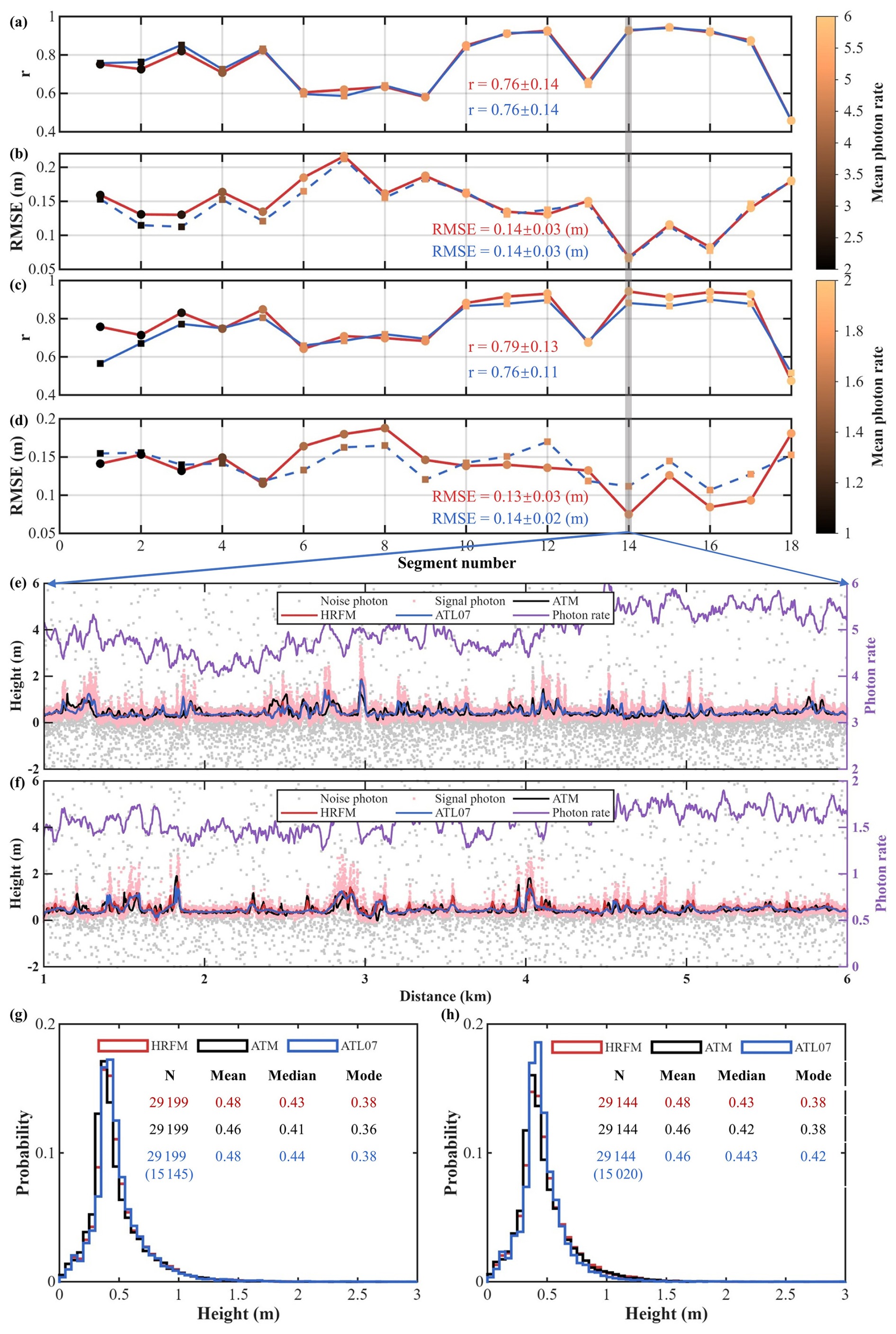
Figure A4 Same as in Fig. 7, but for ATM observations acquired on 12 April 2019. The statistics are computed from 18 along-track segments.

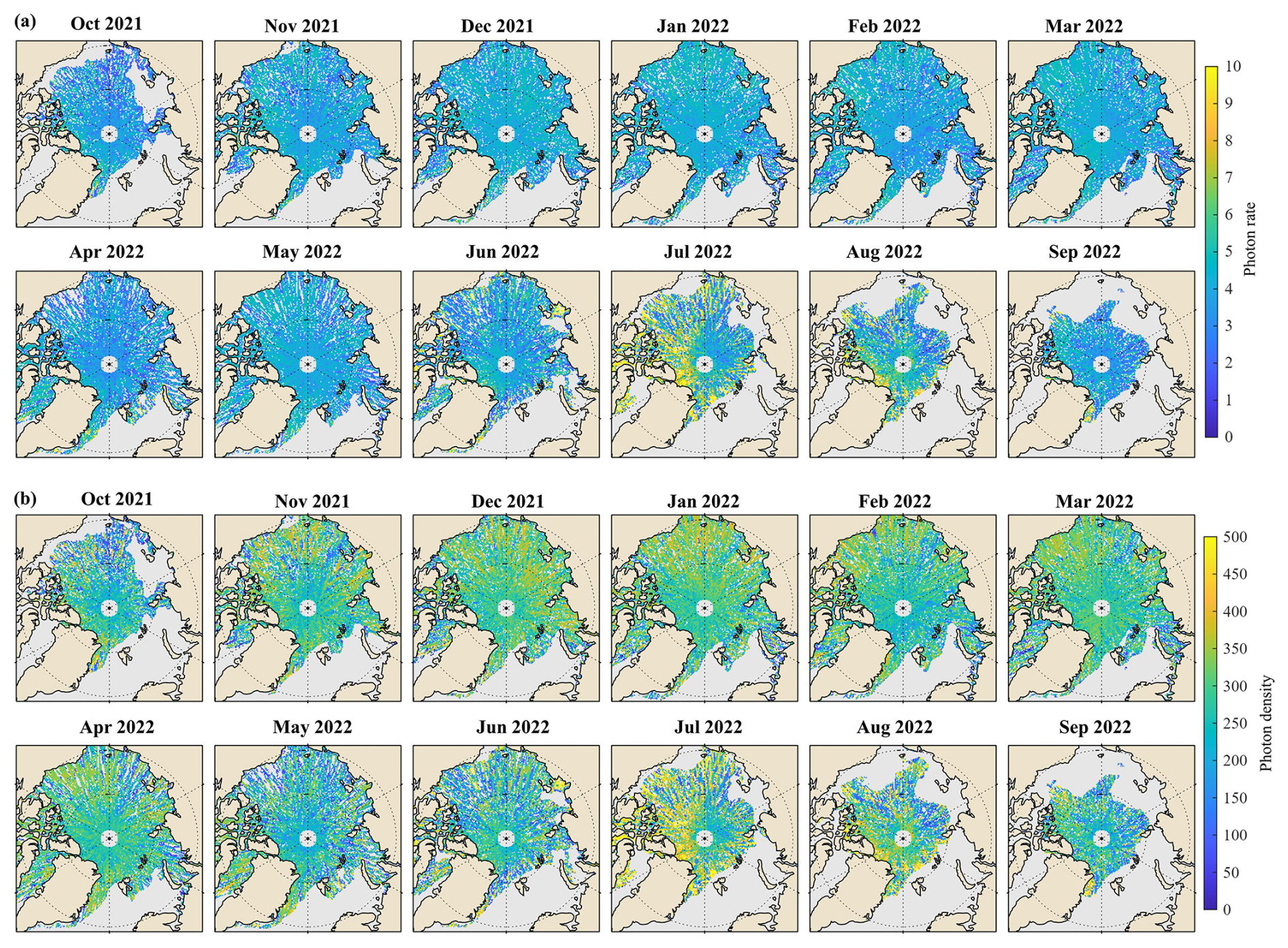
Figure A5 Monthly distributions of HRFM classification features from October 2021 to September 2022. (a) Monthly mean photon rate and (b) monthly mean photon density on the 25 km Arctic grid.

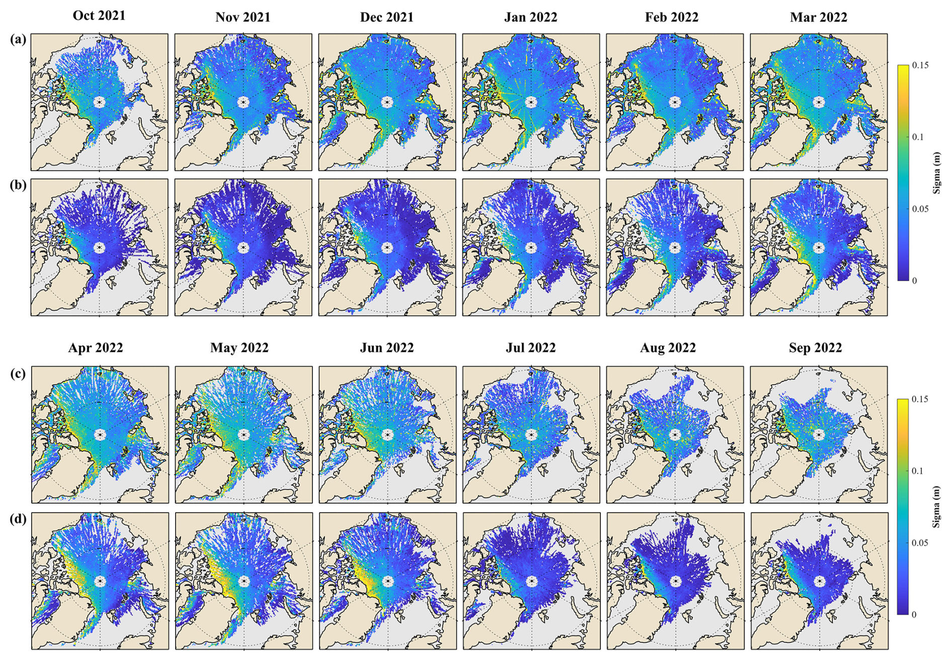
Figure A6 Monthly standard deviation of sea-ice freeboard within each 25 km grid cell from October 2021 to September 2022 for (a, c) HRFM and (b, d) ATL20.

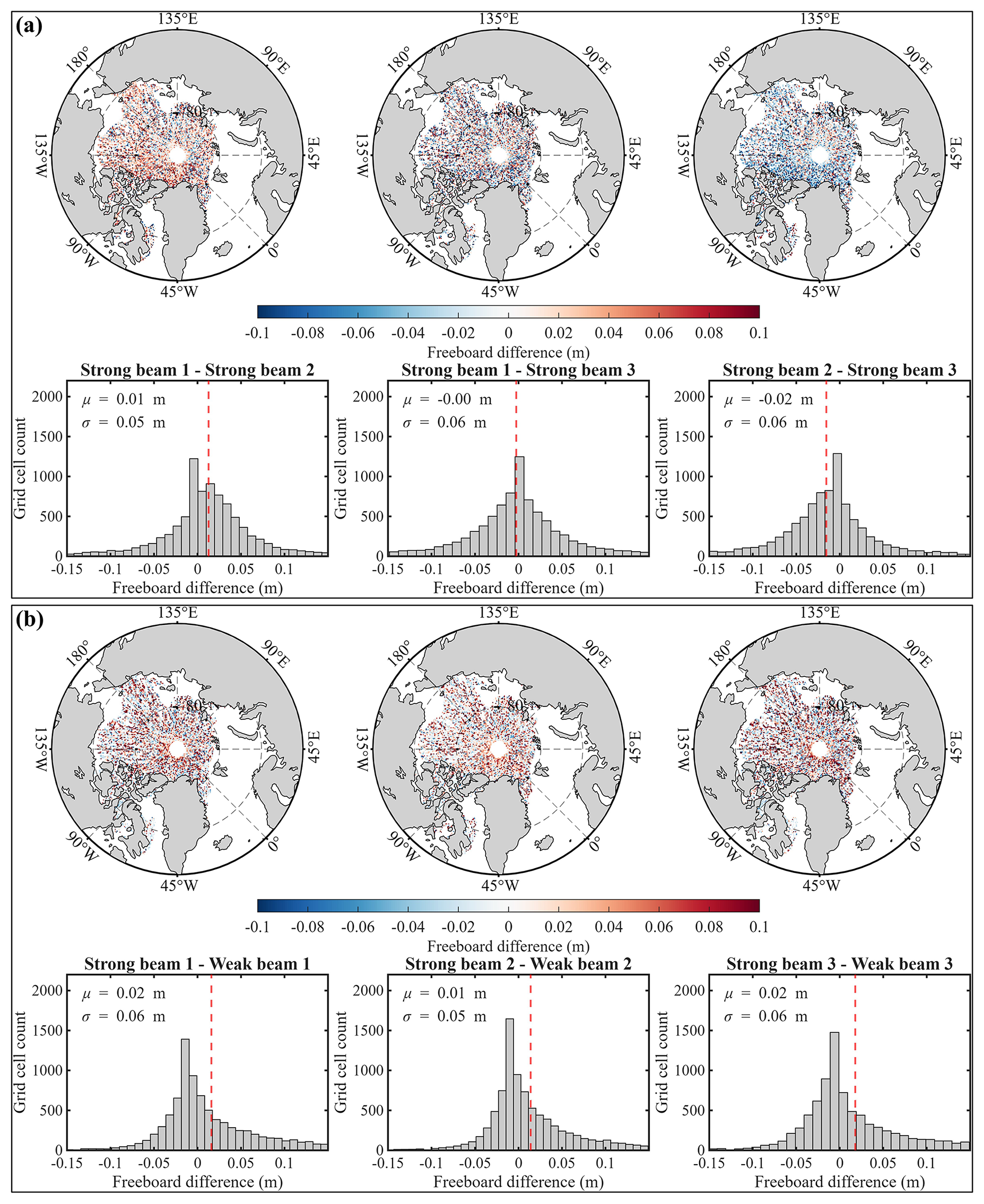
Figure A7 Same as in Fig. 11, but for July 2022.