The multilayer ocean circulation melting the 79N Glacier ice tongue

The Greenland Ice Sheet is a major contributor to global sea level rise. While surface melting is driven by the atmosphere, oceanic processes melt the floating glacier tongues in northern Greenland from below. Because direct observations beneath these tongues are limited, numerical models are crucial for a detailed understanding of ice–ocean interactions. To study the oceanic melting of Greenland's largest floating ice tongue and the circulation induced by meltwater, we developed a high-resolution three-dimensional model of the 79° North Glacier fjord (500 m horizontal resolution, 100 adaptive vertical layers). Our simulation reveals that melting at the ice–ocean interface is driven by three distinct subglacial plumes with different signatures in temperature–salinity space. The paths of these buoyant gravity currents are set by the ice topography, particularly basal channels in the ice shelf, and the Coriolis effect. One plume flows around cone-like features in the ice base with dimensions comparable to the Rossby radius, suggesting that these cones may have formed through plume-induced melting. At about 100 to 200 m depth, the plumes detach from the ice and export meltwater out of the fjord toward the open ocean. Heat for melting is supplied by a dense bottom plume flowing into the glacier cavity across the sill at the fjord entrance. Downstream of the sill, hydraulic control leads to enhanced mixing between plume and ambient water, cooling the inflow and reducing the amount of heat that reaches the glacier base. Our model resolves these details of the plumes in the ice cavity, improving the understanding of ocean-driven melt below glacier tongues.

1 Introduction

The Greenland Ice Sheet has lost mass at an accelerated rate since the 2000s, strongly contributing to global sea level rise (Mouginot et al., 2019). About half of the mass loss consists of solid ice discharge (Mankoff et al., 2020b), the other half is surface runoff (Mankoff et al., 2020a). Both, ice and freshwater discharge into the ocean, impact the Atlantic overturning circulation by freshening the upper ocean in the areas of North Atlantic Deep Water formation (Böning et al., 2016).

Mass loss from Greenland's glaciers is strongly influenced by the relatively high water temperatures in the North Atlantic (Straneo and Heimbach, 2013). In the Nordic Seas, the Norwegian Atlantic Current transports warm and salty waters of Atlantic origin northward into Fram Strait. Half of this Atlantic water enters the Arctic Ocean proper, whereas the other half recirculates in central Fram Strait and continues southward as the lower limb of the East Greenland Current (Wekerle et al., 2017). A part of the Atlantic water is transported onto the Northeast Greenland continental shelf, where it mixes with colder Arctic Atlantic Water and forms a water mass called Atlantic Intermediate Water (AIW). AIW then flows in a trough system toward Nioghalvfjerdsbræ, the 79° North Glacier (79NG, Fig. 1a; Münchow et al., 2020), one of the few glaciers on Greenland with a floating ice tongue (Millan et al., 2023b). 79NG features Greenland's largest floating ice tongue, with an area of about 70 km×20 km (Fig. 1b, c; Wilson et al., 2017; Schaffer et al., 2020). Even though the ice tongues in northern Greenland are rather small compared to the hundreds-of-kilometers wide ice shelves around Antarctica, they do have an important buttressing effect on the ice streams feeding into the glaciers. Buttressing impedes the ice flow into the ocean and thereby constrains the mass loss of the Greenland Ice Sheet. The neighboring glacier of 79NG, Zachariæ Isstrøm, lost its floating ice tongue in recent decades (Mouginot et al., 2015), which led to increased calving rates and acceleration of the upstream ice stream (Khan et al., 2022), with implications for global sea level rise.

The fjord of 79NG, Nioghalvfjerd Fjord, extends from the glacier's grounding line in the southwest toward a main calving front in the east and a shorter calving front in the north, located in a side branch of the fjord called Dijmphna Sound (Fig. 1b). Oceanographic measurements at 79NG revealed that the inflow of AIW occurs primarily through the main calving front and not through Dijmphna Sound (Mayer et al., 2000; von Albedyll et al., 2021). The inflow of AIW at the main calving front is steered by the local bathymetry over a sill and through a narrow channel of around 5 km width down into the glacier cavity (Schaffer et al., 2020). The dense inflow forms a strong, bottom-intensified gravity current, called a plume. Measurements with an ice-tethered mooring on the glacier tongue revealed the year-round presence of AIW in the cavity (Lindeman et al., 2020), causing pronounced melt at the ice base. The melting is particularly strong near the grounding line (Wilson et al., 2017; Millan et al., 2023b), where the ice tongue is thick and has a large draft (Fig. 1c). As opposed to the Zachariæ Isstrøm, the extent of the 79NG tongue has been relatively stable in recent years, but it thinned by around 30 % between 1999 and 2014 (Mouginot et al., 2015; Mayer et al., 2018). On the other hand, between 2017 and 2021, a decreased heat transport into the cavity was observed, associated with reduced basal melt rates in this time period (McPherson et al., 2024). This shows that the inflow of AIW and, more generally, the local ocean circulation is important for the melting and the stability of 79NG.

Despite those observational advances, measurement campaigns at 79NG remain difficult due to harsh weather conditions, fast ice often locking the fjord entrance and the hundreds of meters thick ice tongue. Therefore, ocean modeling is crucial for exploring and understanding ice–ocean interactions in the fjord. However, the complex topography poses a challenge to modeling this system, for example, the sill constraining the warm water inflow (Schaffer et al., 2020) and the deep channels in the ice base (Zeising et al., 2024), which strongly impact melt patterns (Rignot and Steffen, 2008; Larter, 2022; Chartrand et al., 2024; Mohammadi-Aragh et al., 2025). Basal channels guide fast currents along the underside of the glacier tongue, so-called subglacial plumes (Hewitt, 2020). To accurately represent the plume dynamics and the induced basal melting, a numerical model must provide a sufficiently high resolution within these plumes.

Not only the horizontal distribution, but also the vertical structure of the subglacial plumes has a strong impact on ocean-driven basal melting, due to the role of the interfacial friction velocity in the melt formulation (Hellmer and Olbers, 1989). The entrainment layer separating the cold and fresh plume from the warmer and saltier ambient water below needs to be properly resolved to reproduce the plume water's insolation effect on the ice. In a one-dimensional plume study, Burchard et al. (2022) found that the vertical resolution of the subglacial plume region should be finer than 2 m. Due to the large range of depths of the ice–ocean interface in subglacial cavities (e.g., 600 m at 79NG), such a high resolution can hardly be achieved in ocean models with geopotential (z-)coordinates as used by, e.g., Losch (2008) or Wekerle et al. (2024). Still, these models typically calculate realistic melt rates, presumably due to feedback mechanisms (unresolved plumes result in higher temperatures under the ice but lower interfacial friction velocities).

To provide a good resolution of subglacial meltwater plumes, models with surface following σ-coordinates have been developed (Dinniman et al., 2007; Gwyther et al., 2020). For the global ocean, Timmermann et al. (2012) developed a hybrid model with terrain-following σ-coordinates inside and close to the ice cavity, but geopotential coordinates elsewhere. More flexibility is given by vertically adaptive coordinates, like those developed by Burchard and Beckers (2004) and Hofmeister et al. (2010). Adaptive coordinates allow for spatially varying and temporally evolving refinement of vertical resolution near strong stratification such as entrainment layers (e.g., the plume interface), but also provide high vertical resolution at the sea surface and the seafloor. Thanks to these features, adaptive vertical coordinates are often used in numerical studies of estuaries and coastal seas (Henell et al., 2023; Li et al., 2024; Lorenz et al., 2025; Burchard et al., 2025). In an idealized two-dimensional (longitudinal–vertical) model of the 79NG cavity, Reinert et al. (2023) demonstrated that both, the cold and fresh subglacial plume as well as the warm and salty bottom-attached AIW plume, can be properly resolved by this method. In realistic simulations of a fjord with a glacier tongue, however, this concept has not been employed yet.

The present study employs the method of vertically adaptive coordinates in a three-dimensional model of the 79NG fjord with realistic bathymetry, ice topography and oceanic forcing to unravel the circulation in the cavity under the floating ice tongue. Our model uses state-of-the-art turbulence and melt parametrizations that are suitable for high resolutions. This allows to accurately represent the subglacial plumes and their role in melting the glacier from below. Also the AIW plume dynamics are properly resolved by this approach, enabling us to analyze the inflow using classical gravity current theory. Furthermore, we consider the combined effect of in- and outflowing plumes, analyzing the exchange flow between cavity and open ocean, using the Total Exchange Flow (TEF) framework in temperature and salinity coordinates. Together, these results present a detailed picture of ice–ocean interactions in the 79NG cavity and resolve processes in a realistic simulation that have so far only been described in theoretical or idealized settings.

This paper is structured as follows: Our model setup, forcing and analysis methods are explained in the following Sect. 2. The simulation results are shown and compared with observations in Sect. 3, with focus on melting and the subglacial plume dynamics (Sect. 3.2 and 3.3). The implications of our results are discussed in Sect. 4, followed by concluding remarks in Sect. 5.

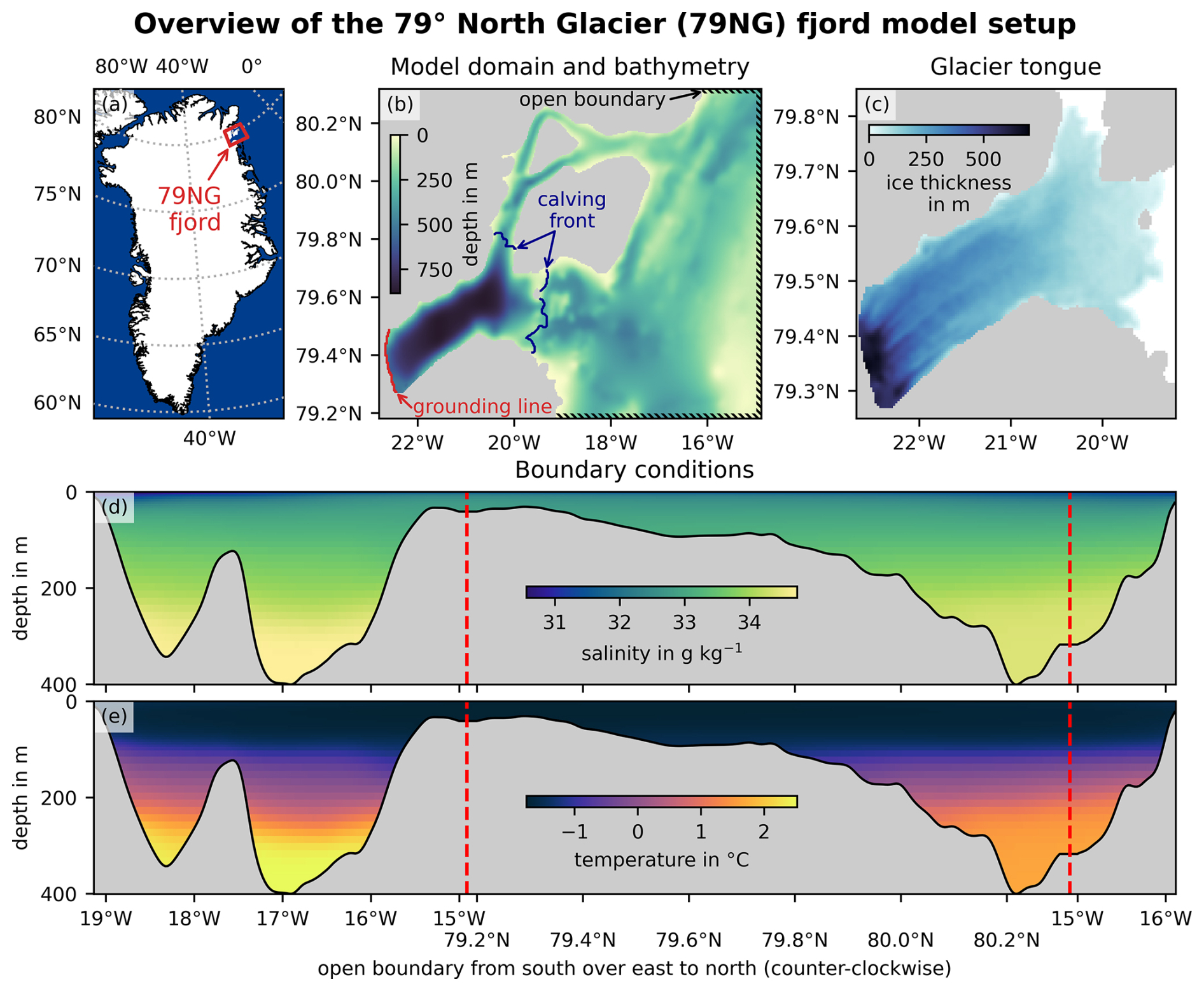
Figure 1 (a) Location of the 79NG fjord in Greenland. (b) Model domain and bathymetry; the northern branch of the fjord is Dijmphna Sound; subglacial discharge enters through the grounding line, which is the landward end of the floating glacier tongue; the calving front is its seaward end. (c) Thickness of the floating 79NG tongue. (d) Salinity and (e) temperature boundary conditions of the model; the open boundary (hatched area in panel b) is shown “unwinded” in counter-clockwise direction with the red dashed vertical lines marking the transitions between the southern, eastern and northern boundaries.

2 Methods

2.1 High-resolution model of the 79NG fjord

We built a high-resolution numerical model of the 79NG fjord (Fig. 1) using the coastal ocean model GETM (Burchard and Bolding, 2002). GETM is a hydrodynamic model that computes currents and transports with the three-dimensional equations of motion under the Boussinesq approximation. In particular, GETM resolves the flow in the glacier cavity below the floating ice tongue. Since the 79NG tongue has a gentle slope of only about 2 % on average, and a much greater horizontal than vertical extent, it is appropriate to use the classical hydrostatic mode of GETM, instead of the computationally more demanding non-hydrostatic extension (Klingbeil and Burchard, 2013). The glacier tongue is implemented by accounting for the melt fluxes at the ice–ocean interface, the friction between ice and ocean, and the additional pressure due to the weight of the tongue. Note that we do not employ an ice sheet model and use a constant-in-time ice thickness, since the timescales over which the ice evolves are longer than those of the oceanic flow (Hewitt, 2020). Nevertheless, the vertical position of the floating ice and the free surface may change in response to propagating long waves and varying seawater density. The implementation details of glacier ice in GETM are explained by Reinert et al. (2023).

The employed melt formulation is a numerically consistent implementation (Burchard et al., 2022) of the classical three-equation model for volume and temperature fluxes across the ice–ocean interface (Holland and Jenkins, 1999). Numerically consistent means that the melt fluxes converge to their analytical values and the velocity directly at the ice converges to zero for increasing resolution. This is achieved by using a resolution-dependent formulation of the drag coefficient at the ice base, derived from the law of the wall:

$$\begin{array}{}\text{(1)}& c_{\mathrm{d}}={\left[{\displaystyle \frac{\mathit{\kappa }}{\ln \left(\frac{\frac{\mathrm{1}}{\mathrm{2}}{h}_{k_{\max }}+z_{\mathrm{0},\mathrm{ice}}}{z_{\mathrm{0},\mathrm{ice}}}\right)}}\right]}^{\mathrm{2}},\end{array}$$

where $h_{k_{\max }}$ is the thickness of the uppermost model layer, $z_{\mathrm{0},\mathrm{ice}}=\mathrm{0.01}\mathrm{m}$ is the ice roughness length, and κ=0.4 is the von Kármán constant. For increasing vertical resolution with $h_{k_{\max }}\to \mathrm{0}$, the drag coefficient c_d increases infinitely, such that the velocity in the uppermost model layer converges to zero. See Burchard et al. (2022) for further details; regarding the ice roughness length sensitivity, see also Reinert et al. (2023).

For an accurate computation of the melt rate, the vertical resolution should be finer than 2 m in the subglacial plume flowing along the ice (Burchard et al., 2022). Such a high resolution is achieved in GETM by using adaptive vertical coordinates (Hofmeister et al., 2010). These topography-following coordinates automatically adjust the distribution of the vertical layers in response to the current state of the system (Burchard and Beckers, 2004). The vertical resolution increases dynamically in places of interest: the ice–ocean interface, the seafloor, and – importantly – stratified areas (Reinert et al., 2023). This is implemented by letting the vertical distribution of the model layers evolve over time, where the layer spacing is a function of the vertical density gradient and the vertical distance from the boundaries, see Burchard and Beckers (2004) and Hofmeister et al. (2010) for the mathematical details. This results in a “zooming toward stratification”, which allows resolving the meltwater currents at the ice–ocean boundary with about 1 m vertical resolution over the whole ice tongue, and also the inflowing plume of warm water is well-resolved. Our setup uses 100 adaptive vertical coordinate layers.

In the horizontal, our model uses a regular latitude–longitude grid with a resolution of about 500 m (precisely: ($\mathrm{1}/\mathrm{240}$)° = 0.00417° in latitude, ($\mathrm{6}/\mathrm{240}$)° = 0.025° in longitude). The model grid consists of 312×273 cells, i.e., about 85 000 grid cells in total, 56 % of which are water points (Fig. 1b). The timestep of our model is 2 s for the barotropic (vertically integrated) mode, in accordance with the CFL stability condition, and 30 s for the baroclinic (vertically resolved) mode, i.e., the split factor between the two modes is M=15. The setup uses the Smagorinsky parameterization of the horizontal momentum diffusion and state-of-the-art vertical turbulence closure with GOTM (Burchard et al., 1999; Umlauf and Burchard, 2005).

2.2 Bottom and ice topography

The bottom topography of our setup (Fig. 1b) comes from RTopo-2.0.4 (Schaffer et al., 2019). In the creation of this dataset, particular attention was paid to the bathymetry of the 79NG fjord. Importantly, data of a recent bathymetric survey covering the fjord mouth (Schaffer et al., 2020) were incorporated in RTopo-2.0.4. Furthermore, we verified that the RTopo-2.0.4 bathymetry fits the seismic depth soundings of the ice-covered 79NG cavity (Mayer et al., 2000). RTopo has a horizontal resolution of $\mathrm{1}/\mathrm{120}$°, corresponding to a meridional resolution of about 930 m and a zonal resolution of 155 to 175 m at 79NG.

Regarding ice thickness, RTopo is rather smooth and lacks details, so instead we use the more detailed BedMachine Version 5 (Morlighem et al., 2022, 2017) for the topography of the floating ice tongue (Fig. 1c). BedMachine has a nominal horizontal resolution of 150 m, includes more recent measurements of the ice thickness and shows more features in the ice than RTopo. In particular, melt channels in the glacier tongue are visible in BedMachine, which are an important feature impacting currents and melting at the underside of the floating ice tongue (Mohammadi-Aragh et al., 2025). These channels are typically between 500 m and a few kilometers wide (Rignot and Steffen, 2008; Sergienko, 2013; Zeising et al., 2024), so the larger basal channels are resolved in our model. In the vicinity of the grounding line, BedMachine contains smoothed data as a result of blending datasets from different sources: a mass conservation approach was used for fast-flowing grounded ice, gravity inversion was used for the floating ice tongue, and both data sources were connected smoothly by interpolation (Morlighem et al., 2017). This results in a less detailed ice topography and no channels visible in this area (see the western end of the ice tongue in Fig. 1c). Since the well-established BedMachine dataset provides a consistent topography of the whole floating ice tongue, we did not blend the data with recent high-resolution ice thickness measurements around the grounding line (Zeising et al., 2024).

2.3 Boundary and initial conditions

Our model domain extends from the grounding line in the southwest through the whole 79NG fjord, including the northern branch Dijmphna Sound, and ends at a three-sided open boundary on the continental shelf (Fig. 1b). The open boundary is located in the south at 79.2° N, in the north at 80.3° N, and in the east at 15° W. At these boundaries, we prescribe realistic long-term averaged temperature and salinity conditions (Fig. 1d, e) that come from a global run of the ocean model FESOM2.1 with increased resolution in the 79NG fjord (Wekerle et al., 2024). The FESOM data were averaged over the ten-year period 2011–2020, to have steady boundary conditions that are similar to the present-day situation. We focus in this paper on the description of the typical circulation in the 79NG fjord, for which a steady forcing seems appropriate. How the results could change under time-varying forcing is discussed in Sect. 4.5.

We do not prescribe tides or velocities at the open boundary, because the tidal velocity in the several hundred meters deep cavity is small compared to the velocity of the plumes, so tides have only a minor impact on the 79NG melt rate (Reinert et al., 2023). This is different from some ice shelves in Antarctica, where melting can be strongly impacted by tides (Richter et al., 2022). Also note that tides affect the floating and grounded 79NG ice by modifying the glacier's sliding speed and increasing the strain, so tidal forcing is relevant to model the flow and deformation of the glacier ice itself (Christmann et al., 2021). In our model, the oceanic flow below the ice is simulated, but not the ice evolution happening on longer timescales (Hewitt, 2020). Since we focus on processes in the glacier cavity, which is isolated from the atmosphere by the ice tongue, we do not include atmospheric forcing or sea ice in the model (see also Sect. 4.5.2).

Oceanographic measurements taken with moorings at the 79NG fjord entrance in 2016/2017 suggest that the subglacial runoff discharged at the grounding line is about Q_runoff=0.07 mSv (milli-Sverdrup, $\mathrm{1}\mathrm{mSv}={\mathrm{10}}^{\mathrm{3}}{\mathrm{m}}^{\mathrm{3}}{\mathrm{s}}^{-\mathrm{1}}$) in annual mean (Schaffer et al., 2020). This freshwater input is included in our setup, uniformly distributed along the 25 km-long grounding line (Fig. 1b). Even though subglacial discharge is more likely to cross the grounding line through discrete channels (Narkevic et al., 2023), rather than widely distributed (Hewitt, 2020), we did not use channelized discharge in our model, since the BedMachine ice topography does not show channels in the grounding zone (see Sect. 2.2). However, we discuss the possible implications of this simplification in Sect. 4.5.1. Both the subglacial discharge at the grounding line and the ocean-driven basal melting of the ice tongue are implemented in GETM as freshwater fluxes that increase the volume of the corresponding water column (Burchard et al., 2022; Reinert et al., 2023). This implementation is more realistic than the often employed alternative of using virtual salt fluxes (Huang, 1993).

Initiating the setup with conditions from the same FESOM simulation that is used as boundary data, we let the simulation spin up for five years. At the end of the spin-up phase, the model has reached a quasi-steady state, where melt rate, surface elevation, and barotropic kinetic energy do not fluctuate much anymore. The spatial mean melt rate has converged to a range of 11.2 to 11.5 m yr⁻¹. In this study, we show results averaged over one simulation year after the five-year spin-up. As the model forcing comes from a realistic global ocean simulation, we consider this one-year average after the spin-up to be a representative quasi-steady state of the 79NG fjord at present-day. Averaged results were computed on the model timestep, i.e., numerically exact. Standard deviations were computed on hourly model snapshots, i.e., using 8760 data points.

2.4 Analysis of the bottom gravity current

Our simulation shows an inflow of dense water as a bottom gravity current, as expected from previous studies (see Sect. 3.4.2). To quantify the properties of this inflowing plume, we follow the method by Schaffer et al. (2020): We consider the inflow as a 2.5-layer system with a well-mixed plume layer at the bottom, mixing with a middle layer above it; the upper part of the water column forms the 0.5-layer not directly impacted by the inflow, as it is separated by the middle layer. The two interfaces between the layers are chosen as two isopycnals, the deeper one at 27.5 kg m⁻³ separating the well-mixed bottom current from the stratified interior, the lighter one at 27.2 kg m⁻³ being relatively horizontal in a rather quiescent part of the water column. Note that this choice of isopycnals is specific for the inflow transect shown in Figs. 5 and 6. We verified that our findings still hold if the density interfaces are varied by up to $\pm \mathrm{0.1}\mathrm{kg}{\mathrm{m}}^{-\mathrm{3}}$, and show the plume properties also for a second isopycnal in Fig. 6, to give an idea of their sensitivity.

With this definition, the plume in the transect consists of all water with densities of 27.5 kg m⁻³ and above, and the plume thickness D_plume(x,y) is the height above ground of this isopycnal. The density of each layer can be computed by integrating the density $\mathit{\rho }(x,y,z)$ over the layer and dividing by the layer thickness, e.g., for the plume density:

$$\begin{array}{}\text{(2)}& {\mathit{\rho }}_{\mathrm{plume}}(x,y)={\displaystyle \frac{\mathrm{1}}{D_{\mathrm{plume}}}}\underset{-H}{\overset{-H+D_{\mathrm{plume}}}{\int }}\mathit{\rho }(x,y,z)\mathrm{d}z,\end{array}$$

where $H=H(x,y)>\mathrm{0}$ is the depth of the seafloor, and similarly for the density of the middle layer, ρ₀(x,y) (Schaffer et al., 2020). Given the average density of each layer, the plume buoyancy is

$$\begin{array}{}\text{(3)}& b(x,y)=-g{\displaystyle \frac{{\mathit{\rho }}_{\mathrm{plume}}-{\mathit{\rho }}_{\mathrm{0}}}{{\mathit{\rho }}_{\mathrm{0}}}}\end{array}$$

with the gravitational acceleration $g=\mathrm{9.81}\mathrm{m}{\mathrm{s}}^{-\mathrm{2}}$. The buoyancy is negative, since the inflowing plume is denser than the ambient water.

We can then compute the Froude number of the plume as

$$\begin{array}{}\text{(4)}& \mathrm{Fr}={\displaystyle \frac{u_{\mathrm{plume}}}{\sqrt{-b{D}_{\mathrm{plume}}}}}.\end{array}$$

This non-dimensional number relates the plume velocity along the transect u_plume, computed analogously to Eq. (2), to the phase speed of long waves traveling at the interface between plume and middle layer (Reinert et al., 2023; Burchard et al., 2022; Arneborg et al., 2007). Froude numbers larger than one, Fr>1, mean that the plume flows faster than gravity waves propagate in the opposite direction. This is called supercritical flow and shows that the inflow is limited by hydraulic control. Hydraulic control at the fjord mouth can limit the heat transport into the glacier cavity, with implications for melting and glacier stability (Wiskandt et al., 2025b; McPherson et al., 2024; Nilsson et al., 2023; Schaffer et al., 2020), see Sects. 3.4 and 4.1.

2.5 Overturning stream functions

To analyze the overturning circulation in the 79NG fjord, we compute the overturning stream function, integrated meridionally from the southern to the northern fjord wall. We consider the stream function in depth coordinates as well as in tracer coordinates for the tracers salinity and temperature. Both tracers generally increase with depth at 79NG.

The depth–longitude stream function is defined by

$$\begin{array}{}\text{(5)}& Q_z(x,z)=\underset{y_{\mathrm{south}}}{\overset{y_{\mathrm{north}}}{\int }}\underset{-H}{\overset{z}{\int }}u(x,y,z^{\prime })\mathrm{d}{z}^{\prime }\mathrm{d}y,\end{array}$$

where u is the zonal velocity and x, y, z denote the eastward, northward, upward coordinates, respectively. Analogously, the tracer–longitude stream function of a tracer C is defined by

$$\begin{array}{}\text{(6)}& Q_C(x,C)=\underset{c>C}{\iint }u(x,y,z)\mathrm{d}A,\end{array}$$

as the integral over the area in the y–z plane where c>C, i.e., the area where the tracer concentration $c(x,y,z)$ is greater than the tracer coordinate C. Some authors (e.g., Döös et al., 2012; Zika et al., 2012) employ a definition similar to Eq. (6) but with c≤C, in which case the sign of the stream function changes. Here, we integrate over areas above a given tracer value, so that the stream functions in tracer coordinates have the same signs as in depth coordinates.

To analyze the zonal exchange flow between cavity and ocean in temperature–salinity (T–S) space, we first define a stream function that considers both tracers simultaneously:

$$\begin{array}{}\text{(7)}& Q_{ST}(x,S,T)=\underset{t>T,s>S}{\iint }u(x,y,z)\mathrm{d}A.\end{array}$$

In the following, we omit the explicit notation of the eastward position x for simplicity, keeping in mind that the equations hold for any given meridional transect. Then, the volume transport per salinity and temperature class is analytically defined as

$$\begin{array}{}\text{(8)}& q(S,T)=-{\displaystyle \frac{{\partial }^{\mathrm{2}}{Q}_{ST}(S,T)}{\partial S\partial T}},\end{array}$$

i.e., the second derivative of the two-dimensional tracer stream function with respect to each tracer (Lorenz et al., 2020). Drawn in a T–S diagram, q(S,T) shows how much each water mass contributes to the exchange flow, see Sect. 3.6.

Note that q(S,T) is the boundary transect term in the water mass transformation framework of Hieronymus et al. (2014) and Groeskamp et al. (2019). Also note that the 2D tracer stream function of Eq. (8) differs from the thermohaline stream function defined by Döös et al. (2012) and Zika et al. (2012), despite the fact that both are stream functions that depend on salinity and temperature. In contrast to their global analysis resulting in one stream function for the entire World Ocean, we use one stream function for each meridional transect of the fjord, considering the transport perpendicular to the transect.

Numerically, the volume transport per salinity and temperature class, q(S,T), is computed from hourly, three-dimensional model output. At each longitude, the zonal volume transport of each grid cell is sorted into temperature–salinity bins, using the Python package pyTEF, which implements the methods described by Lorenz et al. (2019) and Lorenz et al. (2020).

2.6 Bulk value quantification in the Total Exchange Flow analysis framework

To quantify the exchange flow between the 79NG fjord and the open ocean with simple bulk values, we apply the Total Exchange Flow (TEF) analysis framework (MacCready, 2011; Lorenz et al., 2019) in salinity and temperature coordinates. The TEF framework is often used to analyze estuaries, and glacier fjords can be considered a special type of estuary (Straneo and Cenedese, 2015). TEF combines the tracer-space analysis of Walin (1977, 1982) with the bulk-value approach of Knudsen (1900).

The bulk values of in- and outflow are found by evaluating the extrema of the one-dimensional tracer stream function Q_C defined in Eq. (6), see Lorenz et al. (2019). The minimum and maximum points of the tracer stream function are called dividing tracer values, because they mark the transition(s) between in- and outflowing water masses. If the exchange flow in tracer coordinates consists of exactly two layers, then there is a single dividing tracer value between in- and outflow. At 79NG, the inflow is primarily westward, so u<0 for inflowing water (opposite sign than in typical estuarine analyses). In this case, the dividing tracer value C_div is given by the minimum point of the stream function: $Q_C\left(C_{\mathrm{div}}\right)=min\left(Q_C\right)$.

The definition of the stream function Q_C in Eq. (6) implies that

• Q_C(C_max)=0, i.e., the stream function vanishes for the maximum tracer value (which is usually at the seafloor);

• $Q_C\left(C_{\min }\right)=Q_{\mathrm{melt}}+Q_{\mathrm{runoff}}$, i.e., the stream function is equal to the total volume outflow for the minimum tracer value (usually at the sea surface).

Here, Q_melt>0 is the integrated melt rate from the grounding line to the chosen transect. Using these two properties, the inflow into the cavity and the outflow out of the cavity can be quantified with (Lorenz et al., 2019)

$$\begin{array}{}\text{(9)}& {\displaystyle }\begin{array}{rl}{Q}_{\mathrm{in}}& =\underset{C_{\mathrm{div}}}{\overset{C_{\max }}{\int }}-{\displaystyle \frac{\partial Q_C}{\partial C}}\mathrm{d}C\\ & =-Q_C\left(C_{\max }\right)-\left(-Q_C\left(C_{\mathrm{div}}\right)\right)\\ & =Q_C\left(C_{\mathrm{div}}\right)<\mathrm{0},\end{array}\text{(10)}& {\displaystyle }\begin{array}{rl}{Q}_{\mathrm{out}}& =\underset{C_{\min }}{\overset{C_{\mathrm{div}}}{\int }}-{\displaystyle \frac{\partial Q_C}{\partial C}}\mathrm{d}C\\ & =-Q_C\left(C_{\mathrm{div}}\right)-\left(-Q_C\left(C_{\min }\right)\right)\\ & =-Q_{\mathrm{in}}+Q_{\mathrm{melt}}+Q_{\mathrm{runoff}}>\mathrm{0}.\end{array}\end{array}$$

Analogously, replacing volume transport by the sum of advective and diffusive tracer transport, we can compute the in- and outflow bulk fluxes, $Q_{\mathrm{in}}^C$ and $Q_{\mathrm{out}}^C$, of a tracer C (Lorenz et al., 2020). Then, the bulk tracer values are defined as the ratio between bulk tracer fluxes and bulk volume fluxes:

$$\begin{array}{}\text{(11)}& C_{\mathrm{in}}={\displaystyle \frac{Q_{\mathrm{in}}^C}{Q_{\mathrm{in}}}},C_{\mathrm{out}}={\displaystyle \frac{Q_{\mathrm{out}}^C}{Q_{\mathrm{out}}}}.\end{array}$$

These bulk values characterize the in- and outflow. They are presented in Sect. 3.5 for salinity, C=S, and temperature, C=T.

3 Results

This section presents the results of our 79NG fjord model in quasi-steady state, starting with a description of the two-dimensional, barotropic flow (Sect. 3.1). We then look at the simulated melt rate and compare it with observations (Sect. 3.2). The following two sections analyze how the melting is driven by the three-dimensional fjord circulation that consists of the subglacial meltwater plumes (Sect. 3.3) and the AIW plume (Sect. 3.4). Finally, we consider the combined effect of these plumes, i.e., the resulting exchange flow and overturning circulation in the fjord (Sect. 3.5), and map their properties in temperature–salinity space (Sect. 3.6).

3.1 Barotropic flow

The barotropic (vertically integrated) flow in the 79NG fjord is, to first order, in geostrophic balance, which means that the primary flow direction is along contours of $f/D$ (Fig. 2). Since the Coriolis frequency f does not vary much over the fjord extending less than 1° in latitude, contours of $f/D$ are essentially parallel to contours of $\mathrm{1}/D$, where D is the water column thickness, i.e., the difference between the depth of the seafloor and the draft of the ice tongue. The strongest barotropic inflow into the cavity passes the main calving front near the sill at the fjord entrance (Fig. 2). Behind the calving front, the barotropic flow follows D-contours toward the north of the cavity. The 100–300 m-contours cross the northern calving front and a small part of the barotropic flow leaves the fjord through Dijmphna Sound, while deeper contours and most of the barotropic flow turn south. The flow recirculates in the cavity, forming a large cyclonic (anti-clockwise) vortex below the ice with a north–south extent of about 25 km, as wide as the fjord mouth, and elongated in western direction toward the grounding line. Along the southern fjord wall, the barotropic flow aligns once more with the contours of water column thickness. It splits near the calving front with one part recirculating in the cavity, whereas the other part leaves the fjord along the southern fjord wall. Deviations of the barotropic flow from geostrophic balance visible in Fig. 2 are mainly due to the baroclinic meltwater plumes, which are described in detail in Sect. 3.3 below.

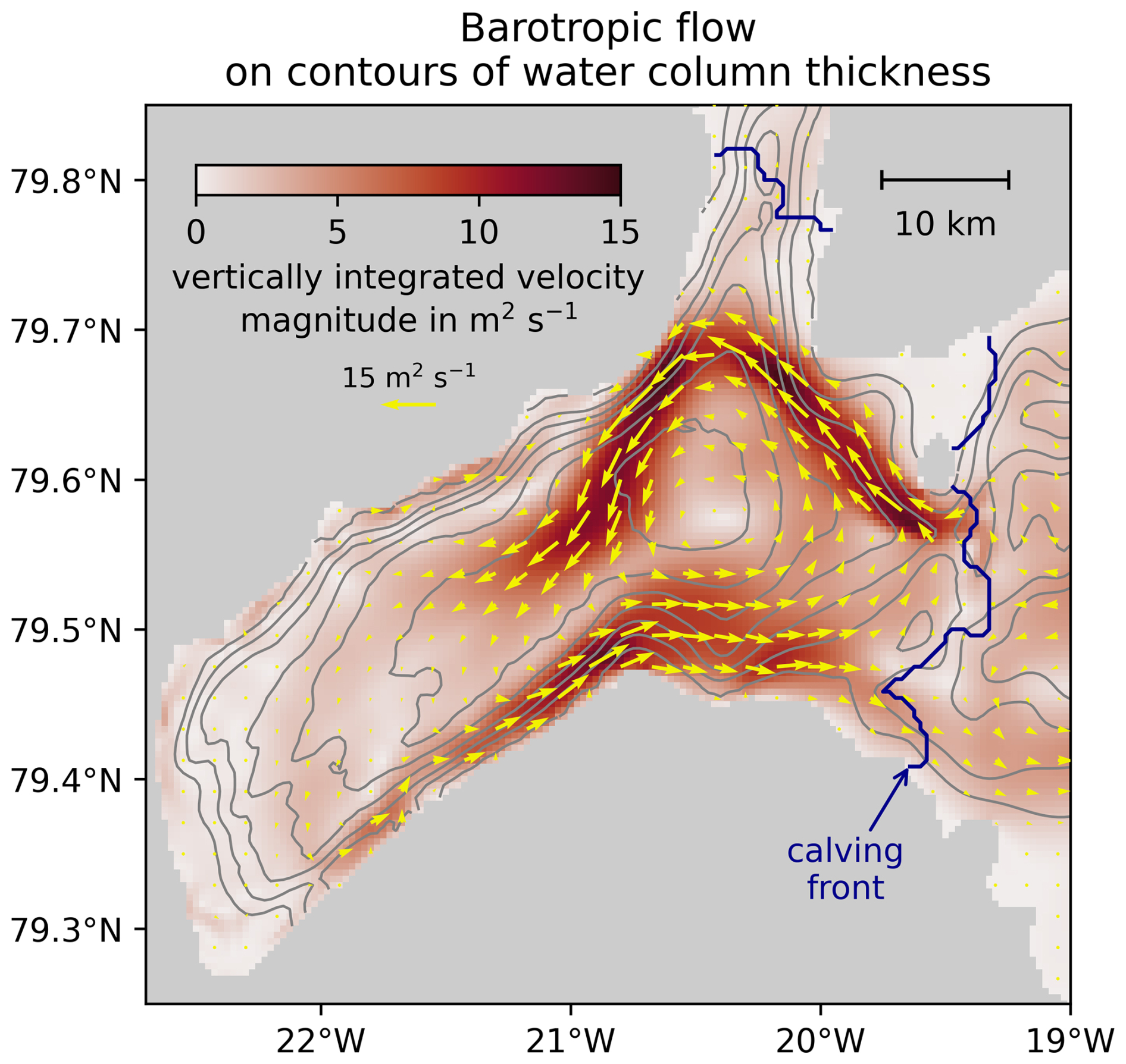
Figure 2 Intensity of the barotropic (i.e., vertically integrated) flow in the 79NG fjord shown in shades of red and the transport direction indicated by yellow arrows. Gray lines are the 100, 200, …, 700 m isolines of the water column thickness, i.e., the depth of the seafloor minus the ice draft; the outermost contour corresponds to 100 m, the closed contour near the center to 700 m.

As most of the barotropic flow recirculates in the cavity, the volume transport (the difference of in- and outflow) across the main calving front is with 5.99 mSv much smaller than the maximum of the barotropic stream function, which is 78 mSv in the center of the vortex, corresponding to the volume transport of the vortex. The outflow through Dijmphna Sound, the northern branch of the fjord, is 6.70 mSv. Thus, the combined transport through both fjord branches is a net volume transport out of the fjord of 0.71 mSv. This value is consistent with the measured outflow of (0.63±0.21) mSv estimated from mooring data in 2016/2017 (Schaffer et al., 2020). The net outflow out of the fjord is, of course, the combination of the subglacial discharge at the grounding line (Q_runoff=0.070 mSv, see Sect. 2.3) and the integrated basal melting in the glacier cavity (Q_melt=0.638 mSv), the distribution of which is described in the following Sect. 3.2.

3.2 Melt rate

The average basal melt rate of the floating 79NG tongue computed by our 3D fjord model is $(\mathrm{11.4}\pm \mathrm{0.1})\mathrm{m}{\mathrm{yr}}^{-\mathrm{1}}$. Integrated over the floating ice tongue, this corresponds to a melt flux of $Q_{\mathrm{melt}}=(\mathrm{0.638}\pm \mathrm{0.003})\mathrm{mSv}=(\mathrm{20.1}\pm \mathrm{0.1}){\mathrm{km}}^{\mathrm{3}}{\mathrm{yr}}^{-\mathrm{1}}$. These values lie well within the error bounds of oceanographic in situ measurements over a one-year period in 2016/2017 that gave $(\mathrm{10.4}\pm \mathrm{3.1})\mathrm{m}{\mathrm{yr}}^{-\mathrm{1}}$ or $(\mathrm{17.8}\pm \mathrm{5.2}){\mathrm{km}}^{\mathrm{3}}{\mathrm{yr}}^{-\mathrm{1}}$ (Schaffer et al., 2020). Our melt rate falls within the higher part of the measurement uncertainty range, presumably due to a slight positive temperature bias in the boundary data used to force our model (Wekerle et al., 2024). Tracer-based measurements yielded a lower melt rate estimate of $(\mathrm{8.6}\pm \mathrm{1.4})\mathrm{m}{\mathrm{yr}}^{-\mathrm{1}}$ (Huhn et al., 2021), but these measurements were conducted during a time of particularly low AIW temperatures, which may explain part of the discrepancy (Kanzow et al., 2025).

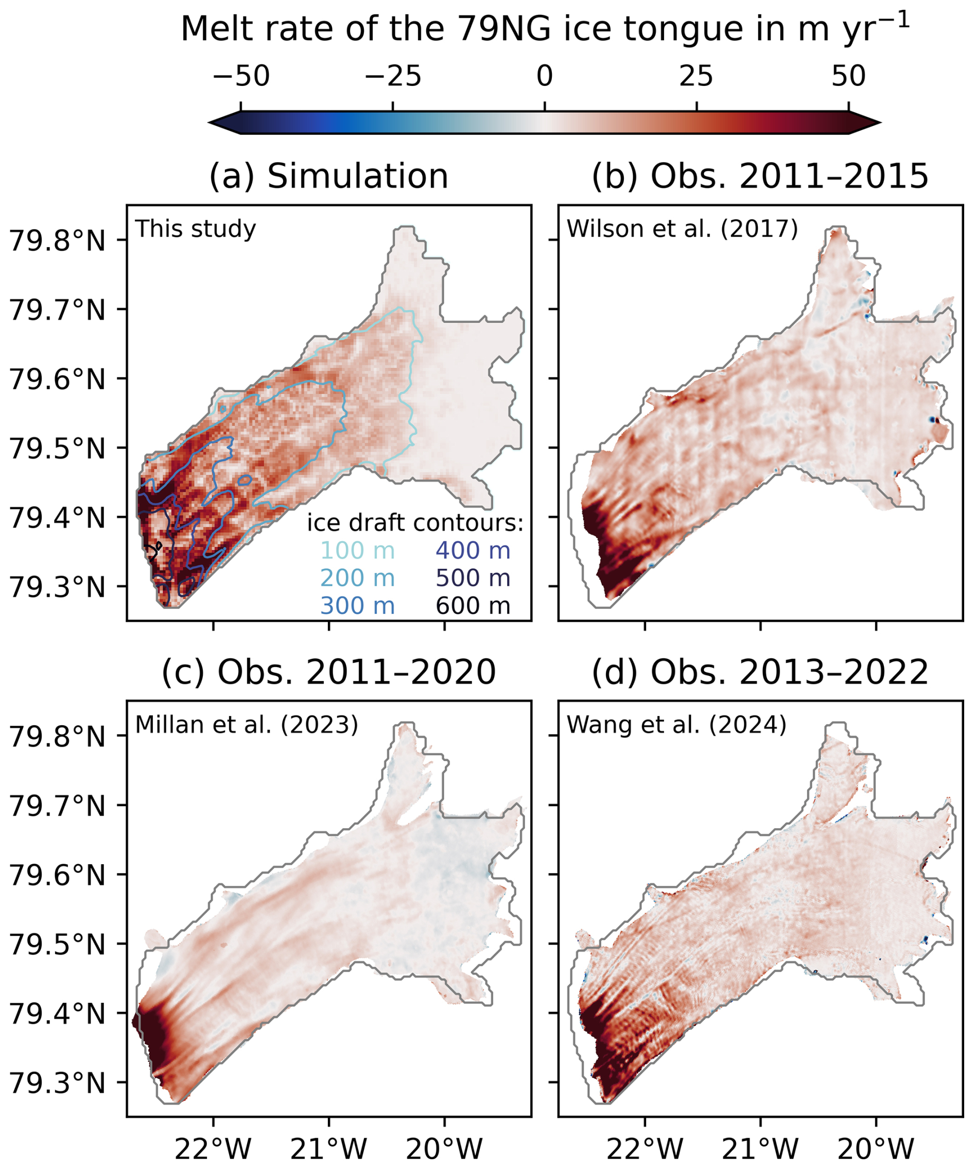
Figure 3 Basal melt rate of the floating 79NG ice tongue computed by the model presented in this paper (panel a), in comparison with melt rates computed from satellite data by Wilson et al. (2017, panel b), Millan et al. (2023b, panel c) and Wang et al. (2024, panel d). Note that the satellite products cover different time periods. The gray contour in each panel is the ice tongue extent in our model.

The basal melt rate varies over the ice tongue in along-fjord (approximately west–east) and in across-fjord (south–north) direction. Regarding the along-fjord variability in our simulation (Fig. 3a), most of the melting occurs at or in the first few kilometers after the grounding line, with a peak melt rate of 104 m yr⁻¹. The melt rate decreases toward the calving front and is essentially zero beyond the 100 m depth contour of the ice draft. There are no negative melt rates in our temporally averaged, quasi-steady state model result; negative melting (i.e., refreezing) only occurs at individual timesteps and only of small amplitude in our simulation. The distribution of basal melting in our model fits well with satellite-based observations by Wilson et al. (2017), Millan et al. (2023b), and Wang et al. (2024), see Fig. 3b–d. Apart from the southwestern part of the ice tongue, the melting appears to be more intense in our model than in the satellite data, but the melt patterns are similar. The hinge zone, which is the part of the ice tongue near the grounding line where the ice is not freely floating, is generally excluded from satellite measurements. However, the hinge zone is also the part where the most extreme melt rates occur (Zeising et al., 2024), so – as pointed out by Kanzow et al. (2025) – the area-averaged melt rate derived from satellite data rather underestimates the total melting. The area-averaged melt rates are 8.2 m yr⁻¹ (Wilson et al., 2017), 4.6 m yr⁻¹ (Millan et al., 2023b), and 8.0 m yr⁻¹ (Wang et al., 2024), and thus smaller than the above-mentioned in situ measurements and our model results. Reasons for the difference are the absence of measurements in the hinge zone, the presence of negative melt rates in the satellite products, and the different temporal ranges covered (Fig. 3).

Also across the fjord, the melting is not uniformly distributed, but high melt rates are focused along specific lanes. This can be seen clearly in high-resolution satellite data (Fig. 3b–d). Our model reproduces these features in the melt distribution and shows that strong melting occurs at the slopes (side walls) of basal channels in the ice tongue (Fig. 3a). This is where subglacial plumes drive the melting, which is explored further in the following Sect. 3.3.

3.3 Subglacial meltwater plumes

Basal melting cools and freshens the top layer of the water column that is in contact with the ice. The water rises up along the ice tongue due to its higher buoyancy, entrains ambient water, and forms the subglacial meltwater plume (Hewitt, 2020). The subglacial plume is fueled by meltwater (and by subglacial discharge at the grounding line), but also influences the melting. On the one hand, the plume can cause more melting by mixing up ambient heat toward the ice and exerting friction on the ice–ocean interface (Burchard et al., 2022). On the other hand, the relatively cold plume water isolates the ice from the warmer ambient water in the cavity, potentially reducing melting. Due to this pivotal role in basal melting, we analyze the subglacial plume in our simulation in detail.

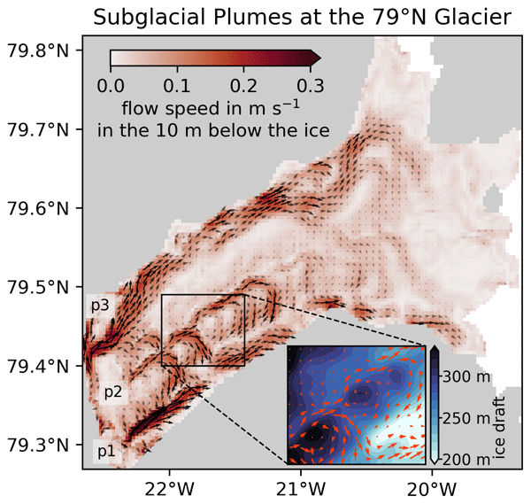
For a first overview of the plume, we consider the average velocity in the 10 m just below the ice (Fig. 4a), since this is a typical thickness of the subglacial meltwater plume (Reinert et al., 2023; Mohammadi-Aragh et al., 2025). Thanks to the adaptive vertical coordinates employed in our model, the upper 10 m of the water column are resolved by at least 6 and on average 12 model layers, so our model achieves the vertical resolution necessary for an accurate melt flux computation (Burchard et al., 2022). The flow speed (Fig. 4a) shows similar spatial patterns as the melting (Fig. 3a), particularly in the part of the cavity where the ice is thick. This confirms that melting and plume strongly influence each other. Three parts of the glacier tongue have particularly fast under-ice flow (labeled p1–p3 in Fig. 4a), which we consider as distinct subglacial plumes and describe further in the following subsections.

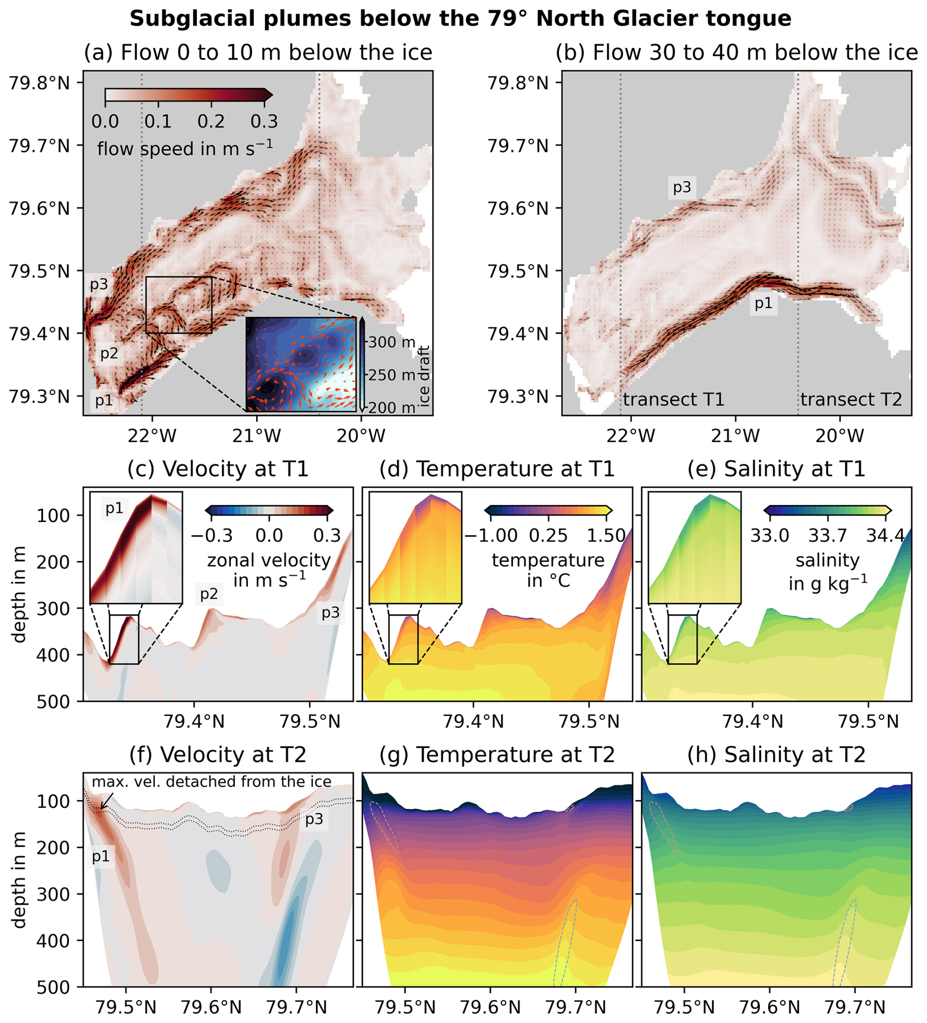
Figure 4 Details of the subglacial meltwater plumes below the 79NG ice tongue: the southern (p1), central (p2) and northern plume (p3). (a) Velocity of the flow averaged over the 10 m directly below the ice tongue; panel (b) is the same for the range of 30 to 40 m below the ice. The inset in (a) shows how the flow turns around cone-like features in the ice topography; the area shown in the inset is about 13 km×10 km wide. For the transect T1 marked in (a) and (b), vertical profiles are shown in (c), (d), (e) for zonal velocity, temperature and salinity, respectively; panels (f)–(h) are analogous for transect T2. Zoomed insets in (c)–(e) show the fine vertical model resolution in the plume. Dotted lines in (f) mark the 30–40 m-range shown in (b). The $\pm \mathrm{0.1}\mathrm{m}{\mathrm{s}}^{-\mathrm{1}}$ velocity contours are shown in (g) and (h) for orientation.

3.3.1 The southern subglacial plume

The first subglacial plume (p1) is located in the south of the cavity, starts near the grounding line in the west, and flows to the calving front in the east (Fig. 4a, b). Initially, the plume does not flow directly along the southern fjord wall, but along the southern side of a channel in the ice (Fig. 4c). This is due to the Coriolis effect, making the plume flow in geostrophic balance with the deeper ice on its right-hand side. The plume is about 10 m thick, exceeds velocities of 0.3 m s⁻¹, and has a signature of lower temperatures (Fig. 4d) and lower salinities (Fig. 4e) than the surrounding water. The upper part of the water column directly modified by the melting is rather thin (Fig. 4d,e) compared to the part of the water column that is accelerated by the rising of the buoyant water (Fig. 4c). This was also seen in an idealized 2D model of the 79NG fjord (Reinert et al., 2023, their Fig. 5).

Comparing the velocity in the upper 10 m just below the ice (Fig. 4a) with the melt distribution (Fig. 3a), there is a good agreement between high velocities in the southern plume and stronger melting. In particular near the grounding line, the plume is fastest and the melt rate is high. Downstream, the plume seems to become absent near 21.6° W and reappears again further eastward, creating the impression of a gap in the plume (Fig. 4a). However, when we look at a deeper part of the water column (Fig. 4b), we see that the plume still continues to flow near the southern fjord wall, but detached from the ice, since the ice draft is locally shallower there. As the plume continues to flow eastward and the ice tongue becomes thinner overall, the plume detaches from the ice a few more times (Fig. 4a, b). The locations where the plume is attached to the ice correspond to locally increased melt rates (Fig. 3a). Near the fjord mouth, the core of the southern plume is clearly detached from the ice, flowing at a depth of about 100 to 200 m below sea level (Fig. 4f). This is the depth at which glacially modified water is exported from the 79NG fjord to the open ocean, consistent with in situ measurements (Schaffer et al., 2020) and meltwater tracer observations (Huhn et al., 2021). The upper part of the detached plume consists of colder and fresher meltwater, but the plume – as it is a turbulent current entraining ambient water – also advects warmer water from the deep part of the fjord upward (Fig. 4g, h), as shown previously in an idealized study by Reinert et al. (2023). The outflowing plume leaves the cavity along the southern fjord wall (Fig. 4b) and can be followed in the model beyond the calving front, where its signature becomes weaker as it mixes with the ambient ocean.

3.3.2 The central subglacial plume

While the southern plume flows toward the calving front everywhere, the plume below the central part of the ice tongue also reverses its flow direction. This central plume (p2 in Fig. 4) reaches only a few meters deep and is confined to the area between the grounding line and about 21° W. Initially, the direction of the flow is toward the calving front, but after a few kilometers, the flow splits up. One part of the plume continues toward the calving front, the other part turns clockwise, reverses direction and then merges with the southern plume. This process repeats a number of times. Each time, the plume turns around a “dip” in the ice topography (inset in Fig. 4a), indicating that it is steered by the ice topography and the Coriolis effect. These dips can be described as downward-pointing cones in the ice topography with diameters of about 5 km, which is similar to the internal Rossby deformation radius of 2–4 km in the 79NG fjord (Lindeman et al., 2020; Wekerle et al., 2024; Mohammadi-Aragh et al., 2025). In our simulation, these features come from the prescribed ice thickness dataset (see the model description in Sect. 2.2). In reality, however, it is possible that these cones are partly shaped by the subglacial meltwater plume, since the plume causes melting along its path and the plume is deflected by the Coriolis effect such that it flows in loops with the size of the local Rossby radius.

3.3.3 The northern subglacial plume

A third distinct plume flows along the northern part of the ice tongue. This plume starts directly at the grounding line at 79.4° N and is close to the northern fjord wall (p3 in Fig. 4). The plume flows along the ice slope with thicker ice on its right (Fig. 4c). It covers more area of the ice tongue but is thinner than the southern plume p1 (regarding the plume thickness, also note the discussion on the impact of subglacial discharge in Sect. 4.5.1). Particularly near the grounding line, peak velocities of the northern plume coincide well with high melt rates (Figs. 3a and 4a). This shows how the plume drives the melting, and the melting in turn makes the plume colder and fresher than the ambient water (Fig. 4d, e). When the fjord widens, part of this plume flows north toward Dijmphna Sound, while another part crosses the main calving front (Fig. 4a, b). This meltwater export across both calving fronts is consistent with mooring observations (von Albedyll et al., 2021). The outflow across the central part of the main calving front has highest velocities at around 200 m depth, right above the inflowing plume (Fig. 4f), which is the topic of Sect. 3.4.

3.4 Inflowing plume

The heat that melts the floating ice tongue of 79NG is provided mainly by relatively warm and salty Atlantic Intermediate Water (AIW), which is the densest water flowing into the fjord. We analyze this inflow in our model by looking at a map of the inflow (Sect. 3.4.1) and at a vertical transect along the inflow (Sect. 3.4.2).

3.4.1 Distribution of the AIW inflow in the cavity

For an areal overview of the AIW inflow, we look at the water with a temperature above 1 °C, following the AIW definition used, for example, by McPherson et al. (2024) and Wekerle et al. (2024). To focus on inflowing water, we look at AIW with a velocity of at least 0.05 m s⁻¹, and a westward flow direction (u<0) within the cavity. The orange area in Fig. 5a shows where this water mass is present; its vertically averaged temperature and velocity are shown in Fig. 5b. The inflow takes two paths toward the calving front: primarily coming from the northeast through a trough and over a sill with a depth of about 325 m, secondly coming from the south over shallower bathymetry (Schaffer et al., 2020). Both inflows merge at the main calving front, where they flow as one AIW plume down the sloping bathymetry and into the cavity (Fig. 5a, b). The velocity of the inflow (vertically averaged over all the model layers that make up the inflow) reaches a maximum of about 0.4 m s⁻¹. Looking at the vertical structure of the inflow, the velocity maximum is about 0.6 m s⁻¹ at 15 m above the seafloor. This is consistent with in situ measurements taken just offshore the calving front that showed typical velocities between 0.3 and 0.6 m s⁻¹ (Schaffer et al., 2020). The inflowing plume gets deflected by the Coriolis force and turns to the right, then flows between the 300 m- and 500 m-isobaths along the sloping bathymetry in northwestern direction. In the northern part of the cavity, the bathymetry becomes deeper, the inflow reaches down to 600 m depth and then detaches from the ground. The deep cavity below approximately 600 m depth is filled with a denser, almost stagnant water mass (Fig. 5c–e) from the model initialization, see Sect. 4.5.2. The inflow then continues in southwestern direction toward the center of the cavity, where the ice tongue is thicker. Near 21° W, the warm (>1 °C) AIW plume comes within 100 m of the ice base, providing heat to the glacier cavity for melting the ice shelf.

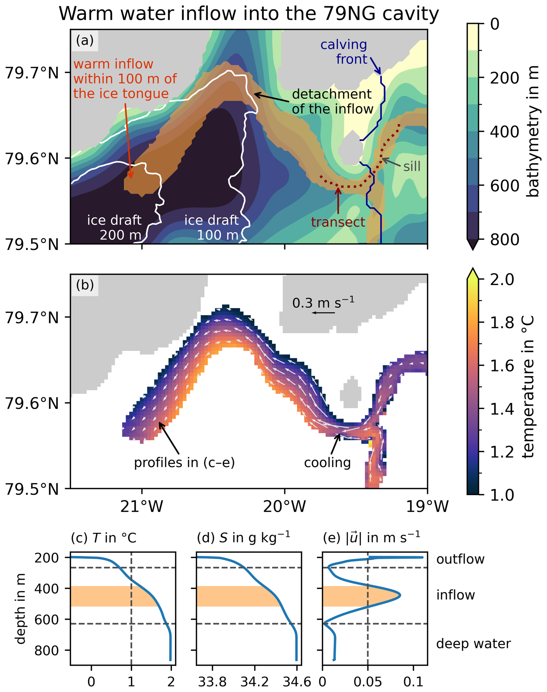
Figure 5 (a) Path of warm AIW flowing into the 79NG cavity (orange overlay) and (b) its vertically averaged velocity (little arrows) and temperature (color shading). (c–e) Vertical profiles of temperature, salinity and speed at the location marked in (b). Orange shadings in (c)–(e) highlight the part of the water column satisfying the criteria used in (a)–(b) with dashed vertical lines marking the thresholds at T=1 °C in (c) and $\left|u\right|=\mathrm{0.05}\mathrm{m}{\mathrm{s}}^{-\mathrm{1}}$ in (e). Dashed horizontal lines in (c)–(e) mark the velocity minima with water in the top layer flowing outward/eastward, including the melt water plume, in the middle layer flowing southwestward, and in the deep layer flowing northeastward with very low velocities. The dotted line in (a) marks the transect passing over the sill shown in Fig. 6.

3.4.2 Vertical structure and hydraulic control of the inflow

As AIW flows down into the cavity, its temperature reduces (see annotation in Fig. 5b). To understand why, we analyze the vertical structure of the inflow along the deepest transect (“thalweg”) passing over the sill (dotted line in Fig. 5a). This is shown in Fig. 6a–e; vertically averaged properties of the inflow computed with the method described in Sect. 2.4 are shown in Fig. 6f–i.

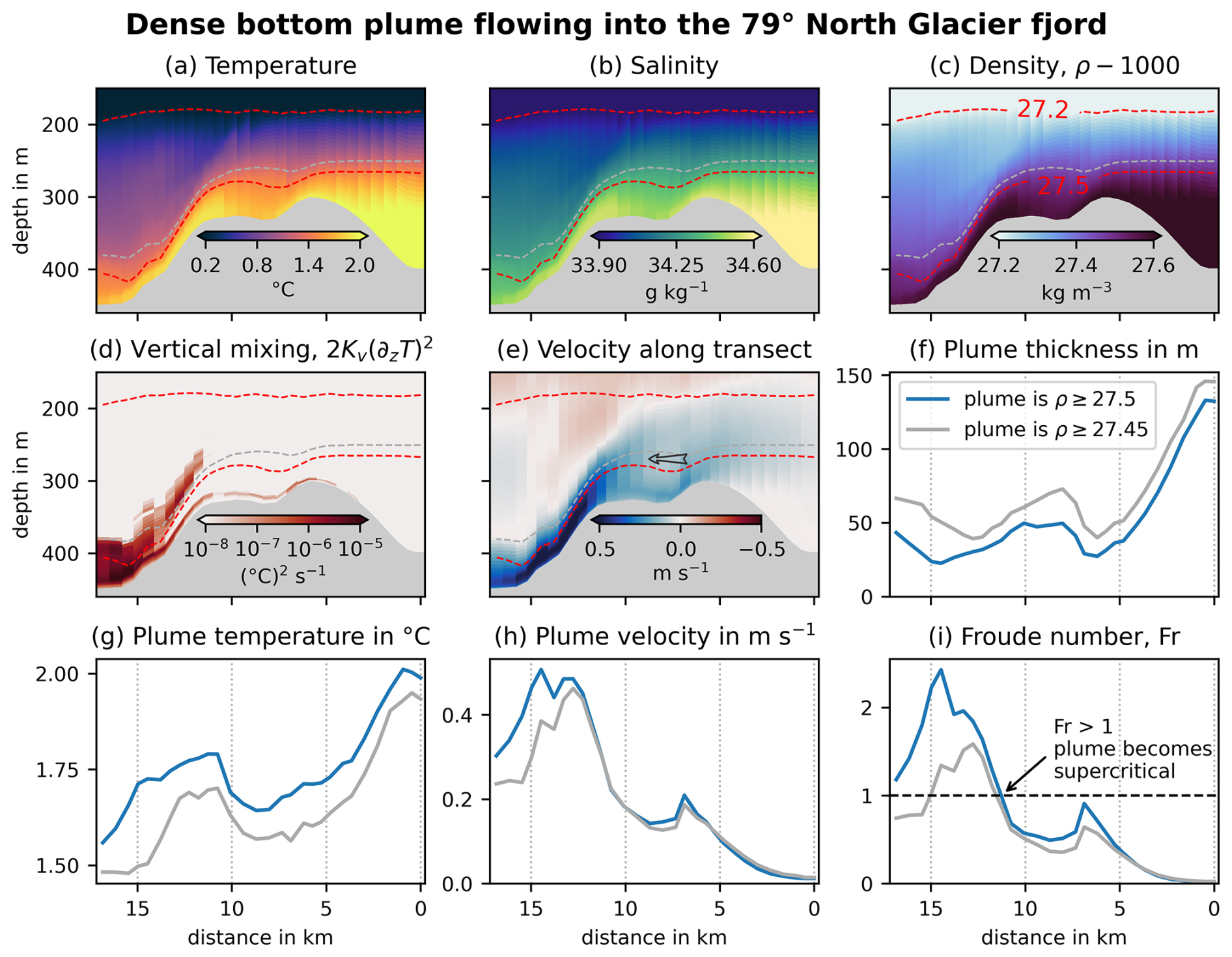
Figure 6 Properties of the inflow into the 79NG fjord along the transect marked in Fig. 5a. Panels (a)–(e) show vertical profiles of temperature (a), salinity (b), density anomaly (c), vertical turbulent mixing of temperature on a log scale (d), and flow velocity in the along-transect direction (e); red dashed lines mark the 27.2- and 27.5-isopycnals used to define the layers of ambient and plume water, see Sect. 2.4. Blue graphs in panels (f)–(i) show bulk properties of the plume: plume thickness (f), vertically averaged temperature (g), vertically averaged velocity (h), and Froude number (i). The sensitivity of the plume properties to the chosen plume interface is shown in gray, corresponding to the 27.45-isopycnal marked as gray dashed lines in panels (a)–(e). The x-axes of all panels show distance along the transect in the direction of the inflow, which is from right to left. Accordingly, positive velocities are also from right to left, as indicated by the arrow in (e). The sawtooth-like pattern visible in the first row is a visual artifact, because each grid cell is colored according to the value at the cell center, but model layers are tilted over sloping topography, resulting in visible differences between adjacent cells.

The warmest and saltiest waters are held back by the sill (Fig. 6a–b) and only the part of AIW above the sill crest passes over it. Consequentially, the vertically averaged temperature between the 27.5 kg m⁻³-isopycnal and the seafloor drops as the inflow approaches the sill (Fig. 6g). On the sill, the inflow becomes bottom-attached (Fig. 6e), so it can be considered a dense bottom plume. The plume is relatively well-mixed compared to the stratified ambient water above (Fig. 6a–c). Downstream of the sill, the inflow warms, as it merges with the inflow coming from the south (see Fig. 5). As the plume reaches the steep slope into the cavity, it accelerates due to gravity and reaches peak velocities of about 0.5 m s⁻¹ (Fig. 6e, h; note that this is the along-transect velocity, whereas the previous Sect. 3.4.1 mentions the magnitude of the horizontal velocity vector). Due to the acceleration, the plume becomes thinner (Fig. 6f). The shear between the fast plume on the sloping bottom and the almost stagnant ambient water above (Fig. 6e) increases turbulence. This leads to a strong increase (at least three orders of magnitude) of vertical temperature mixing at the interface between plume and ambient water (Fig. 6d). The mixing entrains ambient water into the plume, which cools the inflow (Fig. 6g). As the plume reaches the end of the slope, it slows down, increases its thickness, and cools down further due to mixing with the colder ambient water (Fig. 6a, d–h).

The described behavior of the plume on the slope is typical for a transition from subcritical to supercritical flow, and back to subcriticality at the end of the slope. This can be confirmed by computing the Froude number of the plume, using the method described in Sect. 2.4. The Froude number becomes larger than one (Fr>1) as the plume reaches the downward slope (Fig. 6i), showing that the initially subcritical inflow becomes supercritical as it enters the cavity. The gravity current flowing down is thus faster than gravity waves traveling upward on the plume interface, so these waves cannot bring any information out of the cavity. Consequently, the modeled AIW inflow is hydraulically controlled by the sill, in agreement with field observations (Schaffer et al., 2020; McPherson et al., 2024). The implications of this are further discussed in Sect. 4.1.

For the computation of the Froude number, we defined the plume as the water below a chosen isopycnal, and the ambient water as the water between the plume and a second isopycnal (Sect. 2.4). This method was previously used to analyze the inflow at 79NG from measurements, obtaining results similar to ours (Schaffer et al., 2020). We chose 27.5 and 27.2 kg m⁻³ as the two isopycnals and verified that the transition from subcritical to supercritical flow on the slope does not depend on this choice; the same result can also be obtained if the isopycnal choices are varied by ±0.05 or $\pm \mathrm{0.1}\mathrm{kg}{\mathrm{m}}^{-\mathrm{3}}$. The sensitivity of the plume properties to the chosen isopycnal can be estimated from the gray graphs in Fig. 6f–i, showing the plume properties for 27.45 kg m⁻³ as its interface: The plume would be thicker (Fig. 6f) and include more water of lower temperatures (Fig. 6g) and velocities (Fig. 6h). Importantly, the plume becomes supercritical at about the same location (Fig. 6i). However, note that at the end of the transect, the 27.45-isopycnal lies almost outside the inflow, whereas 27.5 stays within the inflow over the whole transect (Fig. 6e).

Any isopycnal should only be considered as an approximation of the plume interface for a particular transect of limited extent. The reason is that the plume density reduces through entrainment of ambient water, meaning that the isopycnals move downward within the plume. Therefore, a fixed isopycnal can be in different dynamic regimes of the plume at the beginning and the end of the transect. Nevertheless, Fig. 6a–e show that the chosen isopycnals follow quite well the shape of the plume.

3.5 Exchange flow and overturning circulation

The inflowing AIW plume and the outflowing meltwater plumes constitute together an estuarine exchange flow, i.e., a zonal overturning circulation in the 79NG fjord. Since the stratification in estuaries is primarily set by salinity, the exchange flow is commonly analyzed in salinity coordinates, by transforming the vertical coordinate from depth to salinity (Burchard et al., 2025). The persistent temperature stratification at 79NG allows doing the same analysis also in temperature coordinates. For the mathematical details of the exchange flow analysis presented in this section, see Sect. 2.5 and 2.6 above.

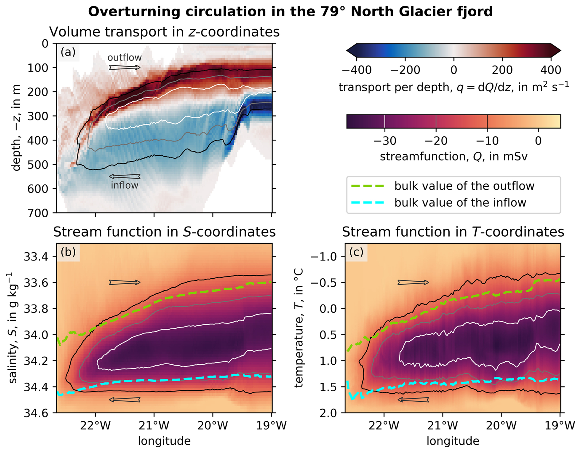
Figure 7 Zonal overturning circulation in the 79NG fjord in z-, S-, and T-coordinates. Panel (a) shows the volume transport per meter depth integrated across the fjord, with a westward propagating inflow (blue) below an eastward propagating outflow (red). Panels (b) and (c) show the overturning stream function with a vertical coordinate of salinity and temperature, respectively; dashed lines are the bulk salinities/temperatures of the in- and outflow. Note that the y-axes of all three panels increase downward to have the inflow below the outflow, as it is in reality. Thin contours in all panels mark the streamlines for $Q=-\mathrm{10}$, −20, −30 mSv.

The zonal velocity, meridionally integrated across the fjord at each depth (−z), shows an inflow through the fjord mouth coming from the east below 200 m depth (Fig. 7a). The inflow passes over the 325 m-deep sill near 19.5° W (Schaffer et al., 2020) and flows down into the cavity to about 500 m depth. Downstream of the sill, the inflow is more spread out vertically. It propagates west toward the grounding line and moves down to about 625 m, the maximum depth of the grounding line.

Near the grounding line, the outflow going eastward above the inflow shows transport maxima at several depths (Fig. 7a). These maxima correspond to the different subglacial meltwater plumes (Sect. 3.3). They start at about 500 m depth and intensify as the plumes flow eastward and upward along the ice tongue. The outflow leaves the cavity between 70 and 200 m below sea level, with maximum volume transport at about 130 m depth, consistent with observations in front of 79NG (Schaffer et al., 2020; Huhn et al., 2021). The glacier tongue near the calving front reaches only 50 to 80 m deep, so the outflow is at greater depth than the ice base.

In salinity coordinates (Fig. 7b) as well as in temperature coordinates (Fig. 7c), the circulation appears mostly as a 2-layer system with an inflow at higher salinities/temperatures and an outflow at lower salinities/temperatures. The streamlines are more closely spaced in the inflow than in the outflow, showing that the inflow occurs over shorter salinity and temperature ranges than the outflow (Fig. 7b, c), despite the inflow covering more depths in the central cavity than the outflows (Fig. 7a). The inflow is thus mostly AIW with temperatures above 1 °C and salinities above 34.2 g kg⁻¹, while the outflow consists of different mixtures of AIW, meltwater and subglacial discharge. The bulk temperature and the bulk salinity of the inflow (computed with Eq. 11) decrease slightly as the inflow passes over the sill (dashed cyan graph in Fig. 7b, c), showing again that not all the warm and salty AIW can enter the cavity. Regarding the outflow, its bulk values decrease eastward, from about 34.0 g kg⁻¹ and +0.8 °C at the grounding line to 33.6 g kg⁻¹ and −0.5 °C at the calving front. This is due to two effects. Firstly, the outflowing plume accumulates more and more meltwater as it flows to the east, making it colder and fresher. Secondly, the eastward flowing plume rises along the ice tongue, passing through the stably stratified water in the cavity. Therefore, the ambient water that is entrained into the plume becomes lighter toward the east (Mohammadi-Aragh et al., 2025).

The outflow at the fjord mouth of Q_out=35.7 mSv is larger than the inflow of $\left|Q_{\mathrm{in}}\right|=\mathrm{35.0}\mathrm{mSv}$, where the difference of 0.7 mSv is explained to 90 % by meltwater, Q_melt=0.638 mSv (Sect. 3.2), and to 10 % by subglacial discharge, Q_runoff=0.070 mSv (Sect. 2.3). The total freshwater flux leaving the cavity, Q_melt+Q_runoff, contributes 2 % to the cavity overturning $\left|Q_{\mathrm{in}}\right|$, and the mixing completeness, $-Q_{\mathrm{in}}/Q_{\mathrm{out}}$ (MacCready et al., 2018; Burchard et al., 2019), is 98 %, meaning that most of the water volume in the outflow originates from inflowing AIW. The other 2 % of the outflowing water volume are freshwater from ocean-driven melting and subglacial runoff, which are mixed by entrainment of AIW to almost ocean salinity before leaving the 79NG fjord. These results agree with mooring data from 2016/2017 within the measurement uncertainties, which gave an overturning strength of (46±11) mSv and a contribution of 1.4 % from the total freshwater flux (Schaffer et al., 2020). The overturning strength is more than 5-times larger than the barotropic flow across the calving front (Sect. 3.1), showing that the cavity circulation is strongly baroclinic and three-dimensional.

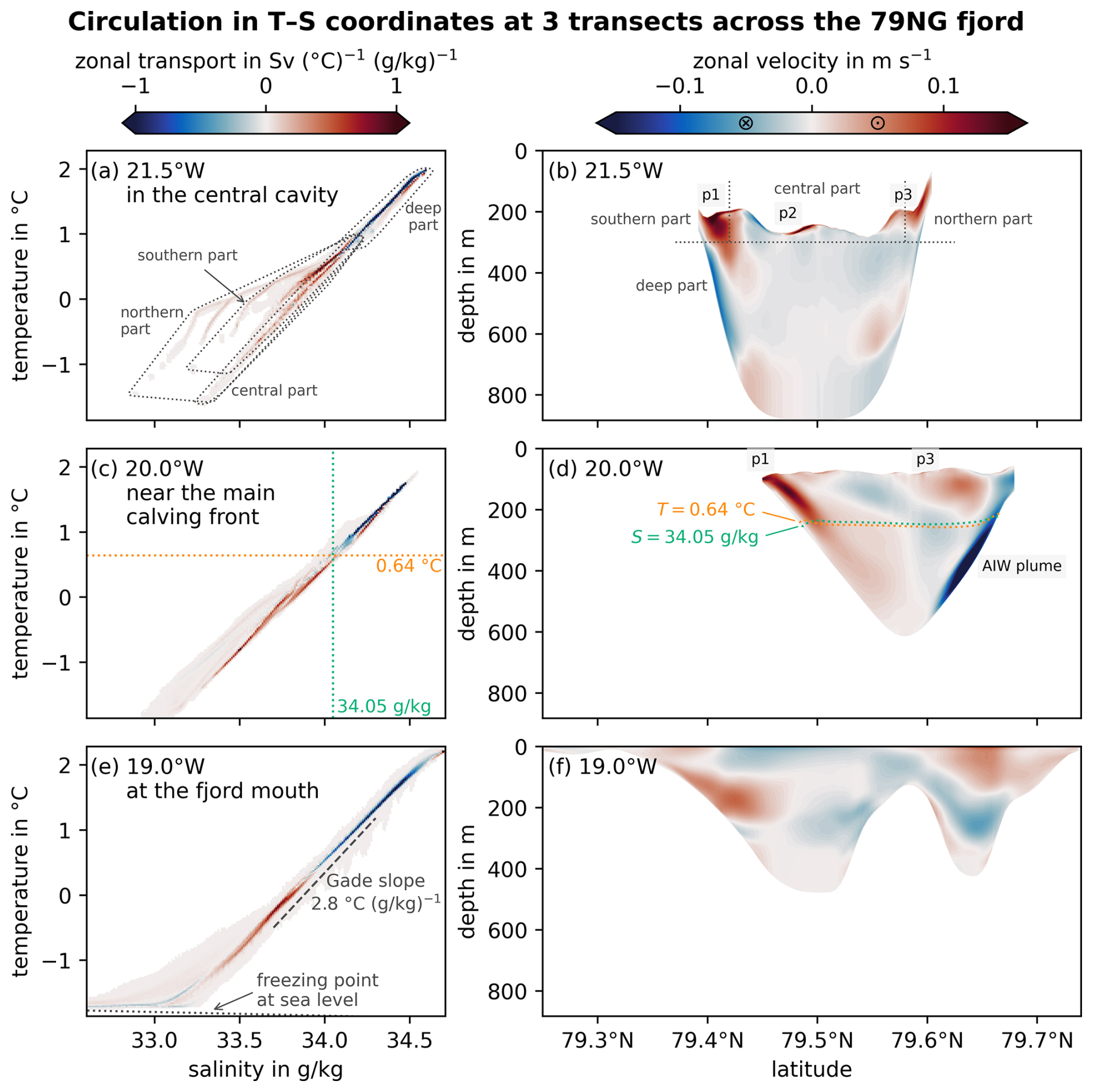
Figure 8 Overturning circulation in the 79NG fjord in temperature–salinity coordinates at three meridional transects: in the central cavity (a, b) and near the main calving front, inside (c, d) and outside (e, f) the cavity. The left column shows the zonal volume transport binned in temperature- and salinity-classes, the right column shows the corresponding zonal velocities in physical coordinates with positive velocities in the out-of-screen direction. The parts of the T–S diagram annotated in (a) correspond approximately to the areas marked in (b). The dividing salinity and temperature marked in (c) correspond to the isohaline and isotherm drawn in (d). The dotted line in (e) shows the freezing temperature at sea level pressure; note that lower temperatures can exist under the ice (e.g., in panel c) due to higher pressure. The labels p1–p3 mark the subglacial plumes annotated in Fig. 4.

3.6 Structure of the plumes in temperature–salinity space

To analyze the plume properties, we map the zonal transport in temperature–salinity (T–S) space (see Sect. 2.5), and find that the strongest exchange flow in the 79NG cavity falls on a straight T–S line (Fig. 8, left column). Generally, a straight line in T–S space is referred to as a mixing line, as it is the effect of turbulent mixing between two water masses (Ferrari and Polzin, 2005). In a glacier cavity, the lighter water mass is basal meltwater and the slope of the meltwater mixing line (or Gade line) can be computed analytically from the properties of the ice and the ambient water (Gade, 1979; Jenkins, 1999; Straneo and Cenedese, 2015). At 79NG, the ambient water mass is AIW and the resulting Gade slope is about 2.8 $\mathrm{°}\mathrm{C}(\mathrm{g}/\mathrm{kg}{)}^{-\mathrm{1}}$, consistent with our model results (Fig. 8e). Deviations from the straight line are due to the influence of other water masses, in particular subglacial discharge and Polar Water offshore the calving front (Huhn et al., 2021).

Near the grounding line, mixing with subglacial discharge creates outflows of lower salinities than the mixing line (Fig. 8a; Straneo and Cenedese, 2015; Hewitt, 2020). These are parts of the southern and northern subglacial plumes (p1 and p3, see Sect. 3.3). Since the northern plume starts at the grounding line (Fig. 4a), the subglacial discharge directly influences its properties. This can explain why it has the lowest salinities, but note the discussion on subglacial discharge in Sect. 4.5.1. Further away from the grounding line, the influence of subglacial discharge on the T–S properties of the exchange flow is reduced, but still visible in deviations from the Gade line toward lower salinities (Fig. 8c). This looks similar to CTD profiles taken directly in front of the 79NG ice tongue (Huhn et al., 2021). Apart from the northern and southern plumes, all other water volumes (and transports) in the cavity lie on the meltwater mixing line, in particular the (primarily outflowing) water masses below the central part of the ice tongue, and the (primarily inflowing) water below 300 m depth (Fig. 8a, b). Note that the divisions marked in panels (a) and (b) of Fig. 8 are only meant as an orientation. Both panels show data temporally averaged in their respective coordinate systems, so there is no one-to-one correspondence between a point in T–S space and a point in physical space.

Comparing a transect landward of the sill (Fig. 8c, d) with a transect on its seaward side (Fig. 8e, f), we see again the effect of the sill in controlling the warm water inflow. The AIW inflow (shown in blue) contains water with temperatures above 2 °C and salinities above 34.5 g kg⁻¹ before (Fig. 8e), but not behind the sill (Fig. 8c), so this warm and salty water seems to be held back by the sill. Both inflow and outflow are mostly bottom-attached and have the land on their right-hand side, indicating geostrophically balanced flow (Fig. 8d, f). Outside the cavity, the cold water mass with salinities well below 33 g kg⁻¹ almost at the freezing point (Fig. 8e) corresponds to Polar Water near the sea level (Huhn et al., 2021). This water mass generally does not enter the cavity, as it is shallower than the ice base.

4 Discussion

4.1 Hydraulic control of the inflowing plume

Our simulation shows that the sill at the fjord entrance has two effects on the inflow of warm and salty AIW into the 79NG cavity. On the one hand, the sill is a physical barrier that limits the inflowing AIW volume and hinders dense water from entering the cavity (Figs. 6a–c, 7, 8c, e). On the other hand, the sill hydraulically controls the inflow, so that the plume becomes supercritical on the downstream slope (Fig. 6i). In consequence, vertical mixing across the plume interface increases strongly (Fig. 6d). The resulting mixing with ambient water cools the inflow, such that less heat is brought into the deep part of the cavity, where the inflow comes near the ice (Fig. 5a, b). Thereby, the hydraulic control reduces ocean-driven basal melting (Nilsson et al., 2023; Wiskandt et al., 2025b), which seems to be a reason why 79NG is one of the few glaciers around Greenland still having a floating tongue.

These results are in line with previous observational (Schaffer et al., 2020) and modeling (Wekerle et al., 2024) studies at 79NG, which identified the role of the sill for constraining inflow volume and heat supply. Furthermore, Nilsson et al. (2023) used a conceptual 2-layer model to explain how hydraulic control increases mixing in the inflow and thereby reduces the thermal forcing at the base of the glacier, compared to cases in which a sill is absent or too shallow to control the inflow. Building on these results, Wiskandt et al. (2025b) studied the effect of the sill for several different sill depths and subglacial discharges in a two-dimensional MITgcm fjord model. The here-presented three-dimensional GETM setup now enables us to resolve these processes in a realistic setting. In particular, the state-of-the-art turbulence closure with GOTM (Burchard et al., 1999; Umlauf and Burchard, 2005) used in our model shows the increase of turbulent mixing due to the hydraulic control, which results in the reduction of heat supply to the glacier base.

4.2 Dynamics of the outflowing plumes

The subglacial plume flowing along the ice base is the driver of basal melting and transports meltwater out of the fjord toward the open ocean (Hewitt, 2020). Our fjord model shows that there is not one, but there are several plumes flowing along different parts of the ice tongue. We classified them as three different plumes in the south, north and center of the ice tongue. The southern plume is the most intense (Fig. 4) and corresponds to the highest melt rates (Fig. 3a). The northern plume contains the freshest water mass (Fig. 8a), presumably due to subglacial discharge (see also Sect. 4.5.1). The central plume is different from the other two, as it is confined to the upper few meters just below the ice and does not continue along the whole ice tongue, but instead merges with the southern plume (Fig. 4a).

The path of all three plumes is determined by the ice topography and the Coriolis effect. They flow primarily in channels at the ice-shelf base and are most intense along the side walls of the channels (Fig. 4c). This is the effect of the Coriolis force, deflecting the plumes to the right (in the flow direction). Accordingly, the highest melt rates are not found in the center of the basal channels, but along their right-hand side in flow direction (Fig. 3a), resulting in an asymmetric channel geometry (see Fig. 4c–e; Sergienko, 2013; Hewitt, 2020). This is analogous to the situation below Antarctic ice shelves, where the plume is deflected to the left and causes higher melt rates on the left side of ice-shelf channels (Alley et al., 2016).

Using a coupled model to simulate ice shelf evolution, Sergienko (2013) showed that basal channels form due to the melting caused by the subglacial meltwater plume. In our simulation, the central plume flows initially in the along-fjord direction, but then turns and reverses (Fig. 4a). The size of these turns is approximately equal to the Rossby deformation radius, i.e., determined by the Coriolis effect. This seems to indicate that the subglacial plume does not only create channels, but might also be responsible for the cone-shaped features in the 79NG ice topography. However, this cannot be said with certainty yet, since our model does not compute the ice shelf evolution happening on longer time scales (Alley et al., 2016; Hewitt, 2020), but only simulates the oceanic flow and ice melting in response to the given topography.

Mohammadi-Aragh et al. (2025) showed with a two-dimensional (x–y) plume model of 79NG that the simulation of the meltwater plume depends strongly on the representation of the ice base, with important implications on the melt rate estimation. If the employed ice topography is smooth, the flow spreads out and the melted area broadens; in contrast, when the ice is channelized, the melt pattern is more focused and spatially heterogeneous (Mohammadi-Aragh et al., 2025). Our computed melt distribution (Fig. 3a) lies between the smooth and channelized experiments of Mohammadi-Aragh et al. (2025). Thus, it is possible that more than three meltwater plumes would appear if our simulation used a finer horizontal grid spacing, resolving more basal channels. On the other hand, models using the smooth ice topography of RTopo-2.0.4 (Schaffer et al., 2019) show only one plume below the 79NG tongue (Wekerle et al., 2024), since this dataset lacks most basal channels.

While the subglacial meltwater plume is initially at the ice base, we see in our simulation that it can detach and flow in a distance from the ice. In a two-dimensional (x–z) simulation of an idealized 79NG fjord, Reinert et al. (2023) showed that the plume detaches from the ice because it reaches neutral buoyancy. It may even overshoot its neutral level, before it propagates away from the ice. With the more complex topography in our realistic simulation, the southern and northern plumes may (partly) detach from and reattach to the ice a number of times (Fig. 4). When propagating out of the cavity below the calving fronts, both plumes are detached from the ice tongue and transport the meltwater out at depth (Fig. 7a), as seen in observational data (Huhn et al., 2021; von Albedyll et al., 2021; Schaffer et al., 2020).

4.3 Importance of three-dimensional effects

The overturning circulation presented in Sect. 3.5 is similar to the 2D-vertical model of the 79NG fjord by Reinert et al. (2023), but with two noteworthy differences. First, the maximum strength of the overturning stream function, Q, is with 36 mSv clearly weaker in 3D than in 2D, where its maximum is over 80 mSv in absolute value. The reason is that in a 2D setup without cross-fjord resolution, the sill at the fjord entrance is as wide as the fjord, allowing for a much greater volume to pass over it, while in the here-presented realistic 3D model, the sill is only a few kilometers wide and allows much less water volume to flow into the cavity.

Second, the inflow and particularly the outflow are much more spread out vertically in 3D than in 2D, due to the more complex topography in 3D: The subglacial meltwater plumes covering parts of the ice tongue are at multiple depth levels in each meridional slice of the 3D fjord (Figs. 4 and 7), but this cannot be represented in a 2D-vertical model. Furthermore, there is no Coriolis force deflecting the flow in the two-dimensional model by Reinert et al. (2023). The Coriolis effect appears in idealized three-dimensional models (Wiskandt et al., 2025a), enhancing melt in the south and reducing melt in the north of the cavity. However, idealized topographies are not sufficient to represent the details of melt distribution, see the comparison between idealized and realistic 3D models by Kanzow et al. (2025). Therefore, while idealized simulations get the principal dynamics in the 79NG cavity right, there are important features of the circulation that only appear in a three-dimensional model with realistic topography resolved on a sufficiently fine grid.

4.4 Advantages and disadvantages of adaptive vertical coordinates

Our model uses adaptive vertical coordinates, while earlier modeling studies of glacier fjords often employed z-coordinates (Wiskandt et al., 2025a, b; Wekerle et al., 2024). For plumes flowing over sloping topography, z-coordinate models generally have larger effective vertical diffusivities due to their staircase manner of resolving sills, which makes gravity currents dissipate too fast, even with high vertical resolutions. This problem does not occur in topography-following coordinates, as they almost eliminate flow across layers for topography-following currents. Numerical mixing is further reduced with stratification-aware vertical coordinates, like those used in GETM (Hofmeister et al., 2010; Reinert et al., 2023). The effect is that the inflowing plume stays narrow and focused in our simulation (Fig. 6) and does not diffuse much through spurious mixing as it flows down the slope, allowing the water to propagate further into the cavity. The same applies to the meltwater plumes, which are well-resolved by the adaptive vertical coordinates used in our model (Fig. 4). This close-to-reality depiction of the in- and outflowing currents in our simulation is important for an accurate representation of ocean-driven basal melting (Reinert et al., 2023; Burchard et al., 2022), which is necessary to analyze glacier stability. Nevertheless, it is worth noting that also models with z-coordinates generally compute realistic melt rates (Kanzow et al., 2025), presumably because the effects of unresolved processes can cancel each other to some extent. A possible explanation can be that without a well-resolved meltwater plume, the water at the ice base is too warm, but the friction at the ice–ocean interface is too low, which may result in a melt rate similar to that induced by a colder plume exerting more friction.

While the simulation of the plumes works well in adaptive vertical coordinates, the calving front presents a challenge. This front is almost vertical in reality, which blocks barotropic flow from entering the cavity (Grosfeld et al., 1997; Wåhlin et al., 2020). However, the ice front stretches out over a few grid cells in models with topography-following coordinates like ours, facilitating barotropic flow into the cavity. This does not seem to cause big issues in our simulation, because the barotropic transport across the calving front is low compared to the strength of the baroclinic inflow (Sect. 3.1 and 3.5). But this might change in the presence of wind-driven circulation, when atmospheric forcing is included in the model (see Sect. 4.5.2). On the other hand, barotropic blocking may also be reduced in reality, which can make the sloping front in the model acceptable. Observations in Antarctica showed that melting at the ice front creates a wedge of fresher water, reducing the blocking effect of the vertical wall and allowing currents to enter the cavity more easily (Malyarenko et al., 2019). It is plausible that this wedge appears at 79NG, too, which would further reduce possible issues at the calving front.

4.5 Steps toward a fully realistic fjord model

The model of the 79NG fjord presented here uses realistic topographies for the ice base and the seafloor (Sect. 2.2), combined with stationary forcings (Sect. 2.3): The prescribed conditions at the open ocean boundaries (Fig. 1d–e) and the initial conditions come from a realistic global model averaged over a ten-year period (2011–2020); the subglacial discharge is the one-year average from mooring data (2016/2017). This forcing was used to analyze the steady state circulation in the glacier cavity at present day. Our results, which are generally consistent with observations and previous studies, should thus be seen as a description of the one- or multi-year average situation in the fjord. The temporal variability of the circulation is, however, not represented in our model and would require time-resolved forcings, as explained in the following two subsections.

4.5.1 Temporal and spatial variability of subglacial discharge

Subglacial discharge is prescribed in our setup as a constant freshwater input of 0.07 mSv across the grounding line, corresponding to 2.2 km³ yr⁻¹ (value given in cubic kilometers per year for comparison with the following references). In reality, this transport varies strongly on interannual and seasonal timescales (Hewitt, 2020). Narkevic et al. (2023) computed the yearly runoff at 79NG from the 1970s to today; they found annual averages between 0.1 and 1 km³ yr⁻¹. However, Wekerle et al. (2024) found an interannual variability of 79NG discharge from 2 to 10 km³ yr⁻¹, using data by Mankoff et al. (2020a) for the same time period. While both time series have similar interannual variabilities, their values differ by a factor of 10. This difference presumably reflects the definition of the catchment area for 79NG runoff and shows that significant uncertainty exists in subglacial discharge. The observation-based value (Schaffer et al., 2020) used in our setup lies in between those two time series. Regarding the seasonal variability, Wekerle et al. (2024) showed that the discharge at 79NG is essentially zero from September to May, increases in June, reaches its maximum in July and decreases in August. The peak discharge in mid-July is with almost 70 km³ yr⁻¹ about an order of magnitude larger than the annual average. The 2.2 km³ yr⁻¹ runoff in our model is thus more similar to the nine months of no discharge than to the three summer months.

Previous modeling studies have investigated the effect of subglacial discharge variations at 79NG and give us an idea of how our results would change under variable runoff. Ocean-driven melting increases with the square root of the discharge (Reinert et al., 2023; Wekerle et al., 2024) when the melt rate is averaged over the whole ice tongue. Near the grounding line, the melt rate increases even more (Reinert et al., 2023), whereas the melt rate closer to the calving front is almost unaffected by the discharge (Mohammadi-Aragh et al., 2025). Under stronger runoff and consequently increased basal melting, the water in the cavity is colder and fresher, the plumes are thicker and faster, and the exchange flow between fjord and open ocean is enhanced (Reinert et al., 2023). In contrast, during low-discharge periods, the AIW inflow may be slower and propagate less deep into the cavity due to the reduced freshwater input at depth (Reinert et al., 2023). The effects of stronger melting and an accelerating meltwater plume appear almost immediately when the discharge increases in summer (Wekerle et al., 2024).

During summer months, when subglacial discharge is present, its spatial distribution is important. While the discharge is uniformly distributed along the grounding line in our model (Sect. 2.3), it is more likely to enter the cavity through discrete channels in reality (Hewitt, 2020). Narkevic et al. (2023) showed that these channels may change over time, with three main subglacial runoff outlets and a varying number of smaller outlets at the 79NG grounding line. With channelized discharge, melting is more localized within those channels, and high melt rates extend further along them (Mohammadi-Aragh et al., 2025). This is different from the more uniform distribution of high melt rates near the grounding line in our simulation (Fig. 3a). Mohammadi-Aragh et al. (2025) also showed that discharge through discrete channels may increase the overall melt rate by 20 %–30 % compared to uniformly distributed discharge; however, these numbers are for an intense runoff of $\mathrm{4.8}\mathrm{mSv}\approx \mathrm{150}{\mathrm{km}}^{\mathrm{3}}{\mathrm{yr}}^{-\mathrm{1}}$, almost 70 times that of our setup. Therefore, we expect the impact of channelized discharge to be less strong in our simulation.

4.5.2 Influence of oceanic and atmospheric forcing

Another key source of variability is the oceanic forcing applied at the open boundaries of our fjord model. While a climatological ocean forcing is used in our setup, recent studies highlight significant interannual variability in AIW temperatures. Wekerle et al. (2024) documented AIW temperature fluctuations between 1 °C and more than 2 °C, with a warming trend from 1970 to 2021 of 0.19 °C per decade on average. Similarly, McPherson et al. (2024) observed strong year-to-year variations in the maximum water temperatures from mooring measurements (2016–2021), including a notable decline of AIW temperatures by 0.65 °C between 2018 and 2021. This cooling is associated with a thinning of the AIW layer and a reduced heat transport into the cavity (McPherson et al., 2024). On the other hand, periods of increasing AIW interface height led to more heat transport and melting (Schaffer et al., 2020). Consequently, we expect the inflow and thus the melt rate and overturning strength in our model to be temporally variable if time-dependent ocean conditions are applied.

This inflow variability can explain the presence of the deep water mass in the cavity mentioned in Sect. 3.4.1. In our simulation, the water below the maximum ice draft (625 m) is essentially stagnant (Fig. 5e) and contributes little to the cavity overturning (Fig. 7a), as there is no freshwater source at that depth (see also Reinert et al., 2023). The properties of this water mass are set primarily at initialization with data from a realistic global model (Sect. 2.3). In non-stationary simulations, periods of increased AIW transport can allow the inflow to propagate further down and lead to the renewal of the water in the deep cavity below the grounding line depth.

A fully realistic model of the 79NG fjord should also include atmospheric forcing, which is not considered in our current setup. As the glacier cavity is isolated from the atmosphere by the floating ice tongue, the atmosphere can only have a direct effect on the part of the fjord offshore the ice front. However, the area around 79NG is covered with land-fast sea ice, the Norske Øer Ice Barrier (Sneed and Hamilton, 2016), during most of the year (Schaffer et al., 2020). Thus, the inclusion of atmospheric forcing would also require coupling with a sea ice model, since fast ice acts as a rigid cap between atmosphere and ocean (Sneed and Hamilton, 2016). In recent decades, breakups of the ice barrier in summer have become more frequent (Sneed and Hamilton, 2016), making direct ocean–atmosphere interactions in the 79NG fjord possible. The prevailing winds at 79NG are katabatic (Turton et al., 2019), i.e., downslope from the glacier to the ocean. During ice-free times, these winds can drive transports in the upper ocean layer with associated up- or downwelling. However, due to the strong near-surface stratification of Polar Water, it is unlikely that these wind effects reach far enough down to affect the inflow of AIW (Brown et al., 2020). In an idealized modeling study, Carroll et al. (2017) found that the wind effect in a fjord with comparable stratification (Polar Water above Atlantic Water) is limited to the upper 50 m of the water column. Consequently, we can assume the exchange flow at 79NG below the calving front draft (50–80 m) to be largely unaffected by atmospheric forcing in the fjord.

Nevertheless, atmospheric processes outside the fjord do have an impact on 79NG. Firstly, subglacial discharge originates partly from the surface of the ice sheet, and this surface melt is atmosphere-driven (Kanzow et al., 2025). Secondly, atmospheric processes in the Nordic Seas modify the properties of the Atlantic Water near the sea surface before it subducts below Polar Water in central Fram Strait and becomes the AIW that flows toward the 79NG fjord (von Albedyll et al., 2021; McPherson et al., 2024). These far-field atmospheric influences enter our fjord model indirectly by setting the boundary conditions at the grounding line and in the open ocean.

5 Conclusions

We developed a three-dimensional model of the 79NG fjord to show in detail how the oceanic circulation melts Greenland's largest floating glacier tongue. For the simulation of a typical state at present day, we employed realistic topographies of the ice tongue as well as the seafloor, and used steady, temporally averaged forcing data from a global model. With about 500 m in the horizontal, the grid resolution is sufficiently fine to resolve larger basal channels in the ice, which are typically between 500 m and a few kilometers in width. These channels are the areas where most melting occurs at the floating glacier tongue. The melt rate computed by our model looks qualitatively similar to satellite observations. Also, the total melt volume is consistent with oceanographic measurements, although it lies rather at the higher end of the range estimated from in situ data, likely due to a warm bias in the employed forcing. Furthermore, the strength of the cavity overturning and the depth of the meltwater export are both in line with observations at the fjord entrance.

Our simulation shows that the subglacial plume, melting the 79NG tongue from below, is made up of three separate plumes flowing along different parts of the ice tongue. We mapped the distinct properties of these plumes in physical space as well as in T–S space. The plumes flow primarily from the grounding line toward the calving front along the right flank of basal channels, due to the Coriolis effect. This was expected from observations and previous modeling studies. However, we also saw that the central plume can reverse direction by turning around cone-like structures in the ice topography. The size of these features in the ice is similar to the Rossby deformation radius, which suggests that these cones may be shaped by the subglacial plume itself under the influence of Earth rotation. To confirm this hypothesis, further investigations using a coupled model will be necessary.

The heat supply for melting the floating glacier tongue is provided by an inflow of relatively warm and salty AIW. This inflow is limited by the sill at the fjord entrance through hydraulic control, which strongly enhances mixing with ambient water, thereby cooling the inflow. While these processes have been described previously, our model actually resolves them and shows how the inflowing warm water is distributed in the cavity, bringing the heat close to the ice base. Resolving the transition of the inflow from sub- to supercritical flow requires a high vertical resolution. This is achieved in our model by using adaptive vertical coordinates, which also provide a resolution of about 1 m in the plumes at the ice-shelf base to accurately represent their dynamics.

The findings presented here suggest several directions for future research. First, a coupled ice–ocean model should be used to test the hypothesis that the meltwater plume creates cone-like structures in the floating ice tongue (Sect. 4.2). Second, time-dependent forcing can be used in our fjord model to study seasonal and interannual deviations from the quasi-steady state circulation in the 79NG cavity (Sect. 4.5). Third, global ocean models could be equipped with the adaptive coordinates employed here (Sect. 4.4) to study with high vertical resolution glacier cavities around Greenland and Antarctica.