A nine-year record of slush on the Greenland Ice Sheet

Surface melt on the Greenland Ice Sheet has intensified in recent decades, accelerating mass loss. Slush, i.e., water-saturated snow or firn, is a key component of the ice sheet's surface hydrological system, yet its extent and behaviour remain poorly constrained. We present the first classification of slush across the Greenland Ice Sheet, using Sentinel-2 imagery and a random forest classifier to generate a nine-year dataset spanning 2016–2024. Over this period, slush covered a mean seasonal extent of 2.8 % of the ice sheet (∼ 48 100 km²), ranging from 1.1 % (∼ 18 700 km²) in 2018, the lowest-melt year, to 5.1 % (∼ 88 500 km²) in 2019, the highest-melt year. Slush was most extensive in the southwestern and northern basins and most recurrent in the northern and northeastern basins; across these regions, its distribution was associated with bare ice, low-permeability ice slabs and, potentially, finer-scale firn heterogeneity. Slush was the dominant mapped surface meltwater feature by area: in 2019, its extent was nine times the reported combined area of supraglacial lakes, channels, and water-filled crevasses. The mean elevation of the upper slush limit broadly covaried with slush extent, with both increasing during high-melt years. Slush extent and occurrence were associated with higher snowmelt and lower firn air content, while a first-order upper-bound estimate suggests that additional energy absorption associated with slush could produce a mean melt equivalent of 12.4 Gt yr⁻¹ if fully converted to melt. As the ice sheet warms, slush is likely to play an increasingly important role in the surface hydrological system, and its explicit representation in surface energy-balance and hydrological models is required to better constrain future ice-sheet mass-balance projections.

1 Introduction

The Greenland Ice Sheet (GrIS) has experienced a negative mass balance for several decades, losing ice at a rate of 169 ± 9 Gt yr⁻¹ between 1992 and 2020 (Otosaka et al., 2023). Surface melting and runoff are major contributors to this mass loss, accounting for just over half of the total ice-sheet mass loss between 1992 and 2018 (The IMBIE Team, 2020). Mean summer air temperature on the GrIS increased by ∼ 1.7 °C between 1991 and 2019 (Hanna et al., 2021), contributing to a 21 % increase in surface runoff during 2011–2020 relative to the preceding three decades (Slater et al., 2021; Trusel et al., 2018). Superimposed on this long-term warming trend are increasingly frequent extreme melt events (Bonsoms et al., 2024), which are short-lived episodes of anomalously intense melting typically driven by persistent high-pressure systems (Tedesco and Fettweis, 2020). In response to both long-term warming and the increasing frequency of extreme melt events, supraglacial meltwater features, particularly lakes, have expanded in area and to higher elevations over recent decades (Fan et al., 2025; Leeson et al., 2015; Howat et al., 2013). Between 1985 and 2020, the upper elevation limit of runoff increased by up to 329 m a.s.l. and extended inland into higher-elevation reaches of the percolation zone in some regions (Tedstone and Machguth, 2022; Tedesco, 2007; Fettweis et al., 2011). This inland expansion of melt has been accompanied by reductions in firn air content (FAC), including a 23 ± 16 % decline in the low-accumulation area of the western Greenland percolation zone from 1998–2008 to 2010–2017 (Vandecrux et al., 2019). Enhanced meltwater production and reduced firn storage capacity favour the formation of slush, defined here as water-saturated firn or snow (Cogley et al., 2011).

Slush, first observed during Greenland expeditions in the early twentieth century and formally described by Holmes (1955), forms when vertical drainage is impeded, either because a low-permeability ice layer blocks percolation or because meltwater fills the available pore space, causing the overlying firn or snow to become water-saturated. Holmes (1955) distinguished between surface and subsurface slush. Surface slush, referred to as blue slush, is saturated to the surface and can therefore be detected in optical satellite imagery, whereas subsurface slush, referred to as white slush, is overlain by unsaturated snow and cannot be identified in optical imagery (Greuell and Knap, 2000; Machguth et al., 2022). Once formed, slush promotes the preferential lateral rather than vertical routing of meltwater. This process enhances surface hydrological connectivity, as meltwater flows more readily through slush than through dry snow and firn (Clerx et al., 2022), feeding supraglacial channels and lakes (Holmes, 1955). Slush can act as a precursor to supraglacial channelisation, either by directing excess meltwater into topographic depressions, where channel incision may begin (Chu, 2014; Rippin and Rawlins, 2021), or by facilitating the removal of the previous winter's snow from existing channels (Tedesco et al., 2013). These channels can connect to moulins or crevasses, providing pathways through which meltwater is routed to the ice-sheet bed (Tedesco et al., 2013; Banwell et al., 2013, 2016), thereby influencing basal lubrication and ice dynamics (e.g., de Fleurian et al., 2018; Koziol and Arnold, 2018). Upon refreezing, slush can form new near-surface ice slabs or thicken existing slabs (Tedstone et al., 2025). These multi-metre-thick bodies of refrozen ice can extend over tens of kilometres (Machguth et al., 2016; MacFerrin et al., 2019; Jullien et al., 2025) and, because of their low permeability, restrict vertical meltwater transport and reduce firn storage capacity, thereby enhancing runoff from inland areas (Machguth et al., 2016; Tedstone and Machguth, 2022; Culberg et al., 2024).

Despite its hydrological importance, slush remains largely absent from large-scale meltwater mapping efforts across the GrIS. Only a limited number of studies have attempted to quantify its areal extent or upper elevation limit, either through catchment-scale mapping of its spatial distribution (e.g., Covi, 2022; Rawlins et al., 2023; Glen et al., 2025) or, at larger spatial scales, by identifying the “runoff limit”, defined as the highest elevation at which visibly saturated firn or snow is present in satellite imagery (Greuell and Knap, 2000; Tedstone and Machguth, 2022; Machguth et al., 2022). Recent observations indicate that both the areal and elevational extent of slush vary substantially with inter-annual melt conditions. Within the Watson catchment in southwest Greenland, for example, slush covered a substantially larger area and extended to higher elevations during the extreme melt year of 2019 than during the below-average melt year of 2018 (Glen et al., 2025). Its areal extent increased from 1.6 % of the catchment (∼ 80 km²) in 2018 to 7.6 % (∼ 380 km²) in 2019, while its upper elevation limit increased from below 1500 m a.s.l. to above 1800 m a.s.l. Similarly, long-term satellite analyses indicate an upward migration of the runoff limit across the GrIS: Landsat imagery revealed a 29 % expansion in runoff area between 1985 and 2020 (Tedstone and Machguth, 2022), while MODIS imagery detected slush at elevations approaching 2080 m a.s.l. in western Greenland (Machguth et al., 2022).

Recent findings from Antarctic ice shelves further emphasise the broader importance of slush to polar ice-sheet hydrology and mass balance. Dell et al. (2024) showed that in January (mid-austral summer), slush accounted for 57 % of the mean total surface meltwater area across 57 ice shelves, suggesting that previous meltwater inventories focused primarily on supraglacial lakes and channels may substantially underestimate total surface meltwater area. Dell et al. (2024) also demonstrated that, across five representative ice shelves, adjusting surface albedo in a regional climate model to account for the lower albedo of slush and ponded water increased modelled snowmelt to 2.8 times the original estimate. Explicitly accounting for slush in ice-sheet meltwater budgets and surface energy-balance models is therefore necessary to improve estimates of present-day and future surface melt and runoff.

Here, we adapt a machine learning (ML) workflow developed for Antarctic ice shelves (Dell et al., 2022a, 2024) to classify blue surface slush (henceforth “slush”) across the entire GrIS using Sentinel-2 (S2) imagery in Google Earth Engine (GEE). This represents the first application of ML to map slush on the GrIS, through which we generate an ice-sheet-wide dataset of slush extent spanning nine years (2016–2024). Using these data, we characterise the distribution and persistence of slush across all six drainage basins and examine its spatial and temporal variability, elevational patterns, associations with environmental conditions, and relative importance within the broader GrIS surface meltwater system.

2 Methods and data

To date, the majority of remote-sensing studies of supraglacial meltwater features on the Earth's ice sheets have focused on lakes and channels, which have relatively distinct spectral characteristics and well-defined boundaries. Compared with slush, these features can therefore be mapped with reasonable accuracy using threshold-based methods, such as the Normalised Difference Water Index adapted for ice (NDWI_ice) (e.g., Williamson et al., 2017, 2018; Miles et al., 2017). Slush has diffuse boundaries and a muted blue hue in optical imagery, making it difficult to isolate using standard thresholding techniques. In such approaches, slush is typically either omitted entirely and classified as “non-water” or included within broader “water” classes without being distinguished from lakes or channels, leading to the underestimation or mischaracterisation of its extent (e.g., Rawlins et al., 2023; Yang and Smith, 2012).

Random forest (RF) algorithms (e.g., Dirscherl et al., 2020; Dell et al., 2022a, 2024) and deep-learning methods (e.g., Qayyum et al., 2020; Dunmire et al., 2025) have recently shown promise as alternatives to image thresholding for meltwater classification in both Greenland and Antarctica. For slush specifically, Dell et al. (2022a, 2024) employed a k-means clustering approach to generate training classes from Landsat 8 imagery, which were then used to train an RF classifier to identify slush and supraglacial water bodies on Antarctic ice shelves. However, no study has yet applied such ML classification methods specifically to slush detection on the GrIS.

Here, we classified slush on the GrIS following the approach outlined by Dell et al. (2022a, 2024), with adaptations for its application to the GrIS, as detailed in the following sections and Fig. 1. We retained the general workflow of Dell et al. (2022a, 2024), originally developed for Landsat 8 optical imagery, including k-means clustering for training-data generation, NDWI_ice-based pre-thresholding, and RF classification in GEE (Gorelick et al., 2017). However, we made several adaptations for application to S2 imagery, including adjustments to spectral thresholds to account for sensor differences and the addition of RF hyperparameter optimisation to improve classification performance. All image pre-processing, training-data generation, RF classification, and post-processing were implemented in GEE, with the final binary slush masks exported at a spatial resolution of 100 m (Glen, 2026). We conducted our analysis across all six basins of the GrIS: Southwest (SW), Central West (CW), Northwest (NW), North (NO), Northeast (NE), and Southeast (SE) (Fig. 2; Mouginot and Rignot, 2019).

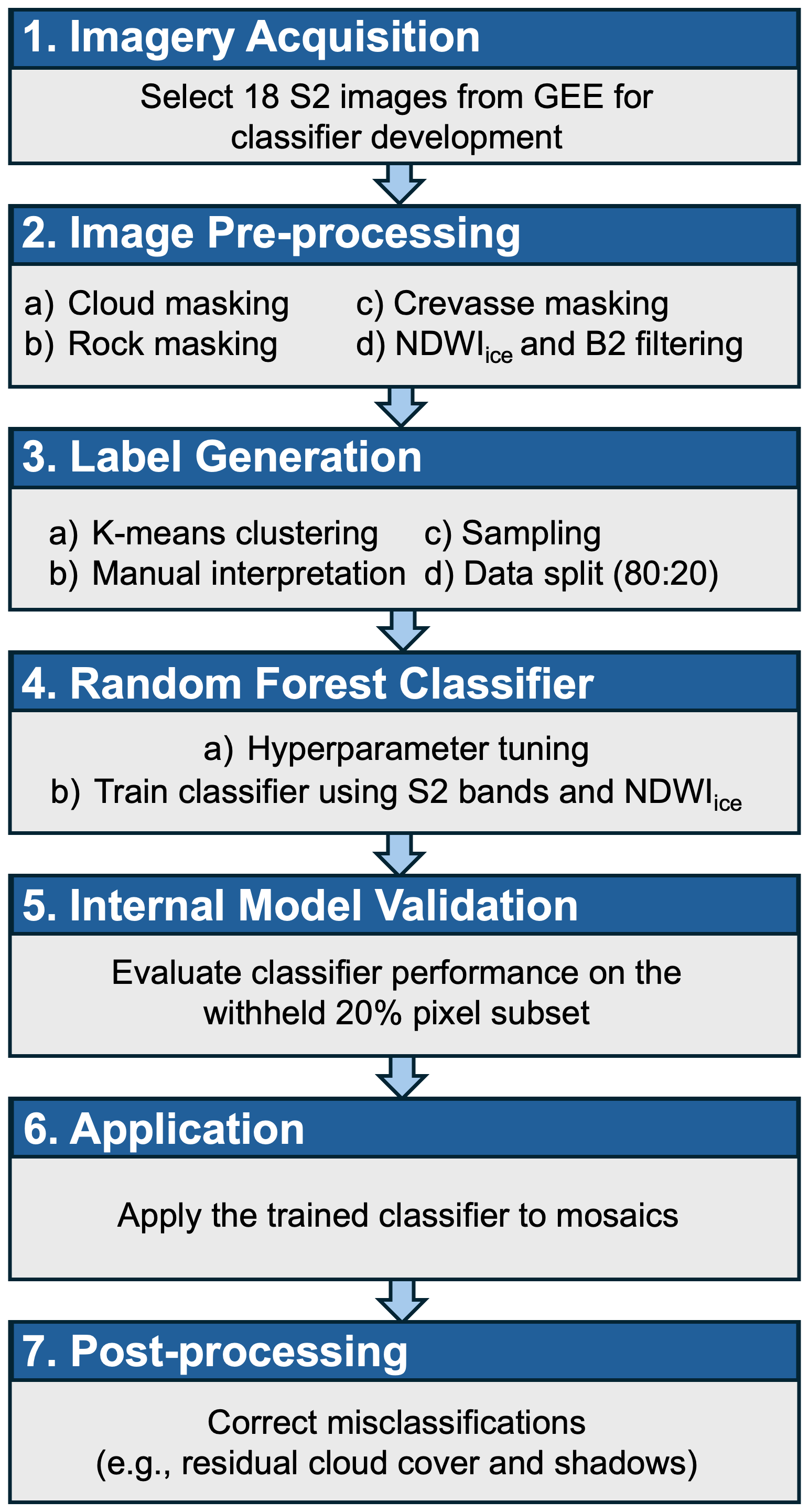
Figure 1 Flowchart of the slush-classification methodology adapted from Dell et al. (2022a, 2024), originally developed for Antarctic ice shelves, for application to the GrIS in this study.

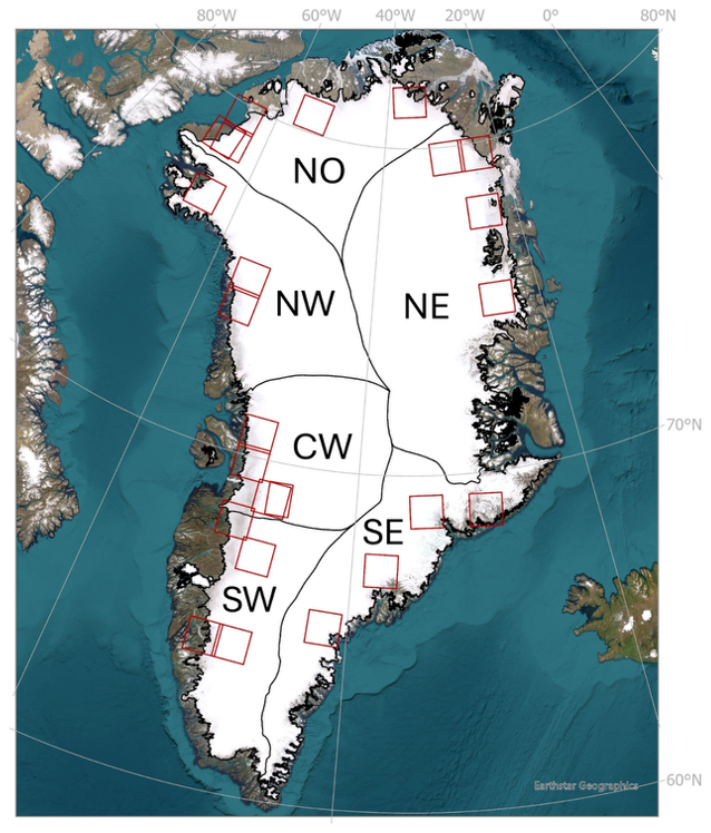
Figure 2 Overview map of the GrIS divided into six drainage basins: SW, CW, NW, NO, NE, and SE (Mouginot and Rignot, 2019). Red boxes indicate the footprints of the 24 S2 images used in this study for classifier development and evaluation: 18 for training and internal validation of the RF classifier and a further 6 for comparison with threshold-based classification methods. Base map source: Esri (2024) Earthstar Geographics | Powered by Esri.

2.1 Data

2.1.1 Sentinel-2 imagery

We acquired and pre-processed Level-1C S2 MultiSpectral Instrument (MSI) imagery from the European Space Agency (ESA) via the GEE data catalogue, processing a total of 329 229 images acquired between May and September from 2016 to 2024. As Level-1C imagery is provided as scaled top-of-atmosphere reflectance, pixel values were divided by 10 000 to scale the reflectance values between 0 and 1 (ESA, 2015). To improve meltwater-feature detection, we restricted the dataset to scenes with a solar elevation angle > 20° (Halberstadt et al., 2020) and cloud cover < 25 %, following filtering approaches commonly used in supraglacial meltwater-feature mapping studies (e.g., Corr et al., 2022; Glen et al., 2025; Tuckett et al., 2025). Although pixel-level cloud masking was subsequently applied, this pre-filter helped reduce residual cloud-shadow artefacts and ensured sufficient clear-sky pixel coverage for compositing. All available MSI bands were used, with GEE dynamically handling differences in native spatial resolution using default nearest-neighbour resampling.

2.1.2 Supporting datasets

We used the 2 m ArcticDEM mosaic (Porter et al., 2023) to provide high-resolution surface topography across the ice sheet. ArcticDEM was used to mask crevassed areas following Chudley et al. (2021) and to characterise the elevation of the upper slush limit. Elevations were sampled at 500 m intervals along the mapped upper slush limit and averaged to calculate its mean elevation.

Firn extent for 2000–2017 was taken from Vandecrux et al. (2019), based on firn-density observations and end-of-summer snowline data. Ice-slab extents were taken from Jullien et al. (2023), who used airborne accumulation-radar data collected across the GrIS between 2002 and 2018 to map spatial variations in ice-slab extent and thickness. We used both their low-end and high-end estimates of slab extent in our analysis. Firn-aquifer extents were taken from Miège et al. (2016), who identified aquifers using NASA Operation IceBridge accumulation-radar data collected during five airborne campaigns between 2010 and 2014. Since these datasets represent different periods, they were used as contextual spatial overlays rather than as strictly contemporaneous representations of conditions during 2016–2024.

Snowfall, snowmelt, and 2 m air temperature data were obtained from the Regional Atmospheric Climate Model RACMO2.3p2 (hereafter “RACMO”; Noël et al., 2019). RACMO is forced by ERA5 and provides monthly snowfall, snowmelt, and 2 m air-temperature fields at a spatial resolution of 5.5 km, statistically downscaled to 1 km (Noël et al., 2018, 2019). FAC was derived from the Institute for Marine and Atmospheric Research–Firn Densification Model (IMAU-FDM), a one-dimensional, semi-empirical model that is also forced by ERA5 and dynamically downscaled using RACMO. IMAU-FDM provides FAC fields at a temporal resolution of 10 d and a spatial resolution of 5.5 km (Brils et al., 2022); because data were available only through 2023, FAC-based analyses covered 2016–2023.

Snowfall, snowmelt, 2 m air temperature, and FAC anomalies were calculated relative to the 1960–1989 monthly climatology, a period during which the ice sheet is assumed to have been approximately in a steady state with climate forcing (Mouginot et al., 2019). Anomalies were calculated for each melt-season month (May–September) and for each year between 2016 and 2024. These anomaly datasets were used to characterise inter-annual variability in snowfall, snowmelt, 2 m air temperature, and FAC during the study period.

2.2 Image pre-processing

2.2.1 Image masking

To mask confounding surface features, we applied a cloud-detection algorithm based on S2-specific thresholds from Glen et al. (2025), following Corr et al. (2022), with a 1 km buffer to account for cloud shadows. Rock outcrops were excluded using a modified Normalised Difference Snow Index approach, as detailed in Glen et al. (2025) following Moussavi et al. (2020), with a 1 km buffer also applied to ensure complete removal. A crevasse mask derived from the 2 m ArcticDEM (Porter et al., 2023) was used to remove crevassed areas and prevent misclassification errors (Chudley et al., 2021). Meltwater features, including slush, were then isolated using an NDWI_ice threshold (Eq. 1), which is a variant of the standard NDWI (McFeeters, 1996). Whereas the standard NDWI, calculated using the green (B3) and near-infrared (B8) bands, is commonly applied in terrestrial environments and, in some cases, to ice-sheet surfaces (e.g., Box and Ski, 2007), NDWI_ice is specifically optimised for ice and firn surfaces and instead uses the blue (B2) and red (B4) bands (Yang and Smith, 2012).

$$\begin{array}{}\text{(1)}& {\mathrm{NDWI}}_{\mathrm{Ice}}={\displaystyle \frac{\mathrm{B}\mathrm{2}-\mathrm{B}\mathrm{4}}{\mathrm{B}\mathrm{2}+\mathrm{B}\mathrm{4}}}\end{array}$$

Whereas Dell et al. (2022a) applied an NDWI_ice threshold > 0.1 to Antarctic ice shelves, we increased this threshold to > 0.12 for Greenland (Yang and Smith, 2012) to account for regional differences in surface albedo and reflectance. Additionally, we applied a blue-band reflectance threshold > 0.03 to filter out shadows cast by rocks, crevasses, and other non-meltwater features (Dirscherl et al., 2020; Corr et al., 2022).

2.2.2 S2 image mosaic creation

For each basin and year from 2016 to 2024, monthly S2 mosaics were generated for May, June, July, August, and September, together with a seasonal mosaic spanning the full May–September period. After image filtering and masking, all available S2 images were combined into mosaics using the qualityMosaic function in GEE, which selects, for each pixel, the observation with the highest NDWI_ice value among overlapping images to capture the strongest potential meltwater signal within a given month or season (Dell et al., 2022a). These monthly and seasonal mosaics were then used as input datasets for the RF classifier (Sect. 2.4). The observation with the highest NDWI_ice value was selected independently for each pixel; therefore, the resulting slush areas represent composite footprints of pixels classified as slush during the corresponding month or season, rather than areas that were necessarily covered by slush simultaneously on a single date.

2.3 Label generation for model training and validation

For each GrIS drainage basin (Fig. 2), we manually selected three S2 images for training and validation, giving a total of 18 images across the six basins (Table S1 in the Supplement). Images were selected from the 2016–2024 melt seasons (1 May–30 September) to capture spectral variability across a range of solar elevation angles (42–75°) and both high- and low-melt conditions. Each image was clipped to the boundary of its corresponding drainage basin (Fig. 2).

Following pre-processing, residual non-meltwater elements, such as faint cloud shadows and crevasse artefacts, were manually removed through visual inspection to ensure that only meltwater features were retained for analysis. Although the proportion of the mapped area requiring manual correction could not be fully quantified, such instances were infrequent and typically limited to small, spectrally ambiguous areas in regions with complex topography.

Training and validation data were derived from the 18 pre-processed S2 images using k-means clustering, following the approaches of Halberstadt et al. (2020) and Dell et al. (2022a). This method combines automated clustering with expert interpretation, allowing large volumes of training data to be generated while avoiding time-intensive pixel-level manual labelling. By grouping pixels with similar spectral characteristics, the clustering approach can also reveal spectral patterns that may be overlooked through manual interpretation alone. The k-means algorithm grouped pixels using all S2 bands and NDWI_ice. For each image, up to 100 000 unmasked pixels were sampled and grouped into 5–40 clusters (Dell et al., 2022a). Clusters were manually reviewed by a single expert analyst, consistent with Dell et al. (2022a), and assigned to either the “slush” or “non-slush” class. Slush was identified as dense, light-blue areas in true-colour S2 image composites, whereas the non-slush class included all other surface types (e.g., supraglacial lakes, channels, shadows, sediment, and cryoconite), together with any residual rock, cloud, or crevasse pixels remaining after masking. No fixed quantitative threshold was used; assignments were based on the dominant visual appearance and spatial context of each cluster. Following manual interpretation of the clusters, the labelled pixels were subsampled to approximately 420 000 pixels across the 18 images. These pixels were then pooled and randomly split at the pixel level, with 80 % used for model training and 20 % for validation.

As the interpreted clusters were assigned by a single expert to one of only two classes, “slush” or “non-slush”, transitional surfaces had to be represented by one of these classes despite slush formation occurring along a continuum. The resulting labels therefore contain inherent, unquantified uncertainty, particularly where the spectral characteristics of slush overlap with those of neighbouring non-slush surfaces. Supplement Fig. S1 illustrates this limitation explicitly: areas that appear to form visually continuous slush fields in true-colour imagery can comprise several spectrally distinct clusters, some of which were assigned to slush and others to non-slush. To further characterise the spectral basis of these expert assignments, we compared the NDWI_ice, hue, and saturation distributions of clusters labelled as slush with those of neighbouring non-slush clusters. Further details of this spectral assessment are provided in Supplement Sect. S1, with cluster-level statistics and pixel counts reported in Table S2. The final cluster assignments for all training images are provided in Table S3.

2.4 RF model training and validation

Following Dell et al. (2022a), the classification of slush from S2 satellite imagery was performed using an RF classifier, implemented within GEE (ee.Classifier.smileRandomForest). This is an ensemble learning method that trains multiple decision trees on random subsets of data and features and classifies by majority voting (Breiman, 2001). In this study, the RF classifier was applied to all S2 bands as well as the NDWI_ice band.

Unlike Dell et al. (2022a), who used default settings, we optimised the RF hyperparameters through an iterative tuning approach, systematically varying one parameter at a time and evaluating validation accuracy across the corresponding parameter range (Fig. S2). The parameters tested included the number of trees, bag fraction, minimum leaf population, and maximum number of nodes. Validation accuracies were compared across configurations, and the final settings were selected from the high-accuracy range while limiting unnecessary model complexity. The final model used 50 trees, a bag fraction of 0.1, and a minimum leaf population of 20, with full details provided in Table S4.

2.4.1 Model validation

We evaluated the RF classifier using the withheld 20 % validation subset (Fig. S3). Since pixels from the same images and interpreted clusters could occur in both subsets, the resulting accuracy metrics should be interpreted as an internal assessment of classifier performance. Validation was based on overall accuracy, Cohen's kappa statistic (κ), precision, recall, and the F1-score. Overall accuracy represents the proportion of validation pixels classified correctly, whereas κ quantifies agreement between predicted and reference classes beyond that expected by chance. Precision describes the proportion of pixels classified as slush that were labelled as slush in the reference data, thereby reflecting commission error (false positives), whereas recall describes the proportion of reference slush pixels successfully identified by the classifier and therefore reflects omission error (false negatives). The F1-score is the harmonic mean of precision and recall and provides a balanced measure of classification skill for each class.

The classifier achieved high internal validation performance, with an overall accuracy of 98.9 %, a balanced accuracy of 96.2 %, and κ= 0.93. For the slush class, precision was 99.3 %, recall was 99.5 %, and the resulting F1-score was 99.4 %, indicating low commission and omission errors. For the non-slush class, precision was 95.4 %, recall was 92.8 %, and the F1-score was 94.1 %. The macro-averaged F1-score across the two classes was 96.7 %. In terms of absolute pixel counts, 568 non-slush pixels were incorrectly classified as slush (false positives), whereas 357 slush pixels were classified as non-slush (false negatives), indicating a slight tendency for the RF classifier to overpredict slush within the internal validation dataset (Fig. S3). These metrics quantify classifier performance on the randomly withheld labelled pixels and do not account for all sources of uncertainty in the wider mapping workflow.

2.5 Application of trained RF model and post-processing of classified outputs

Once trained, the supervised RF classifier was applied across all six drainage basins (Fig. 2) to the monthly and seasonal S2 mosaics generated between 2016 and 2024 (Sect. 2.2.2). Our mosaicing approach provided consistent monthly coverage throughout the study period, such that no year was disproportionately affected by cloud cover or temporal data gaps (Fig. S4), thereby minimising the potential influence of variable image availability on observed inter-annual differences (e.g., Hofer et al., 2017).

As in previous supraglacial meltwater-mapping studies (e.g., Corr et al., 2022), manual post-processing was undertaken to correct obvious misclassifications, including areas affected by residual cloud cover and shadows near crevasses and fjords. Approximately 5 %–7 % of pixels initially classified as slush in each mosaic were identified as misclassified and removed. Following previous studies (Stokes et al., 2019; Dell et al., 2020; Glen et al., 2025), small, isolated slush features comprising ≤ 0.04 km² were also removed because they were considered more likely to represent classification noise than genuine slush. This threshold removed 85 % of all discrete classified slush features but only 5.7 % of the total classified slush area; the median size of the removed features was 0.01 km². All slush-area estimates reported in this study were derived from the resulting filtered dataset.

2.5.1 Estimation of uncertainty in mapped slush area

We estimated uncertainty in mapped slush area arising from positional error along feature boundaries. The analysis was conducted on the post-processed classification outputs at 10 m spatial resolution, before the final binary slush masks were exported at 100 m resolution. For each basin, month, and season, we calculated the perimeter of the filtered slush features and displaced their boundaries inward and outward by one 10 m pixel (i.e., one native S2 pixel). The resulting changes in area provided lower and upper estimates of the sensitivity of mapped slush extent to boundary position. We interpret these estimates as conservative because they assume that all boundaries are displaced consistently in the same direction around every feature, whereas boundary-placement errors are likely to vary spatially and partially offset one another.

2.6 Comparison of the trained RF model to thresholding methods

We compared a subset of our RF slush-classification results with those obtained using two threshold-based methods: an NDWI approach combining the standard NDWI and NDWI_ice (Glen et al., 2025), and the Greenness Index (G_ind; Covi, 2022). For this comparison, we selected six additional S2 images from across the nine-year record, comprising one test image per basin. RF showed stronger agreement with NDWI than with G_ind, with greater spatial overlap and higher macro-averaged F1-scores (0.56–0.76 compared with 0.51–0.68). Visual inspection supported these trends: NDWI aligned well with RF but was more prone to cloud contamination, whereas G_ind often underdetected slush and misclassified lake edges. RF consistently produced more spatially coherent outputs, particularly where complex surface types with highly variable spectral characteristics were present. Full details of this analysis, including evaluation metrics, visual examples, and discussion of the limitations of our classifier, are presented in the Supplement (Sects. S2–S3; Fig. S5; Tables S5–S6).

2.7 Assessing potential environmental controls on slush extent and occurrence

To investigate potential controls on slush extent at inter-annual and intra-annual timescales, we calculated Spearman's rank correlations between slush extent and FAC from IMAU-FDM, together with snowfall, snowmelt, and 2 m air temperature from RACMO. All predictor variables were spatially averaged across the potential slush zone, defined as the union of all areas in which slush was mapped between 2016 and 2024. For the inter-annual analysis, correlations were evaluated separately for each GrIS basin, using seasonal slush extent (the total area mapped as slush at least once during May–September in a given season) as the response variable. FAC and 2 m air temperature were calculated as seasonal means, and snowfall and snowmelt as seasonal totals, for January–March, April–June, and May–September. These periods were selected to capture both antecedent and concurrent conditions relative to the May–September slush season. For the intra-annual analysis, monthly slush extent (the total area mapped as slush at least once within a given calendar month) was compared with concurrent and previous-month predictor values within each basin.

To examine how meltwater-storage capacity and spring meltwater supply were associated with slush occurrence (i.e., the presence or absence of mapped slush), we analysed RACMO grid cells within the potential slush zone. Each grid-cell–year was classified as slush-present if slush was mapped within the cell during May–September and as slush-absent otherwise. We used March FAC and total spring (April–June) snowmelt as proxies for meltwater-storage capacity and meltwater supply, respectively. Median values were compared between slush-present and slush-absent grid-cell–years, and a standardised logistic regression was used to test their associations with slush occurrence while accounting for repeated observations within grid cells.

2.8 First-order estimation of potential radiative effects of slush

To estimate the potential radiative impact of slush, we adapted the empirical meltwater–albedo framework of Ryan et al. (2025). For each basin and year, excess absorbed shortwave radiation was calculated using basin-mean downward shortwave radiation, the empirical coefficient of 0.11, and the fraction of the basin covered by slush. This estimate was converted to daily energy absorption and an ice-melt equivalent using the latent heat of fusion of ice (3.34 × 10⁵ J kg⁻¹). The daily estimate was then scaled to a cumulative seasonal value using an effective season length weighted by the observed monthly distribution of slush extent from May–September. To place this potential additional melt in the context of modelled runoff, we calculated the proportion of the RACMO-modelled runoff zone covered by slush and summed the modelled runoff within slush-covered pixels.

3 Results

3.1 Mean spatial distribution and persistence of slush from 2016–2024

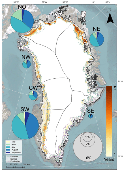
Between 2016 and 2024, slush was detected across all six drainage basins of the GrIS (Fig. 3). Seasonal slush extent, defined here as the area in which slush was detected at least once during a given May–September season, had a mean value of ∼ 48 100 km² ± 3600 km² over the nine-year study period, equivalent to ∼ 2.8 % of the ice sheet. The greatest concentrations of slush typically occurred 10–20 km inland (Fig. 3), although slush was observed as far as 170 km inland in 2019, the highest-melt year of the study period (Fig. 4c).

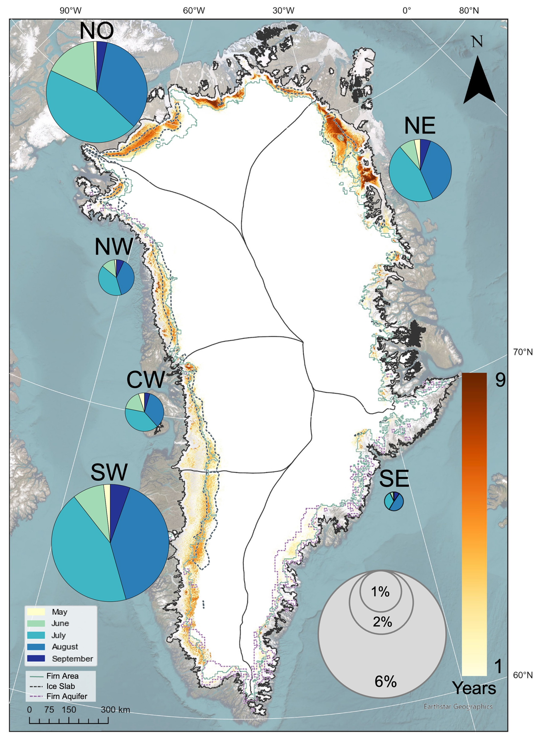
Figure 3 Slush persistence (years) and mean seasonal slush extent (% basin area) across GrIS basins during the May–September melt seasons from 2016–2024. Slush persistence is represented by the colour bar on a scale from 1 year (light yellow) to 9 years (dark orange). The mean seasonal slush extent for each basin from 2016–2024, expressed as a percentage of total basin area, is illustrated by the area of the circles. Within each circle, pie charts display the mean monthly distribution of slush extent averaged over all melt seasons. The green outline depicts mean firn extent (2000–2017) from Vandecrux et al. (2019). Dark grey dashed outlines depict ice slab extents from 2010–2018 (Jullien et al., 2023), and purple dashed outlines depict firn aquifer extents from 2010–2014 (Miège et al., 2016). Base map source: Esri (2024) | Powered by Esri.

Although slush was observed in every basin, its spatial coverage varied across the ice sheet (Fig. 3). Between 2016 and 2024, the SW basin exhibited the greatest proportional coverage (∼ 5.3 % of basin area; 11 190 km² ± 1090 km²), followed by the NO basin (∼ 4.7 %; 11 410 km² ± 630 km²) and the NE basin (∼ 2.9 %; 14 260 km² ± 740 km²). The CW and NW basins both had similar proportional coverage, each corresponding to ∼ 1.9 % of their respective basin area, with mean seasonal extents of 4420 km² ± 440 km² and 5270 km² ± 560 km², respectively. The SE basin showed the lowest proportional coverage (∼ 0.6 %; 1630 km² ± 200 km²).

Slush persistence, defined as the number of melt seasons in which slush was detected at a given location, was examined on an inter-annual basis. Mean persistence was highest in the NE and NO basins, where locations classified as slush were mapped in an average of four out of nine melt seasons. Mean persistence was moderate in the NW and SW basins, at three melt seasons, and lowest in the CW and SE basins, at two melt seasons (Fig. 3).

The cumulative area mapped as slush in at least one melt season between 2016 and 2024 was 143 000 km² ± 5800 km² (∼ 8.2 % of the ice sheet), whereas only 1700 km² ± 220 km² (∼ 0.1 % of the ice sheet) was mapped as slush in all nine melt seasons. The basins that had the largest areas of this highly persistent slush (i.e., slush present in every melt season) were the NE and NO, with 910 km² ± 90 km² and 480 km² ± 80 km², respectively. In the SW basin, despite having one of the highest mean seasonal slush extents over the nine-year period (11 190 km² ± 1090 km²), only 50 km² ± 15 km² of this area was mapped as slush in every melt season.

Slush occurrence was concentrated predominantly over bare ice regions, defined here as areas outside the late-summer firn extent where glacier ice is seasonally exposed at the surface, with ∼ 71 % of all mapped slush occurring in these regions (101 790 km² ± 3660 km²) compared to ∼ 29 % (41 280 km² ± 2220 km²) over firn-covered areas (as delineated by Vandecrux et al., 2019). This partitioning strengthened with increasing persistence, with the proportion of mapped slush occurring in the bare ice area increasing from ∼ 61 % for 1–2 year persistent slush (45 010 km² ± 6000 km²), to ∼ 77 % for 3–5 year slush (38 110 km² ± 4270 km²), and ∼ 91 % for the most persistent (6–9 year) slush (18 670 km² ± 1580 km²), indicating that long-lived slush is increasingly associated with the bare-ice zone. Within the firn zone, overlap with firn aquifers (Miège et al., 2016) remained limited, accounting for only ∼ 5 % of total mapped slush (7610 km² ± 760 km²).

Overlap between our mapped slush and the ice-slab extents mapped by Jullien et al. (2023) ranged from a low-end estimate of ∼ 29 % (40 880 km² ± 760 km²) to a high-end estimate of ∼ 32 % (45 290 km² ± 910 km²) of all mapped slush. This slush–slab coincidence increased with slush persistence: for 1–2-year persistent slush it was ∼ 21 %–24 % (15 360 ± 1410 to 17 850 ± 1650 km²), rising to ∼ 37 %–38 % (7550 ± 610 to 7810 ± 640 km²) for 6–9-year persistent slush. A further ∼ 15 % (21 280 km² ± 1240 km²) under the low-end slab estimate and ∼ 14 % (20 370 km² ± 1160 km²) under the high-end slab estimate of all mapped slush occurred within the firn zone but outside both mapped aquifer and slab extents.

3.2 Ice-sheet-wide inter- and intra-annual variability in slush extent and elevation

The seasonal slush extent across the GrIS varied considerably from year to year, closely reflecting inter-annual variability in snowmelt derived from RACMO (Noël et al., 2019) (Fig. 4). The maximum seasonal areal extent (i.e., the composite slush area from May–September) was lowest in 2018, the least intense melt year of the study period (Fig. 4c), when seasonal slush extent was 18 680 km² ± 2400 km² (∼ 1.1 % of the ice sheet) and RACMO snowmelt anomalies were +2.5 mm w.e. above the 1960–1989 mean, the lowest value during 2016–2024. The largest extent occurred in 2019, the strongest melt year (Fig. 4b), when seasonal slush extent reached 88 490 km² ± 4910 km² (∼ 5.1 % of the ice sheet) and snowmelt anomalies reached +10 mm w.e. above the 1960–1989 mean (Fig. 4b). No statistically significant temporal trend in the maximum seasonal slush extent over the whole ice sheet was observed over the study period.

Figure 4 Mean annual climate and slush variability across the GrIS from 2016–2024. (a) Ice-sheet-wide mean snowfall anomalies (black) and FAC anomalies (teal) relative to the 1960–1989 mean. (b) Ice-sheet-wide mean snowmelt anomalies (black) and 2 m air temperature anomalies (orange) relative to the 1960–1989 mean. (c) Seasonal slush extent for May–September, shown as absolute area (left y-axis, grey bars) and as a percentage of total ice-sheet area (right y-axis; dashed dark-red line). (d) Stacked monthly slush extent for May–September in each year (note: monthly segments are not spatially additive). Snowfall, snowmelt, and 2 m air temperature are derived from RACMO, while FAC is derived from the IMAU-FDM (available through 2023 only).

Superimposed on these inter-annual variations in seasonal slush extent from 2016–2024 was a consistent intra-annual pattern in monthly slush extent, defined here as the composite slush area within a single calendar month, with lowest average values in May and September (typically ∼ 0.2 % of the ice-sheet area over the nine years) and peaks in July (1.8 %) and August (1.5 %) (Fig. 3). This broad intra-annual cycle of low early- and late-season monthly slush extent and mid-melt-season maxima was a defining feature throughout the study period. The cycle was most pronounced in the highest melt year, 2019, when monthly slush extent reached its greatest values in July (53 330 km² ± 3780 km²) and August (66 170 km² ± 3630 km²) (Fig. 4d). However, a notable departure from this cycle occurred in September 2022, when monthly slush extent (15 720 km² ± 1700 km²) surpassed that of August (10 290 km² ± 1480 km²) by ∼ 5430 km² (Fig. 4d).

Inter-annual variability was also evident in the ice-sheet-wide mean upper slush-limit elevation (the average elevation of the highest points at which slush was mapped), ranging from approximately 1420 m a.s.l. in 2018 to 1630 m a.s.l. in 2019 (Fig. 5a). We did not find a statistically significant temporal trend in mean upper-limit elevation at the ice-sheet scale from 2016–2024.

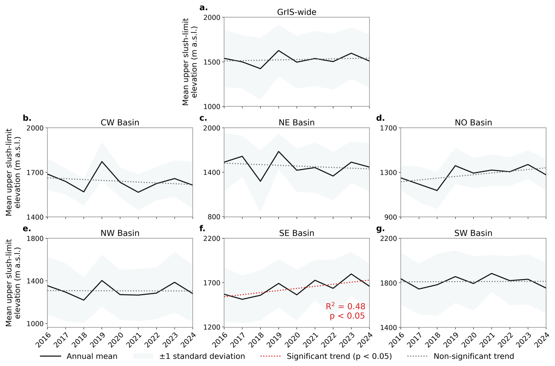
Figure 5 Inter-annual variability in mean upper slush-limit elevation across the GrIS from 2016 to 2024. Panel (a) shows ice-sheet-wide values, while panels (b)–(g) show values for the CW, NE, NO, NW, SE, and SW basins, respectively. Black lines show annual mean upper slush-limit elevation, and shading represents ±1 standard deviation of elevation measurements sampled along the mapped upper slush limit. Dotted lines show fitted linear temporal trends; statistically significant trends (p< 0.05) are shown in red and non-significant trends in grey. Note that y-axis ranges differ among panels.

3.3 Regional inter- and intra-annual variability in slush extent and elevation

At the regional scale, inter-annual variability in slush extent broadly echoed the ice-sheet-wide pattern over the nine-year period (Sect. 3.2), though the magnitude and precise timing of changes differed by region (Fig. 6). In the highest melt year of 2019, all drainage basins experienced peak or near-peak seasonal slush extent, with the greatest proportional coverage in the SW (22 060 km² ± 1340 km²; ∼ 10.5 % of basin area), followed by the NO (16 430 km² ± 580 km²; ∼ 6.8 %), the NE (26 680 km² ± 1240 km²; ∼ 5.5 %), the CW (11 400 km² ± 720 km²; ∼ 4.9 %), and the NW (10 340 km² ± 820 km²; ∼ 3.7 %). Other high-melt years also saw elevated seasonal slush extent in specific regions. For instance, in 2023, the second-highest melt year in the time series, both the NO and SE basins recorded their maximum seasonal slush extents in the time series, reaching 17 370 km² ± 870 km² (∼ 7.1 % of basin area) in the NO and 4510 km² ± 540 km² (∼ 1.6 %) in the SE. Post-2019, the NO basin notably maintained a consistently higher seasonal slush extent than pre-2019 levels, a pattern not observed in any other region.

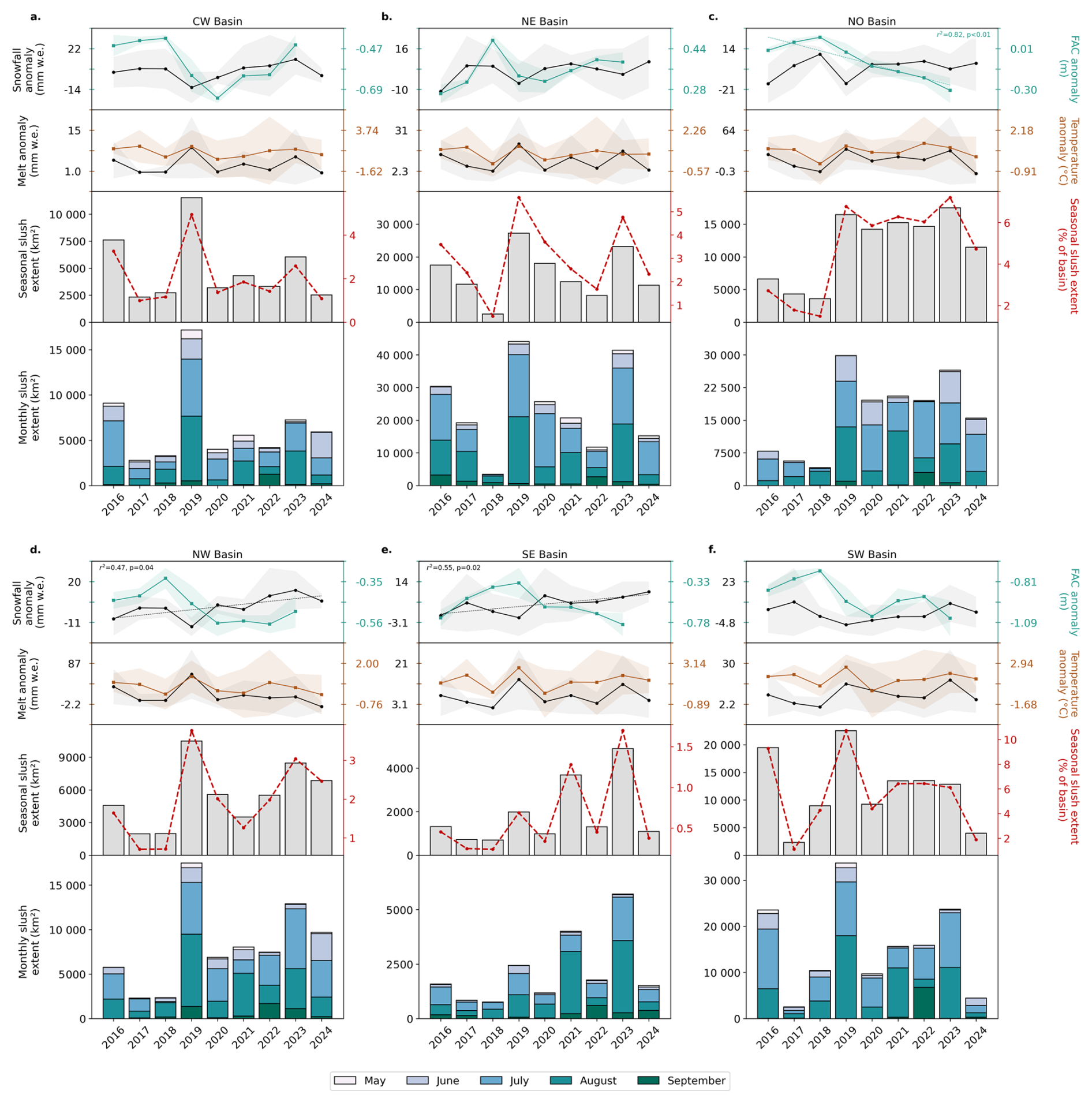
Figure 6 Basin-scale climate and slush variability across the GrIS from 2016–2024, shown for the CW (a), NE (b), NO (c), NW (d), SE (e), and SW (f) basins. Within each subplot, the uppermost panel shows snowfall anomalies (black) and FAC anomalies (teal) relative to the 1960–1989 mean, with statistically significant trends (p<0.05) indicated where present. The second panel shows snowmelt anomalies (black) and 2 m air temperature anomalies (orange) relative to the 1960–1989 mean. The third panel shows maximum seasonal slush extent (May–September) as absolute area (left y-axis, grey bars) and as a percentage of total basin area (right y-axis; dashed red line). The bottom panel shows stacked maximum monthly slush extent for May–September in each year (note: monthly segments are not spatially additive). Snowfall, snowmelt, and 2 m air temperature are derived from RACMO, while FAC is derived from the IMAU-FDM (available through 2023 only).

The intra-annual cycle of monthly slush extent was broadly consistent across basins, but the timing and magnitude of its mid-season peak differed by region (Fig. 6). August 2019 marked the greatest monthly slush extent during the time series for all basins except the SE (Fig. 6). Proportional coverage was greatest in the SW, where slush covered 17 740 km² ± 950 km² (∼ 8.4 % of basin area), followed by the NO (12 500 km² ± 550 km²; ∼ 5.1 %), the NE (19 940 km² ± 970 km²; ∼ 4.1 %), the CW (7300 km² ± 450 km²; ∼ 3.1 %), and the NW (7920 km² ± 610 km²; ∼ 2.8 %). September 2022 saw an atypical late-season resurgence in monthly slush extent that was above the time series average across most basins (Fig. 6). Notably, September 2022 was the month of peak monthly slush extent for the SW basin (Fig. 6f), representing the only instance in the record where the annual maximum monthly slush extent occurred in September rather than July or August. The preceding month, August 2022, recorded substantially lower values across all basins (e.g., SW: 1660 km² ± 280 km², ∼ 0.8 %; NE: 2500 km² ± 360 km², ∼ 0.5 %), highlighting the atypical nature of this late-season peak.

The mean upper slush-limit elevation varied markedly between basins and years (Fig. 5). Slush generally extended to higher elevations during high-melt years, including 2019 (e.g., CW: 1770 m a.s.l.; NE: 1680 m a.s.l.; NO: 1360 m a.s.l.) and 2023 (e.g., SE: 1800 m a.s.l.; NW: 1390 m a.s.l.), while mean upper slush-limit elevations were lower during reduced-melt years such as 2018 and 2020 (e.g., NE: 1280 m a.s.l. in 2018; NW: 1270 m a.s.l. in 2020). Some basins showed distinct inter-annual changes in mean upper slush-limit elevation; for example, the NE basin experienced an increase of approximately 400 m between 2018 and 2019. Notably, the highest mean upper slush-limit elevation did not always coincide with the year of peak slush extent; for instance, the SW reached its highest mean upper slush-limit elevation in 2021 (1880 m a.s.l.), two years after its areal maximum in 2019 (Fig. 5g). A weak but statistically significant increasing temporal trend in mean upper slush-limit elevation was observed in the SE basin from 2016 to 2024, with a mean increase of 23.5 m yr⁻¹ (R²=0.48; p<0.05; Fig. 5f). No other basins exhibited statistically significant temporal trends in mean upper slush-limit elevation during the study period.

We found a significant positive relationship between annual mean upper-limit elevation and maximum seasonal slush extent across all basins (p<0.05; Fig. 7). The strength of this relationship varied regionally, with the strongest relationships in the NO (R²=0.91) and SE (R²=0.81) basins, moderate relationships in the CW (R² = 0.74), SW (R²=0.70), and NE (R²=0.60) basins, and a weaker relationship in the NW basin (R²=0.49).

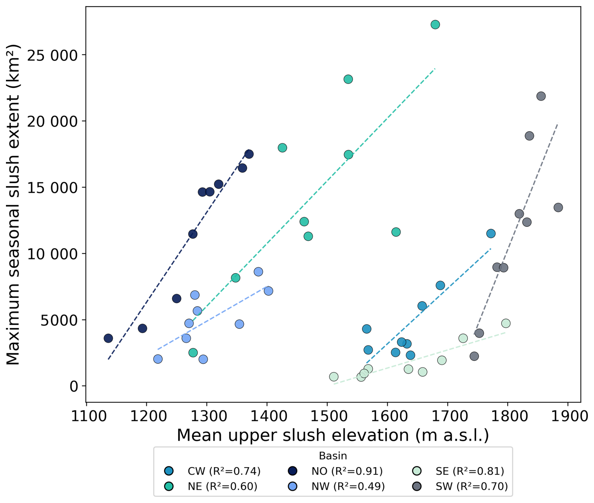
Figure 7 Relationship between mean upper slush-limit elevation and maximum seasonal slush extent by basin (2016–2024). Coloured points show seasonal values, and dashed lines show ordinary least-squares regressions fitted separately for each basin. Reported R² and p-values refer to these regressions; all relationships are statistically significant (p<0.05).

3.4 Potential environmental controls on slush extent and occurrence

At the inter-annual basin-wise scale, mean seasonal slush extent throughout May–September was positively correlated with snowmelt averaged across the potential slush zone (Fig. S6): NE (ρ= 0.99, p<0.001), SW (ρ= 0.90, p<0.001), NO (ρ= 0.75, p<0.05), SE (ρ= 0.75, p<0.05), and CW (ρ= 0.70, p<0.05). April–June snowmelt also correlated positively in NE (ρ= 0.95, p<0.001) and NO (ρ= 0.68, p< 0.05). Seasonal slush extent correlated positively with 2 m air temperature during May–September in NE (ρ= 0.80, p< 0.01), and during April–June in NE (ρ= 0.77, p< 0.05) and SW (ρ= 0.67, p< 0.05). Negative relationships with snowfall occurred during January–March in CW (ρ= −0.77, p< 0.05) and April–June in NE (ρ= −0.73, p< 0.05). May–September FAC was negatively correlated with seasonal slush extent in all basins, although none of these relationships were statistically significant. These inter-annual correlations were based on nine annual observations per basin, or eight for FAC, and should therefore be treated cautiously.

At the intra-annual basin-wise scale, monthly slush extent during May–September was positively correlated with snowmelt across all basins (Fig. S7), most strongly in CW and SW (both ρ= 0.89, p < 0.001) and NO (ρ= 0.86, p<0.001). Previous-month snowmelt also correlated positively with monthly slush extent across all basins (ρ= 0.41–0.80, all p < 0.01). Monthly slush extent was positively correlated with 2 m air temperature across all basins (Fig. S8; ρ= 0.69–0.88, all p<0.001), with generally weaker associations for previous-month temperature. Monthly slush extent correlated negatively with FAC (Fig. S9) in NE (ρ= −0.65), SE (ρ= −0.55), NW (ρ= −0.54), NO (ρ= −0.53), and CW (ρ= −0.32) (all p < 0.05), with no significant relationship in SW; previous-month FAC was significant only in NE (ρ= −0.31, p < 0.05). Relationships between monthly slush extent and snowfall were generally weak and non-significant (Fig. S10), except negative relationships with concurrent snowfall in SE (ρ= −0.59, p< 0.001) and NE (ρ= −0.30, p< 0.05), and previous-month snowfall in SE (ρ= −0.45, p< 0.01).

Across the potential slush zone, slush occurrence (i.e., whether slush was mapped within a grid cell during a given May–September season) was most frequent under combinations of lower March FAC and greater spring snowmelt (Fig. S11). Slush-present grid-cell–years had lower median March FAC than slush-absent grid-cell-years (0.16 versus 8.90 m) and greater median April–June snowmelt (158 versus 68 mm w.e.). This pattern also occurred in all individual basins. A one-standard-deviation increase in March FAC was associated with a 59 % reduction in the odds of slush occurrence (odds ratio = 0.41, p < 0.001), whereas a one-standard-deviation increase in spring snowmelt was associated with a 71 % increase in the odds of slush occurrence (odds ratio = 1.71, p < 0.001). However, the substantial overlap between slush-present and slush-absent conditions indicates that neither March FAC nor spring snowmelt alone defined a distinct threshold for slush occurrence.

3.5 First-order assessments of the wider impact of slush

Applying the empirical meltwater-albedo framework of Ryan et al. (2025) to our ice-sheet-wide slush observations provides a first estimate of potential radiative and melt-equivalent implications of slush at the scale of the whole ice sheet. We found that estimated daily excess energy absorption ranged from approximately 53 PJ d⁻¹ in 2018, when seasonal slush extent was ∼ 18 700 km², to 249 PJ d⁻¹ in 2019, when seasonal slush extent reached ∼ 88 500 km². The mean value across 2016–2024 was 134 PJ d⁻¹. Converted to an equivalent mass of ice melt and weighted by the observed distribution of monthly slush extent, cumulative additional melt ranged from 4.9 Gt yr⁻¹ (2018) to 23.0 Gt yr⁻¹ (2019), with a 2016–2024 mean of 12.4 Gt yr⁻¹. Restricted to RACMO's modelled runoff zone, mapped slush covered 13 % of runoff-zone pixels on average (range: 6 % in 2018 to 22 % in 2019). The runoff currently modelled from these slush-covered pixels totalled 30.7 Gt yr⁻¹ on average (range: 11.8–63.6 Gt yr⁻¹); this would increase to approximately 42.0 Gt yr⁻¹ if the additional energy absorbed due to slush-driven surface darkening were fully converted to ice melt rather than retained within the firn.

4 Discussion

To the best of our knowledge, our work forms the first large-scale assessment of slush on the GrIS. Prior assessments have almost exclusively focused on well-defined supraglacial meltwater features, specifically lakes, channels, and water-filled crevasses (e.g., Dunmire et al., 2021, 2025; Zhang et al., 2023; Melling et al., 2024; Fan et al., 2025) that are somewhat easier to map using traditional thresholding methods. By leveraging ML within a cloud-based framework, we show that slush can be systematically mapped across the entire GrIS. The resulting nine-year, ice-sheet-wide dataset offers new insight into the spatial variability and persistence of slush, revealing that slush is a widespread and climatically sensitive component of the surface hydrological system on the GrIS.

4.1 Slush dominates the areal extent of surface meltwater on the GrIS

Between 2016 and 2024, slush was detected across a mean seasonal extent of 2.8 % (∼ 48 100 km²) of the GrIS, with the largest extent of 5.1 % (∼ 88 500 km²) occurring in 2019, the highest-melt year of our study period (Figs. 3 and 4). In the same year, Zhang et al. (2023) mapped a maximum area of 9990 km² for lakes, channels, and water-filled crevasses; the mapped seasonal slush extent was therefore approximately nine times larger than the combined area of these other meltwater features. Even in the lowest melt year of our study period, 2018, our mapped seasonal slush extent (1.1 %; ∼ 18 700 km²) was nearly four times greater than the 4900 km² of other meltwater features reported by Zhang et al. (2023) for 2018. Studies focusing solely on supraglacial lakes highlight an even greater disparity. Fan et al. (2025) showed that between 1985 and 2023, supraglacial lake area rarely exceeded 3500 km², with a total of ∼ 3000 km² in 2019. Additionally, compared with the ice-sheet-wide supraglacial lake extents reported by Dunmire et al. (2021) of 1240 km² in 2018 and 2570 km² in 2019, the total seasonal slush extent mapped in our study was approximately 15-fold greater in 2018 and 34-fold greater in 2019. At the basin scale, our seasonal slush extent observations also greatly surpass the areal extent of other meltwater features observed previously. For example, for the NE in 2019, we detected a maximum seasonal slush extent of ∼ 26 680 km², whereas Zhang et al. (2023) reported just 820 km² of other meltwater features in this basin – a more than 30-fold difference. Although the aforementioned cross-study comparisons for the GrIS reflect differing methodologies, they are used here to provide first-order context for the relative spatial coverage of slush compared to other surface meltwater features. Given that slush has been largely overlooked in previous studies, this comparison highlights its widespread presence across the GrIS.

The dominance of slush on the GrIS relative to lakes also contrasts strongly with Antarctic ice shelves, where slush and lakes occupy approximately equal areas, with slush contributing ∼ 50 % of peak-summer (January) meltwater area across 57 ice shelves (Dell et al., 2024). The higher slush proportion on the GrIS likely reflects fundamental differences in glaciological setting and climate relative to Antarctic ice shelves, with the former experiencing substantially stronger melt intensity (van den Broeke et al., 2023; Hanna et al., 2024), reduced FAC (The Firn Symposium Team, 2024), widespread bare-ice exposure (Ryan et al., 2019), and recurrent near-surface saturation due to ice slabs and lenses (Culberg et al., 2021; Machguth et al., 2016). Together, these factors allow slush to expand across broad contiguous zones on the GrIS. In contrast, in Antarctica, lake and slush formation is predominantly restricted to flatter ice shelves (Stokes et al., 2019), where lower melt magnitudes, colder mean conditions, and almost complete refreezing of meltwater within the firn (van den Broeke et al., 2023; Banwell et al., 2023) limit the spatial coverage and persistence of all forms of surface meltwater, compared to the GrIS. As Antarctic surface hydrology may increasingly come to resemble present-day Greenland under future warming (Bell et al., 2018; Mottram et al., 2025), improving process-level understanding of slush dynamics across both ice sheets is an urgent research priority.

4.2 Slush is most extensive in the western and northern basins

Our observations reveal that slush is most extensive in the western (notably the SW) and northern basins of the GrIS, and least extensive in the southeastern basin. This distribution aligns with observations from previous studies of supraglacial meltwater features, particularly supraglacial lakes, which report greater prevalence in west Greenland (e.g., Selmes et al., 2011; Dunmire et al., 2021, 2025; Hu et al., 2022; Zhang et al., 2023; Fan et al., 2025).

In the SW basin, low-angle slopes, broad ablation zones (Ryan et al., 2019), and high melt rates (Mikkelsen et al., 2016; van As et al., 2017) create conditions that likely allow slush to extend further inland than in other regions. A disproportionate loss of FAC relative to other regions (Vandecrux et al., 2019) may also promote widespread surface saturation and slush formation in the SW by reducing the capacity of the firn column to accommodate meltwater. Although these conditions favour extensive inland slush in much of the SW basin, the western margin coincides with the “dark zone”, where low-albedo impurities sustain prolonged bare-ice exposure (Tedstone et al., 2017; Feng et al., 2024), leaving little snow or firn substrate for slush to form, consistent with the stripe of low slush persistence we identify along the western ice-sheet margin (Fig. 3).

The dominance of slush in the western and northern regions may also reflect the distribution of surface and subsurface structures that restrict vertical meltwater infiltration. A substantial proportion of mapped slush (∼ 71 %) occurs within the bare-ice region, which is seasonally snow-covered but exposed as ice by late summer, where the surface forms an inherently impermeable boundary to downward percolation. The spatial coincidence between mapped slush and ice-slab extents suggests that subsurface ice slabs may influence slush distribution by acting as shallow permeability barriers within the firn column. By restricting vertical percolation, slabs promote sustained saturation of the overlying firn and favour lateral meltwater routing, creating conditions conducive to recurrent slush formation (Machguth et al., 2016; MacFerrin et al., 2019; Jullien et al., 2023). Approximately 30 % of Greenland's mapped slush area overlaps with slab extents, with most of this concentrated in the western and northern basins (Fig. 3). In these regions, more persistent slush is often coincident with slab presence, potentially reflecting a positive feedback: meltwater routed laterally through the slush zone ponds in low-gradient areas above the slab, where repeated refreezing thickens the slab and reinforces the permeability barriers that favour recurrent slush formation, consistent with field observations by Tedstone et al. (2025).

Unlike slabs, firn aquifers are characterised by the deep infiltration of meltwater into temperate firn and long-term subsurface water storage rather than shallow blockage of vertical flow (Forster et al., 2014; Miège et al., 2016), and can host ice layers (e.g., Miller et al., 2020). Comparatively limited overlap of aquifers with mapped slush suggests that they exert less sustained control on slush persistence than shallow impermeable ice layers.

Notably, a non-trivial fraction of all mapped slush (∼ 15 %) occurs within firn areas outside both mapped ice slab and firn aquifer extents, with much of this slush concentrated in western Greenland. While recurrent slush formation in bare ice regions is expected due to the impermeable ice surface, these observations indicate that persistent slush can also develop in firn regions lacking extensive perennial low-permeability units. In these settings, smaller-scale ice lenses and contrasts in firn density and grain size may locally restrict vertical percolation, promoting lateral spreading and near-surface saturation, consistent with experimental observations from Greenland firn (Humphrey et al., 2021). Periods of intense melt may further enhance these effects where meltwater production exceeds local infiltration capacity. Together, these patterns suggest that finer-scale firn stratigraphic heterogeneity may exert an important control on recurrent slush formation across parts of the ice sheet.

4.3 Slush reaches higher elevations and is greater in areal extent during extreme melt years

In extreme melt years (notably 2019 and 2023; the highest and second highest melt years in our time series, respectively), slush both reaches higher elevations and is more areally extensive than in cooler, low-melt years (e.g., 2018; Figs. 5 and 6), which also mirrors the established tendency for supraglacial lakes to appear at higher elevations in warmer years (Sundal et al., 2009; Liang et al., 2012; Lüthje et al., 2006; Leeson et al., 2015; Glen et al., 2025). Under typical conditions, we show that variability in the monthly slush extent follows a predictable seasonal cycle, forming in May, peaking in area in July, and decreasing in area during the autumn freeze-up, similar again to the behaviour of supraglacial lakes (e.g., Otto et al., 2022; Glen et al., 2025). During extreme melt years such as 2019, this seasonal cycle is amplified, with sustained high air temperatures combined with melt-albedo feedbacks producing prolonged, intense melt (Sasgen et al., 2020; Tedesco and Fettweis, 2020; Hanna et al., 2021), which likely drove 2019 to have the most extensive and furthest inland slush in our record. In contrast, we suggest that the atypical pattern in 2022 resulted from a late-season, anomalously warm and rainy event in September 2022 that triggered ice-sheet-wide melt and delayed late-season freeze-up (Moon et al., 2022; Copernicus Climate Change Service (C3S), 2023), enabling the sustained slush presence that we observed into late September 2022.

Despite the strong inter-annual variability in slush area and mean upper-limit elevation that we observed, our nine-year record reveals no statistically significant temporal trend in either variable at ice-sheet or basin scales, except for a weak increase in mean upper-limit elevation in the SE basin (R²= 0.48, p < 0.05). These results are consistent with those of Machguth et al. (2022), who found no significant change in maximum slush elevation on the western GrIS over a study period of similar length (2013–2021) but observed pronounced intra-seasonal variability. Multi-decadal studies, however, have reported increases in meltwater feature area and elevation over time. For example, Fan et al. (2025) documented an ice-sheet-wide supraglacial lake area increase of ∼ 50.5 km² yr⁻¹ from 1985–2023, while Tedstone and Machguth (2022) reported increases in visible runoff limits of ∼ 242 m (west), 194 m (north), and 59 m (northeast) between 1985–2020. These findings suggest that while inter- and intra-annual variability dominate decadal slush records, slush is nonetheless likely to follow the broader trajectory of increasing area and elevation over multi-decadal timescales.

Our observations suggest that extreme melt events may not only drive widespread slush formation through direct surface melting, but also alter firn structure in ways that promote slush recurrence in later seasons. For example, the northern basin exhibited elevated seasonal slush extent in every year following the extreme 2019 melt season (Fig. 6c), including years characterised by relatively low melt. This pattern points to a possible legacy effect, whereby slush formed during 2019 subsequently refroze to produce low-permeability firn and/or thicken pre-existing ice slabs, reducing firn infiltration and storage capacity. The strong and statistically significant decline in FAC between 2016 and 2023 (R²= 0.82, p < 0.01; Fig. 6) is consistent with this, and under such reduced-storage conditions, saturation of the seasonal snowpack alone may be sufficient to regenerate slush from one year to the next. Rawlins et al. (2023) similarly documented earlier melt onset and prolonged melt seasons in northern Greenland following major slush events in preceding years. As the GrIS warms, declining firn storage capacity, expanding ice slabs, and more frequent extreme melt events may therefore not only increase slush extent but also progressively alter the conditions under which slush forms, persists, and refreezes, raising the possibility that legacy effects influence future meltwater production beyond melt forcing alone. However, the processes underlying this pattern cannot be resolved from our observations alone, and the proposed mechanism requires further investigation.

4.4 Slush extent and occurrence are associated with meltwater supply and firn storage capacity

We find that slush extent is positively associated with snowmelt at the intra-annual scale across all basins, and inter-annually in most basins, consistent with increased meltwater supply exceeding available pore space and sustaining near-surface saturation and lateral water redistribution. At the intra-annual scale, both antecedent and concurrent snowmelt correlate with monthly slush extent, suggesting that wetted firn can remain saturated into subsequent months. This finding is consistent with field evidence that saturation in firn and slush can persist for days after a reduction in melt intensity (Clerx et al., 2022). A positive association between 2 m air temperature and slush extent is also evident, particularly at the intra-annual scale. Because temperature strongly influences snowmelt, this relationship likely reflects greater meltwater production rather than an independent control on slush formation.

We also find a negative association between slush extent and FAC. One possible explanation is that lower FAC limits the amount of meltwater that can be retained or refrozen before near-surface saturation is reached (Harper et al., 2012), consistent with FAC's established role in Greenland meltwater retention (e.g., Vandecrux et al., 2019). However, because ∼ 71 % of mapped slush occurred within the late-summer bare-ice zone, where FAC is inherently low, the negative association may partly reflect differences between bare-ice and firn-covered regions. The relationship between slush extent and FAC is clearest at the intra-annual scale, where monthly slush extent is negatively correlated with FAC in five of the six basins. Inter-annual correlations between seasonal slush extent and FAC are also negative across all basins but are not statistically significant, potentially because the FAC record contains only eight annual observations per basin (2016–2023). Previous-month FAC is significantly associated with monthly slush extent in only one basin, whereas previous-month snowmelt is significant across all basins, suggesting that meltwater supply has a more immediate association with monthly slush extent, while FAC is slower-changing, with firn structural changes capable of persisting for decades (The Firn Symposium Team, 2024). FAC represents potential firn storage rather than the pore space necessarily accessible to meltwater, and modelled FAC may overestimate available storage in ice-slab-affected regions, where near-surface ice layers restrict percolation into deeper firn (Machguth et al., 2016; MacFerrin et al., 2019) – a limitation not captured by IMAU-FDM (Brils et al., 2022).

Snowfall exhibits weaker and more spatially inconsistent relationships with slush extent than the other variables. Where statistically significant, these relationships are negative and limited to a small subset of basins and time windows. This pattern suggests that greater snowfall is associated with reduced slush extent, potentially because a deeper snowpack increases near-surface meltwater-storage capacity or maintains a higher surface albedo, thereby limiting melt and delaying saturation (The Firn Symposium Team, 2024).

Across the ice sheet and within individual basins, slush occurrence (i.e., whether a grid cell was mapped as slush during May–September in a given year) is more likely under greater spring snowmelt and lower March FAC. Neither variable shows a distinct threshold for slush occurrence: slush occurs across a broad range of FAC and snowmelt conditions, with low FAC favouring slush occurrence but not determining it independently of meltwater supply. This contrasts with the threshold-like pattern reported for Antarctic ice shelves, where meltwater coverage remained below 1 % above approximately 21 m FAC but exceeded 5 % below approximately 14 m FAC, although these values were derived from ice-shelf-averaged FAC and meltwater coverage (Dell et al., 2024). Our grid-cell-level results instead indicate that slush occurrence on the GrIS reflects the combined influence of FAC and snowmelt, alongside local conditions not represented by either variable alone. Dell et al. (2024) similarly suggest that spatially averaged FAC may obscure controls operating at finer spatial scales.

4.5 Slush has implications for GrIS mass loss

Slush may influence surface energy balance and meltwater pathways, yet it remains poorly represented in models of ice-sheet surface energy balance (e.g., Noël et al., 2019; Huai et al., 2020), lake formation (e.g., Law et al., 2020), and hydrological routing (e.g., Banwell et al., 2012; Leeson et al., 2012; Gantayat et al., 2023). Accurately representing its distribution and dynamics is important for capturing albedo–melt feedbacks, meltwater storage, and connectivity between supraglacial hydrological features. The ice-sheet-wide observations presented here provide new constraints for developing these models, although our first-order analyses should not be interpreted as fully constrained physical estimates.

To place our slush melt estimate in the broader context of GrIS mass loss (Sect. 3.5), we find that the mean potential additional melt associated with slush-driven energy absorption (12.4 Gt yr⁻¹ over 2016–2024) is equivalent to approximately 7 % of the ice sheet's mean annual mass loss (169 ± 9 Gt yr⁻¹ over 1992–2020; Otosaka et al., 2023) and 15 % of an estimated runoff-driven component of 85 Gt yr⁻¹, calculated by applying the runoff contribution of 50.3 % reported for 1992–2018 (The IMBIE Team, 2020) to this mean annual mass-loss value. These estimates are subject to substantial uncertainty because the empirical coefficient used in the calculation was derived from open meltwater ponds and has not been validated for slush, and because the optical properties and albedo-lowering effect of slush remain poorly constrained (Ryan et al., 2025). Nevertheless, the greater areal extent of slush relative to open meltwater suggests that its contribution to surface darkening and melt amplification could be substantial. If the additional absorbed energy were converted to melt, runoff from slush-covered areas could exceed current estimates from regional climate models – though such comparisons are further complicated by model uncertainty in the spatial extent of the runoff zone (Machguth et al., 2026). Explicitly incorporating slush into physically based surface mass-balance and hydrological models will therefore be important for constraining its influence on GrIS evolution under continued warming.

5 Conclusion

We present the first ice-sheet-wide record of slush across the GrIS, spanning nine melt seasons from 2016 to 2024. Using a cloud-based machine-learning framework, we show that slush is widespread, responsive to melt conditions, and the dominant mapped surface meltwater feature by seasonal extent. During high-melt years, seasonal slush extent was up to an order of magnitude greater than reported estimates of the combined extent of supraglacial lakes, channels, and water-filled crevasses. Slush is most extensive in the southwestern and northern basins, most persistent in the northeast and north, and extends to higher elevations during intense melt years. These spatial and temporal patterns likely reflect variations in bare-ice exposure, ice-slab distribution, and firn properties across the ice sheet. We also find that both slush extent and occurrence are associated with higher snowmelt and lower FAC.

Despite its widespread occurrence and marked seasonal variability, slush remains largely absent from surface mass-balance, hydrological, and coupled ice-dynamics models used to project future ice-sheet behaviour. This omission may become increasingly important as the GrIS evolves under continued warming. First-order estimates suggest that slush-driven surface darkening may increase surface energy absorption and, if this additional energy is converted to melt, enhance runoff. Explicitly representing slush alongside other surface meltwater features is therefore important for developing a more complete understanding of the GrIS response to climate change. The nine-year dataset presented here provides an observational foundation for improving representations of the evolving GrIS hydrological system.