A State-Space Model for Monitoring Greenland Ice Sheet Surface Elevation Change from CryoSat-2

Monitoring surface elevation change of the Greenland Ice Sheet at monthly resolution is important for resolving both seasonal variability and long-term trends, yet irregular sampling and data gaps in satellite altimetry make the reconstruction of consistent spatio-temporal records challenging. We present a data-driven State Space Model (SSM) framework, the Three-Dimensional Elevation Change Model (3D-ECM), for deriving monthly surface elevation changes of the Greenland Ice Sheet from CryoSat-2 radar altimetry data. Unlike approaches with pre-defined seasonal models, seasonality here emerges directly from the data, enabling the detection of seasonal cycles and long-term trends. The method combines a Gaussian Markov Random Field for spatial dependence with an autoregressive process for temporal correlations, allowing robust signal extraction even in regions with sparse or irregular sampling. With this framework, we derive monthly surface elevation changes for the Greenland Ice Sheet in 5 km resolution over the period 2011–2025.

Validation against independent datasets shows strong agreement. At three selected Automatic Weather Station (AWS) sites representing different climatic regimes of the Greenland Ice Sheet, Pearson correlation coefficients between our surface elevation change (dSEC) product and AWS-derived surface elevation records range from 0.58 to 0.7, while comparisons with time series derived from a fusion between laser-altimetry observations and a firn densification model yield correlation coefficients of up to 0.76. Additional comparisons with ICESat-2 and NASA Operation IceBridge airborne data confirm that the applied spatio-temporal post-processing of the dSEC fields reduces the standard deviation by approximately 40 %–45 % while maintaining minimal bias. Furthermore, intercomparison with two published Greenland-wide SEC products derived from satellite altimetry demonstrates that dSEC achieves lower misfit relative to ICESat-2 ATL15, indicating improved agreement with independent laser altimetry.

The resulting monthly surface elevation change data set captures both seasonal variability and long-term trends across the Greenland Ice Sheet. The flexible and fully data-driven 3D-ECM framework is directly transferable to other altimetry missions and multi-sensor records, offering a pathway toward continuous, long-term monitoring of ice-sheet elevation change across satellite generations.

1 Introduction

The Arctic has been warming at up to four times the global average since 1979 (Rantanen et al., 2022; Chylek et al., 2022; Sweeney et al., 2023). This rapid atmospheric warming has accelerated the mass loss from the Greenland Ice Sheet (GrIS) over the last decades (Khan et al., 2022; Løkkegaard et al., 2024), contributing to global sea-level rise (Moon et al., 2018; Mouginot et al., 2019; Box et al., 2022; Khan et al., 2022; Otosaka et al., 2023). Rising sea levels will impact coastal communities worldwide in the coming decades (Bamber et al., 2010; Gardner et al., 2013; Forsberg et al., 2017; Otosaka et al., 2023).

Accurate and timely data on ice sheet dynamics are therefore essential for understanding the processes driving mass loss and refining projections of future sea-level rise (Williams et al., 2021). Satellite radar altimetry has emerged as a powerful technique for monitoring ice sheet Surface Elevation Change (SEC), which, under certain assumptions, can be converted into estimates of ice sheet mass loss and sea-level contribution (Simonsen et al., 2021). ESA’s CryoSat-2, carrying the SAR Interferometric Radar Altimeter (SIRAL) (Wingham et al., 2006), was specifically designed to measure SEC in ice-covered regions, regardless of cloud cover or solar illumination, making it particularly valuable for the polar regions. With more than a decade of continuous observations, CryoSat-2 provides an unprecedented record for assessing both long-term trends and shorter-term variability in GrIS SEC (Lai and Wang, 2022; Ravinder et al., 2024).

Capturing seasonal fluctuations and short-term events, such as glacier calving or enhanced meltwater runoff, requires a higher temporal resolution than the traditional SEC products derived from radar altimetry (Simonsen et al., 2017; Sørensen et al., 2018). Conventional approaches, such as the plane-fit algorithm (Simonsen et al., 2017; Sørensen et al., 2018), constructs annual SEC by extracting a mean SEC over a multi-year period, but this limits their ability to resolve seasonal fluctuations and short-term events. As a result, much of the seasonal signal and many episodic anomalies remain hidden in aggregated annual products. To address this, new processing methods have been developed to derive monthly SEC from radar altimetry (Lai and Wang, 2022; Zhang et al., 2022; Ravinder et al., 2024; Nilsson et al., 2024; Helm et al., 2024; Khan et al., 2025). These efforts mark a major step forward as they provide a finer temporal detail, which enables more direct comparison and joint analysis with regional climate model outputs and in situ observations.

Recent studies have demonstrated advances in deriving monthly SEC products from altimetry (Zhang et al., 2022; Khan et al., 2025). Different methodological choices are made regarding spatio-temporal regularization and uncertainty treatment. Quantitative comparison against independent laser altimetry, together with inter-comparison against published SEC products, therefore provides a valuable way to place new developments in context. In this study, we evaluate the performance of our state-space framework relative to published SEC products and inter-compare against ICESat-2 ATL15, Operation IceBridge, AWS stations and Surface Elevation Reconstruction And Change detection (SERAC) timeseries.

Here, we address the spatio-temporal reconstruction step of radar altimetry processing by introducing a state space modeling framework that reconstructs monthly gridded SEC fields directly from irregular satellite observations. We integrate state-space models (SSMs) with radar altimetry as a statistical framework to reconstruct spatially and temporally coherent SEC fields from irregular observations, while accounting for measurement uncertainty and spatio-temporal dependence. SSMs have already demonstrated their potential in related Earth Observation applications, for example, in deriving temporally densified water level time series for a river based on multi-mission satellite altimetry (Nielsen et al., 2022). This flexible and data-driven SSM framework can be applied across satellite altimetry missions to generate continuous, gap-filled SEC time series, with seasonal signals emerging directly from the data rather than from predefined models such as in previous studies by e.g. Sørensen et al. (2018) or Khan et al. (2025). In addition, SSMs explicitly separate signal from noise, and are able to handle irregular or missing data, and may provide coherent uncertainty estimates while accounting for spatial and temporal dependencies (Kristensen et al., 2016). Extending this methodology to ice sheets provides a powerful means to generate continuous, gap-filled time series of SEC across a range of spatial and temporal scales, independent of the specific satellite mission.

In this study, we develop our model 3D-ECM to derive monthly surface elevation change (dSEC) over the entire Greenland Ice Sheet from CryoSat-2 radar altimetry data, where the prefix “d” denotes that the model can be configured to any desired temporal resolution; here it is applied at monthly intervals. The derived dataset contains monthly SEC estimates that reflect both multi year trends and intra-annual variations derived from the SSM.

2 Data sets

The construction of the dSEC data product is based on CryoSat-2 Level-2 altimetry data and is validated against independent datasets from ICESat-2, Operation IceBridge (OIB), Automatic Weather Stations (AWS), and laser altimetry-based SERAC time series fusion, incorporating firn height change estimation.

2.1 CryoSat-2 data

CryoSat-2 is a radar altimetry satellite mission developed by the European Space Agency (ESA) to monitor changes in the cryosphere. The SIRAL radar onboard CryoSat-2 operates at Ku band (13.5 GHz). Over the ice sheet margins, it leverages its two antennas to provide synthetic aperture radar interferometric (SARIn) mode, while it only collects single-pulse, nadir-looking data in low-resolution mode (LRM) over the ice sheet interior (Bouzinac, 2019).

In this study, we use Point Of Closest Approach (POCA) elevations available from CryoSat-2 Level-2 SARIn and LRM data products from baseline E (Bouzinac, 2019) as the primary input for estimating monthly dSEC over the Greenland Ice Sheet. POCA elevations theoretically represent the point on the ground closest to the radar beam direction, where the strongest radar return is assumed to originate. The Level-2 data include geophysical corrections such as ionospheric delay, wet and dry tropospheric path delays, solid Earth and ocean tides, and surface scattering corrections. In LRM mode, the SIRAL pulse-limited footprint covers approximately 2.15 km², with an effective diameter of about 1.65 km. In SAR/SARIn mode, the across-track pulse-limited footprint is similarly  1.65 km, while the along-track beam-limited footprint is approximately 305 m (yielding an effective along-track resolution of  400 m), resulting in a total Doppler-limited illuminated area of  0.5 km² (Bouzinac, 2019).

2.2 ICESat-2 validation data

To validate the dSEC derived from CryoSat-2, we use data from NASA's ICESat-2 mission, which provides high-resolution laser altimetry observations over the GrIS. Specifically, we use the ATL15 gridded SEC product (Smith et al., 2022) provided at 1 km spatial resolution. For consistency with the CryoSat-2 dSEC product, the ATL15 data were regridded from its native 1 km EPSG:3413 grid to a regular 5 km EPSG:3413 grid using linear interpolation.

We use ATL15 lag-8 data, which correspond to 24-month SEC estimates centered around each observation month. This lag setting provides a balance between temporal resolution and spatial coverage, allowing a meaningful comparison of the long-term trend with our monthly gridded dSEC product derived from CryoSat-2.

2.3 Operation IceBridge Validation Data

To complement the satellite dataset, we also validate against data from NASA’s OIB mission, which provides airborne laser altimetry measurements over the polar regions from 2009 to 2019 (Studinger et al., 2014). OIB was designed to bridge the observational gap between the ICESat and ICESat-2 missions, providing detailed measurements of ice sheet topography with high spatial resolution and accuracy.

Here, we use OIB Level-4 SEC data derived from repeated airborne laser altimetry tracks (Studinger et al., 2014). The irregular OIB observations are spatially aggregated to the 5 km CryoSat-2 grid using a median binning approach, requiring at least 10 observations per grid cell.

We use data from the OIB campaigns between 2011 and 2016 over the Greenland Ice Sheet, focusing on regions that spatially overlap with our CryoSat-2 dSEC coverage.

2.4 Seasonal surface height change from accumulation and ablation at Automatic Weather Stations

The seasonal amplitudes in our dSEC product are evaluated with data from the Programme for Monitoring of the Greenland Ice Sheet (PROMICE) (Ahlstrøm et al., 2008) and the Greenland Climate Network (GC-Net) AWS (Fausto et al., 2021; Vandecrux et al., 2024). AWS sites are divided between accumulation sites, where snow accumulated in winter does not melt away in the summer, and ablation sites, where the winter snow melts away and is followed by melting of the glacial ice.

A near-continuous record of surface height relative to the AWS's installation height is derived by merging data from multiple instruments (Vandecrux et al., 2024) (variable: z_surf_combined). At ablation sites, it combines data from a station-mounted sonic ranger, a stake-mounted sonic ranger, and a borehole pressure transducer. During ablation periods, the pressure transducer (or, if failing, the stake-mounted sonic ranger) defines surface height, while winter values are based on the adjusted average of both sonic ranger heights. The record is manually corrected for shifts that may occur during maintenance.

These AWS surface heights are not absolute heights, as they are referenced to the installation height and hence only represent the accumulation and ablation that occur at the ice sheet surface. At accumulation sites, the AWS does not capture the surface height change stemming from firn compaction below the station's anchoring depth. They do not include bedrock-related motion, which contributes 1–2 cm uplift every year (Liu et al., 2017), nor thinning or thickening of the ice below, which may contribute to surface height changes of the same order of magnitude as changes caused by surface melt (Bevan et al., 2015; Kehrl et al., 2017). Yet, in the absence of Greenland-wide, temporally resolved maps of dynamic elevation change, the AWS-derived surface heights provide an independent estimate of local seasonal surface-height variability. Differences between AWS observations and dSEC may occur in dynamically active regions, where the satellite-derived elevation changes also include dynamic ice-thickness variations.

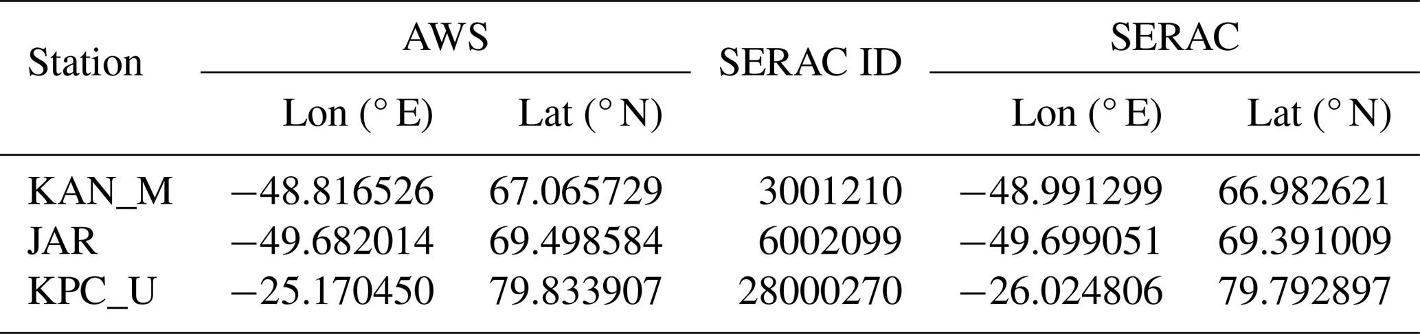
We use AWS data from the melt periods to evaluate the seasonal amplitude in the dSEC data product at the following three locations: Stations KAN_M and JAR (West Greenland), and KPC_U (North Greenland) (see Fig. 1 and Table 1). These stations were selected to provide independent point-scale validation across different climatic regimes of the Greenland Ice Sheet and because they are located sufficiently far from the ice-sheet margin to minimise potential edge effects associated with spatial interpolation and data coverage in the gridded dSEC product.

2.5 SEC time series from laser altimetry-based SERAC and SERAC-FDM fusion

To further evaluate the seasonal amplitude of the dSEC data product, we compare it with the SERAC elevation change time series (Schenk and Csatho , 2012; Csatho et al., 2014; Schenk et al., 2014). SERAC provides localized, high-temporal-resolution elevation-change time series that complement the ATL15 and OIB validations by enabling assessment of seasonal and short-term variability. The SERAC time series are constructed for the locations of the three AWS stations (Table 1).

Table 1 Coordinates of the AWS stations and their corresponding SERAC sites.

The SERAC timeseries is constructed based on a 10 d SEC time series derived from fusing laser altimetry-based SEC time series with firn height change estimations. First the irregularly sampled SEC time series are reconstructed using the SERAC method. The SERAC time series is based on data from all NASA’s airborne and satellite laser altimetry missions and includes observations from the Airborne Topographic Mapping system (ATM), the Land, Vegetation, and Ice Sensor (LVIS) airborne sensors (MacGregor et al., 2021), the Ice Cloud and land Elevation (ICESat, Zwally et al., 2002) and ICESat-2 satellites (Markus et al., 2017). SERAC reconstructs the time series of SEC by simultaneously fitting 1 km² polynomial surface patches and modeling the elevation change at their centroids using all the laser altimetry measurements within the surface patches. The locations of the time series are primarily determined by ICESat ground track crossovers and ICESat’s overlaps with ATM or LVIS to obtain long-term elevation change. Over the Greenland Ice Sheet, SERAC provides over 54 000 time series with irregular temporal sampling determined by the spatiotemporal distribution of the laser altimetry data.

The 10 d resolution SEC time series that we use for validation is calculated as follows. We removed the Glacial Isostatic Adjustment (GIA) uplift rate (Adhikari et al., 2021; Milne et al., 2018) and firn height change from the SERAC SEC time series using the nearest neighbor in space and time to determine the ice thickness change due to ice dynamics. Firn height change, which represents the SEC due to all surface processes, such as precipitation, melt, and firn compaction, is modeled by the Firn Densification Models (FDMs). We use the FDM: Glacier Energy and Mass Balance firn model (GEMB) (Gardner et al., 2023). We estimated the 10 d high temporal resolution time series from the relatively smooth discrete dynamic thickness change time series using the Approximation by Localized Penalized Spline (ALPS) method (Shekhar et al., 2021). By combining the interpolated dynamic thickness change time series with the GIA correction and firn height change estimations, we derived high-temporal-resolution SEC time series at the location of the SERAC time series based on the method by Shekhar et al. (2021).

The seasonal elevation changes in this SERAC-FDM fusion product are well constrained by laser altimetry measurements when sampled seasonally. However, during years with few or no laser altimetry measurements, the seasonal signal is primarily determined by firn height change estimations from FDMs. In this case, seasonality can vary depending on the FDMs selected, and seasonal ice thickness changes due to, e.g., ice dynamics in tidewater glaciers may be missed.

2.5.1 Intercomparison SEC products

To place the dSEC product in the context of existing Greenland-wide surface elevation change (SEC) datasets, we compare it with three independent SEC products: the ICESat-2 ATL15 surface elevation change product (Smith et al., 2022) which is described in detail in Sect. 2.2, the monthly SEC product of Zhang et al. (2022), and the monthly SEC product of Khan et al. (2025).

The SEC product of Khan et al. (2025) provides monthly elevation change rates on a 1 km polar stereographic grid covering the Greenland Ice Sheet. Monthly rates were integrated to cumulative elevation change and subsequently aggregated to the common 5 km grid.

The SEC product of Zhang et al. (2022) provides monthly surface elevation changes at 5 km resolution derived from radar satellite altimetry observations. Since this product is already distributed at a spatial resolution comparable to the dSEC product, only reprojection and spatial matching to the common analysis grid were required.

For all intercomparisons, the products were transformed to a common 5 km polar stereographic grid (EPSG:3413) and restricted to a common ice mask. Temporal consistency was ensured by selecting the nearest available observations corresponding to the ATL15 reference epochs. Product agreement was subsequently evaluated using representative point-scale time series, trend differences, seasonal-amplitude differences, and statistical metrics relative to ATL15. The results of these comparisons are presented in Sect. 4 and in Figs. S2–S4 in the Supplement.

3 State-Space Model

To model the ice surface elevation as a function of time and space, we employ our model 3D-ECM, a data-driven SSM designed to estimate monthly elevation change fields. We define a target grid of 5 km resolution. CryoSat-2 POCA ice surface elevations are extracted using the GrIS ice mask from IMBIE Team (2020), and use elevations relative to the ArcticDEM Mosaic V 4.1 (Porter et al., 2023). The model thus estimates anomalies relative to this DEM rather than absolute surface heights.

Because CryoSat-2 POCA elevation anomalies are irregular in space and time, we adopt a framework that jointly models spatial and temporal correlations to reconstruct coherent surface elevation anomaly fields. This is done via a state-space approach, in which the evolution of surface height in space and time is represented as a set of hidden states that are indirectly observed through noisy satellite elevation measurements. In this framework, the hidden states correspond to the true, but unobservable, surface height anomalies on a regular grid. The observations are the CryoSat-2 Level-2 POCA elevation anomalies relative to ArcticDEM. By linking the hidden and observed components through probabilistic relationships, a State-space model provides a statistical framework that separates measurement noise from true elevation changes.

The large amount of satellite data requires a computationally efficient approach to reconstruct the spatial-temporal field of surface elevation anomalies H^true. To do this, we apply a Gaussian Markov Random Field (GMRF; Rue and Held, 2005). A GMRF is a multivariate Gaussian random field in which the probability of each location is conditionally dependent only on its neighbors, leading to a sparse representation of the precision (inverse covariance) matrix. This is computationally efficient compared to a Gaussian Process (GP) model, in which each location is correlated with every other through a dense covariance matrix that requires costly matrix inversion. Instead, sparsity in the GMRF allows operations to scale almost linearly with the number of grid cells, whereas GP models typically scale cubically with data size. The use of Gaussian Markov Random Fields for spatial modelling follows established geostatistical approaches for representing spatially correlated fields while maintaining computational efficiency (Lindgren et al., 2011). Similar statistical frameworks have been used to reconstruct glacier elevation change from satellite observations, where spatially and temporally correlated signals must be inferred from irregularly sampled measurements (Hugonnet et al., 2021).

To model the ice surface elevation anomalies as a function of time and space, we define a 3-dimensional regular grid. In the spatial dimension, we use a target grid with a 5 km resolution in a polar stereographic projection (EPSG:3413) covering the Greenland Ice Sheet. In the temporal dimension, a monthly resolution is selected. The 5 km spatial resolution and monthly temporal resolution represent a compromise between resolving spatial and seasonal variability and ensuring sufficient data density for spatio-temporal reconstruction given the CryoSat-2 sampling that has a 369 d repeat cycle and a 30 d subcycle (Bouzinac, 2019). For computational efficiency, the model is applied to overlapping spatial tiles that are processed independently. The overlap is introduced through a 15 km padding region, which provides additional observational context near tile boundaries and reduces edge effects in the state-space estimation. Following processing, only the central region of each tile is retained, while results within the padding zone are discarded. Consequently, each 5 km grid cell is represented by a single tile estimate and no averaging between overlapping tiles is required.

Here, we assume that an observation of ice elevation anomaly $H_i^{\mathrm{obs}}$ is a function of space (x,y) and time t is represented by the following expression.

$$\begin{array}{}\text{(1)}& \begin{array}{rl}{H}_i^{\mathrm{obs}}\left(x,y,t\right)& =H_i^{\mathrm{model}}\left(x,y,t\right)\\ & +{\mathit{ϵ}}_i\left(x,y,t\right),{\mathit{ϵ}}_i\sim N\left(\mathrm{0},{\mathit{\sigma }}_{\mathrm{obs}}^{\mathrm{2}}\right),\end{array}\end{array}$$

where $H_i^{\mathrm{model}}$ is the true unobserved elevation anomaly, and ϵ_i represents the observational error, which here is assumed to be Gaussian with the standard deviation σ_obs. The modeled elevation anomaly is represented by a Gaussian Markov random field consisting of a spatial and temporal component with a mean and covariance given as

$$\begin{array}{}\text{(2)}& H^{\mathrm{model}}\left(x,y,t\right)\sim N(\mathit{\mu },{\mathit{\sigma }}_p^{\mathrm{2}}{\left({\mathbf{Q}}_{\mathrm{1}}\otimes {\mathbf{Q}}_{\mathrm{2}}\right)}^{-\mathrm{1}}).\end{array}$$

Here, Q₁ and Q₂ are the precision matrices that define the neighbor structure related to the spatial and temporal parts of the GMRF. The spatial part of the precision matrix is defined as

$$\begin{array}{}\text{(3)}& {\mathbf{Q}}_{\mathrm{1}}=\mathit{\varphi }\cdot {\mathbf{Q}}_{\mathrm{0}}+\mathbf{I},\end{array}$$

where ϕ is a model parameter controlling the spatial correlation, I is the identity matrix, and Q₀ defines the neighborhood structure, which is described as

$$\begin{array}{}\text{(4)}& {\mathbf{Q}}_{\mathrm{0}}\left(i,j\right)=\left\{\begin{array}{ll}\text{number of neighbors of node}i,& \text{if}i=j,\\ -\mathrm{1},& \text{if}i\sim j,\\ \mathrm{0},& \text{otherwise}.\end{array}\right.\end{array}$$

In our framework, the neighborhood structure is built with a 4-nearest-neighbor structure (each grid cell connects to its north, south, east, and west neighbors). The notation i ∼ j indicates that the grid cells i and j share an edge (are directly adjacent to that 4-neighborhood). The precision matrix Q₂ related to the autoregressive process of order 1 is defined as

$$\begin{array}{}\text{(5)}& {\mathbf{Q}}_{\mathrm{2}}=\left(\begin{array}{lrrrr}\mathrm{1}& -\mathit{\rho }& & & \\ -\mathit{\rho }& \mathrm{1}+{\mathit{\rho }}^{\mathrm{2}}& \mathrm{\ddots }& & \\ & \mathrm{\ddots }& \mathrm{\ddots }& \mathrm{\ddots }& \\ & & \mathrm{\ddots }& \mathrm{1}+{\mathit{\rho }}^{\mathrm{2}}& -\mathit{\rho }\\ & & & -\mathit{\rho }& \mathrm{1}\end{array}\right)\end{array}$$

where ρ is a parameter that controls the temporal correlation assumed to be between −1 and 1 to ensure that the process is stationary. In summary, the full model parameters vector $\mathit{\theta }=({\mathit{\sigma }}_{\mathrm{obs}},{\mathit{\sigma }}_p,\mathit{\mu },\mathit{\varphi },\mathit{\rho }$) and the hidden states H^true are estimated by the joint likelihood function

$$\begin{array}{}\text{(6)}& L\left(H^{\mathrm{obs}},H^{\mathrm{true}},\mathit{\theta }\right)=L\left(H^{\mathrm{obs}},\mathit{\theta }\right)L\left(H^{\mathrm{true}}\right)\end{array}$$

As the hidden states H^true are unobserved, the joint likelihood cannot be calculated directly. Instead, we form the marginal likelihood function, which is only dependent on the fixed model parameters and the observation.

$$\begin{array}{}\text{(7)}& L_{\mathrm{M}}\left(H^{\mathrm{obs}},\mathit{\theta }\right)=\int L\left(H^{\mathrm{obs}},H^{\mathrm{true}},\mathit{\theta }\right)\mathrm{d}{H}^{\mathrm{true}}.\end{array}$$

The 3D model of ice elevation anomalies is implemented in the open source software R using the Template Model Builder (RTMB) (Kristensen et al., 2016). In RTMB, the marginal likelihood is derived via the Laplace approximation. In short, this is a second-order Taylor approximation of the logarithm of the function to be integrated around the optimum. In practice, this will change an integral into an optimization problem.

The GMRF captures both the spatial coherence and temporal evolution of elevation changes. This joint formulation allows efficient and realistic reconstruction of SEC over the Greenland Ice Sheet, even in areas with irregularly distributed data. RTMB also reports the model uncertainty, which is approximated via the generalized delta-method, and the variance is expressed as

$$\begin{array}{}\text{(8)}& \text{var}\left({\widehat{H}}^{\mathrm{true}}\right)={\mathbf{H}}_{\mathrm{2}}^{-\mathrm{1}}+(\mathrm{\nabla }{\widehat{H}}^{\mathrm{true}}\left(\mathit{\theta }\right){)}^{\mathrm{t}}{\mathbf{H}}_{\mathrm{1}}^{-\mathrm{1}}\mathrm{\nabla }{\widehat{H}}^{\mathrm{true}}\end{array}$$

Here H₂ is the block of full Hessian matrix related to the hidden states, H₁ is the Hessian matrix related to the parameters, and $\mathrm{\nabla }{\widehat{H}}^{\mathrm{true}}$ are the gradients of the hidden states with respect to the model parameters θ (Kristensen et al., 2016). The generalized delta-method approximates the uncertainty of the reconstructed field by propagating parameter uncertainty through a first-order Taylor expansion around the optimum.

To reduce residual high-frequency variability not fully captured by the statistical model and enhance the spatiotemporal coherence of the SEC dataset, we subsequently apply a two-step postprocessing of the monthly dSEC gridded fields. The trends of both the raw (pre-smoothing) and the smoothed dSEC grids will be evaluated separately in Sect. 4.1.1. First, each monthly elevation map is smoothed with a median spatial filter with a window size of 5 × 5 gridcell to suppress small-scale noise while retaining the larger-scale elevation signals. Secondly, for temporal consistency, a Savitzky-Golay filter (Gallagher, 2020) is applied along the time axis. For the seasonal component, we use a 17-month window, which is longer than the annual cycle and therefore provides a smoothed and damped representation of the seasonal signal while removing month-scale irregularities. To extract the multi-year trend, we use a 41-month window, which effectively isolates the long-term trends of SEC. This procedure efficiently suppresses noise and outlier-driven seasonal spikes, while preserving the large-scale spatial patterns and long-term elevation-change signals.

The grid-cell uncertainties are first obtained from the state-space model as posterior standard deviations derived from the RTMB Hessian. These uncertainties are then propagated through the full post-processing chain using a Monte Carlo approach, in which Gaussian perturbations consistent with the model estimated variance are added to the elevation fields and passed through the same spatial and temporal post-processing chain. The final uncertainty at each grid cell and epoch is computed as the standard deviation across ensemble realizations of the filtered product.

For regional averages of SEC (e.g., Greenland-wide, interior, and ablation-zone means shown in Fig. 3), grid-cell values were combined using a latitude-dependent area-weighted mean, with weights proportional to cos (ϕ), where ϕ is the latitude of each grid cell. The uncertainty of each regional mean was propagated from the individual grid-cell uncertainties using standard error propagation for a weighted mean. Spatial correlations between neighbouring grid cells were not explicitly included in this uncertainty propagation, and the resulting regional uncertainties may therefore underestimate the true uncertainty.

4 Results

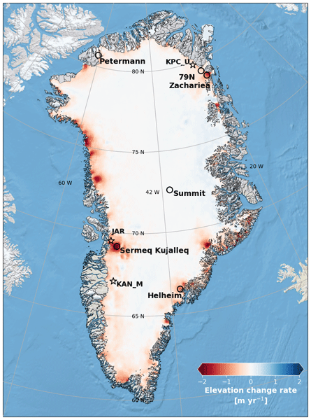
Using the described 3D-ECM model framework, we computed the monthly SECs across the GrIS at a 5 km resolution using radar satellite data from the CryoSat-2 L2 data product. A spatial map of the average SEC from 2011–2025 produced by our 3D-ECM is presented in Fig. 1, with time series of elevation change at selected locations in Fig. 2. Widespread thinning is observed along the margins and generally stable or slightly thickening conditions in the ice sheet interior (in the following defined as areas above 1500 m elevation based on ArcticDEM). The average trend in SEC over the entire GrIS is −0.069 ± 0.002 m yr⁻¹, as illustrated in Fig. 3, whereas the trend in the ablation zone (defined as areas below 1500 m elevation based on ArcticDEM) is −0.314 ± 0.009 m yr⁻¹. The shaded regions in Fig. 3 represent the uncertainty of the mean elevation change at each timestep, derived from the grid-cell uncertainties estimated by the state-space model and propagated through the spatial averaging. As the time series represent elevation anomalies at each timestep rather than cumulative changes, the uncertainties do not accumulate over time.

To assess regional variability and temporal evolution, we extracted time series from six locations across the Greenland Ice Sheet (Panels A–F in Fig. 2). These sites are representative of dynamically active outlet glaciers: Petermann, Nioghalvfjerdsbræ (79° N Glacier; hereafter 79° N), Zachariae, Sermeq Kujalleq, and Helheim, as well as a site representative of the relatively stable interior region at Summit Station.

The time series are extracted from single grid cells, with shaded areas in Fig. 2 representing the uncertainty estimated from the 3D-ECM model. Derived from the smoothed CryoSat-2 dSEC product, they reveal spatially varying elevation change patterns from 2011 to 2025. The Summit site, located within the interior zone (> 1500 m elevation), shows a modest thickening trend of 0.017 ± 0.001 m yr⁻¹ over the 14-year period, close to the negligible average trend for the interior ice sheet of −0.014 ± 0.002 m yr⁻¹.

All marginal sites exhibit pronounced thinning. Sermeq Kujalleq experiences the strongest thinning of −1.7 ± 0.074 m yr⁻¹, exceeding the mean trend of the ablation zone (−0.314 ± 0.009 m yr⁻¹). The maximum thinning at Sermeq Kujalleq occurs during the early part of the record, between 2011 and 2018.

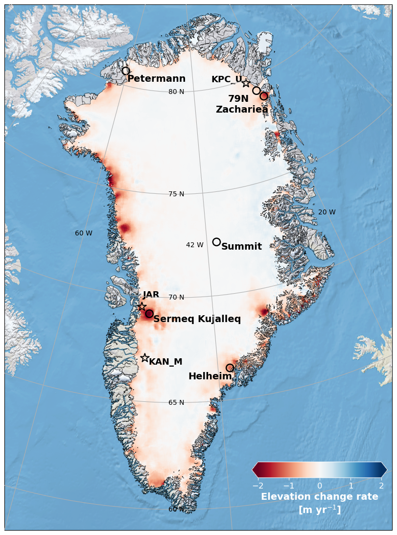
Figure 1 Spatial distribution of surface elevation change rate (m yr⁻¹) over the Greenland Ice Sheet for the period 2011–2025 derived from CryoSat-2 data © ESA. Black circles indicate the locations where elevation-change time series are extracted (shown in Fig. 2). Stars mark the positions of PROMICE automatic weather stations used for comparison later.

Figure 2 Time series of SEC at six selected locations across the Greenland Ice Sheet derived from the smoothed CryoSat-2 dSEC product. Fig. 2 (A)–(F) show time series for Sermeq Kujalleq, Petermann, Summit, 79N, Zachariae, and Helheim, respectively. Shaded envelopes indicate propagated 1σ uncertainty.

Figure 3 The average time series of SEC across the entire GrIS (in blue), the interior (here defined as areas above 1500 m of elevation based on ArcticDEM; in purple), and for the marginal zone (areas below 1500 m of elevation; in red). Shaded envelopes indicate propagated 1σ uncertainty.

The CryoSat-2 Level-2 altimetry data contain a spatial data gap over the fast-flowing part of Sermeq Kujalleq, where steep topography and complex radar scattering hinder reliable surface elevation retrievals, as seen in Fig. 4, which provides a detailed example for the Sermeq Kujalleq, showing dSEC for three grid cells located inside and outside the persistent data gap for CryoSat-2 data. Grid cells B and C are located within the persistent CryoSat-2 data gap, while A is situated further inland in an area with higher data density. The associated uncertainties differ among the three points, reflecting the varying data density, with higher uncertainties in areas of sparse CryoSat-2 coverage and lower uncertainties inland where data are more abundant. Because CryoSat-2 data density in this region is relatively consistent over time per grid cell, and the posterior variances are propagated through the same spatial and temporal filtering as the model output, the resulting uncertainties remain relatively constant between months. These time series reveal distinct seasonal cycles and interannual variability, demonstrating the ability of this approach to resolve fine-scale temporal changes in rapidly evolving glacier systems.

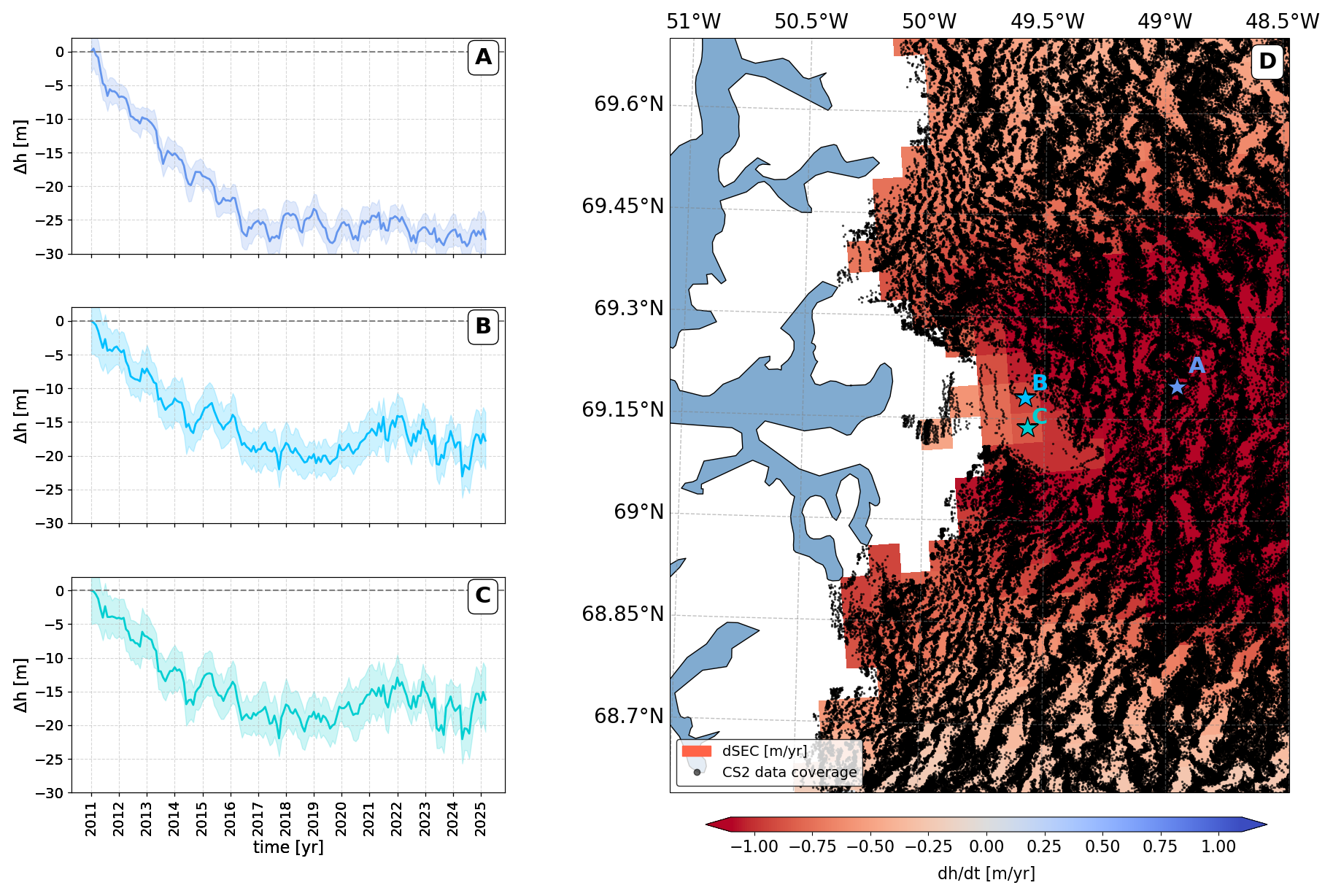
Figure 4 dSEC on Sermeq Kujalleq. Panels (A)–(C) show time series of dSEC for three selected grid cells (stars), with shaded envelopes indicating propagated model 3σ uncertainty . Panel (D) shows the spatial distribution of CryoSat-2 data © ESA (black dots) and the corresponding dSEC $\mathrm{d}h/\mathrm{d}t$ map for 2011–2025.

4.1 Validation and Intercomparison

To evaluate the accuracy and reliability of the CryoSat-2 derived dSEC product over the Greenland Ice Sheet, we performed a validation and intercomparison using satellite, airborne, in situ, and published community SEC datasets. The assessment is carried out in three stages. First, the trends in the dSEC product are validated against independent measurements from NASA's Operation IceBridge (OIB) and the ICESat-2 ATL15 data product. Second, the dSEC product is quantitatively intercompared with existing published Greenland SEC products to place the results in the context of current community datasets. Third, seasonal variability is evaluated using in situ observations from Automatic Weather Stations (AWS) and elevation-change estimates from the altimetry-based SERAC time series.

4.1.1 Validation of trend

To validate the long-term trend of the dSEC product, we compare our dSEC estimates against ICESat-2 ATL15 5 km re-gridded SEC data and OIB airborne altimetry measurements. These independent datasets provide complementary spatial and temporal perspectives, allowing for a robust assessment of the performance of our satellite-derived dSEC product. The validation is conducted across multiple time periods, enabling us to investigate consistency and potential biases over time. We analyze both the original (raw) and post-processed (smoothed) versions of the dSEC product to assess the impact of the applied noise-reduction techniques on the agreement with reference datasets.

To evaluate the overall agreement between the dSEC product and ICESat-2 ATL15. To ensure temporal consistency, the dSEC height time series was evaluated at the same epochs as the ICESat-2 ATL15 product. Because ATL15 lag-8 represents 24-month elevation-change rates centered on each observation epoch, comparable 24-month $\mathrm{d}h/\mathrm{d}t$ estimates were derived from the dSEC height time series centered on the same ATL15 timestamps. We then compared the distribution of elevation-change differences (dSEC minus ICESat-2 ATL15) for both the raw and smoothed versions (i.e., before and after the post-processing step) of the dSEC dataset (Table 2 and Fig. 5). The smoothed dSEC product displays a narrower distribution of differences than the raw version, reducing the standard deviation (STD) from 0.96 to 0.54 m yr⁻¹ and the median absolute difference (MAD) from 0.24 to 0.1 m yr⁻¹. As shown, in the Table 2 the STD of the raw versus smoothed model output was reduced by approximately 44 %, and the MAD by around 56 %, while the mean difference remained unchanged at 0.11 m yr⁻¹. The median differences are close to zero in both cases (−0.01 for raw and −0.02 m yr⁻¹ for smoothed), suggesting minimal systematic bias. Across all selected annual periods (Table 2), these results demonstrate that the applied spatio-temporal smoothing effectively reduces high-frequency noise while preserving the underlying elevation change signal.

Table 2 Summary statistics of the difference between dSEC and ICESat-2 ATL15 (dSEC-ATL15) for selected ATL15 epochs. ATL15 lag-8 provides 24-month elevation-change rates ($\mathrm{d}h/\mathrm{d}t$) centered on each observation epoch. Comparable 24-month $\mathrm{d}h/\mathrm{d}t$ estimates were derived from the dSEC height time series centered on the same epochs. The ranges listed in the first column indicate the span of ATL15 midpoint epochs included in each comparison. Each epoch includes results for both original (Raw) and post-processed (Smoothed) dSEC products. All values are in m yr⁻¹. The final column shows the percentage reduction in standard deviation (STD) after smoothing.

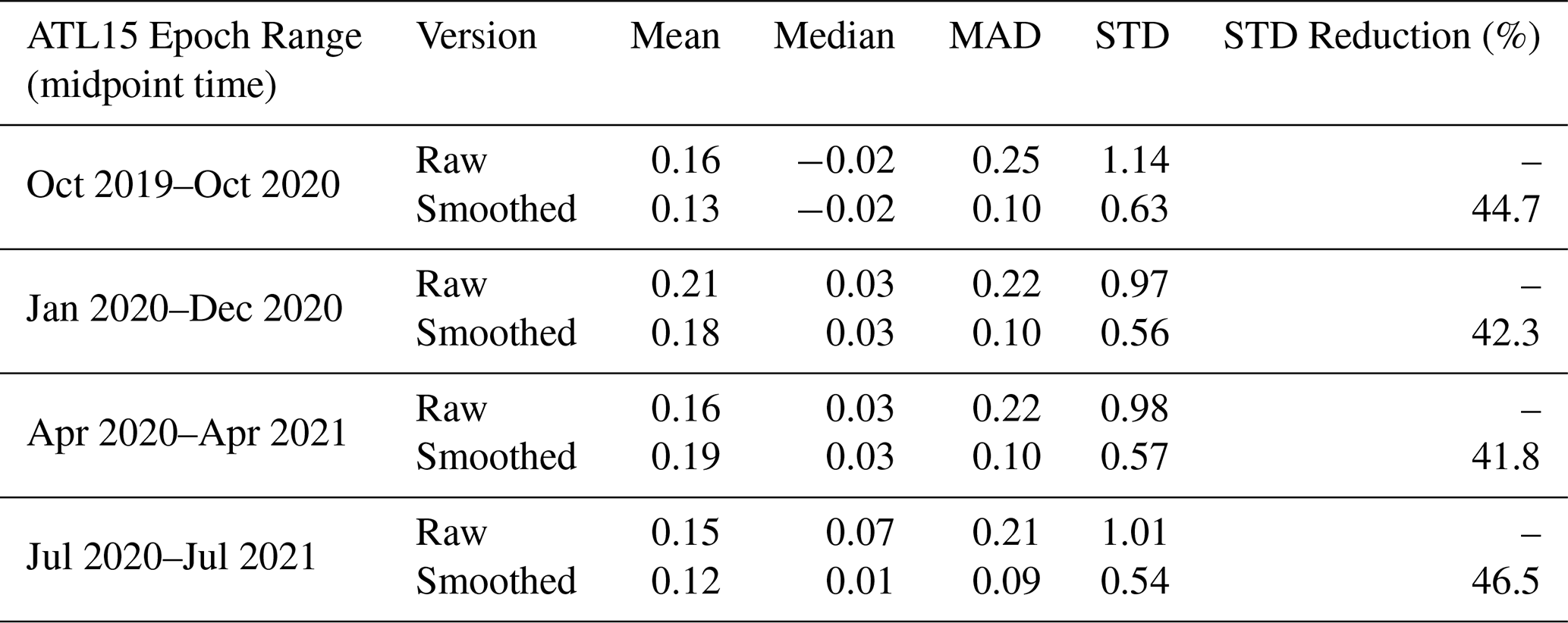
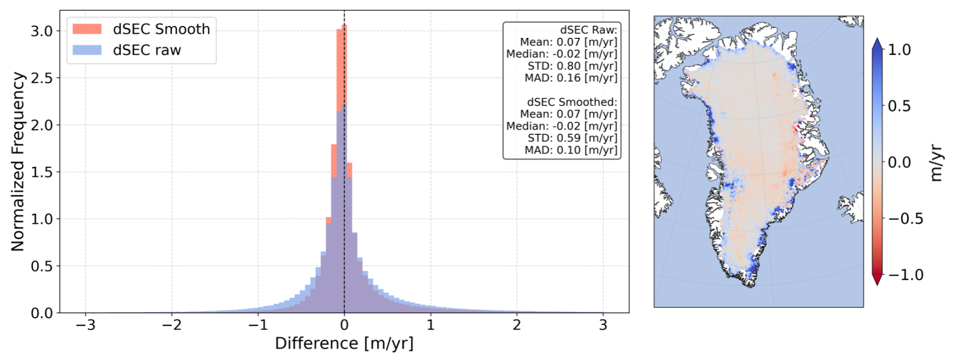
Figure 5 Left: Histogram comparing the differences between the dSEC product (raw and smoothed) with the ICESat-2 ATL15 data © NASA over the GrIS. Right: Difference between the two products (smoothed dSEC-ATL15) over the overlapping ATL15 period (2018–2025).

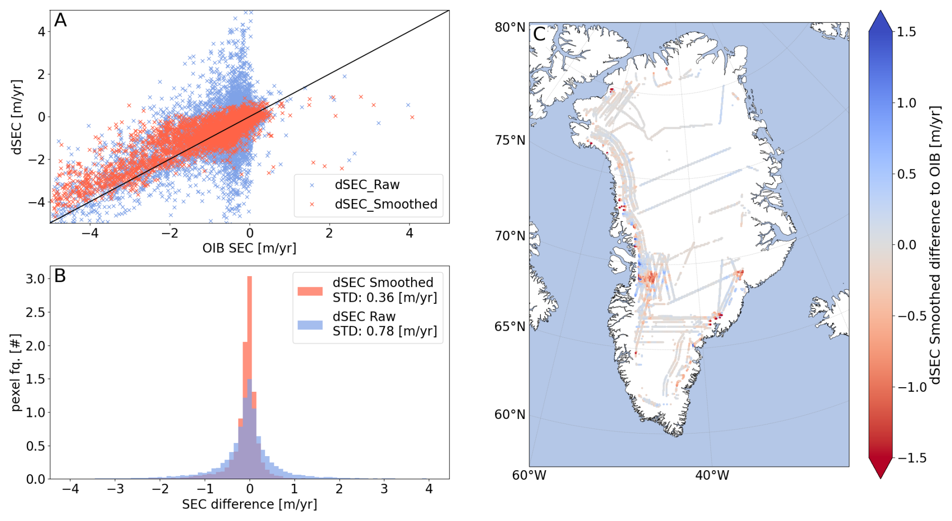
Figure 6 Comparison of dSEC derived from CryoSat-2 data © ESA with Operation IceBridge altimetry data © NASA from 2011–2016. (A) Scatterplot comparing both the raw (blue) and spatially smoothed (red) dSEC data to OIB SEC values. The 1 : 1 line is shown in black. (B) Histogram of the elevation change differences (dSEC-OIB) for raw (blue) and smoothed (red) data. (C) Spatial distribution of the difference between smoothed dSEC and OIB SEC, colored by magnitude of difference (in m yr⁻¹).

To further assess the accuracy of the satellite-derived dSEC estimates, we also validate the data set against multiple campaigns of OIB airborne altimetry data. Figure 6A shows a point-by-point comparison between OIB and dSEC values for the raw and smoothed dSEC data set, respectively. After smoothing, large discrepancies are reduced, and the product aligns more closely with the OIB measurements. This improvement is also visible from panel B, where the histogram of the differences in elevation change reveals a narrower distribution for the smoothed data: the STD of the difference between dSEC and OIB SEC is reduced by 50 % from 0.78 in the raw product to 0.37 m yr⁻¹ after smoothing. Panel C maps the spatial distribution of dSEC-OIB differences across the GrIS, illustrating that the largest residuals are predominantly located in the vicinity of the Sermeq Kujalleq Ice Stream. Nevertheless, the remaining differences tend to increase with increasing elevation-change magnitude, where dSEC generally exhibits smaller changes than those observed by OIB. This behaviour likely reflects a combination of the spatial smoothing applied within the 3D-ECM framework and differences in spatial sampling. While OIB measurements can capture highly localized elevation changes along individual flight tracks, the gridded dSEC product represents an area-averaged estimate at 5 km resolution and may therefore attenuate extreme thinning and thickening signals.

The overall results confirm that the spatio-temporal filtering applied to the satellite elevation time series ensures an enhanced agreement with independent satellite and airborne validation data, particularly by reducing noise. In the following, the post-processed version of the dSEC data set will be used.

4.1.2 Intercomparison with community SEC products

In this section we intercompare our dSEC product with two published, Greenland-wide SEC products, the monthly 5 km grid SEC product from Zhang et al. (2022) and the smoothed monthly Greenland 1 km grid SEC product of Khan et al. (2025). While this intercomparison is not an independent validation, it provides important context for how our dSEC product performs relative to other community products.

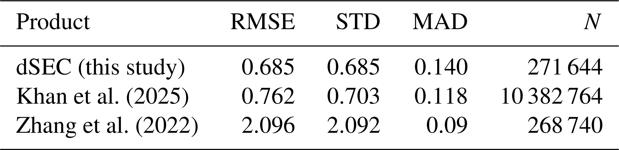
To quantify relative performance against an independent reference, we evaluate each SEC product against ICESat-2 ATL15 over the common spatio-temporal domain. We summarize the distribution of differences with commonly used metrics; the root mean square error (RMSE), STD, and MAD.

Table 3 shows that our dSEC product achieves the lowest overall misfit relative to ATL15 among the evaluated SEC products. In particular, dSEC exhibits lower RMSE and reduced spread of differences compared to both Khan et al. (2025) and Zhang et al. (2022). Together, these results indicate that the proposed 3D-ECM framework yields elevation-change estimates that are comparable to, and in this evaluation show improved agreement with, independent ICESat-2 laser altimetry.

Table 3 Intercomparison of SEC products against ICESat-2 ATL15 over the common spatio-temporal domain. Metrics summarize the distribution of differences (product minus ATL15).

To further investigate product agreement, additional spatial and temporal comparisons are provided in the Supplement. Figure S2 presents maps of mean elevation-change rates and trend differences relative to dSEC, while Fig. S3 compares the spatial distribution of seasonal amplitudes. Representative time series from six locations across Greenland are shown in Fig. S4. Overall, the products exhibit similar large-scale patterns of elevation change, including widespread thinning along major outlet glaciers and smaller changes in the interior ice sheet. The largest differences occur in the marginal regions with rapid dynamic change.

Taken together, these comparisons demonstrate that the dSEC product is broadly consistent with existing Greenland-wide SEC datasets while showing improved agreement with the independent ATL15 reference data.

4.1.3 Evaluation of seasonal variability using AWS and SERAC observations

We evaluate the seasonal amplitude of the dSEC product at three sites (Table 1) using AWS-derived daily relative surface height (Fausto et al., 2021; Vandecrux et al., 2024) and SERAC-FDM fusion (Csatho et al., 2014; Shekhar et al., 2021). By comparing the amplitude of the melt-season signal in our satellite-derived dSEC data with that from AWS time series, we are able to assess the consistency of the dSEC product against independent measurements. The three AWS stations were selected to provide independent point-scale validation across different climatic regimes of the Greenland Ice Sheet. However, these sites are not intended to be representative of the full spatial variability of the dSEC product, and the AWS comparison should therefore be interpreted as a local validation of seasonal variability rather than a Greenland-wide assessment.

Comparisons of the dSEC and SERAC time series are shown in the upper panels of Fig. 7. To assess average short-term variability, we compute the average seasonal cycles for these three locations. The mean seasonal cycles were computed from the linearly detrended time series by grouping observations by calendar month and calculating the mean value for each month over the common period 2011–2024. The shaded envelopes represent the ±1σ variability of the detrended monthly values across all years. These mean seasonal cycles are shown in the lower panels of Fig. 7. Across sites, dSEC generally reproduces the phase of seasonal variability observed in both SERAC and AWS, and the amplitude differences between sites are evident. For example, KAN_M shows a pronounced seasonal cycle in all three datasets.

We further quantify the temporal agreement between the three data sets during the period 2011–2024 (the overlap between CryoSat-2 and SERAC) by computing Pearson correlation coefficients between linearly interpolated, detrended dSEC time series and those from AWS and SERAC (Table 4). Additional AWS correlation analyses are provided in Fig. S5.

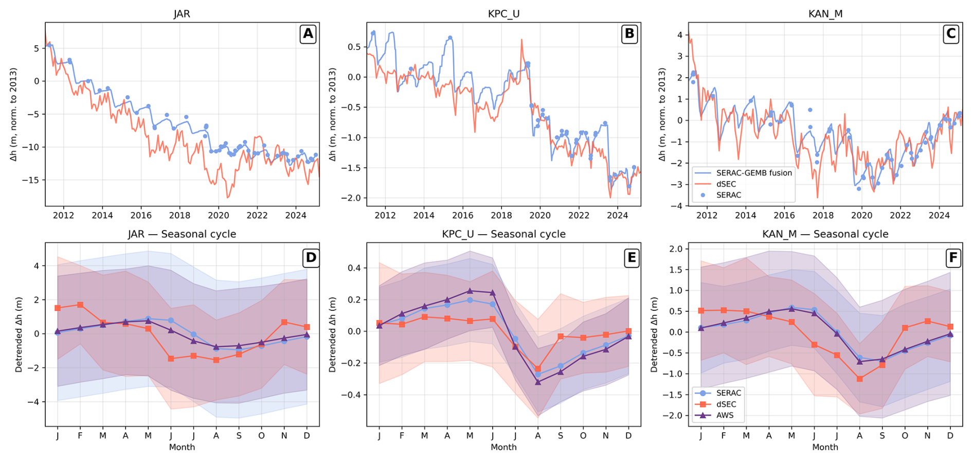
Figure 7 (A–C): Elevation change at three AWS validation sites (JAR, KPC_U, KAN_M). Time series of elevation change from SERAC (blue dots), dSEC (orange), and GEMB (blue), aligned to zero at the start of the CryoSat-2 period (2011) for direct comparison. (D–F) Average seasonal cycles of detrended elevation change for the same stations, based on dSEC (orange), AWS (purple), and SERAC (blue) data, with shaded envelopes indicating ±1σ statistical variability within each calendar month. Note the different scale on the y-axis. The locations of the AWS stations are shown in Fig. 1.

Table 4 Pearson correlation coefficients (r) between linearly detrended time series from the dSEC product, SERAC and AWS at each station. Correlations are computed over 2011–2024 after linear detrending and interpolation to a common temporal grid.

5 Discussion

Our results illustrate how our data-driven 3D-ECM framework can advance the monitoring of ice-sheet surface elevation from satellite radar altimetry. By integrating radar altimetry observations with a spatio-temporal statistical model, we obtain continuous, monthly estimates of dSEC over the Greenland Ice Sheet, including regions where satellite sampling is sparse or irregular. The combination of a GMRF representation of spatial dependence with an autoregressive temporal component allows the model to isolate meaningful elevation-change signals, while additional post-processing of the radar data further reduces high-frequency noise.

This capability has important implications for interpreting both seasonal variability and interannual trends in ice sheet surface elevation change. It also highlights the potential to unify data from different altimetry missions and sensor types. Although here we focus on CryoSat-2, the same framework could be applied to past and future radar altimeters, enabling more consistent long-term monitoring across satellite generations. The framework can also be applied to laser altimetry missions such as ICESat-2, although in this study ICESat-2 is used solely as an independent validation dataset.

Uncertainty patterns in the dSEC product highlight the dependence of model performance on data density. Figure 4 shows how the uncertainty estimates of the dSEC product are higher in grid cells B (7.1 m ± 1.3 m) and C (7.6 m ± 0.34 m), located within the CryoSat-2 data gap, compared to A (4.8 ± 1.6 m), which is situated in an area with a higher data density. Here, the first value denotes the average uncertainty across the time series, while the ± value represents the temporal variability (standard deviation) of the uncertainty estimate. As expected, model uncertainty, and therefore also propagated uncertainties, increases with distance to available data points; nevertheless, the 3D-ECM reconstructs coherent temporal patterns even in poorly sampled regions. For example, cells B and C capture a pronounced thinning from 2011–2016, consistent with previous studies (Khazendar et al., 2019; Joughin et al., 2020; Hansen et al., 2021), followed by reduced thinning, and reproduce the surface build-up observed between 2019 and 2021 in the trough of the Sermeq Kujalleq Ice Stream (Hansen et al., 2021), despite lying within an almost persistent data gap.

The monthly dSEC product is based on satellite radar altimetry and inherits its sensitivity to changes in surface scattering properties, i.e., the way the radar signal interacts with the surface before it is reflected to the satellite. For instance, an increase in surface roughness will broaden and flatten the returned signal (the waveform), making the identification of the surface reflection more difficult in that waveform (Ridley et al., 1988; Rémy et al., 2009; Ricker et al., 2014). Over polar snow and firn (cold, dry conditions), CryoSat-2’s Ku-band (13.6 GHz) radar typically penetrates up to about 1–2 m (Armitage et al., 2014). Variations in volume scattering within that depth range (changes of snow density or grain size) can affect the returned waveform and distort surface elevation estimates (Aublanc et al., 2021; Fredensborg et al., 2024). Likewise, the appearance of an ice layer within that penetration depth may cause a waveform peak at that horizon, which is then interpreted as the surface (Nilsson et al., 2016). Such effects introduce elevation biases that cannot be fully eliminated by statistical smoothing. Consequently, interpretation of dSEC trends must consider changing surface conditions, particularly in regions experiencing melt, refreezing, or firn densification changes.

Independent validation against ICESat-2 ATL15 and OIB shows that post-processing improves quantitative agreement. Compared to the raw reconstruction, the smoothed dSEC product reduces the annual standard deviation of differences by 40 %–45 % and lowers the median absolute deviation, indicating more stable and spatially coherent elevation-change estimates.

The intercomparison with published SEC products further contextualizes these results. Relative to existing monthly SEC products, the 3D-ECM framework shows reduced spread of differences against ICESat-2 ATL15, suggesting that the joint spatio-temporal modeling provides a more coherent reconstruction of elevation change fields. Additional spatial and temporal comparisons presented in Figs. S2–S4 support this interpretation. The largest trend differences are concentrated in dynamically active outlet-glacier regions, whereas agreement is generally stronger across the interior ice sheet.

Station-specific comparisons with AWS records and the altimetry-based SERAC product further illustrate how local glaciological conditions affect dSEC interpretation. At JAR (close to Sermeq Kujalleq), dSEC correlates moderately with AWS (r= 0.58) and more strongly with SERAC (r= 0.76). The weaker agreement with AWS likely reflects dynamic ice-thickness changes near the fast-flowing outlet glacier Sermeq Kujalleq that are not captured by surface instruments, consistent with observations of strong velocity variability in this region (Joughin et al., 2014; Mouginot et al., 2019). In contrast, KPC_U is located on an ice lobe north of the Northeast Greenland Ice Stream where seasonal dynamics are minimal. Here dSEC, AWS, and SERAC show strong agreement (all r> 0.72; AWS-SERAC r= 0.92). KAN_M, in the southwest percolation zone, exhibits high correlation between dSEC and both AWS and SERAC but a lower correlation between AWS and SERAC themselves, consistent with the complex interplay of firn compaction, meltwater infiltration, retention, and refreezing in this region. Notably, both dSEC and SERAC record a shift toward more positive trends around 2020 at KAN_M (Fig. 7), suggesting that both datasets capture the same seasonal evolution despite these challenging surface processes.

Taken together, these comparisons show that the dSEC product agrees well with both the AWS records and the altimetry-based SERAC product, indicating that the 3D-ECM framework captures physically meaningful elevation change signals consistent with independent observations. However, these examples also emphasize that while the 3D-ECM framework successfully extracts coherent elevation change patterns, interpretation at the local scale must account for the diverse physical processes that govern different climatic and glaciological regimes across Greenland.

The 3D-ECM framework integrates radar altimetry observations within a coherent spatio-temporal reconstruction, enabling the generation of spatially and temporally consistent, gap-filled SEC time series across the Greenland Ice Sheet. An advantage of the 3D-ECM framework is its flexibility, which is applicable across multiple satellite missions and enables the production of continuous, gap-filled SEC time series at varying spatial and temporal scales. Importantly, the framework is entirely data-driven: seasonal variability emerges directly from the observations through the joint spatio-temporal estimation, rather than being prescribed using a predefined harmonic (sine-cosine) formulation. In several existing SEC approaches, seasonality is represented using fixed parametric functions that implicitly assume a stationary and symmetric seasonal cycle with constant amplitude and phase, as in Sørensen et al. (2018) and Khan et al. (2025). In contrast, the present framework does not impose a parametric seasonal model, the 3D-ECM framework allows for non-sinusoidal seasonal shapes as well as temporal changes in amplitude and phase. This flexibility is particularly relevant for Greenland, where seasonal elevation changes vary regionally and interannually in response to evolving melt and accumulation conditions. A potential development for future enhancement of the spatial resolution of the dSEC product is the use of swath-processed CryoSat-2 data (Gray et al., 2013; Gourmelen et al., 2018; Andersen et al., 2021) instead of the Level-2 POCA dataset, due to the higher data density of the swath-processed CryoSat-2 data.

To place the reconstructed dSEC fields in the context of existing community datasets, we compared the product against two published community SEC products (Zhang et al., 2022; Khan et al., 2025) using ICESat-2 ATL15 as a reference over the common spatio-temporal domain (Table 3). The comparison shows that the dSEC product yields a lower RMSE relative to ATL15 than the evaluated community products and exhibits a reduced spread of differences compared to Zhang et al. (2022). The relatively small MAD values for all products suggest that the central tendencies of the distributions are similar, while differences in RMSE and standard deviation mainly reflect variations in the spatial and temporal coherence of the reconstructed SEC fields. Overall, this comparison indicates that the spatio-temporal state-space framework produces SEC estimates that are consistent with independent laser altimetry and comparable to, or slightly improved relative to, existing community SEC products.

The 3D-ECM framework relies on several modeling assumptions that should be considered when interpreting the dSEC product. The spatio-temporal structure combines a Gaussian Markov Random Field in space with a first-order autoregressive process in time, imposing local spatial dependence and exponentially decaying temporal correlations. While computationally efficient for ice-sheet-scale reconstruction, this formulation may not fully capture long-range spatial correlations or complex glacier dynamics. Observational errors are assumed to be Gaussian and uncorrelated, although radar altimetry can exhibit spatially and temporally correlated errors that are not explicitly modeled; uncertainties therefore represent posterior uncertainty under the assumed model structure.

The state-space model is designed to reconstruct the dominant spatial and temporal evolution of surface elevation change, but it does not explicitly separate high-frequency variability from the underlying signal. Consequently, short-term fluctuations associated with measurement noise, irregular sampling, or transient processes may remain present in the reconstructed fields. To derive the final monthly dSEC product, an additional post-processing step consisting of spatial median filtering and temporal Savitzky-Golay filtering is therefore applied to suppress high-frequency noise and improve spatial coherence. While this substantially improves agreement with independent validation datasets, it may also smooth some short-term variability.

In the revised framework, uncertainties are propagated through this post-processing using a Monte Carlo approach, such that the reported 1σ uncertainty reflects the fully filtered product. For computational efficiency, the model is implemented in overlapping spatial tiles, which may introduce subtle edge effects. Despite these limitations, the 3D-ECM provides a flexible and computationally efficient framework for reconstructing coherent monthly elevation-change fields from irregularly sampled altimetry observations, balancing model complexity, interpretability, and computational feasibility at ice-sheet scale.

6 Conclusions

We have derived monthly dSEC across the Greenland Ice Sheet for the period 2011–2025 from CryoSat-2 radar altimetry. The state-space model combines a Gaussian Markov Random Field for spatial dependencies with an autoregressive temporal process, allowing seasonality, long-term trends, and abrupt changes to emerge directly from the data without prescribing functional forms. The reference surface was taken from ArcticDEM, and the analysis was restricted to the Greenland Ice Sheet mask defined within the IMBIE framework (IMBIE Team, 2020), excluding peripheral glaciers and ice caps not dynamically connected to the main ice sheet.

The resulting dataset captures both broad spatial patterns and local outlet-glacier variability, while providing consistent point-based time series across the ice sheet. Independent validation confirms the robustness of the approach as comparisons with ICESat-2 ATL15 and NASA Operation IceBridge show strong agreement in long-term trends, with spatio-temporal smoothing reducing spread while maintaining minimal bias. Seasonal amplitudes from AWS and SERAC time series also align closely with the linearly detrended dSEC product, demonstrating that the method resolves both interannual and seasonal variability.

Intercomparison with two published community SEC products further shows that the dSEC reconstruction achieves comparable or lower misfit relative to ICESat-2 ATL15, indicating that the spatio-temporal state-space framework provides consistent SEC estimates relative to existing community datasets.

Beyond the Greenland and CryoSat-2 application, the modeling framework is directly transferable to other altimetry missions and multi-sensor combinations. Its computational efficiency enables long-term monitoring of polar ice sheets and provides a pathway for integrating upcoming missions such as CRISTAL into multi-decadal elevation-change records.

In summary, the presented dSEC dataset delivers monthly, high-resolution, and uncertainty-quantified estimates of SEC across the Greenland ice sheet. The approach provides temporally consistent monthly fields from irregularly sampled radar altimetry observations, support future assessments of ice-sheet mass balance and dynamics and provide a foundation for continuous, multi-mission monitoring of the cryosphere.

Appendix A: Map of Model Uncertainty

Figure A1 shows the spatial distribution of the uncertainty for the monthly dSEC product after spatial and temporal postprocessing. The uncertainty field is derived from the model-based uncertainties produced by the state-space model and subsequently propagated through the same filtering steps applied to the elevation-change field. This ensures that the reported uncertainties represent the effective uncertainty of the final postprocessed product rather than the raw model output.

Higher uncertainties occur in regions with sparse CryoSat-2 coverage, while the interior of the ice sheet exhibits lower uncertainty due to denser and more stable sampling.

In addition, subtle patterns related to tile boundaries can be visible in the uncertainty field. These arise because the model is solved in overlapping spatial tiles for computational efficiency, which can introduce small differences along tile edges.

Figure A1 Spatial distribution of the uncertainty of the dSEC model field. Areas with sparse CryoSat-2 © ESA observations exhibit higher uncertainty, while interior regions with denser coverage show substantially lower uncertainty.