Climatology and Interannual Variations in Arctic Winter Sea Ice Leads in the ICESat-2 Era

Sea ice leads play a key role in polar air-sea heat, moisture, and gas exchanges, ocean heat and salinity variations, and ecosystem processes. However, their small-scale nature challenges efforts to assess spatiotemporal variability on a pan-Arctic basis. Here, we use six years of high spatial resolution surface type (ATL07) and freeboard (ATL10) products from Ice, Cloud, and Land Elevation Satellite-2 (ICESat-2) to characterize Arctic winter sea ice leads. Both products reveal consistent climatological spatial patterns, with lead fractions generally higher near the ice edge and coastal regions, and lower over the central abyssal plains. Lead sizes follow a power-law distribution, with the exponent increasing with size. We identify four distinct features in the temporal evolution of lead fraction over the ICESat-2 era, including a maximum in winter 2020–2021. Increases in lead fraction are primarily driven by changes in the number of larger (> 100 m) leads. Our findings show that ICESat-2 measurements provide robust regional-scale characterization of spatiotemporal variability in winter ice leads, which will in turn better inform their underlying response to, and influence on, Arctic climate.

1 Introduction

Sea ice leads are elongated cracks in sea ice with widths of a few to hundreds of meters and lengths of several to hundreds of kilometers (e.g., Alam, 1997; Miles and Barry, 1998; Marcq and Weiss, 2012; Muchow et al., 2021). They are formed by ice shear and/or divergence driven by winds, ocean currents, internal stress and inertial forces (e.g., Miles and Barry, 1998; Marsan et al., 2004). Despite their overall small areal coverage in the pack ice during the ice growing season (a few percent, e.g., Alam, 1997; Wernecke and Kaleschke, 2015; Tilling et al., 2019), leads play important roles in ocean and atmospheric dynamics. In winters, heat exchange through leads comprises ∼ 70 % of the total upward air-sea heat flux (Marcq and Weiss, 2012). In the beginning of the melting season, the heat absorbed through leads accelerates sea ice melting (e.g., Maykut, 1982) and thinning (e.g., Kwok, 2018). Leads also influence the upper-ocean state: brine rejection associated with lead refreezing (within 12 h after its opening) enhances local convection and mixing (e.g., Bush and Woods, 2000; Toole et al., 2010). Leads are also important sites for gas emission (e.g., Kort et al., 2012) and allow the penetration of sunlight into the upper ocean, resulting in photoplankton blooms (e.g., Assmy et al., 2017).

Characterizing ice leads at fine scales is essential, because small leads comprise the majority of lead area (e.g., Marcq and Weiss, 2012). In addition, surface heat transfer capacity is dependent on lead width, although the relative importance of small and big leads is currently under debate (e.g., Esau, 2007; Marcq and Weiss, 2012; Gryschka et al., 2023). Previous studies of leads across the Arctic by satellites such as CryoSat-2, Envisat, and MODIS, are limited by the instrument resolution (a few hundred meters to 1 km, e.g., Wernecke and Kaleschke, 2015; Willmes and Heinemann, 2015; Tilling et al., 2019). High resolution images are available to detect smaller leads, but require high computing resources for image processing, and thus such studies are mostly regional (e.g., Marcq and Weiss, 2012; Johansson et al., 2018; Petty et al., 2021). New Spaceborne thermal infrared observations from Sustainable Development Goals Satellite SDG-1 can resolve leads down to 30 m (Qiu et al., 2023), but the only study to date is regional in nature and focused on data validation. In addition to the resolution and space constraints, each type of sensor also faces their own technical challenges translating raw measurements into reliable lead detections. For example, Synthetic Aperture Radar imagery is susceptible to the ambiguity of sea ice backscatter under different environmental conditions (e.g., Zakhvatkina et al., 2019), while thermal infrared retrievals require careful threshold selection of brightness temperature to discriminate leads from ice (e.g., Qiu et al., 2023). Collectively, these resolution, coverage, and sensor-specific limitations highlight the need for a consistent, high-resolution, pan-Arctic lead characterization.

High-resolution measurements from Ice, Cloud, and Land Elevation Satellite-2 (ICESat-2) allow the characterization of Arctic lead fields at unprecedentedly small scales, with near pan-Arctic coverage. Previous work has focused on validation of lead detection in previous versions of the ICESat-2 products (Kwok et al., 2019; Petty et al., 2021) in a limited time period, and on improvements to the algorithm (Farrell et al., 2020; Liu et al., 2025). ICESat-2 derived pan-Arctic sea ice lead analyses are still lacking.

In this study, we use release 6¹ of the ICESat-2 ATL07 “surface types and heights” product and the ATL10 “freeboard” product to characterize the spatiotemporal variability of ice lead fraction, as well as lead size across the Arctic, focusing on winter months (November to April) in the last 6 years (2018–2024). In Sect. 2, ICESat-2 products are introduced, including data coverage and resolution. Methods to identify leads and calculate lead fraction and size are described in Sect. 3. In Sect. 4, we present climatology and interannual variations of lead fraction and sizes, followed by interpretations and discussions of our results in Sect. 5.

2 ICESat-2 ATL07 and ATL10

ICESat-2, launched in October 2018, collects elevation data over all surfaces. The satellite carries the Advanced Topographic Laser Altimeter System (ATLAS) on board, which emits 10 000 laser pulses per second at wavelengths of ∼ 532 nm (green light). Each pulse contains 200 trillion photons, among which only about a dozen return to ATLAS. The footprint size of ICESat-2 is ∼ 11 m. Laser pulses are split into 6 beams of 3 pairs of strong-weak beams, with energy strength ratio of 4:1. Each beam pair is separated by 3.3 km, and strong/weak beams in a pair by 90 m. We examine only strong beams in this study, given the higher energy strength and thus more photons in a unit distance. ICESat-2's ground track orbits from 88° S to 88° N, with 15 tracks per day and a total number of 1387 tracks. The revisit period of ICESat-2 is 91 d. Individual photon height and geolocation are first calculated, and then processed into a variety of products of different levels. Details of the satellite technical specifications are available in Markus et al. (2017) and ICESat-2 website (https://icesat-2.gsfc.nasa.gov/, last access: 20 September 2025).

ATL07 and ATL10 products (Level 3A) are derived from two different ICESat-2 measurements: radiometric properties and height retrievals. We summarize the differences between the two products, and how they are used to identify sea ice leads analyzed in this study, in Table 1. Methodological differences in lead detection between the two products contribute to the differences in both lead classification and total counts. The ice concentration filtering excludes portions of the ice edge where lead fractions are expected to be highest. As a result, leads near the ice edge are absent from both products, with ATL10 missing a larger portion due to its more restrictive filter. In the following subsections, we briefly describe the data processing in ATL07 and ATL10. Major data processing steps are shown in Fig. 1. Readers can refer to the sea ice product algorithm theoretical basis document (ATBD; Kwok et al., 2022) for further details.

Table 1 Key features in ATL07 vs. ATL10 for leads analyzed in this study.

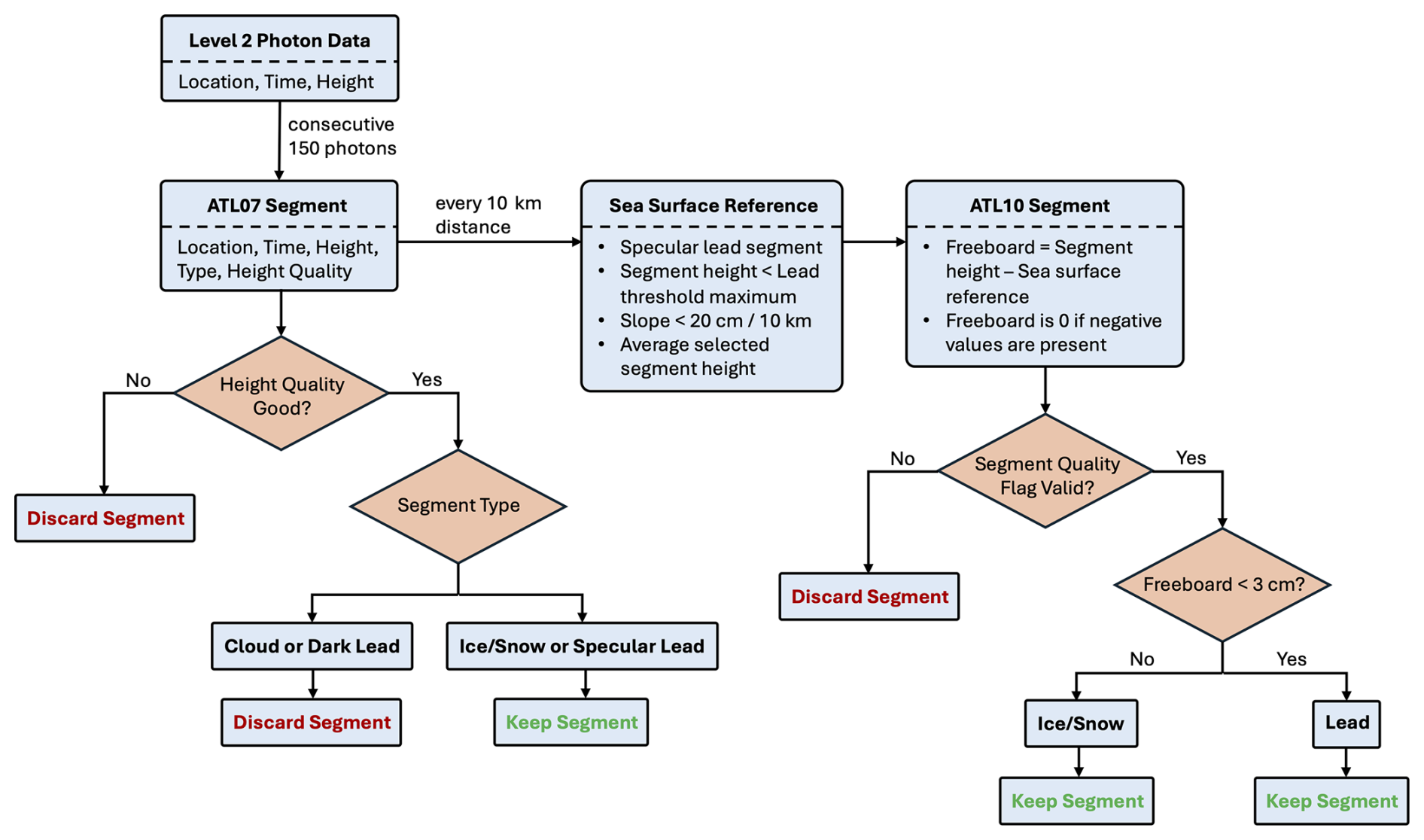
Figure 1 Major data processing steps in ATL07 and ATL10 to derive useful segments used in this study.

2.1 ATL07

ATL07 provides along-track sea ice height, including surface types and the height profiles of sea ice and open water leads, where ice concentration > 15 % (Kwok et al., 2022). In ATL07, 150 consecutive photons along a beam are aggregated to form a segment. The location/time of each segment is denoted as the average location/time of all photons within that segment. Based on the height histogram of these photons (fit into Gaussian), as well as surface and background photon rates and lidar parameters, the height and type of a segment are determined. Segment surface types are classified into clouds, ice/snow, and specular/dark leads. We only analyze segments that are marked as “good” in height segment quality, which was determined by the fitting of the observed histogram to a Gaussian distribution. Given that segments with bad height quality are often associated with rough/ridged surfaces, whereas lead detection is done on smooth surfaces, we don't expect the quality fit flags to cause issues with the lead detection. Generally, low surface rates (caused by low reflectance) indicate water/thin ice in leads, whereas high surface rates imply ice/snow. However, very high surface rates have also been observed from smooth open-water/thin ice surfaces. Therefore, leads are further classified into specular (with very high surface rates) and dark (with low surface rates) leads. Some specular leads are selected and marked to be sea surface height candidates that are used to derive sea surface reference in ATL10 (detailed in the next subsection). As dark leads are sometimes misclassified as clouds, they are not used as sea surface references in ATL10, and we will only show results of specular leads from ATL07.

As each segment consists of 150 photons, segment lengths vary across different surface types with various reflectance (Fig. 2a). Segment lengths are generally inversely related to surface photon rates: specular lead segments are shortest with very high surface rates, followed by ice/snow segments. Given that surface type is designated for each segment, segment lengths indicate the resolution of ATL07 in different surface types. ATL07 strong beams can resolve ice/snow surface in a resolution of ∼ 12 to 14 m (±5.5 m, half of the footprint size), and specular leads down to only ∼ 7.5 m (±5.5 m, Fig. 2a). We note that the detection of specular leads in ATL07 is very strict to avoid possible other surface types (mostly ice) to be classified as specular leads. Therefore, specular leads detected in ATL07 are likely a conservative estimate of total lead extent.

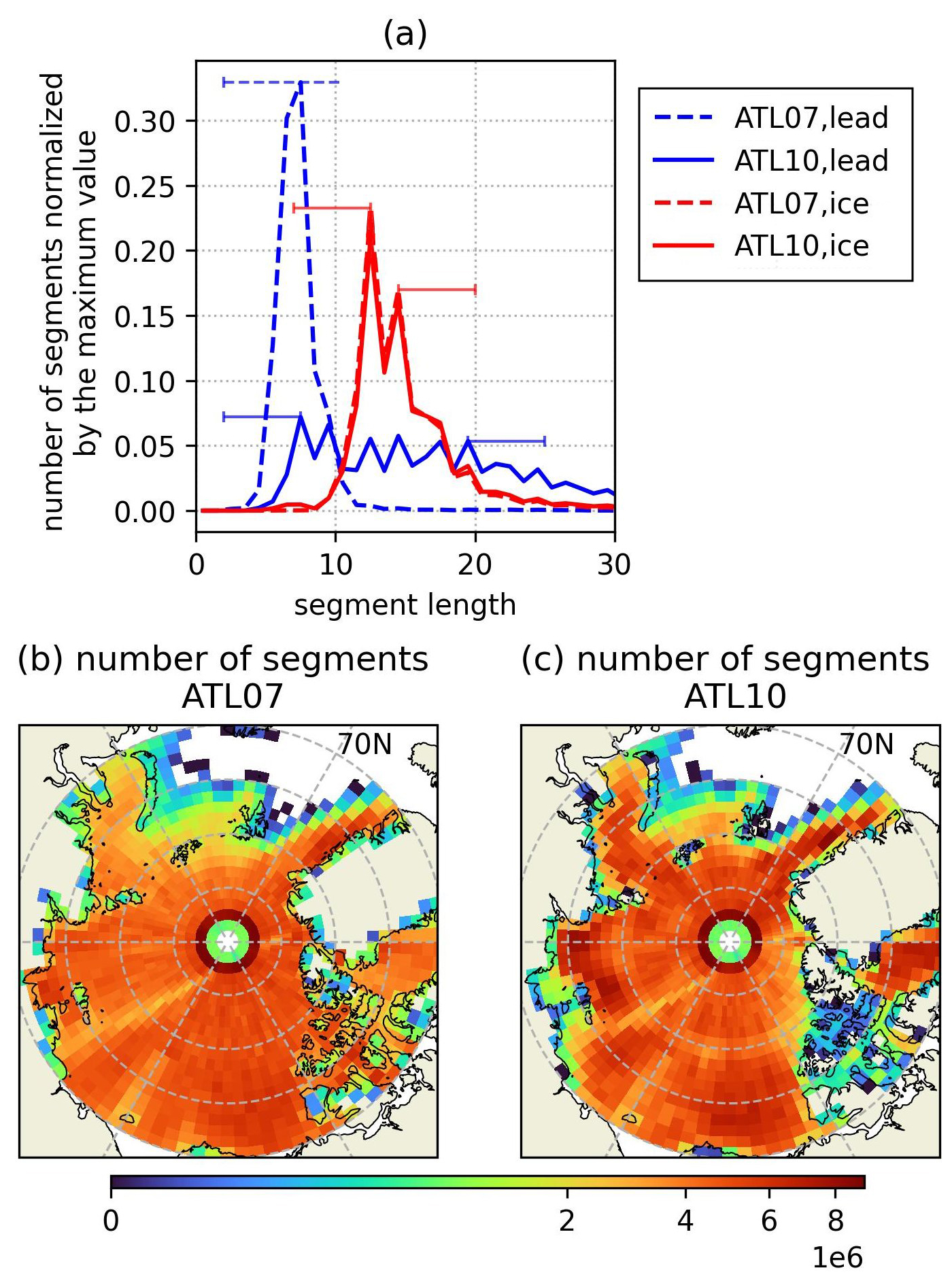
Figure 2 (a) Histogram of length of a single lead (blue) and ice (red) segment in ATL07 (dashed) and ATL10 (solid). Error bars represent half of the ICESat-2 footprint size (5.5 m). (b–c) Total number of segments in grid cells of 1° longitude × 4° latitude in the winter of 2018–2024 in (b) ATL07 and (c) ATL10.

Total segment number in ATL07 in November–April of 2018–2024 is on the order of 6×10⁶ (Fig. 2b), besides regions near coasts and ice edge, where total segment number reduces to ∼ 10⁶. The dense samplings of ICESat-2 indicate the statistical robustness of lead characterization.

Petty et al. (2021) (P21) assessed ICESat-2 ATL07 surface types product, and validated the along-track lead fraction in the first winter of the mission (2018–2019) with Sentinel-2 images. Several new releases of ICESat-2 ATL07 product have been published since P21, with longer records and improved algorithms, allowing improved characterization of lead statistics, such as sizes in addition to the areal fraction.

2.2 ATL10

ATL10 provides freeboard estimates using the same segments as ATL07, including those identified as leads, over regions with ice coverage > 50 %. For each 10 km distance along all beams, a single value of sea surface reference is first derived from all sea surface height candidates marked in ATL07. A specular lead segment is selected to be a sea surface reference candidate when its segment height is smaller than the lead threshold maximum height calculated from all segments over the 10 km distance. The lead threshold maximum height is the maximum of the two quantities: 2 % of valid heights within the 10 km track and the minimum value of a subset of valid heights where the segment is not on the edge of a data gap and the fitted Gaussian width is less than 0.13 m (see ATBD; Kwok et al., 2022). Freeboard is then calculated as the difference between the segment height and the sea surface reference. In cases where no sea surface height candidates are available in the 10 km distance, or the tilts in these candidates are larger than 20 cm per 10 km, the reference sea surface will be interpolated between two valid sea surface references if the time gap and height difference between the two sea surface references are small (see ATBD; Kwok et al., 2022). There will be cases where the estimated freeboard is negative because the derived sea surface reference is not local to each individual segment or a result of subsurface scattering in snow-free thin ice (Studinger et al., 2024); these negative values are truncated to zero in ATL10. A case study suggests that only ∼ 0.2 % of all segments are truncated to zero. Quality flags that describe the quality of the along-track Gaussian fit are also provided. We only use segments marked as valid in the quality flag.

In ATL10, we define a segment as lead segment when its freeboard is smaller than 3 cm. These lead segments include both open-water leads, as well as newly-closed ones, which represents a maximum ice and snow thickness in the lead of ∼ 30 cm. The choice of 3 cm is arbitrary to some degree, based on the representative uncertainty of ∼ 1–2 cm in ATL10 freeboard (Magruder et al., 2025). We will discuss the sensitivity of lead properties to the freeboard criterion in Sect. 5. ATL10 strong beams can resolve lead segment lengths to as small as 7.5 m (±5.5 m), same as ATL07 (Fig. 2a). The lengths of the lead segments in ATL10 range from 7.5 to ∼ 19.5 m (±5.5 m), as newly-freezing ice (moderate reflectance) and dark leads (low reflectance) are also identified as leads in ATL10. Total number of segments in ATL10 is comparable with those in ATL07 as expected, since ATL10 segments are based on the same segments in ATL07, with differences arising from ice concentration filters and quality flags.

3 Methods

We aggregate lead statistics over predefined geographic regions, and on a regular grid of 1° longitude × 4° latitude. We use a lat/long grid, instead of the commonly used 25 km × 25 km polar steographic projection in other high-level ICESat-2 products, to account for denser sampling at higher latitudes. On a 1° × 4° grid, the number of segments available in each grid cell is of similar magnitude (∼ 5 × 10⁶) south of 85°N. Even near the ICESat-2 orbit boundary of 88°N, the number of segments is still on the same order of magnitude as the ice-covered regions in lower latitudes (Fig. 2b–c).

3.1 Lead size

For each product, we first combine consecutive lead (ice) segments to form a single lead (ice floe). The size of a lead is then calculated as the distance between the first and last segment centers, plus half of the first and last segment length, given that the location of a segment is assigned to be the middle position of the segment. As introduced earlier, the footprint size (11 m) characterizes the uncertainty in lead (ice floe) sizes. We use “size” (equivalent to the term “apparent lead width” used in Wernecke and Kaleschke (2015)) instead of the commonly used “width”, as ICESat-2 tracks are not always perpendicular to leads to measure the actual “width”. Such orientation problems will be discussed later in the paper.

3.2 Lead fraction

Within a given grid cell (or region), lead fraction (L_f) is calculated as the total length of all leads divided by the length of all leads and ice floes defined in the previous section:

$$\begin{array}{}\text{(1)}& L_{\mathrm{f}}={\displaystyle \frac{{\sum }_{i=\mathrm{1}}^n{L}_i}{{\sum }_{i=\mathrm{1}}^n{L}_i+{\sum }_{j=\mathrm{1}}^N{L}_j}},\end{array}$$

in which L_i is the size of a given lead, n is the total number of leads, L_j is the size of a given ice floe, and N the total number of ice floes.

A lead/ice segment that crosses two grid cells (or regions) is assigned to the cell (region) encompassing its center. Given the meter to tens-of-meter scale of a single segment, we assume that the impact of such region-crossing segments is small.

We characterize uncertainties in lead fraction by two quantities: (1) their formal standard errors, and (2) lead fraction after accounting for footprint size. In (1), the formal standard errors in lead fraction are given by the ratio of their standard deviations to the square root of sampling size:

$$\begin{array}{}\text{(2)}& {\mathit{\sigma }}_{\mathrm{f}}=\sqrt{{\displaystyle \frac{{\sum }_{i=\mathrm{1}}^{N_{\mathrm{b}}}(L_{\mathrm{fb}}{}_i-\stackrel{\mathrm{‾}}{L_{\mathrm{fb}}}{)}^{\mathrm{2}}}{N_{\mathrm{b}}}}}/\sqrt{N_{\mathrm{b}}},\end{array}$$

where L_fbi is the lead fraction in an individual beam, $\stackrel{\mathrm{‾}}{L_{\mathrm{fb}}}$ is the averaged lead fraction over all beams within a given cell (region), and N_b represents the total number of beams. In (2), we calculate the lead fraction by adding (subtracting) the footprint size to (from) each individual lead and subtracting (adding) the footprint size from (to) each individual ice floe in equation (1) as:

$$\begin{array}{}\text{(3)}& {\displaystyle }{L}_{\mathrm{f}}^{\mathrm{low}}={\displaystyle \frac{{\sum }_{i=\mathrm{1}}^n(L_i-\mathrm{11})}{{\sum }_{i=\mathrm{1}}^n(L_i-\mathrm{11})+{\sum }_{j=\mathrm{1}}^N(L_j+\mathrm{11})}},\text{(4)}& {\displaystyle }{L}_{\mathrm{f}}^{\mathrm{high}}={\displaystyle \frac{{\sum }_{i=\mathrm{1}}^n(L_i+\mathrm{11})}{{\sum }_{i=\mathrm{1}}^n(L_i+\mathrm{11})+{\sum }_{j=\mathrm{1}}^N(L_j-\mathrm{11})}},\end{array}$$

in which $L_{\mathrm{f}}^{\mathrm{low}}$ and $L_{\mathrm{f}}^{\mathrm{high}}$ are the lower and upper estimates of the lead fraction.

The two quantities described above quantify different aspects of uncertainties. Standard errors suggest the representativeness of the cell-mean lead fraction calculated by equation (1). The lower and upper estimates of the lead fraction indicate the uncertainties associated with the geolocation of photons.

4 Results

4.1 Climatology

4.1.1 Lead fraction

Climatological wintertime lead fraction $L_{\mathrm{f}}^{\mathrm{clim}}$, calculated using all segments across the Arctic in each grid cell following equation (1), shows a robust spatial pattern in both products: the largest lead fraction is found near the ice edge, with decreases towards the Central Arctic (Fig. 3a, b). In total, the lead fraction in ATL10 is ∼ 5 times larger than that in ATL07, given that only a subset of leads (i.e., specular leads) are accounted for in ATL07. The ratio of $L_{\mathrm{f}}^{\mathrm{clim}}$ between the two products is not consistent throughout the Arctic: the smallest ratio is present near ice edge, and becomes larger towards the Central Arctic, opposite to lead fraction spatial pattern. We will discuss the potential reasons in the discussion section.

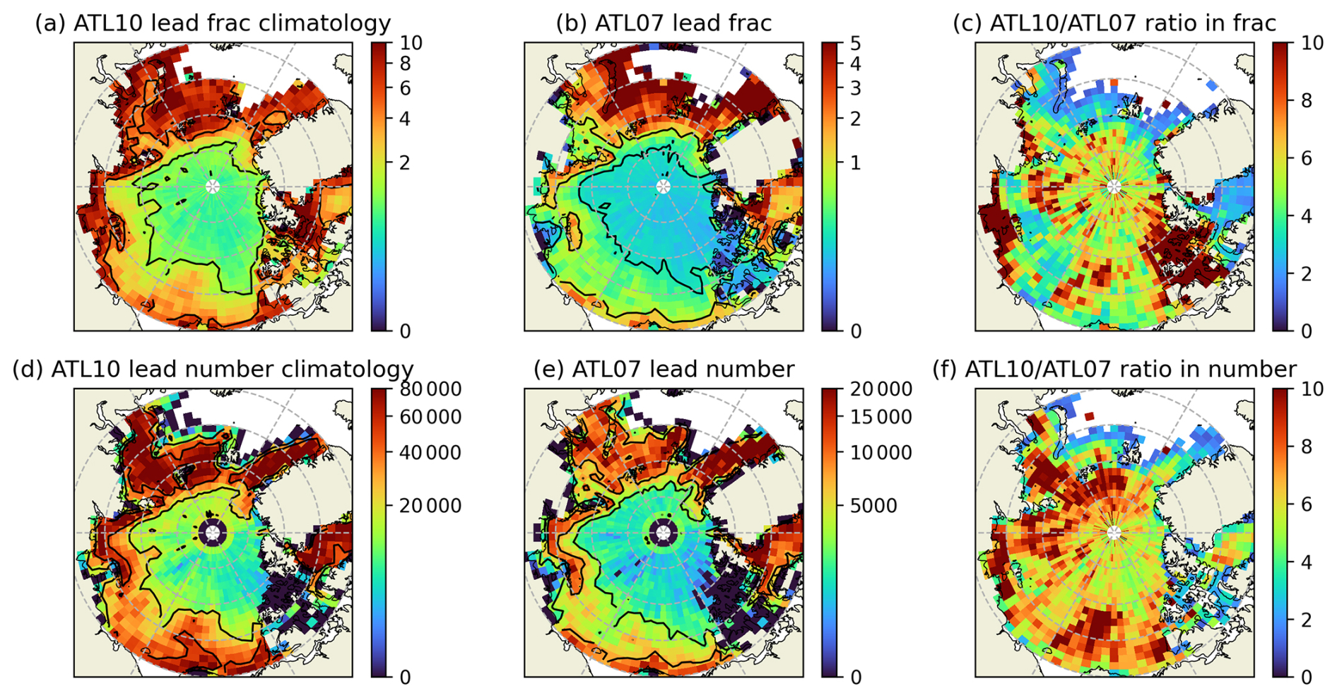
Figure 3 (a, b, d, e) Climatological wintertime (a, b) lead fraction and (d, e) lead number in (a, d) ATL10 and (b, e) ATL07. Contours in (a) and (b) indicate 1.3 % and 5 %, and 0.2 % and 1 %. Contours in (d) and (e) indicate 20 000 and 50 000, and 3000 and 7500. (c, f) The ratio of (c) lead fraction and (f) number in ATL10 to those in ATL07.

In ATL10 (ATL07), in the abyssal plain, $L_{\mathrm{f}}^{\mathrm{clim}}$ is < 1.3 % (0.2 %). More leads (> 2 % for ATL10 and > 0.5 % for ATL07) are present over the continental shelves. A stripe of high $L_{\mathrm{f}}^{\mathrm{clim}}$ (> 5 % for ATL10 and > 1 % for ATL07) from ∼ 90° E to ∼ 120° W is present, following the coastline. In Nordic Seas and Baffin Bay in the periphery of the ice cover, $L_{\mathrm{f}}^{\mathrm{clim}}$ can reach more than 10 %.

Despite the general consistency in $L_{\mathrm{f}}^{\mathrm{clim}}$ spatial distribution in both products, we find two regions of noticeable disagreement: the Canadian Arctic Archipelago and south of the New Siberian Islands. These two regions are also revealed by the anomalously large ATL10-ATL07 $L_{\mathrm{f}}^{\mathrm{clim}}$ ratio (Fig. 3c).

The total number of leads in the winter of 2018–2024 follows a similar spatial pattern as $L_{\mathrm{f}}^{\mathrm{clim}}$ (Fig. 3d, e). In the Canadian Arctic Archipelago where $L_{\mathrm{f}}^{\mathrm{clim}}$ in ATL10 is more than 10 times larger than that in ATL07, lead numbers in both products are comparable, suggesting larger average lead size in ATL10. Similar conclusions can be drawn for the south of the New Siberian Islands, where the ratio of $L_{\mathrm{f}}^{\mathrm{clim}}$ in ATL10 to ATL07 is much bigger than that of lead number. On the contrary, in the remainder of the Arctic (excluding the region of multi-year sea ice, i.e., north of Greenland and the Canadian Arctic Archipelago), the ratio of $L_{\mathrm{f}}^{\mathrm{clim}}$ between the two products is smaller than the ratio of lead number, suggesting a smaller average lead size in ATL10.

The larger average lead size in ATL10 compared to ATL07 in the Canadian Arctic Archipelago and the New Siberian Islands indicates the predominance of non-specular leads in these regions, as larger leads allow for the development of rougher sea surfaces with low specularity. This is consistent with the considerably higher lead fractions found in ATL10 than in ATL07 (Fig. 3a, b).

4.1.2 Lead size

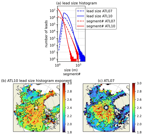
We next examine the pan-Arctic lead size distribution over the entire winter periods for both products (Fig. 4a, blue lines). The lead size histogram peaks at 7.5 m (±5.5 m, ATL10) and 10.5 m (±5.5 m, ATL07). This peak is likely associated with the resolution (i.e., segment length) limitation, rather than the actual lead size distribution. Indeed, the majority of leads consist of one segment (Fig. 4a, red lines), suggesting that lead size histogram is truncated at ICESat-2's effective resolution.

Figure 4 (a) Histogram of individual lead size (blue) and the number of segments that consist of a single lead (red), from ATL07 (dashed) and ATL10 (solid). (b–c) Exponents of the power-law distribution of lead size estimated between lead size of 20 and 100 m in (b) ATL10 and (c) ATL07. Only cells with p-value < 0.05 when estimating histogram slopes are shown.

On the right side of the peak, the histogram follows a power-law distribution; the exponent of lead size estimated between 20 and 100 m in ATL07 yields 2.1 ± 0.01, and in ATL10 2.4 ± 0.04, comparable to previous studies (Marcq and Weiss, 2012; Wernecke and Kaleschke, 2015). The magnitude of the exponent increases with lead sizes, reaching 3.5 ± 0.02 (ATL10) and 2.5 ± 0.01 (ATL07) between 100 and 1000 m. The steepening slope of the lead size histogram on logarithmic scale (i.e., increasing exponent) with lead size could be an artifact of the discrete lead sizes (the sum of individual segment length), which has a greater effect at smaller lead sizes where a single lead comprises only a few segments. However, because a similar steepening slope is also present in the segment number histogram (Fig. 4a, red lines), the steepening slope of the lead size histogram is more likely a real property of leads. Indeed, very large leads (> a few hundred meters) are rare: only ∼ 30 leads of size ∼ 1000 m are present in the 6-year winter ICESat-2 record.

To examine spatial variations in lead size, we estimate the log-log slope between 20 and 100 m in each grid cell. (Grid-cell mean values are not representative of spatial differences, given the power-law distribution of leads). The spatial distribution of the histogram slope (Fig. 4b, c), despite appearing noisy, is consistent with that of the lead fraction in Fig. 3a, b. The largest slopes are found in the Central Arctic, up to ∼ 3 in both products, indicating the presence of more small leads than big ones, compared to regions of the Barents Sea/Baffin Bay and the coasts (with slopes of ∼ 2.4 in ATL10 and ∼ 1.9 in ATL07), where slopes are generally smaller. In most of the Arctic, power-law slopes in ATL10 are greater than that in ATL07, except for a few cells in the Central Arctic, suggesting the larger percentage of small leads (between 20 and 100 m) in ATL10, consistent with the smaller average lead size in ATL10 suggested by Fig. 3c, f.

4.2 Interannual Variations

4.2.1 Lead fraction

We next identify significant year-to-year variations in lead fraction from both products. In Fig. 5, we show the lead fraction anomaly relative to climatology in each grid cell. To highlight common features, only grid cells with the same sign in both products are shown (∼ 60 % to ∼ 70 % of grid cells). Four prominent features are evident: (1) a maximum in the Central Arctic in the winter of 2020–2021; (2) a minimum in the Chukchi/Beaufort Sea in 2021–2022; (3) a decreasing trend over the Laptev Sea; (4) an increasing trend in the multi-year sea ice region (i.e., north of Greenland and the Canadian Arctic Archipelago).

Figure 5 Lead fraction anomaly relative to their climatology (%) in each winter from (top row) ATL10 and (bottom row) ATL07. Only grid cells with the same signs in lead fraction anomaly derived from the two products are shown, highlighting features that are consistent between the two products.

To further examine lead fraction variations in these four regions, we aggregate all data in a given region (in contrast to grid cell basis) (Fig. 6). All regions exhibit statistically significant variability over the 6-winter record, with small standard errors. Lead fraction uncertainties associated with footprint size calculated following Sect. 3.2 amount to ∼ 30 % of the mean value. Although the magnitude of interannual variations in lead fraction varies across products, their regional interannual evolution are robust, and are consistent with the four features evident in Fig. 5.

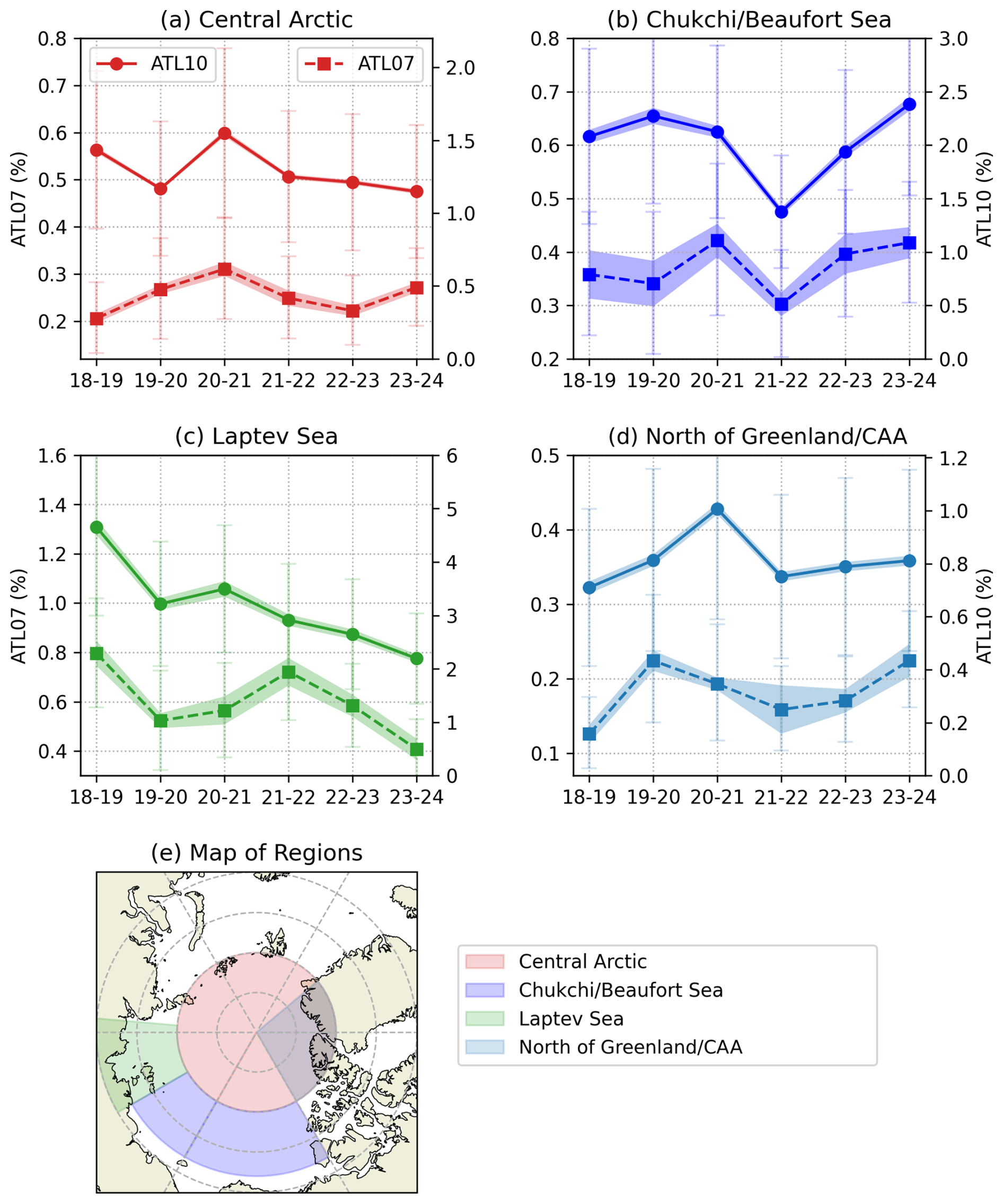
Figure 6 Yearly mean lead fraction in (a) Central Arctic, (b) Chukchi/Beaufort Sea, (c) Laptev Sea, and (d) north of Greenland and the Canadian Arctic Archipelago (CAA), calculated using all data in a given region defined in (e) from ATL10 (dots and solid lines) and ATL07 (squares and dashed lines). Values in ATL07 are shown on the left y-axis, and ATL10 on the right y-axis. Shading indicates the standard error associated with the mean value. Error bars denote lead fraction uncertainties associated with footprint size.

4.2.2 Changes in leads by size class

We next examine whether prominent variations in the lead fraction (introduced above) are disproportionately due to changes in specific lead size classes. For each lead size class in both ATL07 and ATL10, we calculate the ratio of lead number in 2020–2021 for the Central Arctic and in 2021–2022 for Chukchi/Beaufort Sea (when lead fraction is maximum or minimum, respectively) to the lead number in the previous year, and the ratio of lead number in 2023–2024 to that in 2018–2019 in the other two regions where lead fraction shows a trend (Fig. 7).

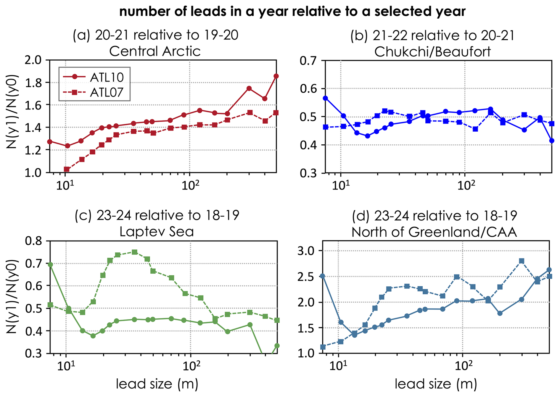
Figure 7 Ratio of lead number in the year with signature lead fraction to lead number in a selected year ($N\left(y\mathrm{1}\right)/N\left(y\mathrm{0}\right)$, y-axis) in varying lead sizes (x-axis). Solid curves with dots represent ATL10 and dashed curves with squares represent ATL07. (a) Central Arctic in 2020–2021 to 2019–2020. (b) Chukchi/Beaufort Sea in 2021–2022 to 2020–2021. (c) Laptev Sea in 2023–2024 to 2018–2019. (d) North of Greenland and the Canadian Arctic Archipelago (CAA) in 2023–2024 to 2018–2019.

Changes in lead number over varying sizes show some consistency between ATL07 and ATL10. In the Central Arctic (Fig. 7a), in the winter of 2020–2021, the lead number ratio is larger than 1, i.e., an increase in the number of leads of all sizes compared to the preceding season. In addition, the increases in bigger leads ($>\sim$100 m) are greater than smaller ones. A similar pattern is found in the north of Greenland and the Canadian Arctic Archipelago (Fig. 7d), where lead fraction shows an increasing trend over the past 6 winters.

Over the Chukchi/Beaufort Sea (Fig. 7b), the lead number ratio is smaller than 1, but of comparable magnitude for all lead sizes, suggesting that the decrease in lead fraction in 2021–2022 relative to the previous year is attributable to leads of all sizes.

In the Laptev Sea, where lead fraction shows a decreasing trend, decreases are evident across all size classes in both products. The ratio is higher for leads of ∼ 20 to ∼ 90 m in ATL07, indicating that decreases in leads in this range play a lesser role in the lead fraction decrease. Such behavior is less evident in ATL10.

A notable feature in Fig. 7 for ATL10 is the dip at lead size ∼ 10–15 m in all four regions, that is not present for ATL07. Leads in this range exhibit a small increase (a large drop) when lead fraction increases (decreases) compared to leads of a few meters. The discrepancy between ATL07 and ATL10 in this size range could be associated with the inclusion of non-specular leads in ATL10, whose sizes fall within this range (see Fig. 4a).

5 Conclusions and Discussions

In this work, we characterize the Arctic Ocean's wintertime sea ice leads from the high-resolution ICESat-2 ATL07 and ATL10 products over the period of October 2018 to April 2024. On the climatological scale, lead fraction has a robust spatial pattern in both products, highest near the Barents Sea and along the coasts (> 10 %), with substantially smaller values in the Central Arctic (< 1 %). Lead size generally follows a power-law distribution, with exponents between 2 and 3 and a notable decrease in the exponent at smaller lead size. Power-law exponents exhibit an increase from lower latitudes towards the high-latitude Central Arctic.

We found four notable interannual variations in lead fraction, including: a maximum in 2020–2021 in the Central Arctic, a minimum in the Chukchi/Beaufort Sea in 2020–2021, a decreasing trend in the Laptev Sea, and an increasing trend in the north of Greenland and the Canadian Arctic Archipelago. Leads of varying sizes play different roles in the lead fraction interannual variations: in general, bigger leads exhibit a greater increase when lead fraction increases, whereas leads of all sizes decrease at a similar rate when lead fraction decreases. If the relationship between the lead size distribution and lead fraction holds for other regions and time periods, it implies that Arctic sea ice is evolving towards a state with more large leads over the past 6 years.

Although we do not examine the drivers of interannual variations here, it is likely that there is some role for sea ice thickness anomalies, which precondition ice deformation and lead formation. Consistent with this inference, February and March averaged sea ice thickness derived from CryoSat-2 and ICESat-2 are found to be minimum in the Central Arctic in 2021, and maximum in the Chukchi/Beaufort Sea in 2022 compared to adjacent years. Sea ice exhibits a thinning trend in the multiyear-ice region, and a weak thickening trend in the Laptev Sea (Kacimi and Kwok, 2024). We note that cyclone activities could also favor lead formation. For example, anomalously high cyclone counts and durations are reported in the winter of 2020–2021 (Zhang et al., 2023), which could explain the lead fraction maximum in the Central Arctic in the same winter. Ocean processes, sea ice internal stress and inertial forces may play important roles as well.

In addition to results shared by ATL07 and ATL10, some inter-product discrepancies are evident. A detailed analysis of discrepancies is not feasible in the pan-Arctic. However, a previously published case study provides some evidence comparing ATL07/10 products with Sentinel-2 imagery (Petty et al., 2021), which shows that ATL10 is capable of capturing leads that are closed for a longer time, beyond the open or freshly closed ones detected by ATL07. Over most of the Arctic, the magnitude of the lead fraction is ∼ 5 times greater in ATL10 than in ATL07. This ratio is not uniform across the Arctic: it is anomalously large (> 10) in the Canadian Arctic Archipelago and south of New Siberian Islands, and smaller near the Barents Sea/Baffin Bay (< 3). Over most of the Arctic, the lead size power-law exponent is larger in ATL10 than that in ATL07, consistent with the inclusion of non-specular leads in ATL10.

5.1 Climatological lead properties

The spatial patterns of lead fraction, number, and power-law exponents are generally consistent with ice thickness: ice edges are more prone to breaking due to wind stress or ocean circulation, leading to larger leads. Specifically, a band of high lead fraction (> 1 % in ATL07 and > 5 % in ATL10) from ∼ 90° E to ∼ 120° W is present following the coastline. This stripe appears to co-locate with coastal shelf waves (Danielson et al., 2020), likely driven by the cross-shelf Ekman transport from local winds (Fukumori et al., 2015). These constantly generated waves could result in more ice breaking, preconditioned by the thinner ice near the coast, likely yielding the observed high lead fraction. The ratio of the lead fraction in ATL10 to that in ATL07 is smaller in the Barents Sea and Baffin Bay area compared to the Central Arctic. An explanation could be that open leads are quickly refrozen in the Central Arctic compared to ice edges, resulting in more newly closed leads that are considered as leads in ATL10 but not in ATL07.

The power-law distribution of the sea ice leads reflects the fractal nature and nonlinearity in sea ice fracturing, which exhibit self-similar behavior that is often generated by repeated physical growth process (Vicsek, 1992). Many other variables exhibit the same fractal nature that follows a power-law distribution of their sizes, including the complementary solid component of the ice cover – sea ice floes (e.g., Toyota et al., 2006; Stern et al., 2018a, b; Christensen and Driver, 2021). Here, we find evidence that the power-law exponent increases with lead size and varies across regions and time, likely reflecting differences in winds (e.g., Wang et al., 2016a, b) and ocean forcing like waves (e.g., Wang et al., 2016b; Voermans et al., 2020) acting on varying sea ice conditions that modulate its resistance to deformation (Herman, 2017; Heorton et al., 2018). Lead refreezing rate under different thermodynamic and dynamic processes may also contribute to the scale-dependent power-law exponent.

An increasing power-law exponent has been theorized (Rothrock and Thorndike, 1984) and observed (Toyota et al., 2006) for sea ice floes. Regional and temporal variability in floe size exponents has likewise been linked to the growth–melt cycle and ice precondition (e.g., Steer et al., 2008; Toyota et al., 2011; Stern et al., 2018a, b). Collectively, our results, and those for sea ice floes, suggests that assumptions of a (constant) power-law distribution could potentially give rise to the misrepresentation of sea ice simulations (see Horvat and Tziperman, 2017). In the future, taking into consideration the size-, region-, and time-varying exponent could be useful for the parameterization of lead effects in models.

As noted previously, ICESat-2 measurements are not sufficient to determine the orientation of leads; however, previous studies using MODIS and AMSR-E found that leads greater than 1 km are anisotropic: more leads are found to align closer to the north-south direction (< 60° or > 120° east of north) than the west–east direction, although regional variations are present (e.g., Br\öhan and Kaleschke, 2014; Hoffman et al., 2019).

The pan-Arctic spatial distribution of the climatological lead fraction in our study is qualitatively consistent with that from other satellites like MODIS (Willmes et al., 2015; Reiser et al., 2020; Willmes et al., 2023), Envisat and CryoSat-2 (Tilling et al., 2019). However, a quantitative comparison is challenging, given the different time periods in these studies and the different definitions in the lead fraction. For example, lead frequency, the ratio of lead counts over the total number of counts per pixel and month/year, is used to characterize sea ice occurrence in MODIS (Willmes et al., 2015, 2023), while the percentage of lead waveforms are used in Envisat and CryoSat-2 work (Tilling et al., 2019). We note that lead fraction reported here from ATL07 is likely substantially lower than those derived from the satellites mentioned above (e.g., Tilling et al., 2026), because ATL07 lead detection algorithm identifies only reliable specular leads.

5.2 Uncertainties in lead detection from ATL10

As outlined in Sect. 2.2, we classify segments with freeboard height smaller than 3 cm as leads. Raising this threshold would result in the inclusion of more thin ice as recently closed leads, and vice versa. The impact of a large threshold is especially pronounced in regions of newly formed sea ice, where thin ice may be erroneously classified as leads.

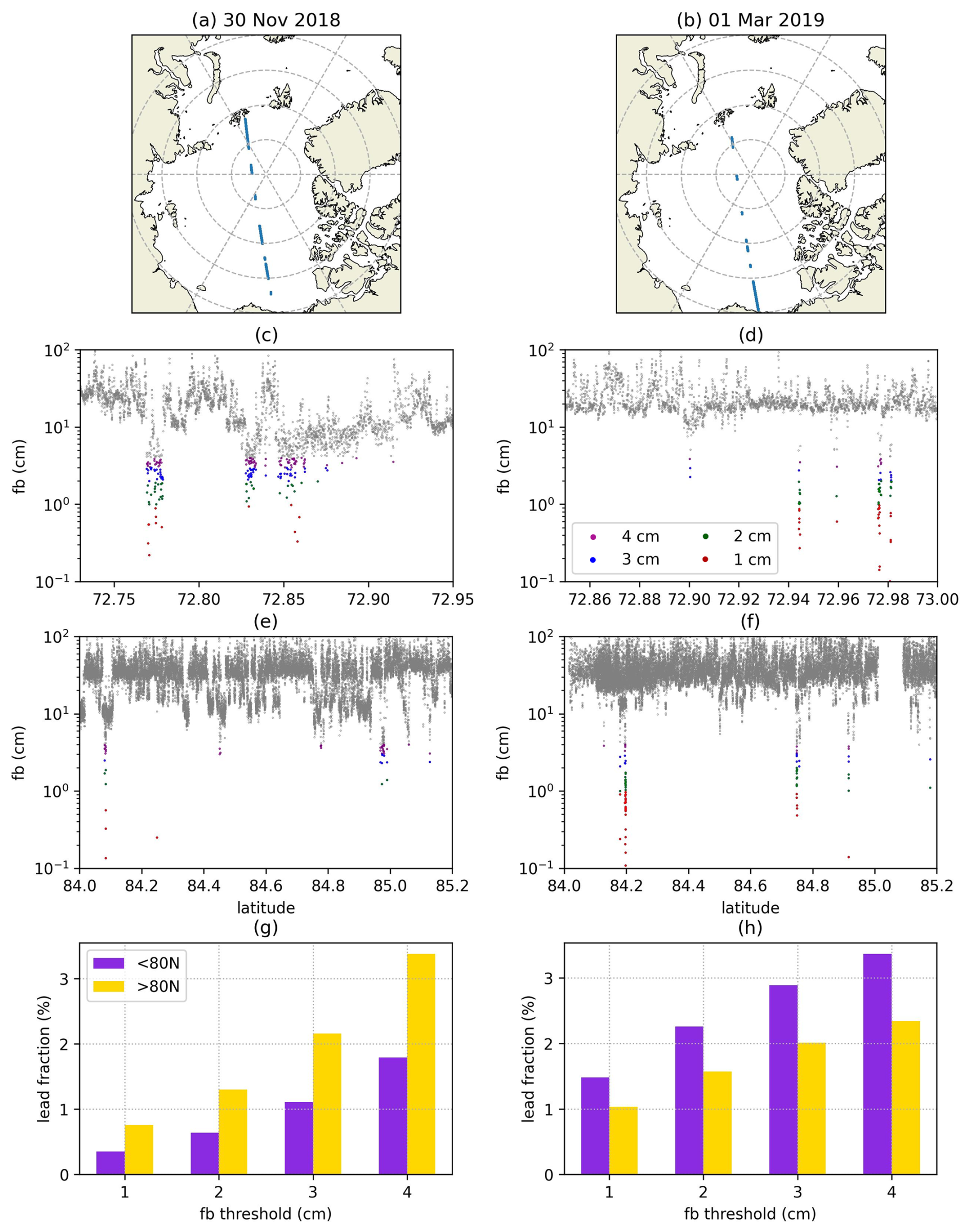
Figure 8 (a, b) Selected ICESat-2 track on (a) 30 November 2018 and (b) 1 March 2019. Only segments with freeboard less than 5 m and the quality check passed are shown. The total numbers of segments are 178594 on 30 November 2018 and 131663 on 1 March 2019. (c, f) Snapshots of freeboard over the part of the track with (c, d) thinner and thicker (e, f) ice in (c, e) November and (d, f) March. (g, h) Along-track lead fraction in regions of (g) thinner (south of 80°) and (h) thicker (north of 80°) ice.

To assess the influence of the freeboard height criterion on ATL10-derived lead detection, we select two ATL10 tracks across the Arctic in different time periods, one on 30 November 2018 during the growth season, and the other on when ice is near its seasonal maximum (1 March 2019; Fig. 8a, b). We then identify leads based on varying freeboard thresholds from 1 to 4 cm. The two freeboard snapshots on part of the tracks over thinner ice (Fig. 8c, d) and thicker ice (Fig. 8e, f) reveal a larger difference in lead detection in November over thinner ice with varying threshold values, compared to that in March and to regions with thicker ice during November. Indeed, the along-track lead fraction over thinner (< 80° N) and thicker (> 80° N) ice (Fig. 8g, h) exhibits the greatest relative increase in November south of 80°N, by 511 % when using a freeboard threshold of 4 cm instead of 1 cm. Despite the difference in the magnitude of lead fraction using varying thresholds, excluding November from our calculations does not qualitatively change the climatological and interannual variations in lead fraction (not shown). In fact, no perfect threshold can be selected, as ice grows quickly in new leads during winter. Therefore, instead of pursuing a perfect threshold, we use 3 cm, equivalent to the ice and snow thickness of ∼ 30 cm, regardless of seasons and sea ice states, to distinguish leads from pack ice and characterize the near pan-Arctic winter ice leads.

Another source of uncertainty in ATL10 lead detection arises from the reference sea surface used to derive freeboard height. As described in Sect. 2.2, the reference sea surface is not locally defined but instead represents the average sea surface height along a 10 km segment. In addition, if no reference surface can be determined due to lack of data, it is obtained through interpolation of adjacent surfaces. The uncertainties associated with the reference sea surface propagate to the freeboard estimates and, consequently, affect the lead detection.

5.3 Future potential improvements

Although our work used officially released ICESat-2 products to characterize the pan-Arctic lead fields in the ICESat-2 era, lead properties are dependent on the processing method, for example, the removal of dark leads in ATL07 and the freeboard threshold used in ATL10. Our study suggests that, despite the limitation in perfectly identifying the “true” leads, ICESat-2 is capable of representing lead characteristics in climatological and annual scales.

Ongoing efforts continue to improve the algorithm to detect leads from ICESat-2 measurements. These advances include, but not limited to, machine learning approaches developed by Koo et al. (2023) and Liu et al. (2025), and improved photon aggregation and height filtering criteria introduced by Farrell et al. (2020). These new techniques were validated using coincident Sentinel-2 imagery, and are thus limited to specific times and locations. Extending the application of these new methodologies to the full record of ICESat-2 measurements over the entire Arctic could potentially reduce the uncertainties in lead statistics.

Our analyses focus on the winter season to minimize the effects from other open-water features such as melt ponds and polynyas. A new two-month ICESat-2-derived melt pond characteristics in the melting season has been published based on the density-dimension algorithm (Herzfeld et al., 2024). A better quantification of the role of leads in the Arctic climate system over the melting season could be possible when a longer record of melt pond data becomes available.