The Modèle Atmosphérique Régional – Intelligence Artificielle (MAR-IA): surface meltwater over Greenland

Surface melting over the Greenland Ice Sheet has become one of the dominant sources of contemporary and projected global sea-level rise, with melt rates accelerating over recent decades. Understanding those processes and feedbacks that control Greenland's surface melt is central to improving projections of future mass loss and to clarifying how changes in surface energy balance components shape ice-sheet stability.

To this aim, we developed MAR-IA - a machine-learning emulator of the MAR regional climate model – designed to emulate daily surface meltwater production over Greenland and to enable attribution of melt drivers. We implement two complementary emulators: a high-fidelity MAR-IA trained on full MAR surface energy balance fields and a reanalysis-compatible MAR-IA-ERA trained on predictors available from products such as ERA5, thereby extending applicability beyond MAR-specific outputs. Both emulators employ gradient-boosted trees optimized via Bayesian hyperparameter search, achieving high test-set skill, with the best-performing final configuration reaching R²=0.987, low root mean squared error (<10 mm w.e. d⁻¹), and negligible bias relative to MAR meltwater outputs. We apply an explainable artificial intelligence (AI) analysis based on Shapley Additive Explanations (SHAP) to quantify how the importance of surface energy balance components,e.g., albedo, shortwave and longwave radiation, etc.,evolves across space and time over Greenland. Our results reveal robust spatial and temporal patterns in the dominance of radiative versus non-radiative drivers and demonstrate long-term trends in the relative contribution of temperature, shortwave radiation, and albedo to melt variability. These findings show that emulators can be used as powerful tools to complement regional climate models by enabling computationally efficient ensemble simulations and physically interpretable attribution of past and future Greenland surface melt.

1 Introduction

Surface melting over the Greenland Ice Sheet (GrIS) has emerged as one of the dominant contributors to contemporary and projected sea-level rise, with melt rates accelerating markedly over recent decades (Box et al., 2012; van den Broeke et al., 2016; Fettweis et al., 2020; Tedesco et al., 2016; Zhang et al., 2025). In this regard, it is crucial to understand the physical processes and feedbacks driving increased melt for improving projections of future mass loss and for elucidating the interactions among components of the surface energy and mass balance (Noël et al., 2015; Tedesco et al., 2016; Hofer et al., 2017; Lenaerts et al., 2019).

Regional climate models (RCMs), including the Modèle Atmosphérique Régional (MAR, Fettweis et al., 2013), Regional Atmospheric Climate Model (RACMO Noël et al., 2018), and HIRHAM (a regional climate model based on the High Resolution Limited Area Model, HIRLAM, and ECHAM physics; Langen et al., 2017), have substantially advanced our ability to simulate surface melt and better capture the surface energy- and mass-balance processes that govern meltwater production. Nevertheless, disentangling the complex, non-linear relationships among surface energy balance (SEB) components, such as albedo, surface temperature, and shortwave and longwave radiation, and their influence on surface melt remains computationally demanding and formally ill-posed (Mioduszewski et al., 2014). This limits the feasibility of large-ensemble simulations and hinder the systematic attribution of melt variability to individual drivers.

Recent developments in machine learning (ML) and explainable artificial intelligence (XAI) offer promising pathways to address such limitations. ML-based emulators can replicate RCM outputs with high fidelity while substantially reducing computational costs, enabling ensemble simulations and supporting model-interpretation analyses (Reichstein et al., 2019; Doury et al., 2023). Tree-based algorithms such as eXtreme Gradient Boosting (XGBoost) (Chen and Guestrin, 2016), deep convolutional neural networks (LeCun et al., 2015), and ensemble approaches (Materia et al., 2024) have been increasingly applied in Earth system science. When trained on RCM outputs, such models have the potential to emulate melt-related behavior and support attribution analyses using interpretable frameworks such as SHapley Additive exPlanations (SHAP; Lundberg and Lee, 2017).

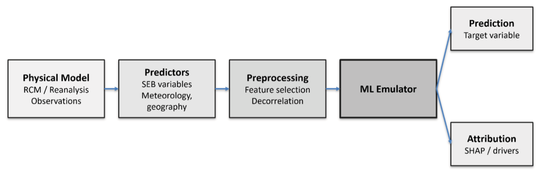
Recent cryosphere-focused studies illustrate several related but distinct uses of machine learning. Lütjens et al. (2025) developed a deep-learning framework for spatiotemporal downscaling of surface meltwater by combining remote sensing and physics-based model output over Helheim Glacier. Bochow et al. (2025) used a physics-constrained generative ML framework trained on MAR to downscale monthly Greenland surface mass balance and surface temperature fields to higher spatial resolution. A more closely related recent study is Schlager et al. (2026), who developed a neural-network emulator of daily Greenland surface melt trained on output from the polar regional climate model HIRHAM5 and its firn model. Related cryosphere emulation efforts also include the emulation of firn-hydrology-related processes in Antarctica, further illustrating the growing role of ML emulators in polar climate applications (Veldhuijsen et al., 2025). In contrast, our contribution lies in the direct emulation of daily surface meltwater production from MAR and in the interpretable attribution of the dominant melt drivers across Greenland in space and time. Here, we introduce a novel ML-based emulator, the Modèle Atmosphérique Régional – Intelligence Artificielle (MAR-IA), trained on daily meltwater production (mm w.e. d⁻¹) simulated by MAR for the period 1979–2024. The predictor set includes SEB components and near-surface meteorological variables. We implemented two complementary training strategies: (1) a high-fidelity emulator (MAR-IA) optimized to minimize errors relative to MAR outputs using full SEB predictors, and (2) a reanalysis-compatible emulator (MAR-IA-ERA) trained on predictors available from a widely used dataset, ERA5 (Hersbach et al., 2020), enhancing applicability beyond MAR-specific outputs. In the MAR-IA-ERA configuration, ERA5 variables are reprojected to the MAR grid but are not dynamically downscaled to MAR-consistent fields. We therefore view this setup as a practical reanalysis-compatible emulator input strategy rather than a substitute for dedicated downscaling and note that ongoing ML-based downscaling developments are highly relevant for improving such applications (Doury et al., 2023; Bochow et al., 2025; Lütjens et al., 2025). Following the development of the emulators, we apply SHAP-based model interpretation to quantify the emulator-attributed importance of SEB components, such as albedo and incoming shortwave and longwave radiation, over the historical period (1979–2024). This approach provides a way to assess whether the learned predictor–melt relationships are broadly consistent with known melt physics and demonstrates the potential for interpretable ML models in cryospheric research. Our findings highlight the potential of ML emulators to complement traditional modeling frameworks, enabling computationally efficient simulations and robust attribution of melt drivers under past and future climate conditions. A conceptual overview of the MAR-IA framework is shown in Fig. 1.

Figure 1 Conceptual overview of the MAR-IA framework.

2 Methods and data

2.1 The MAR model

We use the outputs from the Modèle Atmosphérique Régional (MAR), a regional climate model designed to simulate atmosphere–surface interactions over the Greenland ice sheet (Fettweis et al., 2017; Tedesco et al., 2023). The model was developed for simulations of polar and mountainous climates, with a particular focus on the surface mass balance (SMB) of ice sheets and glaciers (Fettweis, 2007; Franco et al., 2012) and has been extensively used to study the Greenland and Antarctic Ice Sheets (Agosta et al., 2019; Smith et al., 2023). MAR incorporates a three-dimensional atmospheric model coupled with a multilayer snow model, which allows it to resolve energy and mass exchanges at the snow–atmosphere interface, including processes such as meltwater percolation, refreezing, and densification (Brun et al., 1992).

The atmospheric component of MAR is forced at the boundaries of the Greenland region using data from global reanalysis products. For the MAR simulations used here, MAR was forced by the ERA5 product, produced by the European Centre for Medium-Range Weather Forecasts (ECMWF) (Hersbach et al., 2020). ERA5 is a global reanalysis dataset that combines observations from satellites, ground stations, and radiosondes with a numerical weather prediction model to provide hourly estimates of atmospheric, land, and ocean variables since 1940 (Delhasse et al., 2020). With a horizontal resolution of approximately 31 km, 137 vertical levels, and a detailed vertical structure, ERA5 offers comprehensive coverage of variables such as geopotential height, temperature, humidity, wind speed, and radiative and turbulent surface fluxes (Hersbach et al., 2020; Delhasse et al., 2020).

In the context of surface meltwater prediction, variables of primary interest include surface albedo (modeled through snow grain properties in Crocus), which controls reflected versus absorbed solar radiation (Brun et al., 1992; Tedesco et al., 2016; Coléou and Lesaffre, 1998); and 2 m air temperature, a critical driver of melt energy. Radiative components such as downward shortwave and longwave radiation influence the surface energy balance, while turbulent fluxes of sensible and latent heat reflect energy exchange through convection and moisture transport (Hersbach et al., 2020; Delhasse et al., 2020; Wang et al., 2021). Topographic variables,elevation, latitude, and longitude,also modulate the local energy balance and atmospheric conditions (Tedesco et al., 2016a, b; Fettweis et al., 2017). These predictors are used to train our model, as explained in Sect. 2.3.

2.2 The XGBoost algorithm

Machine learning algorithms have become increasingly popular for extracting insights from complex datasets and making predictions from data. Among these algorithms, the eXtreme Gradient Boosting (XGBoost) algorithm has become one of the most popular due to its performance, accuracy, ability to handle a variety of data types, and capacity for processing large datasets (Chen and Guestrin 2016, Bentéjac et al., 2021). In this study, XGBoost was selected because our emulator is trained on a large tabular regression dataset composed of surface energy balance, meteorological, and geographic predictors. For this class of problem, gradient-boosted tree methods remain strong (Grinsztajn et al., 2022) and computationally efficient baselines, while also enabling efficient SHAP-based attribution analysis, which is a central objective of this work. We also tested a multilayer perceptron as a neural-network baseline, but it did not yield a meaningful improvement over XGBoost in predictive skill, while requiring substantially greater training time and tuning effort. XGBoost was therefore retained as the primary emulator model.

XGBoost has been successfully applied in several Earth- and climate-related studies such as risk assessment (Ma et al., 2021), classification and prediction (e.g. Zamani Joharestani et al., 2019). The algorithm combines the predictions of multiple decision trees to form a robust model with higher predictive accuracy (Chen and Guestrin 2016; Bentéjac et al., 2021). XGBoost combines two key ideas: boosting and decision trees. In boosting, trees are added sequentially, with each new tree trained to reduce the residual errors of the existing ensemble (Mayr et al., 2018). The final prediction is obtained by summing the contributions from all trees, with the model progressively improving as additional trees are added (Freund and Schapire, 1997; Chen and Guestrin, 2016). Each decision tree partitions the predictor space by applying a sequence of binary splits based on input-variable values, thereby grouping samples with similar predictor characteristics (Bentéjac et al., 2021). XGBoost also includes regularization terms that penalize overly complex trees, helping to reduce overfitting and improve generalization (Chen and Guestrin, 2016). A key practical advantage of XGBoost is that it scales well to large structured datasets and remains computationally tractable for tabular regression problems (Chen and Guestrin, 2016; Grinsztajn et al., 2022).

2.3 SHAP-based model interpretation

Explainable AI (XAI) comprises methods designed to help interpret machine-learning models that might otherwise be treated as “black boxes”. In this study, we use SHAP (SHapley Additive exPlanations; Lundberg and Lee, 2017) to interpret the predictions of the MAR-IA models and to assess which predictors the emulator relies on most strongly, together with their spatial and temporal variability. SHAP is based on Shapley values from cooperative game theory, in which the contribution of each predictor is evaluated relative to the model prediction. Here, SHAP values are interpreted as model-based attributions of the trained emulator. They do not, by themselves, establish causal physical relationships.

In this framework, each predictor contributes to the final prediction. The SHAP value quantifies how much a given predictor contributes by comparing predictions from models that include or exclude that predictor across different predictor combinations. In this way, SHAP provides an additive measure of predictor contribution for each prediction. Positive SHAP values indicate that a predictor increases the predicted meltwater production relative to the model baseline, whereas negative values indicate that it decreases it. SHAP values were computed using the Python shap library applied to the trained XGBoost models. Because the emulator is tree-based, we used the TreeSHAP implementation for model-specific attribution.SHAP has been increasingly applied in Earth and climate sciences for both prediction (Dikshit and Pradhan, 2021; Al-Najjar et al., 2023; Batunacun et al., 2021; Ghafarian et al., 2022) and classification (Descals et al., 2023), although applications in cryosphere studies remain limited (Rohmer et al., 2022; Koo et al., 2023).

In this study, predictor importance is summarized primarily using mean absolute SHAP values, which capture the magnitude of contribution irrespective of sign. To provide a dominant directional tendency, we also compute a sign based on the Pearson correlation between predictor values and their SHAP values across samples. To assess long-term changes in emulator-attributed predictor importance, we further compute annual signed SHAP values for each variable and fit linear trends to the resulting time series. Because SHAP values depend on the trained model and on the predictor set provided to it, they are interpreted here as diagnostics of emulator behavior. In addition, correlations among predictors can redistribute attribution among related variables, even after removal of highly collinear inputs. For this reason, the SHAP results are discussed as model-based attributions that are compared against physical understanding, rather than as direct evidence of causality.

2.4 Training datasets and ML models

We tested multiple strategies for selecting training datasets for the machine-learning (ML) emulator. Table 1 lists the predictors included in each strategy. The first dataset, hereafter MAR-IA1, comprises variables from the MAR regional climate model (Table 1), including components of the surface energy balance (albedo, surface temperature, radiative fluxes, turbulent heat fluxes, e.g. Fettweis et al., 2017; Agosta et al., 2019). These predictors originate from MAR's internally consistent framework, providing a physically coherent reference for ML-based melt prediction (Tedesco et al., 2016, 2023). Conceptually, MAR-IA1 addresses how well the ML emulator can reproduce MAR outputs when forced by MAR-derived atmospheric fields – analogous to running MAR offline with its own atmospheric forcing.

Table 1 Name of the models trained in this study and associated inputs used as predictors for the specific model.

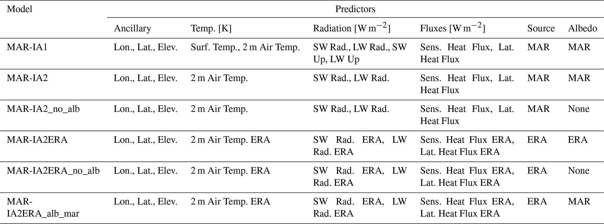
To broaden applicability, we constructed a second dataset using similar predictors but sourced from ERA5 and reprojected to the MAR grid (MAR-IA2ERA). This enables use of MAR-IA by the wider scientific community without requiring MAR forcing. Predictor selection for MAR-IA2ERA was guided by correlation and SHAP based predictor – importance analysis from MAR-IA1, retaining variables such as surface and 2 m air temperature, downwelling and upwelling shortwave/longwave radiation, and sensible and latent heat fluxes. Sublimation was excluded due to its minor role in Greenland (Lenaerts et al., 2012).

We examined the value distributions of the predictor variables using kernel density estimates (Fig. 2). In general, for training ML models, predictor distributions that are not overly concentrated within narrow value ranges can help reduce bias toward dominant portions of the data distribution. From Fig. 2, we observe that the predictor distributions are generally broad, although several variables are clearly non-Gaussian. The purpose of Fig. 2 is to compare the overall distributional shapes of the predictors rather than to characterize tail behavior in detail. Log–log transformations did not yield a significant improvement in accuracy, so no scaling was applied. We also studied the correlation among predictors (Fig. 3). Highly correlated predictors do not add substantial independent information to the training. They can also affect the attribution analysis, since variables with similar roles may be treated as separate predictors. Hence, to mitigate multicollinearity, we removed highly correlated predictors. Specifically, we identified strong relationships between 2 m air and surface temperature (r∼0.90). We dropped surface temperature because it saturates at 0 °C during melt, whereas air temperature retains variability and may still provide information on melting. Upwelling shortwave and longwave radiation were also removed. The remaining predictors showed weak correlations with meltwater production. Based on these criteria, we defined MAR-IA2 (Table 1), a refined MAR-only dataset excluding surface temperature and upwelling radiation fields.

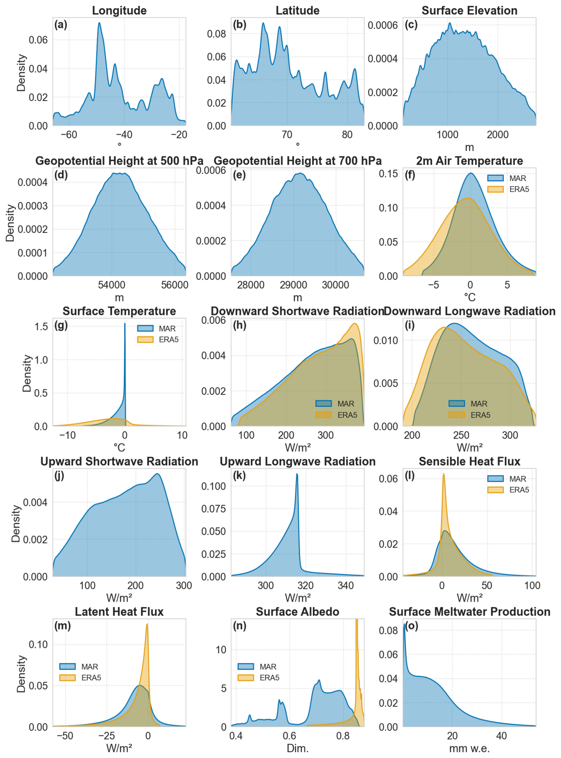
Figure 2 Distributions of MAR (blue) and ERA-5 (yellow) variables used for training the different models in this study.

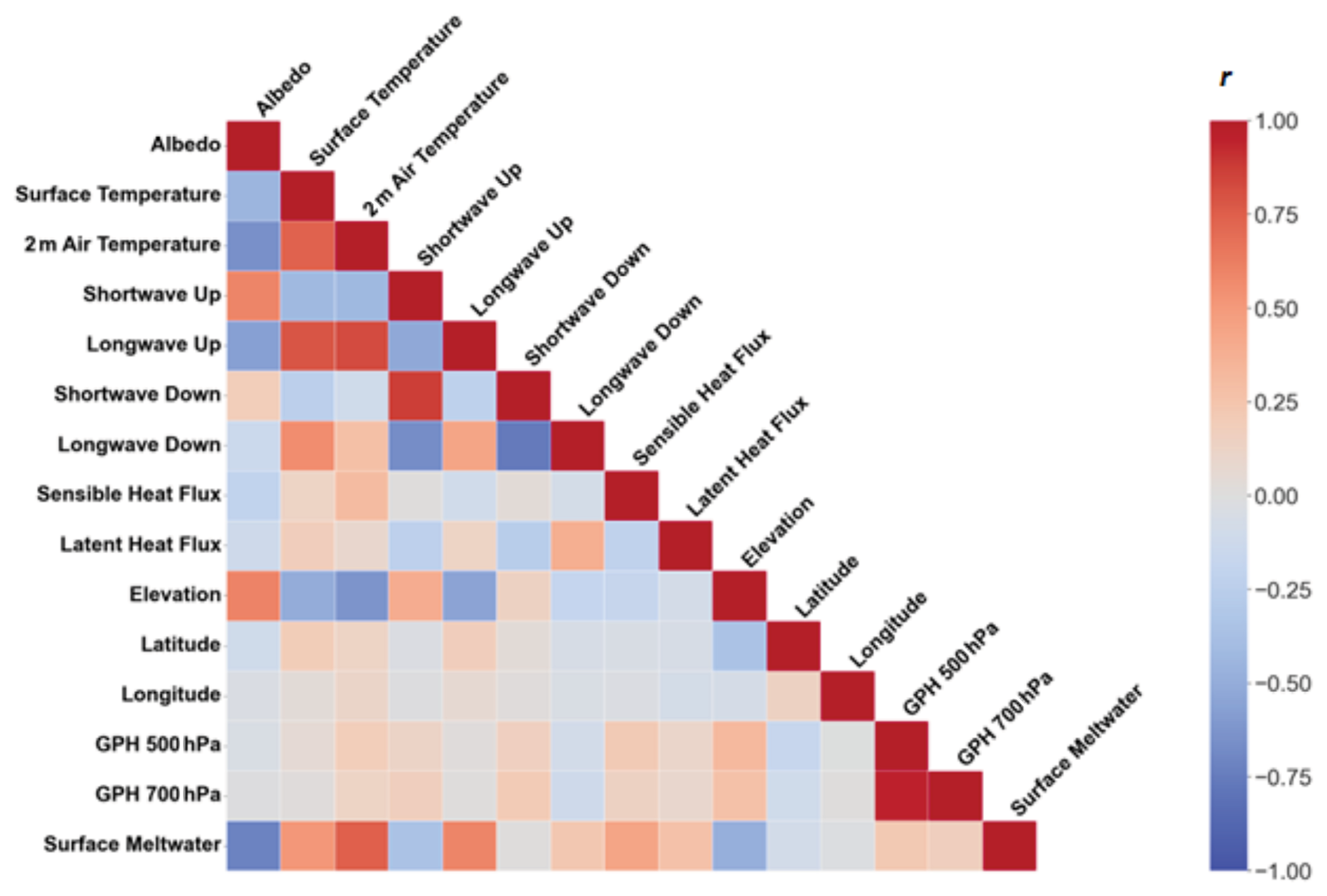
Figure 3 Heatmap of correlation coefficient (r) between the predictors and the predictand for the datasets used in the models' training.

We also evaluated the distribution of ERA variables vs. those obtained with MAR, to assess their differences and address the potential impact on the emulator's performance. Figure 4 also shows the distribution of summer mean values for ERA predictors. While several variables within MAR and ERA show general agreement in their distribution and magnitude, differences exist for shortwave radiation and sensible heat flux. The largest discrepancy is observed in the case of albedo. In this case, ERA exhibits minimal spatial variability (Fig. 4), with values around 0.8. We expect this to have an impact on the model's performance, in view of the importance of albedo on surface melting. To assess this, we trained models without albedo and tested a variant in which ERA albedo was replaced with MAR albedo.

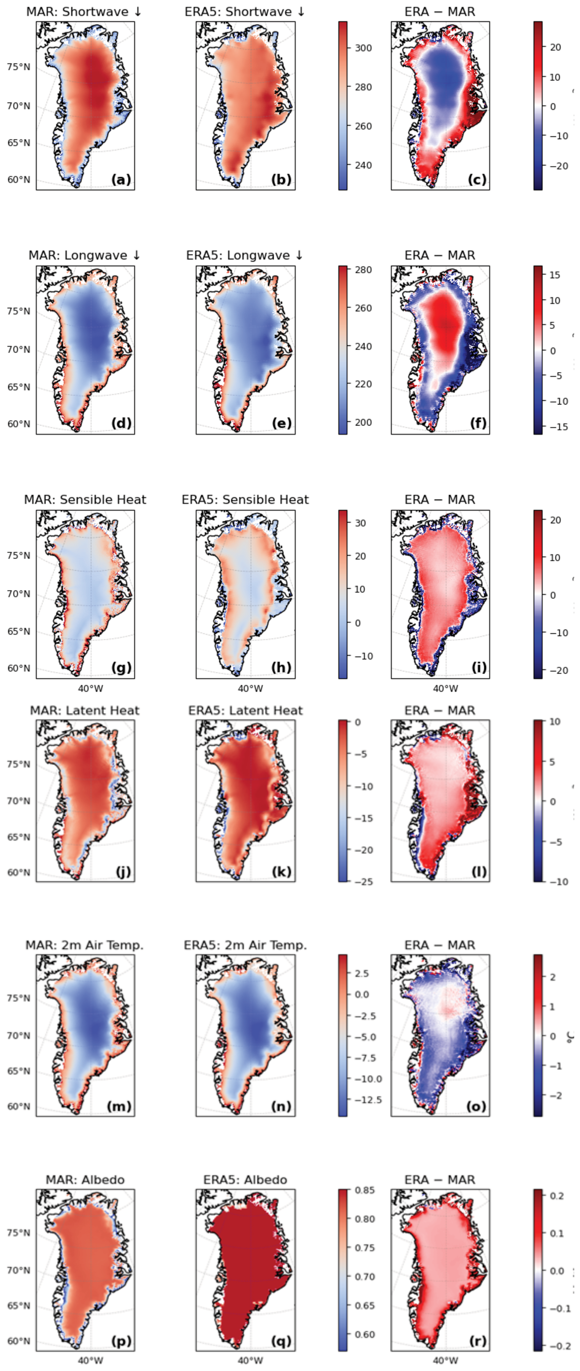
Figure 4 1979–2024 summer (June–July–August, JJA) averaged values for the predictors used in the models' training (left and center columns) and differences between the MAR and ERA-5 values (right column).

2.5 Hyperparameter optimization

Hyperparameter optimization refers to the process of selecting model parameters, such as learning rate, regularization strength, and tree depth, that are not learned during training but strongly influence model performance and generalization (Feurer et al., 2015). Common approaches include grid search, random search (Bergstra and Bengio, 2012), and Bayesian optimization (Snoek et al., 2012), the latter using probabilistic models to explore the parameter space efficiently.

For this study, we applied Bayesian optimization with five-fold cross-validation, in which the training data are divided into five subsets and the model is trained repeatedly using four subsets for fitting and one for validation, to tune a subset of key XGBoost parameters known to affect predictive accuracy (Chen and Guestrin, 2016). Bayesian optimization constructs a surrogate model of the cross-validated error and iteratively selects new candidates using an acquisition function that balances exploration of uncertain regions and exploitation of promising areas. This approach reduces the number of evaluations required to identify near-optimal settings. The search space was defined over the following discrete hyperparameter values: n_estimators = {100, 200, 500, 700, 1000, 1500, 2000, 2500}, max_depth = {2, 3, 5, 10, 15}, learning_rate = {0.05, 0.10, 0.15, 0.20}, min_child_weight = {1, 2, 3, 4} , and gamma = {0, 0.25, 0.5}. This corresponds to 1920 possible combinations in the full discrete search space. Using Bayesian optimization, we evaluated 50 candidate configurations (n_iter = 50) rather than exhaustively testing all combinations.

The optimization objective was to minimize mean squared error (MSE) across folds. We used the BayesSearchCV implementation from the scikit-optimize package (Head et al., 2018) to tune five XGBoost hyperparameters that jointly govern model capacity and regularization: n_estimators (number of boosting rounds) sets the overall number of additive trees (larger values can improve fit but also increase computation and, if not counterbalanced by regularization, may amplify overfitting); max_depth controls the depth of individual trees (deeper trees can represent higher-order feature interactions but tend to increase variance); learning_rate scales the contribution of each tree (smaller values typically promote smoother, more stable optimization); min_child_weight specifies the minimum summed instance weight required to create a new child node; finally, gamma defines the minimum loss reduction required to introduce an additional split. We performed hyperparameter tuning on the MAR-IA1 model, which uses all MAR variables, to maximize agreement with MAR outputs and provide a baseline for other configurations. Model performance is reported using the coefficient of determination (R²), which quantifies the fraction of variance explained by the model (higher is better); mean squared error (MSE), which measures the average squared deviation between predictions and observations (lower is better); root mean square error (RMSE); and bias, which represents the mean difference between predictions and ground truth, where values near zero indicate negligible systematic error. Starting from n_estimators = 100, performance was R²≈0.938, RMSE ≈ 1.082 mm w.e. d⁻¹, and bias $\approx -\mathrm{1.0}$ × 10⁴ mm w.e. d⁻¹. The global optimum occurred at n_estimators = 2500, max_depth = 15, min_child_weight = 4, learning_rate = 0.05, and gamma = 0, achieving R²=0.996, RMSE = 0.249 mm w.e. d⁻¹, and bias = 0.0002 mm w.e. d⁻¹. Beyond several hundred trees, the accuracy plateaued while the computational cost – particularly for SHAP-based attribution – increased substantially. As a compromise, we fixed non-iterative hyperparameters and used n_estimators = 500, yielding R²= 0.987, RMSE ≈ 1.344 mm w.e. d⁻¹, and bias $\approx -\mathrm{0.0002}$ mm w.e. d⁻¹. This configuration retained most of the accuracy while keeping training and interpretation tractable and was applied consistently across all models.

3 Results

3.1 Models' performances

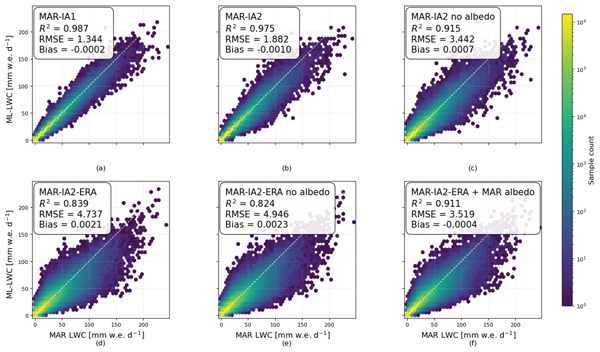
All machine-learning (ML) models were developed using a randomly shuffled split of the full dataset. Specifically, 70 % of the samples were used for training, 20 % for validation, and 10 % for testing. This split is a widely adopted heuristic in ML, providing sufficient training samples while retaining independent validation and performance assessment subsets (Gholamy et al., 2018; Sivakumar et al., 2024; Li et al., 2023; Xu et al., 2024). Figure 5 presents scatterplots of liquid meltwater production in the uppermost metre (here used as a predictor) obtained from the original MAR model (x-axis) with those obtained from the ML emulators (y-axis). Training, validation, and test data are shown, respectively, as red, green, and blue dots. Test-set performance metrics are summarised in Table 2 using the coefficient of determination (R²), mean squared error (MSE), root mean squared (RMSE) and prediction bias. Table 2 also reports 95 % confidence intervals for RMSE and bias, which quantify uncertainty in these test-set performance estimates.

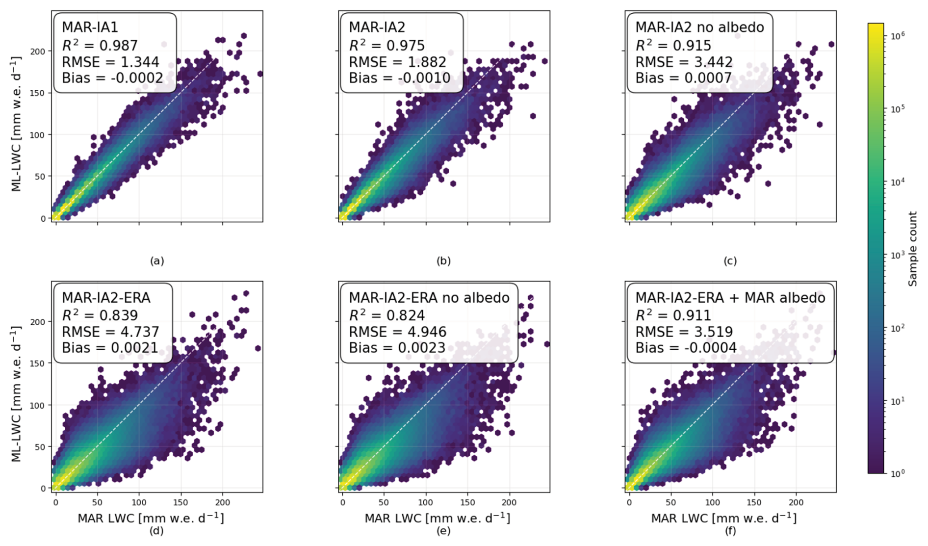
Figure 5 Scatterplot of the MAR (x-axis) and MAR-IA simulated (y-axis) surface meltwater production in the case of MAR-IA1 (a), MAR-IA2 (b), MAR-IA2_no_alb (c), MAR-IA2ERA (d), MAR-IA2ERA_no_alb (e), MAR-IA2ERA_mar_alb (f). Note only the test data statistics are reported and plotted.

Table 2 Test-set performance metrics (R², MSE, RMSE, bias, and 95 % confidence intervals for RMSE and bias) for each trained model using the predictor configurations described in Table 1.

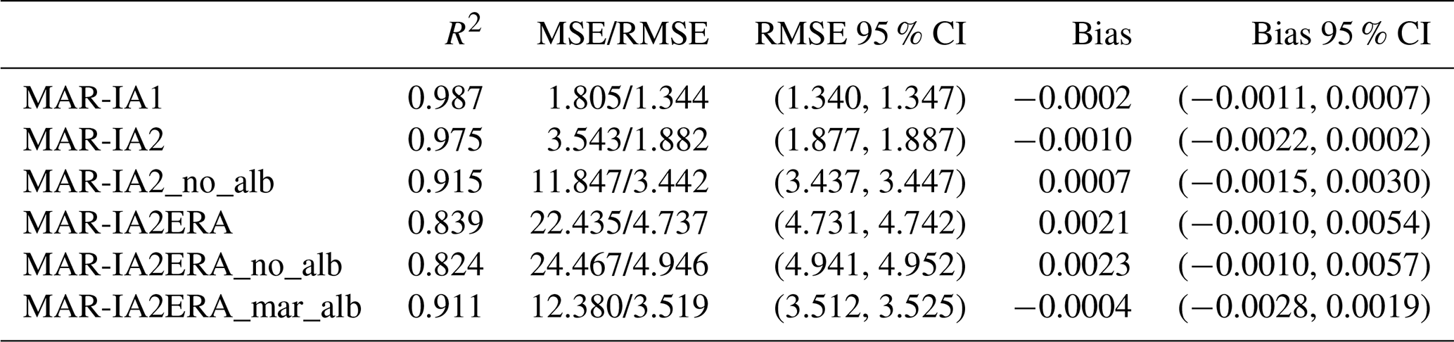
As expected, the MAR-IA1 model (Fig. 5a), which includes the full predictor set, achieves the highest accuracy (R² = 0.987, RMSE = 1.344 mm w.e. d⁻¹), with an low bias (−0.0002 mm w.e. d⁻¹). The narrow 95 % confidence intervals for RMSE and bias (Table 2) indicate stable test-set performance across the evaluated models. For comparison, an ordinary least-squares linear regression trained on the same predictor set achieved R² = 0.90 indicating a clear gain in predictive skill from the non-linear emulator. Excluding surface temperature and upwelling longwave and shortwave radiation (MAR-IA2) has little effect on R² (0.975) but results in a higher RMSE of 1.882 mm w.e. d⁻¹, reflected in the greater spread for low melt values (<20 mm w.e.; Fig. 5b). Using ERA-based predictors (MAR-IA2-ERA) further reduces performance (R² = 0.839, RMSE = 4.737 mm w.e. d⁻¹), with larger errors also concentrated at low melt rates (Fig. 5d). The small difference between MAR-IA2-ERA (Fig. 5d) and MAR-IA2-ERA-no_alb (Fig. 5e, where albedo from ERA is removed as a predictand) suggests a limited role of albedo in ERA-based configurations. This (as well as the deterioration in the ERA-based model's performance) is very likely due to the lack of spatial variability in the albedo product, as we anticipated in the previous section. Substituting ERA albedo with MAR albedo in the ERA dataset markedly improves accuracy (Fig. 5f), confirming the deterioration of the ML emulator because of the lack of granular information on albedo within the ERA product.

To assess sensitivity to temporal autocorrelation, we also performed a chronology-preserving experiment in which the models were trained on data up to 2014 and evaluated on data from 2015–2024. For MAR-IA2 and MAR-IA2-ERA, the resulting R² values were almost unchanged (0.970 and 0.838, respectively), indicating that the main performance conclusions are robust to this alternative split strategy.

The spatial distribution of mean annual meltwater differences between the ML emulator and MAR is shown in Fig. 6 for the MAR-IA2 and MAR-IA2ERA configurations. The domain-mean difference for MAR-IA2 is 0.015 mm w.e. yr⁻¹ with a spatial standard deviation of 0.182 mm w.e. yr⁻¹, while MAR-IA2ERA exhibits a larger mean difference of 0.125 mm w.e. yr⁻¹ and a spatial standard deviation of 0.310 mm w.e. yr⁻¹. For reference, the standard deviation of MAR meltwater production is 1.97 mm w.e. d⁻¹.

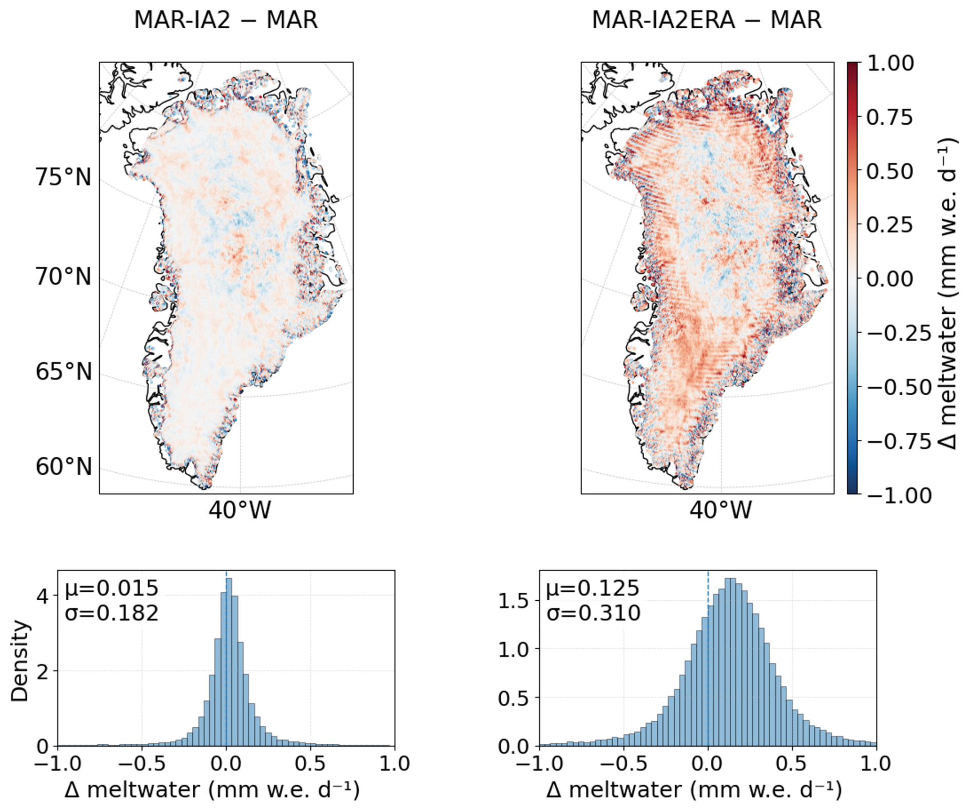
Figure 6 Mean difference in meltwater production between the machine-learning emulator and MAR for (left) MAR-IA2 and (right) MAR-IA2ERA configurations. Colors show the spatial distribution of the mean daily meltwater difference (ML − MAR) at each MAR grid point, obtained by averaging over all available days and years (1979–2024). The lower panels show the corresponding spatial distributions of the meltwater differences across the domain.

3.2 SHAP-based interpretation of emulator predictions

We applied SHAP to the trained emulators to interpret which predictors contribute most strongly to their meltwater predictions and to assess whether these learned relationships are broadly consistent with known melt processes. Here, SHAP values are interpreted as model-based attributions rather than direct causal effects. To reduce computational cost, we randomly selected a subset of 1000 points and repeated the SHAP analysis 10 times. Figure 7 shows the mean absolute SHAP values for the different models. Red denotes predictors with positive SHAP contributions, whereas blue denotes predictors with negative SHAP contributions. Error bars show the standard deviation across the 10 runs, reflecting attribution variability within this subsampling procedure.In the case of MAR-IA1 (Fig. 7a), 2 m air temperature shows the highest SHAP value (4.14 mm w.e. d⁻¹), followed by the downward shortwave radiation (3.94 mm w.e. d⁻¹), the albedo (3.57 mm w.e. d⁻¹) and the sensible heat flux (2.16 mm w.e. d⁻¹). In the emulator, higher albedo is associated with negative SHAP contributions, whereas higher shortwave radiation, 2 m air temperature, and downward longwave radiation are associated with positive SHAP contributions. Latitude and surface meltwater production are negatively correlated, meaning that meltwater production decreases from south to north. Surface (skin) temperature and meltwater production are negatively correlated. Nevertheless, the SHAP value in the case of surface temperature is relatively small and the relationship can be explained by the fact that the surface temperature saturates to 0 °C when melting occurs, hence providing no sensitivity to melting and showing negative values when no melting occurs.

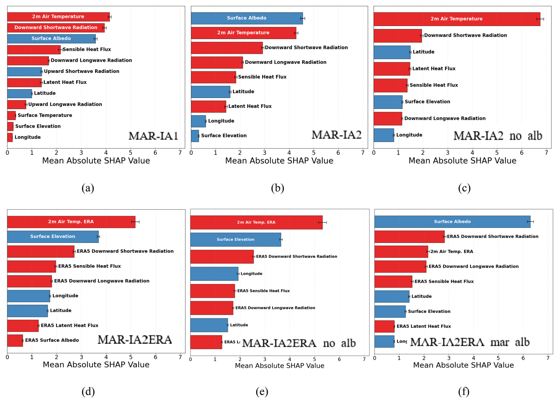
Figure 7 Mean absolute Shapley values obtained for the different models using the SHAP algorithm. Predictors that are negatively (positively) correlated with surface meltwater production are plotted as blue (red) bars.

The SHAP values for the MAR-IA2 (Fig. 7b) model are similar to those for MAR-IA1, with albedo, air temperature and shortwave radiation still being the dominant terms. The importance of albedo in the model is shown by the results from the MAR-IA2_no_alb model. Moreover, the results (Fig. 7c) show that, also in the case of an ML model without albedo, the model still assigns the largest SHAP importance to physically plausible predictors, consistent with current understanding of melt processes. Indeed, air temperature becomes the dominant driver, followed by latitude and shortwave/longwave radiation.

Similar results are obtained in the case of the MAR-IA2-ERA, where 2 m air temperature (5.17 mm w.e. d⁻¹), surface elevation (3.68 mm w.e. d⁻¹) and downward shortwave (2.71 mm w.e. d⁻¹) are the three predictors with the largest SHAP importance. We point out the model's lack of sensitivity to albedo, given the spatio-temporal granularity of this variable in the ERA product. This hypothesis is also supported by the results obtained with MAR-IA2ERA_no_alb. In this case (Fig. 7e), we observe that the SHAP values are only mildly affected by the removal of the albedo. Furthermore, Fig. 7f shows the SHAP values obtained with the MAR-IA2ERA_mar_alb model, which uses all ERA-5 variables as predictors with the exception of albedo, which comes from MAR. In this case, the results are consistent with those obtained with the MAR-IA1 and MAR-IA2 models, with albedo gaining a dominant role in the emulator attribution.

3.3 Assessment of the ML model at selected sites

We also evaluated the performance of MAR-IA2 against the conventional MAR model at two well-established monitoring sites: the K-transect S6 station (Fig. 8a) and Swiss Camp (Fig. 8b), during the summer of 2012. These sites provide high-quality observational data, making them ideal benchmarks for assessing model accuracy. The comparison revealed strong agreement between MAR-IA2 and MAR in simulating surface energy fluxes, with only minor deviations across key variables, including net radiation, sensible heat flux, and latent heat flux. At the Swiss Camp station, the mean absolute difference between the machine learning model and MAR is 1.17 mm w.e. d⁻¹, with an RMSE of 1.52 mm w.e. d⁻¹, a maximum of 5.97 mm w.e. d⁻¹, and a standard deviation of 0.96 mm w.e. d⁻¹.The model performs comparably well at the K-transect S6 station, yielding a mean difference of 0.91 mm w.e. d⁻¹, an RMSE of 1.31 mm w.e. d⁻¹, a maximum of 6.54 mm w.e. d⁻¹, and a standard deviation of 0.93 mm w.e. d⁻¹.This result underscores the reliability of the ML-based emulator as a robust emulator for the MAR model. Peaks associated with key melt events are also well captured, as are the general magnitude and patterns of melt variability. For reference, near peak melt (top 20 percentile of melt), MAR-IA2 has a maximum absolute percentage error of 1.81 % at S6 station and 2.48 % at the Swiss camp site. Minor differences that do occur are generally modest lags or amplitude differences around peak melt events.

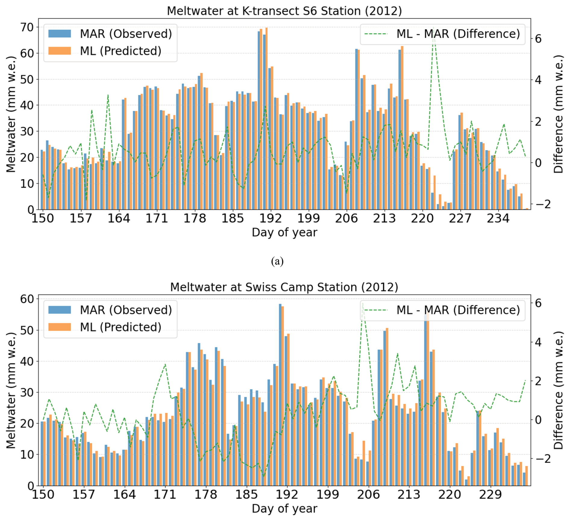
Figure 8 Comparison of daily MAR-IA2 Machine Learning Model and MAR Model Predictions at (a) K-transect S6 and (b) Swiss Camp Stations in Summer 2012.

4 Discussion

After assessing the skill of the MAR-IA emulator in reproducing MAR meltwater output, we turn to the SHAP analysis to examine which predictors the emulator relies on most strongly and how those emulator-based attributions vary spatially and temporally.

Figure 9 shows the summer (JJA) mean SHAP values for the (a) non-flux and (b) flux variables for the period 1979–2024 for the MAR-IA2 model. Linear trends are also reported as dashed lines with the same color as the corresponding variables. Our results show that the relative role of the 2 m air temperature has increased over the past decades (slope = 0.0081 yr⁻¹, p<0.01, Table 3). Shortwave radiation also shows a significant increase in its influence (0.0051 yr⁻¹, p≈0.01), reflecting the growing dominance of radiative forcing. Sensible heat flux displays a similarly strong and statistically significant positive trend (0.0043 yr⁻¹, p<0.01), pointing to enhanced turbulent heat transfer. Albedo shows summer values similar (in magnitude) to those obtained in the case of air temperature. However, in this case, the trend is small and not statistically significant. This is consistent with the recent albedo variability observed over Greenland (Feng et al., 2023). Latent heat flux exhibits a moderate but significant upward trend (0.0028 yr⁻¹, p≈0.03), suggesting a rising role of moisture-related surface processes, while longwave radiation shows no meaningful directional trend (p≈0.63). Among the non-flux variables, elevation shows a strong negative trend (−0.0016 yr⁻¹, p<0.01), indicating that low-elevation regions increasingly dominate the spatial pattern of melt variability. Latitude also shows a statistically significant negative trend (−0.0022 yr⁻¹, p<0.01), whereas longitude exhibits no significant change over time. We note that geographic variables such as latitude and longitude should not be interpreted as direct physical melt drivers. Rather, within the emulator they may act as spatial proxies for regional gradients or unresolved covarying conditions. As a further example of the relationships between SHAP values and the surface energy balance quantities, Fig. 10 shows the distribution of the averaged summed SHAP values, albedo and the MAR predicted meltwater for the years 1992 and 2012. These two years are characterized by opposite conditions in terms of surface melting, with 1992 being a low year, as a consequence of the Mount Pinatubo eruptions, and 2012 being an extremely high year in terms of meltwater production (e.g., Nghiem et al., 2012).

Table 3 Trend (per year) of the mean summer Shapley coefficients, together with the R² of the linear regression used to estimate each trend.

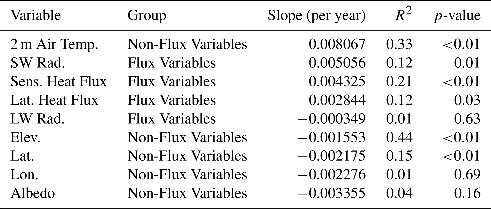
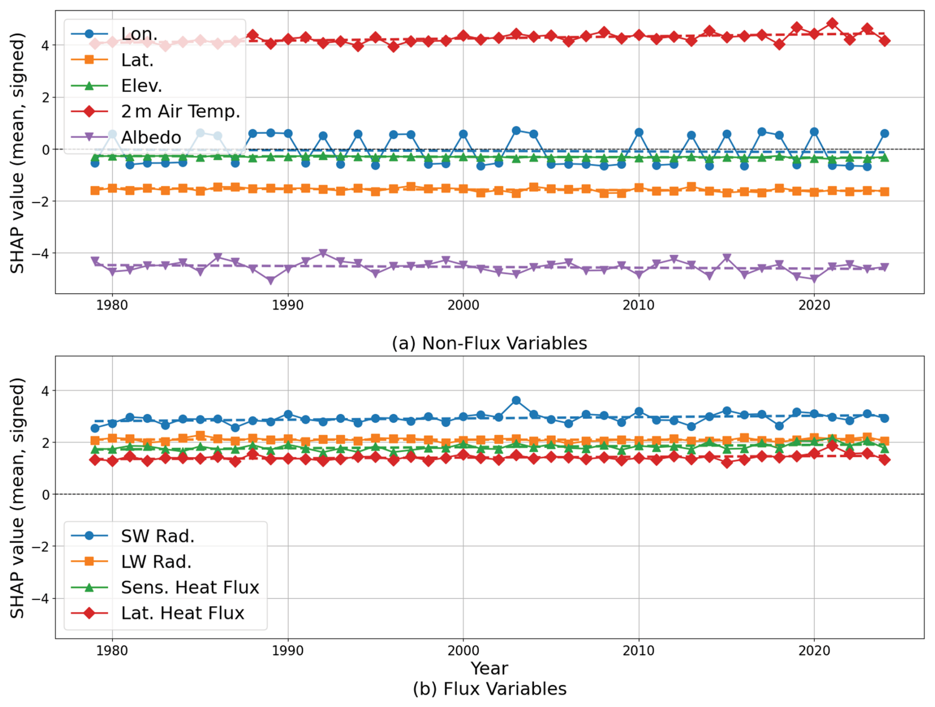
Figure 9 Summer (JJA) mean Shapley values for the (a) non-flux and (b) flux variables for the period 1979–2024. Linear trends are reported also as dashed lines with the same color as the corresponding variables. Note this is for MAR-IA2.

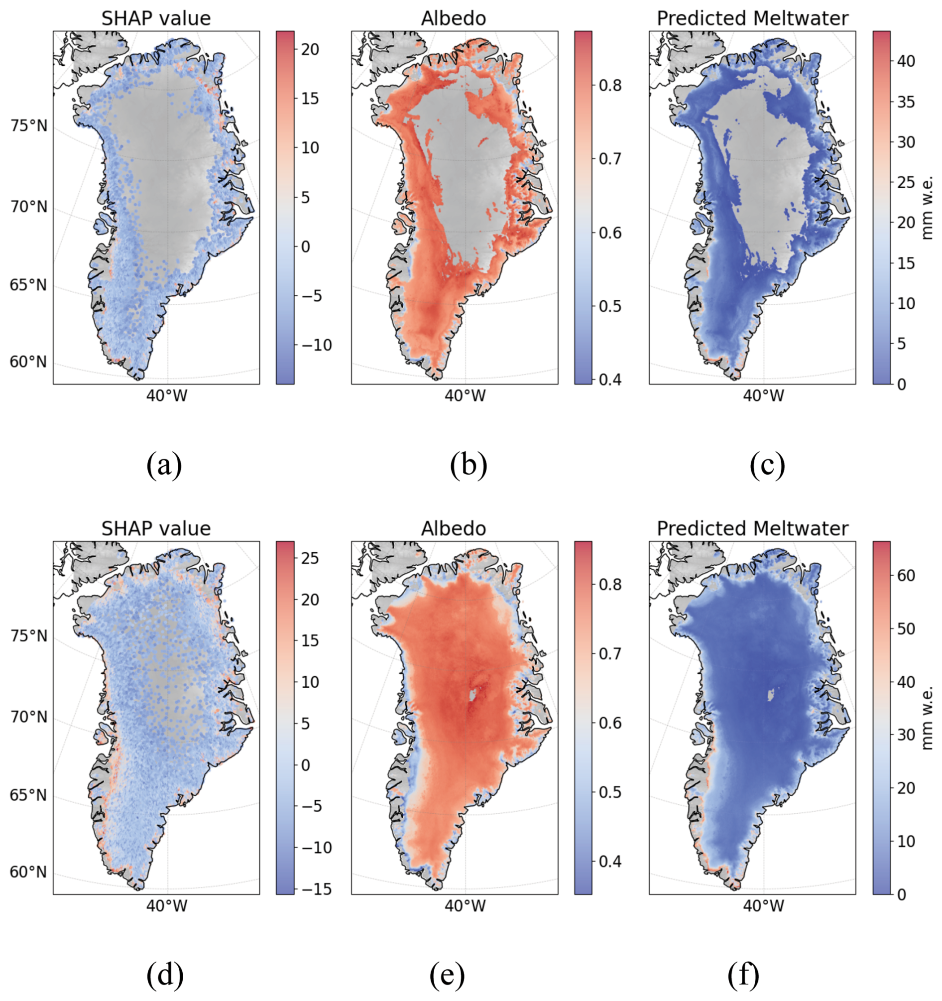
Figure 10 Summer-averaged spatial distribution of Shapley (a, d), albedo (b, e) and ML-estimated meltwater (c, f) for the 1992 (a, b, c) and 2012 (d, e, f) for the MAR-IA2 model.

To better understand the relative role of drivers on surface melting and explore the potential of the MAR-IA2 emulator, we performed SHAP analysis for different elevation bands (Fig. 11). Specifically, we divide the ice sheet into three elevations bands, 0–1000, 1000–2000 and above 2000 m. Our choice of the elevation bands is partially driven by the elevation of the equilibrium line altitude (ELA, e.g., where runoff equals accumulation), which has been estimated to be fluctuating between 1200 and 1500 m. Our results in Fig. 11a shows that for areas between 0 and 1000 m and those between 1000 and 2000 m the largest SHAP contributions remain associated with albedo, air temperature, and downward shortwave radiation. This is similar to the results obtained when considering the whole ice sheet. A difference between the two elevation bands is that for areas at lower elevations the magnitude of the mean SHAP values is higher (∼ 6 mm w.e.) than for the region between 1000 and 2000 m (∼ 4 mm w.e.). For this region (Fig. 11b), albedo becomes the dominant driver, though the SHAP values are comparable to those for air temperature. For areas above 2000 m (Fig. 11c), downward longwave radiation becomes the third most important predictor in the SHAP ranking, still after albedo and surface temperature. This is consistent with recent studies (Nghiem et al., 2012; Neff et al., 2014) showing that the intrusion of warm, moist air to the top of the ice sheet was responsible for surface melting.

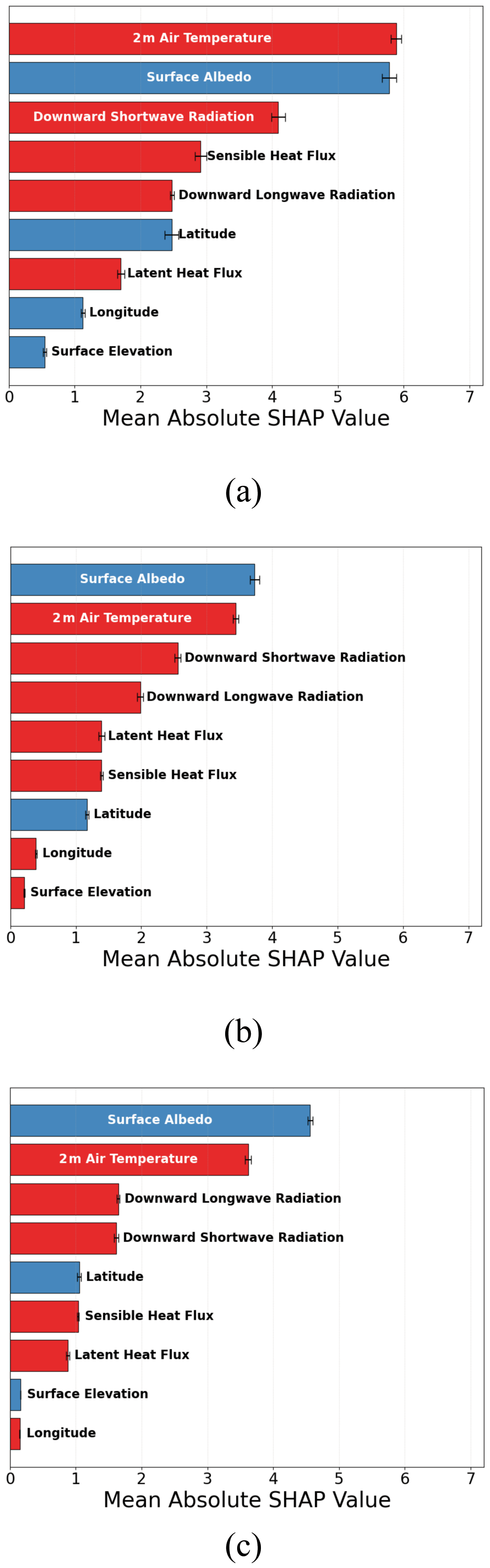
Figure 11 Mean absolute Shapley values obtained for the MAR-IA2 model for areas (a) below 1000 m, (b) between 1000 and 2000 m nd (c) above 2000 m.

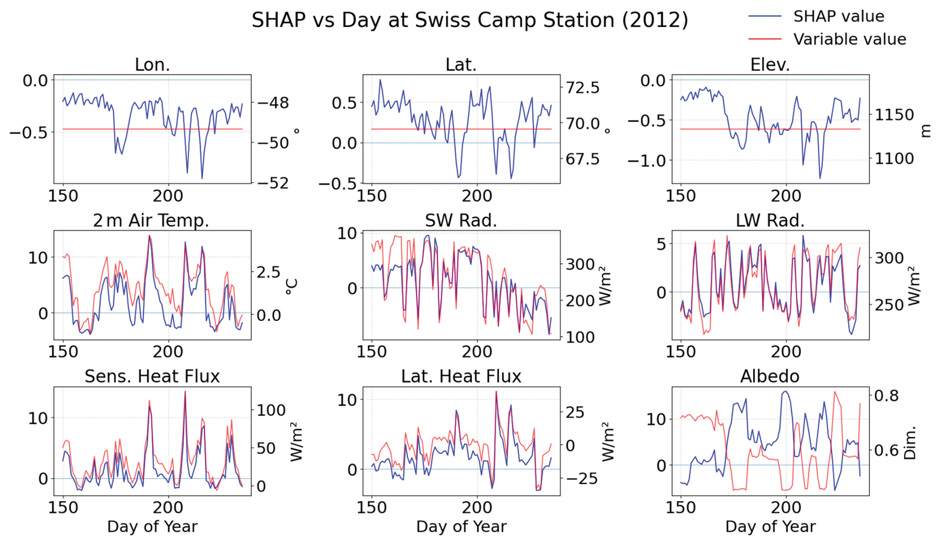
Lastly, in Figs. 12 and 13 we show the temporal evolution of daily SHAP values at the K-transect S6 (Fig. 12) and Swiss Camp (Fig. 13) stations for the year 2012 for the predictors used in MAR-IA2. The figures also show the – on the left y-axis – the corresponding daily values of the predictors. Over the course of the season, the magnitude and sign of individual SHAP values fluctuate, reflecting changing physical conditions and the covariate dependency of melt drivers. Most SHAP attributions covary with the predicted meltwater value, and the relationship between SHAP and predictand values changes dynamically. Obviously, in these examples, latitude, longitude, and elevation remain the same, though their relative ratios fluctuate. Albedo shows a less evident relationship between the SHAP value and the predictand, due to the saturation of low albedo values during intensive and prolonged melting periods. In the case of the K-transect, for example, we observe the albedo values of ∼ 0.4 lasting for several days starting at the end of May (day 180). Despite the albedo value remaining relatively constant, the SHAP values fluctuate to account for the changing conditions due to the variability of other forcings. Similar considerations apply to Swiss Camp (Fig. 12).

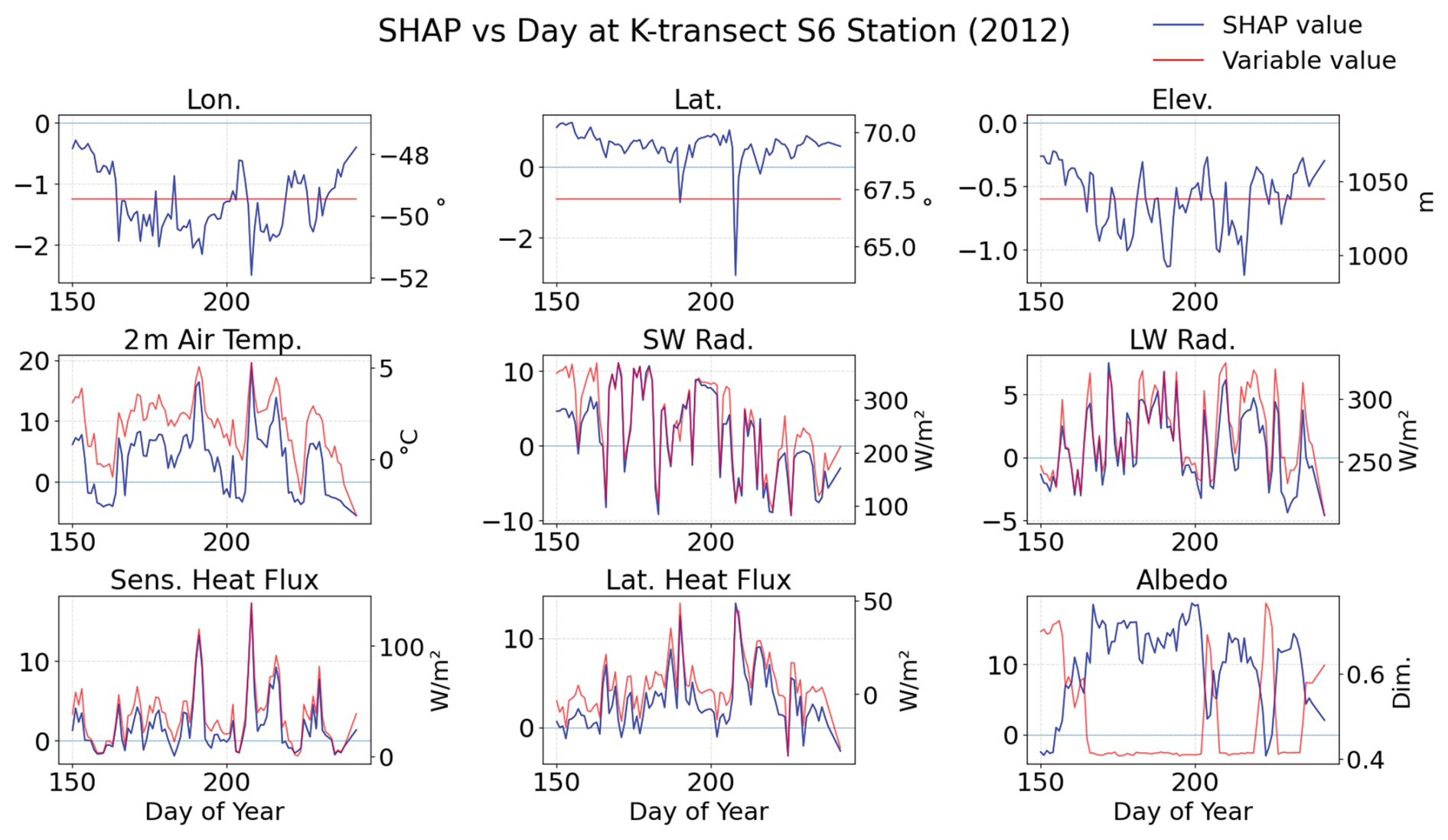
Figure 12 Daily Shapley values for the different predictors obtained from the model MAR-IA1 and associated trends (dashed red line) for the pixel containing the K-transect S6 station.

Figure 13 Same as Fig. 8 but for the Swiss Camp location.

5 Conclusions

In this study, we introduced MAR-IA, a machine learning (ML) emulator designed to replicate surface meltwater production over the Greenland Ice Sheet (GrIS) as simulated by the MAR regional climate model (Fettweis et al., 2017). MAR-IA leverages XGBoost, a tree-based ML algorithm, trained on MAR outputs from 1979–2024 using predictors such as albedo, air temperature, radiative fluxes, and turbulent heat fluxes (MAR-IA1). Predictor selection was guided by both physical relevance and statistical analysis. Initially, we considered all variables associated with the surface energy balance, including albedo, surface and near-surface temperatures, shortwave and longwave radiation, and sensible and latent heat fluxes. Highly correlated variables, such as surface temperature and upwelling radiation fields, were removed to avoid redundancy and multicollinearity (Kim, 2019), which can obscure feature importance and inflate variance to train an alternative model (MAR-IA2). A third configuration, MAR-IA2-ERA, was trained on ERA5-based predictors (Hersbach et al., 2020) to facilitate wider usability, although its performance is affected by the limited spatial variability of ERA's albedo product. Experiments substituting ERA albedo with MAR albedo demonstrated substantial improvements in accuracy, underscoring the critical role of albedo in meltwater prediction and the need for improving albedo estimates within the ERA dataset.

Performance assessments reveal that MAR-IA1 achieved high agreement with MAR outputs on the test set, with R²=0.987 and RMSE = 1.344 mm w.e. d⁻¹, confirming the emulator's fidelity. MAR-IA2 retains strong performance with R²= 0.975 and RMSE = 1.882 mm w.e. d⁻¹, despite using fewer predictors. In contrast, MAR-IA2-ERA shows reduced accuracy, with R²=0.839 and RMSE = 4.737 mm w.e. d⁻¹, primarily due to ERA's lack of albedo representation. When MAR albedo replaces ERA albedo, performance improves markedly to R²=0.911 and RMSE = 3.519 mm w.e. d⁻¹. These results demonstrate that while ERA-based models enable broader applicability, predictor quality – particularly albedo – remains essential for accurate meltwater emulation. Overall, MAR-IA provides a computationally efficient alternative to physically based models, supporting large-scale simulations and long-term attribution studies.

SHAP provides a useful framework for interpreting the predictions of the MAR-IA emulators by quantifying the contribution of each input predictor to the model output. In this study, we used SHAP to assess which predictors the emulator relies on most strongly and whether those learned predictor–melt relationships are broadly consistent with current physical understanding of surface melt over Greenland. The analysis showed that albedo, downward shortwave radiation, and 2 m air temperature consistently receive the largest SHAP importance, in agreement with established knowledge of the surface energy balance. At the same time, we interpret these results as model-based attributions, not as direct causal proof. In particular, SHAP values depend on the trained emulator and can be influenced by remaining correlations among predictors. We therefore view the SHAP analysis as a physically informed interpretation of the emulator, rather than a replacement for direct process-based diagnosis from MAR itself.We studied how the relative role of the different predictors has been changing over the past decades over Greenland. We found an increasing contribution of 2 m air temperature, together with a rise in the influence of downward shortwave radiation, being consistent with a melt regime progressively dominated by atmospheric warming and enhanced radiative forcing. In parallel, the growing role of sensible heat flux might point to strengthened turbulent heat transfer as a co-evolving driver of melt variability. Albedo remains an important control on surface melt, with a summer mean influence comparable in magnitude to that of air temperature. However, its long-term trend is small and not statistically significant. This is consistent with recent studies showing substantial Greenland albedo variability, but not necessarily a simple monotonic increase in its contribution to melt over time (Feng et al., 2023). The comparison of SHAP summer maps for low-melt (1992) and extreme-melt (2012) years further illustrates how the emulator and SHAP decomposition can provide physically interpretable results across regimes and extremes: 1992 reflects externally forced radiative suppression following the Mount Pinatubo eruption, whereas 2012 captures the compounded influence of strong melt-favorable energy inputs and feedbacks associated with a well-documented pan-Greenland melt episode (Nghiem et al., 2012).

Attribution stratified by elevation bands further underscored that “dominant drivers” are not spatially uniform. While albedo, air temperature, and shortwave radiation remain primary controls below 2000 m, their absolute contributions are stronger at the lowest elevations, consistent with higher melt sensitivity. Above 2000 m, downward longwave radiation becomes comparatively more important. This supports the interpretation that episodic intrusions of warm, moist air, and the associated enhancement of longwave radiation, can be critical for high elevation melt events. This is again consistent with prior evidence from extreme years such as 2012 (Nghiem et al., 2012). Finally, station-scale daily analyses at K-transect S6 and Swiss Camp in 2012 demonstrate that melt drivers are highly state-dependent. SHAP values change sign and magnitude through the season as boundary-layer structure, radiative conditions, and surface state co-evolve. The results concerning albedo values and their SHAP attribution during prolonged melt – reflecting albedo saturation at low values – highlight how the MAR-IA model captures marginal contributions in context, not merely the instantaneous magnitude of a variable.

The development of MAR-IA opens several avenues for future research and practical applications. First, expanding the emulator to include additional target variables or predictors such as snowpack properties, cloud microphysics, and atmospheric circulation indices could improve its ability to capture complex melt dynamics under changing climate conditions and offer an insight into the relative role of dynamic and thermodynamic drivers. Our current work is to export the model to other regions – such as Antarctica, the Himalaya, and the European Alps – as well as extend our method to SMB. We also suggest that the low computational cost of the ML emulators allows running synthetic experiments to quantify uncertainty, conducting sensitivity experiments, and coupling the emulator with other models, focusing, for example, on modelling the total mass loss of the Greenland and Antarctic ice sheets, such as the ISSM (Larour et al., 2012). Moreover, the emulator offers a practical alternative when the full MAR atmospheric model cannot be run. MAR requires lateral boundary forcing over Greenland with meteorological variables at several vertical levels, and these inputs are not always available with sufficient completeness for historical reconstructions or future climate simulations. The emulator circumvents this requirement by predicting meltwater directly from a reduced set of atmospheric and surface predictors, without integrating the full atmospheric model. Its use for past or future applications is therefore promising, but should be restricted to conditions that remain within, or close to, the range represented in the training data, with further validation needed for true extrapolative cases.Tools like MAR-IA can accelerate large-scale attribution studies, sensitivity experiments, and multi-model intercomparisons, promoting collaborations across glaciology, climate science, and machine learning fields. We are not arguing that fundamental climate models and physically based knowledge of processes should be fully replaced by machine learning tools or methods. On the contrary, we argue that the real benefits arise from the proper alignment of fundamental research leading to the understanding of the processes and feedbacks driving the observed processes and machine learning tools. This can accelerate the pace of discovery and enable model-interpretation analyses via, for example, SHAP-based attribution, helping summarize emulator behavior at lower computational cost and supporting synthetic experiments that improve understanding of past changes while refining future estimates.