Svalbard glacier calving front changes from the 1930s to the 1970s from archived satellite and aerial images

We obtained calving front positions of 171 Svalbard tidewater glaciers from archived satellite imagery. We used early Landsat images from 1976–1978 as well as declassified intelligence satellite photographs from 1962–1963. To support the analysis of these calving fronts, we also used historical aerial images from 1936–1938. During our study period between 1936–1978, we estimate an average glacier retreat rate of $\mathrm{27.3}\pm \mathrm{3.0}\mathrm{m}{\mathrm{yr}}^{-\mathrm{1}}$. This corresponds to an average retreat of approximately 1 km for Svalbard tidewater glaciers during this period. By multiplying the retreats by the glaciers' widths, we estimate the cumulative area loss rate to be $\mathrm{17.0}\pm \mathrm{2.5}{\mathrm{km}}^{\mathrm{2}}{\mathrm{yr}}^{-\mathrm{1}}$, which is slightly lower than the estimates found in the existing literature for the periods 1985–2023 and 2000–2020, and consistent with climatic trends from reanalysis data. Looking at individual glaciers, we identify and discuss 15 significant advance events. For four of them, our study provides additional information to current knowledge. We have discovered one undocumented surge – we show evidence that Emmabreen has surged between 1936–1963. We have also narrowed down the time windows of two previously known surges: the surge of Allfarvegen to between 1976–1978 (previously reported to have happened between 1970–1980), and the surge of Stonebreen to between 1936–1963 (previously reported between 1936–1971). We also show that Schweigaardbreen and Fonndalsbreen have advanced 400 and 541 m, respectively, between 1938–1976. We discuss the potential future uses of our dataset, consisting of georeferenced satellite images used in our study as well as digitized calving fronts, which is freely available for future research.

1 Introduction

1.1 Svalbard glaciers

Svalbard is a Norwegian archipelago located in the high Arctic, between 74 and 81° N latitude, and 10 and 34° E longitude. About 57 % of the archipelago is covered by ice; the Randolph Glacier Inventory version 7 (RGI; RGI 7.0 Consortium, 2023) inventoried 1666 glaciers on the archipelago, among which 196 terminate in the sea, all of which seem to be grounded (Hagen et al., 1993). Many Svalbard glaciers have a history of surging, meaning that their flow velocities can dramatically increase for a short period of time (typically 1–10 years). The climate, basal rheology, and glacier geometry of typical Svalbard glaciers seem especially favorable for surging, and the archipelago is one of the world's hotspots for surge activity (Sevestre and Benn, 2015). Among Svalbard tidewater glaciers, 139 are of surge-type (Harcourt et al., 2026).

Globally, glaciers are an important component of the climate system. They are a freshwater storage, and their mass loss can dramatically influence sea-level rise (SLR). Worldwide, glaciers are expected to lose 26 %–41 % (for mean temperature increase projections of +1.5 to +4 °C, respectively) of their mass by 2100, compared to 2015 (Rounce et al., 2023). In the Arctic, glacier mass loss contributes to changing the surface albedo, which amplifies global warming through positive local and regional feedbacks (Manabe and Wetherald, 1975). A better understanding of Svalbard glacier change is therefore crucial to assess their future evolution and their impact on the climate system.

1.2 Usage of historical aerial images

Several aerial photograph mapping campaigns have been carried out over Svalbard in the past century. Liestøl (1969) used historical photographs and written observations to produce an inventory of past glacier surges, and identified possible future surges. Geyman et al. (2022) took advantage of aerial images from 1936–1938 to generate a DEM of the archipelago, used to investigate historical mass balance changes of Svalbard glaciers in a 70-year time span. They discovered a strong correlation between the temperature and the mass loss rate: a 1 °C increase in mean summer temperature corresponds to an area-normalized mass balance of $-\mathrm{0.28}\mathrm{m}\mathrm{w}.\mathrm{e}.{\mathrm{yr}}^{-\mathrm{1}}$. They also predict a doubling of mass loss by 2100, using a space-for-time substitution. Nuth et al. (2010) compared a variety of DEMs produced from different aerial campaigns to calculate Svalbard glacier elevation changes and contribution to SLR between the 1960s and the 2010s. They calculated a volume change of $-\mathrm{0.36}\pm \mathrm{0.02}\mathrm{m}\mathrm{w}.\mathrm{e}.{\mathrm{yr}}^{-\mathrm{1}}$, corresponding to a SLR of 0.026 mm yr⁻¹.

1.3 Usage of Declassified Intelligence Satellite Photographs (DISP)

Since 1995 and the declassification of 860 000 US military intelligence satellite photographs from the 1960s and 1970s, it has been possible to extend the time series of satellite remotely sensed glacier data. KH-4, 4A and 4B CORONA (cf. Sect. 2.2.1) photographs have been used for historical studies, especially in archaeology (Galiatsatos, 2004; Goossens et al., 2006) and more recently in glaciology (Ghuffar et al., 2022; Cooper et al., 2022; Racoviteanu et al., 2022). Cooper et al. (2022) used these images along with other sources of historical data for the study of surface mass balance (SMB) and frontal advance/retreat of outlet glaciers in the eastern margin of the Greenland ice sheet and their responses to air and ocean temperature changes. Racoviteanu et al. (2022) used orthocorrected CORONA stereo-images to produce digital elevation models (DEMs) of the Mansalu region of Nepal, and compared them to recent sources of data to study glacier SMB.

KH-5 ARGON (cf. Sect. 2.2.1) images have also been used for historical studies. Kim et al. (2001) used KH-5 ARGON images to map the ice shelf margins along Queen Maud Land, Antarctica, and compared them to more recent observations. Wang et al. (2016) created an orthocorrected version of ARGON images over the Larsen Ice Shelf (Antarctica), and discovered that the acceleration that led to the collapse of Larsen B happened earlier than previously thought. Ye et al. (2017) used these images to produce a regional DEM of the Antarctic ice sheet. There is no published study using declassified intelligence satellite photographs (DISP) on Svalbard, despite the availability of several CORONA and ARGON images.

1.4 Usage of early Landsat images

The MultiSpectral Scanner (MSS) instrument equipped Landsat 1–5, and was in use between 1972–1999 (and was briefly turned back on in 2012–2013), enabling retrieval of glacier area changes. For example, Williams (1987) successfully used two Landsat MSS images to measure the area of Iceland's largest ice cap (Vatnajökull) and to inventory 38 of its outlet glaciers. Yavaşlı et al. (2015) used Landsat MSS, along with other types of multispectral satellite data, to calculate the area change of glaciers in Turkey. Landsat MSS images have also been used in Svalbard for glacier studies. Dowdeswell (1984) used Landsat MSS images to map the ice cap margins of Nordaustlandet and compared them to maps from that time. He discovered that revisions of these maps were necessary, particularly on the East coast and at certain outlet glacier margins. He also mapped the snow line position and the basal melting through the observation of sediment plumes offshore. Hagen et al. (1993) finally, used Landsat 3 images, among other sources of data, to produce an inventory of Svalbard glaciers and report all known surge events in Svalbard. They documented the type, area, activity, and geometry of every Svalbard glacier larger than 1 km².

Automated glacier mapping techniques using band ratios (Hall et al., 1987; Rott, 1994; Bayr et al., 1994) and the normalized difference snow index (NDSI; Hall et al., 1995) are not applicable to Landsat MSS images because of the lack of a SWIR band, which therefore need to be processed manually. Deep-learning approaches allow overcoming this limitation (e.g. Li et al., 2024). Li et al. (2024) used Landsat, Terra-ASTER and Sentinel-2A/B multispectral images, as well as Sentinel-1A/B images to train a deep learning model that produced a dataset of 124 919 glacier calving fronts for 149 marine-terminating glaciers in Svalbard between 1985–2023. Li et al. (2025) analyzed this dataset and observed seasonal cycles in front positions, with a several-month lag between peak retreat on Spitsbergen East and West coasts. Their observations are consistent with regional ocean warming patterns. After removing the seasonal variability, they calculated marine-terminating glaciers have globally retreated during the study period, with a rate of 23.78 km² yr⁻¹. Li et al. (2024) and Li et al. (2025) provide a detailed historical monitoring of Svalbard glacier calving fronts. However, early Landsat images (Landsat 1–3) were not used in the production of the final dataset.

The objective of this study is to bridge the gaps between past observations of Svalbard glaciers, by retrieving glacier calving fronts from DISP (1962–1963) and Landsat (1976–1978) images, and comparing the observations to historical aerial image calving front data (1936–1938, Geyman et al., 2022). In particular, this is the first study using DISP over Svalbard. It aims at comparing the front positions to assess their cumulative retreat or advance between the late 1930s and 1970s, which is a good indicator of glacier area change; and to document possible surge events that occurred during this period.

2 Data and methods

2.1 1936–1938 aerial photographs

In 1936 and 1938, two aerial expeditions were led by the Norwegian geologist Adolf Hoel over Svalbard. During these expeditions, 5507 images were acquired, in order to produce topographic maps of Svalbard. These images have been used more recently to monitor elevation changes on Svalbard glaciers. Geyman et al. (2022) processed these images with a modern photogrammetric workflow, and produced an orthorectified mosaic (Fig. 1) and a DEM. They also produced an updated 1936–1938 glacier outline inventory, which is used in this study together with the new 1960s and 1970s measurements.

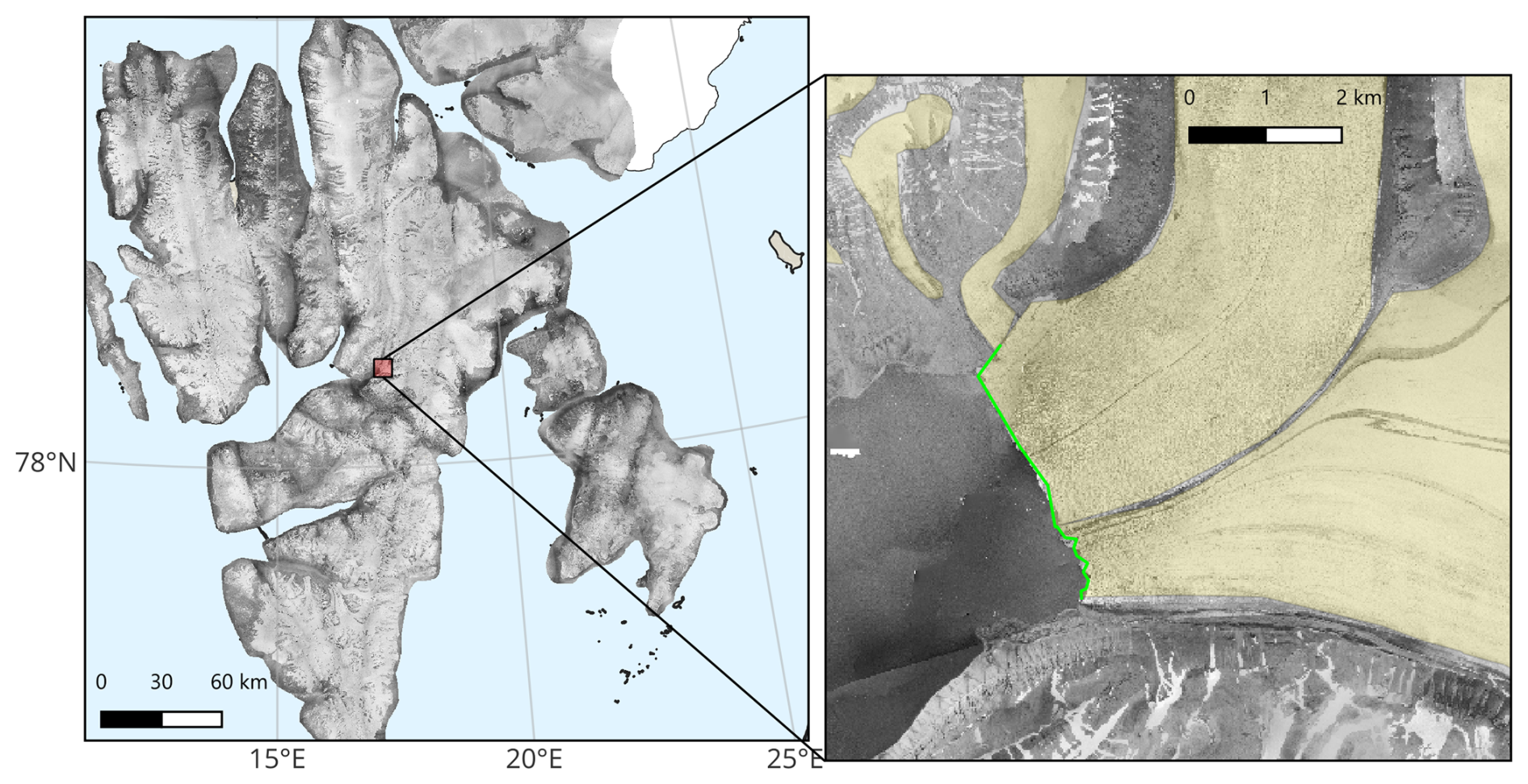
Figure 1 1936–1938 aerial images ortho-mosaic (left) and zoom on Tunabreen front (right). The yellow semitransparent areas represent the glacier outlines given by Geyman et al. (2022), and the green line represents the digitized glacier front. Background map: land and glaciers from TopoSvalbard © Norwegian Polar Institute; image credit: Norwegian Polar Institute.

2.2 DISP

2.2.1 DISP description

Between 1959–1984, the US intelligence agencies operated a series of reconnaissance satellites as part of a program called KeyHole (KH). The photographs were taken on panchromatic film, sent back to Earth in capsules that were retrieved mid-air by the US Air Force, and developed by the Central Intelligence Agency. In total, 1 660 000 satellite images were declassified in three stages in 1995, 2002, and 2011. Today, a copy of these films is conserved by the USGS, which can provide high-quality scans for USD 30 per frame at the time of writing (U.S. Geological Survey, 2018). Once the films are scanned, the images remain freely available on the EarthExplorer website. These images are highly valuable for historical studies and are referred to as DISP in the remote sensing scientific community.

In this study, we focus on eight KH-5 ARGON images, from missions 9034A (May 1962) and 9058A (August 1963). An example is given in Fig. 2. The satellite, whose altitude was between about 300 and 600 km, was equipped with a mapping camera, covering an area of about 540 km×540 km, with an approximate resolution of 140 m. The images were taken on 127 mm Kodak 3400 film, with a 76.2 mm focal length and an $f/\mathrm{2.5}$ aperture (Welch et al., 1982). The scan resolution is 7 µm (U.S. Geological Survey, 2018; Molnár, 2021), resulting in a ground-projected pixel size of about 30 m on the digital copy (note the resolution is 140 m but the sampling scale is finer). These images were taken in three different series (two on 16 May 1962, and one on 29 August 1963). Two consecutive images of the same series have an about 60 % overlap.

2.2.2 KH-5 ARGON images processing

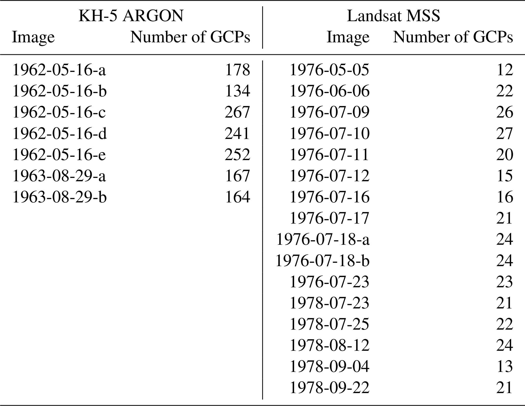
DISP are not georeferenced at all and present complex deformations that need to be corrected. For KH-5 ARGON images, deformations arise from terrain-induced parallax, Earth's curvature, and lens distortion. Additionally, long-term storage on film introduces random deformations in the images. Previous studies focused on orthorectifying these images, and including all the necessary corrections in the process (cf. Sect. 1). We attempted to implement the corrections explained in Molnár (2021), but the optimization process designed to retrieve the precise attitude parameters of the satellite failed. However, as we were only interested in obtaining glacier fronts that adjoin water surfaces, a full orthocorrection was deemed unnecessary and therefore not applied. Instead, we georeferenced the images using a 3rd degree polynomial transformation on QGIS, with 100–200 ground control points (GCPs) per image, to account for the complex geometry of KH-5 ARGON photographs. Table 1 (left) details the number of GCPs used for each image (cf. Appendix B2 for GCP maps and RMSE).

Table 1 Number of GCPs for KH-5 ARGON and Landsat MSS images georeferencing. For the sake of simplification, the images are identified by their date of acquisition. The full names are given in the Appendix (Tables A2 and A1).

2.3 Landsat MSS images

Landsat is an ongoing scientific Earth-observation program that started in 1972. Instruments equipped on the Landsat satellites have evolved over time to provide observations in more spectral bands and with higher spatial resolution. In this study, we focus on the early stages of the Landsat program, when the MSS was the main instrument onboard. U.S. Geological Survey (2020a) provides an overview of the Landsat MSS data products. We identified sixteen usable Landsat 2 and 3 (Level 1 Geometric-Systematic, L1GS) images of Svalbard from 1976 and 1978. Each image covers a 180 km×180 km area with a ground sample distance of 80 m, re-projected to a 60 m pixel size. These images are freely available on the U.S. Geological Survey (USGS) EarthExplorer website (https://earthexplorer.usgs.gov/, last access: 8 July 2026) and can be downloaded in GeoTIFF format. Figure 3 gives an example of two of these images.

We produced false color images from bands 7, 5, and 4 using the rioxarray Python package. The original geolocation was off by multiple kilometers, which required correction. To do this, we selected about 20 GCPs for each image (cf. Table 1) in QGIS using the Georeferencer tool and applied a 2nd degree polynomial transformation (cf. Appendix B2 for GCP maps and RMSE).

2.4 Front digitization

Once we had georeferenced the KH and Landsat images, we digitized tidewater glacier fronts. Given the small number of usable images, a single operator carried out this process manually in QGIS. Therefore, the accuracy of the front positions is, at best, the image resolution (60–140 m). On several Landsat images and on 1962 KH images, sea ice is present in the fjords, resulting in a lower accuracy. We delineated the fronts on every image on which they were visible (Figs. 3 and 2, right panel). Therefore, for several glaciers, multiple mappings from the same year are available and can be used to assess the positioning uncertainty. In total, we made 467 Landsat and 526 KH observations, for 185 calving fronts on 171 glaciers. For the aerial photographs, Geyman et al. (2022) had already digitized glacier outlines, and we simplified the shapefile containing the glacier polygons to extract only the tidewater glacier fronts. 169 front observations are included in this dataset (Fig. 1, right panel), covering all Svalbard tidewater glaciers, except the easternmost part of Nordaustlandet. Figure 4 shows the extent of the complete dataset.

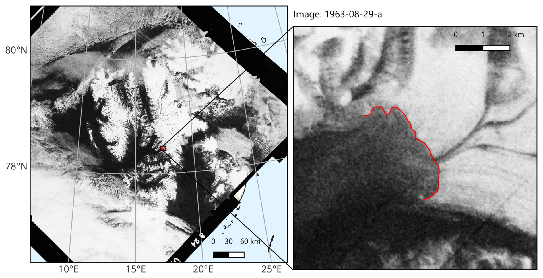
Figure 2 Example of KH-5 ARGON image (left) and zoom on Tunabreen front (right). The full image names are given in the Appendix (Table A1). The red line represents the digitized glacier front. Background map: land and glaciers from TopoSvalbard © Norwegian Polar Institute; image credit: U.S. Geological Survey.

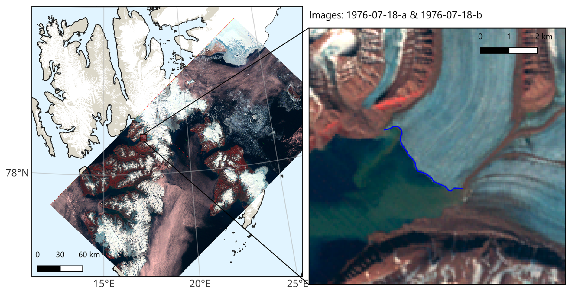
Figure 3 Example of a mosaic generated from two consecutively acquired Landsat MSS images (left), and zoom on Tunabreen front (right). The full image names are given in the Appendix (Table A2). The blue line represents the digitized glacier front. Background map: land and glaciers from TopoSvalbard © Norwegian Polar Institute; image credit: U.S. Geological Survey.

We then enriched the datasets with the image names, dates, missions, RGI (a collaborative global glacier outlines dataset, designed to represent the glacier extents around year 2000, based on various sources of data [airborne, satellite, etc.]) index versions 6 and 7, and flow directions to facilitate data analysis. Since some glaciers in the dataset have several calving fronts (e.g. Rijpbreen, cf. Fig. 4), we created an index to precisely identify each front. In some places, several glaciers merge to form a unique front. In these cases, we split front observations so that one portion of the front is associated with each glacier, following the RGI and 1936–1938 partitions. An example is given in Hornsund (Fig. 5). We used the regular WGS84 ellipsoid projection for the Landsat and KH fronts, while we kept the original CRS (EPSG:32633, WGS84 – UTM zone 33N) for the aerial image fronts.

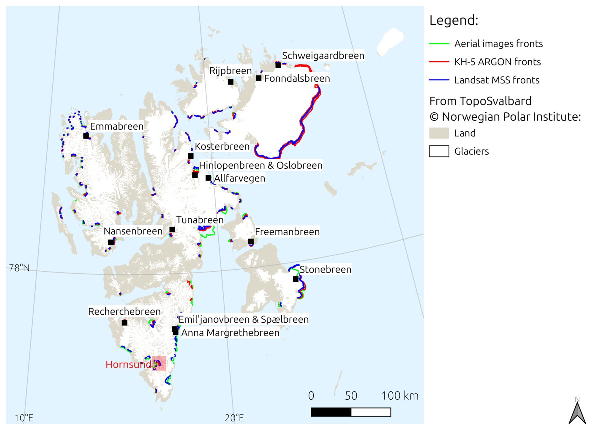
Figure 4 Map of Svalbard displaying the calving fronts contained in our dataset. Placenames mentioned in the text are labeled on the map.

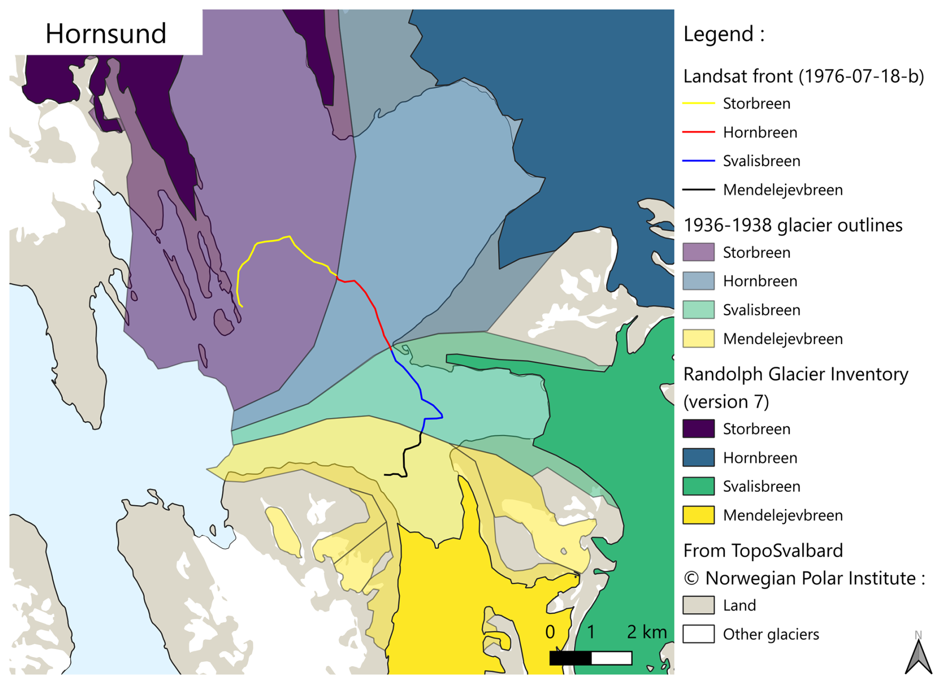
Figure 5 Example of split of glacier fronts in Hornsund (cf. red box in Fig. 4). RGI (RGI 7.0 Consortium, 2023, plain) and 1936 (semi-transparent) outlines are also displayed to show the boundaries between the different glaciers.

2.5 Glacier frontal changes characterization

This study focuses on quantifying glacier frontal changes. Since calving fronts may have a complex geometry and may not move uniformly, we focus on reducing the problem to quantifying their position change along the glacier flow axis. We used the extrapolated centerline method, introduced by Lea et al. (2014), as an improvement of the centerline method. In the regular centerline method, the distance between two front observations is simply calculated as the distance between the intersection of the fronts and the glacier centerline, resulting in a loss of all the information about the front geometry. The extrapolated centerline method uses inverse distance weighting to define the position of every front point on the glacier centerline. The final position of the front is then defined as the mean value of the positions of its points (cf. Lea et al., 2014, for implementation details; the method of this study is identical to theirs). We digitized centerlines by hand, due to the lack of concomitant topography and flow information. We compared the results obtained through this method to those calculated with the box method (Lea et al., 2014) when possible. We found a strong agreement between both methods. Since the extrapolated centerline method is designed to improve tracking of glaciers with changes in front width and non-rectilinear flows (Lea et al., 2014), we chose it to calculate all the results.

We retrieved area change by multiplying glacier front displacements (calculated with the previously presented methods) and the average lengths of the fronts (Li et al., 2025). In this study, we calculated cumulative area change by adding the contributions of all glaciers together.

2.6 Uncertainties

For the fronts that were obtained from KH-5 ARGON and Landsat MSS images, we assessed the positioning uncertainty by comparing fronts that were digitized from images dating from the same year. We consider this method to be reliable as Landsat MSS images were all taken during summer, and KH-5 ARGON images were taken in series on the same day. Therefore, the true position of a front should be the same on two photographs from the same year. Harcourt et al. (2026) identified three marine-terminating glaciers that were possibly in active surge phase when the Landsat images were taken: Allfarvegen (1970–1980), Rijpbreen (1938–1992) and Bodleybreen (1976–1980). We therefore excluded these glaciers from the Landsat uncertainty calculations. The typical positioning uncertainties for each year are summarized in Table 2. We also recombined these values to calculate uncertainties on front displacements and on cumulative area change. Since the qualities of the georeferencing and the front delineation depend mainly on the image quality, we calculated one value for each uncertainty type per year or possible combination of years (cf. Appendix B for calculation details).

Table 2 Positioning uncertainties for each year, calculated from the standard deviations of distributions of distances between fronts dating from the same year (cf. Appendix B1)

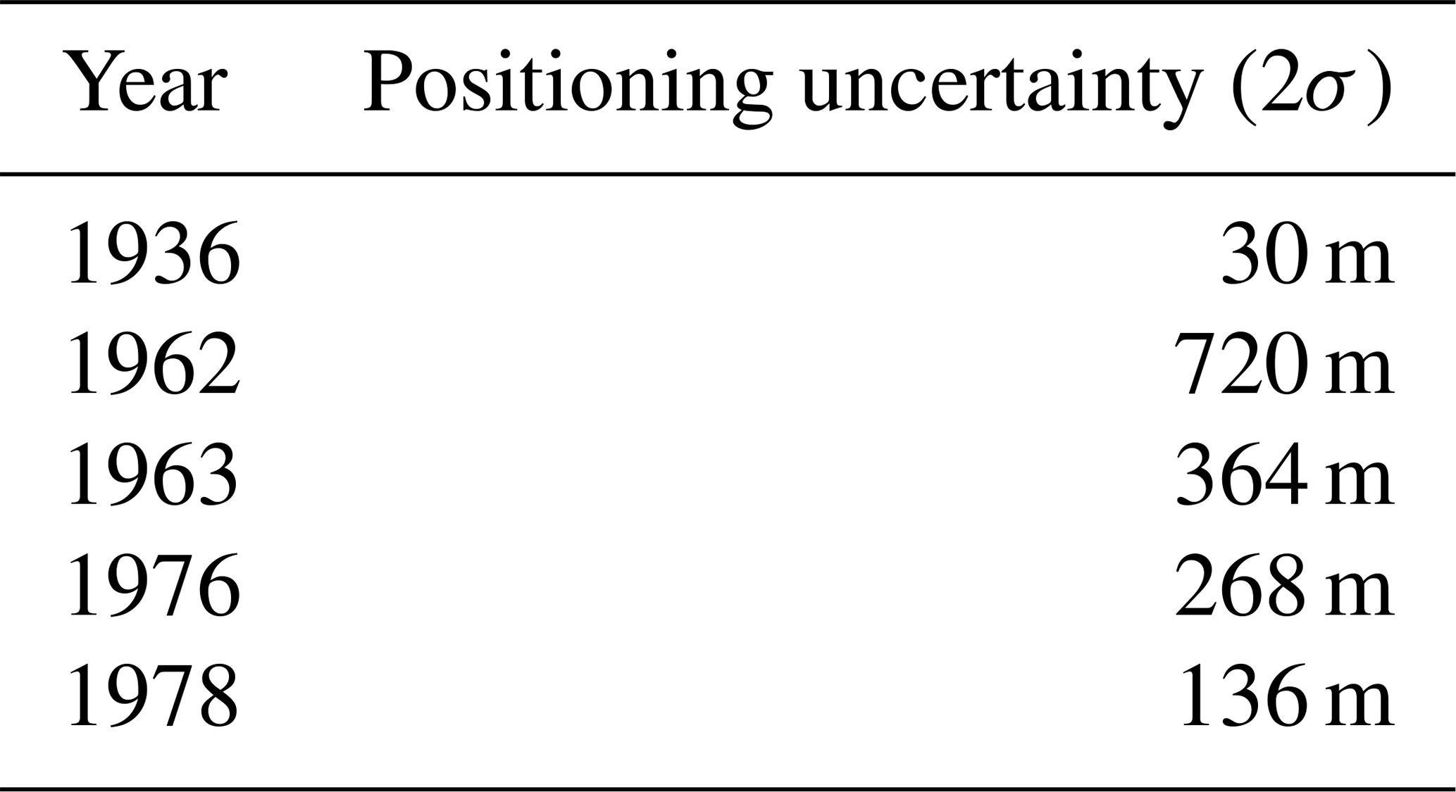
RMSE values calculated for GCP positions are provided in Appendix B2. These RMSE values are high: up to 389 m for KH-5 ARGON (frame 1962-05-16-b) and 200 m for Landsat (frame 1976-07-18-b). However, these values are lower than those we obtained with our uncertainty assessment based on front comparisons (Table 2). Indeed, our uncertainty assessment accounts for georeferencing errors, delineation precision and human mistakes at glacier positions. Therefore, our uncertainties are conservatively bigger than these RMSE values. Moreover, since all fronts were digitized within the bounds of the GCPs, the risk of extensive extrapolation due to polynomial georeferencing transformations is limited. If unidentified systematic biases exist, they are included in our uncertainty assessment.

High positioning uncertainties and RMSE may lead to inaccurate front displacement calculations, which impact both average frontal change assessment and individual advance/retreat identification. To mitigate this risk, we calculated uncertainties on frontal changes (cf. Sect. 3.1) and filtered all retreats/advances that were not in the 95 % interval (cf. Sect. 3.2).

3 Results

3.1 Average frontal change

Figure 6a displays time series of front positions (corrected to set their values to zero in 1936–1938). The mean glacier front position is also shown, as well as its associated uncertainties. Using a weighted least squares (WLS) method, we calculated that Svalbard tidewater glaciers retreated by $\mathrm{27.3}\pm \mathrm{3.0}\mathrm{m}{\mathrm{yr}}^{-\mathrm{1}}$ between 1936–1978. This average glacier linear retreat represents 1140±136 m in 1978, compared to 1936–1938. The graphs show a faster retreat rate between 1936–1938 and 1962–1963, followed by a plateau until 1976–1978. The retreat rate seems to increase again between 1976–1978. However, because of the lack of data points between 1936–1938 and 1962–1963 and the overall high uncertainties (especially in 1962–1963), our observations could also reflect a linear retreat throughout the entire study period. Therefore, differences between 1936–1962 and 1963–1978 are difficult to assess robustly. One can also see the diversity of behaviors of Svalbard tidewater glaciers (gray lines on Fig. 6a): most are retreating, but some are advancing, and they have a wide variety of retreat/advance rates.

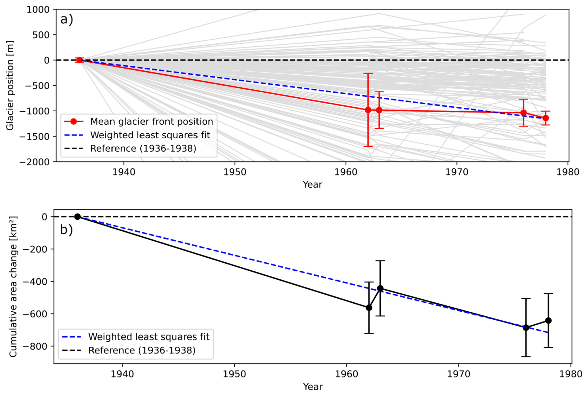
Figure 6 Time series of front positions (a) and cumulative area loss (b). The positions have been corrected so that the origin corresponds to 1936–1938. The gray lines represent individual glacier fronts (a), the red line corresponds to the mean glacier front position (a), and the dashed blue lines to the general trend (a and b). The error bars define the 95 % confidence interval (2σ) based on the corrected standard deviations calculated in Appendix B1 (a) and Appendix B4 (b).

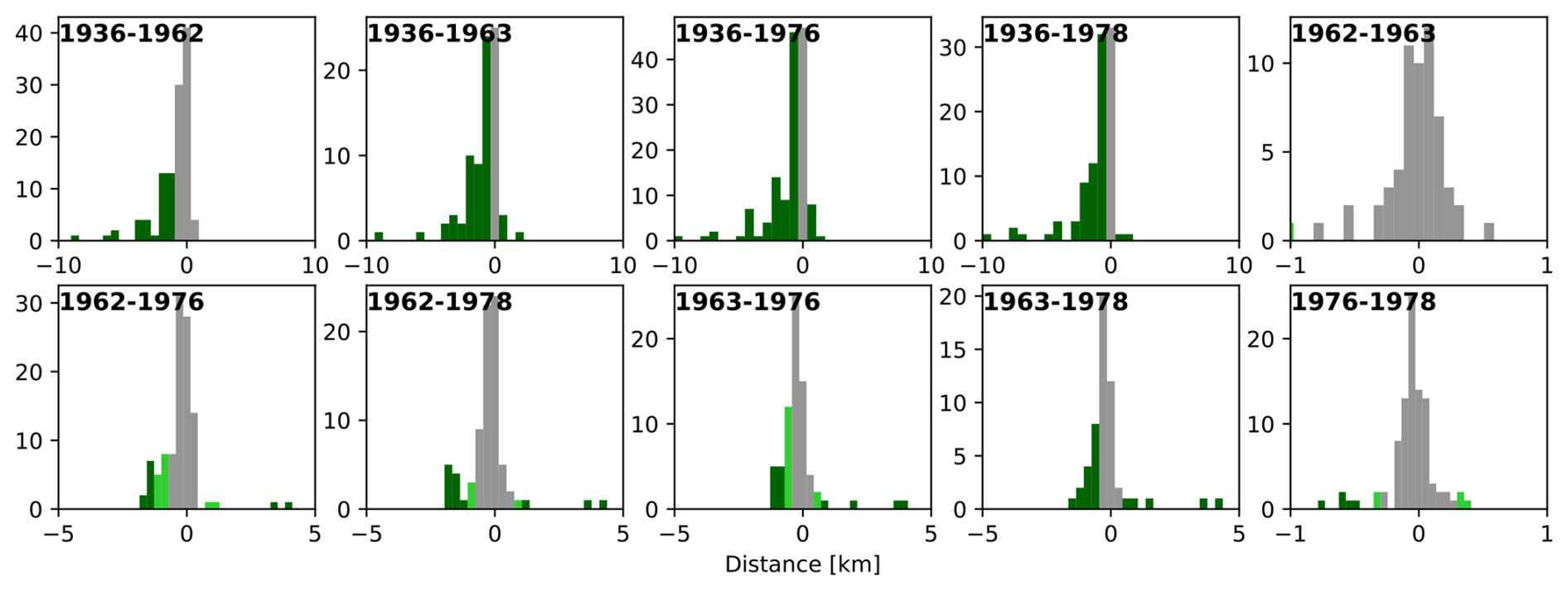
Figure 7 Distributions of distances between two fronts for every possible year combination. Colors represent the degree of confidence with which a retreat or advance of the front was detected: light green – 2σ (95 %); dark green – 3σ (99 %). Uncertainties are based on the recombined variances calculated in Appendix B3.

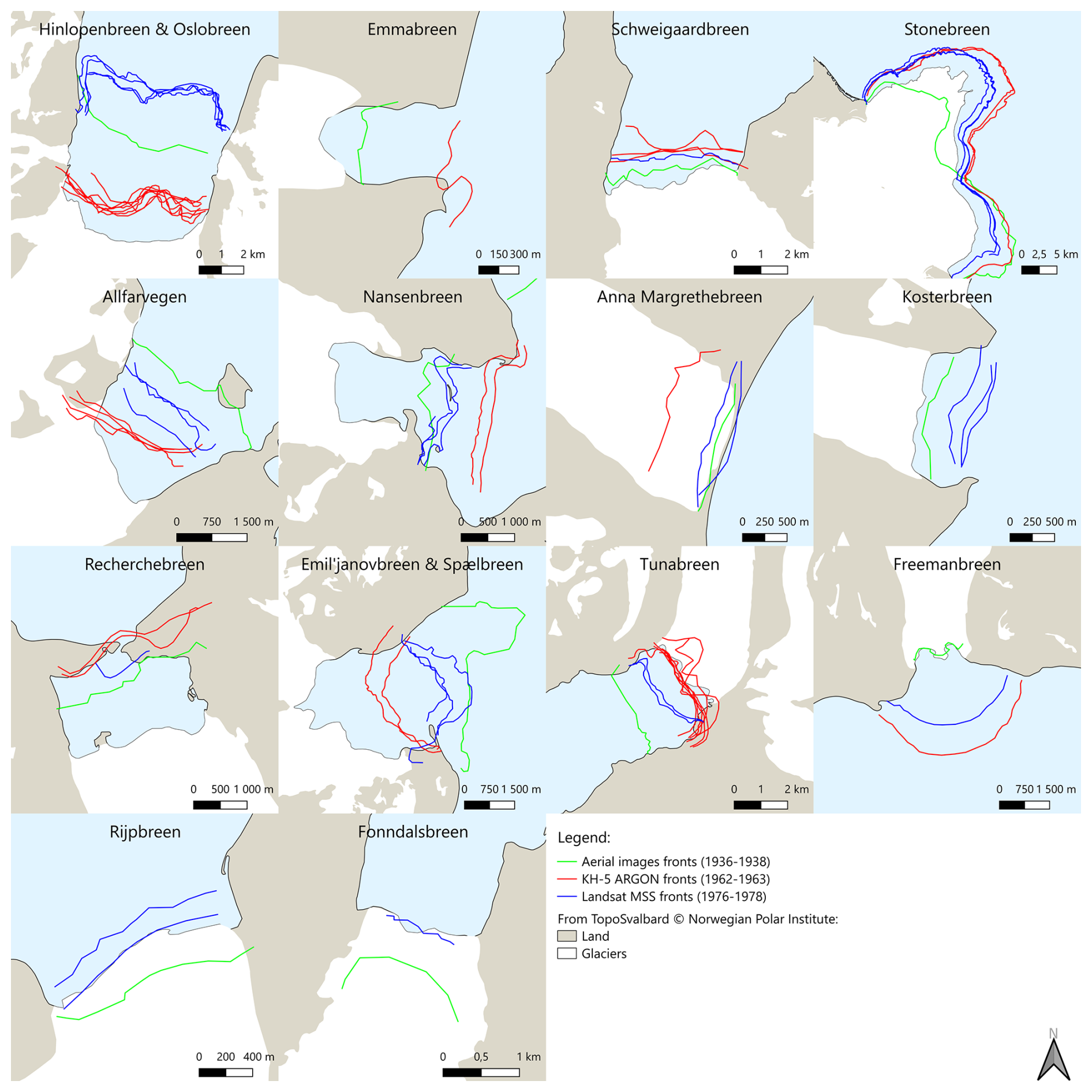
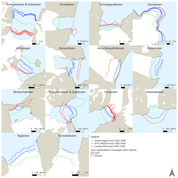
Figure 8 Maps of the main front advance events. Fronts from aerial images (1936–1938) are in green, KH-5 ARGON fronts (1962–1963) are in red and Landsat MSS fronts (1976–1978) are in blue. For the glacier locations in the archipelago, see Fig. 4.

Figure 9 Spatial average of ERA5 T2m (a), SST and SIC (b) over Svalbard between 1940–2023. The blue (resp. gray) area represents the time frame covered by this study (resp. Li et al., 2025).

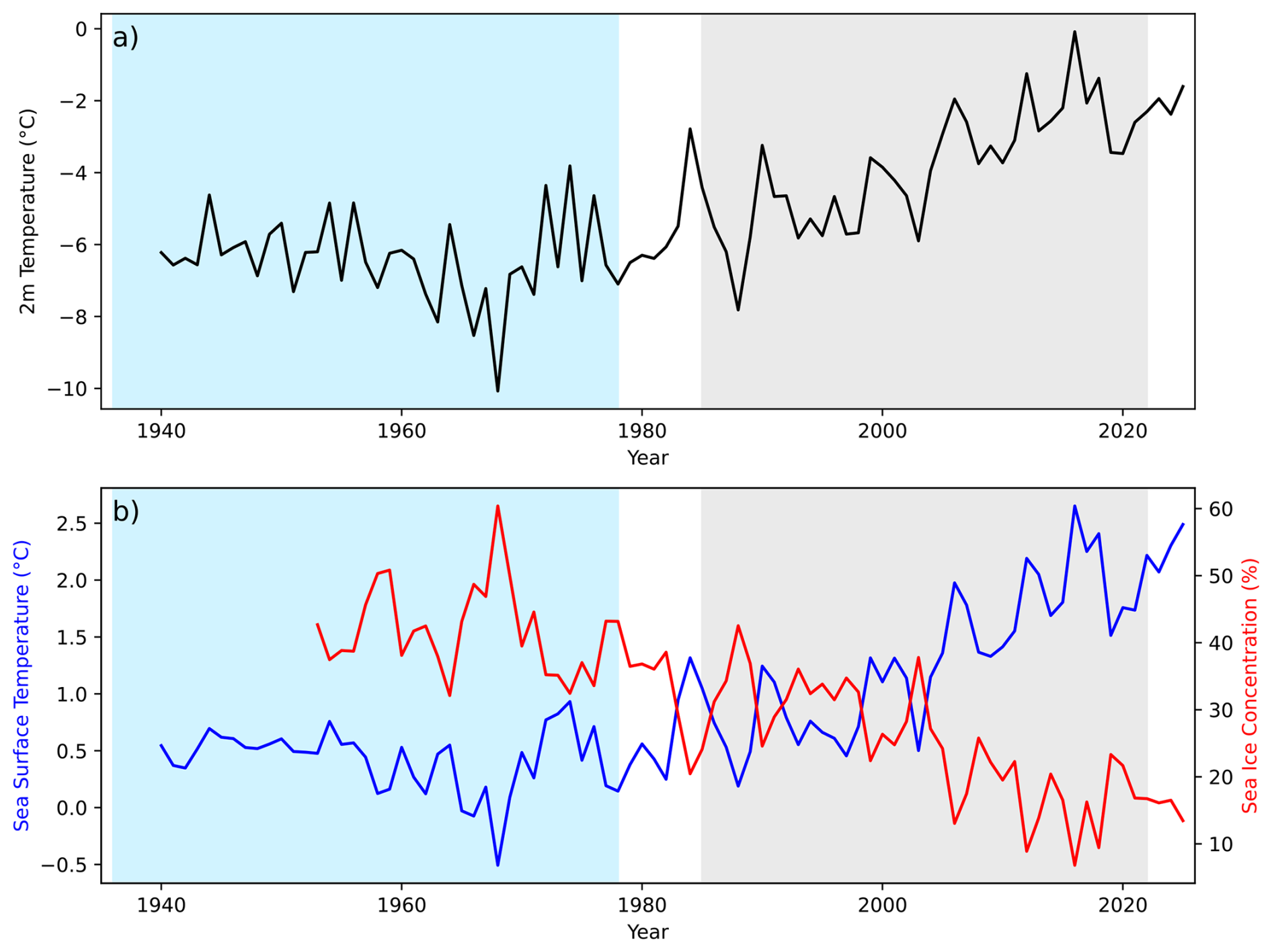
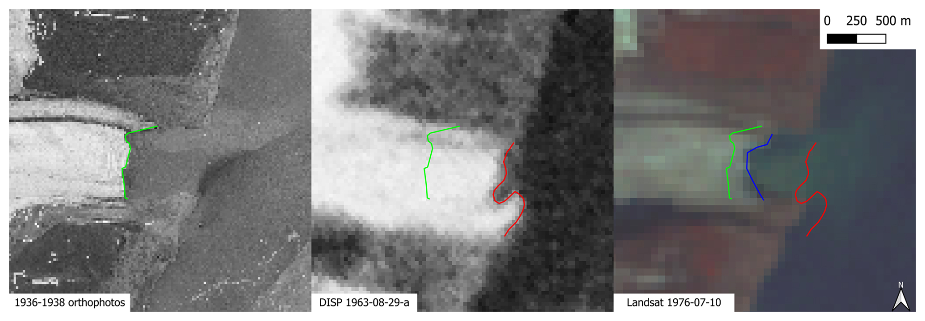
Figure 10 1936–1938 aerial photograph (left), 1963 DISP (center) and 1976 Landsat MSS (right) images for the Emmabreen surge. The green line (resp. red, blue) corresponds to the 1936–1938 (resp. 1963, 1976) front. Image credits: Norwegian Polar Institute (aerial image) and U.S. Geological Survey (DISP and Landsat).

Table 3 Advance events detected, and corresponding documented glacier surges. The letters correspond to the references: Liestøl (1969) (LI), Lefauconnier and Hagen (1991) (LE), Hagen et al. (1993) (HA), and Błaszczyk et al. (2009) (BL). Glaciers in bold indicate the events for which additional information has been provided in this study.

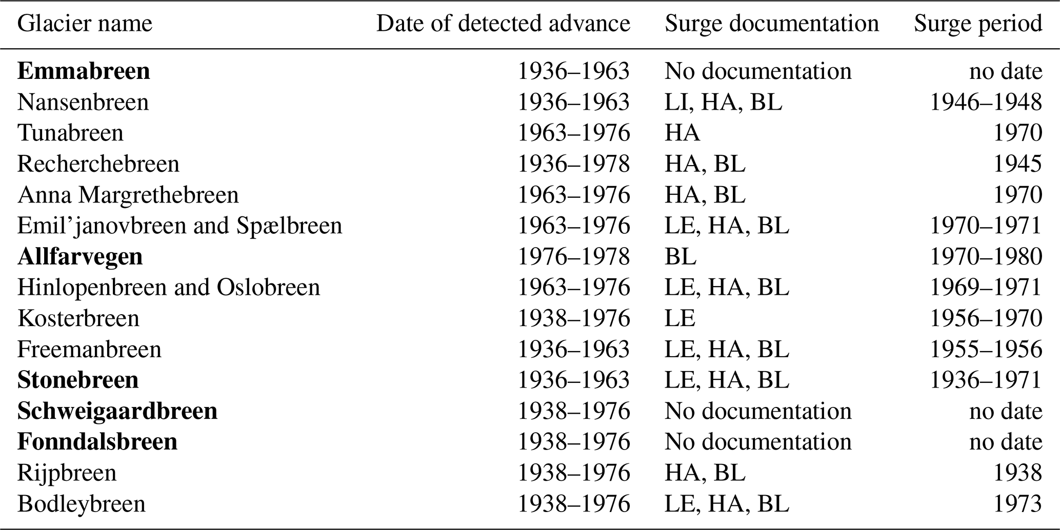
Figure 6b shows the cumulative area change due to calving front displacements for all measured glaciers between 1936–1978. The area loss between 1936–1978 was 642±167 km², with an average area loss rate of $\mathrm{17.0}\pm \mathrm{2.5}{\mathrm{km}}^{\mathrm{2}}{\mathrm{yr}}^{-\mathrm{1}}$.

3.2 Individual glacier events

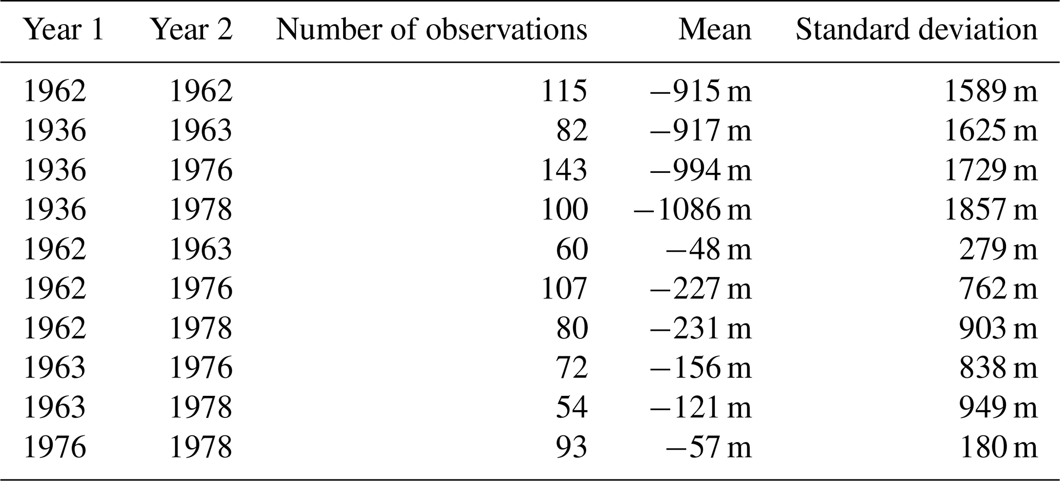
To identify significant retreat and advance events, we compared all front observations together, for each glacier. Then, we identified pairs of fronts whose distances were higher than the recombined uncertainties presented in Appendix B3. These events correspond to front advances or retreats with at least a 95 % confidence. Figure 7 shows the distance distributions and highlights the significant events. Table C1 in the Appendix summarizes the number of observations used for each distribution, and shows their mean values and standard deviations. Several observations can be made about these distributions. First, the mean values are all negative, meaning that on average, the fronts are observed to retreat. Second, dispersions are higher when the time span between front observations is greater. Finally, more significant observations are made when the uncertainties on front positions for both years are low, and when the time span between the observations is long.

We identify a total of 15 advances and 122 retreats between 1936–1978. A 16th advance of Storisstraumen was detected between 1976–1978, but this is likely due to the georeferencing uncertainty of the Landsat images. The uncertainty is high in this region due to the lack of stable terrain to be used as georeference points. Therefore, this glacier has been removed from the results. On Fig. 8, maps for all filtered advance events are displayed. One can observe on these maps that a specific front can show both advance and retreat behaviors. For instance, Hilopenbreen retreated between 1938 and 1962–1963 and then advanced between 1962–1963 and 1976–1978, and Freemanbreen advanced between 1936–1963 and then retreated between 1963–1976. Also, an advance/retreat might not be uniform along the front (e.g. Stonebreen), which we bring up further in the discussion.

Because of the high uncertainties (especially in 1962–1963), it is necessary to calculate the distance between fronts for every possible pair of years, and not only between consecutive observations. For example, a visual inspection of the Recherchebreen's fronts (Fig. 8) supports an advance of the front between 1936–1962. However, the uncertainties on the 1962 delineations are much higher compared to those of 1978. Therefore, the distance between the 1936 and 1962 fronts is not significant to conclude to an advance, whereas the distance between the 1936 and 1978 fronts is lower but significant when compared to the displacement uncertainty. Thus, the advance is only detected between 1936–1978.

4 Discussion

4.1 Average frontal change

We calculated an average retreat rate of $\mathrm{27.3}\pm \mathrm{3.0}\mathrm{m}{\mathrm{yr}}^{-\mathrm{1}}$ for the 171 tracked glaciers between 1936–1978. Li et al. (2025) found a wide variety of front change rates for 1985–2023, although most are within the range of 25–50 m yr⁻¹, which is of the same order of magnitude as the one we calculated for a prior time frame. We found a cumulative area loss rate of $\mathrm{17.0}\pm \mathrm{2.5}{\mathrm{km}}^{\mathrm{2}}{\mathrm{yr}}^{-\mathrm{1}}$ for all the tracked glaciers between 1936–1978, which is consistent, though lower, compared to the value of 23.78 km² yr⁻¹ calculated by Li et al. (2025) for the 1985–2023 period, and the value of $\mathrm{26.79}\pm \mathrm{0.54}{\mathrm{km}}^{\mathrm{2}}{\mathrm{yr}}^{-\mathrm{1}}$ calculated by Kochtitzky and Copland (2022) for 2000–2020. This could indicate an acceleration of the area loss of Svalbard marine-terminating glaciers due to calving front retreats over the past century.

Figure 9 displays the time series of 2-meter temperature (T2m), sea surface temperature (SST) and sea ice concentration (SIC) from the ERA5 reanalysis (Copernicus Climate Change Service, 2019), yearly averaged over Svalbard (74–81° N, 7–35° E) between 1940–2023. The graph clearly shows an overall increase in T2m and SST, and a decrease in SIC over the whole period. In fact, the average T2m is −6.42 °C for 1940–1978 and −4.05 °C for 1979–2023, the average SST is 0.42 °C for 1940–1978 and 1.23 °C for 1979–2023, and the SIC is 41.93 % for 1953–1978 (no SIC data is available prior to 1953) and 25.58 % for 1979–2023. Therefore, the evolutions of all three variables support an acceleration of the calving fronts' retreat after 1978 (Luckman et al., 2015; Otero et al., 2017; Błaszczyk et al., 2023) and are consistent with our results.

However, several differences in the methods to calculate these numbers remain: like Li et al. (2025), we calculate the change in area as the product of the retreat length and the glacier width, but we keep surge-type glaciers in the dataset for this calculation, and do not take into account the seasonal variability. The number given by Kochtitzky and Copland (2022) includes Svalbard and Jan Mayen, and surge-type glaciers are kept in this dataset. However, they manually digitized the outline of the area that changed from glacier-covered to not glacier-covered, instead of calculating it as a product of retreats' lengths and glacier's widths. Li et al. (2025) assessed the possible error sources arising from the comparison of their results with those of Kochtitzky and Copland (2022). They concluded that it remained valid to assess a large scale trend rather than to give a precise estimate. This discussion being limited to the former, we believe the comparison remains valid.

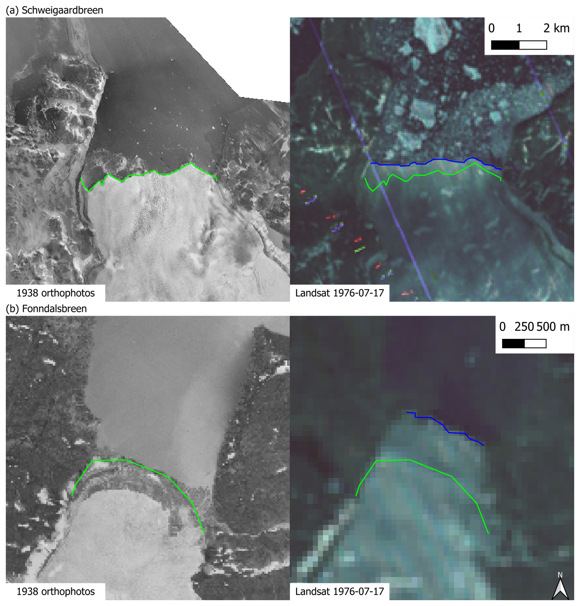
Figure 11 1938 aerial photograph (left) and 1976 Landsat MSS (right) images for the Schweigaardbreen (a) and Fonndalsbreen (b) advances. The green lines (resp. blue) correspond to the 1938 (resp. 1976) fronts. Note the different scales for the two glaciers. Image credits: Norwegian Polar Institute (aerial images) and U.S. Geological Survey (Landsat).

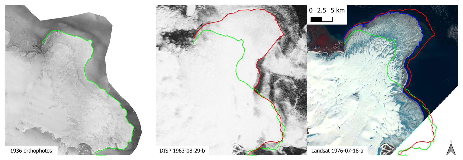
Figure 12 1936 aerial photograph (left), DISP (center) and Landsat MSS (right) images for the Stonebreen surge. The green line (resp. red, blue) corresponds to the 1936 (resp. 1963, 1976) front. Image credits: Norwegian Polar Institute (aerial image) and U.S. Geological Survey (DISP and Landsat).

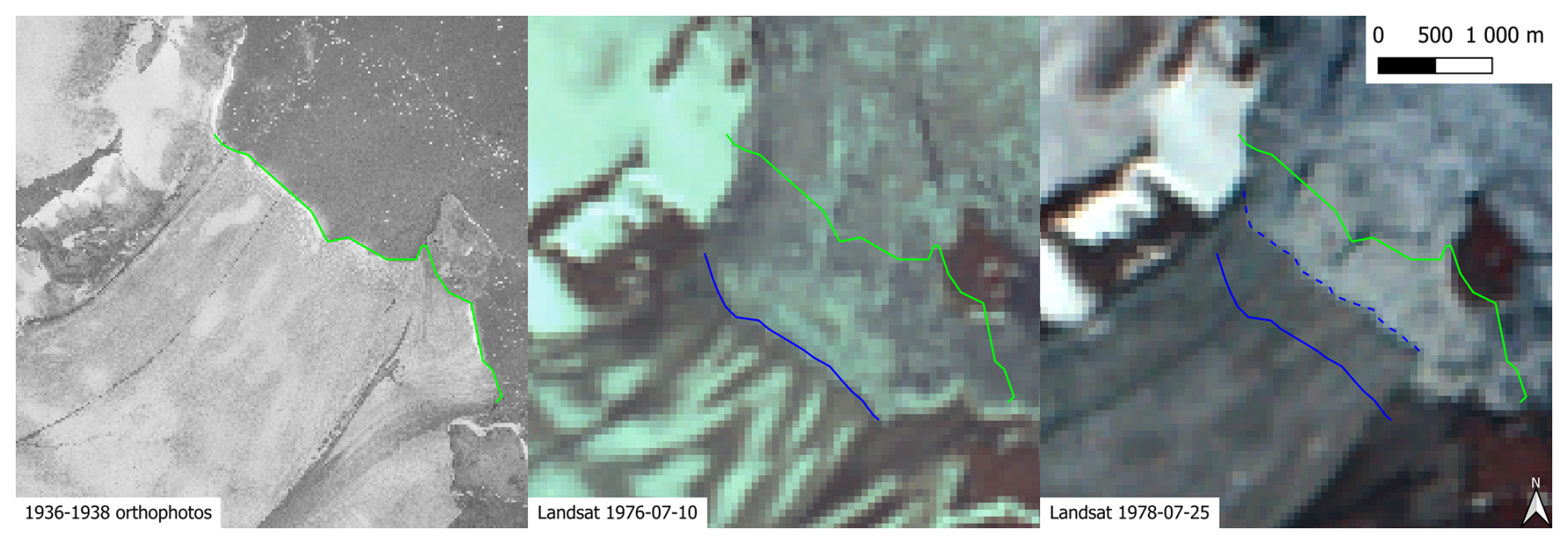
Figure 13 1938 aerial photograph (left), 1976 (center) and 1978 Landsat MSS (right) images for the Allfarvegen surge. The green line (resp. blue, dashed blue) corresponds to the 1938 (resp. 1976, 1978) front. Image credits: Norwegian Polar Institute (aerial image) and U.S. Geological Survey (DISP and Landsat).

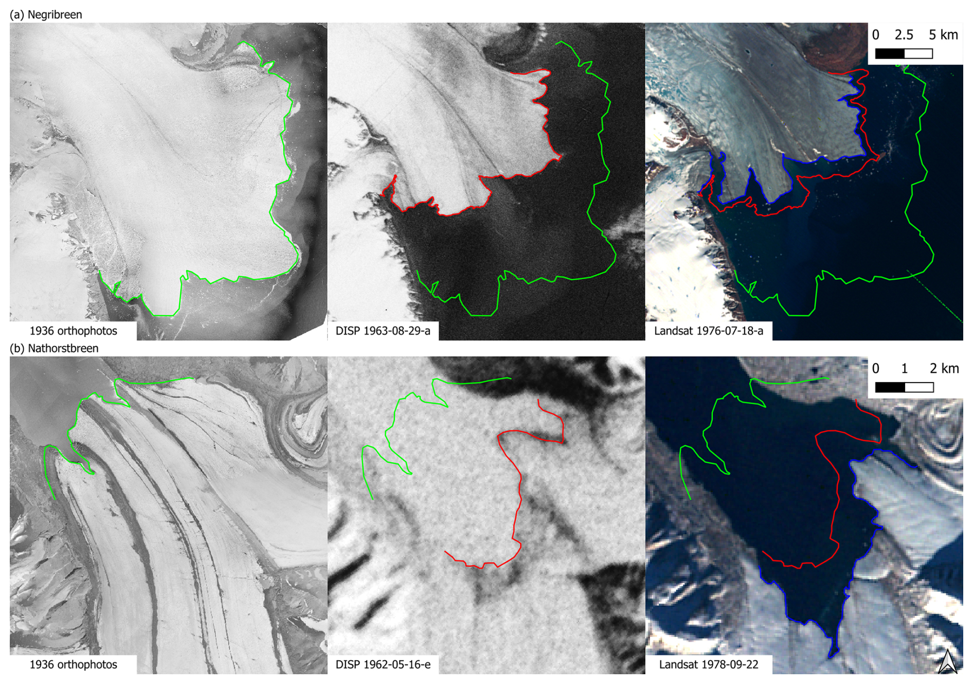
Figure 14 1936 aerial photograph (left), 1962–1963 DISP (center) and 1976–1978 Landsat MSS (right) images for the Negribreen (a) and Nathorstbreen (b) retreats. The green lines (resp. red, blue) correspond to the 1936 (resp. 1962–1963, 1976–1978) fronts. Note the different scales for different glaciers. Image credits: Norwegian Polar Institute (aerial images) and U.S. Geological Survey (DISP and Landsat).

4.2 Individual glacier events

We detected a total of 13 glacier surges and 2 other advances (cf. Sect. 4.2.2). Table 3 lists all the surge/advance events we detected, and reports the studies that mention them, as well as the time windows they identified. For two glaciers (Allfarvegen and Stonebreen, cf. Sect. 4.2.3), we narrowed the time window in which the surge was known to happen, and we discovered one new undocumented surge of Emmabreen (cf. Sect. 4.2.1).

4.2.1 Surge of Emmabreen between 1936–1963

The Emmabreen surge appears clearly on Figs. 8 and 10: in 1963, the glacier front reaches the bay mouth, whereas in the 1936 aerial and 1976 Landsat images, the front lies further into the bay. The front advanced by 450 m between 1936–1968. Two fronts from 1963 are available in the dataset, about 500 m away from each other. However, the front that was digitized from the 1963-09-29-b image was on the edge of the photograph, where the deformations for this specific image (cf. Sects. 2.2.2 and B2) are stronger and the georeferencing less accurate. We did not take this front into account in the calculations as it does not intersect the centerline for this glacier, and therefore did not display it on Fig. 8.

Geyman et al. (2022) calculated a negative geodetic mass balance of $\mathrm{0.24}\pm \mathrm{0.07}\mathrm{m}\mathrm{w}.\mathrm{e}.{\mathrm{a}}^{-\mathrm{1}}$ for Emmabreen for 1936–2010. Therefore, the observed advance is extremely difficult to explain by other means than a surge. RGI 7.0 Consortium (2023) did not classify Emmabreen as a surge-type glacier, but Harcourt et al. (2026) reported a surge between 2011–2021. We therefore conclude that Emmabreen has surged twice in the last century; between 1936–1963, and in the 2010s.

4.2.2 Advances of Schweigaardbreen and Fonndalsbreen

Schweigaardbreen is not documented as a surge-type glacier, but the presence of a glaciotectonic composite ridge system seen in recent aerial images (Lovell and Boston, 2017) indicates a possible misclassification. The images shown in Fig. 11a show an advance of about 400 m between 1938–1976. Therefore, we conclude that our observations are compatible with a possible surge of Schweigaardbreen. The 1962 DISP images are too inaccurate to narrow down the time frame of the advance. Similarly, we registered a 541 m advance of the neighboring Fonndalsbreen between the same years (Fig. 11b). Geyman et al. (2022) calculated a positive geodetic mass balance of $\mathrm{0.07}\pm \mathrm{0.18}\mathrm{m}\mathrm{w}.\mathrm{e}.{\mathrm{a}}^{-\mathrm{1}}$ for Fonndalsbreen between 1936–2010. Schweigaardbreen is not included in this dataset but we assume very similar conditions to Fonndalsbreen, given its proximity (about 50 km on the same ice cap) and similarity in recent elevation change rates (Moholdt et al., 2010). Therefore, advances of these two glaciers may have been entirely mass-balance driven, and we refrain from categorizing them as surges and report them as advances instead.

4.2.3 Narrowing the timeframes of the surges of Stonebreen and Allfarvegen

An advance of 1664 m of the northern tongue of Stonebreen between 1936–1963 can be observed in Figs. 8 and 12. This surge was already documented by Lefauconnier and Hagen (1991), Hagen et al. (1993), and Błaszczyk et al. (2009), and its known time frame was 1936–1971. Our observations narrow down this time frame to 1936–1963.

A complicating factor for this event when comparing it with a modern surge that just recently terminated (Mannerfelt et al., 2025) is that the two surges occurred in two different parts of the ice body. This is important for studies focused on “return times” of glacier surges; the Stonebreen surge has not necessarily reoccurred but instead started in a new unique location. In other words, our study shows that the two surges of Stonebreen are only related through the naming convention of the ice cap.

Finally, we observe an advance of 380 m of Allfarvegen between 1976–1978. A surge of this glacier in the 1970s was documented by Błaszczyk et al. (2009). Our observations narrow down this time frame to 1976–1978.

4.2.4 Retreats of Negribreen and Nathorstbreen 1938–1978

Among the 122 significant retreats detected, Negribreen's and Nathorstbreen's ones are the two most significant, with values of about 7300 and 7600 m, respectively. Figure 14 shows the satellite and aerial images corresponding to these events. An important surge of Negribreen is known during 1935–1936 (Lefauconnier and Hagen, 1991; Hagen et al., 1993). Nathorstbreen surged in 1890, as well as Liestølbreen and Doktorbreen – two neighboring glaciers whose fronts merge with Nathorstbreen's one – surged between 1870–1880 (Harcourt et al., 2026).

4.3 Use of archived satellite images

In this study, we used archived satellite imagery to determine glacier calving front positions on Svalbard. However, it is likely that the dataset also contains geophysical information that is outside the scope of our study. A natural example of such information is the extent of land-terminating glaciers. It is possible that the images show previously undocumented surges of land-terminating glaciers, or at least can be used to better constrain the times of past surges in the same manner as we have done in our study for marine terminating ones. To facilitate future research, we have made all the data available, including the georeferenced satellite images. Furthermore, this study has shown that the KH-5 ARGON images are useful for the study of the Svalbard glaciers. Thus, we suggest that their use for other remote geographic areas be explored.

5 Conclusions

In this study, we have used three different types of aerial and satellite images to investigate historical changes in Svalbard tidewater glacier fronts between 1936–1978. We have successfully obtained calving fronts from Landsat MSS multispectral images and DISP, and compared our observations to the glacier outlines from 1936–1938 to assess the retreat or advance of the glaciers. To the best of our knowledge, this is the first study to use DISP over Svalbard.

An analysis of the average glacier behavior between 1936–1978 yields an average retreat rate of $\mathrm{27.3}\pm \mathrm{3.0}\mathrm{m}{\mathrm{yr}}^{-\mathrm{1}}$, which agrees with the value of 25–50 m yr⁻¹ found by Li et al. (2025) for 1985–2023. We calculated a cumulative area loss rate of $\mathrm{17.0}\pm \mathrm{2.5}{\mathrm{km}}^{\mathrm{2}}{\mathrm{yr}}^{-\mathrm{1}}$. This loss is of the same order of magnitude, though slightly lower than the value of 23.78 km² yr⁻¹ calculated by Li et al. (2025) for 1985–2023 and that of $\mathrm{26.79}\pm \mathrm{0.54}{\mathrm{km}}^{\mathrm{2}}{\mathrm{yr}}^{-\mathrm{1}}$ found by Kochtitzky and Copland (2022) for 2000–2020. It is likely due to increasing T2m and SST in Svalbard, as well as a decrease in SIC between 1940–2023. Finally, we conducted an extensive comparison of all the fronts and identified 13 glacier surges. For four of these glaciers, our study brings new information: we discovered an undocumented surge of Emmabreen (1936–1963) and narrowed down the time frames of two known surges: Allfarvegen (1976–1978) and Stonebreen (1936–1963). We also documented an advance of Schweigaardbreen and Fonndalsbreen between 1938–1976.

To continue this study, future work should focus on improving the precision of the observations, especially for those obtained from DISP. This can be done by orthorectifying the images, but may require access to calibration data. The analysis could be extended as well, by assessing the spatial variability of the average retreat rate. The dataset containing all the calving fronts is freely available.

Appendix A: Full names of the satellite images

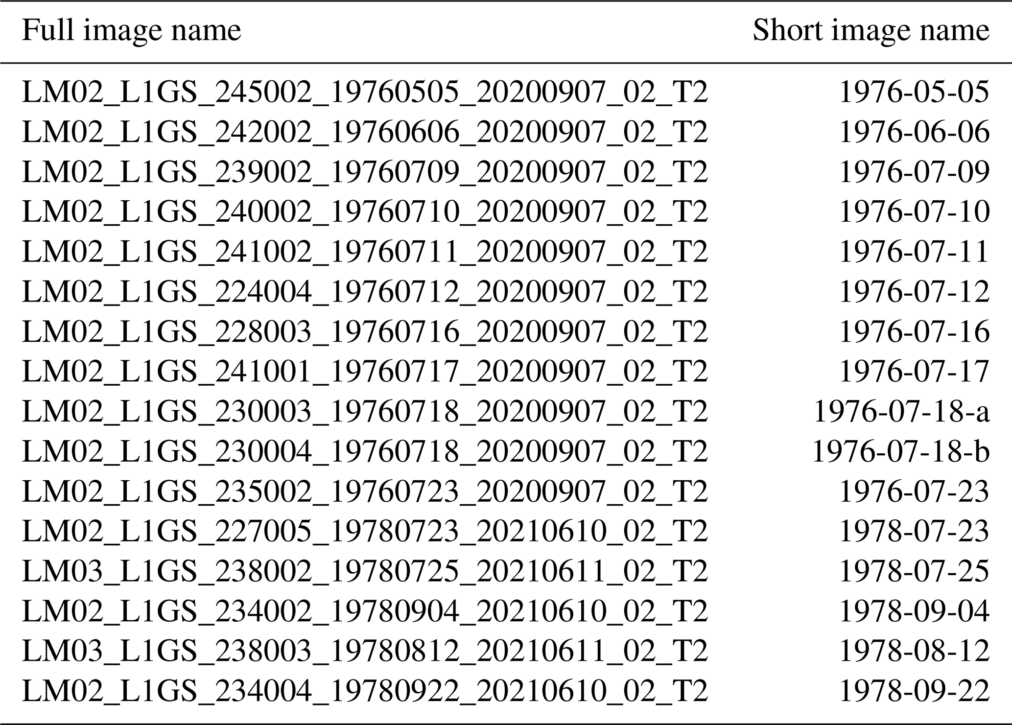
To facilitate the reading of this paper, we have shortened the names of the satellite images. Table A2 (resp. Table A1) provides the full names of all the used Landsat MSS (resp. KH-5 ARGON) images. These names are the ones used in the EarthExplorer platform.

Table A1 Full names of the KH-5 ARGON images used in this study (U.S. Geological Survey, 2021).

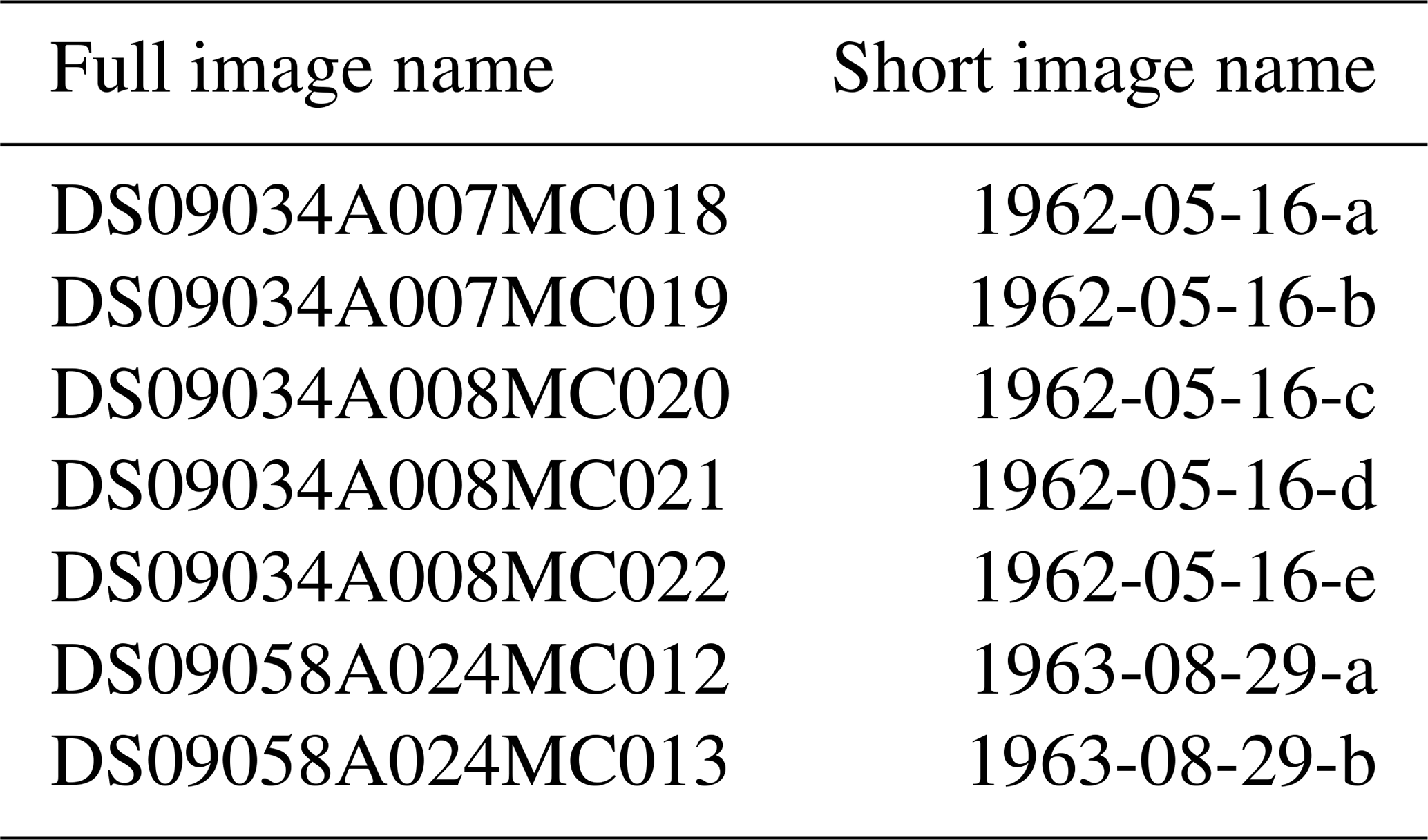
Table A2 Full names of the Landsat MSS images used in this study (U.S. Geological Survey, 2020b).

Appendix B: Details of uncertainty calculations

B1 Front positions

Figure B1 displays the distributions of distances calculated between fronts dating from the same year. For KH-5 ARGON images, one can observe that more observations were available for the year 1962 (five images in 1962, only two in 1963). One can also see that distances are more dispersed in 1962. This is maybe due to the greater number of available observations, but more certainly to the sea ice conditions at the time of capture: in May 1962, a lot of sea ice was present in the fjords, and therefore glacier fronts were more difficult to distinguish. For Landsat MSS images, more observations were available in 1976. Due to the overall higher quality of the images compared to KH-5 ARGON, the distribution is less dispersed. Sea ice conditions were similar on pictures from both years, and false color composites made glaciers easier to distinguish from the background.

These series seem to follow centered normal distributions. The standard deviations (noted σ^′) are indicated on Fig. B1 for each distribution. These standard deviations are calculated for distances between two fronts, which equally contribute to the uncertainty. Therefore, they must be divided by $\sqrt{\mathrm{2}}$ to obtain the standard deviations on front positions. The corrected standard deviations (noted σ) are indicated as well on Fig. B1.

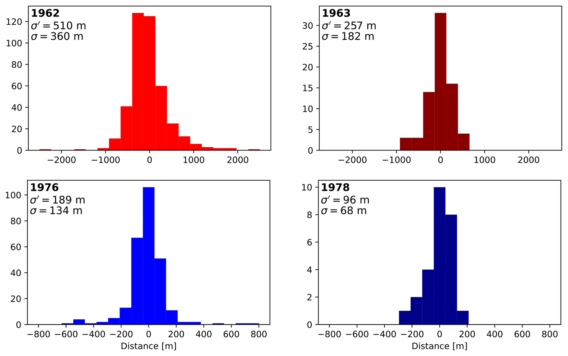
Figure B1 Distance histograms between fronts delineated from KH-5 ARGON (red) and Landsat MSS (blue), ordered by year. The distances were calculated with the extrapolated centerline method. The standard deviations (σ^′), as well as the corrected standard deviations on front positions ($\mathit{\sigma }=\frac{{\mathit{\sigma }}^{\prime }}{\sqrt{\mathrm{2}}}$) are indicated in the top-left corner of each plot.

For the 1936–1938 fronts, the uncertainty on glacier outlines was already assessed by Geyman et al. (2022), and its value is 30 m.

B2 RMSE on GCP positions

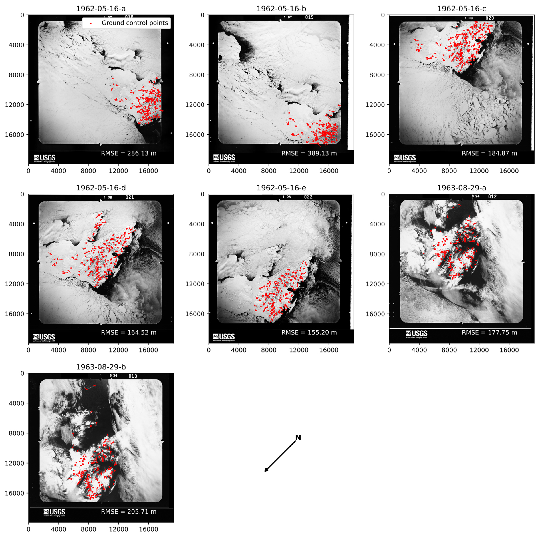
Figure B2 KH-5 ARGON images, GCPs and residuals, expressed in pixel coordinates. The residuals have been multiplied by 50 to enhance readability. The RMSEs are given in the bottom-right corner of each subplot, and the black arrow on the last row indicates the approximate north direction. Image credits: U.S. Geological Survey.

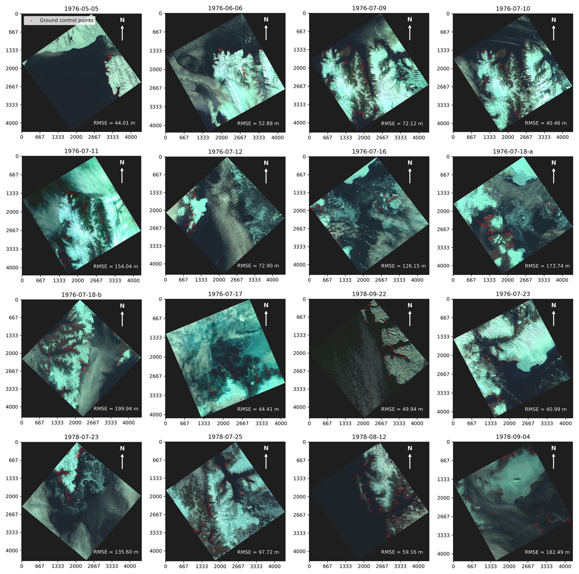
Figure B3 Landsat images, GCPs and residuals, expressed in pixel coordinates. The residuals have been multiplied by 50 to enhance readability, and the RMSEs are given in the bottom-right corner of each subplot. Image credits: U.S. Geological Survey.

Figures B2 and B3 display the spatial distributions of residuals calculated on the GCPs for DISP and Landsat images, as well as RMSEs. One can observe there is no clear similar pattern between the images. Overall, RMSEs on DISP are comparable or higher to the typical geometric accuracies (140–200 m) obtained for this type of images after orthocorrection (see Table 5 in Ye et al., 2017).

For DISP, frame 1962-05-16-b presents the highest RMSE, which is probably due to all the GCPs being located in the corner of the image. This is consistent with a higher positioning uncertainty for year 1962. For Landsat, frame 1978-09-04 is the only one with a higher RMSE than the calculated uncertainty. Only 25 fronts (out of 467 for Landsat) were obtained from this image; the impact on the average frontal change results is therefore negligible. Moreover, none of the individual advance/retreat observations at year 1978 rely solely on one of these observations.

B3 Front displacements

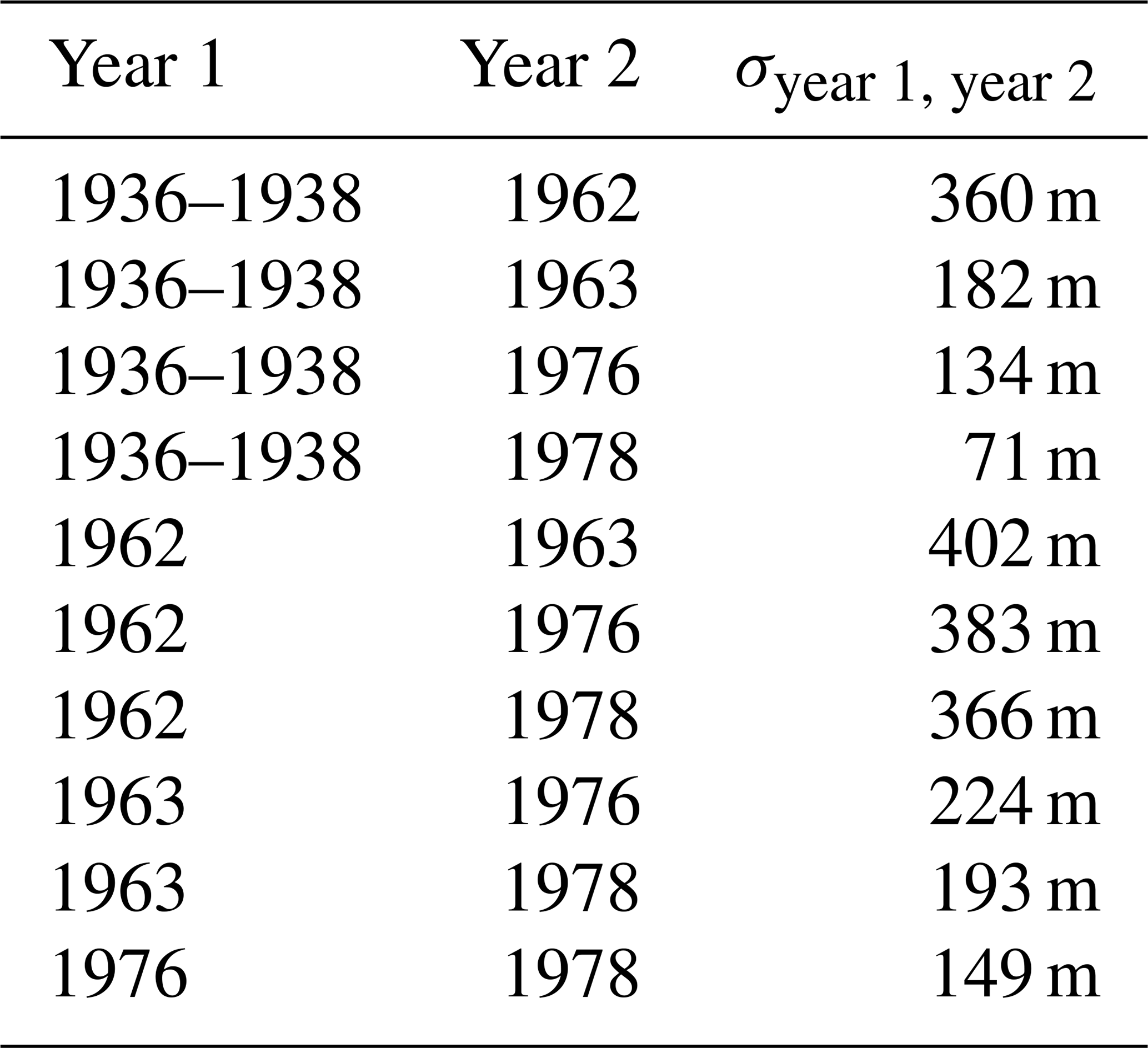
The standard deviations on front positions can be recombined to assess the uncertainty on the distance calculated between the measures of two different years. Indeed, if σ_{year 1} and σ_{year 2} are the position uncertainties for two different years, then the uncertainty on front displacement σ_{year 1, year 2} between these two years is:

$${\mathit{\sigma }}_{\text{year 1, year 2}}=\sqrt{{\mathit{\sigma }}_{\text{year 1}}^{\mathrm{2}}+{\mathit{\sigma }}_{\text{year 2}}^{\mathrm{2}}}$$

All the possible standard deviations are summarized in Table B1.

Table B1 Standard deviations for front distances, measured with extrapolated centerline method.

B4 Area change

Uncertainties on cumulative area change can be calculated using the uncertainties on front positions (σ, Fig. B1) and the standard deviation on front widths.

Let A_ij be a random variable representing the area change for front i between years j and j+1. By definition, A_ij=W_ijD_ij, where W_ij is the width of front i for year j, and D_ij is the displacement of the front i between years j and j+1.

Thus, the cumulative area loss for all glaciers at year k is:

$$\begin{array}{ll}{\displaystyle }{A}_k& {\displaystyle }=\sum _{j=\mathrm{1}}^k\sum _i{A}_{ij}\\ {\displaystyle }& {\displaystyle }=\sum _{j=\mathrm{1}}^k\sum _i{W}_{ij}{D}_{ij}.\end{array}$$

Therefore,

$$\begin{array}{ll}{\displaystyle }& {\displaystyle }{\mathit{\epsilon }}_k^{\mathrm{2}}:=\text{Var}\left(A_k\right)=\text{Var}\left(\sum _{j=\mathrm{1}}^k\sum _i{A}_{ij}\right)\\ {\displaystyle }& {\displaystyle }=\sum _{j=\mathrm{1}}^k\sum _i\text{Var}\left(A_{ij}\right)\\ {\displaystyle }& {\displaystyle }=\sum _{j=\mathrm{1}}^k\sum _i\text{Var}\left(W_{ij}{D}_{ij}\right)\\ {\displaystyle }& {\displaystyle }=\sum _{j=\mathrm{1}}^k\sum _i\left(\text{Var}\left(D_{ij}\right)\mathbb{E}\left(W_{ij}^{\mathrm{2}}\right)+\text{Var}\left(W_{ij}\right)\mathbb{E}(D_{ij}{)}^{\mathrm{2}}\right)\\ {\displaystyle }& {\displaystyle }=\sum _{j=\mathrm{1}}^k\sum _i\left({\mathit{\sigma }}_{j,j+\mathrm{1}}^{\mathrm{2}}\mathbb{E}\left(W_{ij}^{\mathrm{2}}\right)+\text{Var}\left(W_{ij}\right)\mathbb{E}(D_{ij}{)}^{\mathrm{2}}\right)\end{array}$$

Where:

• ε_k is the standard deviation on cumulative area change for year k,

• ${\mathit{\sigma }}_{j,j+\mathrm{1}}$ is the standard deviation on front displacements between year j and years j+1,

• $\mathbb{E}\left(W_{ij}^{\mathrm{2}}\right)$ is average squared width of front i for year j,

• Var(W_ij) is the variance of front i width for year j, and

• 𝔼(D_ij) is the average front i displacement between years j and j+1.

This calculation is equivalent to a sum of relative uncertainties. The error bars on Fig. 6 correspond to the 95 % confidence interval (2ε_k).

Appendix C: Details on distance distributions

Table C1 provides more details on the distances distributions shown on Fig. 7.

Table C1 Number of observations, mean value, and standard deviation for each distribution shown in Fig. 7.