Evolution of Maud Rise Polynya during the last 250 years – a multiproxy ice core reconstruction from coastal Dronning Maud Land, Antarctica

Open ocean polynyas drive deep ocean convection, influencing regional carbon and heat budgets, which in turn influence the ocean circulation and overall climate of Antarctica. The Maud Rise Polynya (MRP), also known as the Weddell Polynya, is one such polynya that forms in the Southern Ocean during early spring or winter months. The extensively studied MRP opening, which occurred during 2016–2017 and 1974–1976, triggered intense convection, ventilating heat from the deep ocean and modifying water mass properties. However, polynya evolution before the satellite era remains poorly understood. Here, we develop a polynya index using multiple proxy records from an ice core in coastal Dronning Maud Land, East Antarctica. Our approach, integrating records of snow accumulation, δ¹⁸O, deuterium excess and ssNa flux, enhances polynya reconstruction, thereby overcoming the limitations of single-proxy methods. The index replicates the 1974–1976 polynya and extends the record to 1774, revealing three major events comparable to the 1974–1976 great polynya event, in the past 250 years, totalling twenty five polynya years (likelihood>0.6). We identified distinct clusters of polynya activity, possibly corresponding to a specific combination of atmospheric circulation patterns and oceanographic preconditioning for MRP development. This study offers a long-term perspective on MRP variability, providing insights into its drivers and climate-related impacts.

1 Introduction

Open ocean polynyas represent one of the most dynamic and influential features in the Southern Ocean system, serving as critical regulators of heat and gas exchange between the ocean and atmosphere. These persistent areas of open water within the sea ice cover act as windows through which complex oceanographic and atmospheric processes interact, influencing global ocean circulation, carbon cycling, and climate patterns (Bennetts et al., 2024; SO-CHIC consortium, 2023; Zheng et al., 2021). The significance of polynyas extends beyond their immediate vicinity, influencing deep-water formation, marine ecosystem dynamics, and the intensification of sea-to-air heat and moisture fluxes during the winter months. In the Southern Ocean, polynyas manifest in two distinct forms: (1) coastal polynyas, which form along the Antarctic margin through mechanical forcing by katabatic winds, and (2) open-ocean polynyas, which develop hundreds of kilometres offshore through complex thermodynamic processes. While coastal polynyas occur regularly and have been extensively studied (Arrigo and van Dijken, 2003; Årthun et al., 2013; Jacobs et al., 1979; Visbeck et al., 1996; Xu et al., 2023), open-ocean polynyas represent rare but profoundly influential events that can significantly impact global ocean circulation patterns. The Maud Rise Polynya (MRP), also known as Weddell Polynya, occurring over the Maud Rise seamount in the eastern Weddell Sea (Fig. 1), is the most enigmatic open-ocean polynya in the Southern Ocean (Holland, 2001). First documented through satellite observations in the 1970s, the MRP reached its largest extent during the winter and early spring months from 1974–1976, exceeding 300 000 km² at its peak (Carsey, 1980; Zwally et al., 1985). This event drove intense ocean convection, reaching depths of over 3000 m, and fundamentally altered water mass properties throughout the region, influencing global ocean circulation patterns (Gordon and Comiso, 1988).

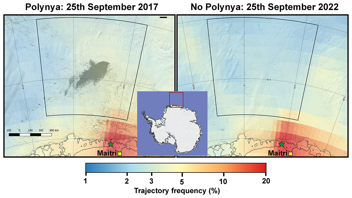
Figure 1 Study area and wind-trajectory patterns. (a) Maud Rise Polynya during its largest recent opening on 25 September 2017, detected with Moderate Resolution Imaging Spectroradiometer (MODIS) on NASA's Aqua satellite (from NASA Worldview, https://worldview.earthdata.nasa.gov/, last access: 1 April 2026) Imagery © 2026 NASA. The polynya is visible as the dark, open-water feature amidst the surrounding white sea ice (b) MODIS Satellite imagery taken on the same day in a non-polynya year, 25 September 2022. The MODIS corrected reflectance imagery provides a true colour representation where the open ocean appears dark gray or black, while sea ice and clouds appear white or light gray. Images are overlaid with the trajectory frequency of back-trajectories ending at the Djupranen ice core site (green star) from June to October in 2017 and 2022, respectively (see methods). The Indian Maitri Station is marked by a yellow square. The colourmap is on a logarithmic scale. The inset shows the location of the main map. Grounding line and calving front are marked (Matsuoka et al., 2015).

Following this dramatic episode, the Maud Rise region has exhibited intermittent polynya activity, typically manifesting as halos of reduced sea ice concentration (Lindsay et al., 2004; McHedlishvili et al., 2022). However, the phenomenon garnered renewed attention when a large polynya exceeding 40 000 km² reappeared during the two winters of 2016 and 2017 (Jena et al., 2019). Early polynya studies focused primarily on documenting polynya occurrence and extent through satellite imagery (Carsey, 1980; Comiso and Gordon, 1987; Zwally et al., 1985), while more recent works have attempted to unravel the complex mechanisms controlling polynya formation and maintenance (de Lavergne et al., 2014; Wilson et al., 2019). Satellite observations have revealed that open-ocean polynya formation often follows a characteristic pattern, beginning with the appearance of small-scale openings that can rapidly expand under favourable conditions, such as wind-driven upwelling (de Lavergne et al., 2014; Jena et al., 2019), baroclinic instabilities (Akitomo, 2006; Campbell et al., 2019), and deep warm water intrusions (Gülk et al., 2024; Heuzé et al., 2021). However, the precise triggers initiating this process remain incompletely understood, because the relative importance of these processes likely varies temporally and may be interconnected (Campbell et al., 2019; McPhee, 2003; Narayanan et al., 2024), and also because large polynya openings are rare and satellite-based observations range only for the past few decades, limiting the observational opportunity. Similarly, model-based assessments are limited in their ability to understand polynya formation in the weakly stratified Southern Ocean (Heuzé et al., 2013; Sallée et al., 2013). This modelling challenge hampers our ability to assess both the role of polynyas in natural climate variability and their potential responses to future climate change.

To obtain longer polynya records, Goosse et al. (2021) examined surface mass balance (SMB) records reconstructed from six ice cores and two automatic weather stations. In these records, they observed increased snowfall during the 2016–2017 MRP opening and assumed that similar anomalies occurred during the past MRP opening periods. Their study constructed a polynya index using two data assimilation approaches and one statistical method to reconstruct historical climate states based on SMB reconstruction from ice cores. Their study found multiple polynya openings since 1250 CE but observed that large polynya openings are rare. However, they rely only on snow accumulation records, which can be influenced by many factors other than polynya occurrences. The polynya signal in their ice-core SMB records is also weak compared to natural atmospheric variability, making it difficult to distinguish polynya-induced anomalies from SMB caused by other climatic fluctuations. The short instrumental record from automatic weather stations prevents a robust calibration of polynya reconstructions, increasing the risk of false positives (unrelated high snowfall events misinterpreted as polynya activity) and false negatives (missed polynya events). Additionally, the ice-core and instrumental records they used were collected from a large region, including the Weddell Sea sector and the ice sheet inland, where the surface elevation exceeds 2000 m a.s.l. (meter above sea level), which can hardly reflect changes in the vapour sources in the MRP regions directly (Fig. 1).

To overcome the limitations of the previous study, we develop a novel, multi-proxy approach to reconstruct past MRP activity using a high-resolution ice core, IND-36/9, from Djupranen Ice Rise in coastal Dronning Maud Land. While polynya opening results in increased heat and moisture exchange, the polynya years, characterised by a decrease in sea ice cover, also result in increased sea salt production. These signatures can be carried to the coastal region of Antarctica and deposited in the low-elevation ice shelves and ice rises. The back-trajectory analysis (Sect. 2.5) clearly indicates the direct atmospheric link between MRP and the IND-36/9 core site (Fig. 1). Our ice core site is situated within ∼1000 km of the typical MRP location, close enough to potentially capture atmospheric signatures transported from polynya formation near the Maud Rise. By combining records of snow accumulation, water isotopes, and major ion concentrations, we aim to provide a more robust reconstruction of polynya activity. This approach leverages the strengths of selecting an ideal core site and employing multiple proxies to overcome the limitations of single-proxy reconstructions, thereby capturing the complex signatures of polynya events that extend beyond the last few decades, when satellite and instrumental records are available.

2 Study Area and Methods

2.1 Study area

The DML coast is characterised by distinct topographic features like ice rises having associated local ice flow, climate regime and SMB variability (Drews et al., 2015; Goel et al., 2017; Lenaerts et al., 2014; Matsuoka et al., 2015; Pratap et al., 2022; Rignot et al., 2019). As part of the Indo-Norwegian project MADICE, an ice core was drilled on the summit of the Djupranen Ice Rise (70.18° S, 9.18° E; elevation 321 m a.s.l.), at the western margin of the Nivlisen Ice Shelf in coastal Dronning Maud Land (DML), East Antarctica (Fig. 1). Our site survey found that this ice rise summit has been at the current position at least in the past few millennia (Pratap et al., 2022). This location also offers several advantages for polynya reconstruction: its high SMB allows annual layer counting (Dey et al., 2023) and its coastal proximity may provide sensitivity to maritime signals (Ejaz et al., 2021; Wauthy et al., 2024), while its elevation causes insignificant surface melt and local noise while maintaining regional signal strengths (Dey, 2023). Its position is also within primary atmospheric transport pathways from the Maud Rise region (Fig. 1).

2.2 Ice core: from the field to the laboratory

The drill site of the Djupranen ice rise was located at its summit, based on analysis of satellite altimetry data and satellite image analysis, followed by an ice-penetrating radar survey (Pratap et al., 2022). The radar survey also shows a flat bed topography below the summit (Goel et al., 2026) and the presence of Raymond arches, indicative of a relatively stable summit position in the past (Goel et al., 2020). The ice core was drilled using an electromechanical ice core drilling system (Model D2, GeoTec, Japan). Over nine days, a 122 m ice core (IND 36/B9; hereafter IND36/9) was retrieved. The drilled ice core sections were sealed in high-density polyethylene core bags, packed in expanded polypropylene boxes, and stored in a reefer container at −20 °C until their transport to the National Centre for Polar and Ocean Research (NCPOR), Goa, India, where samples were stored in the in-house Ice Core Laboratory maintained at −20 °C. The ice cores were processed in the −15 °C core processing facility at NCPOR. The cores were initially cut into 3.5 cm thick, 10 cm wide slabs for line scanning and then subsequently sub-sampled at 5 cm resolution for stable isotope and chemical analysis. The samples for chemical analysis were cut into cuboids; the three dimensions of the samples were measured using a calliper and weighed using a weighing balance. The density for the samples was calculated as mass divided by the volume of each sample. The error in measuring the sample dimensions was ±0.5 mm, while the weighing balance's uncertainty was ±0.1 g for measurements up to 100 g. As a result, the density measurements have a propagated uncertainty of 5 %.

Major inorganic anions (Cl⁻, ${\mathrm{SO}}_{\mathrm{4}}^{\mathrm{2}-}$, MSA⁻ and ${\mathrm{NO}}_{\mathrm{3}}^{-}$) and cations (Na⁺, ${\mathrm{NH}}_{\mathrm{4}}^{+}$, K⁺, Mg²⁺, and Ca²⁺) were measured in the samples using an ICS 5000+ ion chromatograph (Thermo Dionex) equipped with a conductivity detector. Anions were separated on an AS11 (2 mm) column with potassium hydroxide as eluent and an AG11 (2 mm) guard column with AERS 500, 2 mm suppressor. Cations were separated on a CS17 (0.4 mm) capillary column with methane sulphonic acid as the eluent and the CG17 (0.4 mm) capillary guard column with a CCES 300 capillary suppressor. A 10 mg L⁻¹ stock solution of Na⁺, ${\mathrm{NH}}_{\mathrm{4}}^{+}$, K⁺, Ca²⁺, and Mg²⁺ was mixed and then diluted with MiliQ ultrapure water to prepare standards for cation exchange chromatography. The anion standards were prepared from 10 ppm stock solutions of MSA⁻, Cl⁻, ${\mathrm{SO}}_{\mathrm{4}}^{\mathrm{2}-}$, and ${\mathrm{NO}}_{\mathrm{3}}^{-}$. The dilutions were conducted volumetrically and were freshly prepared within a few days of each run, ranging from 5 ppb to 1 ppm. Eight standards were selected from this range for calibration. Before analysis, the ice core samples were melted in a Class 100 clean room. The analytical precision for all ions was better than 10 %.

The ice core samples were analysed for oxygen and hydrogen isotopic ratios at NCPOR using a Triple Isotope Water Analyser (TIWA-45EP from Los Gatos Research, USA), which works on the principle of off-axis integrated cavity output spectroscopy (OA-ICOS). The melted ice core samples were introduced into the TIWA-45EP without sample conversion through a PAL HTC-xt auto-injector (CTC Analytics) equipped with a heated (∼85 °C) injector block (LGR) (Berman et al., 2013). Using a Hamilton 1.2 µL, zero-dead-volume syringe, samples were injected into the injector block and evaporated for direct isotope analysis. Measurements were completed at a speed of ∼90 s per individual injection. To eliminate sample-to-sample memory, a total of nine injections were made, with the first three being discarded for analysis. The last six injections were averaged to produce a single, high-throughput (HT) sample measurement. One commercially available working standard from LGR1C and two in-house laboratory standards (CDML1 and HL1) with known isotopic composition, spanning the entire range of our sample measurements (−46.19 ‰ to −19.49 ‰ for δ¹⁸O and −362.85 ‰ to −154.0 ‰ for δD) were analysed routinely as reference waters after every five ice core samples to check the instrument performance. Laboratory standards are calibrated on the VSMOW/SLAP scale. The external precision obtained using our laboratory standards (CDML1 and HL1) for δ¹⁸O was ±0.046 ‰ and ±0.068 ‰, respectively, and for δD was ±0.32 ‰ and ±0.23 ‰ (1σ standard deviation) for 30 samples. Replicate analyses performed based on ten samples yield repeatability of ±0.76‰ for δD and ±0.09‰ for δ¹⁸O. All the raw instrumental OA-ICOS data were processed in the LGR post-analysis software. Any measured injection with water number density outside the manufacturer's suggested range of 2–$\mathrm{4.5}\times {\mathrm{10}}^{\mathrm{16}}{\mathrm{H}}_{\mathrm{2}}\mathrm{O}\mathrm{molecules}{\mathrm{cm}}^{-\mathrm{3}}$ was discarded. Injections with incomplete evaporation were detected by examining the standard deviation of the measured water number density (σ_nmeas) as reported by the instrument (Berman et al., 2013). Processed raw data directly gives δ¹⁸O and δD, which are further used to calculate deuterium excess [$\text{d-excess}={\mathit{\delta }\mathrm{D}}_{\text{ice}}-\mathrm{8}\times {{\mathit{\delta }}^{\mathrm{18}}\mathrm{O}}_{\text{ice}}$].

2.3 Chronology development

The chronology of the IND36/9 core is based on a multiproxy approach involving annual layer determination from the stratigraphy of δ¹⁸O, major ions, and pixel intensity data from the line scanner, following Dey et al. (2023). The core has experienced limited surface melt, with annual melt proportion varying between 0 % and 4.4 %, with a median melt proportion of 0.25 % (Dey et al., 2023). Since diffusion in the firn attenuates high-frequency water-isotope information in ice cores (Firn Symposium team, 2024), even in high accumulation sites of coastal Antarctica (Mahalinganathan et al., 2022), we diffusion-corrected our water isotope records following Jones et al. (2023) as detailed in (Sect. S1 and Fig. S1 in the Supplement). The shift in seasonal peaks in our corrected record is less than 5 cm, which falls within the sampling interval of 5 cm and is therefore insignificant in affecting the accuracy of the chronology.

A five-point smoothing was applied to the pixel intensity data to simplify annual layer counting and reduce noise in the record. We also used age tie points of known volcanic eruptions identified from non-sea-salt sulphate (nssSO₄) peaks, as well as the tritium bomb peak of 1962. Volcanic indicators (nssSO₄) have been used to identify specific, dated volcanic eruptions, allowing us to reduce the uncertainties resulting from the relative dating procedure. However, unambiguous eruption identifications are challenging in ice cores from coastal regions, where the nssSO₄ background signals are commonly highly variable due to the proximity of the ocean and ocean-related MSA products (Philippe et al., 2016).

A preliminary chronology was obtained from the annual counts, which was then refined using the nssSO₄ peaks (Fig. 2) from the well-established volcanic eruptions of Pinatubo (1991), El Chichon (1982), Agung (1963), Cerro Azul (1932), Santa Maria (1902), Krakatoa (1882), Cosiguina/Babuyan (1834), Tambora (1815) and unknown volcanic eruption (1809). Similar to Dey et al. (2023), we refined the chronology between the volcanic and Tritium tie points using the StratiCounter algorithm (Winstrup et al., 2012). The manual counts provide a basic framework from which StratiCounter develops and refines its statistical characterisation of annual layers, enabling adaptation to varying layer properties with depth (Winstrup et al., 2012). To minimise reliance on initial manual inputs, we conducted multiple iterations using refined layer templates derived from previous algorithm outputs. The chronology of the IND36/9 ice core provides a robust temporal framework that extends back to 1774 CE at a depth of 122 m (Fig. 3).

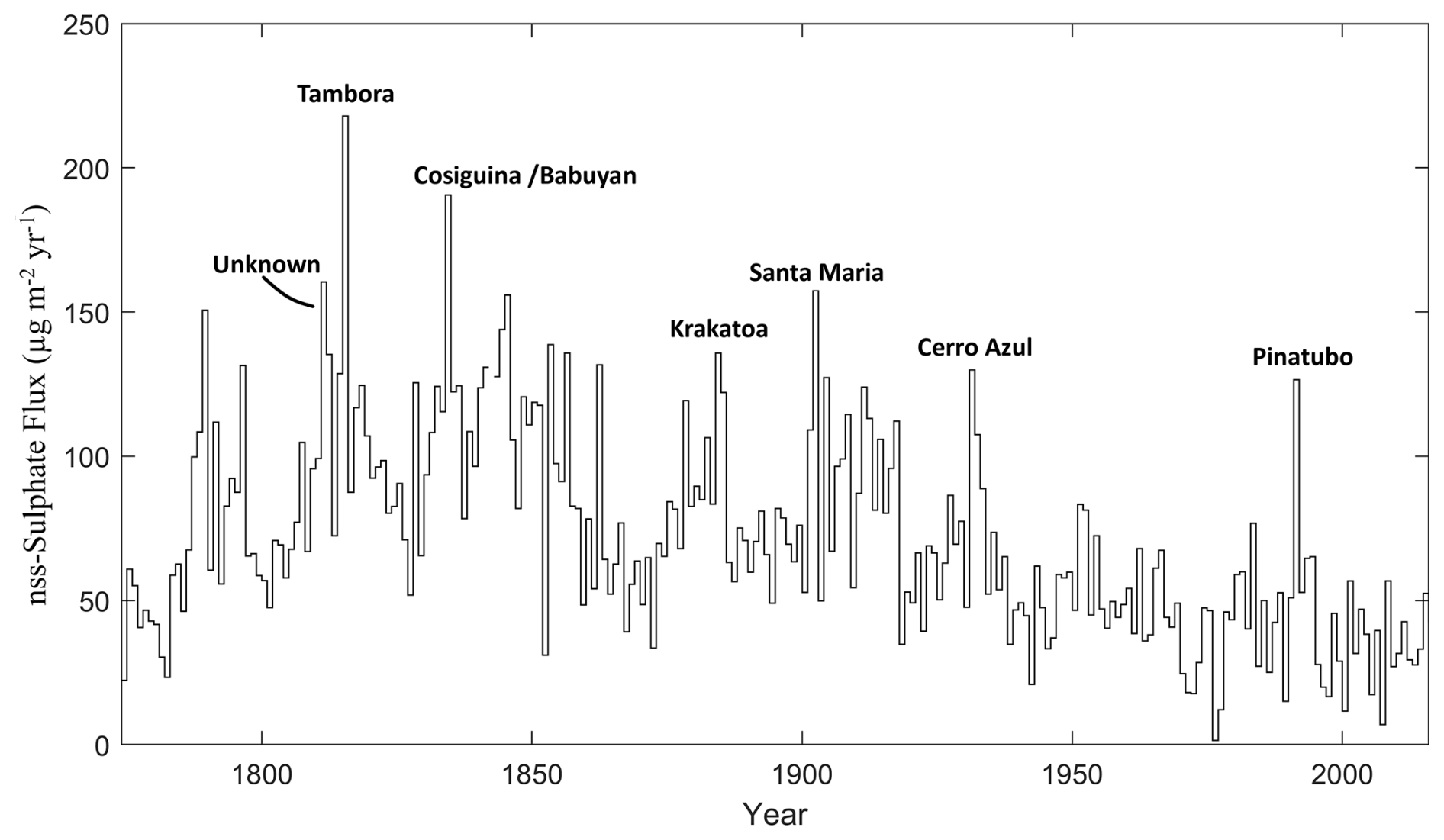
Figure 2 Tie points for ice core chronology. Volcanic events are identified from the non-sea-salt sulphate flux records. Only major volcanic events used as age tie points for reconstructing the chronology are marked.

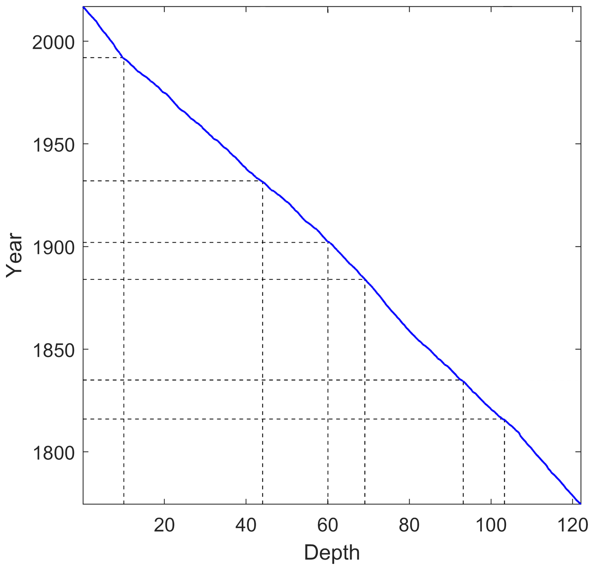
Figure 3 Age-depth scale for the Djupranen ice core. Tie points used for chronology (Fig. 2) are shown with dashed lines. Major time markers are shown using the black dashed lines. Minimal deviation from the intersection points of the vertical and horizontal lines indicates the robustness of the chronology.

2.4 Satellite-based polynya metrics

We followed Heuzé et al. (2021) to define the “polynya-prone” region of the Weddell Sea (6° W–12° E, 68–60°S, approximately 600 km×900 km), focusing on the winter and early spring months (1 June–31 October). This region was selected based on historical observations of polynya formation and its significance in Antarctic bottom water production (Campbell et al., 2019; Heuzé et al., 2021). Polynya activity was quantified using two independent metrics derived from satellite data. These metrics complement each other to provide a comprehensive assessment of polynya dynamics.

To quantify the polynya metrics, we use sea ice concentration data derived from passive microwave measurements using the NASA Team algorithm (Comiso and Nishio, 2008), processed at a spatial resolution of 25 km×25 km per pixel. The first metric, Polynya Days, represents the annual count of days (between 1 June and 31 October), with a minimum sea ice concentration in the polynya-prone region below 60 %. The second metric, Cumulative Polynya Area, measures the total extent of all polynya occurrences within a year (1 June–31 October). This was calculated by summing the daily open water areas within the polynya prone region, defined as the cumulative sum of pixel area with sea ice concentration below the 60 % threshold. The combination of these metrics allows us to characterise both the temporal persistence and spatial extent of polynyas, providing insights into their formation mechanisms and potential impact on regional oceanographic processes.

2.5 Air mass trajectory modelling

The HYbrid Single-Particle Lagrangian Integrated Trajectory (HySPLIT) model, developed by the NOAA Air Resources Laboratory (ARL), provides a means of generating back trajectories to identify the source of moisture uptake for precipitation (Markle et al., 2012). We used HYSPLIT version 5.3 for back trajectory computations, initialized with conditions from the 2.5 by 2.5-degree resolution NCEP/National Center for Atmospheric Research (NCAR) reanalysis data for the period 1948–2016. While these coarse-resolution meteorological fields inherently smooth sharp coastal topographical features and complex local wind patterns around them, which are characteristic of coastal DML, they are still sufficient for resolving regional-scale atmospheric transport pathways. Forward trajectories were run for 240 h (10 d), initialised every hour, starting over the polynya-prone region of the Weddell Sea. Groups of forward trajectories were computed with initial altitudes of 100, 200, 300, 400, and 500 m above ground level (m a.g.l.), and in all cases, the vertical velocity from the meteorological data was used as the input for vertical motion.

We calculated trajectory density from multiple trajectories using HYSPLIT, because individual trajectories are highly sensitive to meteorological uncertainties, turbulence, and small initial condition variations, often leading to misleading or unreliable airflow pathways and potential position errors of up to 20 % of the distance travelled. It also aids in differentiating between local circulation patterns and regional-scale flow features (Dorling and Davies, 1995) and has been previously applied to interpret polar ice core paleoclimate records (Dixon et al., 2012; Ejaz et al., 2021; Neff and Bertler, 2015). We calculated air mass transport densities for each year 1979–2016 from the HySPLIT output. The trajectory densities in each equal-area (1° by 1°) pixel were summed and divided by the total number of air mass trajectories.

3 Results

3.1 Identification of polynya years in satellite data

Satellite imageries are crucial for polynya studies as they provide continuous, high-resolution observations of sea ice dynamics, allowing researchers to monitor polynya formation, extent, and variability over time. Satellite observations spanning four decades reveal distinct periods of polynya activity in the Weddell Sea region since 1979 (Fig. 4). The most notable and well-documented event occurred during 1974–1976, when the polynya reached an exceptional size of 300 000 km² (Carsey, 1980). This event, often referred to as the Great Weddell Polynya, represented a significant perturbation to the regional ocean–atmosphere system and has served as a benchmark for subsequent polynya observations. Following this major event, several smaller polynyas and polynya-like features (“halos”) have been observed during the late 1980s to early 1990s and early 2000s (Heuzé et al., 2021). The two independent metrics used for polynya detection – Polynya Days and Cumulative Area – reveal distinct but complementary temporal patterns. This dual-metric approach enables a more comprehensive understanding of polynya dynamics than either metric alone could provide. While the magnitudes of these metrics do not exhibit direct correlation (r=0.42, p<0.01), both metrics successfully identify known major polynya/halo events between 1979 and 2016, and provide unique insights into their temporal and spatial characteristics. The Polynya Days metric effectively captures persistent small-scale features, while the Cumulative Area metric better represents brief but large openings. While the record of polynya openings from satellite imagery provides crucial insights, their influence on coastal Antarctic ice cores could depend majorly on atmospheric transport.

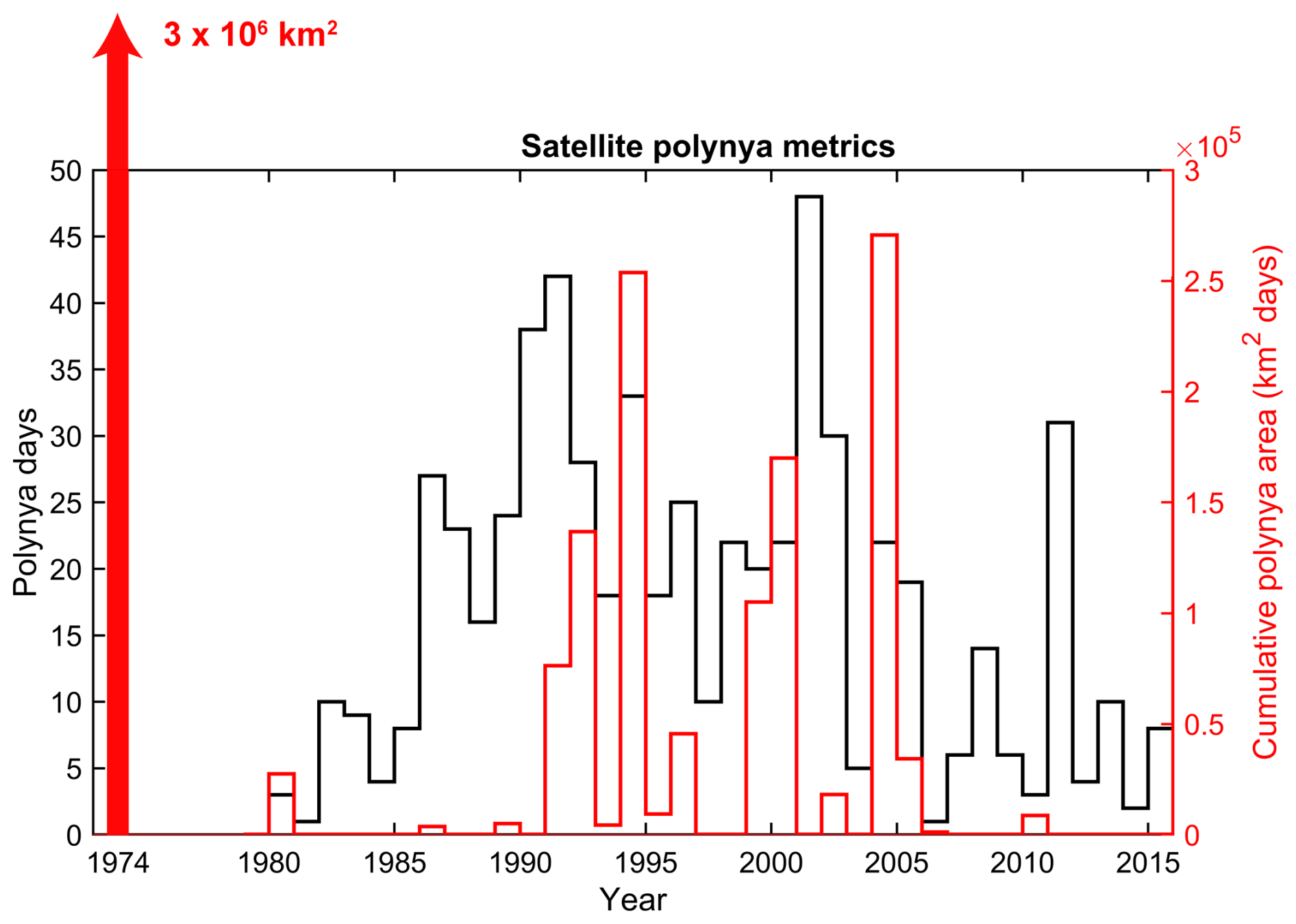
Figure 4 Satellite polynya metrics. Two different annual metrics of satellite-derived polynya occurrence. Since the polynya is highly dynamic temporally and spatially, the metrics do not show a one-to-one resemblance. The red vertical bar shows the 1974–1976 polynya event, which reached a peak extent of approximately 300 000 km² (Carsey, 1980), more than ten times of the maximum cumulative polynya area observed between 1979–2016.

3.2 Air mass transport patterns

We use forward air trajectory analysis to examine the transport pathways and determine whether polynya-derived signals can reach and be recorded in the ice cores. This approach allows us to trace the path of air masses from the polynya-prone area to potential ice core sites, providing insight into which locations are most likely to capture polynya signals. Forward trajectory analysis reveals consistent and well-defined transport pathways from the Maud Rise region to coastal Dronning Maud Land (Fig. 5). Frequency analysis shows that our study site (1°×1° box surrounding the ice core site) receives approximately 2 % of all trajectories originating from the MRP region, a statistically significant proportion (p<0.001) that indicates reliable capture of polynya-related atmospheric signals. This percentage remains relatively stable across different seasons and years, suggesting a robust atmospheric connection between the source and deposition regions. The trajectory density analysis indicates that our ice core location falls within a primary atmospheric transport corridor originating from the MRP region. This corridor exhibits enhanced stability during the winter months when polynya formation typically occurs. However, trajectory calculations are susceptible to significant spatial error of 15 %–30 % of distance travelled (Draxler, 2008). Therefore, a combination of forward and backward trajectories would provide a better overview of the travel pathways. Our back-trajectory analysis (Fig. 6) further confirms the findings from the forward trajectory patterns, with ∼19 % of all trajectories reaching our ice core site having also traversed over the polynya prone region. We observe that air masses reaching our site also originate from more distant open-water areas (even during the winter months) in the Southern Ocean. However, these distal sources remain relatively consistent across the study period and are located significantly further from the IND-36/9 site compared to the polynya-prone region. Consequently, these background marine inputs are less likely to drive the synchronized, high-magnitude anomalies observed across all proxies, particularly the sharp increases in ssNa flux, that characterize the polynya years. Trajectory analysis of the transport pathways, therefore, confirms that winds can carry polynya-derived signals from the open water to our study site and preserve them in the ice core records, regardless of polynya presence.

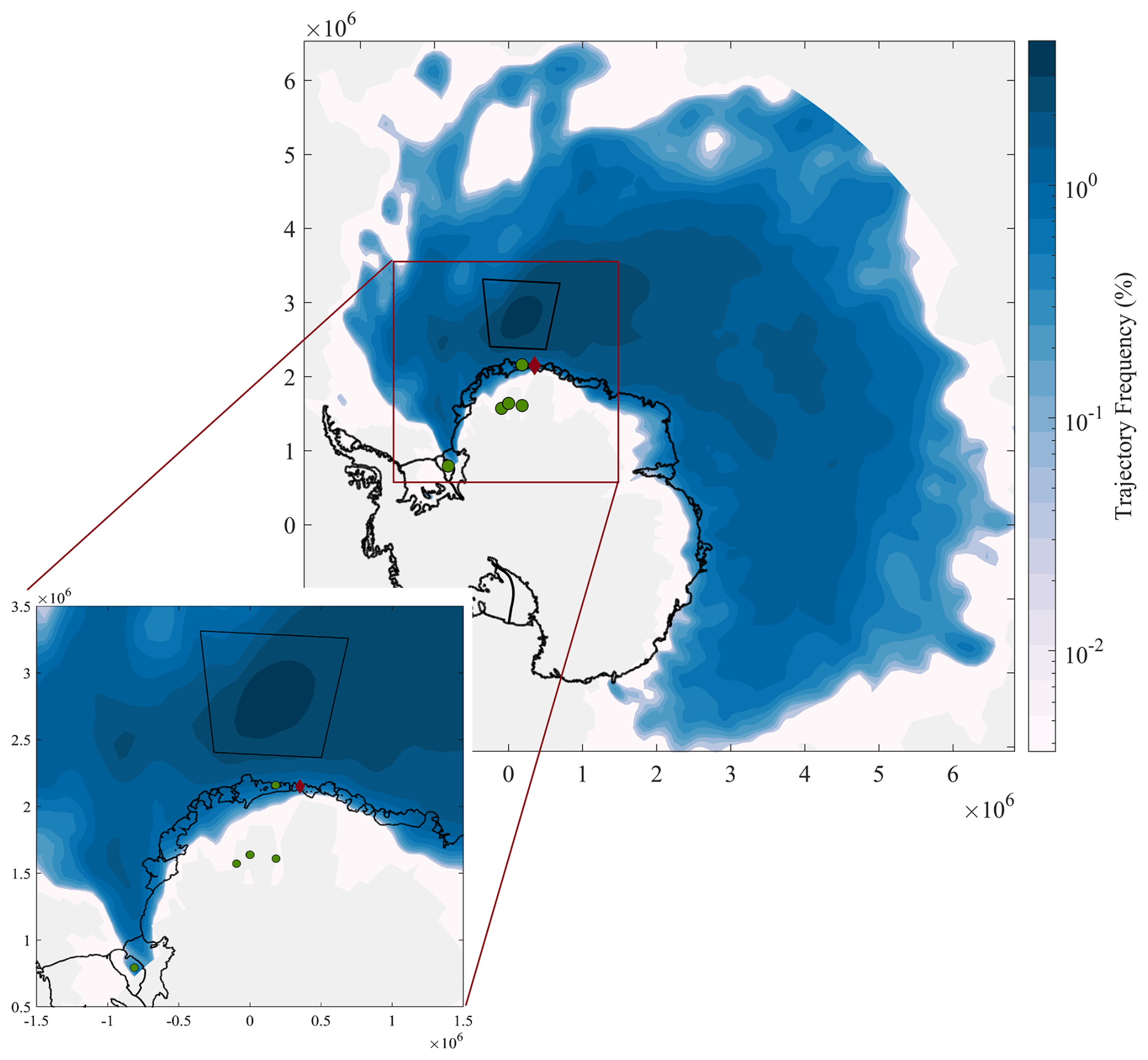
Figure 5 Airmass transport pathways originating from MRP: Trajectory frequency of forward trajectories originating over the polynya-prone region (Heuzé et al., 2021) of the Weddell Sea, showing the prevalent transport pathway during the winter to early spring months for the period 1948–2016. A significant proportion of the trajectories end over our ice core site (red diamond). Location of ice cores used by Goosse et al. (2021) are shown with green circles. The black trapezium shows the polynya prone regions. The gray region shows area with no trajectories.

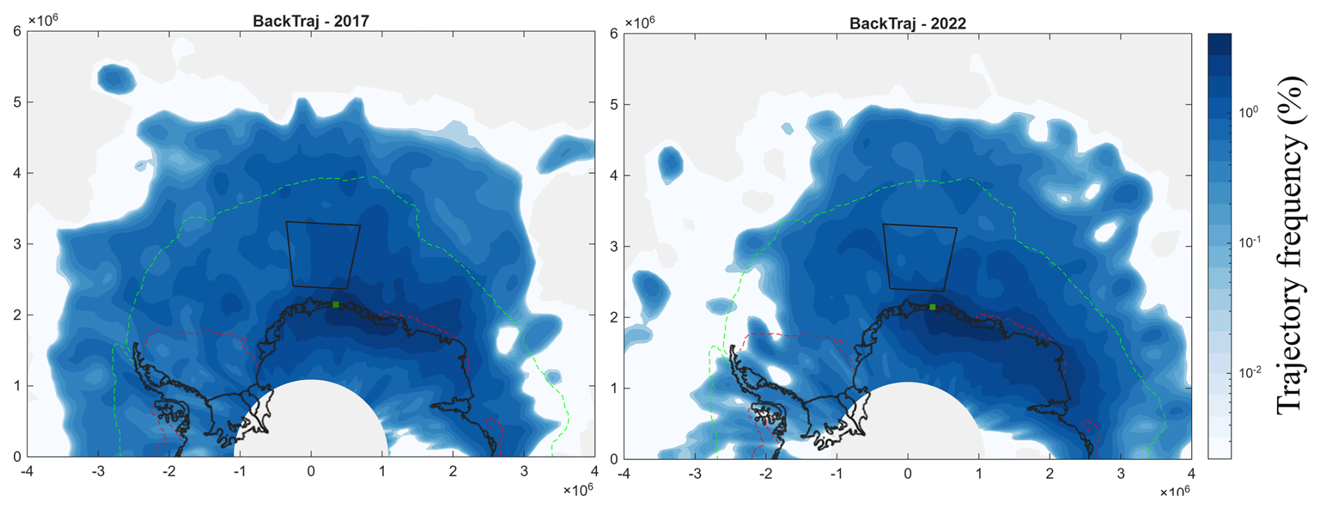
Figure 6 Airmass transport pathways ending at the ice core site: Trajectory frequency of back trajectories originating from the ice core site during a well-known polynya year (2017; left) and a non-polynya year (2022; right) is shown. The trajectory frequency pattern during both years is very similar, indicating a consistent transport pathway during most of the years and suggesting that our ice core records activity over the polynya-prone region of the Weddell Sea (black trapezium) in all years. The gray region shows areas with no trajectories. The dashed lines show the NSIDC median sea ice extent for 1980–2010, with green indicating September (maximum) and red representing February (minimum) sea ice extent.

3.3 Development of the polynya index

3.3.1 Ice core record and proxy selection

The ice core proxy dataset from 1774–2016 exhibits distinct variability across all measured properties. We choose four major proxies for developing our polynya index: sea-salt sodium (ssNa), deuterium excess (d-excess), δ¹⁸O, and snow accumulation (Figs. 7a and S2 in the Supplement). Sodium concentration ranges from a low of 19.1–218.6 ppb, with a mean value of 89.9 ppb. Some periods show sustained higher values, such as the late 1700s and early 1800s, while others, including the late 19th and 20th centuries, display more variable levels. D-excess varies between −1.8–10.8 ‰, with a mean of 4.3 ‰, showing notable peaks in the late 19th century and sharp declines in the early 20th century. δ¹⁸O values fluctuate between −21.6 ‰ to −15.6 ‰, with a mean of −17.8 ‰, displaying alternating periods of enrichment and depletion, including a gradual decline over recent decades. Annual snow accumulation ranges from 0.12–0.83 m w.e., with a mean of 0.39 m w.e., exhibiting distinct fluctuations, including lower values in the early 20th century and a more variable pattern in recent decades.

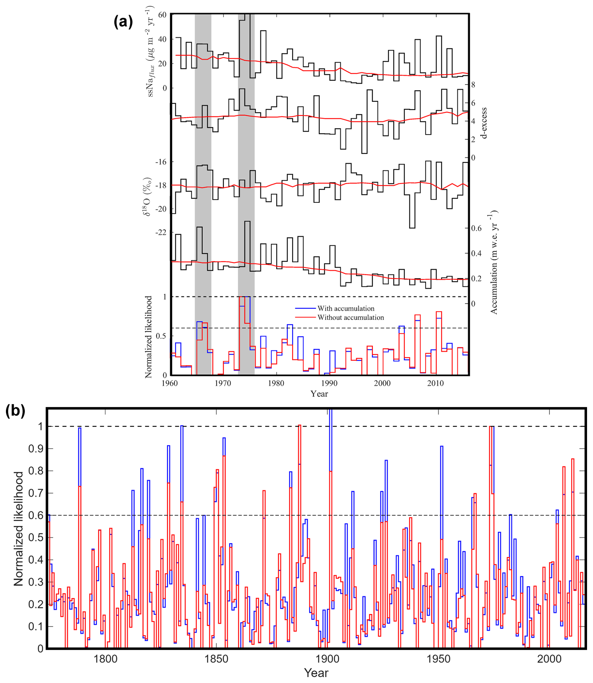
Figure 7 (a) Ice core proxies and polynya identification. Annual variability of selected ice core proxies and polynya index from 1960–2016. The red curve is the moving median over a 30 year window. The two known polynya events of 1964 and 1974–1976 are marked with gray patches. (b) Ice core derived polynya indices: Ice core derived polynya indices in the past 250 years using the anomalies in the annual record of four ice-core proxies: Na, deuterium excess, δ¹⁸O, and snow accumulation. To test the dependence of the polynya index on snow accumulation, we calculate two indices, one using snow accumulation (blue curve) and another without (red curve). The two indices behave similarly over the entire time period; however, the index without snow accumulation shows a higher range of variability.

The opening of a polynya results in increased heat and moisture exchange between the warm, open water and the cold air. Therefore, during polynya years (decrease in the sea ice cover), there is also an increase in local precipitation in the Weddell Sea region (Moore et al., 2002) and resultant snow accumulation further inland (Goosse et al., 2021). The water isotope ratios of precipitation are often related to temperature at the precipitation site (Ejaz et al., 2022; Naik et al., 2010) and the distance of transport (Goursaud et al., 2017; Klein et al., 2019), and the pattern of annual mean water isotopes (δ¹⁸O) of precipitation associated with polynya formation would relatively be similar to that for increased temperature from the heat exchange due to polynya opening and shorter transport distance, especially over a coastal site. During winter and spring, the opening of the MRP exposes open seawater ($\text{SST}\approx -\mathrm{1.5}\mathrm{°}\mathrm{C}$) directly to extremely cold polar air masses ($T<-\mathrm{15}\mathrm{°}\mathrm{C}$) blowing off the ice sheet or driven by cyclonic circulation. Because these polar air masses are cold and dry, the actual atmospheric vapor pressure ($e_{\mathrm{a}}=\mathrm{0.0611}\times \text{RH}\times {\mathrm{10}}^{\frac{\mathrm{7.5}\times T}{\mathrm{237.3}+T}}$) is exceedingly low. As a result, the relative humidity normalized to the sea surface temperature ($\text{rhs}=\frac{e_{\mathrm{a}}}{e_{\text{sat}}\left(\text{SST}\right)})$ drops drastically. This large humidity deficit at the air–sea boundary layer drives rapid, highly kinetic, non-equilibrium evaporation, which is further amplified by the high-wind environments typical of DML cyclonic activity and katabatic flow, which sweep away the boundary layer and maintain this dry, highly undersaturated state. This results in higher d-excess in the evaporating moisture, injecting a localized vapour plume with positive d-excess anomalies directly into the coastal precipitation during polynya openings.

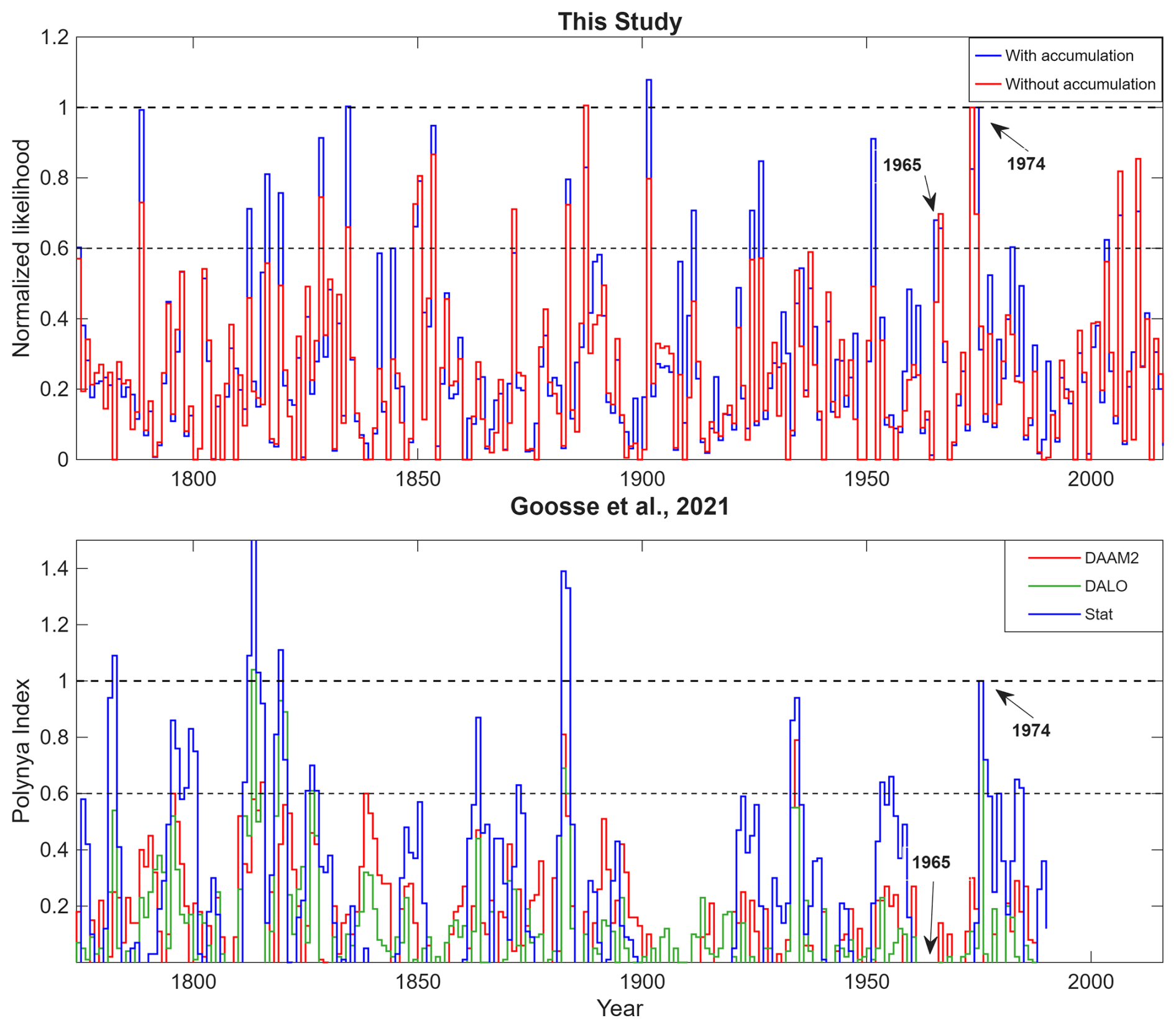
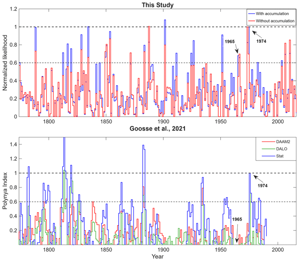
Figure 8 Comparison of the polynya indices. Polynya indices reconstructed in this study (upper panel) are shown with the polynya indices from Goosse et al. (2021) (lower panel). The polynya indices from Goosse et al. (2021) are based on six surface mass balance records using data assimilation with two control simulations performed with the SPEAR (Seamless system for Prediction and EArth system Research) global climate model, SPEAR_AM2 (DAAM2; Blue) and SPEAR_LO (DALO; green), and a simple average of the standardized time series (Stat, red). The known polynya events of 1964 (1965 in our record and absent in Goosse et al. (2021) and 1974–1976 (1974 in our record and 1975 in Goosse et al., 2021) are labelled.

While sea ice typically acts as a physical barrier to air–sea exchange, a polynya creates a localized window for enhanced aerosol production via multiple distinct mechanisms. First, the open-water surface provides a direct source where high-speed cyclonic winds and storm activity trigger bubble-bursting processes, injecting sea-salt particles into the marine boundary layer. Second, extensive open water polynyas can also act as a large factory for sea ice production, comparable to the production of the largest coastal polynyas (Zhou et al., 2023). Previous studies have shown that the surface of fresh sea ice, including frost flowers, is an important source of sea salt to the Antarctic, and the production of frost flowers is controlled by the amount of new sea ice production (Wolff et al., 2003). Furthermore, blowing snow across these newly formed, brine-wetted ice surfaces facilitates the sublimation of salty snow particles, which is also the major source of sea salt aerosol to the inland sites (Frey et al., 2020). Because these processes occur proximately to the drilling site and are situated directly along the atmospheric trajectories identified in Fig. 6, they result in high-magnitude pulses of ssNa that are chemically distinct from the far, year-round open-ocean baseline. We however use ssNa flux instead of concentration to mitigate the potentially confounding effects of varying annual snow accumulation rates. By using flux, we ensure that a dilution effect during high-snowfall years doesn't artificially lower our ssNa signal, and conversely, that a low-snowfall year doesn't create a false peak.

3.3.2 Development of the integrated polynya index

To reconstruct past MRP activity, we developed a multi-proxy index using a cumulative-anomaly approach, calculated as the means of rolling z-scores. This allows us to isolate anomalies that are synchronized across proxies from long-term climate trends. We use four independent proxies: sea-salt sodium (ssNa) flux, δ¹⁸O, deuterium excess (d-excess), and annual snow accumulation rates for our polynya index calculation. Prior to index calculation, all proxies are scaled to 0–1 to remove bias toward proxies with greater variability. For each proxy, we first calculate a 30 year rolling z-score to identify annual departures from the local background state. This accounts for non-stationary signals in the 250 year record, such as the gradual depletion of water isotopes or recent decreases in snow accumulation rates. As explained in Sect. 3.3.1, MRP openings are linked to positive anomalies in ssNa flux, δ¹⁸O, d-excess, and annual snow accumulation rates; therefore, we used only positive z-scores for the calculation. Negative z-scores were set to zero to prevent them from cancelling out physically significant peaks in other proxies. To test the dependence of the polynya index on snow accumulation, we calculate two versions of the index: one using all four selected proxies and another excluding annual snow accumulation rates. The polynya index is a mean of all individual rolling z-scores, which is then normalized so that the final values are such that the largest known polynya opening of 1974–1976 is set to 1. A polynya year (a year when a polynya activity is recorded) is defined as a year in which the polynya index exceeds the likelihood threshold (0.6, 0.8, or 1). The polynya index is, therefore, an indicator of polynya occurrence from ice core observations and not a measure of the absolute extent or duration of the polynya events.

3.4 Past Maud Rise Polynya activity

Our ∼250-year reconstruction reveals complex and significant temporal variability in polynya occurrence, shedding new light on the long-term behaviour of the Maud Rise Polynya (MRP). We identified twenty-five potential polynya years from 1774–2016 (likelihood>0.6; Fig. 7b), with three events (1788, 1834 and 1901) exceeding the threshold of 1.0, indicating that these were events of possibly similar magnitude as the 1974–1976 polynya opening. The high index values for these events likely indicate that they were large-scale and persistent openings; however, exact quantification of the polynya extent is beyond the scope of this study. During the late 18th to mid-19th century, the polynya exhibited a high-frequency variability, frequently dropping to near-zero levels as seen in 1782 and the early 1800, while also producing moderate activity clusters above the 0.6 threshold in the 1810s and late 1820s. The late 19th century transitioned into a period of more consistent activity, with 1887 being a notable high-activity year exceeding 0.8. The early 20th century was marked by a prominent polynya in 1901 followed by significant bursts of activity exceeding the 0.60 threshold in 1911, 1924, and 1926. Mid-century activity was relatively suppressed, though a significant spike above 0.9 occurred in 1951. The lesser known 1964 polynya opening is also recorded in our polynya index (1965 in our polynya index); however, the likelihood is relative lower (>0.6) than the 1974–1976 event. Following the 1974–1976 event, the post-1980 era has generally shifted toward lower average values, though moderate spikes exceeding the 0.6 threshold occurred in 1982, 2003, 2006, and 2010, corresponding to known halo years.

4 Discussion

We compared our polynya index with those from Goosse et al. (2021) and found that the major polynyas identified in our study over the common time period are mostly identified in their reconstruction (Sect. S3 and Fig. S3 in the Supplement). This provides a degree of validation for both approaches, suggesting that they are capturing similar large-scale polynya events. However, our index shows enhanced sensitivity to polynya formations, identifying the polynya occurrence of 1964 (Fig. 8), even though with a lower likelihood. This low likelihood of the 1964 polynya is possibly due to the lower persistence as compared to the well-documented events during 1974–1976 (Meier et al., 2013). Furthermore, our index shows better performance in identifying transient polynyas and halos, which were missed in the reconstruction by Goosse et al. (2021). These shorter-lived or less intense polynya events, while not as dramatic as major openings, play a crucial role in regional oceanography and climate dynamics. Their detection provides a more comprehensive picture of polynya activity over time. Beyond chronological offsets, discrepancies between the two indices likely reflect differences in regional sensitivity and site selection. Our analysis of air mass transport frequency from the MRP regions shows a sink in the coastal regions of Dronning Maud Land, with a significant proportion of the trajectories reaching our study area. In contrast, four out of the six ice core sites used in Goosse et al. (2021) fall outside the primary sink of these trajectories (Fig. 5). This difference in site selection could be a major reason for the observed discrepancy between the two polynya indices. Ice cores from sites that rarely receive air masses from the polynya region may not be reliably used to reconstruct polynya events or may do so with reduced sensitivity. Whereas our ice core site is well located to capture the occurrence of the MRP opening, as it frequently receives air masses originating from the polynya region. However, Goosse et al. (2021) still manage to detect the large, multi-year polynyas as they lead to a widespread positive anomaly in precipitation over the coastal and continental region. Consequently, while our index captures both high-magnitude regional events (e.g., 1974) and more localized openings (e.g., 1964), inland records may only register the most extreme regional anomalies. This suggests that the lack of a perfect year-to-year correlation is not a limitation of the proxies themselves, but rather a reflection of the better spatial representativeness of the IND-36/9 site for capturing the nuances of the Maud Rise polynya system. Another possible reason for this observed difference in sensitivity could be the robustness of our multiproxy approach in identifying polynyas, as it is less susceptible to noise or artefacts in any single proxy. It is crucial to note that the observed differences in peak occurrences do not necessarily invalidate either dataset but rather highlight the complexity in reconstructing past polynya activity. These discrepancies underscore the challenges inherent in paleoclimate reconstruction and the potential complementarity of different methodologies in building a comprehensive understanding of past polynya dynamics.

Our polynya reconstruction aligns with and extends satellite era observations of MRP formation mechanisms. Recent studies have shed light on the complex interplay of oceanic and atmospheric factors controlling MRP formation and persistence (Campbell et al., 2019; Jena et al., 2019). However, extending these insights to longer timescales remains challenging. Our multi-century reconstruction offers a unique opportunity to explore the long-term drivers of MRP variability. Autonomous profiling float observations during 2016 and 2017 revealed that the MRP was initiated and modulated by the passage of severe storms, and the intense heat loss drove deep overturning within them (Campbell et al., 2019). Wind-driven upwelling of record strength weakened haline stratification in the upper ocean, thus favouring destabilisation. A recent study, however, highlighted the role of salt transport through northward Ekman transport as an additional mechanism of the polynya formation and these processes were driven by intensified eastward surface stresses during 2015–2018 (Narayanan et al., 2024). Therefore, it is crucial to understand the maritime climate variability during the polynya and non-polynya years. Our reconstruction shows alternation between polynya-active and quiescent periods, which may provide valuable context for assessing how future MRP behaviour may evolve under anthropogenic climate change. The temporal clustering of MRPs in our record possibly indicates that once favourable preconditioning develops, the region remains susceptible to repeated polynya openings over several years or decades. As global temperatures rise, projected changes in Southern Ocean wind patterns, sea-ice extent, and surface freshening may shift the thresholds required for deep convection, thereby altering both the frequency and persistence of MRPs. Understanding how atmospheric and oceanic conditions differ between the polynya and non-polynya periods identified in this study will be critical for refining projections. Integrating these insights with high-resolution coupled ocean–atmosphere models could help identify the physical thresholds and feedback governing MRP formation. Such integration is crucial for predicting how rare but climatically significant features such as the Maud Rise Polynya may influence Southern Ocean overturning, carbon exchange, and global climate in a warming world.

5 Conclusions and Outlook

We provide new insights into the temporal variability of Maud Rise Polynya, one of the largest and well-known open ocean polynyas, by integrating multiple proxies using an ice core from coastal Dronning Maud Land, representing the past nearly 250 years. We identified multiple polynya openings during the 1830s, 1880s, and 1970s. These clusters of polynya openings possibly correspond to a specific combination of atmospheric circulation patterns and oceanographic preconditioning, suggesting a more deterministic framework for MRP development. Over the 250 year record, we identify large events during 1833–1834 and 1911, which were comparable in magnitude to the documented 1974–1976 polynya, indicating that such openings are not isolated anomalies but represent recurring features of the Southern Ocean system. These events are characterised by proxy signatures consistent with modern polynya conditions, supporting the persistence of underlying formation mechanisms throughout the observational period. Conversely, the interval from 1920–1950, marked by a notable absence of polynya activity, coincides with documented changes in Southern Ocean circulation and atmospheric forcing. This prolonged quiescent phase provides valuable baseline information for assessing natural variability in MRP activity on multi-decadal timescales.

Our multiproxy approach significantly enhances the sensitivity of the reconstruction, particularly in detecting smaller-magnitude and shorter-duration events that may have been overlooked in previous studies. As a result, the reconstructed history reveals a more dynamic and variable pattern of MRP activity than previously recognised, with implications for understanding its role in ocean ventilation, carbon cycling, and regional climate variability. Our study reveals that synthesising paleoclimate records, modern observations, and modelling approaches can provide a robust foundation for advancing the understanding of the MRP as a critical and recurrent component of the Southern Ocean climate system.