Late Holocene stabilization of Conway Ice Ridge

Marine ice sheets are low-pass filters of climate variability that take centuries to millennia to adjust to interior and near-terminus changes in mass balance. Constraining these long-term changes from satellite altimetry and velocity observations that span only the last 40 years is a challenge. Here, we take a different approach, synthesizing different data sources to infer changes in the configurations of van der Veen and Mercer Ice Streams on the Siple Coast over the past 3000 years. Englacial radar data from Conway Ice Ridge reveal smooth, surface conformal layers overlying disrupted stratigraphy that suggest the van der Veen Ice Stream was 40 km wider over 3000 years ago. Englacial layer dating indicates that the ice stream narrowed to its present configuration between ∼3000 and ∼1000 years ago. Similarly disrupted stratigraphy and buried crevasses suggest that ice flowing from Mercer to Whillans Ice Stream across the northwestern tip of the ridge slowed shortly after van der Veen narrowed. Using an ice-flow model capable of simulating shear-margin migration, we evaluate whether small changes in ice thickness can lead to large changes in shear-margin location. Our results suggest that the tip of Conway Ice Ridge is sensitive to ice thickness change, and that when the basal strength at the tip of the ridge increases with the ice thickness above flotation, the ice-stream shear margin locations can change quickly.

1 Introduction

The Siple and Gould Coast ice streams are some of the most well-studied ice-stream systems in Antarctica. Monitoring programs dedicated to understanding the physical controls of streaming ice flow through these tributaries into the Ross Ice Shelf date back to the International Geophysical Year (1957–1958; i.e. Crary, 1961; Crary et al., 1962). This early work inspired several large-scale projects (Ross Ice Shelf Project, Siple Coast Project, TAMSEIS, drilling of Whillans Subglacial Lake, Mercer subglacial Lake, and SWAIS2c) and studies (MacAyeal and Thomas, 1979; Alley and Whillans, 1991; Bindschadler, 1993; Clough and Hansen, 1979; Tulaczyk et al., 2014; Priscu et al., 2021) that have shaped fundamental understanding of the mechanics that control streaming flow and flow history in the Ross Sector during the Holocene (Anandakrishnan and Alley, 1997; Tulaczyk et al., 2000; Bindschadler et al., 2003; Catania et al., 2006; Winberry et al., 2009, 2011, 2014; Zoet and Iverson, 2020; Siegfried et al., 2023). The relatively simple geometry, but varied thermomechanical behavior of the Siple Coast ice streams over the relatively recent past (since the Last Glacial Maximum) combined with the rich paleo and modern datasets make the Siple and Gould Coast ice streams a compelling natural laboratory for understanding ice-stream evolution.

The mid to late Holocene epoch (11.7 ka BP–present) is generally considered to be a period of relative climate stability with variations in global average temperatures of less than (±0.5 °C) and relatively small changes in global ice volume (Jones et al., 2022). However, growing evidence suggests that the West Antarctic Ice Sheet was smaller than the present configuration during the mid-Holocene (8.2–4.2 ka) and subsequently re-advanced over the last several thousand years (Kingslake et al., 2018; Venturelli et al., 2020, 2023). The most direct evidence supporting readvance in the Ross Sector has come from radiocarbon dating of subglacial till from the Whillans and Mercer Ice Streams (i.e. Venturelli et al., 2023). These ice streams drain ice from the continental margin of the West and East Antarctic Ice Sheet and retreated so that Subglacial Lake Whillans and Subglacial Lake Mercer were well connected to the Ross Sea between 7.5 and 5.3 ka BP (Venturelli et al., 2020, 2023; Siegfried et al., 2023). Constraints from radiocarbon dating complement analysis of porewater chemistry from the same subglacial lakes, which support the hypothesis that the West Antarctic Ice Sheet readvanced over this region between 1.1 and 1.5 ka BP (Neuhaus et al., 2021). These dated geochemical markers also agree with global reconstructions of past sea levels that suggest that the West Antarctic Ice Sheet and the Ross Sector in particular contributed significantly to sea level during the mid-Holocene (Ólafur and Christian, 1999; Creel et al., 2024).

Geophysical observations have also hinted at recent re-advance: borehole temperatures have been used to date the grounding and formation of Crary Ice Rise between 1.5 and 1.0 ka BP (Bindschadler et al., 1990). Magnetotelluric data suggest that the sediment beneath grounded interior regions of the Ross Embayment is highly conductive, consistent with sediments saturated with a mixture of freshwater and fossil seawater (Gustafson et al., 2022). Buried crevasses and disturbed englacial stratigraphic signals recorded in radar data have been interpreted as markers of past ice-flow change in the Ross Embayment during the Holocene (Gades et al., 2000; Jacobel et al., 2000; Nereson and Raymond, 2001; Conway et al., 2002; Siegert et al., 2004b; Catania et al., 2005, 2006, 2010; Hulbe and Fahnestock, 2007; Holschuh et al., 2018; Hillebrand et al., 2021).

The ability to use englacial stratigraphy to understand changes in ice flow is predicated on the linkage between dated stratigraphic changes and flow history. Ice that flows slowly records a longer strain history than ice in streaming flow, which makes slow-flowing regions easier to link to regional changes in englacial stress and strain. One promising location where modern changes in ice flow motivate geophysical data collection and realistic model simulations of ice-stream evolution are the ice ridges that separate the Siple and Gould Coast Ice Streams (Shabtaie et al., 1987; Matsuoka et al., 2015). Ice flow from the centers of these ridges often produce their own radial flow pattern away from central ice divides (ice-flow analogs to watersheds). Because ice flows slowly over these inter-stream ridges, it may be possible to use the stratigraphy to interpret recent periods when the migration of neighboring ice streams previously cut across the ridge.

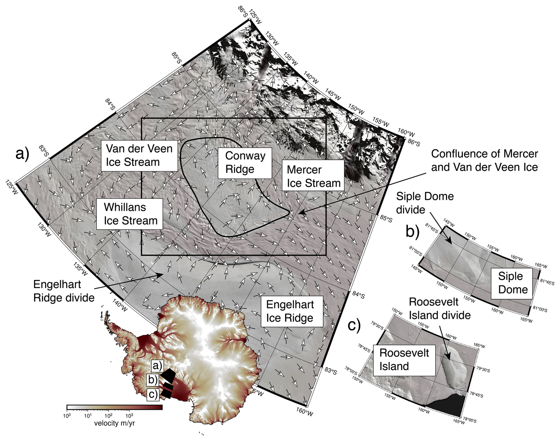
Figure 1 (a) Overview of MODIS image mosaic of Mercer Ice Stream, Conway Ice Ridge, and the van der Veen Ice Stream. Also labeled are (a) Engelhart Ice Ridge, (b) Siple Dome, and (c) Roosevelt Island, which are divides or ice ridges that all have prominent divides (black lines) visible in satellite imagery.

Many of the inter-stream ridges and ice rises located along the Siple and Gould Coasts show signs of stable divides in surface imagery (Siple Dome, Engelhardt Ice Ridge, and Roosevelt Island; Fig. 1). An exception is Conway Ice Ridge located in the western part of the Siple Coast. Unlike Engelhardt Ridge or Siple Dome, Conway Ice Ridge does not have a single divide (Matsuoka et al., 2015). The surface elevation of the ridge slopes relatively steeply toward the grounding line driving flow down the ridge rather than orthogonal to the ridge axis (Joughin et al., 2002; Mouginot et al., 2019). Conway Ice Ridge may also be particularly well suited for understanding ice sheet readvance because it sits at the junction of van der Veen, Whillans, and Mercer Ice Streams. Surveying the englacial structure of Conway Ice Ridge presents an opportunity to link the geologic history of grounding-zone changes recorded in sediment records collected from beneath the ice streams that flow past Conway Ice Ridge with the mechanics and strain history recorded in Conway Ice Ridge englacial stratigraphy.

Here, we interpret detailed ice-penetrating radar surveys collected on Conway Ice Ridge that reveal past ice-flow conditions over the ridge and the adjacent van der Veen and Mercer Ice Streams. We complement these observations with model simulations of the ridge to constrain the physical mechanisms that might have promoted these changes. Together, our observations and model simulations of Conway Ice Ridge suggest that the neighboring van der Veen Ice Stream and the confluence of van der Veen and Mercer Ice Streams were thinner and moved faster before thickening, advancing, and stagnating to their present flow configuration in the last three thousand years. These observations and model simulations of a thinner, faster flowing West Antarctic Ice Sheet in the western Ross Sector complement biogeochemical evidence of ice sheet readvance during the late Holocene.

2 Data and Methods

During field seasons conducted in the austral summers of 2001–2002 and 2003–2004, 47 mass-balance measurements and ice-velocity measurements were recorded across Conway Ice Ridge. Approximately 300 line-kilometers of high-frequency impulse ice-penetrating radar data were also collected each field season (Fig. 2). These ground-based field data complement satellite remote sensing datasets of Conway Ice Ridge collected between 1997 and the present (Fig. 2). We next introduce each data product and describe the methods for processing each dataset.

2.1 Ice-Penetrating Radar Data

Variations in ice thickness and englacial stratigraphy were measured using a custom high-frequency impulse ice-penetrating radar system (Conway et al., 2002). Radar data were collected primarily using antennas with a center frequency of 2 MHz (∼80m wavelength in ice), but multiple lines were also collected with 7 MHz antennas (∼20 m wavelength in ice). The radar survey (Fig. 2) was designed to sample both the along- and across-flow topography as well as features of interest identified in satellite imagery of surface morphology and velocity. Radar data were acquired at a constant distance interval of ∼15 m using an odometer wheel. Relative positions and orientations between radar traces still vary slightly due to traversing over surface features with variable wavelengths, such as windblown snow or sastrugi.

Radar waveforms were stacked 300–500 times per trace, with the number of stacks determined by driving speeds (time taken to traverse 15 m). Where available, dual-frequency GPS data were used to determine the positions and surface elevations of radar traces. If dual-frequency GPS data were not collected contemporaneously with the radar data, horizontal radar trace positions were interpolated linearly between end points of the profiles where dual-frequency GPS positions were recorded. Surface elevations along radar profiles were interpolated from the Reference Elevation Model of Antarctica (REMA; Howat et al., 2019) if dual-frequency GPS data were not collected for that profile. We do not correct for surface elevation change as the integrated effect of these signals are small in the area of the survey compared to the range resolution of the impulse radar system. We confine our surface elevation interpretations from radar data to individual profiles to account for the multi-year temporal offset between the time of collection of GPS data and optical stereo-imagery used to construct REMA.

Radar data were processed following the workflow of Christianson et al. (2016) with some modifications. First, a time correction for antenna spacing was applied to account for transmitter-receiver separation. A bandpass filter between 1–5 or 4–9 MHz was then applied to the 2 and 7 MHz data, respectively. Following geolocation, shorter, spatially adjacent or overlapping profile segments were concatenated to facilitate migration and radar interpretation. Along-track time-wavenumber migration was then applied to more accurately image subsurface reflection positions and slopes. Migration and conversion of travel time to depth assumed an average radar wave speed in ice of 168 m µs⁻¹.

The corrected bed-returned power and depth-averaged and depth-variable englacial attenuation rates for individual traces were calculated for multiple reflectors in each trace (see Appendix A for additional information). Following Taylor et al. (2004) and Bingham and Siegert (2007), we used Fourier spectral analysis to quantify along-track bed topographic roughness (see Appendix B). These methods assume that the reflection coefficients of internal layers are spatially continuous and that the relative reflectivity between layers is constant for the same transmit pulse settings (these settings include amplitude radiation pattern, transmitted power, and refractive focusing). We chose these power correction methods because they do not depend on assumptions for internal layer or bed depth variability or bed reflection power. As explained in Appendix A, the reflectivities results appear inconclusive, and we therefore do not include these findings in the subsequent analysis.

Due to the absence of continuous layers in englacial radiostratigraphy recorded at Conway Ice Ridge that can be traced and dated to an ice core site, we calculate a depth-age relationship to determine the age of the englacial layers we interpret using analytic models of ice sheet vertical velocity (see Appendix C for additional information). We choose to apply two relatively simple depth-age models due to spatiotemporal uncertainty in input parameters (accumulation rate, basal-melt rate, and ice-flow parameters) and vary these parameters over physically plausible ranges to estimate the age of englacial layers. Accumulation rates across the ridge used in these calculations are shown in Fig. C1. These models were chosen with the goal of determining the possible range of ages for our deep and shallow bounding layers, rather than providing a precise depth-age scale for this site.

2.2 Velocity Data

We used velocity data from two sources: in-situ dual-frequency GPS data acquired contemporaneously with the ice-penetrating radar data and satellite SAR imagery. Repeat dual-frequency GPS measurements, acquired at 47 stake locations in November 2001 and November 2003, were used to determine local ice velocity over those two years. Stake positions were determined both seasons using dual-frequency GPS differential carrier phase positioning in a local (east, north, up) coordinate system relative to the base station (King, 2004). Velocity vectors were calculated by transforming local coordinates to geodetic coordinates and then calculating component differences between acquisitions and dividing by the time elapsed between measurements. We also use three SAR velocity mosaics to examine regional ice-velocity changes (Joughin et al., 2002; Scheuchl et al., 2012a, b; Mouginot et al., 2019). These velocity fields were differenced to determine changes in velocity over the last 20 years (Fig. 2). Speed change is consistent between products and in the figures and discussion we show the difference in speed between the Joughin et al. (2002) and Mouginot et al. (2019).

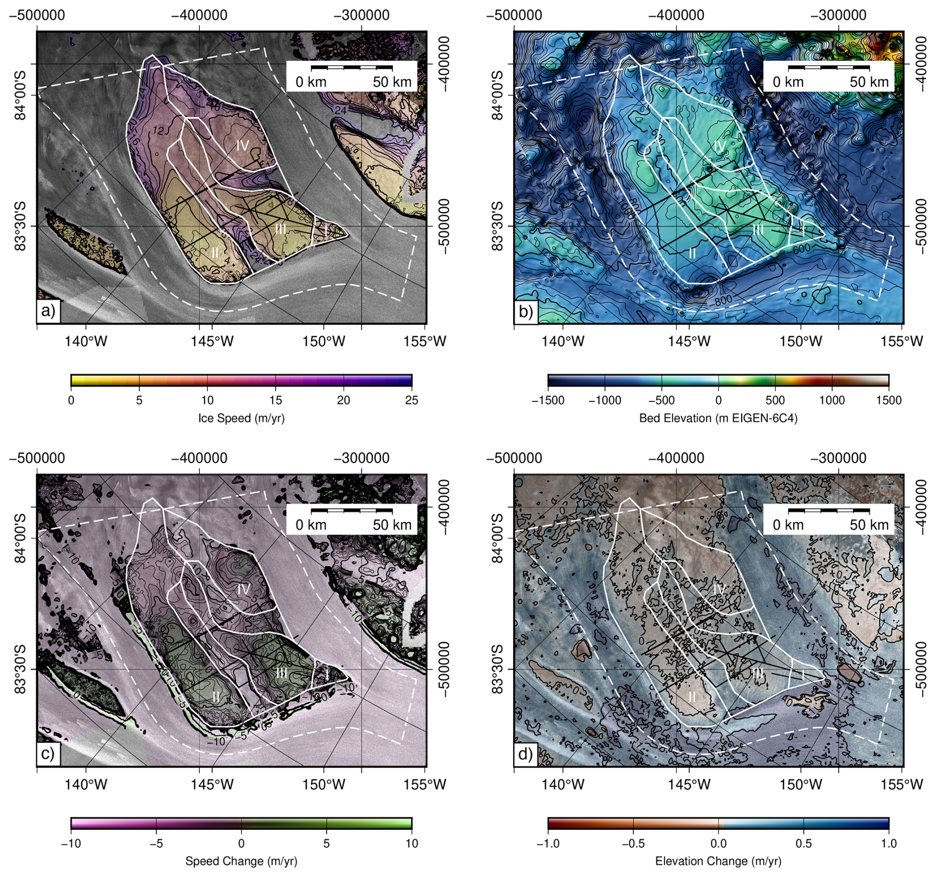
Figure 2 Radar survey interpretation plotted on (a) ice speed (Joughin et al., 2002), (b) bed elevation (Morlighem et al., 2020), (c) speed change from 1997 to 2017 and (d) annual surface elevation change. Radar profiles are plotted in black. White dashed polygon denotes model domain. Solid white polygons denote the four regions of Conway Ice Ridge.

2.3 Elevation Data

The Ice, Cloud and land Elevation Satellite-2 (ICESat-2) has now acquired over five years of surface height data at unprecedented spatial resolution and accuracy (Smith et al., 2019, 2020). We use the recently released Advanced Topographic Laser (ATL) altimeter land-ice products ATL14 (reference elevation) and ATL15 (elevation change relative to reference elevation) (version 1, released 15 December 2021, updated 27 May 2022) to contextualize the changes we observe in surface velocity with changes in elevation observed across Conway Ice Ridge and neighboring van der Veen and Mercer Ice Streams from October 2018 to July 2021 (Smith et al., 2020). We interpolate the reference digital elevation model provided in ATL14 onto the coarser grid for the ATL15 height change time series to produce a time series of elevation change relative to the ATL14 reference digital elevation model. Regional subglacial lakes were masked out of the interpolated elevation change products used in our modeling experiments using elevation change in the area of lake documented by Smith et al. (2009).

2.4 Model Simulations

To understand the mechanisms responsible for evidence of past flow changes interpreted in radar, surface elevation, and surface velocity we use a free-boundary diagnostic ice-flow model (Summers et al., 2023). Our method allows us to solve for both the position of past shear margins and past ice velocity near Conway Ice Ridge associated with past changes in ice thickness, boundary velocity, and basal strength that we prescribe to understand the system's sensitivity to changes in flow velocity and surface elevation. We use this model to understand how different configurations of ice-stream thickness, boundary velocity and basal strength affect flow around Conway Ice Ridge and evaluate mechanisms that can explain our interpretations of the radar data. This diagnostic approach allows us to solve for ice-flow speeds without prescribing accumulation and ocean melt-rate forcing, allowing us to evaluate whether different configurations of ice thickness are consistent with evidence of past fast flow we observe with radar data.

The model developed in Summers et al. (2023) is a thermomechanical ice-flow model based on the free-boundary formulation of ice-stream flow by Schoof (2006) based on shelfy-stream approximations proposed by MacAyeal (1989). We solve a depth-averaged free boundary formation of ice flow over a pure plastic bed using Glen's law rheology with n=3 (see Appendix D for detailed discussion of model assumptions).

$$\begin{array}{}\text{(1)}& \begin{array}{rl}\mathrm{2}{\displaystyle \frac{\partial }{\partial x}}& \left[\mathit{\eta }H\left(\mathrm{2}{\displaystyle \frac{\partial u_x}{\partial x}}+{\displaystyle \frac{\partial u_y}{\partial y}}\right)\right]+{\displaystyle \frac{\partial }{\partial y}}\left[\mathit{\eta }H\left({\displaystyle \frac{\partial u_x}{\partial y}}+{\displaystyle \frac{\partial u_y}{\partial x}}\right)\right]\\ & -{\mathit{\rho }}_{\mathrm{i}}gH{\displaystyle \frac{\partial z_{\mathrm{s}}}{\partial x}}-{\mathit{\tau }}_c{\displaystyle \frac{u_x}{\left|\mathit{u}\right|}}=\mathrm{0},\\ \mathrm{2}{\displaystyle \frac{\partial }{\partial y}}& \left[\mathit{\eta }H\left(\mathrm{2}{\displaystyle \frac{\partial u_y}{\partial y}}+{\displaystyle \frac{\partial u_x}{\partial x}}\right)\right]+{\displaystyle \frac{\partial }{\partial x}}\left[\mathit{\eta }H\left({\displaystyle \frac{\partial u_x}{\partial y}}+{\displaystyle \frac{\partial u_y}{\partial x}}\right)\right]\\ & -{\mathit{\rho }}_{\mathrm{i}}gH{\displaystyle \frac{\partial z_{\mathrm{s}}}{\partial y}}-{\mathit{\tau }}_c{\displaystyle \frac{u_y}{\left|\mathit{u}\right|}}=\mathrm{0},\end{array}\end{array}$$

where u_i is the i component of velocity, ρ_i is the density of ice, g is gravitational acceleration, H is ice thickness, z_s is the surface elevation and τ_c is basal strength, $|\cdot |$ is the L² vector norm and η is the nonlinear viscosity of ice, defined in Eq. (2) of Summers et al. (2023). We include thermal softening by coupling the 1D thermal model of Meyer and Minchew (2018) to solve for the average ice softness at every grid point. Importantly, this approach neglects internal deformation from vertical shear in the ice column. This approximation is reasonable within ice streams and our model can be used to solve for the location of shear margins, but this approximation does not hold well within the ice ridge. Though we show results for the entire domain, model results within the ridge (speeds under ∼30 m yr⁻¹) are likely under estimates of ice speed.

Our model domain is shown in Fig. D1, and discussed further in Appendix D. We select our domain such that the lateral boundaries are defined along modern flowlines in observed surface velocities of the van der Veen and Mercer Ice Streams, and the upstream and downstream boundaries are drawn >10 ice thickness away from our region of interest. Modern surface velocities (Mouginot et al., 2019) were used as boundary conditions along the ice-stream boundaries of the model, upstream and downstream boundaries are stress-free, and modern-day surface and bed elevations define ice thickness throughout the domain (Morlighem et al., 2020). We interpolated the basal strength field from estimates of the basal resistance inferred using the Ice-sheet and Sea-level System Model (ISSM; Seroussi et al., 2019). This basal strength field biases our results towards modern flow configurations, so we intentionally limit our investigation to shear margin migration that is possible without significant reorganization of the basal strength distribution.

Using the model framework described above, we conduct three sets of diagnostic model experiments for Conway Ice Ridge in order to understand the system sensitivity to thinning, acceleration of van der Veen and Mercer Ice Streams, and the basal resistance field as a function of the ice thickness change.

For the thinning experiments, we used the surface elevation change observations derived from ALT14 and ALT15, as discussed in Sect. 2.3, to linearly extrapolate from modern thickness observations to configurations when the ice streams were on average ∼15 m thinner in increments of ∼3 m. We also include one simulation in this experiment where we extrapolate forward in time and prescribe 3 m of thickening.

For the ice-stream velocity experiment, we change the ice-stream boundary velocity conditions relative to modern velocities (Mouginot et al., 2019). We adjust the ice-stream velocities in increments of 10 % from 90 % to 150 % of modern velocities. These perturbations are only enforced at the along-flow boundaries of the domain, allowing the surface velocity structure to change over interior elements in response to changes in overall force balance.

Finally, we evaluate the sensitivity of ice flow around Conway Ice Ridge to assumptions for basal strength, accounting for influences on pore pressure and sliding at the ice-bed interface as the grounding zone advances from the ridge. Much of the bed of Conway Ice Ridge is situated below sea level, and thus, parts of Conway Ice Ridge and the surrounding ice streams are within 100 m of the flotation thickness. When the basal hydrology system is well connected to the ocean, changes in effective pressure on basal sediments vary with the height above flotation, which can change significantly as we force changes in ice thickness. For till-covered grounding zones, basal strength varies linearly with changes in effective pressure (Tulaczyk et al., 2000). We thus run two cases of basal strength dependence on ice thickness: one where basal strength remains independent of ice thickness changes and one where we adjust the basal strength linearly with changes in height above flotation

$$\begin{array}{}\text{(2)}& {\displaystyle }{H}^{\mathrm{AF}}=H+{\displaystyle \frac{{\mathit{\rho }}_{\mathrm{w}}}{{\mathit{\rho }}_{\mathrm{i}}}}{z}_{\mathrm{b}}\text{(3)}& {\displaystyle }{\mathit{\tau }}_c={\mathit{\tau }}_{\mathrm{ISSM}}\left({\displaystyle \frac{H^{\mathrm{AF}}}{H_{\mathrm{0}}^{\mathrm{AF}}}}\right)\end{array}$$

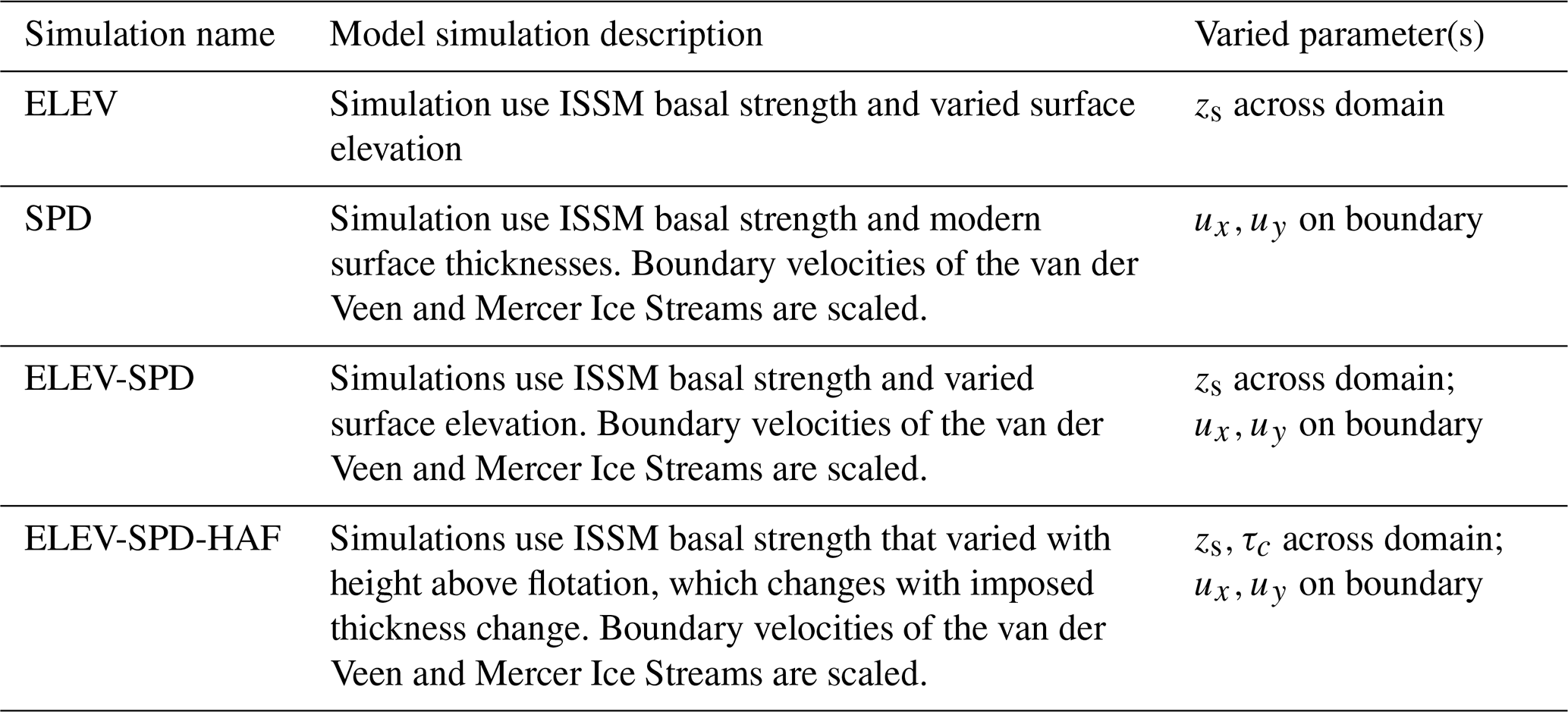
where H^AF is height above flotation, H is ice thickness, z_b is bed elevation, ρ_w,ρ_i are the densities of water and ice, respectively, τ_ISSM is the basal strength inferred using ISSM, and $H_{\mathrm{0}}^{\mathrm{AF}}$ is the currently observed height above flotation. A summary of the model runs can be found in table 1. More information about the model as it was applied in this study is included in Appendix D.

We connect our model results back to observations by interpreting two main features: the onset of fast ice motion where surface velocities exceed 30 m yr⁻¹, which we treat as a proxy for shear-margin location, and locations where surface stresses from horizontal strain are high enough to potentially initiate crevasses. We identify the stress conditions that can initiate surface crevasses using a von Mises stress threshold of 200 kPa, the regional estimate for the Siple Coast by Vaughan (1993), and well within the observed estimates of near-surface tensile strength determined from satellite imagery 90–320 kPa Vaughan (1993); Grinsted et al. (2024); Hoffman et al. (2025). To calculate modeled von Mises stress, we compute the modeled effective strain from our modeled velocities and use Glen's rheology to solve for the von Mises stress, assuming the entire column is pure ice:

$$\begin{array}{}\text{(4)}& {\mathit{\sigma }}_{\mathrm{v}}=\sqrt{\mathrm{3}}{A}^{-\mathrm{1}/n}{\dot{{\mathit{ϵ}}_{\mathrm{E}}}}^{\mathrm{1}/n}\end{array}$$

where n=3. Importantly, we use a rate factor $A=\mathrm{1.2}\times {\mathrm{10}}^{-\mathrm{25}}{\mathrm{s}}^{-\mathrm{1}}{\mathrm{Pa}}^{-\mathrm{3}}$ corresponding to −20 °C (Cuffey and Paterson, 2010) ice, which is approximately the mean annual surface temperature for this region. Our stress estimation does not account for internal heating or frictional heating at the bed, but since we are concerned with near-surface crevassing, it is appropriate to use this cold temperature for near-surface ice in our estimation of potential locations where surface crevassing may occur. Using these two model outputs, shear-margin location and the von Mises stress, we evaluate whether different configurations of the ice thickness, ice-stream velocity, and basal strength are consistent with our interpretations of the radar data.

Table 1 Model experiment description and summary.

3 Results

3.1 Satellite data reveal connections between flow velocity, elevation change, and ridge structure at Conway Ice Ridge

Using the twenty years of satellite observations of surface velocity and elevation in this area, we map recent changes in velocity and ice thickness of Conway Ice Ridge. We calculated ice thickness changes from differences in vertical velocity of the surface from repeat GPS measurements following Hoffman et al. (2020). Vertical velocities from repeat GNSS and accumulation stake measurements over the two-year period indicate that the average rate of thickening for the ridge is +1 cm yr⁻¹. Our result is consistent with previous calculations of the flux divergence using ice thickness measurements and the horizontal surface velocity fields obtained from satellite data that suggest the ridge centers are near balance (Smith et al., 2002). Three-year averages of gridded elevation change observations from ICESat-2 satellite laser altimetry indicate similar rates of thickening (Fig. 2) and coincide spatially with changes in surface velocity (Fig. 2). Where laser altimetry reveals ongoing thickening, the ice velocities have also slowed; where the ice-sheet thickness is unchanged, the flow velocities of the ridge are also unchanged over the last twenty years (Fig. 2).

The distributed horizontal surface velocity and surface elevation fields also reveal the modern structure of Conway Ice Ridge that informed the designation of regions we use to present and discuss our radar and modeling results. Velocities derived from GPS and satellite imagery reveal that Conway Ice Ridge is currently bisected by two regions of faster flow (Fig. 2). These small inter-ridge tributaries drain much of the ice from the interior of the ridge to Mercer Ice Stream and Whillans Ice Stream (Fig. 2). Near the confluence of Mercer and Whillans Ice Streams, there is also a promontory where ice flows slowly from Mercer Ice Stream towards Whillans Ice Stream.

These three features (the inter-ridge regions of faster flow and the promontory where ice flows from Mercer towards Whillans) separate the ridge into four distinct regions that generally coincide with changes in the surface velocity and elevation of the ridge (Fig. 2) and surface roughness revealed in SAR backscatter and passive microwave imagery (Jezek, 1999). We refer to the promontory near the confluence of Whillans and Mercer Ice Streams as region I. Here, ice on the seaward tip of the ridge moves more slowly than the surrounding Mercer and Whillans Ice Streams and a tributary internal to the ridge that transports ice from Mercer to Whillans Ice Stream. On the northeastern ridge immediately adjacent to van der Veen Ice Stream, the surface is smooth in both SAR and MODIS imagery and qualitatively looks similar to the currently inactive Siple Ice Stream (Fig. 1; Jezek, 1999; Jacobel et al., 2000; Catania et al., 2005). We refer to this region as region II. To the west of region II is a small internal tributary that separates region II from the southwestern ridge, which we refer to as region III. In this region, near the confluence of Mercer and Whillans Ice Stream, the surface is generally smooth, but is interrupted by several depressions that run orthogonal to the surface elevation gradient. South of this region is the inter-ridge tributary that flows into Mercer Ice Stream that separates region III from the southern ridge, which we refer to as region IV. Here, the surface of the the ridge is rough, and average flow velocity is higher than any of the other slow flowing regions. These four regions, the promontory near the confluence of Whillans and Mercer Ice Streams (region I), the northeastern ridge (region II), the western ridge (region III), and the southwestern ridge (region IV), are marked in Fig. 2.

3.2 Radar data uncover present-day ridge structure and buried evidence of past ice-stream expansion

Ice thickness varies from 800–1200 m on Conway Ice Ridge (Fig. 2b). The thickest ice is on the northeastern side of the ridge in region II, towards the currently active shear margin of van der Veen Ice Stream, where we image half of a trough that is ∼300 m deeper than the surrounding basal topography (km 60 to km 70 in Fig. 5). The current van der Veen shear-margin position does not coincide with the boundaries of this trough. The interior edge of this trough sits ∼10 km towards the ridge center from the current shear margin.

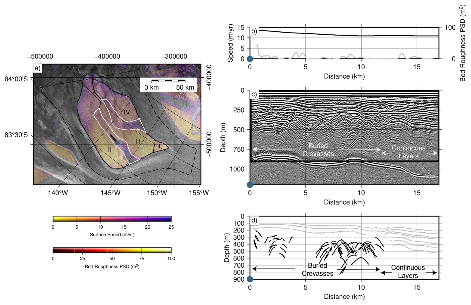
Figure 3 Along-flow radar profile in the central tributary of Conway Ice Ridge. (a) Radar profile location, bed roughness, and speed map plotted on SAR imagery. (b) Ice speed and bed roughness along the profile as a function of distance. (c) Radargram with continuous layers and crevasses labeled. Black box shows limits of radargram portion in panel (d). (e) Interpretation of portion of radargram shown in black box in panel (c). Crevasses are consistent with past faster flow in the first two-thirds (downflow) section of the profile.

The interior tributaries where ice flows rapidly between region II and region III and between region III and region IV are underlain by wide (∼20 km) basal troughs that are ∼300 deeper than the surrounding topography (km 30 to km 50 in Fig. 5). These troughs become shallower as the ice flows downstream into van der Veen and Mercer Ice Streams (Fig. 5). Interior ridge tributaries appear to be unique to Conway Ice Ridge compared to other inter-stream ice-ridges along the Siple coast where the bed topography is smooth outside of the regions of fast streaming flow (Siegert et al., 2004a). Ice surface velocities are faster in these troughs. In the margins of these tributaries and across the promontory, we observe changes in the shorter wavelength bed roughness. In particular, along the profile near the confluence of Mercer and van der Veen Ice Streams (Fig. 4), the transition from slow (<5 m yr⁻¹) to faster (>5 m yr⁻¹) flow speeds are co-located with rougher bed topography (Fig. 4a–c). These rough shorter wavelength features of the bed are also associated with visible depressions in SAR and MODIS surface imagery (Figs. 1, 5).

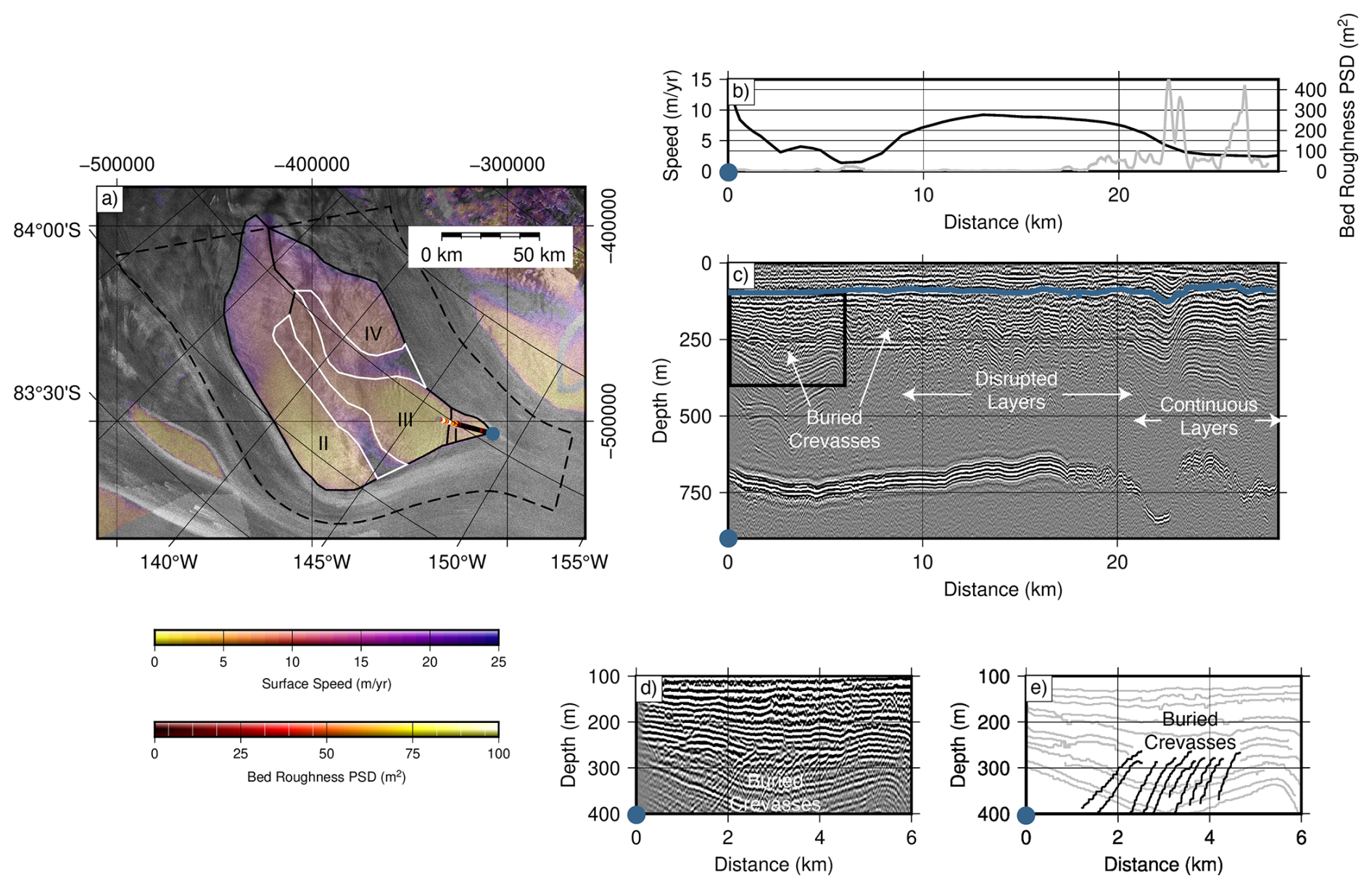
Figure 4 Radar profile at the confluence of van der Veen and Mercer Ice Streams on the western promontory of Conway Ice Ridge. (a) Radar profile location, bed roughness, and speed map plotted on synthetic aperture radar imagery. (b) Ice speed and bed roughness along the profile as a function of distance. (c) Radargram with location of buried crevasses and deepest continuous layer (traced in blue) along the profile with age ∼850 years before present. Areas of crevassing, disrupted layers, and continuous layers are labeled. (d) Close-up radargram showing buried crevasses (black box in panel c). (e) Interpretation of radargram shown in panel d. Internal layers and hyperbolic reflectors indicative of buried crevasses are plotted in gray and black, respectively.

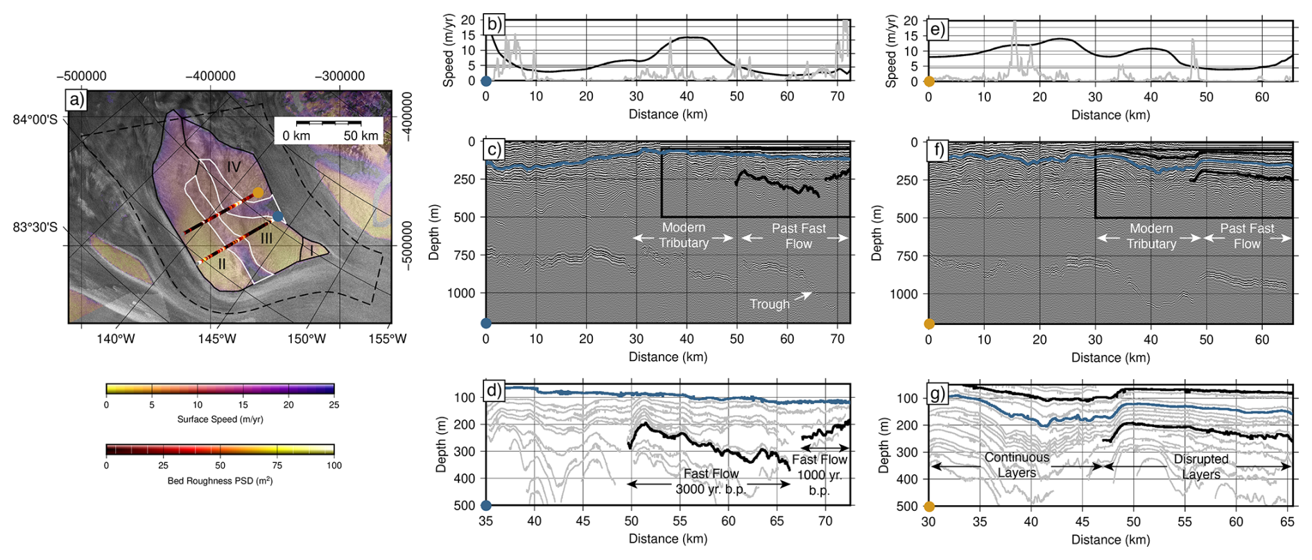
Figure 5 Southern radar profiles across Conway Ice Ridge from Mercer to van der Veen Ice Stream (south to north). (a) Radar profile location, bed roughness, and speed map plotted on SAR imagery. (b) Ice speed and bed roughness along the profile as a function of distance. (c) Radargram with location of deepest continuous layer (∼850 years before present, and shallowest and deepest continuous layers marking time period of recent slow flow on this former tributary of van der Veen Ice Stream. Areas of continuous and disrupted layers are labeled along the profile. Black box shows limits of radargram portion in panel (d). (e) Interpretation of portion of radargram shown in black box in panel (c). From km 50 to the end of the profile, continuous layers between ∼3000 and ∼1000 years age (marked in solid black) are above deeper disrupted layers consistent with faster ice flow.

In profiles that cross slow flowing regions of Conway Ice Ridge (regions III and IV), bed conformal layers are generally present through the entire ice column (e.g. km 0–30 of the profile in Fig. 5c and km 0–30 of Fig. 5f). However, in locations where there is modern fast flow (>5 m yr⁻¹), for instance within the troughs that bisect the ridge (i.e. km 30–50 of profile in Fig. 5c and km 35–45 in Fig. 5f), observed layers are not bed or surface conformal. The abrupt change in layering with depth suggests a change in the strain history of the ice. There are two prominent observations of disrupted stratigraphy where ice flow is currently slow (<5 m yr⁻¹), indicating that stratigraphy may document past, more rapid ice-flow conditions in these locations.

The first observation of disrupted layers occurs on the eastern side of region II, where ice flows from Conway Ice Ridge into van der Veen Ice Stream shown in Fig. 6c km 50–72, Fig. 5f km 50–65. Here, smooth surface conformal stratigraphy is present in the top, younger portion of the ice column, but layers are deformed in the lower, older portion of the column. Following Conway et al. (2002), we determined the timing of the changes in stratigraphy by tracking the deepest undisturbed layer above the disrupted stratigraphy. We then date the disturbed layer using a model for the vertical ice advection through the column and the apparent depth of the feature (Fig. 6 and Appendix E; Nye, 1959; Dansgaard and Johnsen, 1969).

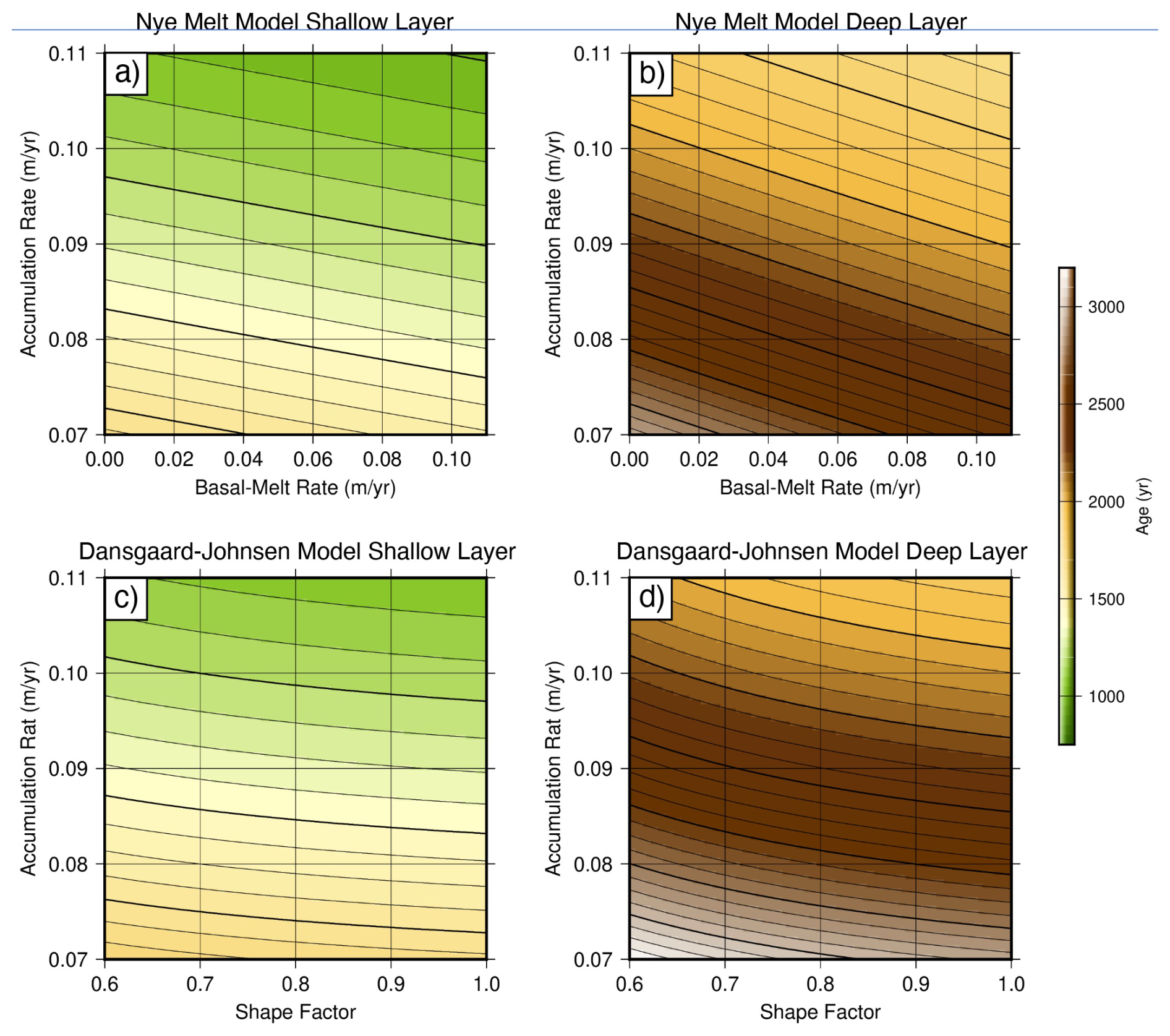
Figure 6 Age fields calculated for the two different feature depths (shallow layer observed at promontory and in the tributary that flows into the van der Veen Ice Stream. These ages were derived using Nye flow model assumptions (a, b) and Dansgaard-Johnson flow model assumptions (c, d) for the vertical advection of ice according to prescribed surface accumulation and basal melt and assumptions for internal shear in the ice column.

Our results indicate that layers deposited in the last 1000 years are continuous and surface conformal, whereas layers deposited between ∼1000 and ∼3250 years before present are disrupted so that they are not surface or bed conformal but are generally traceable, and deeper layers older than ∼3250 year before present are only continuous for short intervals and are not easily traceable. These disturbed layers in the upstream profile (km 50–65 in Fig. 5e–g) are consistent with past streaming flow and suggest the van der Veen margin migrated northward (narrowing). In the more downstream profiles, the same signal of outward migration of the margin (km 50–65 in Fig. 5b–d) suggests the ice stream also narrowed downstream; however, the disturbed layering ∼10 km closest to the present day margin is shallower suggesting it slowed later (∼1500 to 950 years before present). The shallower, and thus younger, disturbances closer to the margin in downstream profiles indicate that the stagnation and shear-margin migration started from upstream and that the van der Veen shear margin migrated northward 3250 years before present by 36 km prior to migrating another ∼10 km to the current position at a slower rate ∼1000 years before present.

The second observation of disrupted layering is in region I and in the interior of the fast-flowing tributary separating regions II and III. In these locations, hyperbolic reflectors at depth are consistent with the presence of buried crevasses (Fig. 4c–e; Clarke et al., 2000; Conway et al., 2002; Catania et al., 2006). At the northwestern tip of the promontory (region I), stratigraphy is disturbed below 100 m depth and smooth and surface conformal above 100 m depth (younger than ∼750 years before present) on the seaward 20 km of the profile (Fig. 4). More than 20 km inland from the confluence tip in region I, stratigraphy is smooth and bed conformal throughout the full ice column. The strong direct radar wave arrival prevents interpretation of stratigraphy in the upper ∼100 m of the ice column, so our ability to comment on changes in the recent past (∼400 years) is limited in the interior regions of the ridge.

In the tributary between region II and region III crevasses are imaged at 200–300 m depths (Fig. 3). Using continuous layers traced above these hyperbolic reflectors, the presence of buried crevasses across the survey indicates that the surface stresses were previously sufficiently high to promote surface fracture (Vaughan, 1993; Colgan et al., 2016; Hoffman et al., 2025). In the area of the tributary between regions II and III, depth-age calculations (see Appendix C) suggest that the buried crevasses would have been exposed at the surface ∼3000 years before present or earlier in this region. The abrupt transition between continuous, surface conformal layers at shallower depths (<300 m) and buried crevasse features suggest that ice flow slowed rather abruptly ∼3000 years ago. The smooth stratigraphy to the shallowest observable depths suggests that flow has remained relatively slow through the tributary to the present. At the tip of the ridge at the confluence of the ice streams, buried crevasses are present at ∼200 m depth below the surface for the first 10–15 km inland from the confluence tip (Fig. 4). These depths correspond to an age of ∼1000–750 years before present, suggesting that ice slowed later here.

3.3 Numerical simulations show that shear-margin location is sensitive to small changes in ice thickness

To better constrain the physical processes that might have led to the ice-dynamic changes suggested by our radar data, we use an ice-flow model to understand how the velocity field at Conway Ice Ridge responds to changes in ice surface elevation, basal strength, and the velocity of the neighboring van der Veen and Mercer Ice Streams. We use this model to identify how ice thickness change, ice-stream velocity change, and changes in basal strength could produce past flow conditions consistent with those inferred from internal stratigraphy. Specifically, we compare our model results against observations of disturbed layering implying historic shear-margin location, and buried crevasses implying historically elevated surface stress conditions.

We show the spatial changes in ice thickness in Figs. 3, D3 derived from ICESat-2 ATL14/15 measurements used to test three different velocity responses to changes in ice thickness and boundary flow conditions. In these cases, we prescribe (i) thinning, (ii) thinning with 1.5× speed up of Mercer and van der Veen Ice Streams, and (iii) thinning, speed up, and weakening of the basal strength field depending on the height above flotation. The surface elevation fields produce the ice speeds shown in Fig. 7 (see Fig. D4 for all model experiments). The black dashed line represents the 30 m yr⁻¹ contour, and the gray dashed line is the 30 m yr⁻¹ contour of the present day case plotted for comparison. Figure 7e–g shows the modeled surface stress, with a green dotted line and the abrupt change from blue to green in color scale corresponds to 200 kPa, the von Mises threshold we associated with surface crevasse formation.

We find that across most of the domain the shear margin defined by the 30 m yr⁻¹ contour remains stable in response to changes in thinning, with the notable exception of the promontory region. Here, our simulations show significant migration of the Mercer and van der Veen Shear Margins in response to ∼6 m of prescribed thinning (Fig. D4). In these cases where we consider only changes in ice thickness, we do not detect notable change in the location of the 200 kPa surface stress contour, which is our proxy for likely crevasse formation. This is true even for the case when we prescribe 15 m of thinning (Figs. 7b–d, D4).

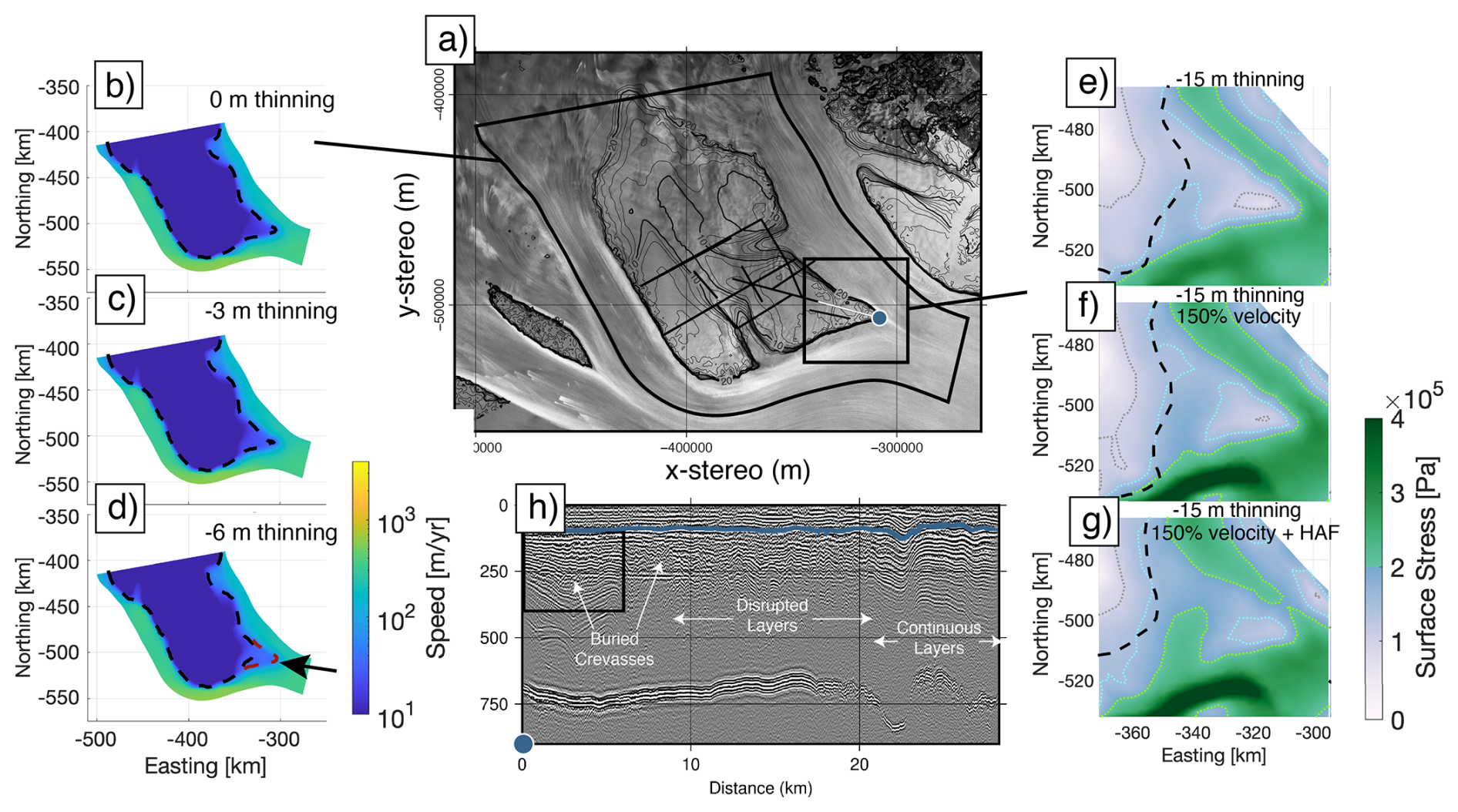
Figure 7 Model summary figure showing (a) the simulation domain with radar lines. Contours of observed surface speed are included, with major contours at 10, 20, 30 m yr⁻¹. (b–d) the resulting velocity field associated with prescribed thinning experiments in increments of 3 m of thinning (in the area of the ice streams). Also shown are the surface von Mises stress shown as a function of boundary forcing and assumptions for basal strength weakening for the Conway Ice Ridge Promontory (e–g). (h) Radar profile highlighting buried crevasses and disturbed layering observed along the promontory.

To consider the impact of changing regional ice velocities on Conway Ice Ridge, we alter our boundary conditions to mimic a change in the ice-stream velocities that bound the ice ridge. We find that changes to ice-stream velocity do not impact shear-margin location as much as changes in surface height, but do impact the surface shear stresses near shear margins and across the promontory, as shown in Fig. D5. Though speed up of the ice streams does increase surface stresses, stresses across the promontory remain below 200 kPa our proxy for likely crevasse formation (Fig. 7f).

Finally, to consider the impact of changing basal strength with changing overburden pressure, we consider the scenarios above, but with basal strength now varying as a function of changes in height above flotation (HAF). This basal strength scenario considers the case of a perfect connection between the subglacial network and the ocean, resulting in a linear relation between basal strength and height above flotation. Compared to the cases where we hold the basal strength constant, the HAF dependent basal strength scenarios exhibit more migration at the promontory shear margin, as well as higher surface stresses at the promontory shear margin for all the prescribed thinning cases with increased ice velocity (Figs. 7g, D7). The cases of 130 %–150 % velocity are the only cases that surpass the 200 kPa von Mises stress threshold for crevasses formation in the region of observed buried crevasses.

4 Discussion

Biogeochemical evidence from subglacial sediment cores suggests that a relatively short-lived (<1000 years; Venturelli et al., 2020; Neuhaus et al., 2021), but spatially extensive (hundreds of kilometers) phase of grounding-line retreat in the Ross Sector in the early-Holocene (Catania et al., 2006; Spector et al., 2017; Kingslake et al., 2018) may have been followed by a period of ice-sheet readvance in the late-Holocene (Greenwood et al., 2018; Kingslake et al., 2018; Venturelli et al., 2023). These constraints on past grounded ice-sheet extent agree with climate model simulations that suggest late-Holocene changes in submarine ocean-driven melt can drive marine outlet glacier retreat and readvance in the Ross Sector (Lowry et al., 2024). The past ice thickness, flow velocity, and grounding-zone location of the ice sheet during readvance are difficult to constrain with sediment records because the deposits that have been used to date past ice-sheet extent record only the local grounded or ungrounded state of the ice sheet in time (Venturelli et al., 2023). Our radar observations complement these paleo grounding-zone markers by providing the first distributed spatiotemporal indicators of fast flow and crevassing that span Conway Ice Ridge and adjacent areas of Whillans and Mercer Ice Streams.

Disturbances in layering we observe near the promontory (region I) and the northern side of the ridge closest to van der Veen shear margin (region II) are consistent with shear-margin migration and stagnation of Conway Ice Ridge. Our data suggest that these changes occurred in phases. The northern margin of van der Veen Ice Stream began to migrate northward (30 km) rapidly (3000 years before present) before more slowly narrowing to the configuration we observe today (region II). The narrowing occurred just before crevassing stopped at the junction of van der Veen and Mercer Ice Streams (region I). This phased response is consistent with ice-stream readvance, with an older, thinner, faster-flowing ice sheet progressively thickening and stagnating to the configuration we observe today.

From our model results, we can evaluate potential mechanisms responsible for the slowdown. At the promontory, simulated shear-margin position can be explained by thinning of the ice sheet by about 9 m. Our simulations show little additional inland migration when we prescribe additional surface thinning (i.e. the 12 and 15 m thinning experiments). Varying ice-stream velocities results in very little additional change in shear-margin location or surface stresses, but slightly increases surface von Mises stress for high velocity scenarios; however, these surface von Mises stresses remain well below ∼200 kPa.

For experiments where we assume a linear relation between height above flotation and basal strength, there is minimal additional change in shear-margin position, but surface stresses increase markedly. Surface stresses in region I exceed 150 kPa and occasionally exceed 200 kPa in scenarios where ice-stream velocity is also increased (1.5× of the modern velocity). These changes in shear-margin position and surface stress near region I in response to prescribed thinning and weakening match or exceed the inland extent of disturbed layering and relic crevasses we observe in radar data at the promontory. The agreement between our model and radar results suggest that basal strength may also change as the ice ridge and ice streams thin to flotation. Taken together, our radar interpretations and model results suggest that flow over Conway Ice Ridge is sensitive to the configuration of the West Antarctic Ice Sheet, accelerating as ice streams widen in response to grounding zone retreat and stagnating as the grounding zone readvances (Fig. 8).

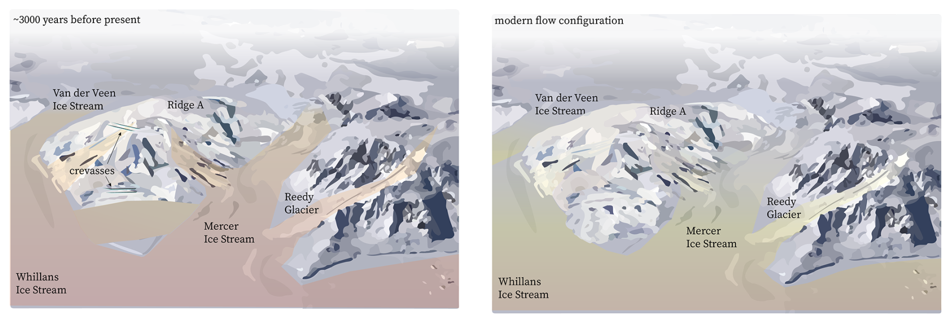
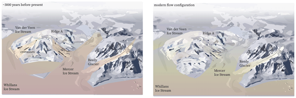
Figure 8 Schematic of the past flow configuration of Conway Ice Ridge as viewed from the Ross ice shelf looking South. Darker red colors in the schematic indicate faster flow compared to yellow colors. Approximately 3 kyr BP the ice streams around Conway Ice Ridge flowed faster and were thinner than present. This flow is recorded in buried crevasses that we see in the tributary that flows into van der Veen Ice Stream and across the promontory.

We note that our model simulations do not reproduce changes in width or migration of the northern van der Veen Shear Margin. The prescribed changes in elevation are small (<15 m) and decrease inland along the van der Veen Shear Margin. This suggests that the ice sheet was thinner in the interior than the prescribed ice thickness change field we use to evaluate shear-margin sensitivity, or that basal strength field has changed in this region in response to factors not dictated by height above flotation alone . Although there is some modern thinning in the interior of the ridge, there is zero prescribed elevation change in the areas where our radar data indicate past shear-margin migration of the northern van der Veen Ice Stream (Figs. 2d, 3, D3). Van der Veen shear margin would have had to thin substantially in order to reach a height above flotation similar to the promontory, where weakened basal strength strongly affects shear-margin migration and surface stress in our model experiments. Alternatively, a change in the flow network of the subglacial hydrologic network could have impacted the basal strength in this region without requiring major changes in ice sheet thickness (Elsworth and Suckale, 2016).

There are a few caveats in radar interpretation and model implementation that are relevant to interpreting results. The first is our approach to dating stratigraphy, which rely on 1D ice-flow models that are often applied to ice cores, where accumulation rate history, basal-melt rate and shape factor can be verified or constrained with measurements. Although we explore dating sensitivity to these parameters, layer date uncertainty is still hundreds of years, and was used to create a qualitative chronology. The second potential weakness is the connection between our prescribed thinning fields and historical years. The thickness fields we use in our model were derived from modern rates of surface elevation change and therefore include temporal information in addition to spatial thinning information. Recent limited observations of surface elevation change for this region show an acceleration in thickening (Nilsson et al., 2022), which points to a clear mismatch between historical thinning and thickness change prescribed assuming a fixed thickening rate from a modern reference state. If we were to assign modern thickening rates for the 750–1000 years to estimate the elevation when we estimate buried crevasses and disrupted layering formed at the surface, the entire promontory and much of the presently grounded Mercer and van der Veen Ice Streams would have ungrounded. However, radiocarbon data and recalculation of cosmogenic exposure age data from Reedy Glacier near its confluence with Mercer Ice Stream indicate thinning began 3 kyr BP and reached present-day elevations by ∼2.4 kyr BP (Hall et al., 2013). The third major consideration is the surface stress threshold associated with crevassing, which is subject to large uncertainty (Vaughan, 1993; Grinsted et al., 2024; Hoffman et al., 2025). Cold surface temperatures may also infiltrate in regions of crevassing, stiffening ice, and resulting in higher surface stresses for a given strain, which would effectively lower the tensile strength of the near surface ice and produce fractures at lower von Mises stresses.

Although our data do not allow a precise chronology, the radar data and model results we present indicate a progressive slowdown of Conway Ice Ridge that proceeded from south to north in the late Holocene that is consistent with progressive thickening of the van der Veen Ice Stream. Our model results suggest that thickening in connection to strengthening of the bed led to narrowing of the van der Veen Shear Margin and stagnation across Conway Ice Ridge. These results are generally consistent with biogeochemical evidence of a late-Holocene readvance of Whillans and Mercer Ice Streams. In the mid-Holocene (∼7.2 kyr BP), the Whillans Grounding Zone retreated well past its current location (Venturelli et al., 2020). Radiocarbon dating of subglacial sediments and sediment porewater chemistry collected at Subglacial Lake Whillans suggest that grounding zone retreat continued inland until ∼4.5 kyr BP, before subsequently ice-sheet readvance over Subglacial Lake Whillans ∼1.1 kyr BP (Neuhaus et al., 2021). The phases of ice thickness change and stagnation recorded in radar stratigraphy on Conway Ice Ridge are contemporaneous with these biogeochemical markers. Readvance and local thickening initiated on Conway Ice Ridge by about 3000 years before present and the ridge stabilized to its current ice-flow configuration about 1000 years ago. These results suggest that the eastern and northern sides of Conway Ice Ridge are sensitive to the dynamics of nearby Whillans Ice Stream and are the first geophysical evidence that bolster the late-Holocene readvance that has been proposed by interpreting subglacial sediment records. Our results also suggest that the western side of Conway Ice Ridge appears less sensitive to these changes. This is consistent with more muted phases of stagnation and grounding-zone readvance for Mercer Ice Stream, which would be consistent with radiocarbon and cosmogenic data from the confluence of Reedy Glacier and Mercer Ice Stream that do not record thickening in the late-Holocene (Todd et al., 2010; Hall et al., 2016; Spector et al., 2017).

5 Conclusions

Conway Ice Ridge has long been considered the least stable of the Ross inter-ice stream ridges due to the rough surface morphology and ice flow through the ridge (Matsuoka et al., 2015). Our ice-penetrating radar, velocity, and elevation data provide new insights into past changes in ice flow through this ridge. On the northern side of the ridge (region II), smooth surface-conformal stratigraphy overlying disrupted stratigraphy indicate a narrowing of van der Veen Ice Stream and slowing in region II between 3000 and 1000 years before present. Our data also suggest that the ridge readvanced seaward of the promontory (region I) and slowed during the same time period that van der Veen Ice Stream narrowed, migrating northward. We are unable to precisely constrain the timescale for shear-margin migration on the northern side of the ridge, but changes in margin position appear to have occurred faster than the vertical resolution of the radar, which suggests a relatively rapid reorganization in less than 250 years.

Along with guidance on the past ice-flow history of the Ross Sector, our data-informed modeling provides physical support for how regional changes in ice thickness, velocity and basal strength impact shear-margin evolution and regional grounding-zone advance (and retreat). We simulate the most recent lateral migration of the shear margin at the confluence of the Mercer and van der Veen Ice Streams, in the context of late-Holocene ice-stream readvance (Venturelli et al., 2020; Neuhaus et al., 2021) and the conditions that produced significant crevassing at the current ridge promontory. These model experiments suggest that the features we observe in radar data are consistent with ice-stream thickening and strengthening of the ridge that has stagnated following a phase of faster flow through thinner ice streams. The phenomenological character of these changes are consistent with late-Holocene ice-stream readvance hypotheses (Venturelli et al., 2020). Future studies in other locations should use radar stratigraphy to inform thermomechanical modeling that may further constrain the geometry of the late-Holocene grounding-zone response of the West Antarctic Ice Sheet to external forcing.

Appendix A: Radar Attenuation and Corrected Bed-Returned Power

We cannot directly measure ice temperature, fabric, or damage using impulse radar data. We can calculate attenuation rates, which are linked to ice temperature, englacial chemistry, and the englacial reflector geometry. We empirically correct returned power for spherical spreading and englacial attenuation to calculate corrected bed-returned power. Following many other authors (Bogorodsky et al., 1985; Winebrenner et al., 2003; Jacobel et al., 2009; Matsuoka et al., 2012; MacGregor et al., 2015; Christianson et al., 2016), we use a simplified form of the radar power equation to describe the radar returned power in terms of its constitutive components:

$$\begin{array}{}\text{(A1)}& P_{\mathrm{r}}=P_{\mathrm{t}}{\displaystyle \frac{A^{\mathrm{2}}Rq}{\mathrm{4}\mathit{\pi }(\mathrm{2}z{)}^{\mathrm{2}}B}}{e}^{-\mathrm{2}\mathit{\alpha }z}\end{array}$$

where P_r is the power recorded at the receiver antenna, P_t is the transmitted power, A is the antenna gain, R is the power reflection coefficient, q is refractive focusing, z is the one-way travel path to the reflector of interest, B is birefringence losses, α is the dielectric absorption coefficient (attenuation coefficient), and 4π(2z)² is spherical spreading (which assumes the target is large relative to the first Fresnel zone). If we assume the source and near surface terms (refractive focusing) do not vary spatially, we can group them as one source term S=P_tA²q. Then, if we correct the returned power for spherical spreading, P_c=P_r4π(2z)², neglect birefringence losses for which corrections require polarimetric radar data unavailable for this site (Fujita et al., 2006; Matsuoka et al., 2009), and log-transform the equation (decibels, [dB]), we have:

$$\begin{array}{}\text{(A2)}& \left[P_{\mathrm{c}}\right]=\left[S\right]+\left[R\right]-\mathrm{2}Nz\end{array}$$

where for each variable in equation A2, $\left[X\right]=\mathrm{10}{\log }_{\mathrm{10}}\left(X\right),$ and N=α(10log ₁₀(e)) is the one-way attenuation rate in dB km⁻¹ (Winebrenner et al., 2003).

Following Eq. (A2), we can use linear regression to determine the englacial attenuation rate if we correct the returned power for spherical spreading, assume that the source terms do not vary, and assume that each reflector has a power reflection coefficient R this is not spatially variable and that reflectivity does not vary between reflectors. Here, we conduct two regressions. First, we fit all reflectors within a moving depth-constrained vertical windows (100 m) that does not span the entire ice thickness. This results in depth-variable (or interval) attenuation rate. Second, we extract the bright reflectors (reflectors with P_c in the top 10 % of all received data in a moving depth-constrained vertical window, again 100 m) throughout the entire ice column and calculate the attenuation rate using a single linear regression through the full ice thickness (Matsuoka et al., 2010). We choose bright reflectors here because they are more likely to be representative of true dielectric constants in the ice, especially deeper in the column where signal-to-noise ratio is low (Matsuoka et al., 2010). For both methods, we define the full thickness as ∼100 m below the surface to 85 % of the ice thickness to avoid the direct arrival and low signal-to-noise deep in the ice column.

Radar attenuation results are difficult to interpret because they may include processes that reduce the amplitude of the radar wave that are not associated with radar attenuation, including destructive interference and backscatter from steeply sloping layers that does is not incident upon the receiving antenna. For these data, trends in attenuation rates are not constant between the two field seasons, suggesting that they may be related to data quality and confounding issues listed above rather than physical properties, such as ice temperature or chemistry. During the 2001–2002 field season, radar data were collected using low-frequency 2 MHz antennas. These data yield low-attenuation rates that may be the result of low signal-to-noise ratios in the radar data. Radar quality, especially deeper layer resolution, are substantially improved in the 2003–2004 field season when 7 MHz antennas were used compared to earlier data, so we focus interpretation on these data. Despite these improvements, many signals in the data are related to bright layer packets, layer slopes, and lack of signal due to deformed layers. Thus, we are hesitant to interpret attenuation results as indicative of ice temperature variability. We are similarly hesitant to interpret corrected bed power because it relies on accurate determination of attenuation. For data collected in the 2003–2004 field season, attenuation rates appear to be higher on the north side of the ridge and lower on south side. This result is mainly due to more disrupted layers on the north side of the ridge, which is consistent with more recent rapid flow on this portion of the ridge. We applied attenuation rate and geometric spreading corrections to bed returned power, but did not find patterns in the data that could be separated from attenuation rates signals, which we do not interpret for the same reasons we are hesitant to interpret attenuation rates.

Appendix B: Bed Roughness

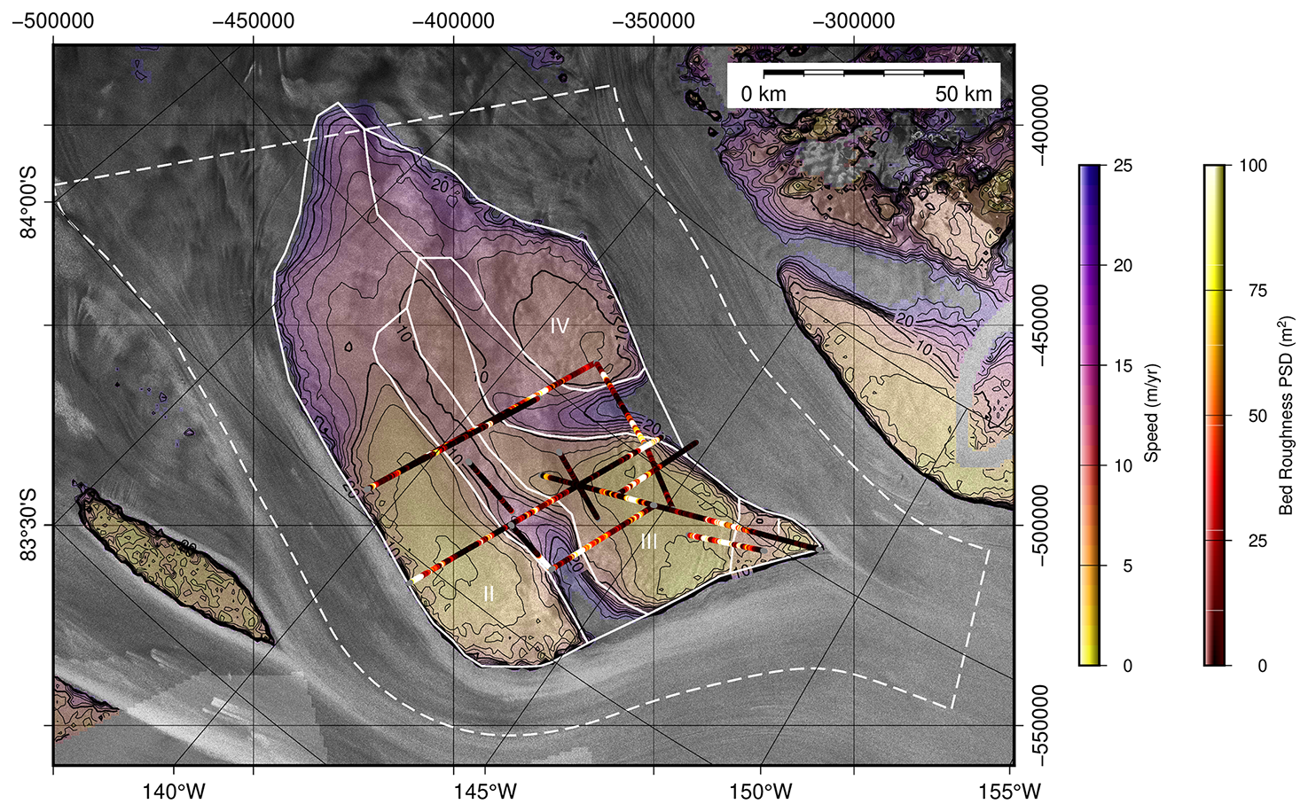
Figure B1 Map of sum of power spectral density across all wavelengths in 1000 m moving window for the entire Conway Ice Ridge radar survey plotted over SAR velocity data (Joughin et al., 2002) and RADARSAT-1 SAR imagery (Jezek et al., 2013; Jezek, 1999). Velocity contours (black) are plotted with a 2 m yr⁻¹ interval. Velocities above 25 m yr⁻¹ and grounding lines are masked in the velocity field.

We use a discrete Fourier transform to determine the spectral power associated bed topography as a function of wavelength. Specifically, we calculate the discrete Fourier periodogram to determine the power associated with each constituent wavelength of topography:

$$\begin{array}{}\text{(B1)}& P\left(k_x\right)={\displaystyle \frac{\mathrm{1}}{N_x^{\mathrm{2}}}}\left|Z\right(k_x){|}^{\mathrm{2}}\end{array}$$

where

$$\begin{array}{}\text{(B2)}& Z\left(k_x\right)=\sum _{n=\mathrm{0}}^{N_x-\mathrm{1}}z\left(n\mathrm{\Delta }x\right)e^{-\mathrm{2}\mathit{\pi }i\frac{k_{x}n}{N_x}}\end{array}$$

Z(k_x) is the discrete Fourier transform of a data set z(x), in this case depth to the bed, x is along-track distance, n is an index in z, and the transform has N_x evenly sampled nodes in frequency space at wavenumbers (spatial frequencies) k_x. Our processing follows the workflow of Booth et al. (2009) for spectral analysis of high resolution topographic data. It is similar to other bed roughness implementations in glaciology (Taylor et al., 2004; Bingham and Siegert, 2007), but our workflow uses different window sizes, more high-resolved bed data, and can be organically extended to multiple dimensions. We use the sum of the periodogram over all wavenumbers to represent the total energy associated with bed roughness at the center of each moving window. We note that we can also filter the energy by wavelength to sample frequency bands by only summing periodogram components for a subset of wavenumbers. We apply this discrete Fourier transform in a moving 1000 m window. We first detrend the data, apply a Hann window to minimize spectral leakage, set the DC-component to be zero to account for any offsets due to applying the Hann window, and then scale the output periodogram so that the sum of the periodogram equals the variance of the detrended windowed elevation sample to correct for any reduction in variance caused by the windowing. This results in a spatially-distributed map of the total bed roughness power, which we plot at the center coordinates for each of the moving windows in every radar profile (Figs. 2b, B1).

Appendix C: Dating Stratigraphic Features in Radar Data

We use two models to date stratigraphic feautres in radar data. The first model is the “Nye-melt” (Nye, 1963; Haefeli, 1963; Fahnestock et al., 2001; MacGregor et al., 2016), which assumes a constant vertical strain rate $\dot{{\mathit{ϵ}}_{z}z}$ that is a function of accumulation rate $\dot{b}$, basal-melt rate $\dot{m}$, and ice thickness H:

$$\begin{array}{}\text{(C1)}& \dot{\mathit{ϵ}}={\displaystyle \frac{\dot{b}-\dot{m}}{H}}\end{array}$$

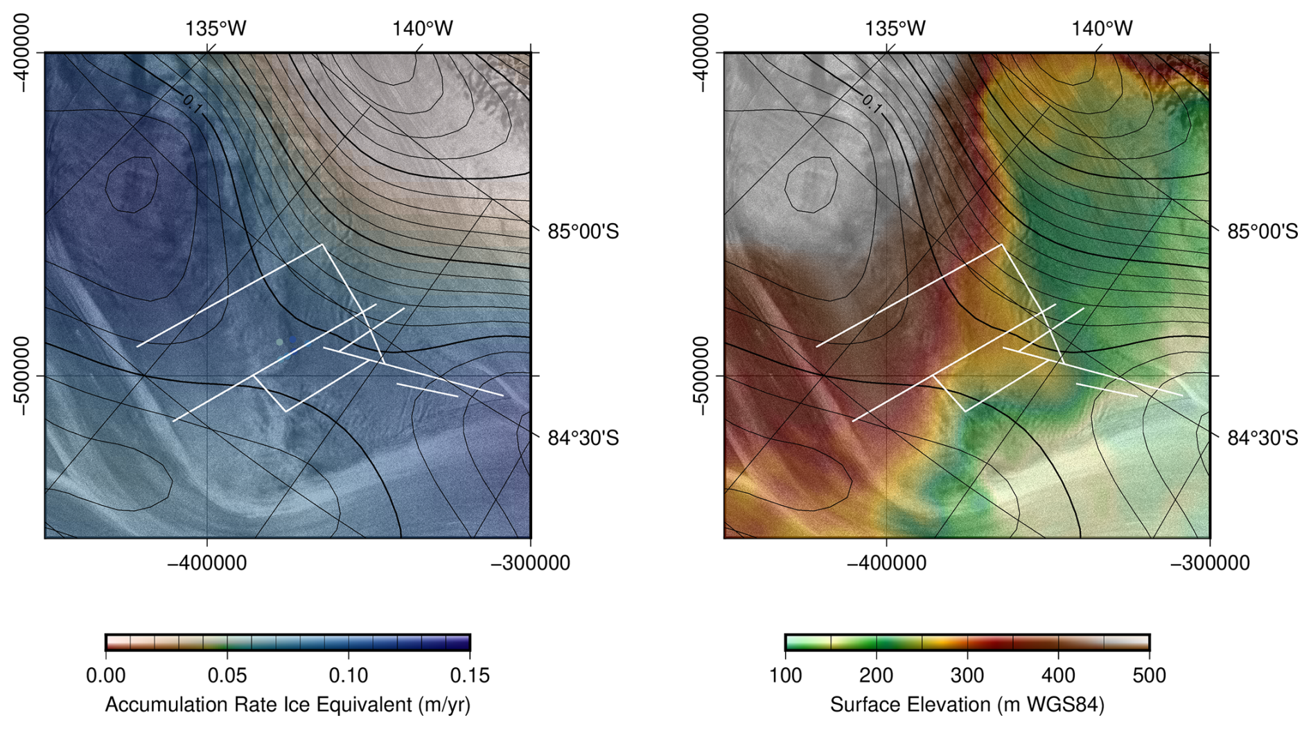
Figure C1 Accumulation rate and surface elevation over Conway Ice Ridge. Accumulation rate patterns across Conway Ice Ridge were used as input to calculate depth-age profiles from models for vertical flow. The surface elevation over Conway Ice Ridge shows that Mercer Ice Stream is steeper than van der Veen and Whillans Ice Stream.

If we integrate an initial layer thickness to a present layer thickness assuming this strain rate and then sum the layer thicknesses of the overlying younger ice, we obtain the following depth-age relationship (MacGregor et al., 2016) of age, Ψ as a function of depth z:

$$\begin{array}{}\text{(C2)}& \mathrm{\Psi }\left(z\right)={\displaystyle \frac{H}{\dot{m}-\dot{b}}}\left({\displaystyle \frac{H-z}{H}}\left(\mathrm{1}-{\displaystyle \frac{\dot{m}}{\dot{b}}}\right)+{\displaystyle \frac{\dot{m}}{\dot{b}}}\right)\end{array}$$

We vary the accumulation rate and basal-melt rate to determine the sensitivity of layer ages to parameter uncertainty. Accumulation rates were varied between 0.7 to 0.11 m yr⁻¹ (ice equivalent), which corresponds to the variability in accumulation rate across the ridge. We vary basal-melt rates between 0 and 0.11 m yr⁻¹. We do not see steep spatially localized synclines that affect all internal layers or any other signs of very high basal melting in the stratigraphy (Catania et al., 2010), so we assume that the highest accumulation rate observed is a reasonable upper bound for highest possible basal-melt rate. Age values were calculated for mean depths and ice thicknesses of two layers between line kilometers 50 and 65 along the profile plotted Fig. 5. Possible ages for the shallow and deep layers vary between 950 and 1690 and 1600 and 2980 years, respectively.

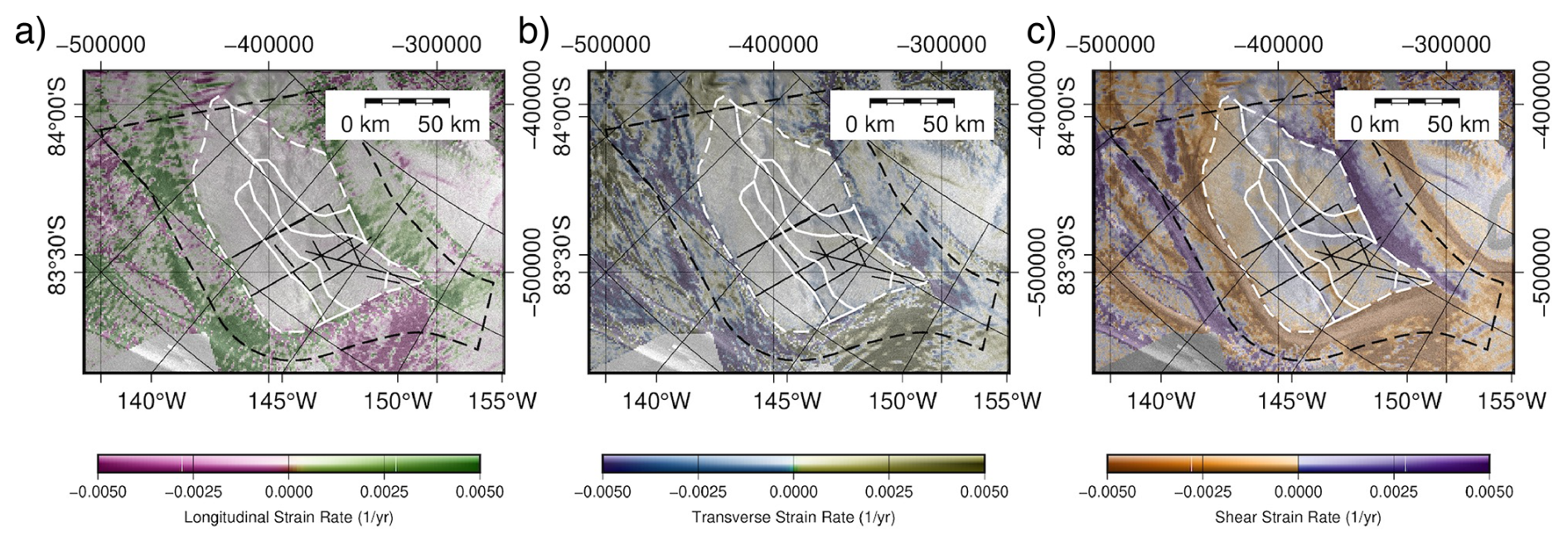
Figure C2 Analytic calculations of strain rates using velocity fields of (Joughin et al., 2002). a) Longitundinal, b) shear, and c) transverse strain rates plotted over RADARSAT-1 SAR mosaic (Jezek, 1999; Jezek et al., 2013). Vectors are the velocity field form (Joughin et al., 2002). Black lines indicate locations or radar profiles and white dots mark locations of GPS stakes.

The second model accounts for a depth-variable horizontal ice velocity by assuming that strain rate is constant to some depth above the base of the ice and then linearly decreases to zero at the ice base (Dansgaard and Johnsen, 1969). Following these assumptions, the depth-age scale is:

$$\begin{array}{}\text{(C3)}& {\displaystyle }\mathrm{\Psi }\left(z\right)={\displaystyle \frac{\mathrm{2}H-h}{\mathrm{2}\dot{b}}}\ln {\displaystyle \frac{\mathrm{2}H-h}{z-h}}\text{ for }H\ge z\ge h\text{(C4)}& {\displaystyle }\mathrm{\Psi }\left(h\right)={\displaystyle \frac{\mathrm{2}H-h}{\mathrm{2}\dot{b}}}\ln {\displaystyle \frac{\mathrm{2}H-h}{h}}\text{ for }z=h\text{(C5)}& {\displaystyle }\mathrm{\Psi }\left(z\right)={\mathrm{\Psi }}_h+{\displaystyle \frac{\mathrm{2}H-h}{\dot{b}}}\ln hz-\mathrm{1}\text{ for }H\ge z\ge h\end{array}$$

where h is the thickness of the basal shear layer and z is height above the ice base. Since we do not have information to constrain the basal shear layer thickness, we assess the sensitivity of ice age to a range of basal shear layer thickness. To determine the range of basal shear layer thickness that is plausible, we calculate the basal shear layer thickness that corresponding to a range of ice-flow shape factors ϕ, which is defined as the ratio between the depth-averaged horizontal ice speed $\overline{u}$ and horizontal ice speed at the surface u_s:

$$\begin{array}{}\text{(C6)}& \mathit{\varphi }={\displaystyle \frac{\overline{u}}{u_s}}\end{array}$$

and shape factor is geometrically related to basal shear layer thickness by:

$$\begin{array}{}\text{(C7)}& \mathit{\varphi }=\mathrm{1}-{\displaystyle \frac{h}{\mathrm{2}H}}\end{array}$$

(Cuffey and Paterson, 2010; MacGregor et al., 2016). If shear stress is assumed the dominant mechanism of ice deformation, the shape factor can be calculated as a function by integrating Glen's flow law, which yields $\mathit{\varphi }=\frac{n+\mathrm{1}}{n+\mathrm{2}}$, where n is the exponent in Glen’s flow law. Although n=3 is the most common assumption which would correspond to a lower bound of ϕ=0.8 and a basal shear layer thickness of h=0.4H, here we take a slight more permissive approach to allow for a range of flow law exponents and ice rheology and allow basal shear layer thickness between zero (activation of basal sliding for which this model becomes no longer physically valid) and h=0.8H. We note that a basal flow law exponent of n=4 would correspond to a basal shear layer thickness of h=0.5H. We vary accumulation rates across the same range of values as earlier (0.7 to 0.11 m yr⁻¹ ice equivalent). For these parameters, this model yields ages for the shallow and deep layers vary between 1020 and 1770 and 1800 and 3250 years, respectively.

Although values are somewhat qualitative for ages, these calculations allow us to broadly consider the plausible range of ages for these layers. The shallow layer ages range between 950 and 1770 years, and we consider 1350±450 years before present a reasonable age range for this layer. The deeper layer ages range between 1600 and 3250 years, and we consider 2400±850 years before present a reasonable age range for this layer.

C1 Strain Rates

We calculated strain rates following the standardized implementation of Alley et al. (2018). This work applies the definition of the surface strain rate tensor given by Nye (1959) and the rotation to the local flow direction from Bindschadler et al. (1996). Input for the strain rate calculations was the Cartesian velocity fields in a polar stereographic projection (EPSG:3031) provided by Joughin et al. (2002). Strain rates in the local flow direction (longitudinal, shear, and transverse) are plotted in Fig. C2.

Appendix D: Model Details

All of the simulations presented in the main text are steady-state solutions that solve for the velocity associated with different assumptions for the ice thickness, boundary velocity, and basal strength. These simulations do not solve a mass balance equation for ice surface response to changes in net divergence of ice velocities and surface mass balance. Instead, the thinning fields and boundary conditions are inputs for our ice flow model which solves for the ice velocities and shear margin position. We use these model outputs to help interpret observations of crevassing and internal layer disruption that we see expressed in radar data. This approach removes the need to resolve stresses outside of the domain and removes any dependence on climate forcing. These assumptions limit the application of our model to simulations when feedbacks from velocity on changes in surface height can be ignored (i.e. periods near the present where observations are available).

We solve for ice velocity by solving the variational form, which reduces the problem to a convex minimization using the Disciplined Convex Programming software package (Grant and Boyd, 2014). This method is detailed in Summers et al. (2023) Sect. 2.3. Parameter fitting of basal strength to best fit observed surface velocities, like the best matching uniform strength bed, was done using a linear-log misfit function, as Eq. (14) of Summers et al. (2023). We use the matlab function fminunc to minimize this misfit, and run our presented models on the best fitting match between model and observed velocities for observed surface height and forcing velocities. This tuned basal strength held constant across all model runs, except for the HAF adjustment detailed in Eq. (3).

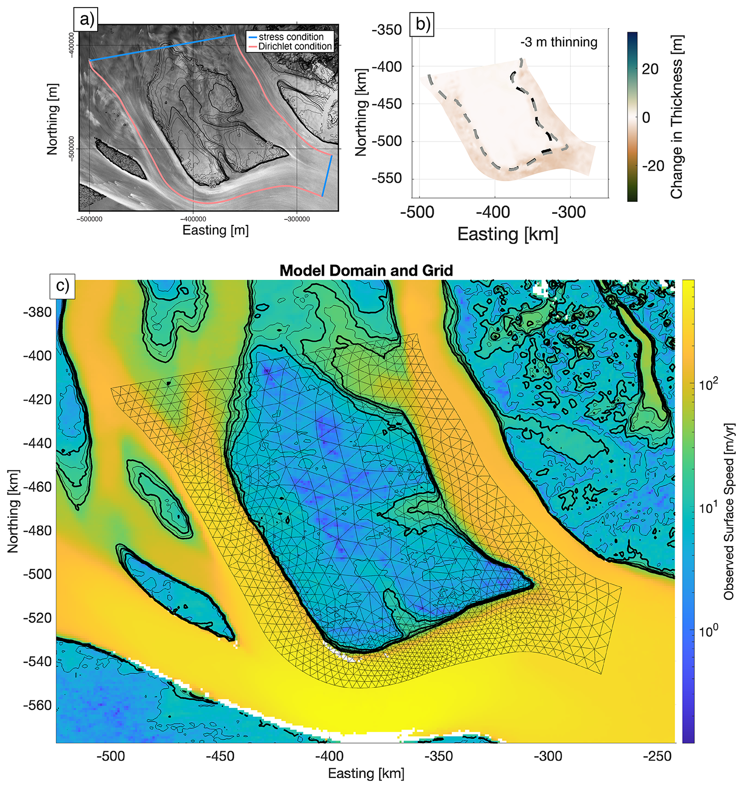
Figure D1 Overview of model domain boundary conditions with (b) the −3 m thickness perturbation field used in thinning experiments. The velocity perturbation experiment changed the velocity condition applied at the Dirichlet boundaries where ice flows approximately parallel to the model domain shown in panel (c). Contours of ice speed are plotted for 5–30 m yr⁻¹ at 5 m yr⁻¹ intervals, bold at 10, 20, 30 m yr⁻¹. Grid resolution is improved near and around regions of increased strain.

We define our domain (Fig. D1) by calculating streamlines in Mercer and van der Veen Ice Streams using Matlab's streamline method, and defining up and downstream cutoff points >10 ice thicknesses away from our region of interest. These flowlines were chosen as lateral model boundaries to allow direct forcing of the velocity of the bounding ice streams.

We use a single triangular grid across all our model runs, using distmesh2d (Persson and Strang, 2004). We first initialize the domain with a uniform triangular mesh, calculate effective strain rates on this grid using observed surface velocities (Mouginot et al., 2019), then creates a refined grid where scale resolution is increased in regions of increased strain. This method produces high resolution in shear margin zones, while saving computational expense with lower resolutions in regions of lower strain.

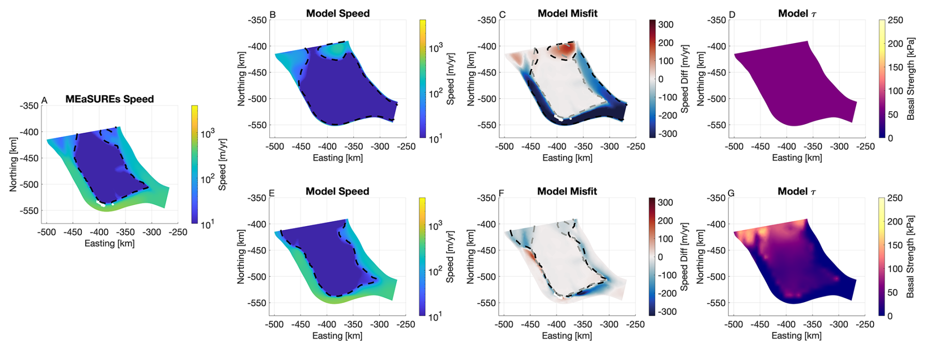
Figure D2 Model speeds compared to MEaSUREs observed ice speeds, as well as the basal strength distribution. (A) MEaSUREs ice speed, (B) Uniform basal strength ice speed, (C) Uniform basal strength residual speed, (D) Basal strength map for uniform basal strength case. (E) ISSM basal strength ice speed, (F) ISSM residual speed, (G) Basal strength map for ISSM basal strength case.

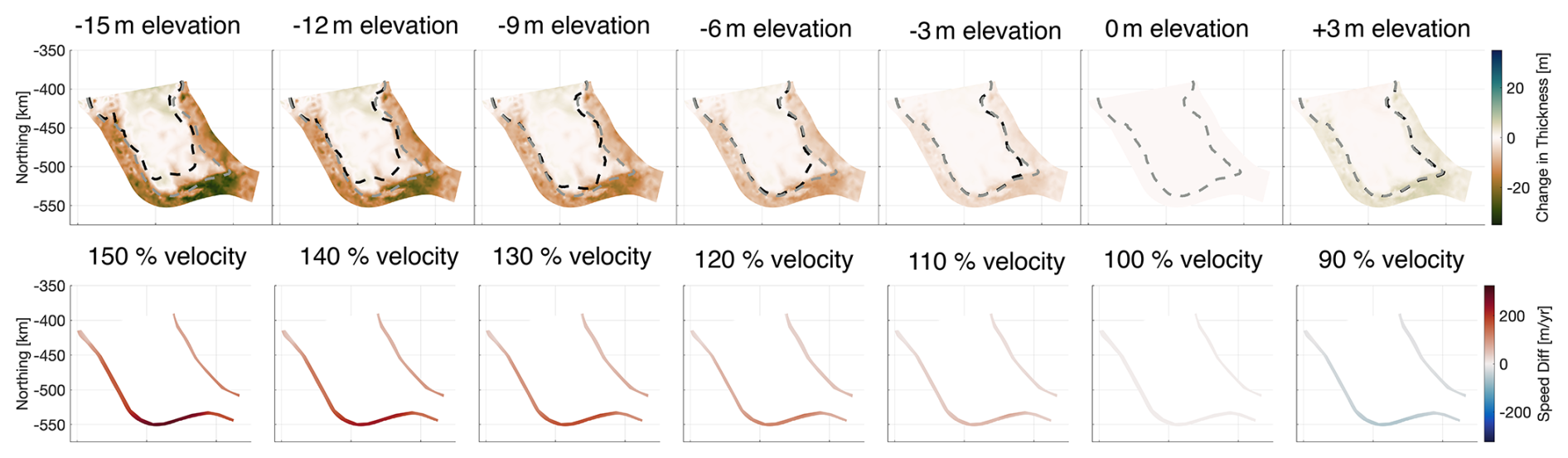
Figure D3 Model velocity boundary conditions used in velocity perturbation experiment and elevation change perturbations in thickness sensitivity experiments. Black lines in elevation perturbation experiment show changes in height above flotation relative no change in height above flotation.

The modeled ice speed and the misfit to ice speed observations with spatially uniform assumptions for the basal strength and basal strengths imported from ISSM simulations are shown for the Conway Ice Ridge in Fig. D2, and reveal that material properties of the ice stream bed control the spatial location of the ice streams neighboring Conway Ice Ridge. The spatially uniform bed strength produces a very poor fit to observed ice velocities, while the spatially variable, ISSM based basal strength provides a much better fit to observations. In particular, for the case where we assume a spatially variable basal strength, the locations of the shear margins and the limits of present day effective surface stresses are in good agreement with current observations of streaming ice and stable ice ridges, particularly in the region around the promontory on the grid south-east corner of Conway Ice Rise. The imported ISSM basal strength reasonably reproduces the current day ice velocities (Fig. D2) and therefore is the basal strength we consider in our main experiments and discussion.

We plot the full range of modeled thinning in Fig. D4, but for thinning beyond −6 m (i.e. −9, −12, −15 m) our simulations show very little additional migration of shear margins on northern Conway Ice Ridge compared to the migration driven by −6 m of thinning. Additionally, for positive changes in ice thickness (+3 to +15 m) results are very similar to the +3 m case, and so are not plotted.

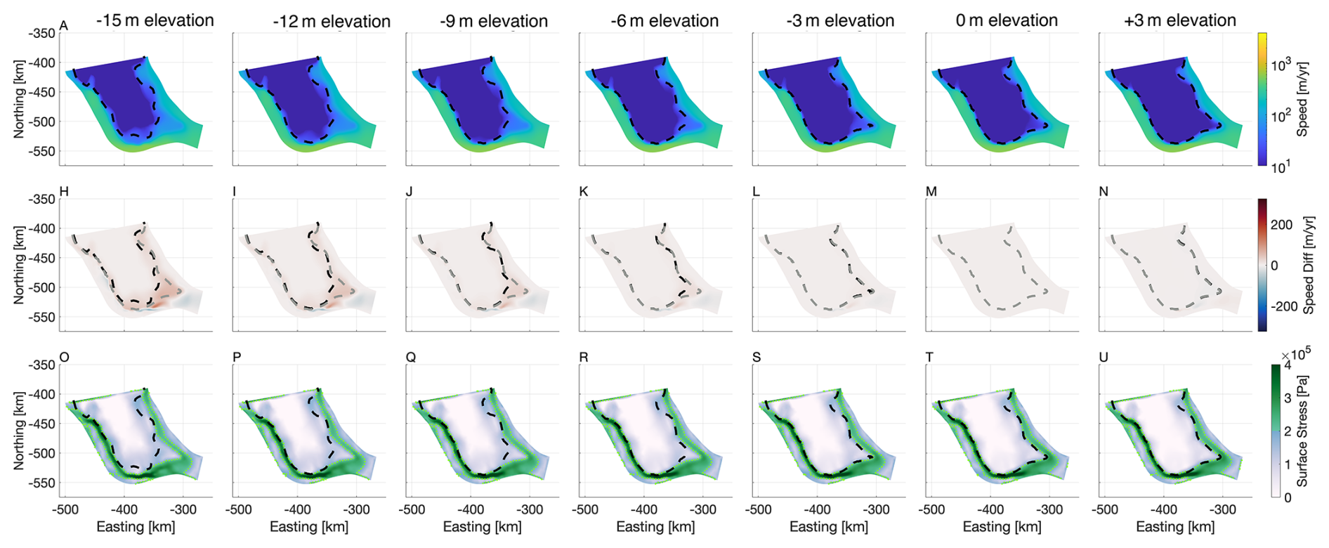
Figure D4 Modeled speed (A–G), Speed difference from control case (H–N), and surface stresses (O–U) for the ISSM basal strength for thickness scenarios −15 through +3 m (ELEV experiments). (M) is the defined control case for all speed difference plots (H–N). Black dashed lines plots the shear margin location in every plot, with a gray dashed line plotting the shear margin location for the control case. The control shear margin location is plotted in all frames to visualize shear margin migration. (O–U) Modeled surface stress, with a green dotted line and abrupt change from blue to green in color scale at 200 kPa.

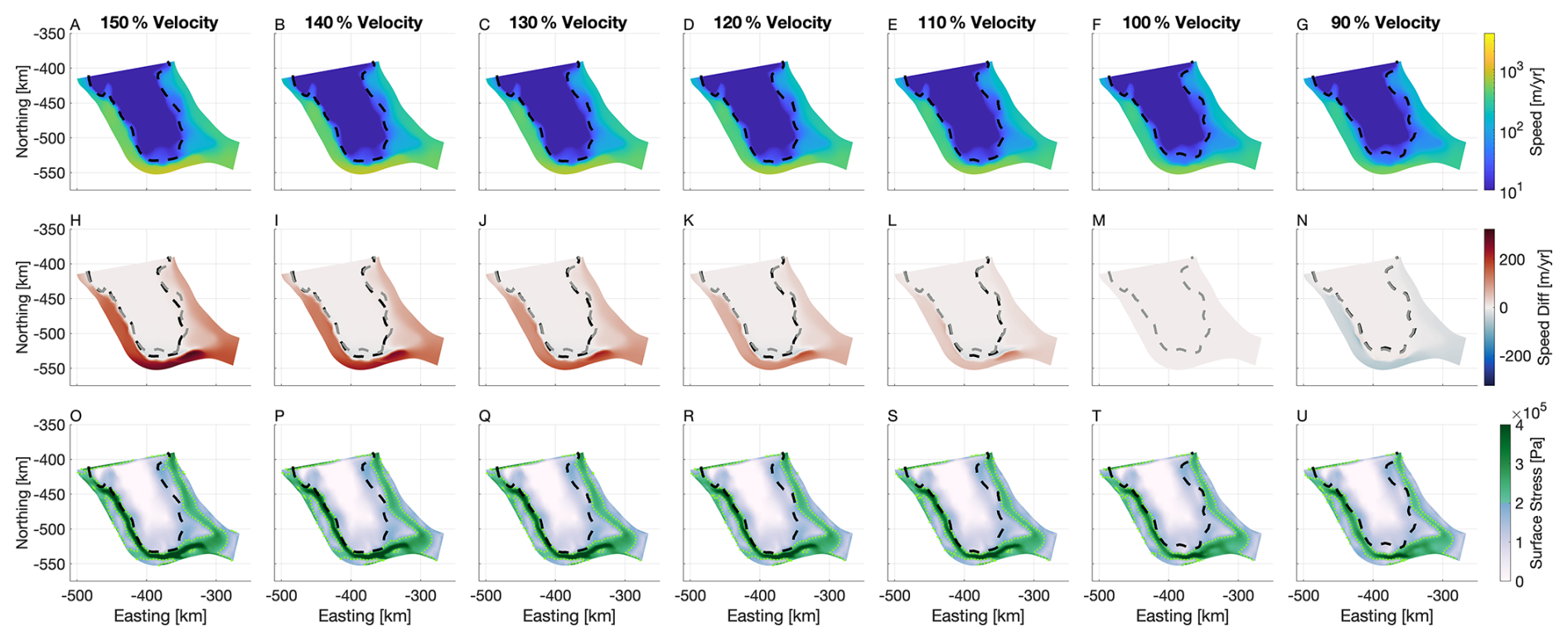
Figure D5 Modeled speed (A–G), Speed difference from control case (H–N), and surface stresses (O–U) for the ISSM basal strength and −15 m ice thickness for ice stream velocity scenarios 150 % through 90 % (ELEV-SPD experiment). (M) is the defined control case for all speed difference plots (H–N). Black dashed lines plots the shear margin location in every plot, with a gray dashed line plotting the shear margin location for the control case. The control shear margin location is plotted in all frames to visualize shear margin migration. (O–U) Modeled surface stress, with a green dotted line and abrupt change from blue to green in color scale at 200 kPa.

Considering changes in bounding ice stream velocity, we take current day observations of the ice velocity at the boundary, and scale them by −50 % to +50 % at increments of 10 %. This enforces a proportional speed-up or slow-down of the bounding ice streams. Our experiments for ice thinning at all values of regional ice velocity produces 121 cases. We focus our attention on the 150 %–90 % speed scenarios, and select the −15 m prescribed thinning cases in Fig. D5. These velocity and thickness assumptions represent perturbations consistent with modern observations of regional change and allow us to interrogate how recent thickness and upstream and downstream flow changes affect local flow without using a mass balance model that requires assumptions for uncertain climate forcing (i.e. regional accumulation, ocean melt).

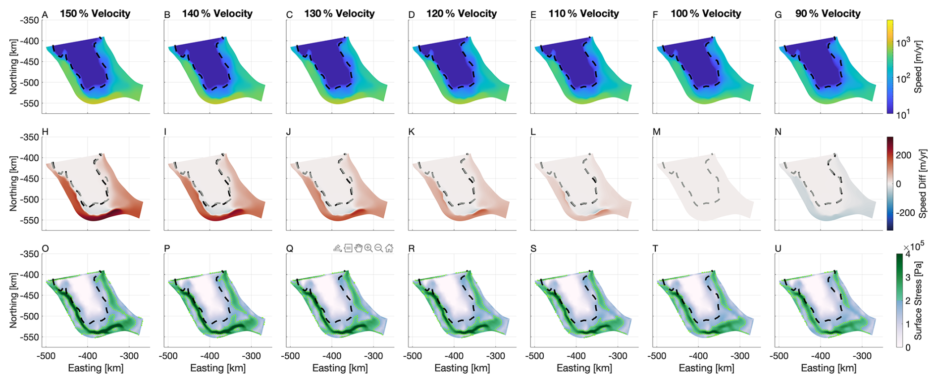
Figure D6 Modeled speed (A–G), Speed difference from control case (H–N), and surface stresses (O–U) for the ISSM basal strength with height above flotation adjustment and −15 m ice thickness for ice stream velocity scenarios 150 % through 90 % (ELEV-SPD-HAF experiment). (M) is the defined control case for all speed difference plots (H–N). Black dashed lines plots the shear margin location in every plot, with a gray dashed line plotting the shear margin location for the control case. The control shear margin location is plotted in all frames to visualize shear margin migration. (O–U) Modeled surface stress, with a green dotted line and abrupt change from blue to green in color scale at 200 kPa.

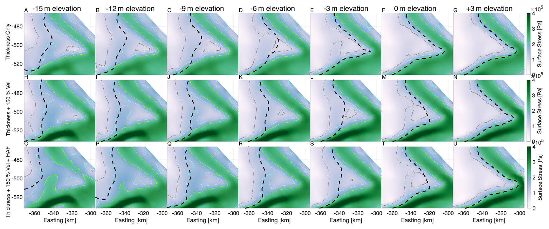
Figure D7 Modeled surface stress near the promontory across numerous modeled scenarios. The colorbar is identical to Fig. D5O–U, with added dotted contours for stress values of 100, 150 kPa in gray and blue respectively. Black dashed line is the 30 m yr⁻¹ modeled speed contour.

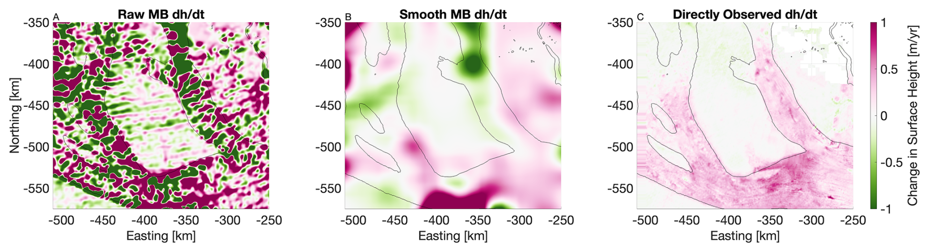
Figure D8 Comparison of our mass balance based estimate of surface height change. (A) Raw estimate of surface height change. (B) The smoothed data product. (C) Directly observed changes surface height.

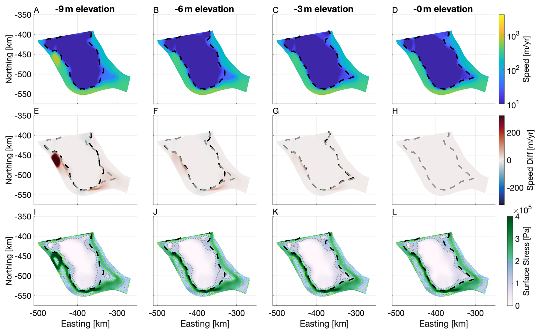
Figure D9 Modeled speed (A–D), Speed difference from control case (E–H), and surface stresses (I–L) for the ISSM basal strength and mass malance based distribution of surface elevation change. (H) is the base case for difference plots (E–G). Black dashed lines plots the shear margin location in every plot, with a gray dashed line plotting the shear margin location for the control case. The control shear mar- gin location is plotted in all frames to visualize shear margin migration. (I–L) Modeled surface stress, with a green dotted line and abrupt change from blue to green in color scale at 200 kPa.

We find that for ELEV-SPD scenarios, changes in bounding ice stream velocity modify flow speed and the shear margin location, moving the South East Ridge shear margin slightly east into the ice ridge. Of note, the shear margin on the North Ridge of the ice rise has the exact opposite behavior, and ice stream speed-up associated with the regional thickening moves the margin further north. The West Ridge shear margin stays stable for all thickness change and velocity change scenarios. The surface stresses at the South West Ridge shear margin however do significantly rise with increasing ice stream velocity, and large areas of over 150 kPa are across this region in the fastest scenario, though these values do remain just below 200 kPa. Though we do not show the impact of changing ice stream velocity on all thinning cases, the overall trend of increasing surface stress with increasing ice stream speed, and relatively little impact on shear margin location is consistent across these cases.

Finally, to consider changing basal strength with changing overburden pressure, we vary basal strength with changes in height above flotation (HAF). Compared to the thickness invariant, ISSM based basal strength cases, the HAF basal strength scenario sees more recent migration of the promontory shear margin, as well as more significant shear margin migration the south-west corner of Conway Ice Rise as shown in Fig. D6. Additionally, the HAF basal strength scenarios results in higher surface stresses at the promontory shear margin for all the prescribed thinning cases with increased ice velocity. The cases of 1.3× to 1.5× speed up are the only cases we consider that surpass the 200 kPa threshold for likely crevasses formation in the region of observed buried crevasses (Fig. D7).

To assess the sensitivity of our model results to the spatial distribution of surface elevation change, we use an alternative forcing approach based on mass balance estimates rather than observed elevation changes. We use satellite observations of surface velocity (Mouginot et al., 2019), estimates of bed elevation (Morlighem et al., 2020) and regional estimates of accumulation (Le Brocq et al., 2010) to solve for the surface height change consistent with Conway Ridge mass balance:

$$\begin{array}{}\text{(D1)}& {\displaystyle \frac{\mathrm{d}H}{\mathrm{d}t}}=-\mathrm{\nabla }\cdot \left({\mathit{u}}_{\mathrm{s}}H\right)+\dot{a}\end{array}$$

where u_s is the vector surface velocity. This derived product is inherently noisy, so we apply a 12.5 km Gaussian filter to smooth the input field for surface elevation change. However, we note that this filtered product still exhibits greater spatial variability than directly observed elevation changes (Fig. D8). Using this mass balance-constrained surface elevation field, we re-run our −9 through −3 m model experiments (Fig. D9). While the distribution of velocity change within the domain differs from our previous results, our key finding – shear margin migration occurring at approximately −6 m of ice stream thinning – remains the same. This suggests that although ice stream flow is sensitive to different realizations of surface height change and corresponding variations in driving stress, the modeled shear margin migration at the promontory remains consistent across reasonably constrained surface height change distributions.