Compounding sub-seasonal variations in Greenland outlet glacier dynamics revealed by high-resolution observations

Understanding the controls on seasonal velocity change for tidewater glaciers may provide insight into long-term retreat and acceleration. Leveraging recent high-resolution satellite data, we examine changes in surface elevation, velocity, and terminus position for four glaciers in Central Western Greenland over 2015–2021. Our approach uses a simplified force balance focused at the terminus to model the expected response in upstream velocity caused by the observed terminus changes. We find that seasonal velocities are strongly controlled by terminus advance/retreat for two glaciers. Residuals between modeled and observed velocities reveal two distinct signals: summertime pulses coincident with peak runoff and wintertime speedup extending several kilometers inland of the terminus. We evaluate the sensitivity of terminus-driven velocity to elevation change by incorporating observed seasonally varying surface topography and applying controlled modifications to the profile, specifically uniform vertical shifts and variations in surface slope. We find surface slope changes impact velocity response to terminus changes more than spatially uniform changes in elevation. Increased surface slope amplifies velocity response to terminus changes. While simplified, our model could be applied to other glaciers to assess the importance of terminus position change as a driver of seasonal velocity.

1 Introduction

The Greenland Ice Sheet (GrIS) is currently the largest land ice contributor to present-day rising sea level (IPCC, 2022) with an acceleration in mass loss over the past few decades in part attributed to ice discharge through outlet glaciers (Shepherd et al., 2012; Enderlin et al., 2014; van den Broeke et al., 2016; The GlaMBIE Team, 2025). This acceleration underscores the importance of comprehending the intricate mechanisms that govern glacier dynamics. Despite the prevalence of glacier acceleration in Greenland, there exists notable spatio-temporal variability in glacier velocity change at a range of time scales (Moon et al., 2012, 2020; Black and Joughin, 2023). This is likely because glacier velocity is influenced by local conditions, like topography, and regionally by environmental factors. For example, runoff and ocean thermal forcing can influence velocity by changing basal friction (Ultee et al., 2022), subaqueous melt rates (Holland et al., 2008), and through terminus fluctuations (Howat et al., 2008; King et al., 2020; Wood et al., 2021).

Outlet glaciers in Greenland present seasonal velocity changes (Moon et al., 2015; Joughin et al., 2008; King et al., 2018), but it is not clear what exact processes are involved. In part, this is because many of the processes that influence outlet glacier velocity are synchronized, making it difficult to disentangle cause and effect. Some studies have suggested increased air temperature leads to summertime melting and terminus retreat, which reduces ice contact with the bed and/or fjord walls and increases net force at the calving cliff, both driving glacier acceleration (Howat et al., 2005; Joughin et al., 2012). Numerical simulations also suggest a non-linear feedback between the rate of terminus change and ice discharge (Sergienko, 2022). Others have indicated that glacier acceleration is due to seasonal changes in basal lubrication related to changes in the subglacial hydrological system (Davison et al., 2020; Stevens et al., 2022; Werder et al., 2013; Andrews et al., 2014), which can cause complex responses in glacier velocities as subglacial conduits grow more efficient (Bartholomew et al., 2010; Andrews et al., 2014; Vijay et al., 2019).

Understanding seasonal drivers of glacier change may help researchers to understand longer term glacier changes. Moreover, numerical simulations suggest that seasonal changes can induce systematic bias in mass loss estimates at the multi-decadal time scale, compared to simulations that do not include seasonal forcing, because the magnitude of mass loss is higher during retreat than mass gain for an equal amount of advance (Felikson et al., 2022; Robel et al., 2018). Thus, investigating the patterns of glacier seasonality may be critical to unveiling the factors that control glacier dynamics into the future.

Previous efforts have classified seasonal velocity variations into types based on the observed timing of velocity change and their correlation to runoff and terminus change (Moon et al., 2014; Vijay et al., 2019, 2021). This classification enhances our understanding of what drives these seasonal variations. Three categories have been generally described in Moon et al. (2014): type-1 has positive correlation of glacier velocity to glacier terminus retreat; type-2 has positive correlation of glacier velocity to summer runoff, and; type-3 shows glacier velocity that slows in late summer and speeds up in winter. As noted in these studies, these velocity patterns connect to multiple underlying processes, and the types are used to describe patterns rather than to assign a single process. In a subsequent study, Vijay et al. (2019) used high temporal resolution velocity data, terminus changes, and radar-backscatter intensity values to classify 45 glaciers into the same three types. Vijay et al. (2021) extended their analysis to 221 glaciers across Greenland, focusing on type-2 and type-3 behaviors. Solgaard et al. (2022) combined velocity and runoff data using a machine-learning approach to classify glaciers throughout Greenland and discussed how subglacial drainage development, runoff volume, ocean interaction, and local conditions can produce similar seasonal patterns. They also noted that multiple processes (e.g., terminus position and runoff) jointly control seasonal flow for many glaciers. Poinar (2023) applied principal component analysis to decompose glacier seasonality in Sermilik Fjord from a statistical perspective, quantifying the prevalence of multiple seasonality types at a single glacier and emphasizing the importance of spatial patterns across the glacier.

These studies have made clear that seasonal velocity patterns are driven by multiple processes. For instance, Moon et al. (2014) reported that some glaciers exhibited multiple velocity types within a single year, and Poinar (2023) explicitly quantified the coexistence of multiple seasonal patterns at individual glaciers. However, these studies were primarily designed to describe dominant or statistically separable patterns. Due in part to the temporal resolution of the data (e.g., monthly or bi-monthly), it has been challenging to resolve the sequential occurrence of multiple processes within a single season. Consequently, the compounding effects of processes that act at sub-seasonal timescales have received less direct attention, especially in physics-based modeling.

Building on the foundation of previous studies, we re-examine glacier seasonality using high-frequency terminus (Zhang et al., 2023), velocity (Gardner et al., 2023), and surface elevation change observations for four glaciers in Greenland. We interpret these observations with an analytical model of velocity response to terminus position change (Joughin et al., 2012). While simple, this model provides a physics-based method to help isolate the myriad processes that influence ice velocity by removing one potential driver, terminus change. By isolating the velocity component driven by terminus changes, we find that glaciers more typically exhibit multiple velocity patterns simultaneously or sequentially within a year. Using high resolution (subweekly) data in this study, we can more accurately decompose these patterns throughout a season, providing a sub-seasonal characterization that may be more appropriate for glacier velocity classification.

2 Study region

We investigate four glaciers in central-west Greenland (Fig. 1): Sermeq Avannarleq (AVA), Sermeq Kujalleq (KUJ), Kangilernata Sermia (KAN), and Eqip Sermia (EQP) over the time period 2015–2021. This time span is specifically chosen to take advantage of the increased sample frequency available in both velocity and terminus position data due to the launch of Sentinel-1/2 in April 2014, which offers full year coverage of velocity data. We choose these 4 glaciers because we want to understand how our simple model might aid interpretation of seasonal velocity change for glaciers that have been extensively studied in the past. These glaciers are selected because they (1) are grounded; (2) exhibit regular seasonal changes in both terminus position and velocity with minimal long-term variations over our study period (Catania et al., 2018; Fried et al., 2018) and; (3) exhibit a range of sub-seasonal behavior in both the terminus and velocity variability. For example, all the four glaciers advance in winter and retreat in summer and yet their seasonal velocity behavior differs over time and space. EQP and KUJ speed up during summertime terminus retreat while AVA and KAN slow down during summertime terminus retreat (Fried et al., 2018). In addition, AVA, KUJ, KAN, and EQP are located close to one another, suggesting that they likely experience the same regional climate forcing. All flowline samples for these glaciers are located within the ablation zone (Noël et al., 2019), implying that meltwater influence is expected across all sampled sites. They also exhibit distinct local effects, such as geometry that impact their dynamic behaviors. For instance, EQP's steep slope results in higher glacier velocities and more frequent calving events (Lüthi et al., 2016; Kneib-Walter et al., 2023), whereas the shallow sills of AVA and KUJ contribute to their remarkable stability over the past century (An et al., 2018).

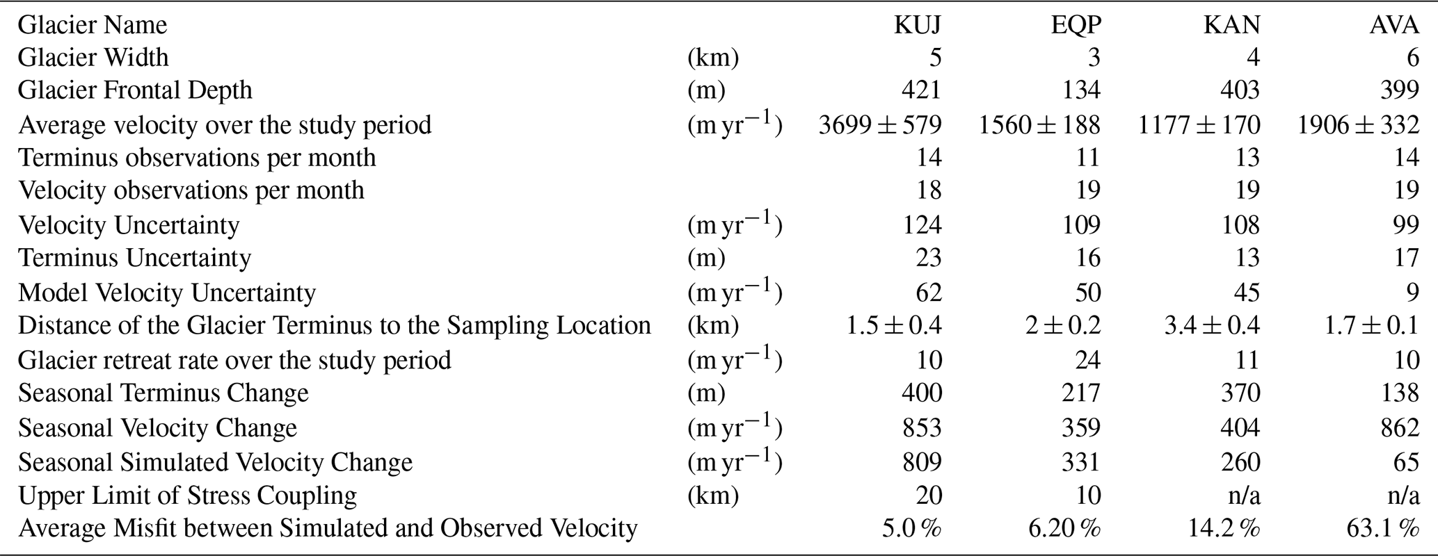
These glaciers have been studied extensively by previous authors. All glaciers have been relatively stable (they have not retreated more than the amplitude of seasonal fluctuations) since 2015 (Table 1). All four glaciers have experienced terminus retreat over the more extensive satellite era; AVA 0.64 km, KUJ 1.80 km, KAN 2.65 km, and EQP 2.54 km from 1999 to 2016 (Catania et al., 2018). Studies of calving style for these glaciers indicate that they all primarily calve via serac failure due to undercutting related to terminus melt (Kneib-Walter et al., 2021; Bézu and Bartholomaus, 2024; Goliber and Catania, 2024), although KUJ has been reported to have a mix of serac failure and buoyant flexure calving styles (Bézu and Bartholomaus, 2024). This suggests that AVA, KAN, and EQP are grounded and that KUJ may approach floatation at times or in smaller regions of the terminus. This is consistent with an earlier study finding that these four glaciers experience terminus change that is predominantly driven by changes in subglacial runoff (Fried et al., 2018). Additional details on each glacier can be found in Table 1.

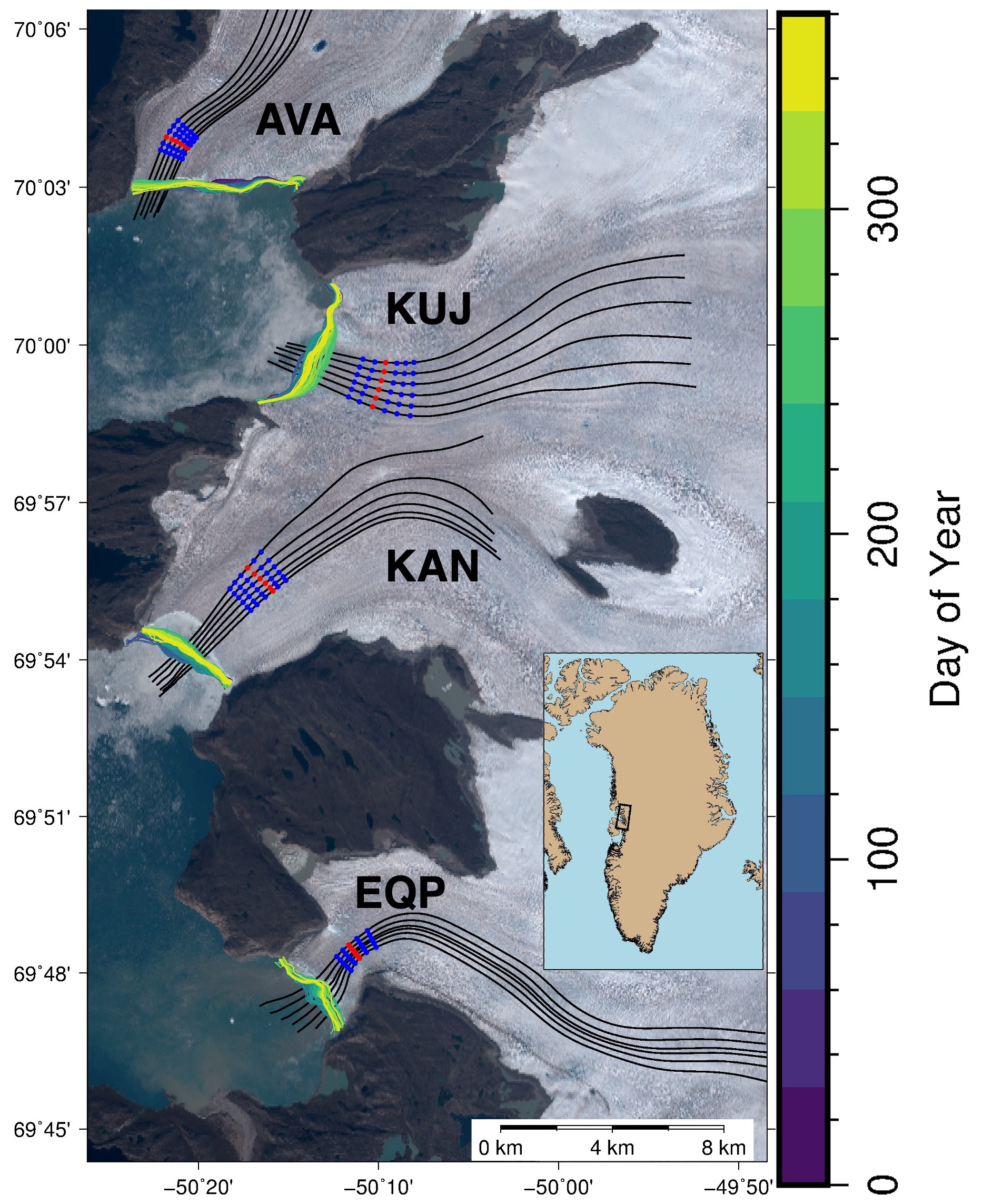
Figure 1 Glacier and data locations. Glaciers examined in this study include Sermeq Avannarleq (AVA), Sermeq Kujalleq (KUJ), Kangilernata Sermia (KAN), and Eqip Sermia (EQP). The terminus traces in 2018 from AutoTerm are colored by day of year. The red points show the locations where ITS_LIVE velocities were extracted for the model comparison in the results section. Blue points are the locations where we tested the sensitivity of the location of the velocity observation to the results. Blue and red points mark the locations for velocities shown in Figs. S2–S7 in the Supplement.

Table 1 Summary of statistics for observations used, glacier geometry, and simulation results. Glacier width changes negligibly with terminus position, so fixed values are used. Frontal depth is averaged over the area where the terminus varies. Distance from the sampling location to the terminus is averaged across all terminus positions. Seasonal changes and model misfits are both averaged over the study period. Note that “n/a” stands for “not applicable”.

3 Data

We use velocity time series data generated using auto-RIFT (Gardner et al., 2018) and provided by the NASA MEaSUREs ITS_LIVE project (Gardner et al., 2023). ITS_LIVE combines velocity products derived from Landsat-8, Sentinel-1, and Sentinel-2 and produces velocity data with a spatial resolution of 240 m. The number of velocity observations per month ranges from 18 to 19 for the four glaciers (Table 1). For each glacier, we use six flowlines across the glacier from Felikson et al. (2021) to extract velocities at six points along each flowline (red and blue points in Fig. 1). We then average these velocities across all flowlines at each cross section to produce mean (across-flow) velocity time series from downstream to upstream for each glacier. The chosen flowlines of AVA predominantly concentrate on the western side of the basin because AVA is formed by the confluence of two upstream tributaries, and we focus on the main tributaries with higher velocities on the western side. Blue points in Fig. 1 are used to test the model sensitivity to distance from the terminus as described in the Supplement (Sect. S2). We applied a 40 d trailing rolling average to improve the visualization of the time series, as the original data were noisy. To compensate for the phase shift introduced by the rolling average, we shifted the time series back by 20 d. The rolling average was used only for visualization; all statistical analyses, including correlations and residuals, were conducted without it. To ensure the quality of the ITS_LIVE velocity data, we filter out measurements with dt greater than 45 d, where dt represents the interval between two scenes used to obtain glacier velocities. In addition to ITS_LIVE velocity data, we also extract along-flow velocity profiles from monthly velocity mosaics provided by the Greenland Ice Sheet Mapping Project (GrIMP) (Joughin, 2023) with a spatial resolution of 30 m. These along-flow profiles are exclusively used to examine the spatial pattern of velocity changes over seasons (Fig. 9), while all velocity time series observations are sourced from ITS_LIVE velocity data.

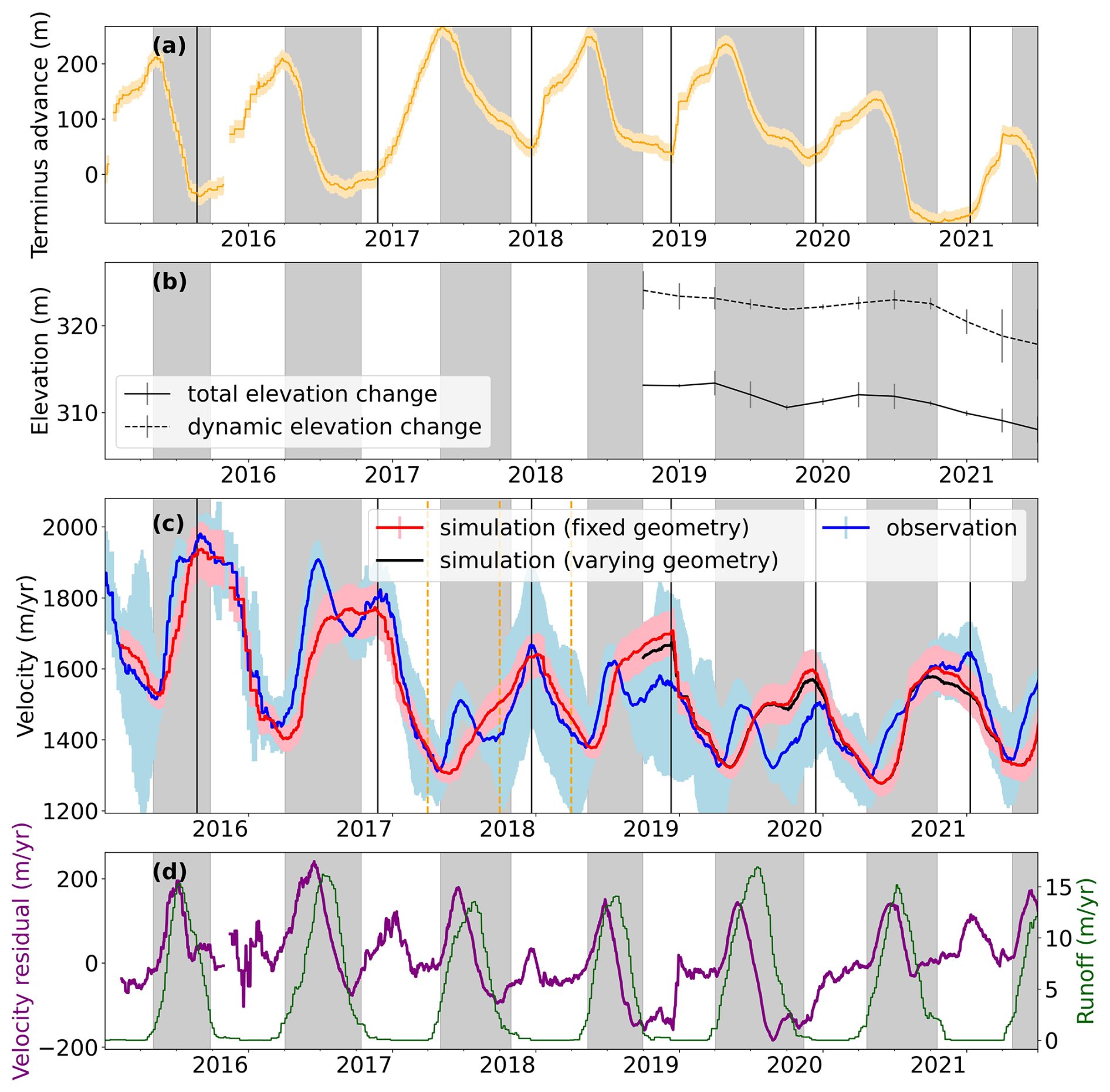
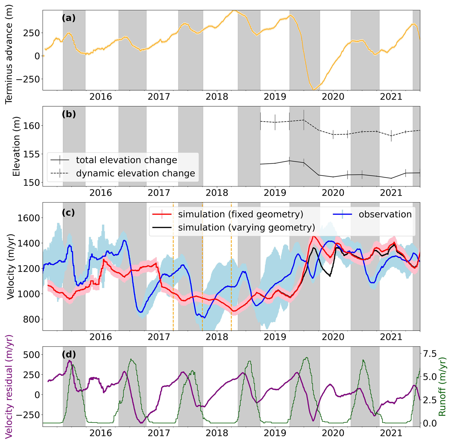
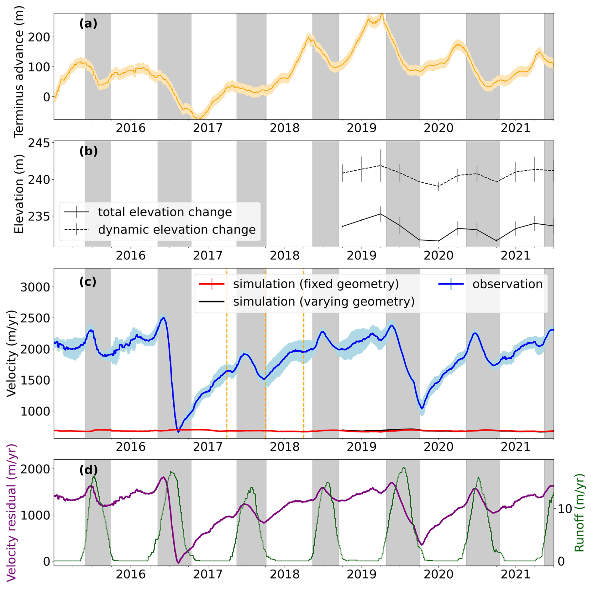
Figure 2 Time series for EQP. (a) Terminus position change time series from AutoTerm, with light yellow shading showing uncertainty. (b) Surface elevation from ICESat-2 data fusion. The dynamic elevation change is calculated by subtracting elevation change due to surface mass balance from total elevation change. (c) Observed and simulated velocity. Light blue and pink shading show the uncertainties of observations and simulations, respectively. (d) Velocity residual between observed and simulated velocity, along with the daily runoff from GSFC-FDMv1.2.1 (values are per-unit-area runoff, in m yr⁻¹). In all panes, gray vertical bars mark melt seasons using the 1st percentile of each year’s runoff as the threshold. The vertical black lines mark the onset of annual glacier retreat. The orange dashed lines in (c) marks the two periods in Fig. 9a and b, respectively.

Terminus position data come from AutoTerm (Zhang et al., 2023), a machine learning pipeline that automatically produces terminus traces with an average sampling frequency of 10 per month since 2014. We derive a time series of terminus change by calculating the sequential area changes between termini, accumulating these over time, and then normalizing this by a static glacier width of 6 km for AVA, 5 km for KUJ, 4 km for KAN, and 3 km for EQP. The area-based metrics account for both terminus shape and fjord geometry (Zhang et al., 2019), and unlike the curvilinear box method, they do not require a predefined box to represent the fjord geometry. We apply the same 40 d rolling average to smooth terminus data as described above. The uncertainties for ITS_LIVE, AutoTerm data, and simulated velocity from the terminus-driven model are represented as shaded areas in our time series figures (Figs. 2 to 5) and we present the average uncertainties in Table 1.

Figure 3 Time series for KUJ. The figure follows the same design as Fig. 2. The orange dashed lines in (c) marks the two periods in Fig. 9c and d, respectively.

Figure 4 The full record of KAN. The figure follows the same design as Fig. 2. The orange dashed lines in (c) marks the two periods in Fig. 9e and f, respectively.

Figure 5 Time series for AVA. The figure follows the same design as Fig. 2. The orange dashed lines in (c) marks the two periods in Fig. 9g and h, respectively.

We generate surface elevation data through a novel fusion of ICESat-2 data with DigitalGlobe high-resolution digital elevation models (DEMs), termed “DG-IS2-DEM” producing four DEMs per year from Fall 2018. The algorithms that generate the DG-IS2-DEMs are described in the Supplementary Information (Sect. S1). We also use ArcticDEM (Porter et al., 2022) as supplementary elevation data in locations where the DG-IS2-DEMs do not extend to the most advanced terminus position found in AutoTerm. To determine ice thickness, we subtract surface elevation data from bed elevation data from BedMachineV5 (Morlighem et al., 2022), which assimilates seafloor bathymetry and ice thickness data through a mass conservation approach (Morlighem et al., 2017). BedMachine is an estimate of the bed topography, not a measurement and carries a spatial resolution of 150 m and uncertainties of ∼ 60 m for AVA, ∼ 70 m for KUJ, ∼ 20 m for KAN, and ∼ 90 m for EQP. These low uncertainties result because each of these glaciers has radar-determined bed elevation data to within ∼ 1 km of the current terminus position (Catania et al., 2018). For both of these data sets we extract the elevation profiles along each flowline individually.

We use the runoff component in GSFC-FDMv1.2.1 (Medley et al., 2022), which provide the evolution of surface mass balance and its individual components from 1 January 1980 to 30 June 2022 at 5 d temporal resolution and 12.5 km spatial resolution on North Polar Stereographic Projection. We extract 5 d runoff time series at points in Fig. 1. The onset and cessation of runoff served as proxies for the melt season timing. Following Stevens et al. (2016), we define runoff values below the 1st percentile of each year as wintertime, and values above that threshold as summertime (Figs. 2–5).

4 Terminus-Driven model

Force balance methods can be used to understand the dynamic evolution of glaciers by examining the balance of stresses on them (van der Veen et al., 2011; Carnahan et al., 2022). However, the force balance method requires a second-order derivative of surface velocity data, which can result in large uncertainties when using satellite products. Therefore, we adopt a different approach that employs a modified force balance termed the “terminus-driven model” described by Joughin et al. (2012). This model explicitly considers the influence of dynamic changes at the glacier terminus on upstream velocity. By using the terminus-driven model and near daily velocity data, we are able to isolate the contribution of terminus variations to the observed variations in the velocity time series. The terminus-driven model is a 1-D model along the flow direction, assuming ice mélange-free conditions, a constant glacier geometry over time, and a grounded glacier. The terminus-driven model first quantify the driving stress (τ_d) at the points where we simulate velocity, expressed as

$$\begin{array}{}\text{(1)}& {\mathit{\tau }}_{\mathrm{d}}=-{\mathit{\rho }}_{\mathrm{i}}gH{\displaystyle \frac{\partial h}{\partial x}}\end{array}$$

where ρ_i is the density of ice (910 kg m⁻³), g is the gravitational acceleration (9.81 m s⁻²), H is ice thickness, h is ice surface elevation, x is the distance along the flowline with the direction from downstream to upstream. The driving stress is only calculated at the points where we simulate velocity. Secondly, the terminus-driven model examines an additional force at the water-terminating calving face, determined by the height above the fjord surface at the calving front and the density of seawater. The difference between these two forces at the terminus is expressed as

$$\begin{array}{}\text{(2)}& F={\displaystyle \frac{\mathrm{1}}{\mathrm{2}}}{\mathit{\rho }}_{\mathrm{i}}g{H}^{\mathrm{2}}-{\displaystyle \frac{\mathrm{1}}{\mathrm{2}}}{\mathit{\rho }}_{\mathrm{w}}g(H-h{)}^{\mathrm{2}}\end{array}$$

where ρ_w is the density of seawater (1028 kg m⁻³). Here, we call F the “frontal force” following the naming convention found in Joughin et al. (2012), although it has units of N m⁻¹. The force balance at the terminus requires the frontal force to be balanced upstream by the longitudinal stress, which redistributes much of the frontal force to the glacier upstream. We term the longitudinal stress in the upstream region that originates from the frontal force as τ_F(X), which pulls/opposes the glacier and enhances/reduces the original driving stress (e.g., τ_d+τ_F(X)). X is the distance between terminus and the point where we simulate velocity.

The integration of τ_F(X) along the flowline equals F and is assumed to linearly decrease upstream of the terminus to zero at the upper limit of stress coupling following Joughin et al. (2012):

$$\begin{array}{}\text{(3)}& {\mathit{\tau }}_F\left(X\right)=\mathrm{2}{\displaystyle \frac{F}{\mathit{\lambda }}}\left(\mathrm{1}-{\displaystyle \frac{X}{\mathit{\lambda }}}\right)\end{array}$$

where λ is the upper limit of stress coupling. Terminus variations cause changes in the geometry at the free calving face, consequently influencing the frontal force (F). These changes in the frontal force, subsequently, lead to modifications in the enhanced driving stress (τ_d+τ_F(X)) in the upstream region. Thus, the calculation of F and τ_F(X) over time requires elevation data along the profile.

In the laminar flow model or the shallow ice approximation, when basal sliding is zero, the surface velocity has a linear relationship with the cube of driving stress (n=3):

$$\begin{array}{}\text{(4)}& V={\displaystyle \frac{\mathrm{1}}{\mathrm{2}}}AH{\mathit{\tau }}_{\mathrm{d}}^{\mathrm{3}}\end{array}$$

where A is a constant from Glen's flow law (van der Veen, 2013) and V is surface velocity. Such a linear relationship also applies when the driving stress is mainly balanced by lateral drag (van der Veen, 2013):

$$\begin{array}{}\text{(5)}& V={\displaystyle \frac{\mathrm{1}}{\mathrm{2}}}A{\left({\displaystyle \frac{{\mathit{\tau }}_{\mathrm{d}}}{H}}\right)}^{\mathrm{3}}{W}^{\mathrm{4}}\end{array}$$

where W is half of the glacier width. Based on the above two models and following the method designed by Joughin et al. (2012), we assume a linear relationship between velocity and the cube of the enhanced driving stress: τ_d+τ_F(X). Finally, the predicted velocity from terminus changes is thus given by:

$$\begin{array}{}\text{(6)}& {\displaystyle \frac{V\left(X,t\right)}{V_{\mathrm{0}}}}={\left({\displaystyle \frac{{\mathit{\tau }}_{\mathrm{d}}+{\mathit{\tau }}_F\left(X\right)}{{\mathit{\tau }}_{\mathrm{d}}+{\mathit{\tau }}_{F_{\mathrm{0}}}}}\right)}^{\mathrm{3}}\end{array}$$

where V₀ is a reference velocity at the same location as velocity observations and ${\mathit{\tau }}_{F_{\mathrm{0}}}$ is the τ_F(X) corresponding to the reference velocity. Following Joughin et al. (2012), for each year, we use the minimum velocity observation as the reference velocity and calculate ${\mathit{\tau }}_{F_{\mathrm{0}}}$ based on the terminus position nearest the date of the reference velocity. Using Eq. (6), we simulate velocity observations at both the blue and red points in Fig. 1 using corresponding geometry profiles along each flowline. Then, we average the simulated velocity across all the flowlines at each cross-section to produce mean velocity time series in a manner consistent with the observed velocity.

We vary λ for each glacier and choose the one that produces the lowest mean difference between observations and simulated velocity (Table S1). The mean difference is determined by:

$$\begin{array}{}\text{(7)}& \left({\sum ^N}_n{\sum ^{\mathrm{6}}}_m{\displaystyle \frac{\mathrm{abs}(V_{m,n}^{\mathrm{model}}-V_{m,n}^{\mathrm{obs}})}{V_{m,n}^{\mathrm{obs}}}}\right)÷(N\times \mathrm{6})\times \mathrm{100}\mathit{\%}\end{array}$$

where 6 is the total number of velocity points on the same cross section and N is the total number of time steps in the entire time series. We use the red points in Fig. 1 to find an optimal upper limit of stress coupling (λ). The optimized λ values are then used to simulate velocity time series at the blue points in Fig. 1, which allow us to test the sensitivity of the velocity position to the results.

We also calculate the velocity residual by subtracting the simulated velocity with fixed geometry from the observed velocity. The velocity residual refers to the portion of the velocity that is not associated to terminus changes but is affected by other factors, such as runoff. We then plot residuals overlapping with runoff for ease of comparison (Figs. 2–5). We assign the uncertainty of the terminus change (Zhang et al., 2023) as the error of X in Eq. (3), and propagate this error to obtain the uncertainty in the simulated velocity.The elevation uncertainties are not directly included, as our model assumes invariant geometry (following Joughin et al., 2012).

Although the terminus-driven model assumes invariant geometry, we analytically examine the impact of seasonal variations in surface elevation on velocity simulations, offering a complementary sensitivity test for elevation-related effects. Specifically, we leverage the new time-varying DG-IS2-DEM and periodically update the elevation profiles each quarter from Fall 2018, maintaining profile fixed within each quarter. We produce a simulated velocity for all glaciers with and without time-varying surface elevation to evaluate the impact of seasonally-varying surface elevation change on velocity. For the fixed geometry simulations, we choose a time step from DG-IS2-DEM with an extent that aligns best with the position of the terminus when it is most advanced. This provides the most complete elevation profile across the terminus region. For EQP, KAN, and AVA we choose the October 2019 DG-IS2-DEM and for KUJ, we use the April 2019 DG-IS2-DEM time step. To further investigate the impact of changing elevation on the simulation results, we consider only KUJ as an example and conduct two experiments using artificially modified surface elevation; (1) we shift the entire elevation profile vertically by ± 10–20 m and; (2) we alter the surface slope by ± 2 % within the 2 km-frontal region.

5 Results

Our comparative analysis of model outputs, runoff data, and velocity observations reveals that the seasonal velocity variations of all four glaciers exhibit three distinct patterns, which align with those identified by Moon et al. (2014). We find that each glacier exhibits two of these patterns, occurring either alternately or simultaneously each year. Following the velocity-pattern classification of Moon et al. (2014), we describe each glacier’s seasonal behavior as a combination of patterns: EQP and KUJ exhibit patterns consistent with type-1 plus type-2, whereas KAN and AVA exhibit patterns consistent with type-2 plus type-3.

5.1 Comparison between velocity simulation and observations

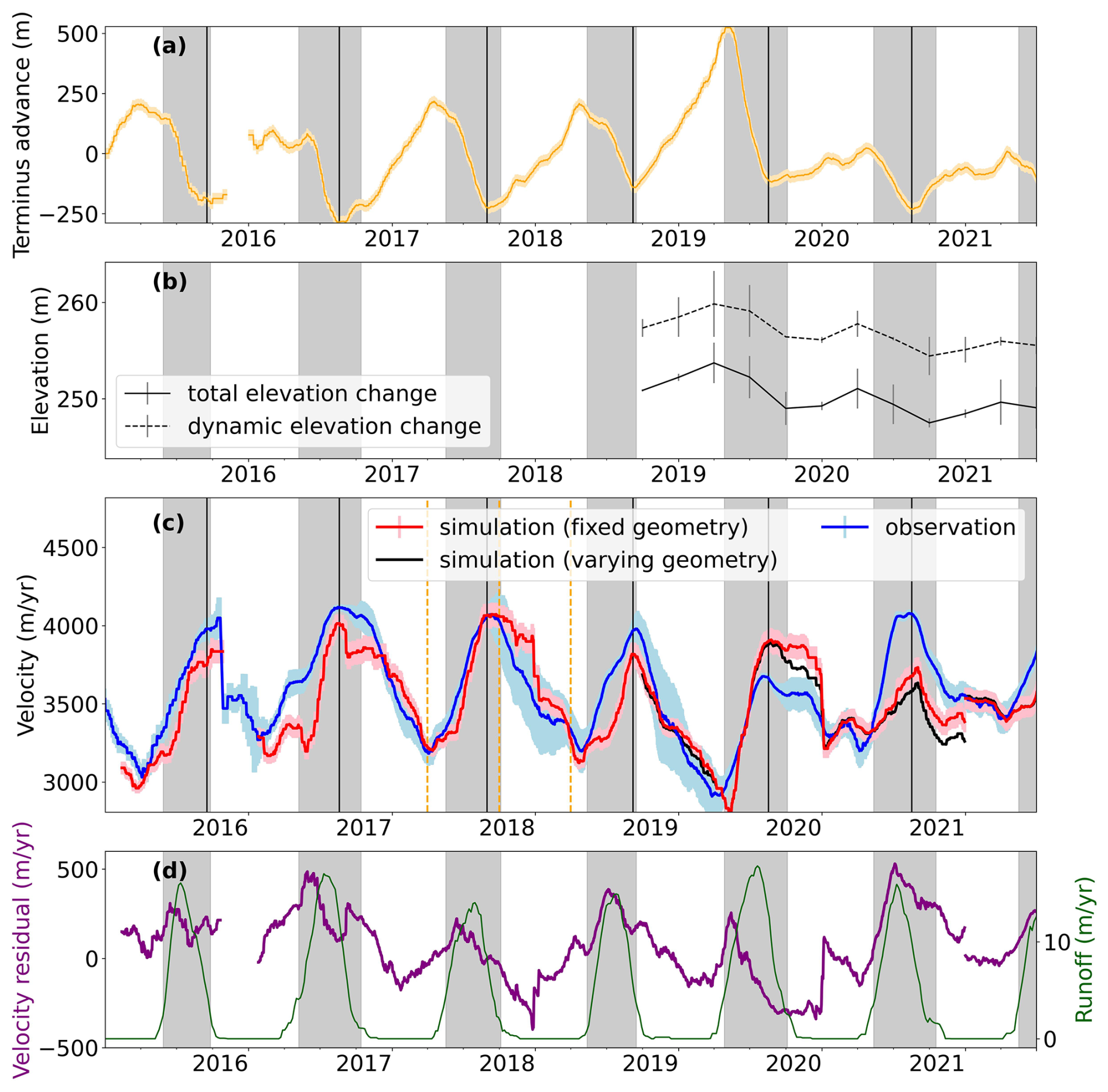
We compare the simulated velocity time series with velocities from satellite observations to determine whether seasonal velocity variations are influenced primarily by terminus change, co-influenced by subglacial hydrological system, or entirely independent of terminus change. We find that the terminus-driven model, after tuning λ, produces a good match to velocity observations for KUJ and EQP (Figs. 2 and 3) but not for KAN and AVA (Figs. 4 and 5). Note that λ only scales the amplitude of the simulated velocity without affecting its phase or temporal pattern. This indicates that both EQP and KUJ have type-1 velocity behavior. This is supported by the coincident timing of the end of terminus retreat and the peak summertime velocity (vertical black lines in Figs. 2 and 3), even in instances when retreat continues beyond the end of the melt season (Fig. 2). This is also supported by the percentage difference between the simulated and observed velocities over all years, which are 5.0 % for KUJ and 6.2 % for EQP (Table S1), with correlations of 0.73 and 0.67, respectively (Fig. 6) and small residuals (Figs. 2 and 3). The λ chosen based on minimizing the difference between observed and modeled velocity are EQP = 10 km, KUJ = 20 km, KAN = 25 km, and AVA = 25 km (Table S1). However, KAN and AVA’s seasonal velocities are not primarily driven by terminus variation, so we do not consider the estimation of λ valid for these glaciers.

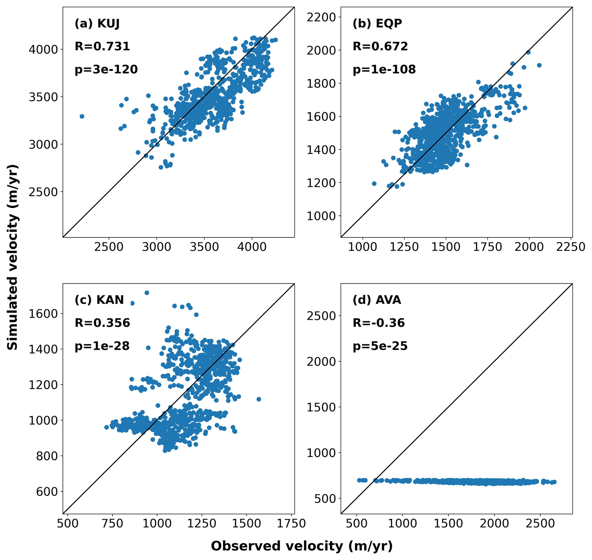
Figure 6 Scatter plot showing the comparison between simulated and observed velocity for KUJ, EQP, KAN, and AVA. The 1:1 line is as shown for each.

For AVA and KAN, we find that simulated velocities differ substantially from the observed velocities suggesting that the terminus-driven model is insufficient to explain the observed velocities and that velocity change is not primarily driven by terminus fluctuations. For AVA, we find a poor correlation between observed and simulated velocity (−0.36; Fig. 6) and residuals are just slightly smaller than the velocity observations themselves. For KAN, the simulated and observed velocities are out of phase but of similar magnitude, producing small residuals (Fig. 4) but a poor correlation, R=0.36 (Fig. 6). Although our simulation results indicate no significant correlation between seasonal-scale glacier velocity changes and terminus variations at KAN, Kane et al. (2020) found a large, full-thickness calving event induced speed up in the frontal region of KAN on an hourly time-scale.

5.2 Non-terminus velocity processes

Although the terminus-driven model adequately resolves the majority of seasonal velocity variability for KUJ and EQP, the velocity residuals reveal additional sub-seasonal velocity changes that are not related to terminus change. One such signal is an additional pulse in velocity (acceleration and deceleration) that occurs near the middle of the melt season for all glaciers (Figs. 2–5), meaning that all glaciers have type-2 behavior. For KUJ, these melt-season pulses are not evident in the original velocity time series, but only become apparent in the velocity residuals, which further validates the effectiveness of our method in decomposing the coupled seasonal velocity variations of glaciers. We find that these mid-summer residual speed ups account for more than 80 % of the observed summertime velocity signal across all glaciers, with KAN and AVA exhibiting a higher percentage (91 % and 86 % respectively) than EQP and KUJ (84 % and 82 % respectively). We typically observe a lag time between the peak of the velocity residual followed by the peak of summer runoff (Figs. 2–5). We conduct cross correlation analysis between the velocity residual and runoff to assess the time lag between the two and quantify the maximum correlation coefficient, thereby investigating the extent to which velocity is influenced by runoff. These lag times differ among glaciers, measuring 24 d for KUJ, 22 d for EQP, 47 d for KAN, and 51 d for AVA. The maximum correlation coefficients are 0.49 for KUJ, 0.73 for EQP, 0.67 for KAN, and 0.67 for AVA (Fig.  7).

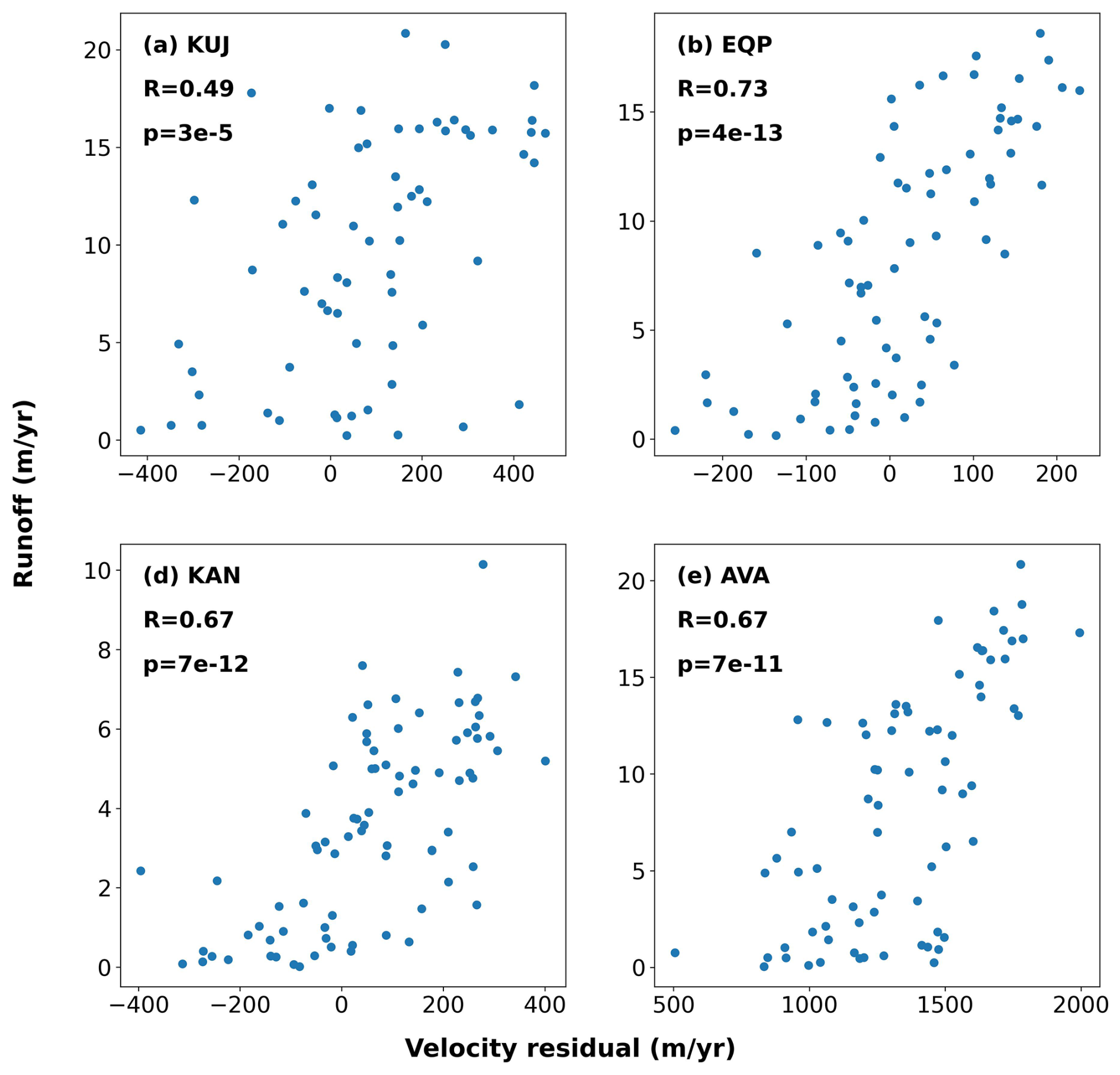
Figure 7 Scatter plot showing the comparison between velocity residual and runoff for KUJ, EQP, KAN, and AVA. The phases of velocity residual have been adjusted to achieve the maximum correlation coefficient.

For KAN and AVA, we observe accelerations during winter (during terminus advance); velocities then plateau before the onset of the melt season in the following year, and early melt season accelerations with the annual maximum velocity reached in the middle of the melt season (Figs. 4 and 5). The terminus-driven model does not capture wintertime acceleration because across all glaciers the terminus is advancing in winter. For KAN, the model predicts slight deceleration in winter (Fig. 4). For AVA, the simulated velocity lacks significant seasonality because (1) the seasonal terminus variations are small (Fig. 5), and (2) the frontal region has a very low surface slope (Fig. S6). Together, these two reasons lead to small change in frontal force F (Eq. 2), and thus little seasonality in simulated velocity. For reference, the averaged seasonal range in terminus position is 138 m for AVA, while EQP is 217 m, KAN is 370 m, and KUJ is 400 m.

5.3 Experiments with seasonally varying surface elevation

We investigate the influence of changing surface topography by comparing the velocity simulated using a fixed geometry against the velocity simulated using a seasonally varying surface elevation from 2018–2022. We find minimal differences between these results for all glaciers (black versus red lines in Figs. 2–5). Using KUJ as an example, the results from two analytical experiments involving artificially modified elevation profiles suggest that terminus-driven velocities are relatively insensitive to spatially uniform along-flow changes in surface elevation. In contrast, they show a high sensitivity to changes in surface slope (Fig. 8): a 2 % absolute change in slope leads to a 2 % change in average velocity and a 6 % change in peak velocity. This result is important for providing context for interpreting the results of this model and our assumptions.

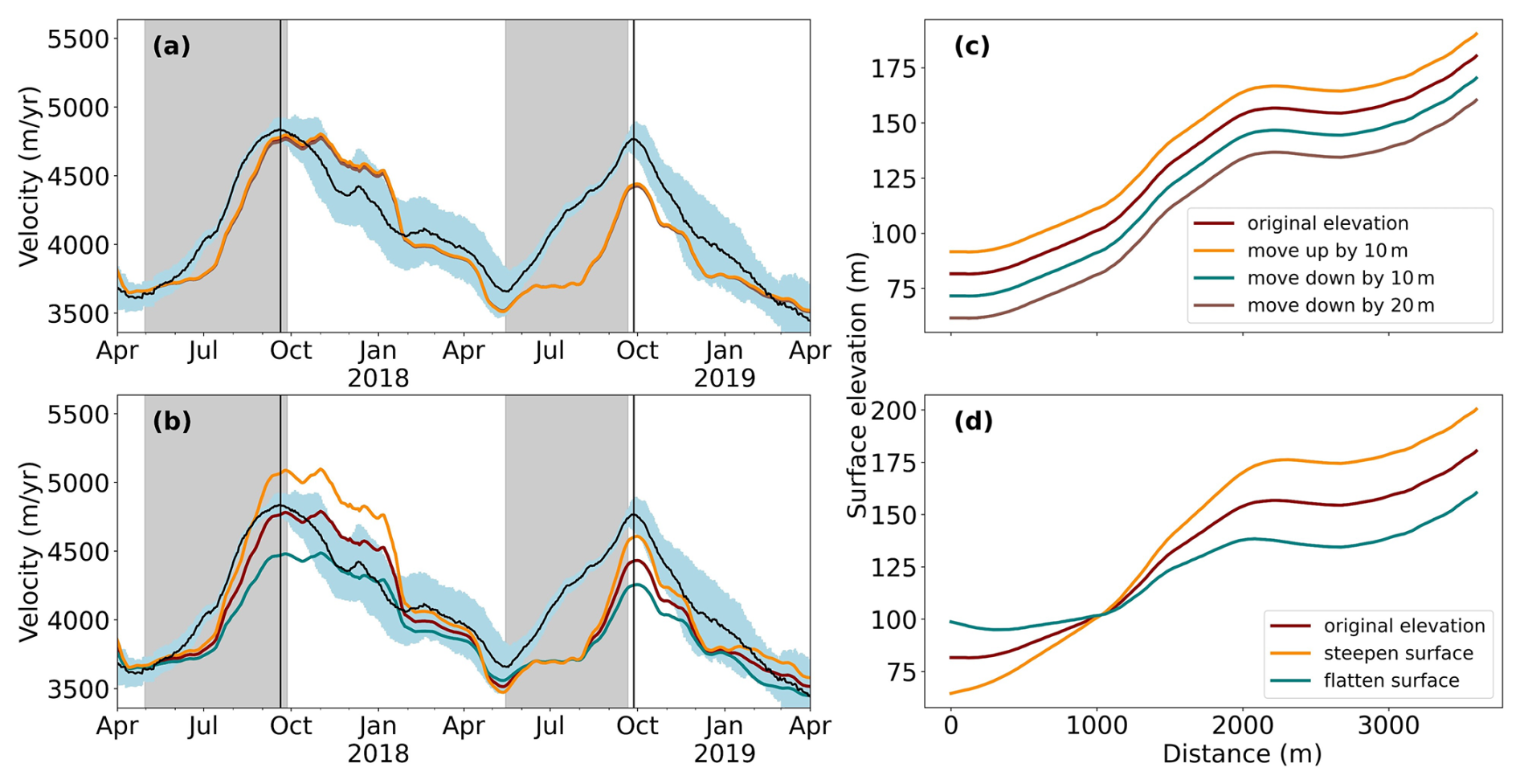
Figure 8 Experiment results for KUJ using artificially modified surface elevations. Panels (a) and (c) correspond to each other, as do (b) and (d). The blue shaded area represents observation uncertainties. Vertical black lines indicate the onset of the annual glacier retreat, and gray shaded vertical bars denote the melt season. In panel (d), the surface slope is altered by ±2 % within the 2 km frontal region.

6 Discussion

Using observations with high temporal resolution and a terminus-driven model to simulate velocity variations resulting solely from terminus change, we investigate the controls on sub-seasonal velocity changes for four GrIS outlet glaciers and find that in all cases, glacier velocity responds to multiple compounding processes. The seasonal velocity changes of two glaciers (KUJ and EQP) show a strong correspondence to seasonal terminus variation (type-1). All study glaciers experience sub-seasonal peaks in velocity that occur in the middle of the melt season (type-2) and, AVA and KAN exhibit wintertime speedup that occurs when their termini are advancing (type-3) (Figs. 4 and 5). Our combined pattern descriptions offer a different perspective from Vijay et al. (2021), which classified EQP and KAN as type-3, identified AVA as type-2 in 2018 and type-3 in 2017 and 2019, and did not classify KUJ. This difference reflects our use of high-temporal-resolution observations together with a simplified physical model, which allows us to identify the presence of multiple coexisting patterns and link them to interacting processes. We emphasize that these different classifications are not contradictory; rather, they arise from different methodological focuses (pattern-based annual classification vs. process-informed sub-seasonal analysis) and together enrich our understanding of glacier seasonal dynamics.

We hypothesize that the peaks in velocity residuals observed for all glaciers during the middle of the melt season (Figs. 2–5) are the result of meltwater-driven acceleration and subsequent evolution of the subglacial drainage system (Moon et al., 2014; Vijay et al., 2019). Early in the melt season, the subglacial drainage system is not fully channelized (Andrews et al., 2014), thus as meltwater availability begins to increase (marked by increasing runoff in early summer), subglacial water pressure increases, enhancing basal sliding by reducing friction between the ice and the bed (Bartholomew et al., 2010; Bartholomaus et al., 2008; Andrews et al., 2014). As the melt season progresses, the drainage system becomes more channelized, allowing for more efficient water drainage (Andrews et al., 2014; Schoof, 2010). Consequently, the available meltwater decreases, producing a reduction in glacier speed. This change in efficiency of the subglacial drainage system may explain the lag between peak velocity residual and peak runoff as has been shown by previous authors (King et al., 2020). The more readily the subglacial drainage system channelizes, the earlier the peak velocity residual occurs relative to peak runoff. Beyond the melt season, the impact of terminus retreat on seasonal velocities can become more pronounced. For example, EQP typically has a melt season that ends in October, but the terminus continues to retreat until December/January (the vertical black lines are usually behind the end of the gray bar in the same year in Fig. 2). This produces a wintertime velocity peak that is coincident with the most retreated terminus of EQP and is distinct from the melt-season peak.

To further explore the velocity increases that occur in summer, we examine the along-flow variability in velocity to determine how far upstream velocity changes occur (Fig. 9). Our hypothesis is that changes in basal lubrication will be widespread over the region where water enters the bed, but downstream of the equilibrium line (Catania et al., 2017). To confirm that runoff drives the summertime speed up, we compare the along-flow spatial pattern of velocity change that occurs in the summer melt season of 2017 for EQP where summer velocity peaks are strongest (Apr 2017–Sep 2017; Fig. 9a) and the subsequent time period when runoff is low and the velocity is primarily influenced by terminus changes (Oct 2017–Mar 2018; Fig. 9b). The idea is that runoff-driven expansion of the subglacial drainage system would produce velocity changes that extend far inland from the terminus, while terminus-driven increases in velocity would decay rapidly from the terminus (Smith et al., 2017). The rapid decline in speed with distance from the terminus is expected when a glacier is terminus-driven because of the reduction in the terminus force with distance from the terminus (Joughin et al., 2012). Conversely, elevated inland velocities are typical for melt-driven acceleration (Sundal et al., 2011) because meltwater percolates throughout a large portion of the ablation zone (Andrews et al., 2014), which extends about 70 km inland of the terminus for EQP (Noël et al., 2019).

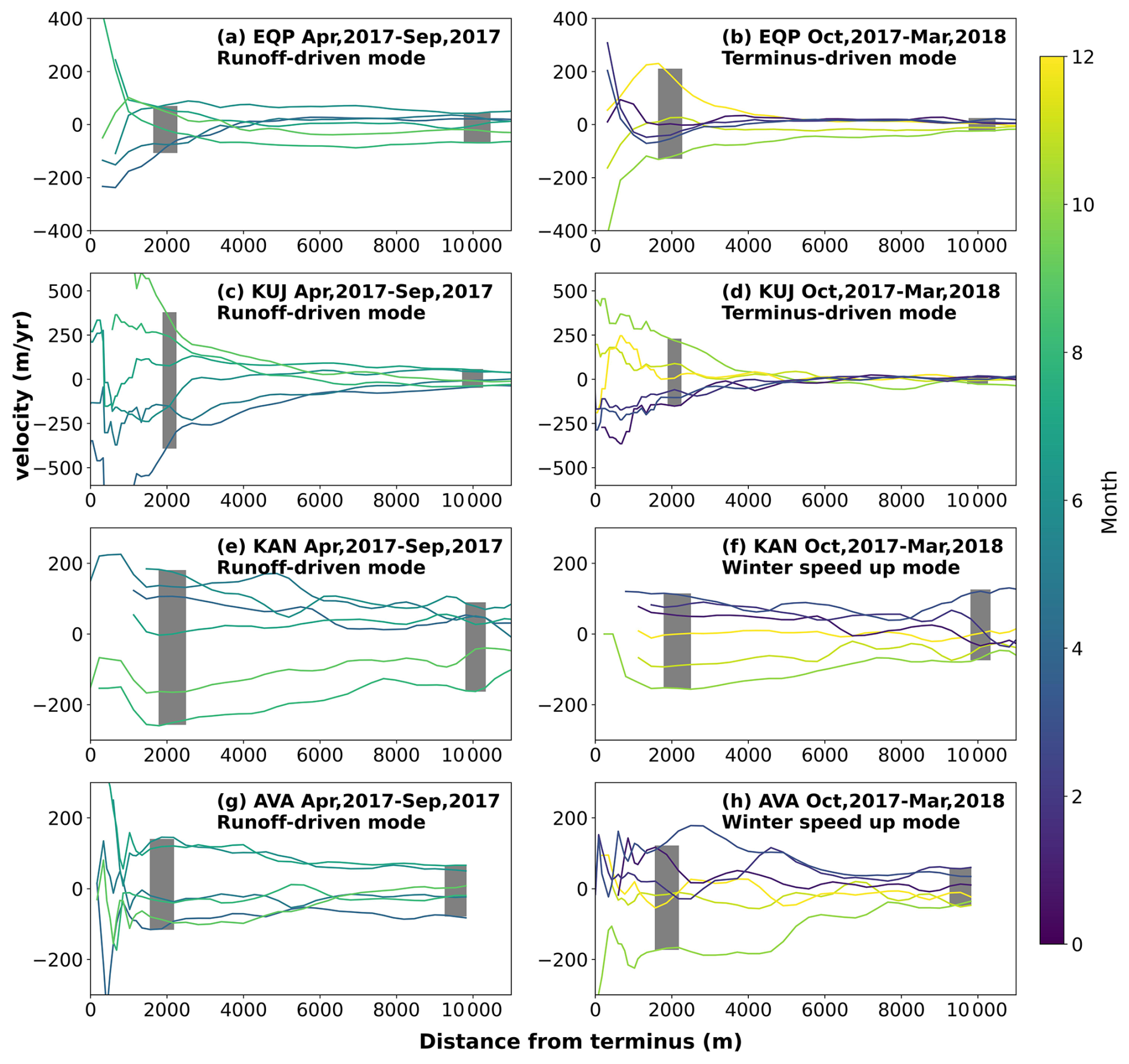
Figure 9 Velocity profiles over time for EQP, KUJ, KAN, and AVA. The average velocity profile has been subtracted for a better display of changes over time. The original velocity profiles are shown in Fig. S7. The shaded areas indicate regions where we obtain velocity variations in the frontal (left) and upstream (right) sections. Left column (a, c, e, g) Melt-season profiles for EQP (a), KUJ (c), KAN (e), and AVA (g). Right column (b, d, f, h) Post-melt-season profiles for EQP (b), KUJ (d), KAN (f), and AVA (h), when velocity is primarily influenced by terminus changes.

We choose a distance of 10 km upstream from the terminus to represent the inland distance and compare the range in velocity in this location to the range in velocity found at a location that is 2 km from the terminus. A larger ratio of velocity range between the upstream and the frontal region, in conjunction with the correlation between velocity residuals and runoff data, indicate that the velocity is likely driven by runoff. For EQP, we find that in the summer (Apr–Sep) the upstream velocity range is 64 % of that observed at the terminus (Fig. 9a) while in winter (Oct–Mar) the upstream velocity is just 12 % of what is observed at the terminus (Fig. 9b). In addition to EQP, we also find that in summer (Apr–Sep) the upstream velocity ranges for both KAN and AVA are both 56 % of that observed at the terminus (Fig. 9e and g). Thus, we conclude that summer accelerations of EQP, KAN, and AVA are strongly caused by runoff, as they are more noticeable upstream compared to the velocity changes in EQP during the winter, which are driven by terminus changes. For KUJ, the ratio of velocity range between the upstream and frontal region is 13 % in summer (Apr–Sep) (Fig. 9c), slightly larger than the 10 % ratio observed in winter (Oct–Mar) (Fig. 9d). Based on this observation, along with the correlation between KUJ's velocity residual and runoff (Fig. 7a), we conclude that runoff also influences the velocity changes of the KUJ glacier during the summer, although its impact is not as pronounced as that on the other three glaciers.

While AVA and KAN experience mid-summer velocity pulses similar to EQP, they do not exhibit notable terminus-driven seasonal acceleration (Figs. 4 and 5) and instead accelerate in winter. This is suggested by the poor correlation between velocity changes and terminus changes for these glaciers. Although our simulation results indicate no significant correlation between seasonal-scale glacier velocity changes and terminus variations at KAN, Kane et al. (2020) found a large, full-thickness calving event induced speed up in the frontal region of KAN on an hourly time-scale. To examine wintertime acceleration, we investigate the along-flow pattern of velocity change similar to above (Fig. 9f and h). For both glaciers we find significant inland acceleration in winter. For KAN, the range in upstream (farther from the terminus) velocity during winter is 72 % of the range in frontal velocity and for AVA, the range in upstream velocity is 36 % of the range of frontal velocity, which is larger than terminus-driven upstream velocity range that was observed for EQP (Figs. 9f and h versus b). We hypothesize that the elevated range of KAN and AVA's upstream velocities in winter suggests that winter acceleration is due to enhanced extensive basal slip.

For many parts of Greenland, basal water is generated year-round because of friction at the ice-bed interface and geothermal heat (Karlsson et al., 2021). During the onset of winter, refreezing of available basal water (Boon and Sharp, 2003) and viscous deformation over subglacial conduits (Vieli et al., 2004; Bartholomaus et al., 2011) can obstruct the drainage system. Consequently, water becomes trapped within an inefficient drainage network, leading to increased water pressure and winter acceleration (Vijay et al., 2019). The winter acceleration phase ends when the melt season begins to supply significant volumes of additional water to the subglacial system, which increases basal water pressures causing summertime acceleration (Davison et al., 2020).

Our examination of how our model performs further upstream of the terminus (Supplementary Information) informs the transmission distances for terminus perturbations. Felikson et al. (2017) and Felikson et al. (2021) quantified the Péclet number (Pe) for the glaciers in our study. Most of the dynamic mass loss occurs downstream of Pe = 3 (Felikson et al., 2021), a threshold that aligns closely with the upper limit of stress coupling we derived from our analysis. The Pe = 3 locations for these glaciers are: KAN = 32 km, AVA = 27 km, KUJ = 28 km, and EQP = 15 km (Felikson et al., 2021). The values of λ chosen by minimizing the difference between observed and modeled velocities are 10 km for EQP and 20 km for KUJ. For KAN and AVA, seasonal velocities are not primarily driven by terminus variation, so we do not consider the estimation of λ valid for these glaciers. Notably, the λ values for EQP and KUJ are shorter than their respective Pe = 3 locations. We assume a constant upper limit of stress coupling along the profile and use a simplified one-dimensional terminus-driven model, both of which may influence our estimations.

Impact of observed seasonal elevation changes

The availability of seasonally-resolved elevation change allows us to investigate the degree to which outlet glacier terminus velocity is sensitive to changing surface elevation. We find that the seasonal elevation changes for EQP, KAN, KUJ, and AVA show limited spatial variation along the flow (Fig. 10). Quantitatively, for each profile, the standard deviation along the profile (i.e., spatial variation with distance) averages only 22 % of the profile’s mean value. This low ratio indicates that the profiles are relatively uniform along flow. Thus, the seasonal elevation change is largely uniform across the DEM and these elevation changes do not significantly alter terminus-driven velocity (black lines in Figs. 2–5). This aligns with our experimental results that suggest that vertical shifts in elevation have a limited contribution to velocity seasonality (Fig. 8a) but that steepening the surface elevation will cause stronger velocity responses to terminus variations (Fig. 8b).

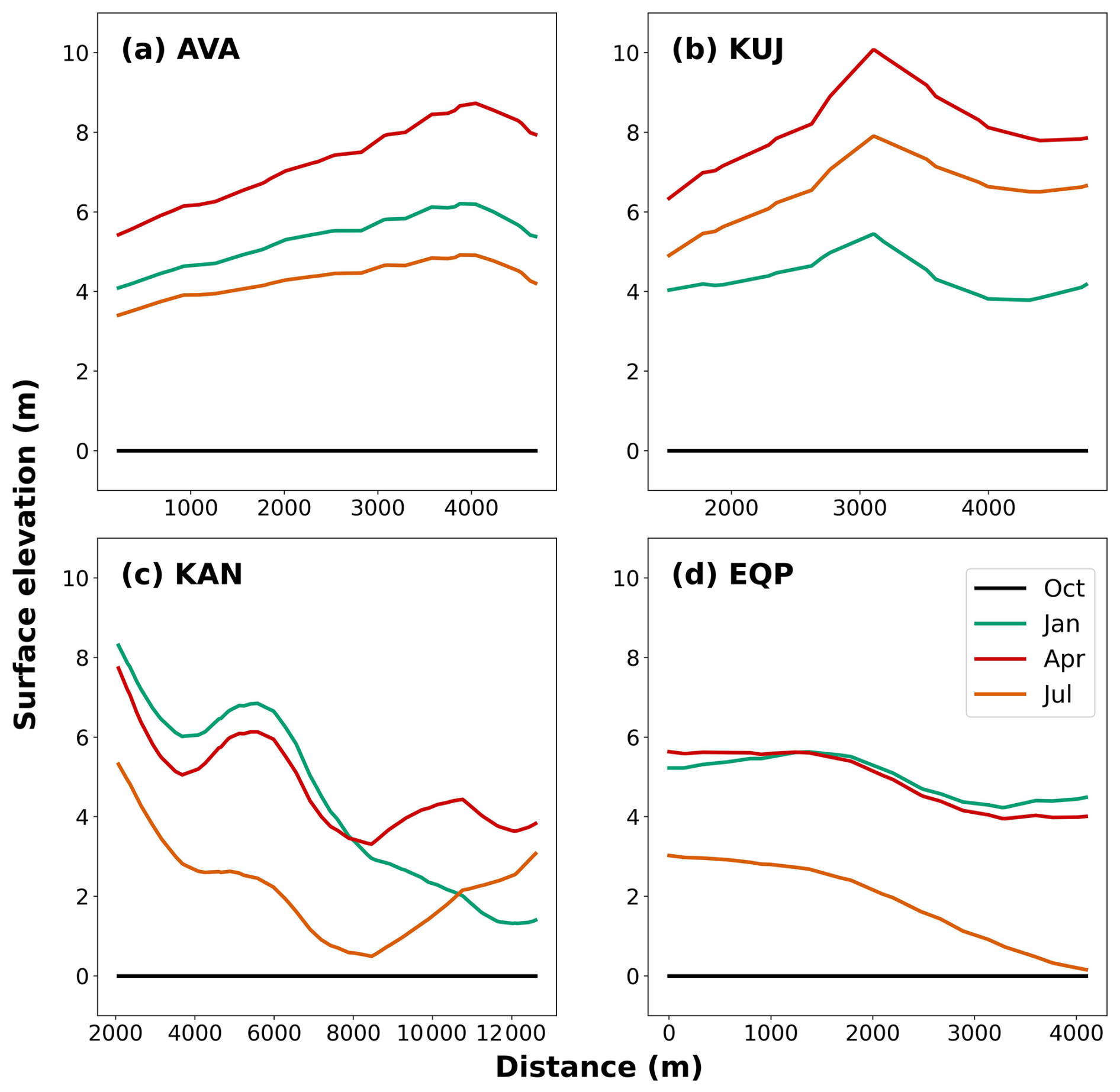
Figure 10 Surface elevation difference profiles for AVA, KUJ, KAN, and EQP in 2019 relative to the October profile. Profile lengths are limited by the overlapping area of the DG-IS2-DEM.

7 Limitations and Outlook

We recognize that the choice of the terminus-driven model to explore how outlet glacier velocity might respond to terminus change is simplified over that from numerical results. There are several important limitations that merit further discussion. Seasonal elevation change is not yet available widely and may be worth including for some glaciers, particularly ones that are experiencing changes in slope near the terminus, which might influence ice velocity. While our experiments indicate insensitivity to uniform vertical elevation changes under the assumptions of this model, we cannot rule out that other physical models (e.g., including basal sliding or full stress coupling) might produce different results. Future work with higher-order models could test the robustness of this finding. The model only looks at the impact of terminus change on ice velocity and thus many important processes that control ice velocity are lumped into the examination of the velocity residuals. Here we have considered processes such as melt-driven changes in velocity and wintertime acceleration related to meltwater at the bed. Other factors such as air temperatures (Walter et al., 2012; Carr et al., 2013) may play a secondary role, but terminus change and meltwater are likely the dominant drivers of seasonal and inter-annual variations.

In addition to these limitations, the model only captures longitudinal stresses, not lateral stresses. Since floating ice can experience velocity variations that are driven by nearby velocities on the grounded ice through transmission of lateral stress, the model is not appropriate for use on floating ice. The terminus-driven model importantly only applies close to the terminus since by definition, the frontal force F linearly decreases upstream of the terminus to zero at the upper limit of stress coupling.

Despite these shortcomings, the terminus-driven model provides a means to isolate the impact of seasonal terminus variations on outlet glacier velocity without numerical methods. Thus, it offers a quick assessment of how terminus variations impact glacier velocity across different glaciers, and how this impact changes over time. Future work could examine how seasonal velocity patterns vary from glacier to glacier and how those patterns change during periods of sustained year-over-year terminus retreat. Furthermore, the terminus-driven model helps illustrate that glaciers exhibit multiple, coexisting seasonal velocity patterns, suggesting that categorization of glacier velocity resulting from a single pattern may be insufficient to capture the full seasonal behavior.

8 Conclusions

We apply a terminus-driven model to elucidate the degree to which seasonal terminus change can explain seasonal velocity variations for four glaciers in Central West Greenland. The comparison between simulated and observed velocity suggests that all glaciers experience multiple drivers of velocity change. Some glaciers experience seasonal velocity changes that are dominated by terminus change and some glaciers do not respond to terminus change because either the terminus change is too small to be impactful and/or other processes dominate velocity, notably wintertime acceleration. Importantly, velocity residuals allow for us to see that runoff-driven acceleration occurs for all glaciers but its impact is limited to the early melt season. We present a new fusion of elevation products that resolve seasonal elevation changes for our study glaciers. When integrated into our model we do not find a significant difference between simulated velocities driven by terminus change assuming a fixed surface elevation versus those with an evolving surface elevation. We show that this is because the observed seasonal elevation change is largely the result of a vertical shift in surface elevation with no noticeable slope change, which would drive a velocity response. Our study highlights how a simple model can be used to examine the impact of terminus change on near-terminus velocity and allows a method for distinguishing the controls on seasonal velocity change of outlet glaciers. Moreover, the same framework could be applied to investigate the long-term changes in glacier dynamics with adequate historical data.