Evidence and interpretation of non-linear recession behaviour in a periglacial cliff at Port Foster, Deception Island (South Shetlands, Antarctica)

Cliff erosion in periglacial coastal environments is governed by complex interactions between thermal, hydrological, and marine processes, often resulting in non-linear and spatially heterogeneous behaviour. However, most existing studies rely on linear models that may not adequately capture threshold responses and episodic dynamics, particularly in data-scarce polar regions such as Antarctica. This study investigates long-term cliff erosion patterns in a periglacial coastal setting by applying linear and non-linear statistical modelling to a multitemporal dataset. The analysis focuses on the coastal bluffs of Port Foster, Deception Island (South Shetland Islands, Antarctica), using a unique 66 year record (1956–2022) derived from historical aerial imagery and high-resolution satellite data. Shoreline positions were extracted through photogrammetric processing and analysed using a transect-based framework, incorporating both linear and non-linear (quadratic and sigmoidal) least squares regression models with uncertainty-weighted parameters. Results reveal a transition from relatively stable conditions to accelerated retreat after ∼2000, with maximum change rates reaching up to 5 m yr⁻¹ in central sectors of the study area. Non-linear sigmoidal models outperform linear approaches in capturing this behaviour, particularly in identifying inflection points in erosion dynamics. The observed patterns are interpreted as the result of a coupled coastal–periglacial system, where spatial variability in permafrost conditions and hydrological processes governs material weakening, while marine forcing acts primarily as a triggering mechanism. These findings highlight the importance of incorporating non-linear approaches into the analysis of coastal change in polar environments and provide new insights into the dynamics of Antarctic periglacial coasts, with implications for monitoring and infrastructure management in vulnerable coastal sectors.

1 Introduction

The dynamic of polar coastlines is governed by a complex interplay of sea, ice, permafrost, and soil. These systems are highly sensitive to climatic warming, particularly in the Arctic and Antarctic regions, where the most visible impact is coastal retreat linked to accelerated erosion processes (Irrgang et al., 2022; Liew et al., 2022; Aga et al., 2024;). Although less frequent, shoreline progradation also contributes to coastal evolution. Coastal change is driven by interacting oceanographic, terrestrial, periglacial, and paraglacial processes that modulate shoreline position and sediment transport, influencing nutrient, carbon, and pollutant fluxes across nearshore zones. Coasts underlain by permafrost are especially vulnerable to temperature increases. Air warming accelerates thawing both from the surface and laterally through exposed cliff faces, increasing their susceptibility to mass wasting and sediment loss (Li et al., 2023; Wang et al., 2023). These transformations are expected to intensify under continued warming, exacerbated by declining sea ice extent and rising sea levels (Barnhart et al., 2014b; Bamber et al., 2019; Sun et al., 2023; Gilbert and Holmes, 2024). Quantitative assessments of these changes are essential for anticipating future erosion trajectories and for informing adaptation strategies in polar environments.

Globally, around 52 % of shorelines comprise cliffs, bluffs, coastal escarpments and other steep landforms (Young and Carilli, 2019). These abrupt coastal systems are shaped by a variety of interdependent processes – marine, subaerial, and anthropogenic – often exhibiting spatial and temporal variability in erosion patterns (Sunamura, 1992, 2015; Davidson, 2021). Where sediments are fine-grained or poorly consolidated, retreat is typically more pronounced and less predictable. These coastal environments are subject to highly complex erosion processes, particularly where softer materials dominate (Prémaillon et al., 2018). In such settings, sediment supply is mediated by fluvial and estuarine contributions and conditioned by geological structure. Wave and tidal parameters modulate sediment redistribution, while sea-level rise and increased storm intensity are expected to heighten erosion risks in the coming decades (Nicholls and Cazenave, 2010; Griggs and Reguero, 2021). As a result, coastal cliff retreat rates are expected to intensify, complicating future predictions (Trenhaile, 2011; Limber et al., 2018; Matsumoto et al., 2024). These changes pose significant challenges for long-term prediction and necessitate precise tools for monitoring, evaluating and modelling coastal response (Balaji et al., 2017; Schoonees et al., 2019).

In this context, understanding both past and present shoreline behaviour becomes vital for coastal management, allowing for site-specific adaptation strategies (Burningham and Fernandez-Nunez, 2020). The seminal work of Tanner (1978) presents a framework for quantifying spatio-temporal variations in coastal position and has become a cornerstone methodology, the Shoreline Change Analysis (SCA) for assessing erosion trends and informing management. While numerous tools and techniques exist to implement SCA, their effectiveness hinges on the availability of long, continuous datasets and the suitability of statistical models for representing complex shoreline dynamics. SCA employs Transect-Based Methods (TBMs), where shoreline positions intersect a series of transects anchored to a baseline, facilitating the evaluation of forecasting techniques (Dolan et al., 1978; Srivastava, 2005). TBMs are usually integrated as an external application in Geographic Information Systems (GIS) to take advantage of spatial data processing and analysis. Some examples include BeachTools (Zarillo et al., 2008), Quantitative shoreline change analysis (SCARPS in Jackson, 2004), and Digital Shoreline Analysis System (DSAS in Danforth and Thieler, 1992) which has been an ArcGIS extension since 1992 and the latest standalone version (Himmelstoss et al., 2024) eliminates the need for database import/export. Open-source alternatives such as ODSAS (Gómez-Pazo et al., 2022) and AMBUR (Jackson, 2010; Jackson et al., 2012) provide flexible statistical and geospatial tools within R's ecosystem. Alternative approaches for coastline discretisation include dynamic segmentation (Li et al., 2001), area-based methods (Ali, 2003), and non-linear Gaussian-distribution-based estimation for coastline change measurement (Heo et al., 2009; Kupilik et al., 2017). TBMs have become a standard for shoreline behaviour analysis (Sam and Gurugnanam, 2022; Albuquerque et al., 2013) in temperate coastal environments (Mishra et al., 2020), riverbank morphodynamics (Nguyen et al., 2010), bluff top retreat (Brooks and Spencer, 2010), and Arctic coastal erosion monitoring (Jones et al., 2008). In many applications, particularly those involving bluffs and cliffed coasts, linear models have been used under the assumption of a constant erosion rate over time typically fitted using least squares regression (Danforth and Thieler, 1992; Srivastava, 2005) or extended Kalman filters (Himmelstoss et al., 2024). However, this assumption rarely holds in dynamic polar environments, where episodic, abrupt, or non-linear changes are increasingly observed. As coastal erosion patterns become increasingly non-linear, influenced by thermal processes, permafrost dynamics, and marine forcing, modelling approaches must be updated to accurately characterise these changes (Pang et al., 2023; Tsai, 2024).

Permafrost in the Antarctic Peninsula and South Shetland Islands is undergoing rapid transformation under a markedly warming regional climate. Over recent decades, mean annual air temperatures have increased by ∼2.5 °C, while ground temperatures at depth show sustained warming trends, locally accelerating in recent years (Vieira et al., 2008; Baptista et al., 2024; de Pablo et al., 2024). In this maritime Antarctic setting, permafrost exists close to its thermal stability threshold, making it highly sensitive to relatively small climatic fluctuations (Bockheim et al., 2013). Geomorphic responses include thermokarst development, active-layer detachment slides, and widespread mass-wasting processes, particularly across ice-free areas such as Deception Island (Vieira et al., 2008; Goyanes, 2015; de Pablo et al., 2024, 2025).

Despite this clear evidence of degradation, the response of permafrost systems remains highly heterogeneous. Active layer thickness (ALT) shows contrasting trends across the region, with local controls such as snow cover duration playing a key role in modulating ground thermal regimes and, in some cases, decoupling them from atmospheric forcing (de Pablo et al., 2016; Ramos et al., 2020; Pastíriková et al., 2023). In coastal environments, this variability is further amplified by the interaction between permafrost, hydrology, hydrogeology and substrate properties. The presence of shallow aquifers, taliks, cryopegs, and highly porous materials – as volcanic tephra in Deception Island – modulates heat transfer and slope stability, often promoting localised thaw and sediment remobilisation (Ramos et al., 2017; Goyanes et al., 2014b; Silva-Busso and Moreno-Merino, 2024; Jodar et al., 2026).

Crucially, Antarctic coastal permafrost systems are influenced by the combined effects of atmospheric and oceanic forcing. While the role of air temperature and snow cover has been widely documented, the contribution of marine processes remains insufficiently constrained. Coastal sectors of the Antarctic Peninsula are subject to a cold oceanic regime in which runoff, groundwater flow, and precipitation act as key drivers of slope instability (Vieira et al., 2008; Bockheim et al., 2013). However, the role of wave forcing, storminess patterns, and sea-ice variability in controlling coastal erosion and permafrost degradation is still poorly quantified. Recent numerical simulations suggest that short-term hydrodynamic processes influence sediment redistribution and cliff evolution, yet their coupling with permafrost dynamics remains largely unresolved (Caballero-Martínez et al., 2025). This knowledge gap is particularly relevant in the context of ongoing sea-ice decline, which may enhance coastal exposure and wave energy by increasing fetch, potentially accelerating cliff retreat along ice-free margins. Nevertheless, direct observational and modelling evidence linking sea-ice loss and storm-driven processes to coastal permafrost degradation in the Antarctic Peninsula remains scarce. As a result, current understanding of shoreline evolution in these environments is still biased towards atmospheric controls, with limited integration of ocean–permafrost interactions.

In this context, although Arctic studies have extensively applied SCA to permafrost coasts (Gibbs and Richmond, 2017; Gibbs et al., 2019, 2021; 2019, 2021; Jones et al., 2020; Philipp et al., 2022; Rantanen et al., 2022; Petropoulos et al., 2024), employing transect-based approaches or process-based numerical models (Ravens et al., 2012; Barnhart et al., 2014a; Islam and Lubbad, 2022), and geospatially supported (Lantuit et al., 2012; Barnhart et al., 2014a), Antarctic applications remain comparatively limited (Sziło and Bialik, 2018; Torrecillas et al., 2024). This imbalance highlights the need for region-specific approaches that explicitly incorporate the coupled influence of cryospheric, hydrological, hydrogeological and marine processes in Antarctic coastal systems.

Nonetheless, key limitations persist. In polar regions, the scarcity and quality of historical imagery complicate the construction of long-term required imagery datasets (Tsiakos and Chalkias, 2023). Available aerial photographs are often oblique, poorly georeferenced, or collected from heterogeneous sensors (Girod et al., 2018). Identifying shorelines in such data requires manual interpretation, introducing considerable uncertainty (Belova et al., 2022; Ziaja et al., 2023). This uncertainty arises from multiple factors: image scale, observation periods, shoreline proxy definitions, and the spatial–temporal extent of the analysis (Irrgang et al., 2018). Variability in these parameters challenges direct comparisons and model consistency, necessitating robust approaches that explicitly incorporate uncertainty into the analysis (Burningham and Fernandez-Nunez, 2020). To overcome this issue, the statistical models used in analytical tools must explicitly consider uncertainty from various sources, rather than simply weighting data based on image scale. (Himmelstoss et al., 2024; Gómez-Pazo et al., 2022; Jackson et al., 2012).

The current study addresses these challenges by implementing a spatial–temporal analysis based on Shoreline Change Analysis with Transect Based Method (SCA-TBM), applied to a representative coastal bluff system in Port Foster Bay, Deception Island (South Shetland Islands, Antarctica). The site, located between the Argentine Antarctic Base Decepción (BAD) and the Spanish Antarctic Base Gabriel de Castilla (BAEGC), is exposed to rising air and sea temperatures and a shortening sea ice season – factors that contribute to the degradation of volcanic permafrost. Recent erosion assessments using DSAS indicate a clear spatial dichotomy: the south-facing coast is undergoing sustained retreat, while the east–west-facing sections exhibit accretion that poses sedimentation risks to adjacent infrastructure (Torrecillas et al., 2024). Field observations, including those documented in base operations records (Ejército de Tierra: https://ejercito.defensa.gob.es/unidades/Antartica/antartica/, last access: 10 March 2026), suggest that recorded erosion rates may underestimate actual retreat, as evidenced by the recent construction of protective infrastructure at BAEGC.

By analysing a 1.5 km section of bluff ridge as a proxy for coastal change, this research seeks to: (1) quantify local-scale fluctuations in retreat rates, (2) assess the limitations of linear assumptions in dynamic environments, and (3) explore the viability of non-linear modelling strategies to better represent threshold responses and episodic events in bluff evolution. To this end, photogrammetric reconstructions based on archival aerial photography and recent satellite imagery spanning 1956–2023 were used to generate a multitemporal dataset of shoreline positions. Rather than assuming a constant rate of change, the modelling framework evaluates non-linear behaviours and compares traditional linear regression with sigmoidal models, accounting for temporal acceleration and the emergence of retreat thresholds.

This approach not only addresses the methodological constraints of conventional SCA-TBM in polar settings but also contributes to a broader understanding of how permafrost-affected coastlines respond to climatic and anthropogenic pressures. The remainder of the paper details the materials and methods employed, followed by the results and discussion of the spatio-temporal patterns observed along the bluff top. The implications for coastal resilience and monitoring strategies in polar periglacial environments are then considered.

2 Study area

This study was conducted on a coastal bluff section located within the inner shoreline of Deception Island, part of the South Shetland Archipelago, situated along the northern margin of Bransfield Strait in the Antarctic Peninsula region. Deception Island lies approximately 25 km south of Livingston Island, between $\mathrm{62}\mathit{°}{\mathrm{53}}^{\prime }{\mathrm{30}}^{\prime \prime }$ S and $\mathrm{63}\mathit{°}{\mathrm{01}}^{\prime }{\mathrm{20}}^{\prime \prime }$ S latitude, and $\mathrm{60}\mathit{°}{\mathrm{29}}^{\prime }{\mathrm{20}}^{\prime \prime }$ W and $\mathrm{60}\mathit{°}{\mathrm{45}}^{\prime }{\mathrm{10}}^{\prime \prime }$ W longitude (Fig. 1a). The island, a horseshoe-shaped active composite volcano, features a partially submerged structure with an outer diameter of 14 km (N–S) and 13 km (E–W), extending to 25 km at depth (Martí et al., 2013). Access to the inner bay, Port Foster, is via Neptune's Bellows, a narrow southern passage.

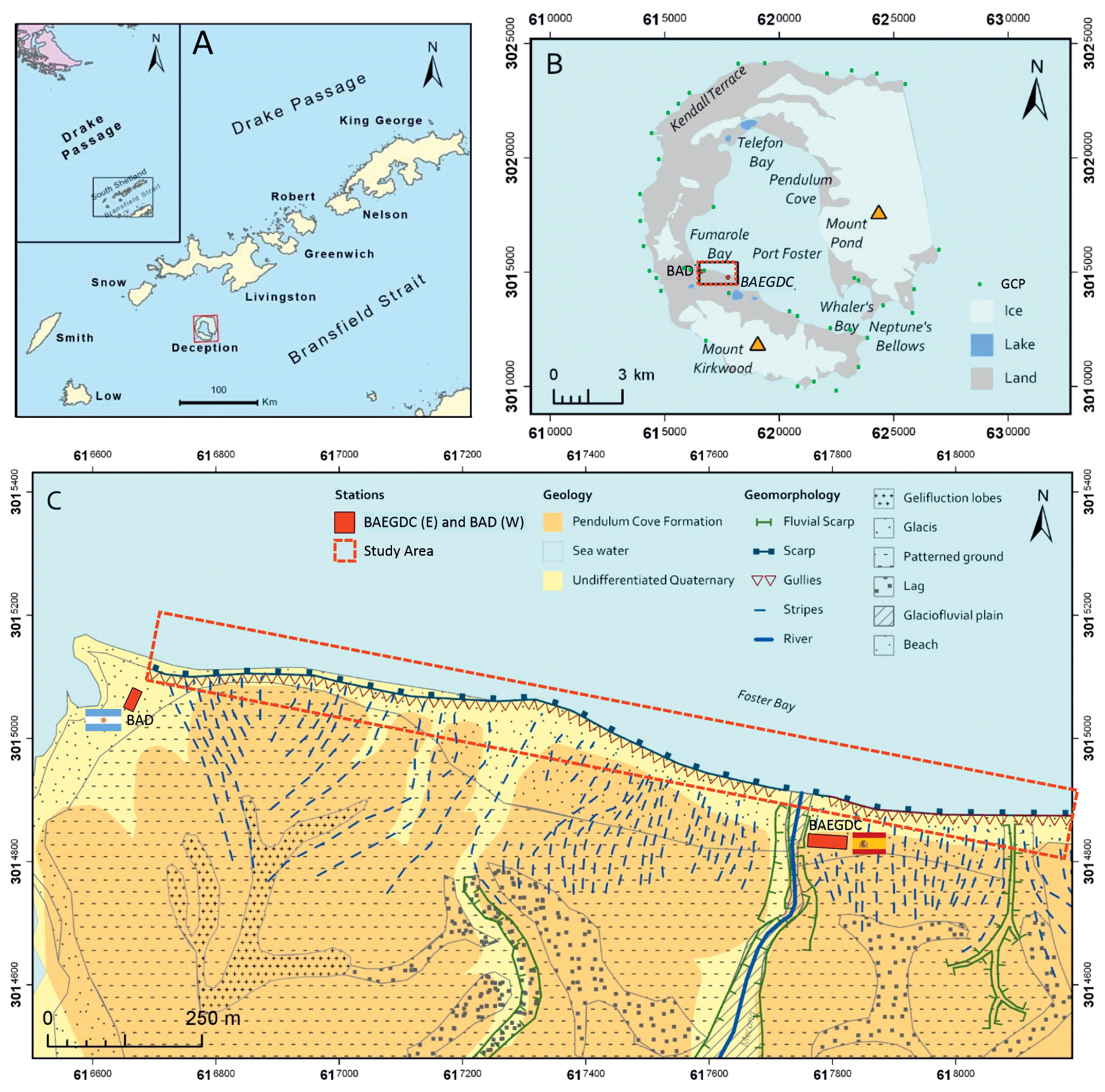
Figure 1 (a) Location of study area at Deception Island (South Shetlands, Antarctica Maritime). (b) Toponyms, scientific stations and main ice, water and land extents distribution. (c) Detailed geomorphology of the cliffed coastal area between Argentinean (BAD) and Spanish (BAEGDC) scientific Antarctic stations in this study (modified from Geological Map of Deception Island in Smellie, 2002, Geomorphological Map of Deception Island in Goyanes, 2015, and de Pablo et al., 2017). Coordinate system UTM WGS84, zone 20S, EPSG:32720.

The island's geomorphology has been shaped by intense volcanic activity, most notably a caldera collapse approximately 3980 years ago, following a VEI-6 eruption (Antoniades et al., 2018). Volcanic activity persisted over subsequent centuries, with notable eruptions in 1842, 1912, 1917, 1967, 1969, and 1970, altering the morphology of both the inner and outer coastlines (Prates et al., 2023). The resulting terrain includes steep caldera walls, glacier-capped peaks such as Mount Pond (539 m) and Mount Kirkwood (452 m) (Fig. 1b), and a diverse array of volcanic landforms, including tephra-covered slopes, pyroclastic deposits, and coastal escarpments. The study area, located between the BAD and BAEGC Antarctic Bases, is notable for its abrupt geomorphic transitions and highly variable cliff morphology (Fig. 1c).

The climate of Deception Island is classified as cold maritime polar (Cfc) or tundra (ET) (Peel et al., 2007) under the Köppen (1918) system, but is locally affected by volcanically induced geothermal flux, particularly within the caldera's interior zones (King and Turner, 1997; Caselli et al., 2002; Prieto-Ballesteros et al., 2012). Permafrost is widespread, though patchily distributed where geothermal heating and marine-air interactions elevate ground temperatures. These anomalies contribute to the formation of thermal taliks and localised areas of saline, unfrozen ground or cryopegs (de Pablo et al., 2017, 2020).

Since the mid-20th century, the region has experienced accelerated warming. Between 1951 and 2011, the western Antarctic Peninsula recorded a mean temperature increase of 0.54 °C per decade (Turner et al., 2014). Recent data (2005–2021) show annual averages of −1.1 °C, with maximum and minimum extremes of 12.7 and −22.5 °C, respectively. In contrast, temperatures in the mid-20th century (1948–1967) averaged −2.9 °C. Future climate models project a southward shift of the near-surface zero isotherm at approximately 23.9 km per decade (González-Herrero et al., 2024), which, in combination with higher rainfall and decreasing snow persistence, is expected to destabilise the permafrost and intensify coastal erosion.

Marine processes also play a significant role in shaping the island's coastal morphology. The inner bay includes beaches, minor bays, inlets (e.g., Pendulum Cove, Stancomb Cove, Telefon Bay, Fumarole Bay, Whalers Bay), and seasonal river mouths, shaped by rocky headlands (Fig. 1b). Tidal dynamics are complex, with a mixed semi-diurnal regime influenced by primary tidal constituents M2, S2, O1, and K1. Seasonal tidal ranges vary between 0.8 and 2.7 m, with meteorological tides adding up to 0.7 m during storm events (Vidal et al., 2012; Antelo et al., 2015; Figueiredo et al., 2018). Wave energy within Port Foster is modulated by a 6.5 km fetch, producing significant wave heights up to about 1.2 m, with observed breaker-zone heights of about 0.9 m and run-up levels of 0.5 m (Caballero-Martínez, 2023). These hydrodynamic forces contribute to the weathering and mechanical undercutting notch of cliff bases, particularly in unconsolidated sections. The outer coastline, in contrast, is dominated by the Outer Coast Tuff Formation, with steep volcanic cliffs several tens of metres thick, incised by glacial action and exposed to open sea conditions (Martí et al., 2013; Hopfenblatt et al., 2022). Small pocket beaches have formed at the base of these cliffs, often inaccessible except by boat, highlighting the erosional complexity of the island's exterior margins shaped by regional marine dynamics.

The selected 1.5 km bluff segment between BAD and BAEGC exhibits a substrate that includes both lithified and non-lithified pyroclastic materials, unconsolidated heterometric tephra, such as ash, lapilli, and scattered larger pyroclasts, making the terrain especially prone to rain-induced surface runoff and wave attack (Fig. 1c). The study site is lithologically characterised by the Pendulum Cove Formation, composed of post-caldera pyroclastic flows and ashfall deposits, with nearshore surfaces overlaid by the undifferentiated Quaternary formation, formed through remobilisation by solifluction and fluvial processes (Smellie, 2002). Lithologically, the material consists of poorly graded silty sands with variable grain sizes, from fine ash to bomb-sized lapilli fragments (ASTM, 2000). The vertical stratigraphy is organised into three geotechnical units (GUs): (i) the active layer (GU-AL) is 0.3–0.9 m thick in summer, with an average temperature of −0.5 °C (de Pablo et al., 2015, 2017); (ii) beneath it, the permafrost unit (GU-PF) extends from 2.5–9 m, remaining perennially cryotic (Vieira et al., 2008; Ramos et al., 2017); (iii) the subpermafrost unit (GU-ST) contains saturated or unfrozen material, often underlain by cryopeg zones, where salinity prevents freezing (González-Posadas et al., 2022).

While BAD is located on a beach, BAEGC sits on a raised on the plateau back side of the coastal bluff with a fronting beach, transitioning eastward into a more pronounced cliff shape (Paredes et al., 2021). The cliff rises gradually from west to east between the BAD and the mouth of the Mekong River, reaching a height of between 5.5 and 6 m, which remains almost constant. The cliff is between 2 and 2.5 m high from the right bank of the Mekong River to the eastern boundary of the study area, with a section of approximately 3 m on the platform where the BAEGC is located. The northern orientation of most of the bluff increases exposure to solar radiation, while the eastern sector (N88E) lies downwind of prevailing south-westerly winds, enhancing aeolian and moisture flux. The cliff base shows signs of active erosion through thermoerosional niches and shallow gullies, attributed to ephemeral summer meltwater runoff and suffusion-driven sediment transport, forming ephemeral washout cones that are rapidly reworked by wave action (López-Martínez et al., 2012; González-Posadas, 2019).

On the ground, surface temperatures fluctuate seasonally from 5 °C in summer to −5 °C in winter, with more intense variability near anthropogenically altered zones. The mean annual temperature of the upper 0.6 m remains near −0.5 °C, rendering the underlying permafrost particularly sensitive to climatic and mechanical disturbance (Streletskiy, 2021). During winter, frozen surfaces impede water flow, while in summer, snowmelt, rainfall, and anthropogenic heat flux promote active-layer deepening, slope instability, mudflows, and gully formation (López-Martínez et al., 2016) – all of which compound coastal erosion. These processes reflect a dynamic feedback between atmospheric warming, surface hydrology, and marine energy, which together contribute to the destabilisation of the cliff face.

3 Multi-temporal imagery

Various cartographic representations of the island have been created at different scales using different geodetic systems and projections (Prates et al., 2023). This has made it difficult to accurately assess temporal changes in the island's terrestrial features. Characterising potential changes in coastal dynamics requires a multi-temporal database. Sets of images from historical flights, satellite optical images and current SAR images have been used to extract the catalogue of the historical, recent and present inner coastline south-west of Port Foster. Each set is pre-processed for georeferencing, orthorectification and mosaicking.

3.1 Archive aerial imagery

Adverse meteorological conditions and operational constraints have historically limited aerial photographic missions over Deception Island. Only four historic aerial flights – conducted in 1956, 1968, 1979, and 1986 – are available, and all have been incorporated into this work (Table 1).

Table 1 Characteristics of archival aerial image acquisition from historic flights.

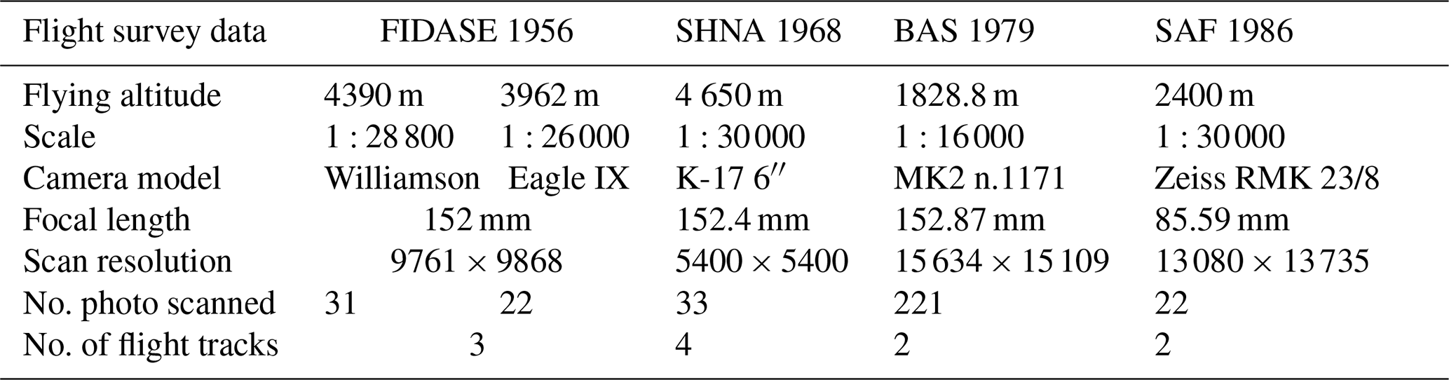
The earliest dataset was produced by the Falkland Islands Dependencies Aerial Survey Expedition (FIDASE) in December 1956. This mission aimed to systematically photograph the island vertically (Mott, 1986), using a Williamson Eagle IX camera with a 152 mm focal length and a Ross 6^′′ lens. The imagery was captured at altitudes of 3962 and 4390 m with scales of 1:26 000 (17 December 1956) and 1:28 800 (19 December 1956) respectively (Brecher, 1975). Exposure times ranged from $\mathrm{1}/\mathrm{200}-\mathrm{1}/\mathrm{50}\mathrm{s}$, and image sets consisted of two overlapping (60 % longitudinal and 30 % a lateral overlaps) series with 31 and 22 photographs. Eight astronomically triangulated control points and the proximity of nearby South Shetland Islands provided geodetic support for the mission. Scanned at 1016 dpi (10 002×10 002 pixels), the dataset has facilitated stereo-photogrammetric restitution of otherwise inaccessible regions of the Antarctic Peninsula (USGS EarthExplorer: https://earthexplorer.usgs.gov/, last accesed: 1 April 2026).

A second flight, undertaken by the Argentine Navy on 21 January 1968, followed significant volcanic activity in December 1967. The mission, executed by the Argentine Hydrographic Service (SHNA) was conducted at 4500 m with a 1:30 000 scale. 33 images were acquired across four passes (60 % longitudinal and 20 % a lateral overlaps). Despite its historical value, the scanned non-photogrammetric resolution (5400×5400 pixels at 96 dpi) and absence of precise calibration parameters posed additional processing challenges.

The third mission, led by the British Antarctic Survey (BAS) on 7 March 1979, markedly differed from the others by operating at a much lower altitude of 1828.8 m. A total of 221 images were acquired (124, RN 139/1737 RN 4/79 and 97, 1360/1737 RN5/79) from a Royal Navy helicopter using an F49 MK2 camera with a 152.87 mm focal length. High-resolution scanning (15 634×15 109 pixels at 1600 dpi) enabled accurate surface reconstructions. This set offered the finest detail among the historical flight and was key to resolving morphodynamic nuances at bluff scale.

The last historical imagery set stems from a 1986 campaign by the Chilean Air Force's Aerial Photogrammetric Service (SAF). This mission had two passes (eight images on 14 January and fourteen on 21 December), and covered the island's eastern and western sectors at a 1:30 000 scale. The used digital images have a horizontal and vertical resolution of 1400 dpi. However, disparities in acquisition dates and limited ground control in the eastern sector affected georeferencing accuracy.

3.2 Satellite imagery

To bridge the 15 year gap between the 1986 aerial mission and the emergence of high-resolution satellite imagery, eight optical satellite images (2001–2013) were integrated into the dataset. Images from the IKONOS-2, GeoEye-1, and WorldView-2 platforms were downloaded (⁺ images in Table 2) from Google Earth Pro (Google: https://www.google.es/intl/es/earth/versions/, last accessed: 1 June 2025) with cloud cover below 40 %, removing the elevation effect (assuming a value of 0.01 for the parameter representing the amplification of the effect of terrain elevation), and using maximum available resolution 8 K UHD (8192×4027 pixels). The Google Earth server allows users to download images with a resampling that alters the spatial resolution of the images (from GSD to GSD^d in Table 2) compared to the originals. The QuickBird-2 image was originally acquired (©DigitalGlobe 21 January 2003 Catalog ID 101001000192E800 with panchromatic 0.68 and 2.71 m multispectral resolutions) and selected as the ground base for georeferencing all other satellite scenes because of its optimal clarity and 0 % of cloud coverage.

Table 2 Parameters of satellite images from the recent past: Date: date of acquisition, CC: cloud cover in the full image, GSD: maximum ground sampling distance (m) in the original image, GSD^d: pixel size (m) in downloaded image after resampling from Google Earth Pro, ION: image tilt, SE: sun elevation/orbit. ⁺ Image ©2025 Maxar Technologies, * Image U.S. Geological Survey, ¹ ©DigitalGlobe,
² ©Hisdesat Servicios Estratégicos S.A.

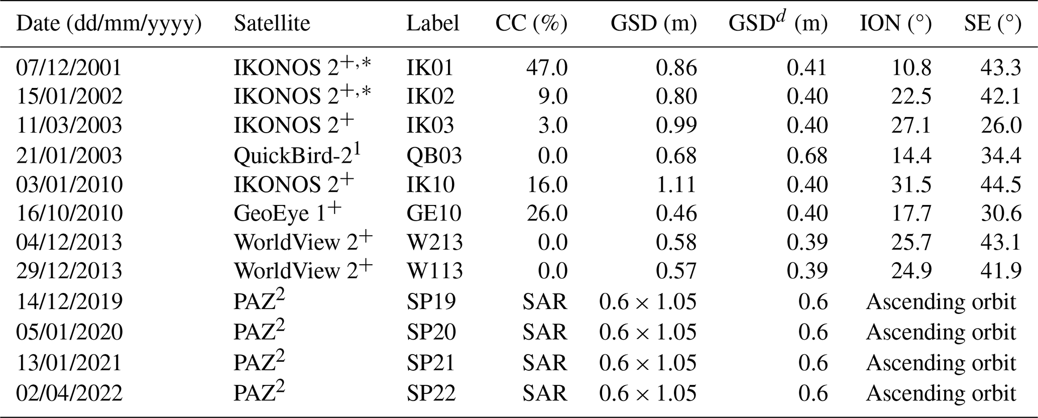
To supplement optical datasets, four synthetic-aperture radar (SAR) images were acquired and incorporated from the PAZ (©Hisdesat Servicios Estratégicos S.A.) mission between 2019–2022. Acquired hight-resolution spotlight SAR images in ascending orbital passes, these X-band SAR products offered a resolution of 0.6 m×1.05 m per pixel. SAR image geolocation errors were derived directly from PAZ documentation (Bonilla et al., 2024).

Following pre-processing, all raster layers were harmonised spatially within a GIS framework. This multitemporal geospatial foundation formed the basis for delineating shoreline reference lines (Ankrah et al., 2022), which are analysed further using the SCA-TBM methods described in subsequent sections.

4 Methods

This study employed a quantitative approach to SCA-TBM for evaluating cliff-top retreat. The objective was to determine and model the net spatial displacement of the bluff top through temporal analysis of georeferenced imagery. This approach enabled the calibration of both linear and non-linear regression models of erosion behaviour across defined sections of the study area. Historical aerial photographs (Table 1) and more recent satellite imagery (Table 2), both optical and SAR-based, were orthorectified and spatially aligned using a unified ground control framework based on the panchromatic QuickBird-2 image dated 21 January 2003.

A GIS-based workflow was implemented to digitise the cliff-top as a reference line (Himmelstoss et al., 2006) and its associated positional uncertainty for each orthorectified image. This dataset spans a 66 year time series from 1956–2022. The resulting reference lines were discretised via a transect system anchored to a fixed baseline, allowing calculation of shoreline change metrics, uncertainty-weighted rates of change, and derivation of morphodynamic insights from fitted regression models.

4.1 Photogrammetric pre-processing and image georeferencing

A photogrammetric restitution process was undertaken to construct orthoimage mosaics from scanned images of the four archival aerial flights (Table 1). The increased computational efficiency and capabilities of Structure-from-Motion (SfM) and Multi-View Stereo (MvS) techniques have revolutionised photogrammetric processing, offering viable alternatives to traditional stereo restitution (Cook, 2017). This method facilitates the reconstruction of dense point clouds by identifying homologous features across multiple overlapping images and calculating their spatial coordinates relative to the camera reference frame.

The full 3D reconstruction pipeline requires knowledge of ground control points (GCPs) and camera centre (CC) positions within a consistent reference system. Outputs include a dense point cloud (DPC), a triangulated irregular network (TIN), a digital elevation model (DEM), and a high-resolution orthorectified mosaic image (HROM). However, the application of SfM-MvS to historical aerial imagery in polar environments presents numerous technical challenges (i.e. Riquelme et al., 2019). These include missing camera calibration data (e.g. FIDASE 1956), eroded or absence of fiducial marks (e.g. SHNA 1968, BAS 1979, SAF 1986), high flight altitudes, large image scales, and scanning artefacts or surface damage.

Despite these limitations, a refined SfM-MvS workflow was implemented using Agisoft Metashape PhotoScan Professional (v2.1.3, Agisoft LLC, 2024, St. Petersburg, Russia), based on the protocols proposed by Over et al. (2021) to overcome the differences and quality criteria to get the DPCs, TINs and HROMs (Child et al., 2021; Prates and Vieira, 2023; North and Barrows, 2024, among others). The optimisation focused on minimising three main sources of error in the outputs: Uncertainty Reconstruction (UR), Projection Precision (PP), and Reprojection Error (RE). Acceptable thresholds were set as follows: UR ≤ 10, PP ≤ 10, RE ≤ 1 pixel, contingent on image quality (Paredes et al., 2021). A total of 37 stable GCPs were selected for this process. These were identified both in the historical images and in the QuickBird-2 image, primarily consisting of immobile rocky outcrops and promontories unaffected by volcanic or cryospheric changes since 1956. GCPs were georeferenced using WGS84 – UTM20S (EPSG:32720), providing positional consistency across image sets and contributing to the elevation restitution of each orthophoto mosaic (Prates et al., 2023). Each historical flight was processed individually, generating TIN, DTM, and HROM outputs for subsequent analysis.

All historical aerial images were processed in Agisoft Metashape to generate orthorectified mosaics, enabling their integration into a unified geospatial framework (WGS84 – UTM 20S, EPSG::32720). Ground Control Points (GCPs) were visually identified across stable features – such as rocky promontories and infrastructure at BAD and BAGC – and used to correct each flight set. Over 30 GCPs were employed per flight (Fig. 1b), ensuring sub-metre Ground Sampling Distance (GSD^k in Table 3). The resulting Root Mean Square Errors (RMSE) for these historical orthoimages ranged from 0.76–22.7 m, depending on image quality, flight characteristics, and the number and distribution of GCPs (Table 3). However, for the SAF 1986 series, which consisted of two acquisition passes taken on different dates, the georeferencing relied on only 16 GCPs for the western half, resulting in higher RMSE values, particularly in the western half.

Table 3 Quality indexes of multitemporal geoinformation after processing: ⁺ photogrammetrically derived orthophoto from archival images, ^* georeferencing for optical satellital images and ^x RDTC correction for PAZ images.

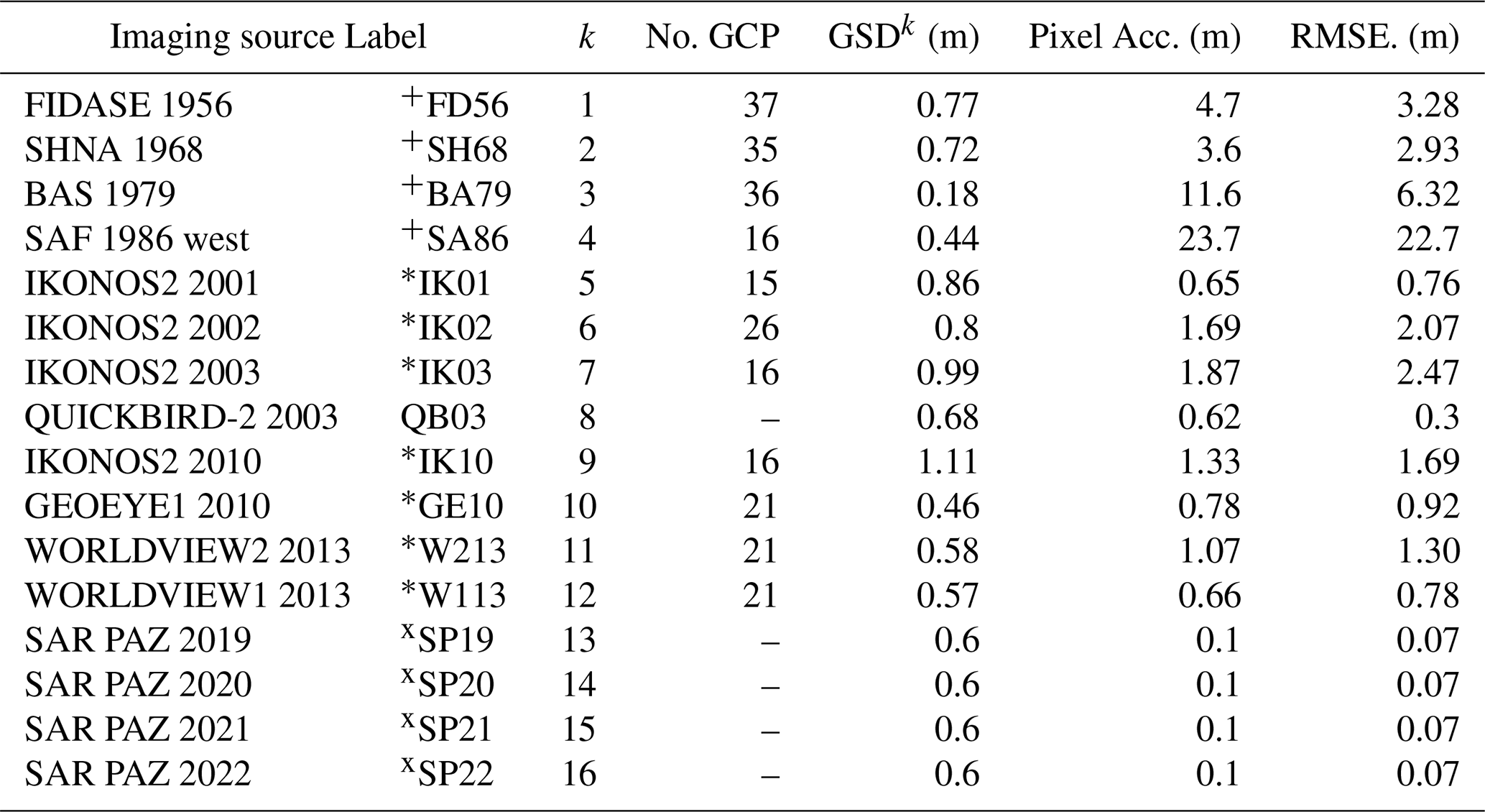
Satellite images (2001–2013), although ortho-projected, lacked spatial referencing and were therefore georeferenced using the 2003 QuickBird-2 image as a reference. Between 15 and 21 GCPs were placed on persistent geomorphic features – mainly rocky outcrops and structural landmarks at the research stations – to conduct geometric correction via second-order polynomial transformation. Resulting RMSEs ranged from 0.3–2.5 m, with all images maintaining GSD values below 1 m, ensuring suitable spatial resolution for cliff-top identification.

The photogrammetric processing of all imagery – historic aerial and optical satellite – was performed within a coherent spatial framework. This alignment facilitated consistent shoreline reference line digitisation and uncertainty band delineation across the 66 year image sequence. The resulting high-resolution, georeferenced datasets form the analytical basis for the subsequent shoreline change analysis and regression modelling.

For the purposes of this study, it has been established that, despite the downloaded images having been resampled by Google Earth Pro, resulting in a lower GSD^d, the GSD^k will be taken as the GSD of the source image (Table 3) for the effects of associated uncertainty. Additionally, in the absence of embedded spatial metadata in satellite optical images downloaded from Google Earth Pro, georeferencing into the common geospatial framework (WGS84 – UTM 20S, EPSG::32720) was necessary. The geographical area covered by each satellite image (slightly larger than that shown in Fig. 1c, see Supplement) was manually rectified against the QuickBird-2 reference image using a map-to-map georeferencing strategy within a GIS environment. Several GCPs were selected from persistent landscape features and built infrastructure (e.g. buildings at BAD and BAEGC), ensuring uniform spatial distribution and optimising georeferencing accuracy. Variations in image characteristics (lighting, contrast, resolution) meant that not all geometric control points (GCPs) could be detected in all satellite images. A minimum of ten GCPs per image was employed, and spatial accuracy of the georeferenced area was quantified using root mean square error (RMSE in Table 3) metrics using a second order polynomial transformation (the satellite images and the GCPs used for their rectification can be found in the Supplement).

In contrast, SAR images from the PAZ mission do not require georeferencing, as they are provided with intrinsic geolocation metadata. Nonetheless, orthorectification is essential to correct geometric distortions introduced by sensor tilt and terrain variability. Without such corrections, image displacement can compromise the spatial accuracy of morphometric analyses, particularly in topographically diverse coastal environments. To correct terrain deformation according to the antenna orientation, each SAR image, the Range Doppler Terrain Correction (RDTC) algorithm (Small and Schubert, 2022) was applied using the SNAP toolbox (ESA, 2024), with elevation data from the REMA DEM (Howat et al., 2019). The RDTC algorithm modifies the native GSD of the SAR-PAZ image. By default, SNAP resamples the image to the resolution of the Digital Elevation Model (DEM) used (in our case, the REMA at ∼8 m), although the desired GSD has been manually configured in the processor parameters to maintain it at 0.6 m. This ensured geocoded rectification of all SAR images from 2019–2022, yielding terrain-adjusted products suitable for integration into the time series.

4.2 Extraction of Reference Lines and their Uncertainties

A valid SCA requires a reference line that can be clearly identified in each of the multitemporal images used (Boak and Turner, 2005). For this study, the reference line was manually interpreted from each image in a GIS environment and positioned along the bluff top, where visual evidence of geomorphic change was most reliably captured. The visibility of this edge is typically more consistent across the diverse image catalogue than that of the cliff base, which is often obscured by shadow or backshore debris. The decision to trace the top or erosion scarps, rather than the foot, of the coastal bluff was influenced by the limitations of available data: DEMs derived from historical flights lack the necessary resolution, and no full temporal DEM sequence exists to support automatic tracing of slope breaks (Young et al., 2009; Farquharson et al., 2018). Figure 2 presents the conceptual model used for reference line delineation. On this model, the reference line (yellow) is traced along the visible ridge of the bluff on a consistent digitising plane. The associated uncertainty band (between the red and green lines) accounts for visual ambiguity and potential digitisation error. The red line represents the perceived start of the bluff's face when viewed from above, while the green line marks the transition into the inland plain or attenuated slopes. Furthermore, the visual conditions – affected by sun angle, shadow length, and surface contrast – often render the base of the bluff indistinct, while the top maintains relatively stronger visual continuity across all imagery.

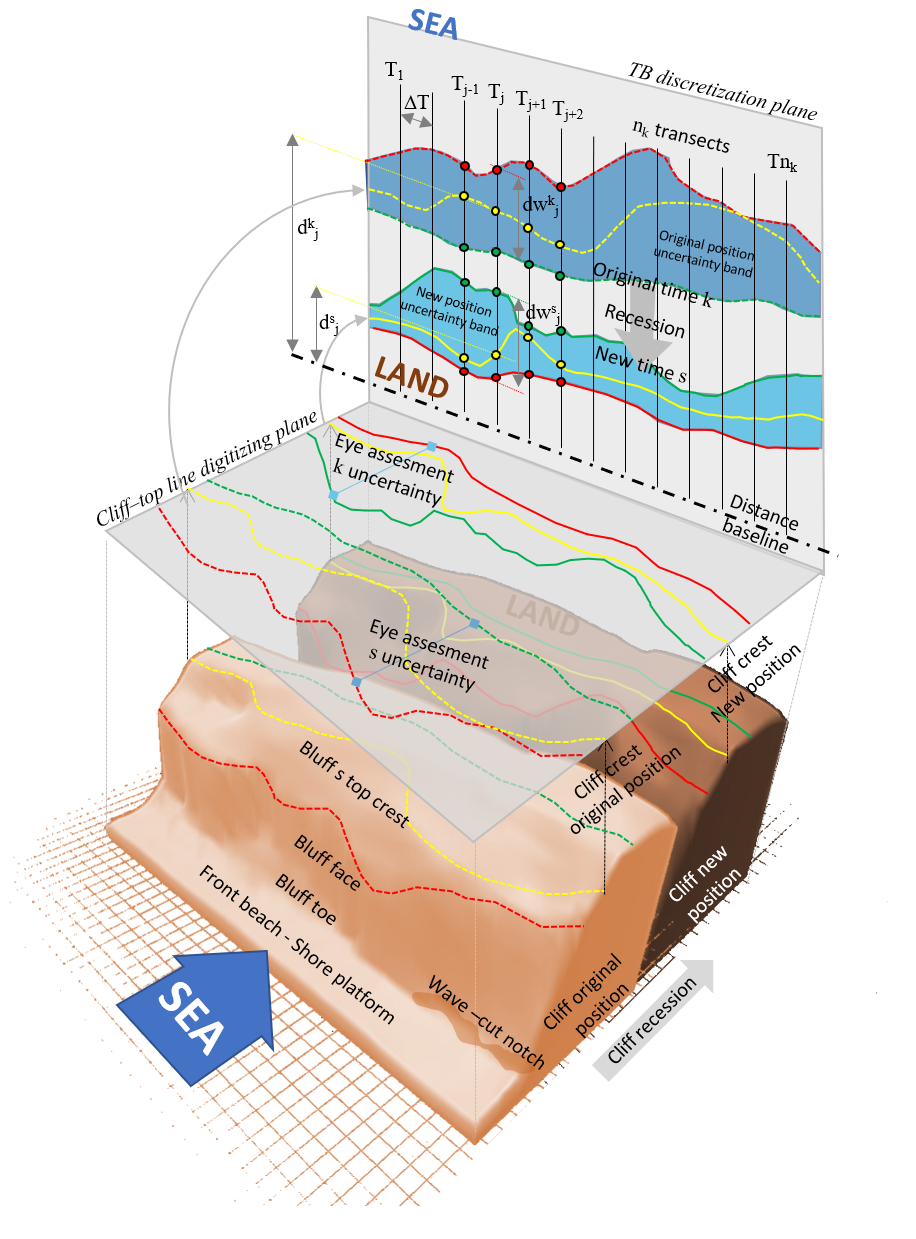
Figure 2 Block diagram of the coastal bluff on which the reference lines and their uncertainty bands are delineated (in the digitising plane), and the TBM is applied for their discretisation (in the discretisation plane).

The wide heterogeneity of image types and qualities (Tables 1 and 2) ruled out the use of automated edge detection or segmentation techniques across the full dataset. Semi-automatic tracing, although promising in controlled conditions (Tsiakos and Chalkias, 2023; Philipp et al., 2022; Kazhukalo et al., 2023; Tsai, 2024; Scala et al., 2024; Lu et al., 2024), was impractical due to the inconsistent resolution, contrast, and illumination across the 66 year imagery archive. Instead, the reference line was manually traced by a single operator to ensure consistency. To aid this visual interpretation, histogram equalisation (HE) technique were applied to each image, improving contrast in colour channels and facilitating the identification of geomorphic markers relevant to the top of the bluff. HE is an effective and well-established method of indirect contrast enhancement, whereby the image histogram is modified (see, for example, Vukadinov et al., 2017). The combination of histogram equalisation across different colour ranges serves to highlight certain morphological changes and other coastal features, including the band in which it is visually located (the sth ridge of the bluff) and the manual tracing of the sought ridge (Fig. 2, yellow line) on a common digitising plane.

Errors in the precise placement of reference lines stem from several factors: (1) resolution limitations of older imagery; (2) diffuse morphological expression of the bluff top; (3) variable viewing altitudes and angles; and (4) reduced contrast in snow-covered or shadowed areas (Warnasuriya et al., 2020). These sources of error were addressed by plotting an uncertainty band around each digitised top line. This band, manually delineated (Fig. 2, band between the red and green lines), reflects the operator's judgement of the plausible spatial range within which the top might reasonably lie based on visual and morphological cues. This procedure was repeated for each image date, producing a time-series catalogue of top reference lines (e.g. kth bluff edge) and associated uncertainty bands (e.g. kth uncertainty band). These features were projected in zone 20S (EPSG::32720) and stored as polygons within a GIS-based geodatabase for further analysis.

To quantify the uncertainty associated with each line, the width of the band between the red and green boundaries was measured for every digitised transect. These distances were calculated for the n^k j-points where the reference lines were discretised (yellow dots in Fig. 2) using the TBM and uncertainty band boundaries (red and green dots in Fig. 2). This uncertainty width, denoted as ${\text{dw}}_j^k$, was later used in the statistical treatment of the distance-time datasets. The spatial variation in band width across transects and time was assessed to inform weighting strategies in subsequent shoreline change modelling.

The cumulative effect of these uncertainties – arising from kth-image resolution (GSD^k), photogrammetric orthorectification (GE^k1), georeferencing errors (GE^k2), and manual digitisation ($d_j^k$) – was integrated into a total uncertainty metric ${\text{Et}}_j^k$, calculated using the following root sum square formulation (Hapke et al., 2011; Ruggiero et al., 2013):

The cumulative effect of these uncertainties – arising from kth-image pixel resolution GSD^k, photogrammetric orthorectification ${\text{GE}}_{\mathrm{1}}^k$ only for aerial imagery (pixel accuracy in Table 3), georeferencing errors ${\text{GE}}_{\mathrm{2}}^k$ (RMSE in Table 3), and manual digitising uncertainty such as the digitisation bandwidth (Fig. 2) in the jth transect (${\text{dw}}_j^k$)–was integrated into a total positional uncertainty metric ${\text{Et}}_j^k$ for each jth transect, calculated using the following root sum square formulation (Crowell et al., 1991; Fletcher et al., 2003):

$$\begin{array}{}\text{(1)}& {\text{Et}}_j^k={\left(({\text{GSD}}^k{)}^{\mathrm{2}}+{\left({\text{GE}}_{\mathrm{1}}^k\right)}^{\mathrm{2}}+{\left({\text{GE}}_{\mathrm{2}}^k\right)}^{\mathrm{2}}+{\left({\text{dw}}_j^k\right)}^{\mathrm{2}}\right)}^{\mathrm{1}/\mathrm{2}}\end{array}$$

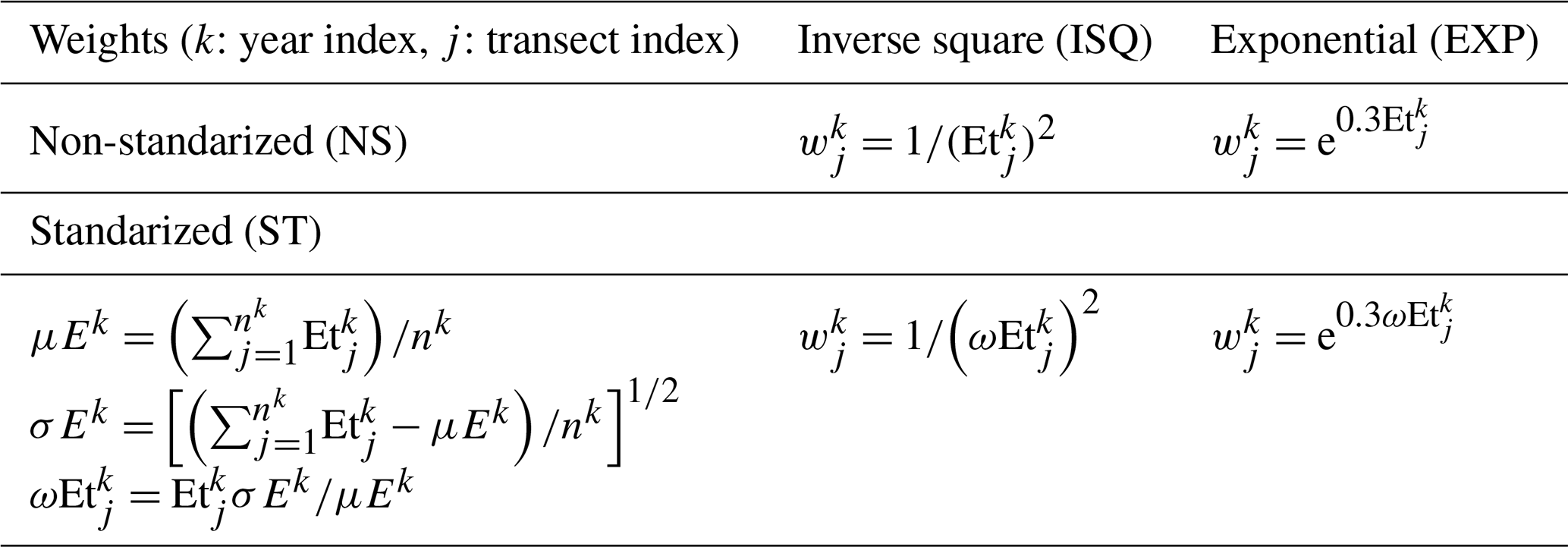
This error metric was computed for each time step k (k≡year: 1956, 1968, 1979, 1986, 2001, 2002, 2003, 2010.01, 2010.10, 2013, 2019, 2020, 2021, 2022), and transect $j=\mathrm{1},\mathrm{\dots },\text{NT},$ being NT the total number of outlined transects. Each ${\text{Et}}_j^k$ value is incorporated in the least square models within SCA by means of a weighting scheme (i.e. Genz et al., 2007). Combining the multiple sources of uncertainty in the data (Eq. 1) along NT transects, the normalized weight $W_j^k$, is calculated here according to non-standarized and standardized weighting schemes (Table 4), using:

$$\begin{array}{}\text{(2)}& W_j^k={\displaystyle \frac{w_j^k}{{\sum }_{i=\mathrm{1}}^{\text{NT}}{w}_j^k}}\end{array}$$

All extracted and weighted reference lines and uncertainties were prepared for transformation into the TBM discretisation system (Fig. 2), the subject of the following Section.

Table 4 Expressions of the weights used in this work to incorporate the multiple sources of uncertainty in the data.

4.3 Shoreline change statistics and least square regressions

The SCA was performed using Shoreline Change Statistics (SCS), assessing both linear and non-linear trends over time (Dolan et al., 1991; Fenster et al., 1993). Reference lines and their uncertainty bands were transformed into a point cloud through the Transect-Based Method (TBM), intersecting with a series of equidistant transects (T_j) spaced at 5 m intervals (Fig. 2), allowing for consistent discretisation across the coastal stretch (Warnasuriya, 2023).

The distances $d_j^k$ from each shoreline reference line to a fixed inland baseline were calculated for all time points and transects. These values were weighted by $W_j^k$ based on the total uncertainty ${\text{Et}}_j^k$ within the least square regression framework of SCS. All statistical computations were implemented in the MATLAB-based CREES software tool (Cliff Retreat Enhanced Estimation and Simulation). For each transect and time sequence, CREES computes: (i) Shoreline Change Envelope (SCE): the maximum range between recorded shorelines; (ii) Net Shoreline Movement (NSM): distance between earliest and latest shoreline positions; (iii) End Point Rate (EPR): shoreline movement over elapsed time. CREES also calculates weighted descriptive statistics, including covariance and Pearson's correlation, to evaluate the dependence between shoreline position and time, assessing the extent of linearity across each T_j transect.

Computationally, each distance-time pairs ($d_j^k$, t^k) time-series (t^k in days since an arbitrary time origin) per jth-transect was fitted using ordinary least squares (OLS) regression. To reduce the influence of outliers, robust regression was applied through reweighted least squares RWLS (Genz et al., 2007), using a minimisation criterion for weighted residuals (Rousseeuw and Leroy, 2003). Once an arbitrary model D(t) is selected accordingly to the ($d_j^k$, t^k) time-series observed behaviour, the residual sum of squares or sum of squares error (SSE_j) was minimised, for each $j=\mathrm{1},\mathrm{\dots }\text{NT}$, as follows:

$$\begin{array}{}\text{(3)}& {\text{SSE}}_j=\sum _k{W}_j^k{\left(d_j^k-D\left(t^k\right)\right)}^{\mathrm{2}}\end{array}$$

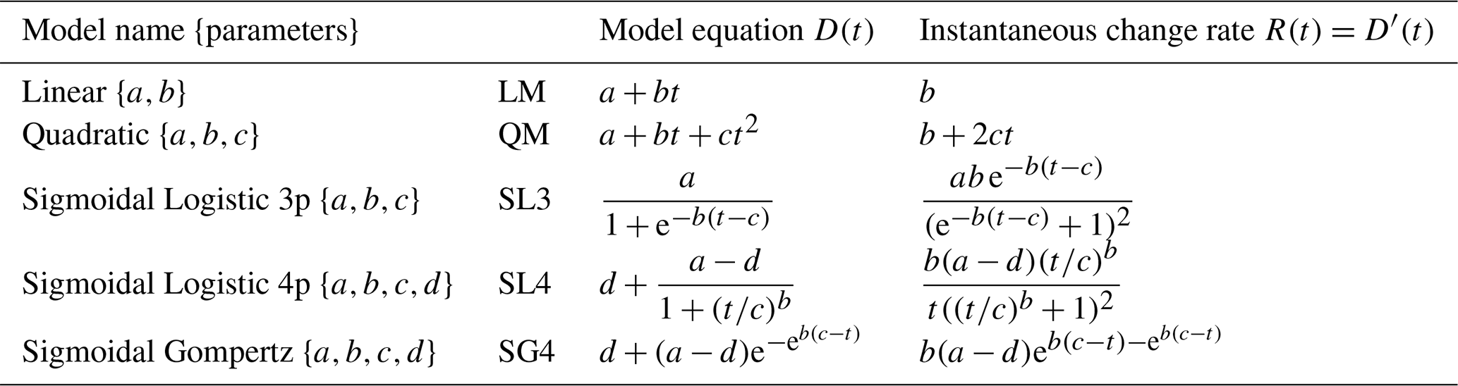
Here, model D(t) fitting included both standard linear in SCA software (Danforth and Thieler, 1992; Jackson et al., 2012; Gómez-Pazo et al., 2022, among others) and non-linear forms (Table 5). Thus, in addition to the standard linear model, second-order polynomial, logistic sigmoid, and Gompertz models were used to describe varying erosion-accretion dynamics, including potential acceleration phases (Fenster et al., 2001; Tsai, 2024). Instantaneous change rates, $R\left(t\right)=\mathrm{d}D\left(t\right)/\mathrm{d}t$, were derived from each fitted model to track temporal changes.

Model performance was evaluated here with CREES, for each fitted model (Table 5) minimizing Eq. (3), using: (i) R²: goodness of fit, (ii) STDE: standard error of estimate or RMSE, (iii) AICc: corrected Akaike information criterion, (iv) 95 % CI: confidence interval of the rate. Transect dynamics were classified into (Tsai, 2024): (i) Random: if R²<0.6 for all models, (ii) Correlated: if one model exhibited highest R² and lowest AICc and STDE. This classification supports the identification of spatial trends in coastal behaviour and enables robust interpretation of bluff evolution patterns.

Table 5 Different models used in this work for of discrete distance-time D(t) vs. t data least squares regression, and its instantaneous derived velocity R(t).

5 Results

5.1 Extraction of reference lines and shoreline change statistical analysis

Following image pre-processing, georeferencing, and correction, reference lines and uncertainty bands were manually delineated in a GIS environment. This was performed by a single trained operator using HE techniques to enhance visual contrast across RGB channels, facilitating consistent interpretation of 16 shoreline positions spanning the period 1956–2022 (Fig. 3a). Despite challenges such as snow cover and low contrast in certain image sets, the method enabled reliable delineation of the bluff edge for each date. The furthest inland and nearest coastal positions, derived from contrast differences, were used to define maximum and minimum polygons representing the uncertainty band for each reference line (Fig. 3b). The resulting polygonal bands were transformed into point datasets by the TBM, generating discrete points every 5 m across a total of 294 transects oriented approximately north–south. This resolution was considered adequate for characterising spatially heterogeneous evolution patterns while maintaining analytical tractability.

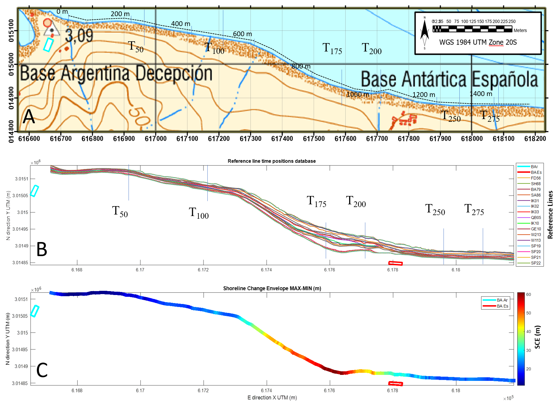
Figure 3 (a) Detail in the study area marking the distances over the coastline measured from the western boundary and three of the control transects selected in this work (T₅₀, T₁₇₅ and T₂₇₅). (b) Catalogue of 16 polygonal lines extracted from the processing of the images in the study area and their discretisation into points with TBM (points on the polylines). (c) Shoreline change envelope (SCE) between the first reference line (FIDASE 1956) and the last one (SAR PAZ 2022).

The Shoreline Change Envelope (SCE) captured the largest retreat values – up to 60 m – within the central third of the study area, particularly around the left bank of the Mekong River estuary, the only easterly-facing coastal segment (Fig. 3c). These high rates of displacement illustrate the non-homogeneous distribution in retreat intensity along the cliff crest. Conversely, cliff sections adjacent to the BAD station showed minimal change, averaging under 11 m, while much of the remaining bluff experienced shifts below 30 m. The segment fronting the BAEGC, with a mostly north-facing orientation, exhibited intermediate retreat values in the 30–40 m range.

Uncertainty analysis revealed a diverse range in the band widths ${\text{dw}}_j^k$ between the maximum and minimum line for each year. Values ranged from 1.2–39 m, the latter seen in low-contrast imagery from GE1 2010. Despite such exceptions, 90 % of the uncertainty widths were below 15 m. and interquartile ranges for most transects fell between 5 and 10 m, with a small number of outliers linked to variable image quality. No consistent spatial clustering of uncertainties was observed along the cliff, although a general temporal trend was evident – recent imagery consistently yielded narrower uncertainty bands and lower variance. This reflects improvements in resolution and sensor calibration over time.

Once integrated these uncertainties, distance-time data points were weighted according to a composite measure in Eq. (1), with normalisation applied as Eq. (2) and equations in Table 4. High-resolution, recent imagery received higher weights (closer to 1), contributing more strongly to regression analyses and statistical estimates. Earlier or lower-quality datasets with larger uncertainty bands were included but down weighted accordingly, minimising distortion in model outcomes.

Using the weighted distance-time dataset, descriptive statistical analysis was conducted across all transects. Sample covariances (Fig. 4a) and Pearson's correlation coefficients (Fig. 4b) were calculated to assess the linearity and strength of shoreline evolution over time. In all cases, both statistics were negative, confirming a general retreat trend. Pearson's correlations ranged from −0.78 to −1.0, while the weighted correlations ranged between −0.77 and −1.0, indicating improved robustness in the presence of uncertainty. However, covariances exhibited notable oscillations along the transect axis, particularly across the central third of the study area, where values approached $-\mathrm{140}\times {\mathrm{10}}^{\mathrm{3}}$. These spatial fluctuations along the cliff top suggest that erosion dynamics are not uniformly distributed and may be influenced by local geomorphological or exposure conditions. Despite incorporating differential weighting, the pattern of statistical dependence between shoreline positions and time remained broadly consistent, confirming the robustness of the SCA-TBM framework and the analytical processing applied.

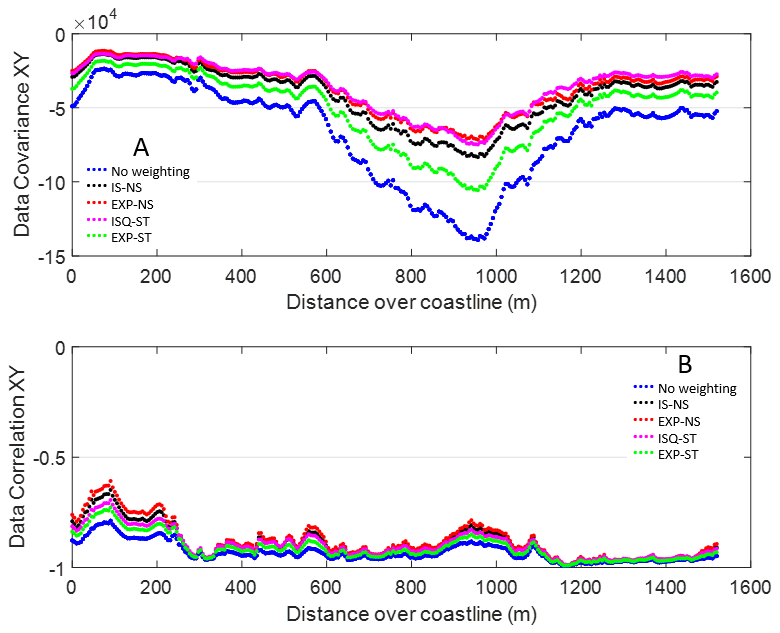
Figure 4 (a) Data Covariance and (b) Pearson's correlation coefficient related with distance travelled along the coastline from western initial point.

5.2 Regression of least square models

The application of the classical Shoreline Change Analysis (SCA) using a linear regression model (LM, Table 5) was conducted over the 294 transects across the study area. The estimated instantaneous rates of change R(t) show consistently negative slopes b<0, indicating bluff retreat. The regression-adjusted LM revealed significant spatial variability along the coastline. For instance, the distribution of distance versus time data across transects (three of them in Fig. 5a) E–W transitions from a moderately decreasing pattern (i.e. at T₅₀) with correlation $\approx -\mathrm{0.75}$, to a linear trend (i.e. at T₁₀₀) with correlation $\approx -\mathrm{0.93}$, and even stronger $\text{correlations}<-\mathrm{0.98}$ (i.e. at T₂₅₀). Despite this high negative correlation, noticeable data dispersion around the regression lines persists. Narrowing of 95 % confidence intervals towards more recent observations highlights the increasing reliability of later data linked to reduced errors.

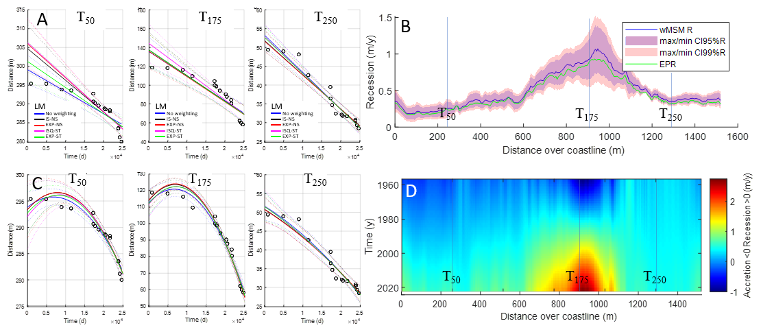
Figure 5 LM and QM regression results: (a) detail of the fitted LM to distance vs. time (days since FD56) at transects 50, 175 and 250 (solid lines) and their 95 % prediction bounds across the LM fit range (dotted curves around each linear model), applying the four weighting schemes considered in this work (Table 4) and without weighting. (b) Rate of change R (in m yr⁻¹) fitted with the ML (blue line) by least squares method (MSM) and EXP–ST weighting. Confidence intervals (CI) on R (at 99 % and 95 %) are represented around R, and the end-point rate (EPR, plotted with green line) at each transect along the study area. (c) Detail of the fitted QM to distance vs. time (days since FD56) at transects 50, 175 and 250 (solid parabolas) and their 95 % prediction intervals across the QM fit range (dotted curves around each parabolic model), applying the four weighting schemes considered in this work (Table 4) and without weighting. (d) Instantaneous rate of change R(t) map (in m yr⁻¹) fitted with the QM (R(t) in Table 5), with weighting EXP–ST, along the time interval [1956, 2022] for each jth transect (j=1..) along the study area. The location of the transects T₅₀, T₁₇₅, T₂₅₀ used are marked in (b, d).

The R(t) from LM outputs clearly and regardless of the weighting scheme used in the regression identify three distinct spatial zones. The R(t) results presented here (Fig. 5b) are using the EXP–ST scheme (the results obtained for the four weighting schemes and for the unweighted case are included in the Supplement). The western segment (T₁−T₁₂₅, along shore range 0–600 m) exhibits modest retreat rates ($b<\mathrm{0.5}\mathrm{m}{\mathrm{yr}}^{-\mathrm{1}}$) with values between 0.17 to $\mathrm{0.4}\pm \mathrm{0.12}\mathrm{m}{\mathrm{yr}}^{-\mathrm{1}}$, with a mean of 0.25 m yr⁻¹. These rates closely match the EPR, with narrow 95 % and 99 % confidence intervals. Residuals are tightly confined within ±2 m, and interquartile ranges rarely exceed 1 m. The central segment (T₁₂₅−T₂₁₅, along shore 600–1100 m) shows the highest retreat rates ($\mathrm{0.4}\pm \mathrm{0.1}-\mathrm{1}\pm \mathrm{0.4}\mathrm{m}{\mathrm{yr}}^{-\mathrm{1}}$), especially near the mouth of the Mekong River. This region also exhibits larger 90 % and 95 % confidence intervals and the highest residuals, ranging ±4 m, with interquartile spreads of about 3 m. The easternmost segment (T₂₁₅−T₂₉₄, along shore range 1100–1500 m) features intermediate retreat rates ($b\approx \mathrm{0.5}\pm \mathrm{0.1}\mathrm{m}{\mathrm{yr}}^{-\mathrm{1}}$), with smaller uncertainties and interquartile ranges around 0.5 m.

The quadratic model (QM) regression, independent of weighting, appear to be improved. These results suggest the possibility of temporally non-linear accretion/erosion behaviour. However, QM produce initial positive rates R(t)>0 (up to 1 m yr⁻¹), notably at T₅₀ and T₁₇₅, before transitioning to negative rates (Fig. 5c). These trends highlight a maximum in shoreline position D(t) around 2000, after which consistent change rates accelerates until 2023, reaching $-\mathrm{3}\mathrm{m}{\mathrm{yr}}^{-\mathrm{1}}$ at T₁₇₅ and $-\mathrm{0.45}\mathrm{m}{\mathrm{yr}}^{-\mathrm{1}}$ at T₂₅₀ on average. Space–time map of $R\left(t\right)=b+\mathrm{2}ct$, representing the slope R(t) space–time variability, confirm this zonal structure (Fig. 5d). This R(t) results are using the EXP–ST scheme (the space–time maps obtained for the four weighting schemes and for the unweighted case are included in the Supplement). The first zone (T₁−T₁₂₅) saw $R\left(t\right)<\mathrm{1}\mathrm{m}{\mathrm{yr}}^{-\mathrm{1}}$ by 2023, with earlier acceleration. Despite low sensitivity to weighting, this zone shows the widest 95 % confidence intervals (up to 14 m), which narrow markedly over time. The second zone (T₁₂₅−T₂₁₀) is marked by retreat rates close to 2.5 m yr⁻¹ by 2023. The third zone (T₂₁₀−T₂₉₄) displays persistent $R\left(t\right)<\mathrm{0.5}\mathrm{m}{\mathrm{yr}}^{-\mathrm{1}}$, with minimal temporal variation.

Sigmoidal regression models – SL3, SL4, and SG4 – although they are more sensitive to weighting, as seen at T₂₅₀ and T₂₇₅ improve the fits respect to LM and QM (Fig. 6a–i). Here, in unweighted fits, they failed to capture acceleration phases accurately, while weighted fits exhibited steeper sigmoid curves. All three sigmoidal models (SL3, SL4, SG4) successfully captured monotonic decreases in shoreline position R(t)≤0 in the transects T₅₀ to T₁₇₅, without sign reversals. The three sigmoidal models are capable of fitting a portion of the sigmoid, demonstrating a monotonic decreasing behaviour (R(t)≤0), in the T₅₀ to T₁₇₅, with no sign changing sections (R(t)>0), as observed in the QM. However, the SL3 model could not model elevated retreat rates ($\left|R\right(t\left)\right|>\mathrm{0.35}\mathrm{m}{\mathrm{yr}}^{-\mathrm{1}}$) effectively, often reverting to a quasi-linear trend, resembling the LM.

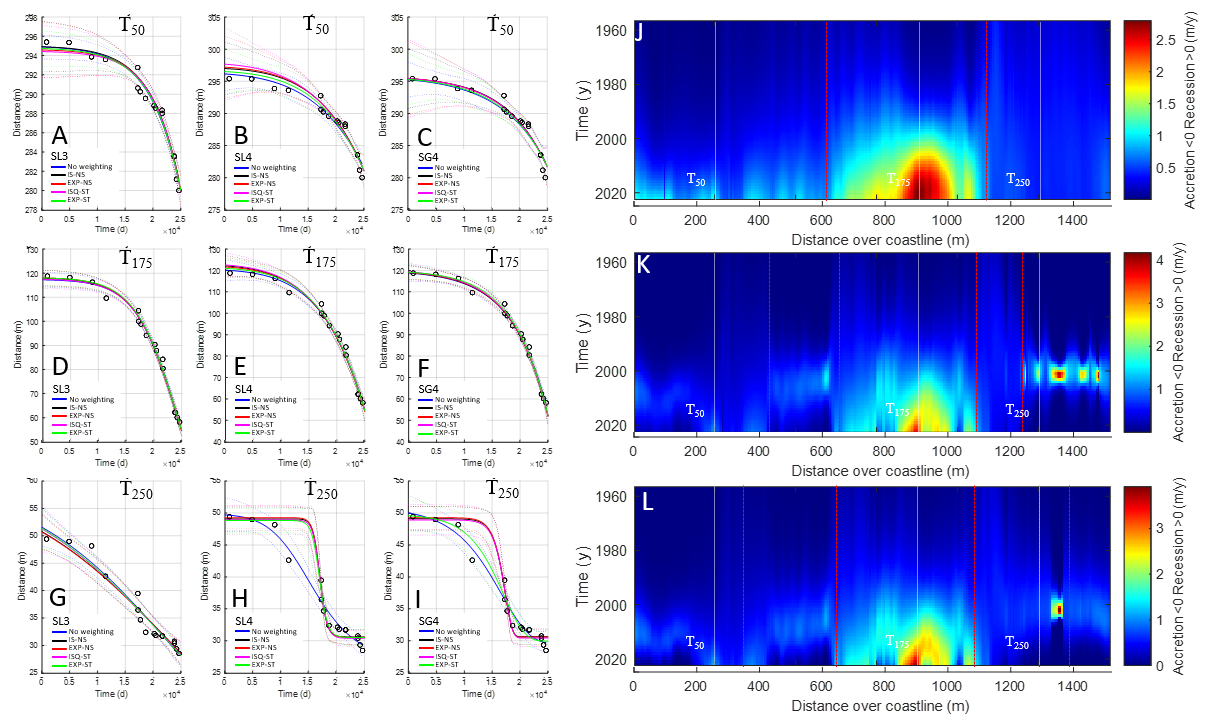
Figure 6 (a–i) Sigmoidal regression results from SL3, SL4 and SG4 models to distance vs. time (days since FD56) at control transects 50, 175 and 250 (solid curves) with their 95 % prediction intervals across the fit range (dotted curves around each sigmoidal model), applying the four weighting schemes considered in this work (Table 4) and without weighting. Instantaneous rate of change R(t) space–time map (in m yr⁻¹) fitted with the (j) SL3, (k) SL4 and (l) SG4, with weighting EXP–ST. along the time interval [1956, 2022] for each jth transect (j=1..) in the study area, The detected changes in R(t) dynamics, along the study area, are marked with red dashed lines on each map, see their explanation in the main text.

Across the full set of transects, a generalised trend of increasing retreat velocity (R(t)<0) is observed over the course of the study, spanning all transects and years, in contrast to the QM model, which exhibits no time sections with R(t)>0. The SL3 model produced three distinct spatial behaviours (Fig. 6j): (1) western sector (T₁−T₁₂₀) with accelerating erosion up to 1 m yr⁻¹; (2) central sector (T₁₂₀−T₂₂₀) with acceleration exceeding 2.5 m yr⁻¹; and (3) eastern sector (T₂₂₀−T₂₉₄) with nearly static trends (0.2–0.4 m yr⁻¹). The SL3 model demonstrates no substantial disparities between the two standardised weighting schemes, even in the absence of any weighting. Unlike SL3, both SL4 (Fig. 6k) and SG4 (Fig. 6l) models exhibit more complex behaviour in the space–time maps, including transition bands, and are sensitive to the applied weighting (the space–time maps obtained for the sigmoidal regression models with four weighting schemes and for the unweighted case are included in the Supplement). From the western edge to T80 (≈400 m), cliff retreat accelerates to 0.7 m yr⁻¹. Between T₈₀ and T₁₂₅, an initial increase (up to 0.9 m yr⁻¹) is followed by a slight deceleration to 0.3 m yr⁻¹ around 2000 year. Then, from T₁₂₅−T₂₀₀, the behaviour mirrors SL3 but over a shorter segment. Within this band, erosion velocities can reach 5 m yr⁻¹ under the ISQ-ST weighting scheme. Between T₂₀₀ and T₂₄₀ ($\approx \mathrm{1100}-\mathrm{1200}\mathrm{m}$), a narrow transition is detected, distinguishable only with weighting. The trend here is quasi-linear with $R\left(t\right)<\mathrm{0.5}\mathrm{m}{\mathrm{yr}}^{-\mathrm{1}}$. From T₂₄₀−T₂₇₅ ($\approx \mathrm{1200}-\mathrm{1500}\mathrm{m}$), an initial acceleration phase up to 3.5 m yr⁻¹ in average is followed by a post-2000 year deceleration down to 0.1 m yr⁻¹ in 2023 year. This decelerating sigmoidal behaviour is better captured with SL4 than SG4, which identifies only a narrow transition in this zone.

The application of sigmoidal models, as has been done in this study, is particularly sensitive to the weight attributed to historical datasets. In unweighted regressions, early image sources such as BAS79 and SAF86 overly influence the fit, distorting detection of inflection points. A transition, consistent with a threshold response, is identified as an inflection point in the sigmoidal models. When uncertainty-based weighting is applied, the minimum in R(t) – corresponding to the sigmoid inflection – is consistently observed between 3.75–104 and 4–104 d ($\sim \mathrm{2003}-\mathrm{2005}$).

The comparative quality of the regression models was assessed via three diagnostics: standard error of the estimate, R², and corrected Akaike Information Criterion (AICc). The standard error (Fig. 7a) increases markedly between 900 and 1100 m across all models. The LM model shows the highest error, notably in this central region (STd about 2.0–2.67), with smaller errors in the western (0.31–0.96) and eastern (0.28–0.69) segments. The QM model maintains STd errors between 0.2–1.0, rarely exceeding 0.8 even in the problematic central section. For SL3, SL4 and SG4, standard errors rarely exceed 0.6 and remain below 0.4 with weighting. The estimation of the predictability quality, as indicated by R² (Fig. 7b), varies across models. For LM, R2 ranges from 60 %–98 %, depending on location. QM achieves over 90 % for most transects, surpassing 95 % with weighting. The sigmoidal models (SL3, SL4, SG4) consistently exceed 95 % R2, largely unaffected by weighting. The corrected Akaike information index (AICc) at finite sample size behaviour (Fig. 7c) mirrors that of standard error. For LM, AICc values vary from 14–50 (west), 12–41 (east), and reach 77–84 in the central section. The QM shows a rising AICc from 10 (west) to above 40 (central) before decreasing again. Sigmoidal models have consistently lower AICc than QM, reinforcing their suitability.

Figure 7 (a) Standard error of estimation (STDE), (b) R² or quality of predictability (in %), and (c) Akaike information index corrected (AICc) for the models used in this work (Table 5) related with distance travelled along the coastline from western initial point.

The quantitative comparison of model performance (Fig. 7) shows consistent differences between linear and non-linear formulations. Sigmoidal models systematically yield higher coefficients of determination (R²), lower standard errors of estimation, and more favourable AICc values, compared to linear regression. These differences indicate an improved capacity to capture the observed temporal variability of cliff top position. In particular, the lower AICc values obtained for sigmoidal formulations support their selection as the most parsimonious models among those tested, balancing goodness-of-fit and model complexities. While linear models provide a reasonable first-order approximation, they fail to reproduce the observed acceleration phase identified in the time series. In contrast, sigmoidal models capture both the initial quasi-stable phase and the subsequent increase in retreat rates, which may reflect the non-linear nature of the system.

6 Discussion

This study presents a robust, multidecadal, spatial–temporal analysis of cliff erosion at Port Foster, Deception Island, a geologically active sector of the South Shetlands, Antarctica. By integrating photogrammetric reconstructions from historical aerial and modern satellite images, it contributes a rare, high-resolution record of shoreline change spanning 1956–2023. Crucially, it reveals that erosion dynamics at this periglacial site may exhibit strong non-linearity, diverging significantly from the linear assumptions often employed in traditional Shoreline Change Analysis (SCA). The novelty of our approach, implemented in the CREES Matlab-based tool, lies in the application of quadratic and sigmoidal regression models. These models are rarely used in polar settings, and also in temperate regions. This demonstrates their possible suitability in environments characterised by episodic, threshold-based geomorphological responses. This work thus provides a much-needed Antarctic counterpoint to Arctic-dominated literature on coastal permafrost degradation and sets a methodological benchmark for future geomorphological monitoring in data-scarce regions.

Earlier research in Arctic and sub-Arctic permafrost coasts (e.g., Aga et al., 2024; Irrgang et al., 2018) has long acknowledged the inadequacy of linear models to capture episodic retreat consistent with permafrost thaw and wave energy. Previous Antarctic shoreline studies have primarily focused on large scale coastal permafrost erosion (e.g., Tsiakos and Chalkias, 2023), with limited attention given to local periglacial cliff erosion processes. Our findings extend these insights to the Antarctic context, where cliff retreat has received less systematic attention. To ensuring the reliability of SCA, accurate georeferencing and photogrammetric pre-processing were fundamental. In this study, the use of SfM-MvS processing facilitated the generation of high-resolution orthomosaics from historical aerial images, overcoming many of the challenges associated with working with legacy datasets. While Cook (2017) and Clark et al. (2023) demonstrated the effectiveness of SfM-MvS in modern coastal settings, our use of these techniques on legacy Antarctic datasets bridges a significant gap. Despite these improvements, the process still introduces some degree of positional uncertainty, particularly when working with lower-resolution images from earlier aerial surveys (e.g., 1956 FIDASE or 1968 SHNA flights). The root mean square error (RMSE) obtained for georeferenced datasets varied across image sources, with older datasets exhibiting greater discrepancies related to distortions and scale inconsistencies. While our methodology successfully minimized these errors using different weighting schemas, future studies could benefit from the integration of high-precision UAV or satellite altimetry datasets to further refine image alignment and reduce uncertainties.

Once the SCA was performed over the resulting point cloud from TBM, the observed non-linear erosion patterns at Port Foster contrast with earlier assumptions that Antarctic coastal change occurs at a slow and steady rate connected to the region's colder climate and relatively lower energy marine environment (Sziło and Bialik, 2018; Hrbáček et al., 2021). Moreover, consistent with recent work by Tsai (2024) on non-linear erosion in Arctic coasts, we identify sigmoidal behaviours – initial stability, acceleration, and recent deceleration – in multiple transects. These results challenge recent Antarctic models such as those proposed by Philipp et al. (2022), which often assume uniform retreat across entire coastal sectors. Our findings support previous studies, but in the Arctic (e.g., Barnhart et al., 2014a and 2014b), that indicate periglacial coastal systems are increasingly vulnerable to climate change-induced erosion. This contradicts previous studies which assumed that erosion of Antarctic coastal cliffs follows a predominantly linear trend, similar to those observed in many temperate environments (Mishra et al., 2020). This suggests that bluff retreat in this study area is not a steady process but instead responds dynamically to external forcing (Jones et al., 2020; Philipp et al., 2022). The presence of an initial period of slow retreat followed by accelerated loss is consistent with recent findings in Arctic studies, which highlight the possible role of increasing air and sea temperatures in weakening permafrost-affected sediments (Gibbs et al., 2021; Nielsen et al., 2022). The acceleration in erosion rates post-2000 observed in this study and the small-scale sectoring extracted (Fig. 8) from results, suggests that Antarctic coastal bluffs and may in other Antarctic coastal areas, may be experiencing climate-induced changes at a faster rate than previously expected, potentially mirroring trends seen in the Arctic (Burningham and French, 2017; Pang et al., 2023). The use of non-linear statistical approaches in this study is in accordance with recent efforts in Arctic research to incorporate more sophisticated methodologies, such as machine learning-based Gaussian regression models and process-based modelling (Barnhart et al., 2014a; Islam and Lubbad, 2022). These advancements suggest that traditional linear regression models are becoming obsolete in polar coastal research, necessitating a transition towards non-linear and probabilistic approaches to accurately forecast future polar coastal changes.

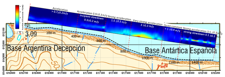
Figure 8 Distribution of the interpreted non-linear behaviour and short-term erosion trends (in m yr⁻¹) with the best fitted model (SL4) in the six recognised sectors in which the study area has been segmented.

By demonstrating the value of long-term, high-resolution, uncertainty-weighted regression modelling, our study provides an improved analytical baseline for understanding cliff dynamics under climate stressors. The sigmoidal models, in particular SL4, revealed erosion velocity spatial variability (0–400 m: $R=\mathrm{0.7}\pm \mathrm{0.17}\mathrm{m}{\mathrm{yr}}^{-\mathrm{1}}$ accelerating, 400–600 m: $R=\mathrm{0.9}-\mathrm{0.3}\pm \mathrm{0.25}\mathrm{m}{\mathrm{yr}}^{-\mathrm{1}}$ accelerating and incipient decreasing, 600–800 m: $R=\mathrm{1.5}\pm \mathrm{0.25}\mathrm{m}{\mathrm{yr}}^{-\mathrm{1}}$ accelerating, 800–1100 m: $R=\mathrm{3}\pm \mathrm{0.25}\mathrm{m}{\mathrm{yr}}^{-\mathrm{1}}$ accelerating, 1100–1200 m: $R=\mathrm{1}\pm \mathrm{0.35}\mathrm{m}{\mathrm{yr}}^{-\mathrm{1}}$ slightly slowing), and peaks as high as $\mathrm{3.5}\pm \mathrm{0.32}\mathrm{m}{\mathrm{yr}}^{-\mathrm{1}}$ (between 1200–1500 m), followed by marked deceleration – features missed by both linear and polynomial fits. The comparative diagnostic statistical analysis demonstrates that sigmoidal models outperform linear formulations in describing shoreline evolution, not only in terms of the standard error (RMSE) which remained consistently below 0.4 (with weighting), or goodness-of-fit (high R², mostly above 0.95 %) but also when accounting for model parsimony (AICc). These statistics outperformed those of linear and quadratic models across all zones, especially in the central 600–1100 m shoreline range. This supports their use as an appropriate representation of the observed non-linear behaviour. However, it is important to emphasise that this improved performance reflects a better empirical description of the data rather than a direct validation of underlying physical mechanisms.

It should be noted that the apparent post-2000 acceleration may be partially influenced by the higher temporal resolution of observations during this period, which can affect the stability of non-linear model fitting and the precise timing of inferred inflexion points. To assess the potential influence of temporal sampling density, a simple sensitivity test was performed by reducing the number of post-2000 observations to achieve a more homogeneous temporal distribution across the full time series (results from the time-homogenised dataset are provided as Supplement). The sigmoidal behaviour and general pattern of accelerated retreat were preserved under this reduced dataset, although the precise timing of the inflexion point showed minor variations. This proposes that the identified non-linear trend is not solely an artefact of increased sampling density in recent decades, but reflects a robust feature of the shoreline evolution.

The actual erosion rates observed in this study can be better understood when placed within a broader polar context. Arctic permafrost coasts are among the most rapidly eroding environments globally, with mean retreat rates typically ranging between ∼0.5 and 1.2 m yr⁻¹, and local maxima exceeding several metres per year in ice-rich bluffs, consistent with the combined effects of thermal degradation and wave action (e.g. Lantuit et al., 2012; Barnhart et al., 2014a; Gibbs and Richmond, 2017; Gibbs et al., 2019; Jones et al., 2020). In contrast, coastal erosion in the Antarctic Peninsula and South Shetland Islands remains comparatively less well quantified, possibly reflecting both lower marine energy conditions in many settings and the scarcity of long-term observational datasets Reported rates in Antarctic ice-free coastal sectors are typically lower, but highly variable, depending on local geomorphological and permafrost conditions and fitted linearly (Torrecillas et al., 2024).

Within this framework, the rates obtained for the study area in Port Foster can be considered moderate at the system scale, but locally significant. While much of the coastline exhibits relatively low to moderate retreat, specific sectors show markedly higher rates, reaching several metres per year, particularly in areas affected by concentrated hydrological flow and permafrost degradation. This highlights the importance of local controls and threshold behaviour, where spatial variability in ground-ice content, sediment properties, and moisture availability governs the response to external forcing. These findings support the interpretation that Antarctic periglacial coasts, although generally less energetic than their Arctic counterparts, can exhibit comparable short-term erosion magnitudes under favourable particular conditions. At the same time, the limited availability of comparable long-term datasets in Antarctica underscores the relevance of this study in contributing to a still emerging regional framework of coastal change.

The observed acceleration in cliff retreat after 2000, identified through the sigmoidal behaviour of the shoreline position time series, might be interpreted here as a threshold-type response of the periglacial coastal system to cumulative environmental forcing, rather than the result of a single external driver. The Antarctic Peninsula region is characterised by pronounced spatial and temporal climate variability, including alternating periods of warming and partial stabilisation (Turner et al., 2016; Oliva et al., 2017), which complicates direct attribution of geomorphic change to atmospheric trends alone. However, longer-term records indicate an overall warming tendency, punctuated by extreme events and recent heat anomalies (González-Herrero et al., 2022; Gorodetskaya et al., 2023; Roland et al., 2024), consistent with progressive perturbation of permafrost systems. In maritime Antarctic environments, permafrost is typically discontinuous, shallow, and highly heterogeneous, with strong sensitivity to local controls such as snow cover, lithology, and moisture availability (de Pablo et al., 2013, 2016; Hrbáček et al., 2017, 2023). Active layer thickness (ALT) exhibits marked spatial and temporal variability, with long-term deepening trends at some sites but significant interannual fluctuations linked to snow insulation and short-lived climatic extremes (Baptista et al., 2025). In coastal settings such as Deception Island, this variability is further amplified by hydrological complexity, the presence of porous volcanic substrates and geothermal anomalies, where changes in ground-ice content could directly influence geomechanical properties (Goyanes et al., 2014a; Ramos et al., 2017).

Within this framework, climate forcing does not act as a direct driver of erosion rates, but as a control on the thermal and hydrogeological state of the substrate, which in turn governs its mechanical response to marine forcing. The post-2000 inflection point is interpreted as the crossing of a system-specific stability threshold, whereby cumulative thermal and hydrological changes reduce the mechanical strength of ice-rich permafrost materials. The progressive loss of cohesion in the tephra–ice matrix, combined with increased water availability and sediment mobility, enhances slope instability and sediment supply to the coastal system. This preconditioning increases the sensitivity of the cliff to marine forcing, such that episodic events (e.g. storms, wave impact) can trigger disproportionately large retreat. Field observations in the South Shetland Islands support the occurrence of intensified geomorphic activity, including gully formation and mass wasting, during recent decades (Silva-Busso et al., 2013; de Pablo et al., 2016).

The geological characteristics of the cliff provide an important framework for interpreting the observed erosion dynamics. The study area is predominantly composed of poorly consolidated volcanic tephra, forming a relatively homogeneous lithological unit at the macroscopic scale. However, its mechanical behaviour is strongly modulated by the presence of ground ice and variable moisture conditions, resulting in a thermally sensitive composite material. In periglacial conditions, the strength of such materials depends not only on their granular properties but also on the ice content and its phase state. Consequently, spatial variations in permafrost distribution, active-layer thickness, and water saturation can produce significant heterogeneity in geomechanical properties along the bluff. This may explain why erosion rates could vary over short distances, despite limited lithological contrast.

Importantly, the marked spatial variability in permafrost conditions and the scarcity of long-term, integrated datasets mean that it is not possible to attribute the observed acceleration to a single determining factor, nor to define a uniform regional timeline for this post-2000 transition. Instead, the identified non-linear behaviour could be indicative of an emergent response to interacting thermal, hydrological, and marine processes, consistent with threshold dynamics reported in other permafrost-affected coastal systems. This transition from a quasi-stable state to an accelerated erosion regime is described. The pronounced spatial variability in cliff retreat observed along the study area may indicate the strong influence of localised controls. In particular, enhanced erosion near the river mouth suggests the importance of hydrological and thermal processes, where concentrated surface and subsurface flow can increase heat transfer into the ground and promote permafrost degradation. This leads to a reduction in the mechanical strength of ice-rich sediments, favouring localised slope instability and episodic mass wasting. Such behaviour highlights the role of internal preconditioning, whereby spatial differences in ground-ice content, active-layer thickness, and sediment properties generate heterogeneous responses to external forcing. In this context, marine processes act primarily as a triggering mechanism, while the spatial pattern of erosion is largely governed by variability in subsurface conditions. In addition, the proximity of the Argentine and Spanish research stations may introduce localised anthropogenic effects, including heat dissipation, modification of drainage, or surface disturbance. Although these influences cannot be quantified with the available data, they may contribute to small-scale variability and should be considered in future site-specific investigations.

This behaviour reinforces the interpretation of the system as a non-linear, threshold-controlled environment, in which relatively small changes in thermal, hydrological and subsurface conditions can lead to disproportionate geomorphological responses once critical weakening of the material has occurred. The observed non-linear and spatially heterogeneous erosion patterns can be understood as the result of interacting internal and external controls (Paredes et al., 2015), where progressive permafrost degradation conditions the mechanical response of the cliff, while marine forcing acts as a triggering mechanism modulating sediment removal.

A further aspect concerns the potential temporal relationship between climatic variability and retreat rates. Although the available dataset does not allow for a direct statistical correlation between temperature anomalies and shoreline change, the observed post-2000 acceleration broadly coincides with a period of increased climatic variability in the Antarctic Peninsula region, characterised by overall warming trends punctuated by short-term cooling episodes and extreme events. In permafrost-dominated coastal systems, such variability is expected to produce delayed and non-linear geomorphic responses, as ground thermal regimes integrate cumulative forcing over time. This implies that erosion rates may not respond synchronously to atmospheric temperature fluctuations, but rather reflect the progressive adjustment of subsurface thermal and hydrological conditions. Within this framework, the acceleration in retreat can be interpreted as the outcome of a time-lagged response to prior warming, potentially amplified by episodic extreme events. Establishing robust quantitative relationships between climatic drivers and coastal change, however, requires higher temporal resolution datasets and coupled monitoring of atmospheric, oceanic, and ground thermal conditions in Antarctic environments.

In conjunction with thermal preconditioning, marine forcing may influence modulating the spatial variability of cliff retreat. While the primary focus of this study is on the identification of non-linear temporal behaviour in cliff retreat, it is important to consider the role of marine forcing in controlling coastal erosion processes. In the study area, available evidence suggests that wave energy is generally low under mean conditions, but may increase significantly during episodic high-wind events, leading to enhanced sediment redistribution and localised cliff toe erosion. Although the study area is partially sheltered from the dominant regional wave climate in the semi-enclosed configuration of Port Foster, coastal processes remain relevant but operate in a modified regime. Under typical conditions, wave energy is relatively low, limiting the role of continuous marine abrasion. However, episodic high-wind events can locally enhance wave activity and contribute to sediment redistribution and cliff toe erosion. Numerical simulations of wind-driven waves (Caballero-Martínez et al., 2025) indicate generally low wave energy (heights<0.3 m) with dominant W–WSW directions, promoting westward alongshore transport and localised accretion in the western sector, while central and eastern areas exhibit mixed erosion–accretion patterns. The agreement between modelled transport and shoreline evolution suggests that alongshore sediment gradients alone cannot explain the observed retreat. Under extreme wind conditions ($>\mathrm{15}\mathrm{m}{\mathrm{s}}^{-\mathrm{1}}$), sediment transport increases markedly, enhancing redistribution over short timescales. However, the spatial mismatch between transport maxima and retreat rates indicates that alongshore processes are not the primary driver of erosion. Instead, cross-shore energy transfer and wave action at the cliff toe likely play a more significant role. Accordingly, marine forcing acts as a triggering mechanism: when permafrost materials are thermally weakened, even low-energy wave activity can promote undercutting and removal of sediment. In addition, regional variability in sea-ice extent and storminess can influence coastal exposure by modifying wave fetch and the frequency of high-energy events. This supports a coupled interpretation in which episodic storm events and variability in coastal exposure modulate erosion in a preconditioned periglacial system. However, marine processes alone do not fully explain the observed spatial and temporal patterns of erosion. Instead, their effect must be understood in conjunction with the evolving mechanical properties of the cliff material. In permafrost-affected coasts such as Deception Island, progressive thermal degradation leads to a reduction in cohesion and shear strength within the ice-rich tephra, increasing the susceptibility of the cliff to external forcing.

In this context, cliff retreat could be best interpreted as a coastal–periglacial process, in which internal degradation mechanisms – such as permafrost thaw, active-layer deepening, and hydrogeologically driven weakening – control the mechanical state of the material, while marine forcing acts as a secondary but necessary triggering mechanism. Marine dynamics act primarily as a triggering mechanism, facilitating the removal of already weakened material rather than acting as the dominant driver of erosion. This coupling may explain how significant erosion can occur even in relatively sheltered environments, where the system remains sensitive to moderate external perturbations once internal weakening has taken place. Our interpretation highlights the importance of considering both internal (thermal and hydrological) and external (marine) controls, whose interaction can produce non-linear and spatially heterogeneous erosion responses. Future work should aim to disentangle these contributions through integrated datasets combining shoreline evolution, oceanographic forcing, and ground thermal monitoring.

Given the observed acceleration and deceleration in coastal erosion – especially evident between 2000 and 2023 year – this study underscores the need for dynamic models in coastal geomorphology, capable of capturing time-varying responses to environmental forcings, heterogeneous distribution of permafrost and other subsurface complexities, and real scale capabilities (Omonigbehin et al., 2025). As satellite archives expand and UAV deployments become more feasible in polar regions, the field is poised to transition from static assessments of coastal change to dynamic, process-based modelling. The future of Antarctic coastal research lies in combining such models with real-time environmental monitoring and thermal imaging to link atmospheric anomalies, permafrost degradation, and morphological change.

Despite these contributions, the study has several limitations. First, the reliance on manual digitisation, while necessary due to low image contrast in some historical datasets, introduces subjectivity. Future work should explore semi-automated edge-detection algorithms (Swirad and Young, 2021, 2022; Lu et al., 2024) to reduce operator bias. Second, while our temporal resolution is high for an Antarctic site, annual or seasonal imagery remains unavailable, limiting insights into intra-annual variability or responses to extreme events. Efforts should be made to integrate UAV photogrammetry and satellite altimetry in upcoming campaigns to refine temporal granularity. Additionally, the study is geographically restricted to a 1.5 km segment. While representative, caution is warranted when extrapolating results to the broader South Shetlands or Antarctic Peninsula. Comparative studies across multiple Antarctic sites – and against Arctic analogues – could illuminate regional controls on erosion heterogeneity. Finally, more detailed ground temperature and permafrost stratigraphy data would allow coupling of physical drivers with morphological responses, moving from correlative to process-based models.

Beyond scientific advancement, the implications of this work extend to environmental management and policy. With several research bases situated within 200 m of retreating cliffs, a clear need arises for integrated erosion monitoring frameworks. Our work offers authorities a decision-support tool to identify risk-prone sectors and develop tailored protection strategies. The incorporation of spatially explicit uncertainty weighting is particularly valuable for producing credible early-warning signals in logistical planning for seasonal base activities. Therefore, this study advances the understanding of Antarctic periglacial coastal erosion by: (i) demonstrating the failure of linear regression to adequately represent long-term shoreline evolution, (ii) demonstrating that sigmoidal models better capture the observed non-linear dynamics of shoreline retreat than linear formulations, based on comparative statistical performance, within the limits of the available dataset, (iii) emphasising the importance of uncertainty-informed weighting in statistical coastal analyses, (iv) highlighting strong spatial heterogeneity in erosion rates linked to local geomorphology and infrastructure, and (v) offering a transferable methodological framework for high-latitude cliff monitoring using legacy imagery.

The identified non-linear behaviour of cliff retreat has important implications for infrastructure located in coastal sectors of Deception Island, particularly the nearby scientific bases. Although the present study does not aim to perform a formal risk assessment, the observed acceleration in erosion rates suggests that shoreline stability may decrease over relatively short timescales once critical thresholds are exceeded. In this context, the transition from a quasi-stable state to an accelerated retreat regime implies that coastal change may not proceed gradually, but rather through episodic and potentially rapid adjustments. This behaviour introduces significant uncertainty in the long-term stability of coastal landforms, especially in areas where infrastructure is located close to actively retreating cliffs.

Furthermore, the coupling between permafrost degradation and marine forcing suggests that future changes in climatic and oceanographic conditions – such as increased ground temperatures, reduced sea-ice extent, or more frequent high-energy events – may enhance the susceptibility of coastal sectors to erosion. As a result, even in the absence of continuous high-energy forcing, the system may remain sensitive to relatively moderate perturbations once mechanical weakening has occurred. These findings highlight the need for continued monitoring of shoreline evolution and permafrost conditions in the vicinity of scientific bases, as well as the incorporation of non-linear coastal behaviour into future hazard and risk assessments. In particular, the use of high-resolution temporal datasets and integrated process-based approaches will be essential to improve the predictability of coastal change in Antarctic periglacial environments.

7 Conclusions

This study contributes both methodologically and conceptually by linking non-linear statistical modelling with a process-based interpretation of coastal–periglacial dynamics. We address here the pressing need to refine methodologies for understanding and predicting coastal erosion in periglacial environments, focusing on the volcanic bluffs of Port Foster, Deception Island. Through a comprehensive analysis of a 66 year time series derived from historical aerial photography and satellite imagery, this research demonstrates that coastal retreat in Antarctic settings is inherently non-linear. Periods of accelerated erosion, particularly after ∼2000, alternate with intervals of relative stability. Traditional linear models proved inadequate in capturing these dynamics, often underestimating erosion rates and failing to represent episodic behaviour observed in the field.

In contrast, the application of sigmoidal logistic models yielded a significantly improved characterisation of threshold-like transitions in cliff retreat. These models enabled the identification of inflection points in erosion rates and provided a more realistic empirical representation of the observed geomorphological behaviour. The integration of uncertainty-weighted regression further strengthened model robustness, mitigating biases associated with variable data quality across the historical image archive. This approach sets a precedent for future analyses in data-scarce polar environments, where heterogeneity in imagery is common.

Methodologically, the study underscores the value of combining structure-from-motion photogrammetry, orthorectification, and SCA-TBM analysis within a GIS framework. While positional uncertainties inherent in older datasets introduce some limitations, the consistent application of ground control points and robust statistical weighting ensures that detected shoreline changes reflect genuine geomorphological trends. The SCA-TBM approach, coupled with uncertainty analysis, offers a replicable and scalable strategy for long-term coastal monitoring.

From a process-based perspective, the observed erosion patterns are best interpreted within a coupled coastal–periglacial system, in which internal factors – such as permafrost degradation, active-layer dynamics, and hydrological processes – control the mechanical state of the cliff material, while marine forcing acts primarily as a secondary triggering mechanism. In this context, the post-2000 acceleration is interpreted as the expression of a threshold response associated with progressive weakening of ice-rich sediments, rather than as the direct result of a single external driver. The study also highlights pronounced spatial heterogeneity in erosion rates, consistent with localised variations in permafrost conditions, geomorphology, and hydrological concentration, with possible additional influence from nearby infrastructure.

Despite these trends, erosion rates in Port Foster remain lower than those typically reported in Arctic permafrost coasts, reflecting differences in coastal energy regimes and environmental forcing. Practically, the results underscore the need to integrate non-linear models into coastal risk assessments and infrastructure planning in Antarctica. The proximity of scientific installations to actively retreating cliffs amplifies the urgency for mitigation strategies grounded in realistic representations of coastal dynamics. The demonstrated utility of non-linear regression models suggests they should be incorporated into future coastal vulnerability assessments, both in the Antarctic and other permafrost-affected regions.

Looking ahead, future research should expand spatial and temporal datasets, integrate extreme event analysis, and develop coupled observational frameworks combining shoreline evolution, oceanographic forcing, and ground thermal monitoring. Such approaches will be essential to improve process understanding and predictive capability in rapidly changing periglacial Antarctic coastal environments.