Brief communication: Inferring Glacier Equilibrium Line Altitudes in the Europe Alps with FROST

The current pace of glacier retreat in the European Alps is unprecedented in the observational record and has significant implications for water resources and downstream ecosystems. Quantifying the future evolution of these systems requires physically based glacier models that are calibrated against observational data. Using the open-source Framework for assimilating Remote-sensing Observations for Surface mass balance Tuning (FROST), we infer mean Equilibrium Line Altitudes (ELAs) and other surface Mass Balance (SMB) parameters for 409 Alpine glaciers for the time period 2000–2019 using an Ensemble Kalman Filter. The method combines an elevation-dependent SMB model with ice dynamics from the Instructed Glacier Model (IGM). Validation against ELA estimates from in-situ measurements and end-of-summer snowline data shows good agreement, with Pearson correlation coefficients of r=0.74 and r=0.64, respectively. These results demonstrate that FROST enables satellite-based calibration of SMB parameters at regional scale. This study serves as a first step toward a more general framework for transient data assimilation in glacier modeling.

1 Introduction

Mountain glaciers are losing mass worldwide in response to anthropogenic climate change (Zemp et al., 2025) and are currently among the largest contributors to sea-level rise, comparable to the combined meltwater from Greenland and Antarctica (Slater et al., 2021). In the European Alps, roughly 4000 glaciers were cataloged around the year 2000 (RGI Consortium, 2023), but most are projected to disappear by the end of the century due to climate change (Zekollari et al., 2025) or have already disappeared. At present, glaciers in the European Alps play important roles in local hydrology (Koboltschnig and Schöner, 2011) and hydroelectric power generation (Schaefli et al., 2019). In Switzerland alone, around 200 000 people live in areas directly influenced by glacier meltwater, glacial lakes, or periglacial processes (Huss et al., 2017). Their retreat has already shifted seasonal runoff patterns (Huss and Hock, 2018), increased the risk of landslides (Haeberli et al., 2017), and led to the formation of new proglacial lakes, underscoring the urgency to better understand their evolution and associated risks in this densely populated region.

Accurate modeling of glacier evolution requires a realistic representation of both the Surface Mass Balance (SMB) and the ice dynamics. The SMB quantifies all processes of surface accumulation and melt. Existing SMB models range from simple temperature-index approaches to physically based energy balance models (Hock et al., 2019). At the scale of individual glaciers or catchments, a wider range of calibration data is typically available, including in-situ observations and weather stations. In contrast, at regional to global scales, SMB model calibration is more weakly constrained and has often relied on matching scalar geodetic mass balance estimates derived from datasets such as Hugonnet et al. (2021a), for example in OGGM v1.6 (Maussion et al., 2023), PyGEM (Rounce et al., 2023), or more recently on snowline altitude (Cremona et al., 2025). However, these approaches strongly reduce the spatial information contained in modern remote-sensing products, such as elevation change or velocity fields (Hugonnet et al., 2021a; Sommer et al., 2020). Efficient methods are therefore needed to assimilate such spatially distributed datasets directly into the calibration process.

The representation of ice dynamics is equally essential for glacier modeling. Flow-line models remain widely used due to their computational efficiency and ability to reduce glacier geometry to its key dimensions: length, thickness, and surface elevation along a central flow line (Maussion et al., 2019; Rounce et al., 2023). In an recently published study of Schmitt et al. (2026) they add inversion of thickness along the flowline to OGGM based surface elevation, volume estimate and elevation change. This approach moves towards data assimilation, where multiple observational constraints are combined to infer consistent glacier states. With the recent development of the IGM (Jouvet and Cordonnier, 2023), it has become feasible to simulate three-dimensional glacier flow at a reasonable computational cost. IGM also enables the inversion for ice thickness and an additional sliding coefficient field that represents unresolved processes influencing surface velocity that are not explained by ice thickness or bed slope alone. While satellite-based velocity products are increasingly available (Friedl et al., 2021; Millan et al., 2022), they are rarely used for model calibration in large-scale glacier modeling frameworks.

Ensemble-based data assimilation methods such as the Ensemble Kalman Filter (EnKF) (Evensen, 1994) have gained traction in glaciology for parameter and state estimation. The EnKF offers a derivative-free alternative to adjoint-based methods (Higdon et al., 2012; Iglesias et al., 2013), which, in contrast, require gradient computations and full access to the model internals. Applications include ensemble transform Kalman filter-based parameter estimation (Bonan et al., 2014) and assimilation of surface observations in ice sheet models (Gillet-Chaulet, 2020). Variational approaches, such as adjoint methods (Goldberg and Heimbach, 2013), remain powerful but computationally demanding. Recent work by Knudsen et al. (2024) and Herrmann et al. (2025) demonstrated the potential of EnKF for calibrating SMB parameters in a synthetic glacier setting.

Building on the FROST introduced by Herrmann et al. (2025), we calibrate SMB model parameters against elevation-change observations from 2000–2019 for the 409 glaciers in the European Alps that exceeded 1 km² in RGI7. This size threshold is chosen to ensure that glacier areas are sufficiently large to resolve spatial patterns in elevation change and SMB relative to observational noise. The framework combines the three-dimensional glacier evolution model IGM with an EnKF to iteratively calibrate elevation-dependent SMB parameters. This approach enables the calibration of glacier-specific ELAs and mass-balance gradients, where the ELA represents the altitude separating accumulation and ablation and the gradients describe how these mass balance changes with elevation. We focus on 20-year spatial patterns of accumulation and ablation, because elevation-change observations over a longer time period provide more robust constraints compared to shorter periods (e.g., 5-year). The inferred ELAs are validated against independent EoS SLA derived from remote sensing (Sommer et al., 2026a) and in-situ SMB measurements from GLAMOS (2023) and WGMS (2024), demonstrating that FROST enables satellite-based calibration of SMB parameters at regional scale. This study provides a simplified test case for transient data assimilation, where observations are assimilated at their time of acquisition. This enables a more accurate simulation of glacier systems and leverages the growing availability of remote sensing data. The framework is readily extendable in this direction, as the underlying EnKF is inherently designed for sequential data assimilation. By reducing the complexity of the problem to one observation period, we provide a first step toward identifying challenges on the way to fully transient data assimilation in glacier modeling.

2 Data and Method

The FROST v1.0.0 pipeline (Herrmann et al., 2025) integrates the IGM v3.0.0 (Jouvet and Cordonnier, 2023) with the EnKF (Evensen, 1994) to estimate glacier-specific SMB parameters. The SMB model used here is an elevation-dependent piecewise-linear function and does not take climate variables as input (Eq. 1).

$$\begin{array}{}\text{(1)}& \mathrm{SMB}\left(z\right)=\left\{\begin{array}{ll}{\mathit{\beta }}_{\mathrm{acc}}\cdot (z-z_{\mathrm{ELA}})& \text{if }z>z_{\mathrm{ELA}},\\ {\mathit{\beta }}_{\mathrm{abl}}\cdot (z-z_{\mathrm{ELA}})& \text{otherwise}.\end{array}\right.\end{array}$$

where z denotes the elevation of the glacier surface, z_ELA the ELA, β_acc and β_abl the accumulation and ablation gradients, respectively. The EnKF is used to iteratively update SMB parameters by minimizing the misfit between modeled and observed elevation change. The prior distributions of the SMB parameters are derived from measurements of eleven glaciers in the GLAMOS dataset covering the period 2000–2019. We assume Gaussian priors, with standard deviations set to three times the corresponding GLAMOS standard deviations. The resulting priors are: $z_{\mathrm{ELA}}=\mathrm{3144}\pm \mathrm{498}$ m, ${\mathit{\beta }}_{\mathrm{abl}}=\mathrm{7.55}\pm \mathrm{8.04}$  m a⁻¹ km⁻¹, and ${\mathit{\beta }}_{\mathrm{acc}}=\mathrm{3.09}\pm \mathrm{3.39}$ m a⁻¹ km⁻¹. It is worth noting that IGM assumes a constant ice density of 910 kg m⁻³. A detailed description of the FROST is provided in Herrmann et al. (2025).

The framework utilizes OGGM-shop to download, align, and pre-process surface elevation (Crippen et al., 2016), surface velocity (Millan et al., 2022), thickness measurements (Welty et al., 2020), and glacier outlines from the RGI7 (RGI Consortium, 2023). The IGM v3.0.0 inversion for ice thickness and basal sliding includes several optimization parameters, which were manually tuned based on examples provided in the IGM repository. The goal was to balance the tendency to overestimate thickness for small glaciers against underestimation for large glaciers. A first qualitative assessment was based on visual inspection (e.g. Fig. S4). Since the inversion of 409 glaciers is computationally costly, we tested a small number of different parameter sets and selected the one that provided the best agreement with observed surface velocities. This evaluation was based on summary statistics, including the mean, quantiles, and extremes of the velocity distributions.

As a calibration target for the EnKF, we use the elevation-change product from Hugonnet et al. (2021a), which provides globally gridded elevation change rates between 2000 and 2019 at 100 m resolution. These rates are added to the NASADEM elevation data to reconstruct the 2019 surface topography, with the associated uncertainties in elevation change propagated into the 2019 elevation uncertainty. The chosen calibration parameters, whose roles are described in more detail in Herrmann et al. (2025), are an ensemble size of 36, an elevation bin size of 50 m, and six iteration steps. The exact code is available at https://github.com/FAU-glacier-systems/FROST/tree/main/experiments/central_europe_submit, last access: 27 May 2026.

For validation, we compare the calibrated SMB parameters with independent glaciological measurements from GLAMOS (2023) and WGMS (2024). Multi-year mean ELA values and SMB gradients are derived from elevation-binned mass balance data by computing the 20-year mean for each elevation bin and fitting a two-segment piecewise-linear function separated at the ELA (see Fig. S10). For a meaningful accumulation gradient, we require a minimum of three elevation bands with positive mass balance. To ensure representative estimates of the period, we only include glaciers with more than ten years of ELA observations. Based on our sampling analysis, this corresponds to an average uncertainty of approximately 25 m relative to the 20-year mean, with occasional outliers reaching up to 100 m (see Fig. S9).

To further evaluate the inferred ELAs, we compare them to End-of-Summer Snow Line Altitude (EoS SLA) derived from Landsat and Sentinel-2 imagery (Sommer et al., 2026a). The distinction between areas of bare glacier ice and snow cover is automatically estimated by intensity thresholds from infrared reflectance histograms based on Otsu's method (Otsu, 1979). Thereby, the glacier area covered by snow is identified due to the relatively high near- (NIR) and shortwave-infrared (SWIR) reflectance of snow compared to bare ice or debris (Hall et al., 1987). The date-specific snow line altitude is then derived by masking the surface elevations of the NASADEM with the pixels classified as snow. For each glacier and year, the EoS SLA is defined as the highest transient snowline observed during the late ablation season (15 July–30 September). Estimates based on fewer than three suitable satellite scenes were subjected to outlier detection, as a minimum of three scenes is required to ensure sufficient temporal coverage of the late ablation period. For glaciers with at least ten valid years, values deviating by more than ±2 standard deviations from the glacier-specific mean were removed; for glaciers with fewer than ten valid years, an additional physical threshold excluded EoS SLAs differing by more than 400 m from the mean glacier elevation (RGI v7). The mean EoS SLA for 2000–2019 was then computed from all non-flagged years and serves as an independent benchmark for evaluating the calibrated ELA values. For more details we refer to Sommer et al. (2026a). The comparison is assessed using the Pearson correlation coefficient and Mean Absolute Error (MAE).

3 Results

We applied the method described in Sect. 2 to the glaciers in the European Alps and calibrated glacier specific ELA for 409 glaciers. Here, we summarize regional patterns, validation against dataset from Glacier Monitoring Switzerland (GLAMOS) and World Glacier Monitoring System (WGMS), and compare with EoS SLA extracted from optical imagery.

3.1 Regional equilibrium line altitude distribution

Our calibration results yield an ELA range from 2540 to 3540 m a.s.l. for the period 2000–2019, with a mean of 3158 m a.s.l. and a standard deviation of 157 m. The spatial distribution of modeled ELAs reflects the main climatic gradients across the Alps: lower values occur along the northern and western flanks, while higher values dominate in the higher inner Alps (Fig. 1). The equivalent maps for the calibrated gradients are provided in the supplements (Figs. S2 and S3). While ELAs correlate with mean glacier elevation, no other systematic relationship with glacier size or aspect emerges at the scale of the entire Alps (see Fig. S1), although in subregions the observed spread is likely influenced by hypsometry and exposure (Rettig et al., 2026). Local deviations can further arise from shading, debris cover, and other surface or topographic effects, which were not investigated in this study.

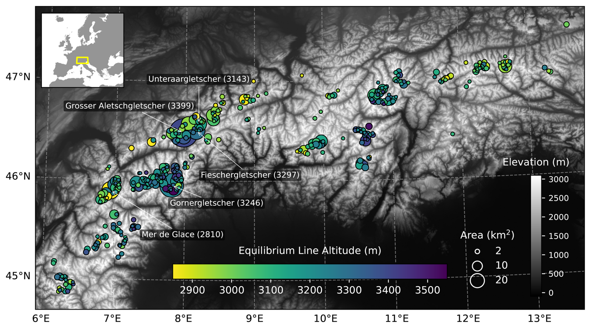
Figure 1 Mean ELA of glaciers in the European Alps for the period 2000–2019, calibrated using FROST. Circle color indicates the ELA, and circle size is proportional to glacier area. Five large glaciers are labeled with their names and the calibrated ELA in parentheses. Background topography © EuroGeographics.

3.2 Validation with end-of-summer snow line altitude

The modeled and observed mean elevation change of the individual glaciers show a strong agreement (Fig. 2a), with a correlation of r=0.88 and a MAE of 0.13 m yr⁻¹. Also the ELA correlation with EoS SLA, as indicated by a Pearson correlation of 0.64. The MAE of 180 m is partly driven by a bias of +135 m, which can be attributed to a systematic underestimation of the EoS SLA, since the underlying imagery do not necessarily capture the day of maximum snowline retreat. After bias correction, the MAE decreases to 126 m (MAE^*) (Fig. 2b).

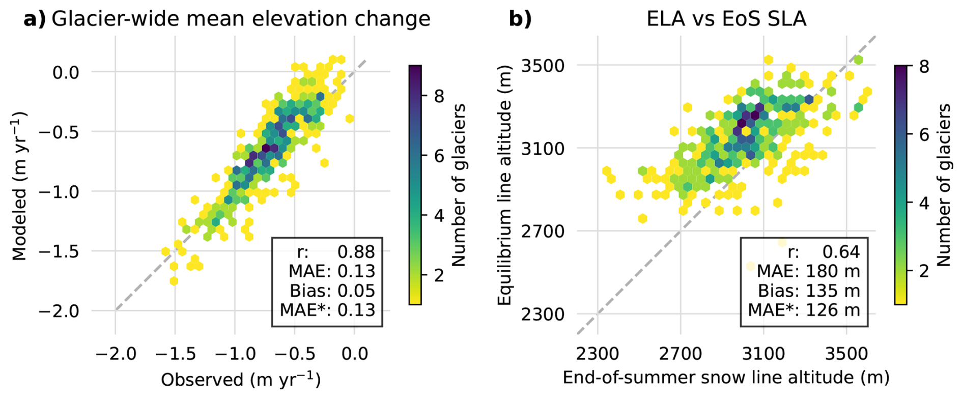
Figure 2 Comparison with observed glacier-wide elevation change (Hugonnet et al., 2021a) and End-of-Summer Snowline Altitudes (EoS SLAs). Panel (a) shows modeled and observed elevation change, and panel (b) shows calibrated ELA and EoS SLA. Both panels use hexagon density plots, where color indicates the number of glaciers per bin. The total sample number is 409. Pearson correlation coefficients (r), MAE, and bias-corrected MAE (MAE^*) are reported in each panel.

3.3 Validation against glaciological observations

The modeled and observed ELAs show consistent agreement across a range of glaciers, with r=0.74 and a MAE of 106 m. The only notable outlier is Grosser Aletschgletscher, where the calibrated ELA (3399 m a.s.l.) substantially exceeds the observed value (3034 m a.s.l.). The mass balance gradients show considerably weaker agreement: the ablation gradient yields r=0.12 and a MAE of 4.07 m w.e. yr⁻¹ km⁻¹, and the accumulation gradient r=0.22 and a MAE of 1.56 m w.e. yr⁻¹ km⁻¹. Modeled and observed mean elevation change are in good agreement (r=0.94, MAE = 0.12 m w.e. yr⁻¹), as expected since it is used as the calibration target. The Hugonnet et al. (2021a) elevation change dataset and the glaciological mass balance observations show a strong correlation (r=0.74), supporting the use of the former as a calibration target and the latter as an independent evaluation dataset. The ice-dynamic parameters show broad agreement with observations that are used in the ice-dynamic calibration, with r=0.77 for ice thickness and r=0.61 for surface velocity. Grosser Aletschgletscher is an outlier in both thickness and velocity, and Plaine Morte is an additional outlier in the thickness comparison. These results are summarized in Fig. 3. The velocity comparison between modeled and observed values for all glaciers, along with additional metrics including mean, quantiles, and extremes, is shown in Fig. S4.

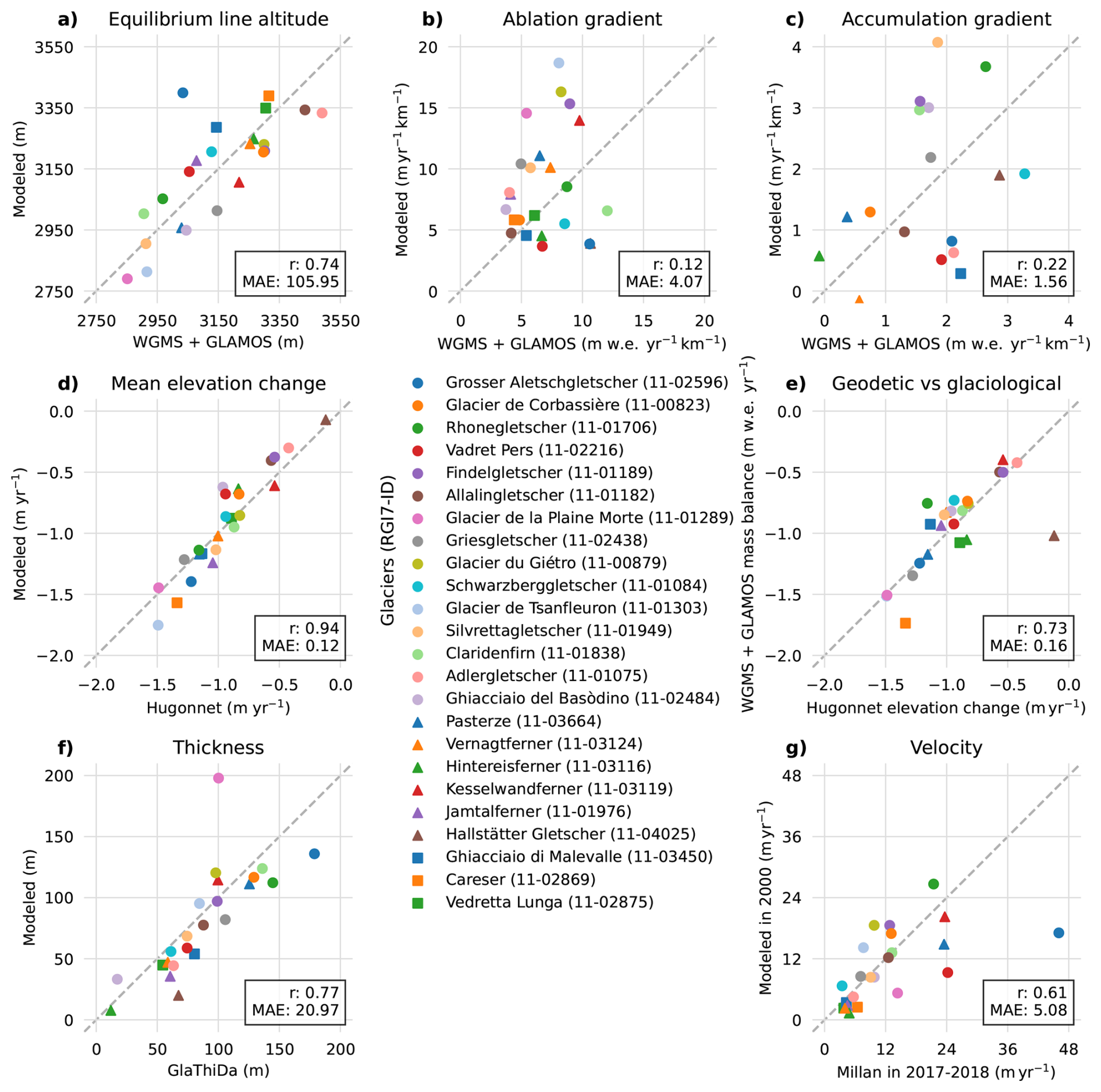
Figure 3 Validation against glaciological observations. Sub-panels show (a) ELA, (b) ablation gradient, (c) accumulation gradient, (d) mean elevation change used as EnKF target, (e) comparison of calibration target and evaluation data, (f) ice thickness, and (g) surface velocity. Pearson correlation coefficients and MAE are reported in each panel. Circles indicate glaciers in Switzerland, triangles in Austria, and squares in Italy.

4 Discussion

The results demonstrate that FROST enables a regional, observation-constrained calibration of SMB parameters and ELAs across the European Alps. To our knowledge, it is also the first regional calibration framework that explicitly incorporates the spatial information contained in elevation change observations. At the same time, the results highlight several limitations related to inversion settings, input data quality, and model assumptions. In the following, we discuss the main sources of inaccuracies and their impact on the calibrated parameters, and place the simplified experimental design of this study in the context of future developments toward fully transient data assimilation.

4.1 Uniform inversion settings

Achieving consistency between observed and modeled glacier velocity and thickness typically requires glacier-specific tuning of the IGM inversion parameters. Applying a single parameter set to all 409 glaciers inevitably stretches the inversion's capabilities, as no systematic procedure for automated tuning currently exists and manual adjustment for each glacier is not feasible. After extensive testing, we adopted a compromise parameter set for IGM v3.0.0, balancing the tendency to overestimate thickness in small glaciers against underestimation in large ones. A visual indicator for the regional agreement with velocity observation were Fig. S4. Grosser Aletschgletscher is particularly affected: at 81 km² it is by far the largest glacier in the dataset, with the second largest, Pasterze, covering 18.5 km². The current inversion settings result in an underestimated ice thickness and surface velocity for Aletschgletscher (Fig. S5), and the consequently reduced ice flux is compensated by a lower ablation gradient in the calibration. An adapted inversion parameter set would yield more realistic ice-dynamic parameters and, in turn, more physically consistent SMB calibration. However, to maintain a broadly applicable workflow, we retain a uniform parameter set. Future versions of IGM are expected to be less sensitive to parameter settings and, in general, more robust in reproducing the observed velocity field and inferring realistic thickness fields. A recently published study by Frank et al. (2026) also provides an alternative IGM-based thickness inversion approach, offering a promising initialization of the ensemble simulations.

4.2 Inaccuracies in the input datasets

Observation errors can propagate through the calibration. Elevation-change products such as Hugonnet et al. (2021a) rely on temporal aggregation and may exhibit local biases, particularly in accumulation areas with low surface contrast and steep slopes, where small horizontal errors can translate into large vertical offsets. We also observed unrealistically high velocity patches in the surface velocity fields from Millan et al. (2022) for several glaciers, including Plaine Morte (Fig. S6) and Glacier du Giétro (Fig. S7). These processing artifacts, in combination with uniform inversion settings, lead to unrealistically high ice fluxes towards the glacier tongue. This increased flux is compensated by higher ablation rates, which drives the calibrated ablation gradient to unrealistically large values. This mechanism likely contributes to the weak agreement in the ablation gradient (r=0.12, MAE = 4.07 m w.e. yr⁻¹ km⁻¹) reported above, with Plaine Morte and Glacier du Giétro representing extreme cases. These two glaciers also show unrealistic wave patterns in the glacier thickness, likely caused by inversion instabilities triggered by the velocity artifacts. Promising alternative for the velocity observations is the regional product of Rabatel et al. (2023) and the global velocity products of Friedl et al. (2021) and Gardner et al. (2025).

4.3 Assumptions of the SMB Model

The elevation-dependent SMB model neglects horizontal variability. This reduction to elevation is a common assumption in regional and global-scale glacier modeling. Although SMB and elevation change are primarily governed by elevation, lateral differences are not represented and can be significant, particularly in branching glaciers where flow and mass balance vary within the same elevation band due to azimuth, shading and small-scale precipitation variability. The piecewise linear parameterization of the mass balance profile is a reasonable first-order approximation, but does not fully capture the nonlinear altitudinal variability observed in glaciological measurements (see Fig. S10). These simplifications may contribute to the weak agreement in the ablation gradient. The accumulation gradient is additionally poorly constrained, as most glaciers in the European Alps have lost much of their accumulation area over the period 2000–2019, leaving few observations to anchor the gradient. However, since the accumulation gradient has a relatively minor influence on the overall mass balance compared to the ablation gradient and ELA, this limitation is of secondary concern.

4.4 Simplified temporal representation

The current study does not implement a fully transient data assimilation framework, but instead relies on a simplified setup using a single observation period (2000–2019). This implies that temporal inconsistencies between input datasets are not explicitly accounted for. In particular, the velocity product and RGI outlines may represent different periods, and potential glacier slowdown in the 21st century is not captured. Similarly, ice thickness observations are assumed to represent the glacier state in 2000, although they originate from years around 2000. These limitations may affect the consistency of inferred parameters and initial conditions. Extending the framework toward a fully transient data assimilation scheme that integrates time resolved observations represents an important direction for future work.

4.5 Sequential vs variational data assimilation

For fully transient data assimilation, it is also worth considering a 4DVar approach as explored by Schmitt et al. (2026) in a synthetic OGGM setup. In contrast to ensemble Kalman filter methods, 4DVar assimilates all observations within a single optimization window by minimizing a cost function over the full time period. This requires a differentiable model but yields a trajectory that is simultaneously constrained by all observations. The ensemble Kalman filter instead updates the model state sequentially in time and propagates uncertainty through an ensemble, which is more broadly applicable without requiring model adjustments but may introduce temporal smoothing or lag in the assimilation. Both approaches offer complementary strengths: 4DVar is particularly well suited when a differentiable model is available and a trajectory over a time window is required, whereas the ensemble Kalman filter is advantageous for high frequency observations and complex, non differentiable models, where the main interest is the final state of the system, for example for future projections.

4.6 Evaluation datasets

Validation against EoS SLA-based proxies and glaciological mass balance observations may show deviations that do not necessarily indicate calibration errors, but rather reflect that these products represent related, yet not identical, quantities. EoS SLA data are spatially aggregated and sensitive to threshold definitions, while mass balance data from GLAMOS and WGMS rely on interpolation between sparse stake measurements and may not capture localized variability. Sommer et al. (2026a) compare EoS SLA with ELA values reported by WGMS and reveal similar discrepancies to those found in this study, with estimated EoS SLA values occasionally lying below the reported ELA. One possible explanation is the absence of cloud-free observations capturing the highest snowline altitude at the end of the ablation season. In addition, firn areas may be classified as snow because of their similar reflectance properties, which can lead to underestimated snowline elevations when glacier ice is fully exposed. For glaciers with limited temporal coverage (e.g., only 10 ELA observations within the study period, such as Glacier de la Plaine Morte and Glacier de Tsanfleuron), the sampling uncertainty can reach up to 100 m, as the maximum seasonal retreat of the snow cover is likely not captured. A finer temporal resolution of the SMB model would allow direct comparison with point measurements. In contrast, our evaluation is based on aggregated and processed glaciological data.

5 Conclusion

The presented framework provides a regional calibration of SMB parameters for the period 2000–2019, including estimates of ELAs for all glaciers larger than 1 km² in the European Alps. Overall, the analysis demonstrates that the FROST reproduces SMB parameters and large-scale ELA patterns across the Alps, with good agreement with independent observations from GLAMOS and WGMS, and consistent relationships with EoS SLA. At the same time, the results highlight limitations. The framework remains sensitive to data quality and the initialization of ice dynamics, with inaccuracies in the input datasets and thickness inversion propagating into the calibrated parameters. Future versions of IGM are expected to reduce these effects and improve SMB parameter estimates.

The Python-based, open-source framework integrates IGM within an EnKF and offers strong potential for combining multiple remote sensing datasets. Here, we restrict the assimilation to a single observation period, providing a simplified test case. However, the EnKF naturally enables sequential assimilation and the incorporation of observations at their time of acquisition. Extending the framework toward transient data assimilation, including repeated elevation-change observations, snowline data, or surface velocities, is a logical next step. With these advances, FROST can enable more consistent and robust, observation-driven calibration of glacier models for regional monitoring and projection.