Mapping daily snow depth with machine learning and airborne lidar across two contrasting snowpacks

Daily, basin-scale snow depth maps are needed for forecasting and operations, yet airborne lidar typically provides only episodic snapshots. We present a portable relative-depth machine-learning framework that converts a small number of lidar acquisitions plus a single daily driver time series (in-situ station or ERA5-Land) into temporally coherent, per-pixel daily snow depth maps. A random forest model is trained on lidar–driver differences where lidar supplies the spatial pattern of departures and the driver supplies temporal evolution; learning is constrained to observed conditions using a valid-pixel mask and synthetic zero-depth maps at season start and end. We evaluate the approach in two contrasting regimes – Mores Creek, Idaho, and Hubbard Brook, New Hampshire – using multi-year lidar records. Across both basins, performance is fit for purpose (R² 0.89–0.90; RMSE 8–28 cm; MAE 5–19 cm; near-zero bias). Mores Creek, a larger heterogeneous western basin benefits more from adding lidar-informed residual maps, than Hubbard Brook, a smaller transitional eastern basins, where the primary value is correcting local departures from the mean and refining melt timing. Spatial diagnostics and Shapley values show that residuals are organized by landscape controls including elevation, aspect/northness, microtopography, slope, and a redistribution proxy. Lidar-cadence experiments indicate diminishing returns after a few acquisitions: roughly five flights in early season, four in mid-winter, and five in late season recover most skill at Mores Creek, while Hubbard Brook shows a similar pattern with about three flights in early-mid winter and five in mid-late winter, but with greater variability in model skill. The timing of lidar acquisitions also influences model transferability. Models trained on mid-season data generalize well to both early and late season conditions, whereas models trained on late-season data perform poorest when applied to early season dates. ERA5-driven runs closely track in-situ driven results, indicating the feasibility of using reanalysis datasets where stations are absent. The method is intentionally interpolative and should be applied within its area of applicability, but it offers a practical route from episodic lidar snow surveys to meter-scale, daily, basin-scale products and actionable guidance on survey timing and frequency.

1 Introduction

Seasonal snow cover provides valuable water for billions of people across the Northern Hemisphere. In the American West, snowmelt supplies roughly 53 % of annual runoff (Li et al., 2017), and both western and eastern snowpacks are projected to decline under future climate scenarios, with implications for water security, wildfire risk, soil freeze-thaw dynamics, and cold water habitats (Callaghan et al., 2011; Diffenbaugh et al., 2015; Ford et al., 2021; IPCC, 2023).These natural, social, and economic stakes underscore the importance of monitoring snow depth distribution and its seasonal evolution to improve water forecasting, guide resource allocation, and anticipate ecologic and hydrologic impacts. While in-situ networks such as snow courses and automated stations (e.g., SNOTEL) provide accurate point-scale snow depth and snow water equivalent (SWE) measurements, they remain sparse, biased toward accessible locations, and poorly capture the spatial heterogeneity of snowpacks across diverse terrain (Dong, 2018; Meromy et al., 2013). This spatial gap has increasingly driven reliance on remote sensing to scale snow observations over larger domains (Gascoin et al., 2024).

Remote sensing has transformed snow depth monitoring by providing regional to global coverage and overcoming the limitations of sparse ground networks (Nolin, 2010; Qiao et al., 2025). Passive microwave radiometers, including the Advanced Microwave Scanning Radiometer for EOS (AMSR-E), its successor AMSR2, and the Special Sensor Microwave/Imager (SSM/I), provide daily hemispheric snow depth estimates and multi-decadal records essential for climate monitoring (Chang et al., 1987; Kelly et al., 2003). However, their 10–25 km resolution cannot resolve snowpack heterogeneity in complex mountain terrain. Higher-resolution sensors like Sentinel-1 and the NASA-ISRO SAR (NISAR) enhance snow detection and wet/dry classification, yet robust, operational snow depth retrievals remain elusive, and 6–12 d revisit cycles limit their ability to capture rapid snowpack evolution (Dunmire et al., 2024; Lievens et al., 2022; Rosen et al., 2025). Airborne lidar surveys remain the benchmark for capturing meter-scale snow depth distributions by differencing snow-on and snow-off surfaces (Deems et al., 2013), revealing how topography, vegetation, and wind redistribute snow (Kirchner et al., 2014). In practice, full-basin airborne lidar mapping of snow depth has become the operational standard for resolving spatial patterns at management-relevant scales (Painter et al., 2016), but sustained, season-long coverage is constrained by cost and logistics and thus yields only episodic snapshots. Uncrewed aircraft system (UAS) lidar provides finer-scale, on-demand mapping over smaller domains and is valuable for validation and model training, but it does not by itself solve the cadence gap.

To bridge these observational gaps, researchers have increasingly turned to empirical and machine learning (ML) approaches to extend snow depth estimates beyond direct measurements. Empirical approaches include terrain and climate based regressions and simple index methods that relate snow depth to predictors such as elevation, temperature, and precipitation, often calibrated from local observations. Terrain and climate-based regressions capture broad accumulation and melt patterns but often fail to represent nonlinear snowpack processes (Pflug et al., 2021; Pflug and Lundquist, 2020). However, ML studies have applied several methods including tree-based models like Random Forest (RF) (Breiman, 2001), using combinations of in-situ, SAR, optical, and lidar data to estimate snow depth across a range of scales (Dunmire et al., 2024). RF models have emerged as a powerful alternative, leveraging snow surveys, terrestrial lidar scans (TLS), and physiographic predictors to map snow depth at high resolution (López-Moreno et al., 2015; Meloche et al., 2022; Revuelto et al., 2020). More recently, integrating Sentinel-1 SAR with airborne lidar and applying RF-based bias corrections has reduced SAR-derived snow depth errors and filled temporal gaps, producing more spatially complete snow depth maps (Broxton et al., 2024). Complementing these advances, recent work applies statistical approaches to identify snow-monitoring sites whose observations most efficiently represent basin-wide snow process variability, showing that strategically targeted measurements may adequately compare to full-basin mapping for operational forecasting. Yet, these approaches rely on knowledge of the spatial distribution of SWE and continue to yield episodic rather than daily basin-wide snow depth estimates, restricting their utility for operational forecasting and water resource management (Raleigh et al., 2025).

Recent work has bridged the temporal gap between lidar acquisitions and daily snow evolution by combining repeated lidar surveys with daily in-situ observations to reconstruct basin-scale SWE at sub-alpine forest sites (Geissler et al., 2023). Related studies have framed snow depth estimation as a residual between episodic lidar observations and a continuous temporal driver timeseries, using RF models to learn and reconstruct spatial patterns across multiple mountain basins in the western United States (Herbert et al., 2025). However, these studies do not systematically evaluate how this RF–driver approach performs across different snow–climate regimes and seasons, nor how model skill depends on lidar cadence, acquisition timing, or the choice of driver dataset. Understanding these dependencies is important for designing practical lidar sampling strategies, including how many flights are required, when during the season they are most valuable, and whether reanalysis forcing can replace in-situ measurements.

To address these gaps, we analyse two contrasting snowpacks across an extensive multi-year record of airborne snow depth observations at (1) Mores Creek, Idaho, and (2) Hubbard Brook Experimental Forest, New Hampshire. We ask: (i) which terrain and land-cover factors explain spatial variability in prediction error and provide the most predictive value; (ii) how much lidar cadence matters via a drop-date experiment; (iii) how well models transfer across winter phases and which single phase yields the most effective cross-season performance if only one acquisition is feasible; and (iv) whether ERA5-Land can substitute for in-situ forcing for daily prediction. Our aim is to preserve the strengths of full-basin airborne lidar mapping while reducing its operational burden by identifying the minimum flight frequency, optimal seasonal timing, and whether ERA5-Land forcing enables accurate daily mapping in basins lacking in-situ networks.

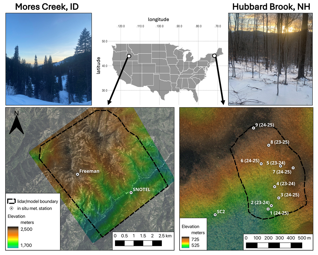
Figure 1 Map of study areas. Including a map of the U.S. (top) with each site indicated and a representative photo taken from within each basin. To the left is Mores Creek in Idaho, U.S., and to the right is Watershed 3 in Hubbard Brook Experimental Forest in New Hampshire, U.S. Ground-based “in-situ” meteorological observation sites are indicated. At Mores Creek, two sites are included at a lower (SNOTEL) and upper elevation (Freeman). For Hubbard Brook Watershed 3, nine observational locations are included within the basin and labeled based on their relative elevation, ranging from lowest (1) to highest (9). An additional site, SC2, marks a long-term snow course transect (1956–present) and meteorological site. Lower row imagery © 2025 NASA/Copernicus, Map data © 2025 Google. Photos taken by Jeremy Johnston.

2 Study Areas

2.1 Mores Creek, Idaho, USA

The Mores Creek basin (43.96° N,115.69° E) is an approximately 35 km² mountainous basin in southwestern Idaho. The site encompasses a range of snow climates (Sturm and Liston, 2021), including persistent montane and boreal forest snowpacks at high elevations and transitional snow sagelands at lower elevations. As such, a wide range of peak snow depths is represented from shallow snow in forested or exposed areas (<0.5 m) to deep snow up high and in drifts that often exceed 3 m in spring. The upper basin survey area contains approximately 600 m of topographic relief distributed across all aspects and a mean elevation of 2100 m. Topography is complex, with deeply incised ravines and no preferred orientation of valleys and ridges. Snow tends to be present from November to May, with peak depths occurring in late March or early April. The 30-year average peak snow depth at the Mores Creek Summit SNOTEL is 2.3 m (site 637; https://wcc.sc.egov.usda.gov/nwcc/site?sitenum=637, last access: 16 June 2025). The entire domain is below treeline, and is forested primarily with conifers (Spruce, Pine, Fir). Approximately 40 % of the lidar domain was burned in the 2016 Pioneer fire (moderate severity).

2.2 Hubbard Brook, New Hampshire, USA

Hubbard Brook Experimental Forest (43.96° N, 71.72° E) is an approximately 32 km² research basin-situated in the White Mountains of New Hampshire. In this study, we focus on Watershed 3 (hereafter referred to as Hubbard Brook), a small 0.42 km² (∼100 acres) sub-basin within Hubbard Brook. The snowpack in Hubbard Brook is part of the transitional montane forest snow climate (Sturm and Liston, 2021; Johnston et al., 2026) and is considered representative of many snowpacks in forested regions within the northeastern United States. Snow depths in Hubbard Brook are generally moderate to shallow (<1 m),but may exceed 1 m during snowy seasons. Differences in forest cover, aspect, and elevation are known to drive gradients in snow depth, which are generally small across Watershed 3 (<0.25 m). The basin has an elevation range of approximately 200 m from the outlet (520 m) to the ridgetop (718 m). There are two distinct aspects in the basin: the western side, which is south-facing, and the eastern side, which faces southwest. The snowpack typically establishes in late November and melts out by mid-April. The 30-year average peak snow depth is 0.6 m (site STA2/SC2; https://portal.edirepository.org/nis/mapbrowse?packageid=knb-lter-hbr.27.20, last access: 16 May 2025). The basin is mostly deciduous forests ranging in height from 15 to 30 m, with shorter mixed and conifer forests (10 to 15 m) prevalent in the upper elevations of the basin.

Together, these basins span a strong west–east contrast in snow and terrain regimes. Mores Creek is a larger, high-relief, wind-affected western basin with deep, persistent snow and pronounced redistribution. In contrast, Hubbard Brook is a smaller, lower-relief, transitional northeastern forested basin with shallower, more spatially uniform snowpacks and milder temperatures.

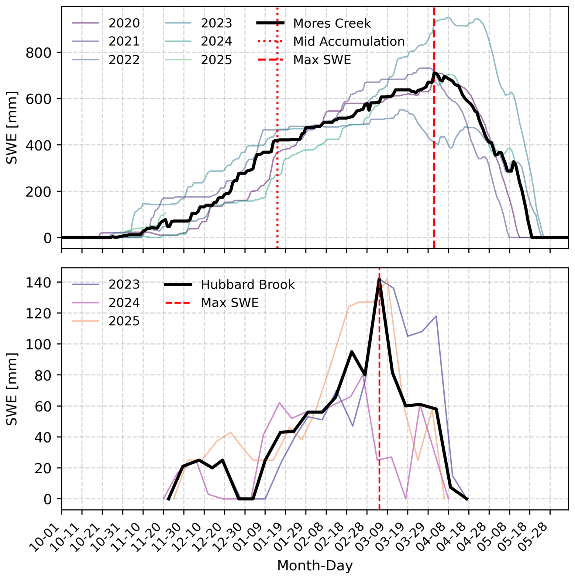
Figure 2 Summary of snow water equivalent (SWE) records for Mores Creek (top) and Hubbard Brook (bottom). Solid black lines represent the median SWE, while colored lines denote individual trajectories each winter. Vertical dashed and dotted lines indicate critical seasonal transition points, including mid-accumulation and maximum annual SWE.

2.3 Snow season phases

To align model evaluation and residual analyses with the physical progression of the snow season across domains, from accumulation to peak to melt, we identified seasonal phases for each site. The seasonal phases are delineated in Fig. 2 and associated with each lidar flight, showing that all seasonal phases are well represented at each study area (Table A1).

Winter phases were defined using site-specific SWE climatologies. At Mores Creek, 2019–2025 SNOTEL data identified a mean peak SWE date of 2 April and an accumulation midpoint of 16 January, delineating three periods: early (accumulation; N=5 lidar surveys), middle (peak storage; N=8), and late (ablation; N=5). At Hubbard Brook, the transitional snowpack necessitated a two-phase division: early-mid (accumulation; N=8) and mid-late (ablation; N=8), separated by a March 6 peak storage date. This threshold reflects the near-term (2023–2025) average while accommodating the coarse resolution of weekly sampling intervals. To ensure balanced sample sizes across these two phases, two acquisition collected on 1 March 2024 and 3 March 2025, were classified into the mid-late phase despite occurring marginally before the climatological peak.

3 Data

3.1 Lidar surveys

Lidar surveys (detailed in Table A1) at each site were used to derive high spatial resolution (<1 m) snow depth maps and static geospatial predictors from digital terrain and canopy height models (CHM) for use in the RF modeling workflow (see the next section).

3.1.1 Mores Creek Lidar surveys

Airborne helicopter lidar surveys were conducted multiple times per year from spring 2020 to 2025 over the ∼35 km² Mores Creek domain in the Boise Mountains of central Idaho to monitor headwater snow distribution. Flights were performed with a helicopter-mounted sensor pod consisting of Riegl VQ-580 ii Airborne Laser Scanner, an Applanix AP60 Inertial Measurement Unit (IMU), and an Antcom G5ANT-42AT1 GNSS Antenna. Semi-permanent GNSS base stations are used during processing to optimize the helicopter trajectory, and each survey includes a boresight collection over a subdivision which is used to ensure IMU orientation parameters are correctly calibrated due to the external and removable nature of the scanner system. Collections average 30–40 ground returns per m² with ∼10 cm accuracy. A snow-free acquisition collected by NV5 Geospatial serves as a reference map from which snow-on flights are differenced to isolate snow depth (Adebisi et al., 2022). A total of 18 snow depth maps were acquired during this period. Snow depth for each survey was calculated by differencing processed digital terrain models between a snow-off baseline flight and the corresponding snow-on flight (Ciafone et al., 2024) after manual proprietary processing (Riegl, RiProcess) and automated batch processing using an in-house codebase (https://github.com/cryogars/ice-road-copters, last access: 16 June 2025). This software mosaics, filters, co-registers and rasterizes (1 m) point cloud data (Hoppinen et al., 2023). Surveyed snow depths ranged from 0 to more than 4 m, with an average depth of approximately 150 cm and standard deviations around 50 cm (Table A1).

3.1.2 Hubbard Brook Lidar surveys

A series of Uncrewed Aerial System (UAS) lidar surveys was conducted throughout the 2023–2024 and 2024–2025 winter seasons at Hubbard Brook's Watershed 3 (WS3). The flights covered the entirety of the gauged drainage basin. UAS-lidar observations were used to produce high-resolution snow depth estimates by subtracting bare-earth digital elevation models (DEMs) from snow-on elevation models, following the methodology in Jacobs et al. (2021). The DEM workflow consisted of trajectory refinement, strip alignment, outlier removal, and ground classification. Bare-earth and snow-on points clouds were gridded at 0.5 m using only ground-classified lidar returns to produce the DEMs. Each survey was matched to the reference bare-earth grid using bilinear interpolation prior to differencing. The resulting dataset consists of four UAS lidar snow depth maps from the 2023–2024 winter season and 12 snow depth maps from the 2024–2025 winter season.

For the surveys conducted in 2023–2024, the UAS sensor package used was the LiAirV70 manufactured by Green Valley International. The system integrates the Livox Avia laser scanner with a Notel IMU (Attitude accuracy: 1σ of 0.008°, Azimuth accuracy: 1σ of 0.038°). All flights were conducted at an altitude of 40 m above ground level and a flight speed of 2.5 m s⁻¹. Collections using the LiAirV70 averaged approximately 30 ground returns per m². These flight parameters were selected to maximize the accuracy of both the laser scanner range measurements and the positional/attitude measurements from the IMU. A 50 % overlap was used to determine flight line spacing. For the 2024–2025 WS3 surveys, the MiniRanger3, manufactured by Phoenix Lidar Systems, was used to enhance UAS lidar collection efficiency. The MiniRanger3 integrates the Riegl miniVux3 lidar and the NovAtel OEM7 INS. This hardware enabled data collection at higher flight altitudes (80 m) and faster flight speeds (8 m s⁻¹) while maintaining high positional accuracy and sufficient lidar ground return density (averaged approximately 50 ground returns per m²). The flight trajectories measured by both the LiAirV70 and miniRanger3 were post-processing kinematic (PPK) corrected. This was done using an Emlid Reach RS2+, which sampled GNSS observables at a frequency of 1Hz throughout the duration of each flight. A monument with known coordinates (±5 cm) was established prior to each winter season, and the Emlid was placed over the monument for each flight to ensure UAS mapping products were correctly aligned. The precise location of the monument was established by collecting 10+ h of GNSS observations over the monument location and post-processing that data through the NOAA Online Positioning User Service (OPUS) web service. Surveyed snow depths ranged from 0 to nearly 1 m, with an average depth of approximately 30 cm and standard deviations around 10 cm (Table A1).

3.2 Derived static variables

From the snow-off baseline flights from Mores Creek and Hubbard Brook, we derived static predictors from digital terrain and canopy height models (CHM), including elevation, aspect, northness, eastness, slope, topographic position index (TPI), and proximity to trees to capture terrain controls on snow accumulation and melt. CHMs were calculated by differencing digital surface models (surface elevations including tree top elevations) and digital elevation models (ground-classified elevations only). TPI is an index that defines the relationship of a pixel's elevation to its neighbors (Reu et al., 2013). Positive TPI values indicate local points higher than their surroundings, and negative values indicate lower areas like valleys and depressions. TPI was calculated using the 3×3 neighborhood around each pixel (1.5×1.5 m). We also calculated northness and eastness as the cosine and sine of aspect, in radians, respectively. These two variables range from 1 to −1 and indicate how strongly a slope faces north to south or east to west, capturing exposure to sun and prevailing winds. We calculated a terrain-based snow redistribution index using a combination of upwind slope, wind factor, and accumulation factor (Winstral and Marks, 2002). Upwind slope was computed for each DEM cell as the maximum slope toward the upwind terrain within a 200 m search distance, stepping every 2.5 m for azimuth windows centered every 60° with a ±25° window. Upwind slopes were aggregated into a mean value for each pixel. This slope was linearly scaled to a wind factor ranging from 1 (sheltered) to 2.3 (exposed), and the accumulation factor was derived as the inverse of wind factor to represent deposition potential. Redistribution was then calculated as the product of wind factor and accumulation factor, with higher values indicating drift zones and lower values representing wind-scoured areas. Forested pixels derived from the CHM were assigned a wind factor of 1 in Mores Creek, increasing the redistribution in sheltered forest zones to reflect enhanced snow deposition. This modification was not applied to Hubbard Brook wind factor maps, because it is more than 95 % forested. Unlike the upwind slope alone, the redistribution index accounts for both terrain exposure and deposition potential, providing a more complete indicator of wind-driven snow redistribution in complex terrain.

3.3 Meteorological and in-situ snow data

3.3.1 Mores Creek in-situ observations

Two in-situ stations within the Mores Creek domain collect daily snow depth measurements (Fig. 1). The Mores Creek Snow Telemetry (SNOTEL) station, situated at 1853 m in a more accessible location, provides daily records of snow depth, snow water equivalent (SWE), temperature, and wind speed and direction for the full period of record. In this study, SNOTEL observations are used for both model training and evaluation. Freeman Station, located near the summit of Freeman Peak at approximately 2393 m, provides snow depth data only for the 2024–2025 winter season. These measurements are used solely for model validation, providing an independent check at a higher elevation site not used to drive the model.

3.3.2 Hubbard Brook in-situ observations

A long-term meteorological station less than 1 km from the centroid of WS3 (SC2, Fig. 1) was used as the in-situ source data to train RF models and to establish a SWE and snow depth climatology for the site. Nine meteorological sites within Hubbard Brook WS3 collected sub-daily snow depth measurements during the 2023–2024 (4 sites) and 2024–2025 (6 sites) winters. Site 8 was maintained during both winters, while the other sites differed between winter 2023–2024 and 2024–2025. Site numbering indicates the winter in which each site was operational and its relative elevation (1 – lowest, 9 – highest). Snow depths at these sites were retrieved from time-lapse imagery at least 3× daily using a demarcated (5 cm increments) snow stake. Stake coordinates were surveyed using a high-precision Emlid RS 2+ GPS system (±20 cm) for validating modeled snow depth estimates.

3.3.3 ERA5-Land Reanalysis

Daily ERA5-Land reanalysis time series were acquired for snow depth, air temperature, and the U and V wind components (Muñoz Sabater, 2019). ERA5-Land has a native spatial resolution of ∼9 km; the Mores Creek domain encompasses four grid cells, and Hubbard covers a single grid cell. For Mores Creek, we averaged the four ERA5-Land pixels to produce a single daily value for each variable. Wind speed and direction were derived from the U and V wind components. Daily wind speed was computed as:

$$\begin{array}{}\text{(1)}& \text{wind\hspace{0.17em} speed}=\sqrt{(U^{\mathrm{2}}+V^{\mathrm{2}})}\end{array}$$

and wind direction (in degrees from north) as:

$$\begin{array}{}\text{(2)}& \text{wind\hspace{0.17em} direciton}={\tan }^{-\mathrm{1}}\left({\displaystyle \frac{U}{V}}\right)\times \left({\displaystyle \frac{\mathrm{180}}{\mathit{\pi }}}\right)\end{array}$$

Negative directions (−180 to 0°) were converted to the 0–360° meteorological convention by adding 360° to negative values to produce a single daily wind vector representing the average wind conditions over the domain.

4 Methods

4.1 Random Forest snow depth modeling framework

The RF modeling framework was designed to test whether sparse lidar acquisitions can be extended into continuous seasonal snow depth maps when combined with static terrain and land cover variables and dynamic daily meteorological data. In our experiments, this daily forcing is provided either by in-situ stations (SNOTEL and SC2) or by ERA5-Land reanalysis and includes timeseries of snow depth, air temperature, and wind, which act as the temporal driver for the RF. This approach enables interpolation between flight dates to generate daily snow depth time series suitable for cross-seasonal analysis and potential operational monitoring. RF was chosen for its ability to capture complex, nonlinear relationships between snow depth and physiographic or meteorological predictors, and for its robustness to overfitting in high-dimensional feature spaces (Breiman, 2001). All RF training, validation, and hyperparameter tuning were performed independently for each domain (Mores Creek and Hubbard Brook).

4.1.1 RF model setup

The target variable was lidar-derived snow depth (m), predicted for each valid pixel and day. Valid pixels were considered as those with lidar snow depth observations for all dates at Mores Creek (N=18). In Hubbard Brook, pixels with valid depth observations in at least 15 (of 16) flights were considered valid for model training. This was due to a one flight (2 February 2024) in which observations were only collected over half of the basin. For both domains, model training and evaluation were conducted strictly within a defined parameter space of valid pixels to ensure that the RF model operated under conditions represented in the training data. Working within parameter space is critical for RF because its decision-tree structure performs best when interpolating within the bounds of observed predictor values, whereas predictions outside that space risk being unreliable (Reichstein et al., 2019). In the Mores Creek domain, a pixel was included in the parameter space only if it appeared in every lidar acquisition, was located outside a two-meter buffer of Highway 21 and did not exceed the 99.99th percentile of observed snow depth across the full lidar record. Similar considerations were applied at the Hubbard Brook site, using only observations within the watershed boundary and outside of a two-meter buffer of a frequently traversed trail within the basin.

A consistent equal-allocation stratified sampling framework was applied across sites to generate training data. Aspect was reclassified into four cardinal classes (north, east, south, and west), and elevation was divided into four quantile-based bins derived from a DEM, producing up to 16 strata. An equal number of pixels was sampled from each stratum within a valid-pixel mask, with total sample sizes scaled to basin extent (50 000 pixels at Mores Creek and 10 000 at Hubbard Brook). This ensured comparable sampling density and minimized the influence of domain size on model behavior. At Mores Creek, the stratified sample size represented roughly <0.25 % of all valid pixels and spans all combinations of elevation and aspect classes, while at Hubbard Brook the stratified samples similarly cover the full elevation-aspect range.

RF snow depth models are known to have limited predictive capacity for unseen conditions and struggle to properly account for meteorology-driven snow accumulation and ablation processes (Revuelto et al., 2020). Recent literature has indicated that predicting snow depth in terms of residuals relative to a in-situ reference site (i.e., source) is more effective than direct predictions of snow depth (Herbert et al., 2025). During model development, we tested models directly predictive of both snow depth and relative snow depth, defined as:

$$\begin{array}{}\text{(3)}& \begin{array}{rl}\text{Relative snow depth}& =\text{lidar observed snow depth}\\ & -\text{source snow depth}\end{array}\end{array}$$

We found that relative snow depth models produced more cohesive and temporally realistic estimates of snow depth. Thus, the RF models presented herein were trained to predict relative snow depths. With this approach, areas observed to be deeper than the reference data (e.g., source) are assigned a positive value, while those observed to be shallower than the reference are assigned a negative value. In other words, the RF model is used to learn appropriate spatial bias corrections (as observed by the lidar) relative to existing snowpack observations (i.e., in-situ) or model estimates (i.e., source via ERA5-Land).

In total, we used nine (9) static predictors, including elevation, slope, aspect, TPI, northness, eastness, CHM, proximity to trees, and the terrain-based redistribution index following Winstral and Marks (2002). An additional seventeen (17) dynamic predictors were derived from daily in-situ observations, including air temperature, snow depth, and wind speed and direction, with daily wind vectors calculated from the U and V components. Together, these predictors capture many of the physiographic and meteorological controls on snow accumulation and melt. Day of the water year (DOWY), starting on 1 October, was also used. For DOWY, air temperature, and snow depth lag (3, 5 d prior) and lead (3, 5 d in the future) were added to provide the model with temporal context.

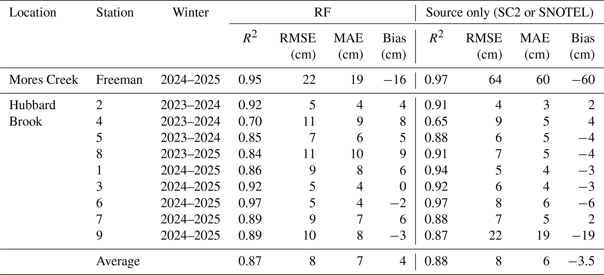
Table 1 Performance statistics using RF models driven by in-situ data (RF) versus direct application of independent in-situ observations (source only). For Hubbard Brook, the average is the weighted average of all sites based on the number of observations collected at each site.

To further guide the model in representing the full seasonal cycle, we introduced synthetic snow depth maps generated as spatially uniform grids where snow depth was set to zero across the entire domain. These zero-value maps were assigned to specific dates at the beginning (before the first snowfall) and at the end (after snowmelt) of each winter season and paired with the actual meteorological forcing data for those days. These synthetic maps constrained the model to recognize periods of no snow, providing clear lower bounds for snow accumulation and melt. By anchoring the seasonal ends of predictions, these synthetic observations reduced uncertainty around the start and end of the winter, helping the RF model transition smoothly between snow-covered and snow-free periods.

The RF model, using the RandomForestRegressor object in Python's Scikit-learn library (Pedregosa et al., 2011), was hyper parameterized using a cross-validated grid search to identify the optimal combination of number of trees (100, 200, 300), maximum depth (10, 20, 30), minimum samples for splits (2, 5, 10) and leaf nodes (1, 2, 4), and maximum features per split method (“auto”, “sqrt”, “log2”) that minimized prediction error while limiting overfitting (Table A2). Model training and evaluation followed an 80/20 train/test split of lidar acquisition dates, repeated over ten iterations to quantify variability in model performance. Model skill was assessed using R², root mean square error (RMSE), mean absolute error (MAE), and bias. Once trained, the model was applied to generate daily snow depth maps for all valid pixels, bridging the periods between lidar flights to form a continuous seasonal record.

4.1.2 RF model evaluation

Trained RF models were assessed using three different approaches. The first (“Training evaluation”), described above, employed 80/20 training/test splits to evaluate the model's ability to capture observed patterns at each site, using only data from dates with lidar observations. The second (“Independent time series evaluation”) compared daily RF predictions with time-series observations from independent ground-based in-situ sites, using a small buffer (∼1 m) around each in-situ observing location to extract corresponding RF predictions. For the RF model in Mores Creek, only one site (Freeman) and the 2024–2025 winter were used for this time-series evaluation, because SNOTEL observations are used as the temporal driver and cannot simultaneously serve as an independent validation series. Freeman thus provides an independent, high-elevation check on the in-situ driven RF model, while SNOTEL is used over multiple years as an independent reference when evaluating the ERA5-driven RF model (Sect. 5.3, Table 1). At Hubbard Brook, time-series evaluations were conducted at each of the nine in-situ sites across 2023–2025, providing a multi-site, multi-year assessment of temporal performance (Table 1).

The final evaluation was conducted using spatial error maps (RF predicted – lidar). This analysis compared RF predictions generated for the full domains on each date with lidar acquisitions to the lidar observations themselves; for each comparison date, an RF was trained using the described framework but with observations from that prediction date excluded from the training data. Metrics R², RMSE, MAE, and bias were used to quantify model performance for each of the three evaluation methods.

4.1.3 Error Distribution

To characterize model performance beyond global statistics, spatial error maps (i.e., model residuals) were evaluated across terrain and land cover gradients. To quantify the influence of these physiographic variables on error distributions, we conducted one-way analysis of variance (ANOVA) (Stahle and Wold, 1989) tests with residuals binned by Jenks natural breaks for continuous variables (e.g., slope, elevation, redistribution) and by cardinal classes for aspect. Results were aggregated by averaging the explained variance (R²) outputs for each topographic or vegetation predictor across all snow season phases. This highlighted which terrain features most strongly controlled model error and whether these patterns were consistent across accumulation and melt periods.

4.1.4 RF model predictor importance

Shapley Additive exPlanations, also termed Shapley values or “SHAP” scores (Lundberg and Lee, 2017), were used to measure the explanatory value of all predictors used in the RF model and identify which inputs exert the largest influence on RF model predictions. The SHAP method measures the predictive influence of each input feature across a large ensemble of individual model predictions in the prediction units (e.g., cm). Due to the large size of the RF training dataset, input feature sets were sub-sampled by randomly selecting 10 feature sets (containing all 26 predictors) from 10 equal-interval bins of each predictor. This resulted in a diverse yet equally weighted sample of input predictor feature sets, enabling the efficient calculation of SHAP scores. The distribution of all SHAP scores is provided along with average absolute SHAP scores for each predictor variable to provide a single summary measure of predictive influence.

4.2 Experiments

4.2.1 Lidar drop date analysis

To evaluate how lidar acquisition frequency influences predictive skill, we conducted a drop-date analysis using the same equal-allocation stratified sampling framework drawing 50 000 pixels at Mores Creek and 10 000 pixels at Hubbard Brook (due to its smaller size) for model training. In each iteration, one lidar acquisition date was randomly selected as the prediction target and withheld from the training set. From the remaining acquisitions, an increasing number of dates were randomly dropped to simulate sparser campaigns. The model was trained on all remaining dates and used to predict the withheld date, with performance evaluated using R², RMSE, MAE, and bias. This process was repeated for 100 iterations per drop scenario, capturing variability due to random selection of prediction and drop dates and identifying the point of diminishing returns for lidar frequency. Drop scenarios ranged from using data from all dates except the withheld date for training (N−1, where N is the total number of lidar maps) to using only a single randomly selected map for training the model (N=1, training on one date and predicting on another). Non-parametric Kendall's tau coefficients and p-values were calculated to determine the significance of the relationship between the number of lidar maps used and RF prediction errors (Kendall, 1962). The target prediction dates were then used to bin the results into the early, middle, and late phases for Mores Creek and into early-mid and mid-late phases for Hubbard Brook using the methods outlined in “Snow season phases”. This analysis quantified whether models trained during accumulation could reproduce melt-season snow distributions (and vice versa).

4.2.2 Cross-phase analysis

To test seasonal transferability, we also used the seasonal phases to partition observations by phase for training and testing of the RF snow depth models. For each experiment, the RF model was trained on all lidar acquisitions from a source phase and evaluated for a single randomly chosen date within the target phase, ensuring no target-phase data were used in training. Each source-target combination was repeated for 10 iterations, and the results were summarized using the average R², RMSE, MAE, bias, and the observed snow depth on the target date. This was used to calculate the error relative to observed snow depths at a given site and period, due to the large range in conditions captured within and across sites. The same sampling procedure as in the drop analysis was used to identify pixels for model training and testing

4.2.3 ERA5-Land vs. in-situ evaluation

In a separate experiment, we tested whether ERA5-Land reanalysis could supplement or replace in-situ meteorological observations (air temperature, snow depth, wind) to support snow depth prediction in data-sparse basins. ERA5-Land is a reanalysis dataset that provides daily meteorological variables across global land areas (Muñoz Sabater, 2019). It is widely considered among the most accurate, especially for snow applications (Mortimer et al., 2020), and can provide estimates of snow depth and SWE in the absence of local in-situ data (Alonso-González et al., 2022).

To assess the feasibility of using ERA5-Land as an alternative forcing source, we repeated the RF training workflow using ERA5-Land variables for air temperature, wind speed and direction, and snow depth. We then re-applied the time series evaluation procedure. Specifically, the ERA5-Land–driven RF model was used to generate daily snow depth time series for each year, from which modeled values were extracted at in-situ station locations and compared against observed measurements. Further evaluation involved producing modeled snow depth for 10 000 randomly selected pixels within the Mores Creek basin using both the SNOTEL- and ERA5-Land–driven models. The same procedure was applied at Hubbard Brook, except across the full domain. The resulting aggregated time series from each model were compared, and performance metrics including the R², RMSE, MAE, and bias were calculated.

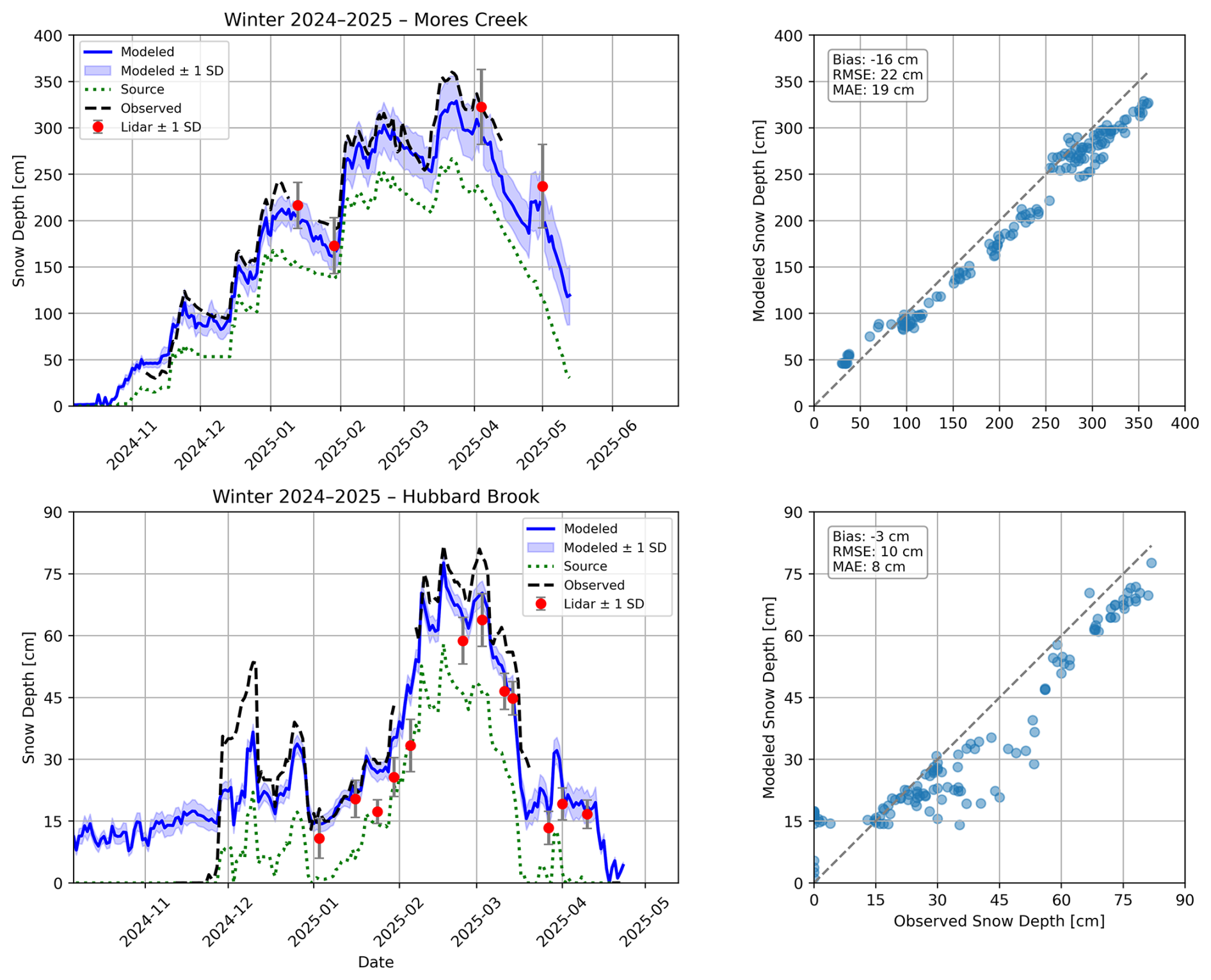
Figure 3 Point-scale time-series comparison between the RF model (Modeled) and independent snow depth observations (Observed). Evaluation uses observations from the Mores Creek Freeman site (top) and the Hubbard Brook site 9 (bottom). Source refers to the source snow depth data used in the relative depth calculation for Mores Creek (SNOTEL) and Hubbard Brook (SC2). Performance statistics are summarized in Table 1.

5 Results

5.1 RF snow depth model performance

5.1.1 Training evaluation

The RF model trained on all dates and evaluated using an 80/20 train/test split repeated over 10 iterations showed consistently high predictive skill for daily snow depth mapping in both study domains. The 80/20 split results provide comparisons between model predictions and lidar-derived snow depth at the pixel scale, representing spatial prediction accuracy summarized across the full study spatial domain and time period. On average across the 10 iterations, the RF model at the Mores Creek site explained 89 % of the variance in observed snow depth with a MAE of 18 cm (12 % of mean snow depth). RMSE averaged 28 cm (18 %), indicating strong agreement between predicted and lidar-observed snow depth across diverse terrain and snow conditions. Performance at the Hubbard Brook site was similarly high, with the model explaining 90 % of the variance in observed depth and RMSE and MAE values of 7 cm (23 %) and 5 cm (19 %), respectively. This demonstrates the RF modeling framework's ability to reproduce daily snow depth patterns using individual models trained across contrasting western and eastern snowpack regimes.

5.1.2 Independent time series evaluation

We also evaluated the model against independent in-situ snow depth observations from Freeman Station in the Mores Creek domain and from the nine stations in the Hubbard Brook model domain, providing a temporally focused point-scale assessment. Daily time series predictions compared to Freeman station observations produced a bias of −16 cm, an RMSE of 22 cm, and an MAE of 19 cm (Fig. 3). This was a sizeable improvement relative to assuming observed conditions at the SNOTEL (source) alone were representative of snow depth conditions at Freeman (bias: −60 cm, RMSE: 64 cm, and MAE: 60 cm), demonstrating the ability of the RF to integrate both temporal (SNOTEL) and spatial (lidar) information for improved daily depth estimates. The in-situ record for this site is limited to a single season (2024–2025) and ends on 8 April 2025, when the station stopped reporting data. Despite this truncated record, results indicate the model maintained low bias and strong agreement with an independent point-scale measurement

For Hubbard Brook, model performance was validated across two separate winters of time-series snow depth observations (2023–2024 and 2024–2025, Table 1), achieving strong average performance across all sites (R²: 0.87, RMSE: 8 cm, MAE: 7 cm, bias: −4 cm). In 2023–2024, for four sites, RMSE ranged from 5 to 11 cm, and bias was slightly positive (+4 to +9 cm). In winter 2024–2025, performance across six independent sites was similarly high, with equivalent RMSE to 2023–2024 (5 to 11 cm) and bias ranging from −4 to +9 cm. As shown for site 9 in Fig. 3, there was a noted model high bias when snow depth was observed to be 0 cm in the early season. We hypothesize that because the source data came from a location where the snow was shallower and melted out earlier than at site 9 (site SC2), a positive snow depth bias persists in the model. This effect occurred to varying degrees, +5 to +15 cm at sites with deeper or more persistent snow than SC2 (sites 3–9) and was negligible at sites shallower than SC2 (sites 1 and 2). Averaged across sites and years, the RF model provided no improvement over using nearby in-situ snow depth observations (SC2) to predict snow depth. While at most locations, mean absolute errors using SC2 were within 5 cm, the value of the RF model was apparent in the deepest snow (site 9), where the RF approach improved RMSE and MAE by more than 10 cm and reduced bias from −19 to −4 cm.

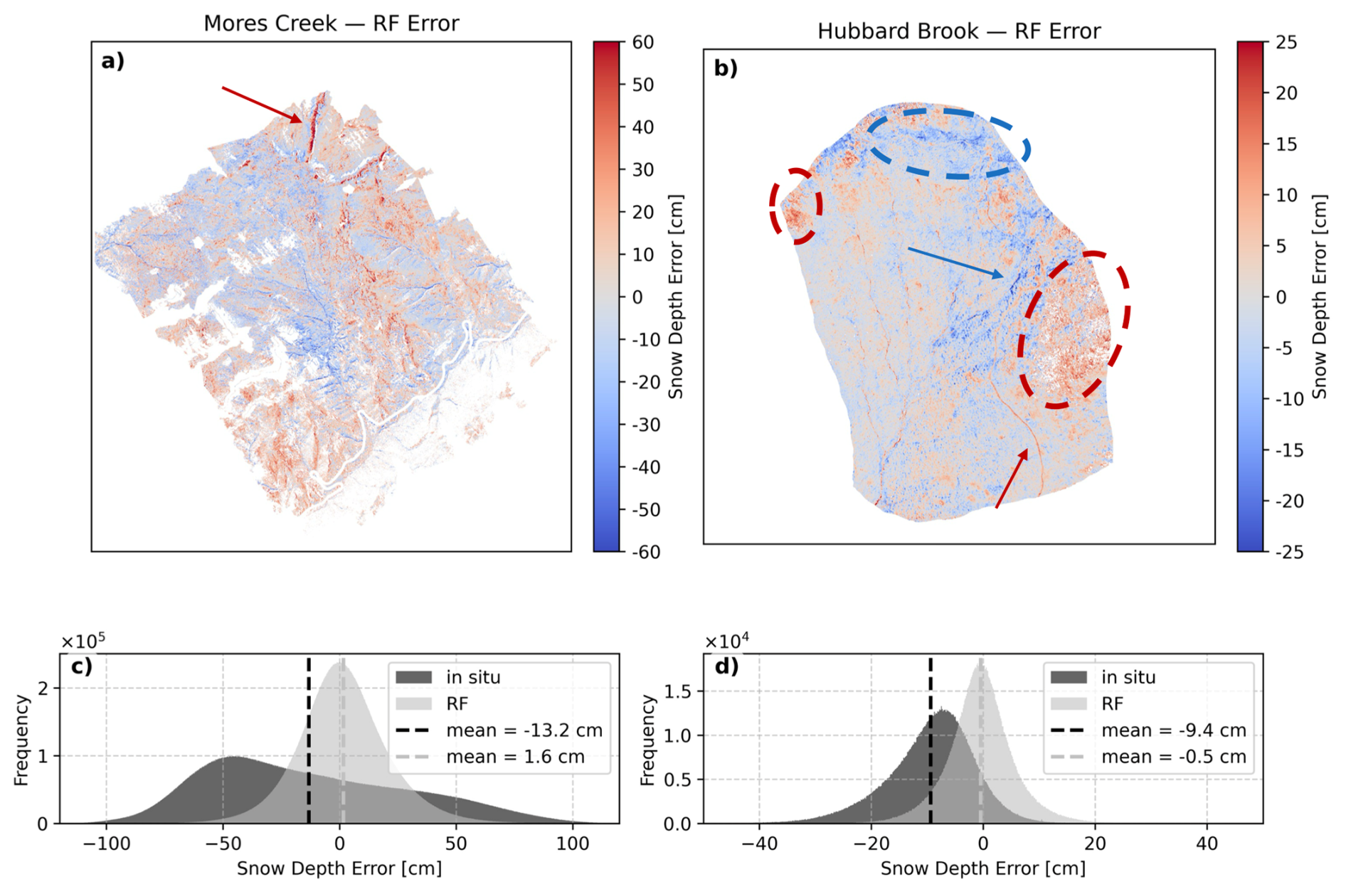
Figure 4 Spatial distribution of averaged model residuals (RF prediction – lidar observation, light grey) for (a) Mores Creek and (b) Hubbard Brook. Histograms comparing the RF model errors across the basin (light grey) against the distribution of differences when assuming the basin-wide snow depth is equal to the in-situ station observation (dark grey) are shown for (c) Mores Creek and (d) Hubbard Brook. Arrows and circled areas indicate noted areas of model overprediction (red) and underprediction (blue).

5.1.3 Evaluation of model spatial error, and bias

To evaluate accuracy in space, snow depth maps were predicted for each day having lidar snow depth observations using the RF model trained on lidar acquisitions from all other dates. The average snow depth residuals (RF prediction minus lidar observation) were mapped to show the spatial distribution of model errors (Fig. 4). Over most of both domains, there are relatively small prediction errors (<25 cm), with only a small fraction of pixels showing larger deviations. At Mores Creek, there is a low overall spatial bias of 1.6 cm, with 44.0 % of pixels within ±10 cm, 81.8 % within ±25 cm, and 97.8 % within ±50 cm of observed values. At Hubbard Brook, the model spatial bias was −0.5 cm, and 90.0 % of pixels fell within ±10 cm of the actual value. Nearly all predictions (99.8 %) at Hubbard Brook were within ±25 cm.

At Mores Creek, a localized area of higher error values occurred along a prominent cornice feature in the upper basin, where wind redistribution frequently alters snow depth patterns in ways that are not fully captured by the model predictors (red arrow, Fig. 4a). In Hubbard Brook, overpredictions were common within areas of coniferous forest cover (indicated by red circles). Snow tended to be underpredicted in higher elevation areas (blue circle) and in steep, sheltered terrain features (blue arrow). The model also overpredicted snow depths for a packed access trail (red arrow, Fig. 4b) and in streambeds.

To isolate the value of the spatial modeling approach, the distribution of mean residuals from the RF model (light grey) was compared against a baseline assumption where the local in-situ snow depth is uniformly applied across all pixels in the basin (dark grey; Fig. 4c and d). At Mores Creek, this in-situ baseline approach (using SNOTEL daily snow depth) resulted in a basin-wide difference of −13.2 cm, regularly underestimating deep snow areas by more than 50 cm (Fig. 4c). At the Hubbard Brook basin, the in-situ baseline (using SC2 daily snow depth) showed a basin-wide difference of −9.4 cm, underestimating snow depth in 91 % of pixels. This comparison highlights a key takeaway: the assumption that a single in-situ station is representative of basin-wide snow distribution is significantly more consequential at the larger, more topographically complex Mores Creek site than at the smaller Hubbard Brook site. Still, this assumption can break down at relatively small scales (<1 km²), as shown by local differences exceeding −30 cm at Hubbard Brook (Fig. 4d). In contrast to the baseline assumptions, the RF models successfully corrected these discrepancies across both sites, proving generally unbiased (bias within ±2 cm) with an even distribution of positive and negative average residuals (Fig. 4d).

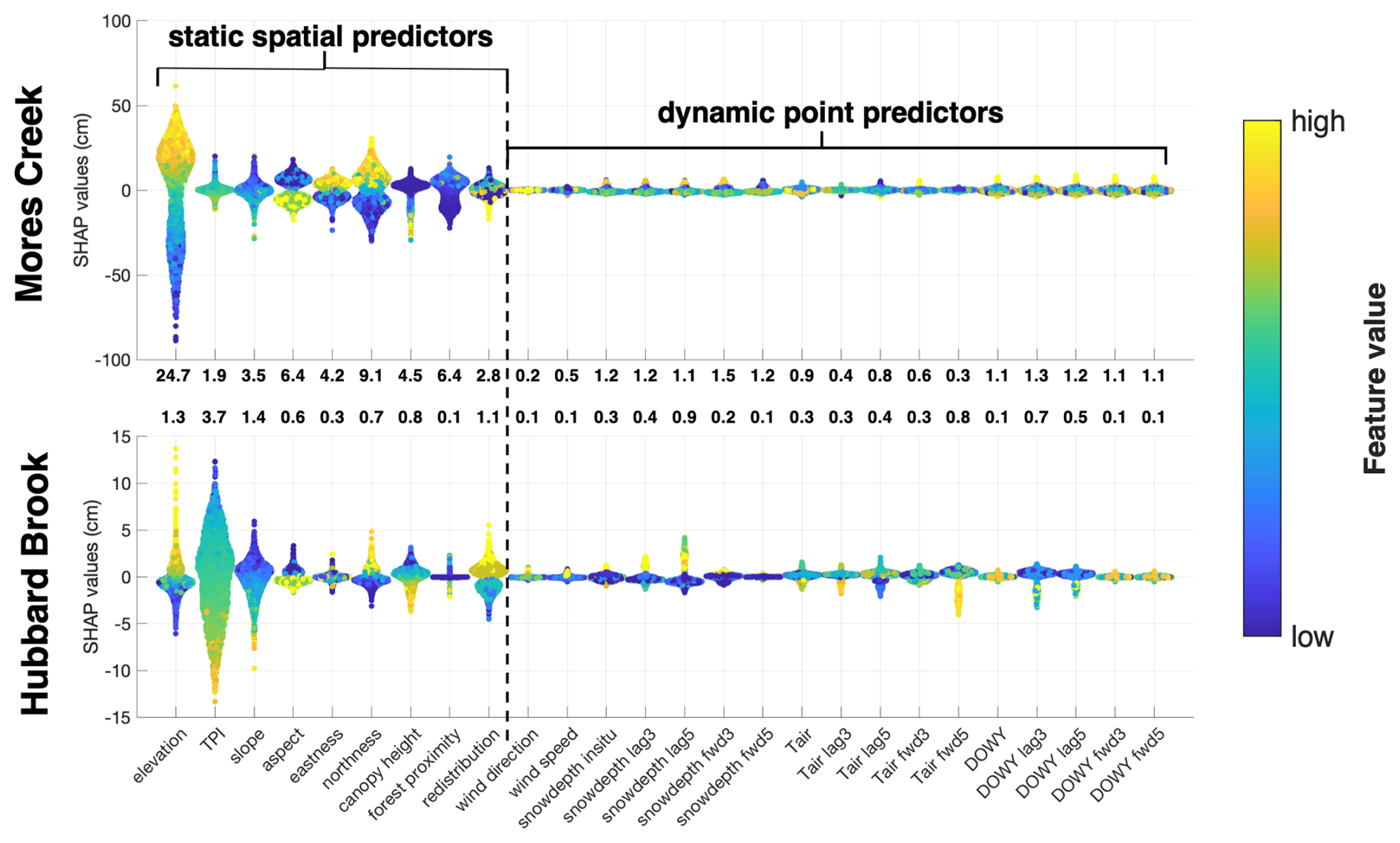
Figure 5 SHAP RF model feature importance by study site. Bolded numbers are the average absolute SHAP score; all units are cm. The left-most variables include geospatially derived predictive features, and the right-most are those derived from meteorological observations collected at a single in-situ site near each study area. Note the different y-axis ranges due to different snow depth variability values observed at each site (Table A1).

5.1.4 Model predictor importances

The SHAP analysis for the Mores Creek and Hubbard Brook RF snow depth models quantified the contribution and direction of influence for all model predictors across sites. At both sites, static spatial predictors (e.g., elevation) were notably more crucial to model predictions than dynamic point predictors derived from meteorological observations, including snow depth (Fig. 5). At both sites, the SHAP analysis agreed with the expected physical relationships between predictors and snow depth finding that increasing TPI, slope, and canopy height generally decreased snow depth. Conversely, increasing elevation, northness, and redistribution indices resulted in increased snow depth. This likely reflects a confounding relationship between elevation and forest canopy heights in both study areas, in which forests are taller and more common at lower elevations relative to high elevations, but may provide insight as to the influence of forests on snow accumulation.

While dynamic predictors provided minimal predictive value, higher relative DOWY values generally increased predicted snow depth at Mores Creek. Whereas high 5 d forward-looking air temperatures (“Tair fwd5”) generally decreased in modeled snow depth, and deeper 5 d backward-looking snow depths (“snowdepth lag5”) slightly increased modeled snow depths, at Hubbard Brook. Although most dynamic predictors have lower SHAP importance than static terrain variables, we retained them for two reasons. First, some dynamic features (DOWY, forward-looking air temperature, lagged snow depth) exert seasonally dependent influences on model predictions. Second, part of our goal was to quantify their contribution relative to terrain and canopy predictors within a single model, rather than to derive a pared-down model. Future applications could prune or simplify this dynamic predictor set to improve interpretability and transferability once the relative contributions of these variables are established.

In Mores Creek, elevation was the single most important predictor (mean absolute SHAP value: 24.7 cm), with increasing elevation generally increasing the magnitude of snow depth predictions in the RF model, as shown by the blue (low elevation values, down to −100 cm) to yellow (high elevation values, up to +50 cm) gradient in Fig. 5. Northness (9.1 cm) and aspect (6.4 cm), as well as forest proximity (6.4 cm), had the next highest influence on model predictions. Reinforcing that terrain orientation and wind redistribution processes are linked to spatial error patterns.

In Hubbard Brook, lower snow depths and less diverse snow depth conditions resulted in a smaller relative SHAP importance for all spatial metrics. Still, TPI (mean absolute SHAP: 3.7 cm), slope (1.4 cm), elevation (1.3 cm), and wind redistribution (1.1 cm) had the largest relative influence on model predictions. High TPI decreased snow depth by as much as −12.5 cm. High TPI areas typically represent locally prominent or relatively exposed locations, such as a small ridge or mound, which resulted in shallower snow. Alternatively, lower TPI locations, which correspond to small depressions in the ground surface, increased modeled snow depth by as much as +13 cm. The range of SHAP values for elevation (−5 to 15 cm), slope (−10 to 6 cm), and redistribution (−5 to 5 cm) indicate that these variables also had sizable influences on RF model predictions, especially when these variables were locally high (99th percentile) or low (1st percentile).

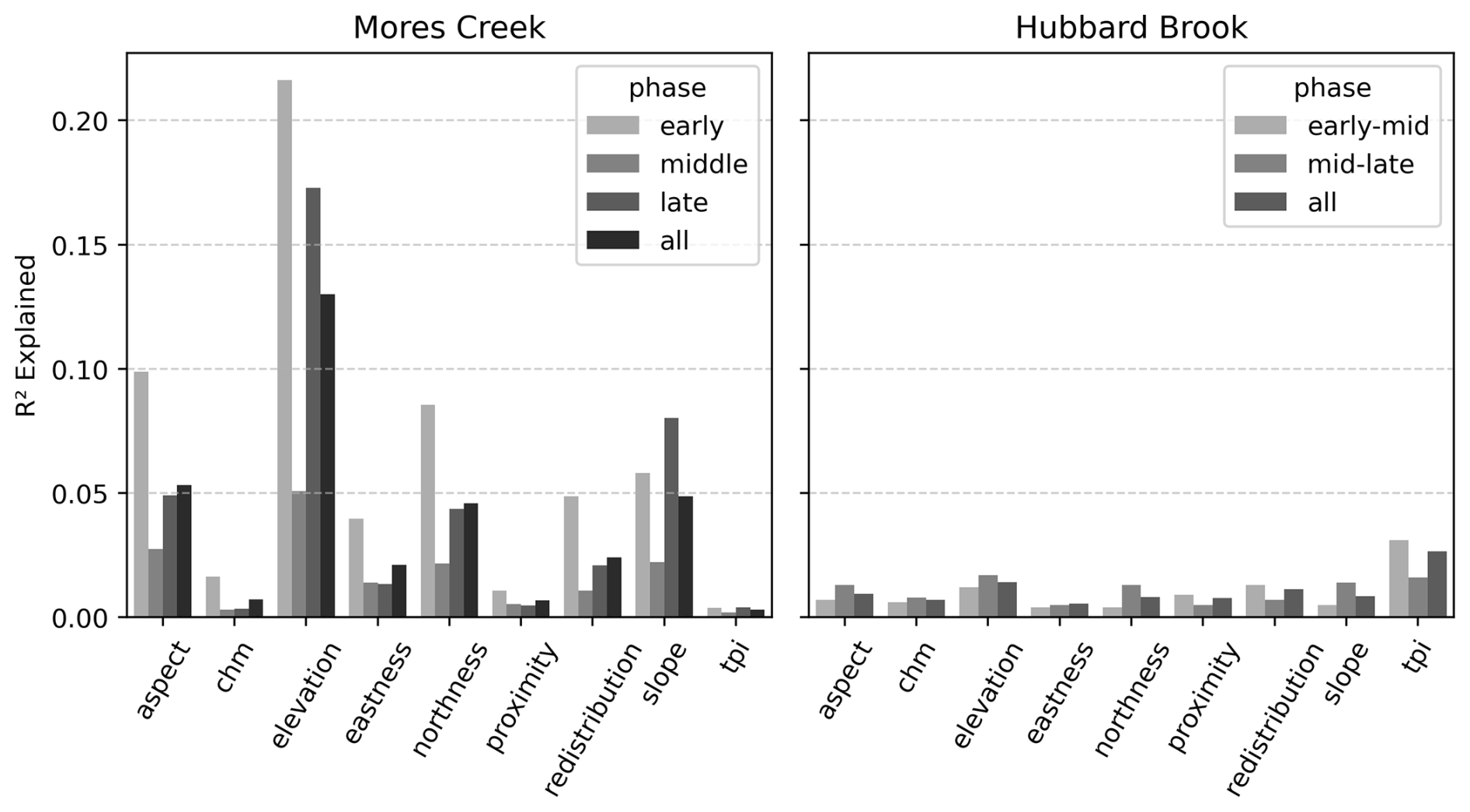
Figure 6 ANOVA analysis of explained variance in spatial RF modeled snow depth errors by select spatial predictors.

5.1.5 Terrain influence on model error across seasonal phases

The relationship of land cover and terrain metrics to the model residuals was further assessed at each study site using ANOVA statistical tests (Fig. 6). At Mores Creek, ANOVA revealed that explanatory power differed throughout the snow season and that several topographic and land cover predictors explained meaningful portions of the snow depth prediction error. Explanatory power was highest in the early season (total variance explained: 57 %), followed by the late season (39 %), the all-phase dataset (34 %), and lowest in the middle season (15 %), likely reflecting the more stable and predictable snowpack conditions during mid-winter. In the early season, aspect and northness, redistribution index, and elevation were the top predictors of model errors, each achieving high R² values relative to other phases and collectively accounting for a large share of the explained variance. Elevation effects persisted across all phases, though their relative importance decreased in the middle season before increasing again in late season, suggesting that snow depth error patterns are partly tied to elevation-dependent snow accumulation and melt timing. The late and all-phase datasets also showed aspect and redistribution as useful predictors of model error, though with reduced explanatory strength. In contrast, the middle season exhibited weaker terrain-driven patterns, suggesting that snow depth errors were less tied to landscape features during this period.

At the Hubbard Brook site, ANOVA revealed weak explanatory power of spatial predictors and the RF model residuals across all seasonal phases (early-mid: 9.1 %, mid-late: 9.8 %, all: 10.0 %), suggesting that errors are likely driven by predictive features omitted from the RF model. Of all features, TPI explained the highest variance in error overall (∼3 %). In the mid-late season slope, aspect, and northness showed slightly stronger relationships to the spatial error structure than in the early-mid season. For the early-mid season, TPI and the redistribution index were more closely related to the spatial error structure than later in the season. This suggests increased redistribution-driven errors earlier in the season (before 6 March) when snow is generally drier, colder, and more prone to redistribution.

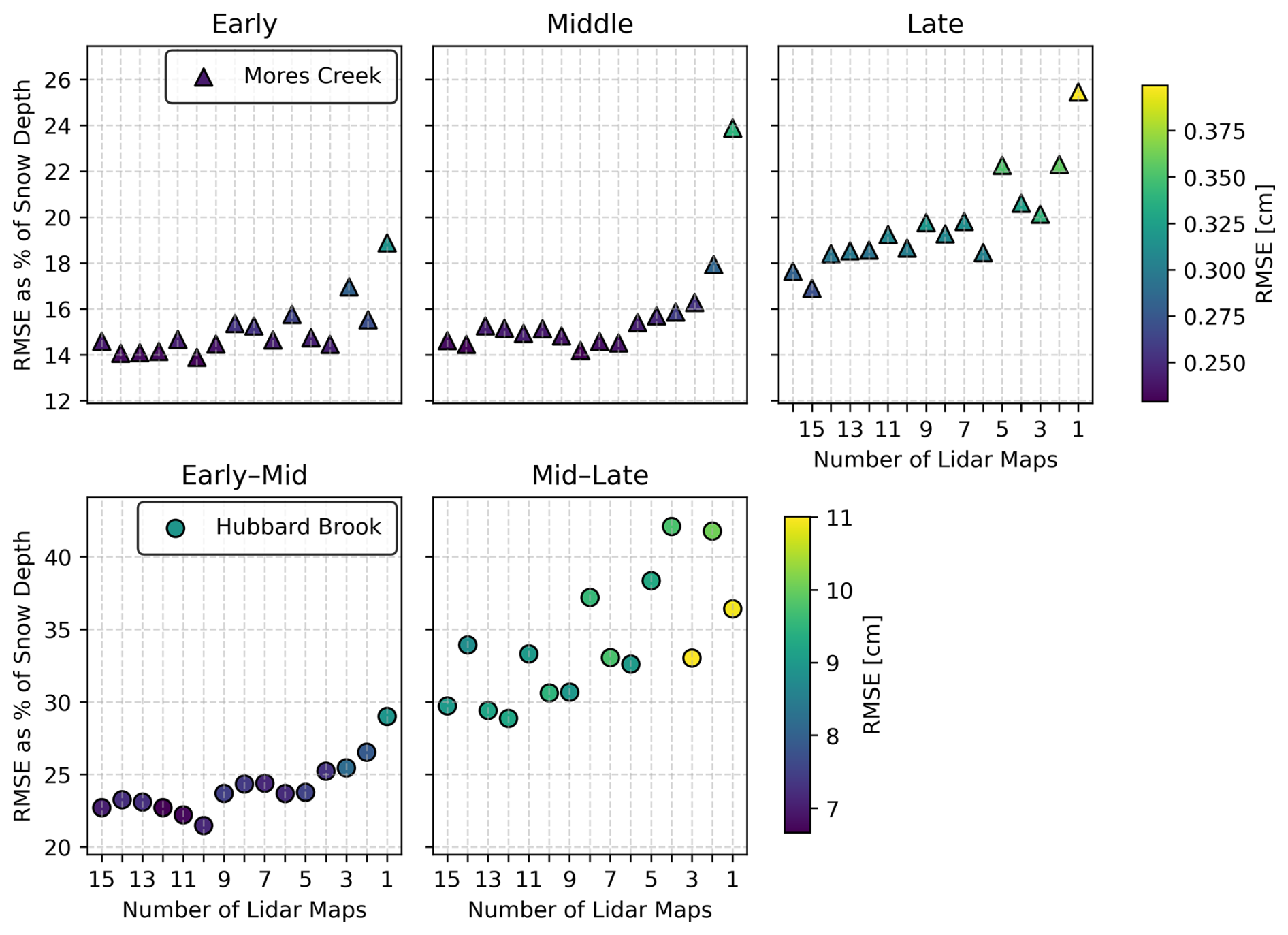
Figure 7 Drop analysis partitioned by seasonal phase for Mores Creek (top) and Hubbard Brook (bottom). For each iteration, the number of lidar maps indicates the number of maps used to train an RF model, which is then used to predict snow depths for a held-out random date. RMSE values are normalized by the average observed snow depths for the predicted date. One hundred iterations of each random drop scenario were performed, and markers represent the average of each error metric when predicting snow depths with the specified number of maps for a date in the specified seasonal phase.

5.2 Model performance across phases with varied data inputs

5.2.1 Sensitivity of model performance to Lidar acquisition frequency

Reduction in the number of lidar acquisitions increases errors in modeled snow depths, with impacts differing by snow accumulation phase (Fig. 7). For the Mores Creek, RMSE generally increased as fewer lidar acquisitions were used, with seasonal variations. Kendall's tau was positive and significant in all phases: early tau $=+\mathrm{0.62}$ (p<0.001), middle tau $=+\mathrm{0.53}$ (p<0.001), and late tau $=+\mathrm{0.80}$ (p<0.001), indicating reductions in RMSE with additional maps. Adding lidar dates (right to left) at the end of the season yields the largest decreases in RMSE, with early and mid-winter showing smaller but still generally monotonic model improvements. For Hubbard Brook, both phases also had positive and significant Kendall's tau values with +0.60 (p<0.001) for early-mid and +0.58 (p<0.001) for mid-late. The RMSE increases as the number of lidar maps decreases are more definitive in the mid-late period. Still, there is high variability across acquisitions, showing less clear relationships between increasing lidar acquisitions and performance during the mid-late seasonal phase. Examination of RMSE normalized as a percent of snow depth suggests that model error reductions may be more influenced by the range of observed variability (e.g., deeper late-season snow depths) than the model's predictive capacity.

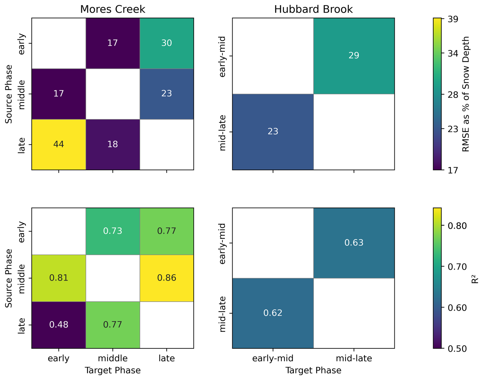
Figure 8 Cross-phase model performance heatmaps. Rows indicate the source phase used to train the RF; columns indicate the target phase used for prediction. Top row: RMSE expressed as a percent of observed snow depth (cell values annotated; shared colorbar at right). Bottom row: R² (annotated; shared colorbar at right). Left panels: Mores Creek. Right panels: Hubbard Brook. Metrics are means across iterations. Models were trained independently for each basin. See appendix for model statistics for each phase when trained on all data.

5.2.2 Cross phase model transferability

Cross-phase transfer analyses trained the RF model in one winter phase and tested it in another (Fig. 7). At Mores Creek, models trained on all phases perform best (RMSE 27–36 cm), and single-phase experiments show that mid-winter training generalizes well to late season (R² about 0.90, RMSE around 37 cm), while early-season training is a workable compromise for predicting both middle and late phases (R² about 0.75 in both phases, smaller RMSE in middle than late season). In contrast, models trained only on late-season data transfer poorly to earlier phases, indicating that late-season acquisitions alone are a weak basis for cross-season prediction. At Hubbard Brook, single-phase models show modest degradation relative to all-phase training (R² 0.81–0.83; RMSE 5–6 cm), and transfer between early–mid and mid–late phases is approximately symmetric (R² 0.62–0.63). Overall, these results indicate that mid-season acquisitions are the most transferable at Mores Creek, whereas at Hubbard Brook combining both accumulation and melt phases is more beneficial than optimizing for a single phase, likely because Hubbard Brook's transitional snowpack is more temporally variable.

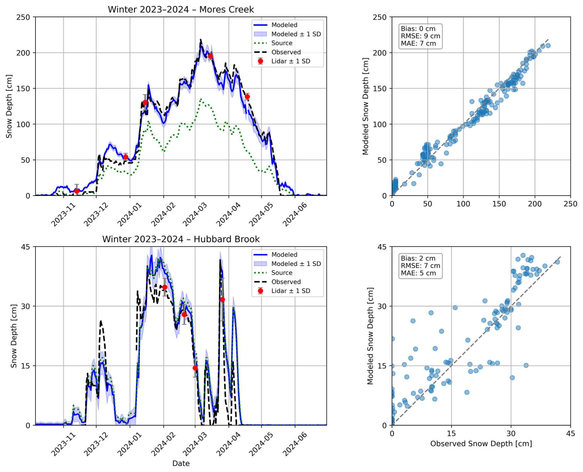
Figure 9 Point-scale time-series comparison between the ERA5-Land forced RF model (Modeled) and independent snow depth observations (Observed). Evaluation uses observations from the Mores Creek SNOTEL site (top) and the Hubbard Brook site 5 (bottom). Source refers to the source snow depth data used in the relative depth calculation for Mores Creek (ERA5-Land) and Hubbard Brook (ERA5-Land).

5.3 ERA5-Land and in-situ forcing comparison

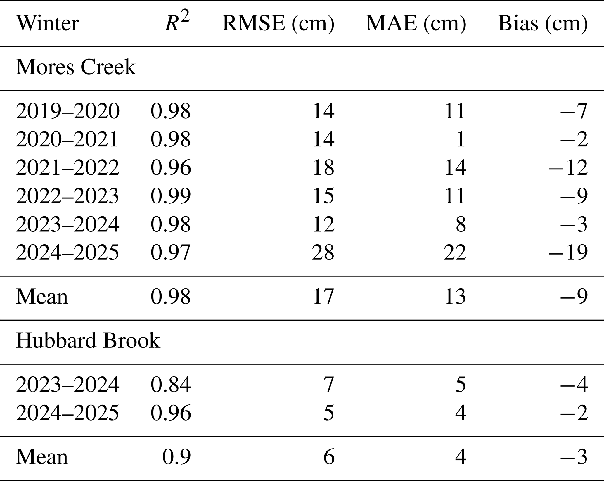
ERA5-Land was evaluated as an alternative to in-situ forcing, by repeating the RF training workflow using meteorological forcing variables from ERA5-Land. At Mores Creek, ERA5 forced predictions aligned closely with observations and with the in-situ forced model. Figure 9 shows the RF model is a considerable improvement over ERA5-Land's snow depth estimates. For the winter of 2023–2024 the ERA5-Land forced predictions were unbiased and closely matched station snow depth observations at the withheld SNOTEL site, with an RMSE of 9 cm and MAE 7 cm (Fig. 9). The example time series for the same winter shows that ERA5-Land forced and in-situ forced snow depths track together through accumulation and melt, with post storm increases and seasonal peaks coinciding. Coinciding mean lidar values on acquisition dates fall on (or between) the two curves, reinforcing the temporal fidelity (Fig. 10). Considering the full period between 2020–2025, ERA5- vs. in-situ–driven predictions over the same 10 000 pixels also showed high agreement in each individual winter season (mean R² of 0.98; range 0.96–0.99) with small differences (mean RMSE of 17 cm; range of 12–28 cm). Biases were consistently negative (mean −9 cm), indicating a slight ERA5-Land RF model underprediction relative to the in-situ model, with the largest departure in winter 2024–2025 (R² of 0.97; RMSE of 28 cm; bias of −19 cm). At Hubbard Brook, across both modeled winters (2023–2025), the ERA-Land forced snow depth predictions were similar to the in-situ forced model (mean R² of 0.90; range 0.84–0.96; RMSE below 7 cm; mean bias −3 cm). Performance across all nine in-situ sites was comparable between ERA5 and in-situ models (Table A3), if not slightly improved, using the ERA5 forced model (R² mean 0.83; range 0.59–0.95; RMSE mean 8 cm; range 6–10 cm; bias mean +3 cm; range −6 to 7 cm). Overall, ERA5-Land appears to be a reliable substitute where in-situ forcing data is unavailable.

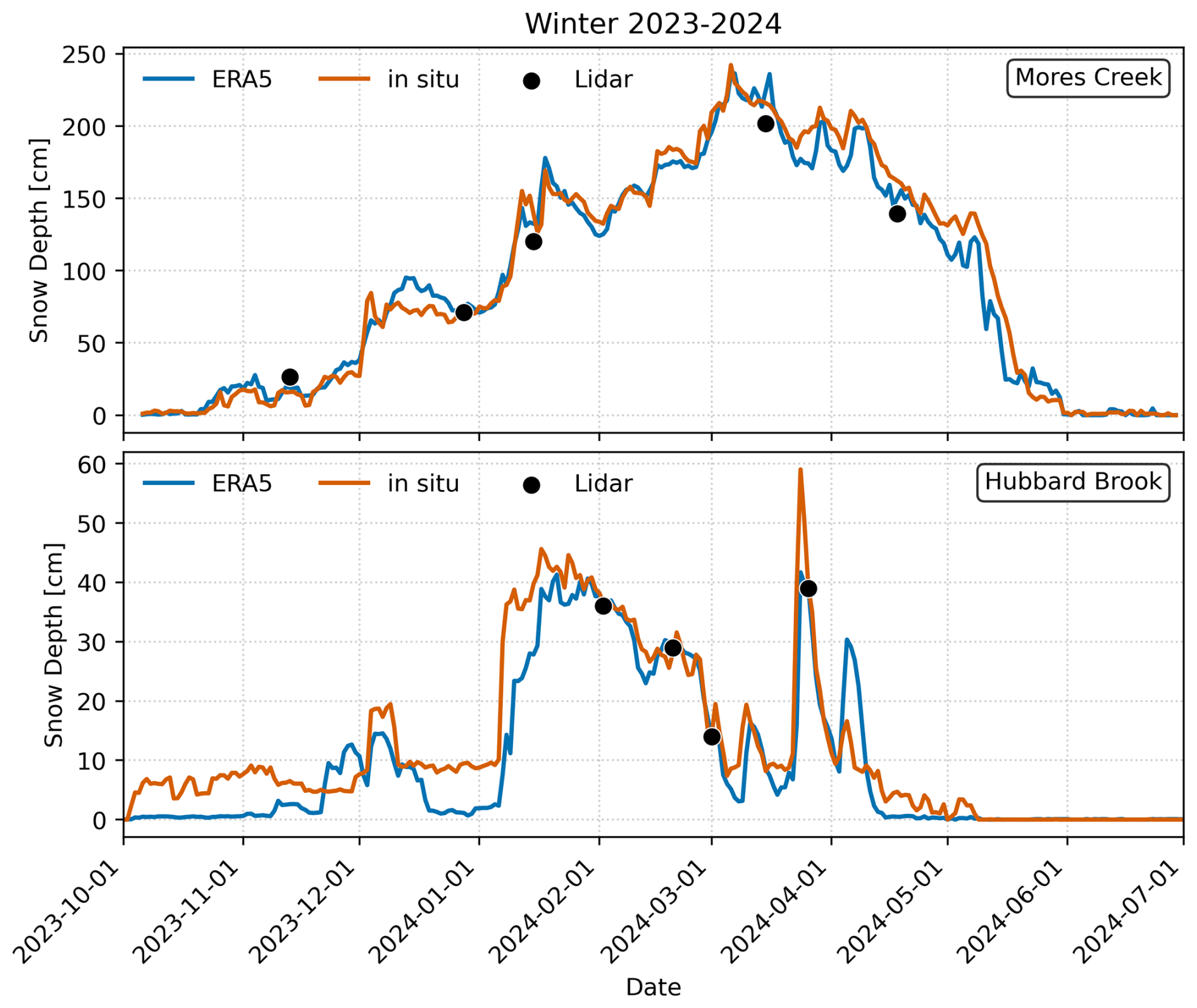
Figure 10 Basin average snow depth time series for RF models forced using ERA5-Land model reanalysis (ERA5) and in-situ meteorological data (in-situ) for winter 2023–2024 by study site. Basin average snow depths from lidar observations (Lidar) are also shown. Summary statistics for each year are included in Table A3.

6 Discussion

6.1 Effectiveness and limitations of RF for daily snow depth mapping

To generate spatially and temporally continuous snow depth estimates from sparse airborne lidar observations, we developed a machine learning workflow that reconstructs daily snow depth fields. We cast daily snow depth mapping as a relative-depth problem, training a RF on lidar-derived residuals (lidar – source time series) to encode the gridded residual map, while a daily driver (in-situ or ERA5-Land) provides temporal evolution. To keep learning within observed conditions, we enforce a valid-pixel/parameter-space mask and insert synthetic zero-depth maps at season start and end, which anchor accumulation and ablation and suppress spurious persistence between flights. Within these guardrails, RF functions as a robust non-parametric interpolator over high-dimensional static terrain/canopy features with modest influence from dynamic meteorological forcings, converting a handful of flights into temporally coherent daily snow depth maps without requiring a full energy-balance model (Liston and Elder, 2006; Marks et al., 1999). The workflow is portable, relying on a compact, reproducible feature set and versioned artifacts (masks, scalers), and can operate on ERA5-Land forcing where stations are absent. Across both basins, performance is promising, explaining about 90 % of the variance with RMSE of 8–28 cm (20 %–25 % of mean depth), MAE 5–19 cm, and near-zero bias. Despite the strong performance metrics, our approach is interpolative because RF performs well within the joint parameter space but degrades under distribution shifts (Reichstein et al., 2019; Yang et al., 2020), so we did not test for cross-basin transferability of a single RF model between Mores Creek and Hubbard Brook. In

Another limitation arises from the model's reliance on the temporal snow depth forcing from in-situ stations used as an input driver. Because the RF effectively predicts relative changes in snow depth through time, its accuracy depends on the fidelity of this forcing. If the forcing time series is biased relative to parts of a basin (e.g., biased low or returning to zero too early), then modelled pixels that historically retain deeper or more persistent snow may lose their dynamic characteristics or be forced toward zero values, despite physically retaining snow. This limitation underscores that the approach relies on representative, unbiased temporal snow depth inputs to capture the full spatial and temporal variability of the snowpack. Related work has shown that combining point snow depth with additional dynamic predictors and learned spatial patterns allowed the RF residual framework to maintain persistent snow at higher elevations even after a SNOTEL site had melted out, effectively extending the temporal utility of point measurements (Herbert et al., 2025).

6.2 Spatial errors and landscape features

Spatial patterns in RF residuals align closely with topography and canopy structure, and the strength of these controls varies by seasonal and regime. At Mores Creek, ANOVA indicates high explanatory power from terrain in the early season (57 % variance explained), moderate in late (39 %) and all-phase (34 %), and lowest in mid-winter (15 %), consistent with transition periods amplifying terrain-linked errors. The highest model residuals are co-located with wind redistribution features (e.g., cornices/lee zones) and aspect-driven insolation differences. Elevation, aspect/northness, TPI, and the redistribution index consistently emerge as the strongest landscape correlates of error. The SHAP analysis corroborates these relationships by ranking these predictors among the most influential for the RF estimates, with higher elevation and northness generally increasing predicted depth, and positive TPI (micro-ridges) and steep slopes suppressing it.

At Hubbard Brook, terrain explains a smaller share of residual variance overall (9 %–10 % across phases), reflecting the basin's smaller size and greater homogeneity. Model errors approaching 5 cm, around the limit of snow depth measurement uncertainty, suggest that much of the unexplained residual variance may be due to random error. Even so, microtopography (TPI), slope, and elevation lead both the ANOVA and SHAP diagnostics, mirroring map-scale residual patterns. Depressions (negative TPI) align with deeper conditions and reduced underbias, while micro-ridges (positive TPI) align with shallower conditions and overbias. High residual clusters along trails, streambeds, and within conifer patches suggest that local processes are not fully represented by current predictors (e.g., wind redistribution, compaction, canopy interception/unloading, cold-air drainage). Relative to static spatial terrain and vegetation features, dynamic forcings have smaller but seasonally meaningful SHAP contributions in both study basins (e.g., forward-looking temperature decreasing late-season depth; short lags in depth modestly increasing early-season estimates).

These diagnostics suggest that there is an opportunity for targeted refinements, including incorporating event-scale wind exposure (storm-wise upwind slope), radiation/shading metrics (clear-sky shortwave, horizon obstruction), canopy closure/density, trail/stream masks, and other remotely sensed variables to serve as wetness and compaction proxies for ablation. Because several terrain variables are correlated, SHAP magnitudes should be interpreted as directional influence and relative contribution rather than causal isolation; pairing SHAP with residual maps and ANOVA provides a more reliable picture of how landscape features structure model errors across seasons.

6.3 Considerations for Lidar cadence and seasonal timing of acquisitions

The drop-date experiments demonstrate a decrease in error as more flights are included, with clear diminishing returns after a small number of acquisitions. At Mores Creek, Kendall's tau is positive and significant across seasons, and the breakpoint behavior suggests that about five flights in early season, about four in mid-winter, and about five in late season recover most of the attainable skill. This aligns with findings from Herbert et al. (2025) in mountainous Colorado basins, which found diminishing improvements in RF model skill beyond four site-specific lidar surveys. Hubbard Brook exhibits the same qualitative pattern, though the errors' response to training surveys is more linear, which is consistent with its smaller, more homogeneous domain. Cross-phase tests indicate that models trained on the middle season transfer best to the late melt season; training using early season surveys can serve as a single-phase source for both middle and late seasons, but with larger errors for the late season. Training exclusively using late season surveys performs worst when predicting early season conditions. Although the ability to use late season acquisitions for early seasons predictions is not useful for snow forecasting, it provides value for reconstructing retrospective snow maps that can serve to validate moderate-resolution snow cover products (Gascoin et al., 2019; Stillinger et al., 2023). Similar performance of cross-phase models at Hubbard Brook may be due to the inclusion of observations near the seasonal peak in both seasonal phases (early-mid and mid-late).

Taken together, these results offer practical survey choices. If only one flight is possible, scheduling it during the middle season provides the best downstream performance for melt. With two flights, pairing early and middle offers broad seasonal coverage, whereas middle and late emphasizes melt accuracy. With three flights, early, middle, and late capture most of the gains at Mores Creek; in transitional basins like Hubbard Brook with milder temperatures and shallower snowpacks, fewer flights may suffice for basin-mean performance, while additional acquisitions primarily reduce local biases unless surveys are targeted to capture event-specific depth patterns (e.g., following large isolated snowfall events). Retaining the synthetic zero-depth anchors at the start and end of winter remains useful even as cadence increases; extra early or late flights mainly refine transition timing rather than mid-winter spatial structure. While we do not explicitly assess spatiotemporal snow depth prediction performance using the drop-date framework, future efforts could evaluate the coherence of daily snow depth products produced from a limited number of snow depth surveys. Collectively, these findings translate episodic lidar campaigns into daily, end-user ready products using a budget-aware cadence and seasonally informed timing.

6.4 Regime-dependent performance across western and eastern snowpacks

Model behavior differs systematically between the complex, wind-affected Mores Creek basin and the smaller, more homogeneous, forested Hubbard Brook watershed. At Mores Creek, large elevation and redistribution gradients create a strong spatial structure that the RF captures well, yielding clear gains over using a single in-situ site as a proxy for basin conditions; the biggest improvements occur in deep-snow zones where site-only approaches underpredict. At Hubbard Brook, basin-mean performance from the RF is similar to using the nearby reference site because the snow's spatial variability is smaller. Here, the model still reduces local biases in wind-sheltered areas and the basin upper elevations, where redistribution, compaction, and canopy effects deviate from the basin average. These contrasts are consistent with the diagnostics: terrain and redistribution metrics explain a larger share of residual variance at Mores Creek and have higher SHAP values, while microtopography dominates the modest landscape signal at Hubbard Brook. Although the two basins differ in spatial extent, each model was developed using the same sampling framework, scaled to basin size (50 000 samples at Mores Creek and 10 000 at Hubbard Brook). This consistent sampling approach minimizes the influence of domain size on model behavior, suggesting that observed differences primarily reflect contrasts in snowpack complexity and heterogeneity rather than sampling artifacts. Operationally, regime differences imply that larger heterogeneous western basins benefit most from adding lidar-informed residual maps, whereas in smaller transitional eastern basins, the primary value is correcting local departures from the mean and refining melt timing, with fewer flights often sufficient for acceptable basin-mean accuracy.

6.5 Monitoring strategies: targeted measurements, wall-to-wall mapping, and informed sampling

Recent work outlines a few strategies for expanding snow observations for water-supply forecasting: targeted measurements at locations with high predictive leverage (Raleigh et al., 2025) and wall-to-wall basin mapping from airborne (Geissler et al., 2023; Herbert et al., 2025; Painter et al., 2016) or proposed satellite observations (National Academies of Sciences, Engineering and Medicine, 2018). Each approach offers distinct advantages; for example, targeted monitoring is efficient and cost-effective, while wall-to-wall mapping provides complete spatial context.

Our results suggest a complementary third path of informed sampling. Because the relative-depth RF learns a per-pixel snow depth map from a limited number of flights and propagates daily evolution from a single driver, future campaigns may not need to be strictly wall-to-wall. Flight lines can instead be designed to cover the landscape units that concentrate model skill and error (e.g., elevation and aspect bands, wind-redistribution zones, canopy classes) identified by our residual and SHAP analyses, and scheduled according to the cadence results. This informed design preserves daily mapping capability while reducing cost and latency, bridging elements of targeted measurements and wall-to-wall approaches to support operational snow monitoring. As a future direction, we propose testing selected, information-rich flight lines focused on these key landscape units to evaluate how well they preserve daily mapping performance while improving efficiency.

6.6 Portability, data requirements, and path to operations

The workflow is portable because it depends on a compact set of inputs that are common to many basins: a snow-off baseline to derive static terrain and canopy layers; a handful of snow-on lidar maps to learn a per-pixel adjustment map; a single daily driver time series (from a local station where available or ERA5-Land where it is not); and a valid-pixel mask with synthetic zero-depth anchors at the seasonal endpoints. These components produce versioned artifacts like masks, scalers, and trained models, that can be transferred and retrained in new basins with modest effort. In data-sparse settings, ERA5-driven operation is feasible; the results here indicate that a reanalysis time series can supply the temporal evolution while lidar defines the spatial adjustment, enabling daily mapping where in-situ networks are limited.

Operational use benefits from a few safeguards. Because the method is intentionally interpolative, predictions should be limited to the observed parameter space and accompanied by routine checks for distribution shift and representativeness of the dynamic snow depth forcing. When a shift caused by, new storm types, unusual warmth, or evolving canopy, additional flights can be scheduled during the phases shown to add the most value, using the cadence results to target timing. Uncertainty should be reported alongside depth maps, using techniques that rank the overall accuracy agreement (Kim et al., 2017; Pan et al., 2025), so that managers see both expected conditions and plausible ranges. Finally, when depth must be translated to SWE for allocation decisions, the added uncertainty from density assumptions should be made explicit. With these practices, the approach provides a practical route from episodic airborne surveys to daily, basin-scale products that support melt-season operations, road and access planning, and short-term water management.

7 Conclusions

This study shows that a relative-depth RF model can use a small number of airborne lidar acquisitions and a single daily snow depth driver to produce temporally coherent, basin-scale daily snow depth maps in contrasting snow regimes. The model learns lidar–driver residual patterns on flight days and applies them between flights, yielding accurate, meter-scale fields without a full energy-balance model, provided predictions remain within the observed parameter space. Across both basins, the approach explains roughly 90 % of the variance with typical errors of about 8–28 cm and near-zero bias, demonstrating that episodic lidar surveys can be leveraged for daily mapping with modest data requirements.

Spatial diagnostics and feature attributions confirm that terrain and land cover organize both predictions and errors in a regime-dependent way. Elevation, aspect/northness, microtopography, and redistribution proxies exert the strongest influence, with signals most pronounced during transitional periods. In the heterogeneous, wind-affected Mores Creek basin, the model provides substantial gains over using an in-situ site alone, particularly in deep-snow zones, whereas in the smaller, more homogeneous Hubbard Brook basin, the main benefits are reducing local biases and refining melt timing rather than dramatically improving basin-mean metrics.

Cadence and forcing experiments translate directly into survey and driver design. Errors decline as additional lidar flights are added, with clear diminishing returns after only a few acquisitions: at Mores Creek, roughly five early-season flights, four mid-winter flights, and five late-season flights recover most of the attainable skill, while at Hubbard Brook a smaller number of surveys (three early–mid and five mid–late flights) is sufficient for similar basin-mean performance. Where only one or two flights are feasible, prioritizing middle season acquisitions captures most of the attainable skill, whereas late-season-only training is least transferable. Using ERA5-Land as the temporal driver produces snow depth predictions that closely match those driven by in-situ measurements, with small, mostly modest biases, indicating that reanalysis forcing is a viable substitute in basins lacking station data. Together, these findings outline a practical path from episodic airborne lidar campaigns to cost-aware, daily snow depth products that can support melt-season operations, access and hazard planning, and short-term water management.

Appendix A

Table A1 Summary statistics for all snow-on lidar flights included in this study.

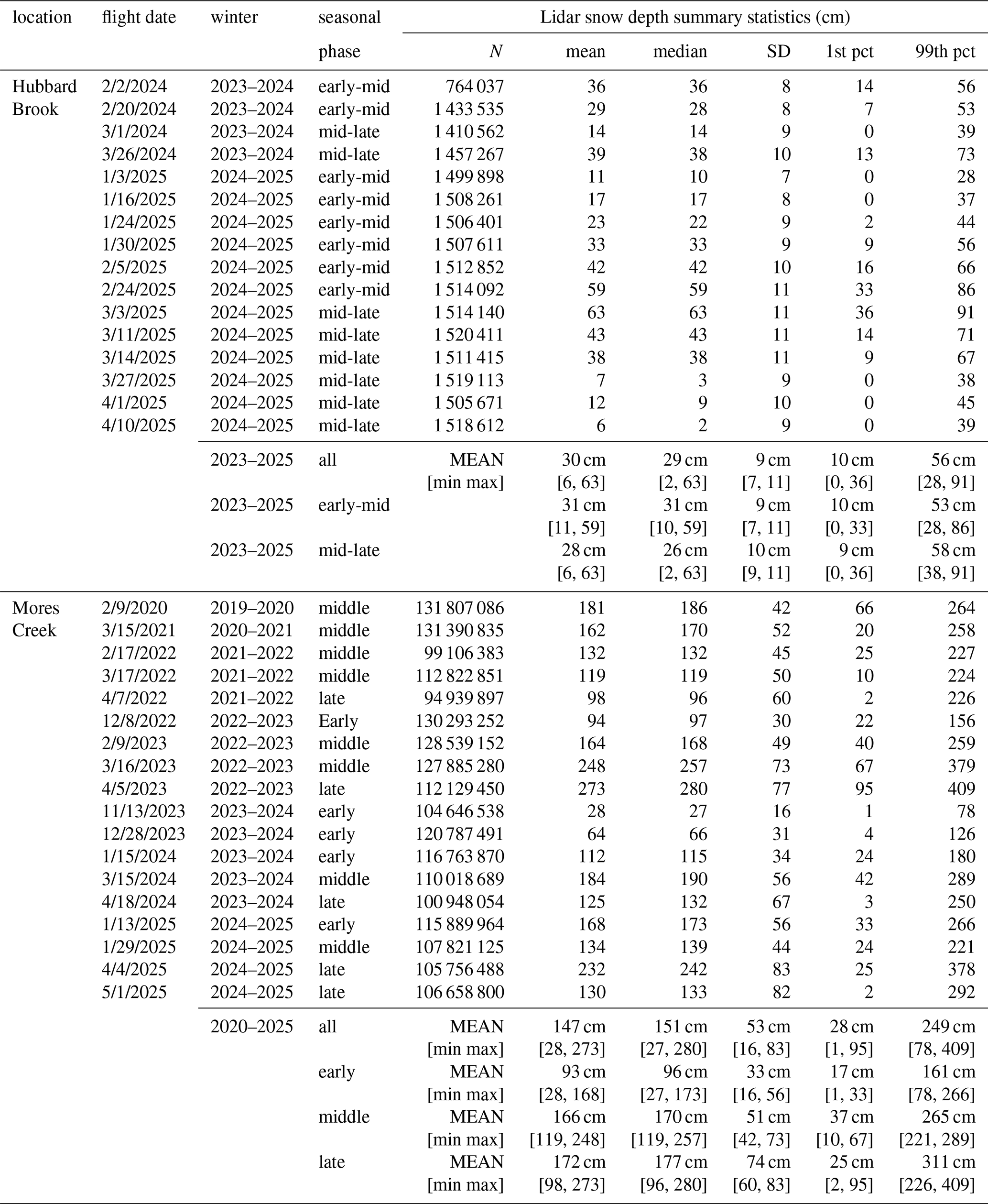
Table A2 Hyperparameters used in the RF models for Scikit-learn.

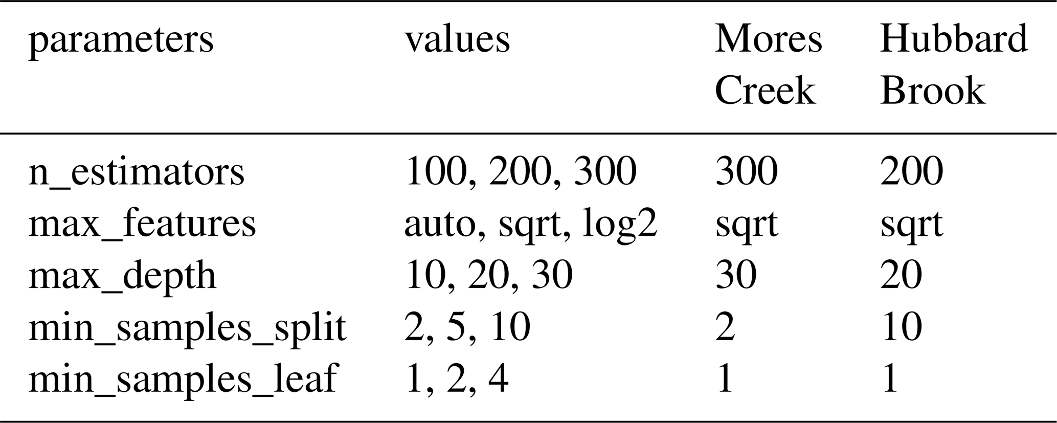
Table A3 Basin scale ERA5-Land driven RF model evaluation. This table compares the model-predicted mean basin snow depths when using a local in-situ site to ERA5-Land data to drive the model. Bias is calculated considering ERA5-Land model minus local in-situ model.