Machine learning for snow depth estimation over the European Alps, using Sentinel-1 observations, meteorological forcing data and process-based model simulations

Seasonal mountain snow is an indispensable resource, but accurate estimates of this water storage remain limited, even in the European Alps, where there is a dense network of in situ monitoring stations. In this study, we address Alpine snow depth estimation at a 100 m spatial resolution and sub-weekly temporal resolution over the 2015–2024 period using multiple input configurations within an extreme gradient boosting (XGBoost) machine learning (ML) model. We explore the potential of Sentinel-1 C-band dual-polarized synthetic aperture radar polarimetry (PolSAR) observations, and include either regionally downscaled meteorological forcing data or modeled snow depth as additional inputs to further explain interannual and spatial variability. A threefold nested cross-validation scheme is used to account for the spatio-temporal dependencies present in the snow depth data. XGBoost's internal booster and Shapley additive explanation (SHAP) values are used to relate the input features with the predictions for both dry and wet snow conditions. Our results indicate that the inclusion of PolSAR observations leads to modest improvements over a backscatter-intensity-based configuration, whereas the SHAP-based feature attribution reveals a high reliance of XGBoost on the polarimetric scattering angle and co-polarized (VV) backscatter intensity. Next, incorporating either meteorological forcing data or modeled snow depth substantially enhances predictive performance, particularly when spatially distributed training data, proven to be essential for capturing topographic controls on snow depth variability, are included. When supplemented with spatial training data and either meteorological forcing data or modeled snow depth estimates, XGBoost shows good agreement with nine snow surveys conducted in the Dischma valley (Switzerland), achieving correlation coefficients (R) of 0.76 and 0.78 and mean biases of 0.07 and 0.17 m, respectively. When applied to unseen locations across the Alps, the performance remains high, with R=0.80 and biases of −0.04 and −0.03 m, respectively.

1 Introduction

Globally, the spatial and temporal dynamics of seasonal snow have been changing over the last decades. Notarnicola (2022) and Bormann et al. (2018) report a negative trend in global annual snow cover, while Matiu et al. (2021) observed an overall decreasing trend in monthly mean snow depth (SD) for the months of November through May across the European Alps. These changes in seasonal snow dynamics have implications for society, ecosystems, and the climate system, given the critical role that snow plays in each of these domains. Snow namely serves as a natural water reservoir that contributes to river discharge, soil moisture and groundwater recharge (Gascoin et al., 2024; Dozier et al., 2016), and moreover fuels water basins used for hydropower generation (Bormann et al., 2018). Snow also provides drinking water to over 1.2 billion people worldwide, supports agricultural irrigation through snowmelt-driven runoff, and exerts substantial socioeconomic impacts, for example through traffic delays and accidents and by sustaining a multi-billion-dollar winter recreation industry (Bales et al., 2006; Barnett et al., 2005; Bormann et al., 2018; Qin et al., 2020; Sturm et al., 2017; Burakowski and Magnusson, 2012; Seeherman and Liu, 2015; Parthum and Christensen, 2022).

The climatic significance of snow is arguably even greater, albeit harder to monetize (Sturm et al., 2017). The combination of the high albedo of snow, which reflects a large portion of the incoming solar radiation, with the vast area of the world covered yearly by snow, enhances global cooling, and thus influences the Earth's surface energy balance (Warren, 1982; Groisman et al., 1994; Marks and Dozier, 1992). As a result of its importance, key snowpack properties such as SD and snow water equivalent (SWE), the latter relating to SD through snow bulk density, have been designated as essential climate variables (Gascoin et al., 2024; Global Climate Observing System, 2026), and various scientific institutions and international organizations have prioritized their enhanced observation and monitoring (Dozier et al., 2016; World Meteorological Organization, 2023).

To date, mountain SD and SWE have been observed and monitored using a wide range of measurement and modeling techniques, including manual and automated point measurements; airborne passive and active optical sensors; airborne and space-borne passive microwave radiometers; airborne and space-borne active microwave sensors, such as synthetic aperture radar (SAR); and process-based models. Manual and automated point measurements offer frequent data at many locations globally (e.g., Fontrodona-Bach et al., 2023, or Matiu et al., 2021), but fall short in capturing the snowpack’s spatial variability due to their relatively sparse and uneven spatial distribution within alpine regions (Miller et al., 2022; López-Moreno et al., 2015). Moreover, this type of monitoring is often conducted at relatively flat and open sites, rarely covers the highest elevations, and can disturb the snowpack (Dozier et al., 2016; Deems et al., 2013; Miller et al., 2022). Snow measurements derived from airborne passive and active optical sensors, such as photogrammetry-based SD maps (Bührle et al., 2023; Marty et al., 2019a) and lidar altimetry-derived SD and SWE products (Painter et al., 2016; Deems et al., 2013), provide high-resolution, spatially distributed measurements within mountain ranges, yet their use is constrained by limited spatial coverage and sparse temporal sampling (Tsang et al., 2022; Dozier et al., 2016; Hill et al., 2019). In contrast, space-borne passive microwave radiometers provide broad spatial coverage, but their effectiveness is reduced by a coarse spatial resolution (>25 km) and signal saturation in deep (≥0.8 m) snowpacks (Tedesco and Narvekar, 2010), limiting their applicability in mountainous regions. Alternatively, space-borne SAR has demonstrated potential for monitoring SD or SWE at finer spatial scales, particularly with Ku- and X-band observations (Tsang et al., 2022). Unfortunately, X-band observations are not publicly available, and no Ku-band satellite mission currently exists (Tsang et al., 2022), thereby constraining the development of such high-resolution SAR snow products over vast areas. Alternatively, multiple process-based snow models exist to estimate both SD and SWE at different spatial scales (e.g. Snowclim (Lute et al., 2022); SNOWPACK (Bartelt and Lehning, 2002); SnowModel (Liston and Elder, 2006a); factorial snowpack model (Essery, 2015)). Such models use meteorological forcings – often reanalysis data – to simulate the snowpack as one or multiple layers; solving mass and energy balance equations and mathematically representing the physical processes occurring within the snowpack. However, due to uncertainties in the forcing data and/or limitations in model representation, the modeled snow properties may differ substantially compared to in situ measurements and among each other (e.g., Terzago et al., 2020, Largeron et al., 2020, and Ryken et al., 2020).

Recently, SD retrieval algorithms have been developed that utilize Sentinel-1 (S1) active microwave observations at C-band (∼5.4 GHz). For instance, Lievens et al. (2022) use C-band co- (VV) and cross- (VH) polarized backscatter intensity observations in a conceptual change detection algorithm, which allows them to estimate SD across the European Alps at sub-kilometer spatial resolution. This algorithm was developed based on the results of Lievens et al. (2019) and Brangers et al. (2024b), who demonstrated the sensitivity of active microwave observations to snow at C-band. These previous studies have focused on C-band backscatter intensity in co- and cross-polarization, demonstrating that under dry snow conditions, an increasing snowpack depth leads to enhanced signal depolarization. This depolarization is thought to be related to snow volume scattering, (multiple) scattering on anisotropic snow crystals or clusters of crystals, and scattering at snow (or snow-ground) layer interfaces. As a result, mainly VH, or the ratio of VH to VV backscatter intensity is sensitive to an increasing SD (Lievens et al., 2019; Tsang et al., 2022). Jans et al. (2025) further explored the sensitivity of S1 C-band backscatter intensity observations to seasonal patterns of SD and SWE across the European Alps. In addition, Jans et al. (2025) emphasize the potential of S1 C-band dual-polarized SAR polarimetry (PolSAR) for SD retrieval, through the use of derived PolSAR variables that inform about the dominant snow scattering mechanism (i.e., a polarimetric scattering angle that increases with a growing snowpack), or about the intensity of the total received backscatter (i.e., the first Stokes parameter). Previous work has explored PolSAR for wet snow or snow cover area detection (Tsai et al., 2019; Varade et al., 2020), but no operational retrieval algorithms currently exist that utilize dual-polarized PolSAR observations for estimating mountain SD or SWE.

Despite its ability to characterize mountain SD at high-resolution over vast areas, the algorithm of Lievens et al. (2022) shows limited performance during periods of wet and shallow snow, in forested areas, or after frequent freeze-thaw events (Lievens et al., 2022; Brangers et al., 2024b). To address some of these limitations, Dunmire et al. (2024) implemented machine learning (ML) to enhance S1-based SD estimates at a high spatial resolution (100 m). They utilized an extreme gradient boosting model (XGBoost; Chen and Guestrin, 2016), incorporating input features related to topography, land and snow cover, and S1 C-band backscatter intensity. For the latter, they focused on the same satellite observations used by Lievens et al. (2022), namely VV backscatter intensity, and the cross-polarization ratio, defined as the ratio of VH to VV backscatter intensity. Other studies have similarly explored the application of ML for estimating SD and SWE, both with and without integrating S1 C-band satellite observations (Xiong et al., 2022; Daudt et al., 2023; Broxton et al., 2024; Duan et al., 2024). Similarly, multiple authors have explored the potential of ML in a hybrid physical/data-driven approach to enhance the outcomes of snow models (e.g., Wang and Tian, 2024; Pomarol Moya et al., 2026). Thereby, additional information relevant to the snowpack can be incorporated, such as S1 C-band observations. A similar approach has been used by Brangers et al. (2024a), De Lannoy et al. (2024) and Dunmire et al. (2026) within a data-assimilation setup, which used S1 C-band snow retrievals to enhance modeled SD. Additionally, ML models can also be used as emulators, replacing physical models by directly estimating SD from meteorological forcings (e.g., Charbonneau et al., 2025). Nevertheless, few studies have investigated ML setups that directly integrate modeled SD with S1 C-band observations. Moreover, direct comparisons between SD ML configurations incorporating modeled SD and those using meteorological forcing data as emulator remain scarce, leaving unresolved whether meteorology-driven ML setups can achieve performance comparable to configurations that explicitly include modeled SD.

In this manuscript, we further investigate the potential of ML with different input configurations to accurately estimate SD across the European Alps, essential for accurately quantifying the annual water stored as snow. To this end, we first conduct various experiments comparing the performance of S1 C-band backscatter intensity with PolSAR observations to quantify the added value of PolSAR observations relative to, and in combination with, backscatter intensity. To gain insights in when and where which type of satellite observations contribute to the SD predictions, we use feature importance (FI) analysis under both dry and wet snow conditions. We further evaluate the added value of incorporating meteorological forcing data and process-based snow model SD estimates as features in the ML model, to assess improvements in capturing interannual and site-specific variability, and to determine whether S1 observations remain influential. To validate our approach, we implement a threefold nested cross-validation (nested CV) framework, which masks subsets of the data during training and predicting (testing). This framework accounts for the spatial, temporal and spatio-temporal dependencies in the data, an essential consideration when validating ML models for spatio-temporal purposes (Meyer et al., 2018). Finally, to address the limitations of relying solely on point-based training data for spatial prediction and representing topographic effects on the estimates, we compare models trained with and without airborne snow survey data, and validate predictions against nine airborne photogrammetry surveys in the Dischma Valley, Switzerland.

2 Data

Various datasets were collected and reprojected (and/or resampled) to two geographic grids used in this study: the ∼100 m ($\mathrm{1}/\mathrm{1008}$°) resolution World Geodetic System 1984 (100 m WGS84) grid, used for fine-resolution datasets or to preserve more details in the target (SD) and auxiliary datasets, and the ∼500 m ($\mathrm{5}/\mathrm{1008}$°) WGS84 grid (500 m WGS84), used for the coarse-scale and satellite datasets. Table 1 provides an overview of the data products and the grid to which each was aligned to be used within this study.

Table 1 Overview of the datasets and their associated targeted resolution. The 100 and 500 m resolutions refer to the spatial resolution of the WGS84 grid.

2.1 In situ SD measurements

We compiled in situ SD data over the European Alps by combining stationary and point-based measurements with airborne photogrammetry snow surveys, sourced from multiple regional providers across the Alpine countries (Fig. 1). Point-based measurements were collected for the time period 2015–2024, and include data from Austria (provided by Geosphere Austria, formerly ZAMG), France (from measurement stations operated by partners under agreement of MetéoFrance), Italy (collected in the autonomous regions of Valle d’Aosta, Trento and Alto-Adige, Piemonte, Lombardy and data provided by the International Center for Environmental Monitoring CIMA Research Foundation), and Switzerland (manual and automated point-based SD measurements collected and managed by the Swiss Federal Institute for Forest, Snow and Landscape Research (WSL) – Institute for Snow and Avalanche Research (SLF)). In addition, we augmented our SD dataset with measurement data sourced from the Synoptic Data platform and the National Oceanic and Atmospheric Administration's Global Historical Climatology Network-Daily database (GHCNd, Menne et al., 2012). With the addition of these data, our dataset also contained sites within Germany and Slovenia.

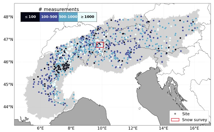
Figure 1 Spatial distribution of (dots) static or point-based measurement sites colored by the number of available data in time, and (red box) airborne photogrammetry snow surveys conducted across the Dischma valley, used to train XGBoost and evaluate the SD predictions. The light gray area delineates the Alpine region as defined by the Alpine Convention (Aureliano, 2020).

Next, we collected spatial SD measurements, derived from airborne photogrammetry (Marty et al., 2019a; Bührle et al., 2023) over the Dischma valley, Switzerland (Fig. 1, red box). A total of nine photogrammetry SD surveys (snow surveys) were added to our dataset, with an original resolution of 0.5 m (6 maps, measured yearly near peak SD between 2017 and 2022) or 2 m (3 maps, collected on 3 distinct days in 2016). For both resolutions, we applied a linear averaging and reprojected all surveys to the target grid of our SD estimates, the 100 m WGS84 grid.

2.2 S1 C-band PolSAR and backscatter intensity observations

Within our research, we collected data from the European Space Agency (ESA) and Copernicus S1A and -B satellites, which operate at C-band and share the same orbital plane with a 180° orbital phasing difference. Both have a 12 d repeat cycle. Combined, they offer a repeat cycle of 6 d over the study area. S1B, however, has been out of operation since 24 December 2021, and thus does not cover the complete study period (2015–2024).

S1 dual-polarized PolSAR observations were acquired from interferometric wide swath (IW) single look complex (SLC) data in dual-polarization (VV and VH) mode. The data were processed into two dual-polarized PolSAR variables: the polarimetric scattering angle (α) and the first Stokes parameter (S₀), using the Sentinel application platform (SNAP) toolbox, version 9, with processing steps described in Jans et al. (2025). These processing steps included applying precise orbit file corrections, radiometric calibration, debursting TOPSAR bursts, and merging sub-swaths into a single image. This was followed by the generation of the 2×2 covariance matrix (C2-matrix). The C2-matrix was then used as input for two distinct processing chains. The first one involved an eigenvector/value decomposition of the C2-matrix, followed by the H/α decomposition (Cloude and Pottier, 1997), from which α was derived. The second processing chain utilized the compact-polarimetry Stokes parameter generation to derive S₀ from the C2-matrix. Next, both variables were multilooked to ∼25 m to reduce speckle and finally, a Range Doppler terrain correction was applied to both variables, reducing (geometric) distortions due to topographical variations in the scene. For the latter, the Copernicus 30 m global digital elevation model (GLO-30 DEM) was used.

Next, co- (${\mathit{\gamma }}_{\text{VV}}^{\mathrm{0}}$) and cross- (${\mathit{\gamma }}_{\text{VH}}^{\mathrm{0}}$) polarized backscatter intensity variables were retrieved from ground range detected (GRD) amplitude data. Processing steps, described in Lievens et al. (2022) and Jans et al. (2025), were applied, including precise orbit file application, GRD border and thermal noise removal, radiometric calibration, terrain flattening to backscatter as γ⁰ (Small, 2011) and finally a Range Doppler terrain correction. As for the PolSAR variables, the Copernicus GLO-30 DEM was used during the processing steps. Additionally, local incidence angle (LIA) information was preserved and the cross-polarization ratio (${\mathit{\gamma }}_{\text{CR}}^{\mathrm{0}}$; calculated as the ratio between ${\mathit{\gamma }}_{\text{VH}}^{\mathrm{0}}$ and ${\mathit{\gamma }}_{\text{VV}}^{\mathrm{0}}$ in linear scale) was calculated.

Finally, both the PolSAR and backscatter intensity observations were rescaled and summer-corrected, to reduce inter-orbital and interannual start-of-season differences, respectively. To this end, we first reprojected the satellite observations onto the 100 m WGS84 grid using linear averaging, and resampled to the 500 m WGS84 grid by taking the mean. Then, we performed a first and second-order moment scaling (to correct for differences in the mean and variance) between orbits. Finally, from each scaled time series for each snow season (September–June), we subtracted the mean summer value (July–September) of the summer preceding that snow season, thereby reducing interannual start-of-season differences that are not related to snow conditions (e.g., changing vegetation). To indicate that these variables have been rescaled, we further append a superscript “s” (^s) to the satellite variable notation.

2.3 Snow cover data and wet snow mask

Snow cover data were obtained from two sources: binary snow cover information from the interactive multisensor snow and ice mapping system (IMS; U.S. National Ice Center, 2008) at 1 km resolution, and fractional snow cover (FSC) information from the moderate resolution imaging spectroradiometer (MODIS; Hall and Riggs, 2020a, b) at 500 m resolution. For the latter, we collected cloud gap-filled FSC data separately from the Terra and Aqua satellites, which we both reprojected onto the 500 m WGS84 grid using linear averaging. Subsequently, we combined the individual products using a weighted average, which accounted for the quality flags of each product, the time lag between the last cloud-free FSC observation and the current date, and the time lag of the individual satellite observations relative to each other (Appendix A). Next, a cutoff was set on the combined product, only allowing for FSC information less than 7 d before the current date. Finally, remaining gaps (3.95 % of the data points across the whole Alps and study period) were filled using IMS' binary snow cover information, reprojected to the same 500 m WGS84 grid using majority resampling. Hereby, a no-snow indication of IMS was set to an FSC value of 0 %, while an IMS snow covered pixel received a value of 100 %.

Additionally, a wet snow mask was acquired to differentiate between dry and wet snow periods. This dataset, based on S1 C-band satellite observations and obtained from the Copernicus Land Monitoring Service (CLMS) High Resolution Snow and Ice Monitoring (HRSIM) SAR Wet Snow in high mountains (SWS) product (Copernicus Land Monitoring Service, 2024), provides a binary classification between wet snow conditions, and dry, patchy or snow-free conditions. The data, available at 60 m resolution from September 2016 onward, were first reprojected onto the 100 m WGS84 grid using majority resampling, whereby the most frequently occurring SWS value within each 100 m target pixel was selected while excluding any no-data values. Subsequently, all non-wet pixels were classified as dry, while quality flags were retained to identify locations and periods with no (reliable) classification.

2.4 Meteorological forcing data

We downscaled 3-hourly meteorological forcing data over the European Alps to a 500 m spatial resolution, to serve as additional input to the ML model. To this end, we first collected coarse three-hourly meteorological forcing data with a 0.1° spatial resolution. Precipitation data were sourced from the multi-source weighted-ensemble precipitation (MSWEP, Beck et al., 2019) dataset, which combines various state-of-the-art reanalysis products with gauge and satellite observations (Beck et al., 2019). Other variables, including downward shortwave and longwave radiation, 2 m air temperature, wind speed, and 2 m relative humidity, were obtained from the multi-source weather (MSWX, Beck et al., 2022) product. This dataset is derived from coarse-scale European centre for medium-range weather forecasts reanalysis version 5 (ERA5) data refined through bias correction and downscaling using monthly 0.1° reference climatologies (Beck et al., 2022).

Subsequently, we applied bilinear interpolation in combination with different downscaling techniques, explained below, to account for local terrain features. To this end, the Copernicus GLO-30 DEM was employed, linearly averaged to the 500 m WGS84 grid to match the target resolution for the meteorological forcings. First, coarse-scale precipitation (P_coarse; [mm per 3 h]) was corrected as a function of elevation to account for orographic effects, using a rescaling function adapted from Huss et al. (2013), who corrected in situ precipitation data for gauge undercatch in a glacier mass-balance study. Thus, for each location x within the 500 m grid at time step t, $P_{{\text{coarse}}_{x,t}}$ was downscaled using the following equation:

$$\begin{array}{}\text{(1)}& {\displaystyle }\begin{array}{rl}{P}_{x,t}& =(\mathrm{1}-D)\cdot P_{{\text{coarse}}_{x,t}}\\ & +D\cdot P_{{\text{coarse}}_{x,t}}\cdot \left[\mathrm{0.75}+\mathrm{0.5}{\displaystyle \frac{z_x-z_{\text{min}}}{z_{\text{max}}-z_{\text{min}}}}\right]\\ & \text{ with }D={\displaystyle \frac{z_{\text{max}}-z_{\text{min}}}{D_{\text{dif}}}},\mathrm{0}\le D\le \mathrm{1}\end{array}\end{array}$$

with z_x the elevation [m] of the 500 m Copernicus GLO-30 DEM, z_min and z_max the minimum and maximum elevation [m] within an interpolation window – centered on the location x and spanning an area roughly matching the original 0.1° grid size – and D_dif a user defined difference in elevation, set to 250 m. The user defined difference was introduced to focus the corrections on the study area, with minor adjustments for areas with small elevation differences. Different from Huss et al. (2013), Eq. (1) limits the downscaled precipitation values between 75 % and 125 % of the original $P_{{\text{coarse}}_{x,t}}$ values.

The other forcings were adjusted as follows. The temperature was corrected using a seasonally varying lapse rate, following Liston and Elder (2006b), to account for elevation-dependent temperature variations. For relative humidity, we first converted to dewpoint temperature, then applied a lapse rate correction similar as for the temperature, and finally converted the corrected dewpoint temperature back to relative humidity (Liston and Elder, 2006b). Downward shortwave radiation was adjusted following the method of Fiddes and Gruber (2014), which involved partitioning the radiation data into direct and diffuse components, accounting for the elevation effect on the direct component, and applying a topographic correction to both components. In contrast, downward longwave radiation and wind speed were not adjusted after bilinear interpolation.

2.5 Process-based snow model Snowclim

Modeled SD estimates were obtained using Snowclim (Lute et al., 2022), a process-based enhanced single layer snow model utilizing a fully distributed energy and mass balance. We ran the model over the entire European Alps with the downscaled meteorological forcing data at a 500 m spatial and 3-hourly temporal resolution. To obtain daily values, the 3-hourly SD estimates were averaged to a daily time step. A description of the model's parameter settings, how they have been calibrated, and the model's performance when validated against in situ measurements, is provided in Appendix B.

2.6 Time-independent auxiliary data

In addition to time-dependent data, we employed time-independent auxiliary data, sourced from various providers. As with the other datasets (except the meteorological forcing and Snowclim data), these data were first projected onto the 100 m WGS84 grid, using linear averaging for continuous variables and majority resampling for categorical data. Forest cover fraction (FCF) data and land cover information, including a water mask, were acquired from the 2018 epoch of the 100 m Copernicus PROBA-V global land cover dataset (Buchhorn et al., 2020). Next, we used the Copernicus GLO-30 DEM to extract elevation and three topographic features: slope, aspect, and topographic position index (TPI), the latter quantifying the relative elevation of a grid cell concerning its surroundings within a predefined diameter. Slope and aspect were computed in MATLAB using the Geodetic (Craymer, 2022) and TopoToolbox (Schwanghart and Scherler, 2014) toolboxes, while TPI was calculated following the methodologies of Weiss (2001) and Lundblad et al. (2006). For this study, we computed the TPI using only the neighboring pixels of a specific grid cell, corresponding to a 3×3 grid window. Finally, we included a glacier mask, retrieved from the Randolph Glacier Inventory version 7.0 (RGI 7.0 Consortium, 2023), and collected the Sturm and Liston (2021) snow classes.

3 Methods

3.1 XGBoost model selection

Within this study, we deployed XGBoost to estimate SD across the European Alps. XGBoost is a tree-based traditional ML algorithm that constructs multiple decision trees in a sequential order, to minimize a differentiable loss function (Chen and Guestrin, 2016). Thereby, new trees are trained to fit the residual errors of the previously fitted trees, while incorporating regularization terms to reduce model complexity, and including additional mechanisms that contribute to its computational efficiency (Chen and Guestrin, 2016). We chose this ML algorithm after comparative experiments with other tree-based methods (including Random Forest, LightGBM and CatBoost) in which XGBoost showed the best performance and computational efficiency, as well as its use in recent snow studies (e.g., Dunmire et al., 2024, or Goodarzi et al., 2025).

3.2 Dataset preparation

We trained, validated, and tested XGBoost with various configurations on a dataset containing input features associated with each SD measurement (predictor variable) from the in situ measurement sites and snow surveys. To construct this dataset, we first excluded those stationary measurement sites located within glaciated areas, as well as those with less than 5 % non-zero SD observations. Subsequently, we identified the unique locations of the stationary sites within the 100 m WGS84 grid, and averaged time series from sites within the same grid cell. Furthermore, we excluded SD measurements during the summer months July and August, and resampled the data with a 500 m spatial resolution to the 100 m WGS84 grid using value replication.

The S1 data spatially and temporally coinciding with available SD measurements on the 100 m WGS84 grid include both ascending and descending orbits. This allows a single location to have two S1 observation values for the same SD measurement on a given date. Importantly, we chose not to exclude satellite observations with high or low LIA, as we assumed that XGBoost could effectively learn the relationships between these satellite observations and the corresponding SD. For each location and date with an available satellite observation, we also selected the corresponding (nearest) time-dependent non-satellite data and time-independent auxiliary data. This resulted in a dataset comprising 1022 measurement sites, with the distributions of observed SD and selected auxiliary variables shown in Fig. E1.

A similar procedure was applied for the photogrammetry snow survey data: for each SD measurement, the nearest input feature values within the 100 m WGS84 grid were selected and compiled into a dataset, linking each SD observation with its corresponding input features. Since satellite acquisitions did not always coincide with the exact date of the snow surveys, we used the most recent S1 observation prior to the survey, with a maximum offset of two days. Lastly, to represent the temporal component of our datasets, we computed the day of the year (DOY) for each instance. To account for the cyclic nature of the calendar year and prevent discontinuity between 31 December and 1 January, we transformed the DOY into two separate features using sine (DOY_sin) and cosine (DOY_cos) functions:

$$\begin{array}{}\text{(2)}& {\displaystyle }{\text{DOY}}_{\text{sin}}& {\displaystyle }=\text{sin}\left({\displaystyle \frac{\mathrm{2}\cdot \mathit{\pi }\cdot \text{DOY}}{n}}\right)\text{(3)}& {\displaystyle }{\text{DOY}}_{\text{cos}}& {\displaystyle }=\text{cos}\left({\displaystyle \frac{\mathrm{2}\cdot \mathit{\pi }\cdot \text{DOY}}{n}}\right)\end{array}$$

with n the number of days in the corresponding year.

3.3 Feature configurations and SD prediction

3.3.1 S1 PolSAR vs. backscatter intensity observations

To assess the performance of ML setups using S1 PolSAR versus backscatter intensity observations, XGBoost was trained and validated under three distinct configurations (Table 2), without including meteorological forcing data or Snowclim SD estimates in these experiments. For each configuration, XGBoost incorporated the same time-independent auxiliary features: elevation, slope, aspect, TPI, and FCF. Next, DOY features, FSC data and LIA information were included, the latter to indirectly account for orbital differences. The first configuration, referred to as PolSAR_ML, incorporated α^s and $S_{\mathrm{0}}^{\mathrm{s}}$ next to the shared common input features. The second configuration, focusing on backscatter intensity observations (Backscatter_ML configuration), included ${\mathit{\gamma }}_{\text{VV}}^{\text{0,s}}$ and ${\mathit{\gamma }}_{\text{CR}}^{\text{0,s}}$ as satellite input features. In addition, we combined the PolSAR and backscatter intensity satellite input features (Combination_ML configuration), to identify the satellite variables most effectively used within XGBoost.

Table 2 Features included in the ML configurations tested in this study: polarimetric scattering angle (α^s); first Stokes parameter ($S_{\mathrm{0}}^{\mathrm{s}}$); cross-polarization ratio (${\mathit{\gamma }}_{\text{CR}}^{\text{0,s}}$); co-polarized backscatter intensity (${\mathit{\gamma }}_{\text{VV}}^{\text{0,s}}$); cumulative snow precipitation and wind speed (P_s,c and Ua_c, summed between 1 September of the corresponding snow year and the prediction date); cumulative shortwave radiation and melt days over the preceding 7 d (SWd₇ and MD₇); mean daily temperature on the prediction day (T_a); and Snowclim SD estimates (SD_SC). A cross (×) denotes the presence of a feature in a given configuration. Additionally, all configurations include the following input features, indicated as common in the table: elevation, slope, aspect, topographic position index (TPI), forest cover fraction (FCF), fractional snow cover (FSC), sine and cosine values of the day of year (DOY_sin and DOY_cos), and the local incidence angle (LIA).

3.3.2 S1 observations plus meteorological forcing data or Snowclim SD estimates

The satellite observations were further complemented with either meteorological forcing data (Weather_ML configuration) or Snowclim SD estimates (Snowclim_ML configuration) to better resolve interannual and in-between-site variability (Table 2). The Weather_ML configuration was an extension of the Combination_ML setup, now including cumulative snowfall, cumulative wind speed, cumulative shortwave radiation, a cumulative number of melt days, and the mean daily temperature (T_a). Cumulative snowfall (P_s,c) was estimated by first calculating the daily fraction of precipitation falling as snow, based on temperature, precipitation and relative humidity using the bivariate logistic regression model described by Jennings et al. (2018), and subsequently summing these fractions from 1 September of the corresponding snow year up to the prediction date. Similarly, the cumulative wind speed (Ua_c) was derived as the sum of the daily wind speed from 1 September of the corresponding snow year up to the prediction date. Cumulative shortwave radiation (SWd₇), on the other hand, was summed over the seven days preceding the prediction date. Similarly, the cumulative number of melt days (MD₇) was defined as the number of days with a maximum temperature above 0 °C within the 7 d preceding the prediction date. The Snowclim_ML configuration did not include meteorological forcing data as direct inputs, but instead makes use of modeled SD estimates from Snowclim (SD_SC), which are driven by meteorological conditions.

3.3.3 XGBoost SD prediction procedure

Prior to being used in XGBoost for SD prediction, each feature was standardized individually, using the mean and standard deviation calculated from the training set values. This standardization was consistently applied to the validation and predicting (test) datasets as well, ensuring compatibility across all data splits. Since S1 observations are influenced by orbit-specific viewing geometries – potentially resulting in different SD estimates – input features from ascending and descending orbits were fed to XGBoost separately. In case a location had both an ascending and descending satellite observation on a given date, the mean of both XGBoost SD outputs was taken.

3.4 Spatio-temporal nested cross-validation and hyperparameter tuning

The concept of nested cross-validation (nested CV) has been extensively utilized in other studies (Dora et al., 2018; Abdulaal et al., 2018; Parvandeh et al., 2020), as it enables a correct characterization of the generalization error of an ML model (Blancas, 2021). Figure 2 illustrates that nested CV involves both inner and outer resampling to, respectively, train and tune the ML model (and its hyperparameters), and evaluate predictions on unseen and independent test data. Considering the susceptibility of SD measurements to spatial and temporal autocorrelation, we implemented the CV strategy described in Landschoot et al. (2012) within a threefold nested CV framework for the site data (excluding the snow surveys), in which subsets of the data are masked during training, validation and predicting (testing). To this end, the data of the site measurements were partitioned into spatial, temporal and spatio-temporal folds.

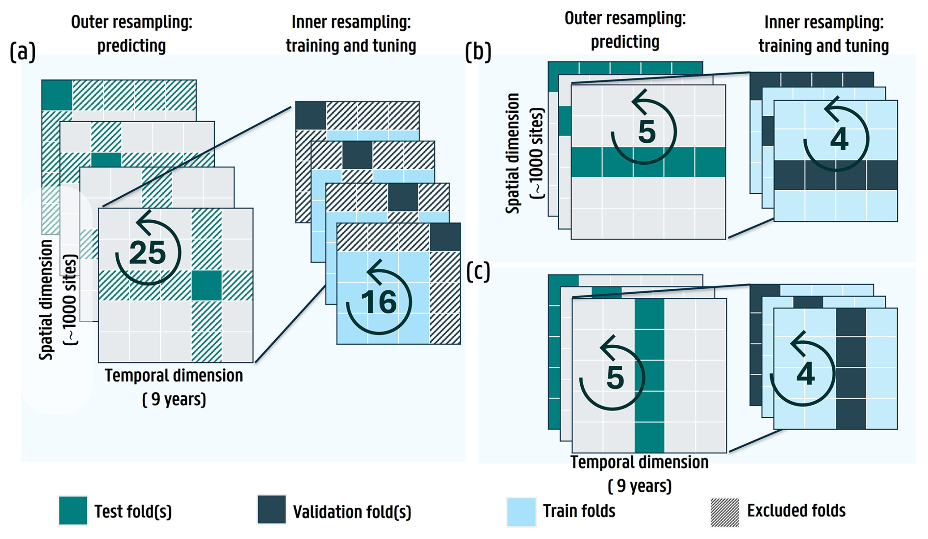
Figure 2 Principle of nested CV for (a) the spatio-temporal setup, (b) the spatial setup and (c) the temporal setup. The predicting (test) and training folds during outer resampling are colored in turquoise and light gray respectively. The validation and training folds during inner resampling are colored in dark and light blue. The striped boxes in (a) represent the excluded folds during training and testing within the spatio-temporal setup. During outer resampling, predictions are made with the trained ML model, with hyperparameters that are tuned during inner resampling. The numbers indicated in the arrows represent the amount of times outer and inner resampling are performed, respectively. For (a), four iterations are shown, while for (b) and (c), three iterations are displayed.

The spatial folds were constructed using a two-step approach: first, sites located within five km of one another were grouped into clusters, thereby preventing nearby sites with similar (climatic) characteristics and SD patterns from being split across training and test sets. Subsequently, these clusters were randomly assigned to five unique folds, ensuring that each fold contained a comparable amount of data and preserved a similar SD distribution. For the temporal folds, sites were not clustered; instead, all observations from a given snow season (September–June) and from across the study area were grouped into nine blocks (corresponding with the number of snow seasons for which SD data is available), which were then partitioned into five folds, again ensuring comparable fold sizes and a consistent SD distribution. Finally, by combining both fold-creation techniques, we constructed 25 unique spatio-temporal folds.

For each unique fold (five for spatial and temporal nested CV; 25 for spatio-temporal nested CV), we iteratively designated one fold as the test set during outer resampling, using the remaining folds for training and validation. To ensure independence of the test data, all data from the sites and/or years present in the test fold were excluded from the training and validation sets (Fig. 2).

The same approach was applied during inner resampling, to split the training and validation data used for tuning XGBoost's hyperparameters. To tune the hyperparameters, we utilized Scikit-learn's (Pedregosa et al., 2011) RandomizedSearchCV algorithm, employing the mean squared error (MSE) as loss function. A different random seed was set for each outer resampling loop, introducing variability in the selection of optimal hyperparameter combinations. During each loop, 150 hyperparameter combinations were chosen from a predefined tuning grid, based on the one provided in PyCaret (PyCaret, 2020). The hyperparameters yielding the best mean MSE score across the validation folds were selected. This approach produced independent predictions for every instance in the dataset, enabling the calculation of performance metrics and the construction of FI scores.

3.5 Feature importance scores

We used both XGBoost's booster and Shapley additive explanations (SHAP; Lundberg and Lee, 2017) values to assess the feature's impact on the SD estimates. For the booster, we selected the gain FI, which informs about the contribution of each input feature in minimizing the loss function during model training. As such, for every outer resampling loop within the nested CV framework, we computed the gain FI of the individual features during model training.

SHAP values, on the other hand, quantify the contribution of each input feature to an individual (SD) prediction, measured relative to an expected prediction (SD) value. Within the nested CV framework, SHAP values thus indicate how each feature influences the SD predictions made for the outer resampling predicting sets, relative to the average (SD) prediction computed from the training set. Consequently, SHAP values can be both positive and negative. To assess the overall global SHAP value FI during SD prediction, mean absolute SHAP values were computed for each input feature during every outer resampling loop. The latter were converted into relative contributions by normalizing them with the sum across all features.

We further used SHAP values to assess the contribution of the S1 PolSAR and backscatter intensity observations to the SD predictions throughout the seasonal evolution of the snowpack. To this end, for each site and snow season in the test sets, we first identified the periods during which a snowpack was present, based on the measured SD. The season start date was identified as the first date with SD≥10 cm, that was followed by nine consecutive days with SD≥1 cm. For low elevation sites with (very) shallow snowpacks, where this condition was not met for an entire snow season, the start of the snow season was marked by the first date with SD≥10 cm. Conversely, we defined the end of a site's snow season as the first day of a 10 d period with 0 cm SD, near the end of snowpack presence. In addition, we used the CLMS SWS product to distinguish, where possible, between dry and wet snow conditions. As this product is only available from September 2016 onward, the 2015–2016 snow season was omitted from the corresponding analyses.

3.6 Performance metrics

In addition to the FI and SHAP value analysis, several performance metrics were used to validate XGBoost SD predictions with measured SD. For each configuration and across all outer resampling predicting sets (thus the total dataset), we computed the spatio-temporal Pearson correlation coefficient (R), mean absolute error (MAE), root mean squared error (RMSE) and bias between predicted and measured SD (all averaged over time and space). Since cross-validation is conducted in both space and time, the performance metrics reflect the ML model’s ability to generalize across purely spatial, purely temporal, and combined spatio-temporal domains. Additionally, certain metrics were calculated on a per-site basis, such as the MAE.

Next, we evaluated XGBoost’s capability to generate spatial SD predictions by comparing them with the photogrammetry snow surveys conducted in the Dischma Valley, Switzerland. For this case, we trained XGBoost exclusively on stationary and point-based measurements, excluding spatial data from the snow surveys. Model training and hyperparameter tuning were performed using fivefold spatial CV, as this approach best reflects the intended application of the ML model: predicting SD on unseen locations across the European Alps within the time period of our S1 data collection. After training, XGBoost was applied to predict SD for each of the nine snow surveys, and performance metrics were computed.

We then repeated this process, but now incorporating all snow survey data except those of the targeted date into the training dataset. This resulted in nine independently trained and tuned XGBoost models, each applied to predict SD for the corresponding unseen snow survey. In this approach, we also employed spatial CV for training and tuning, where every training snow survey was randomly assigned to one of the five folds. This ensured that the distribution of training and validation data remained consistent across folds.

4 Results and discussion

4.1 Performance of ML configurations with S1 PolSAR and backscatter intensity variables

In general, all configurations (i.e., PolSAR_ML, Backscatter_ML and Combination_ML) achieve best results within the temporal nested CV framework (Table E1), and performance progressively deteriorates in the spatial and spatio-temporal frameworks (Table 3). This behavior is expected, as SD patterns within the same area (i.e., at the same sites) tend to recur across different years, such that SD prediction for an unseen snow season (i.e., the temporal framework) is inherently more favorable for XGBoost than prediction at unobserved locations (i.e., the spatial framework). Predicting at unobserved locations and during unseen snow seasons (i.e., the spatio-temporal framework), including times outside the study period is even more challenging, as XGBoost cannot exploit season-specific information from the training data nor rely on recurrent site-specific SD patterns. Consequently, because the intended application of XGBoost is to predict SD at previously unseen locations across the European Alps within the training dataset time period (e.g., Fig. 3a), reliance on the temporal framework would lead to an overly optimistic evaluation of model performance, whereas the spatio-temporal framework would provide a more conservative assessment.

Table 3 Overall performance metrics for the PolSAR_ML, Backscatter_ML and Combination_ML configurations for the spatial and spatio-temporal nested CV frameworks, when evaluated over all sites displayed in Fig. 1. The values inside the brackets denote the metric values when zero-measured SD are included in the evaluation.

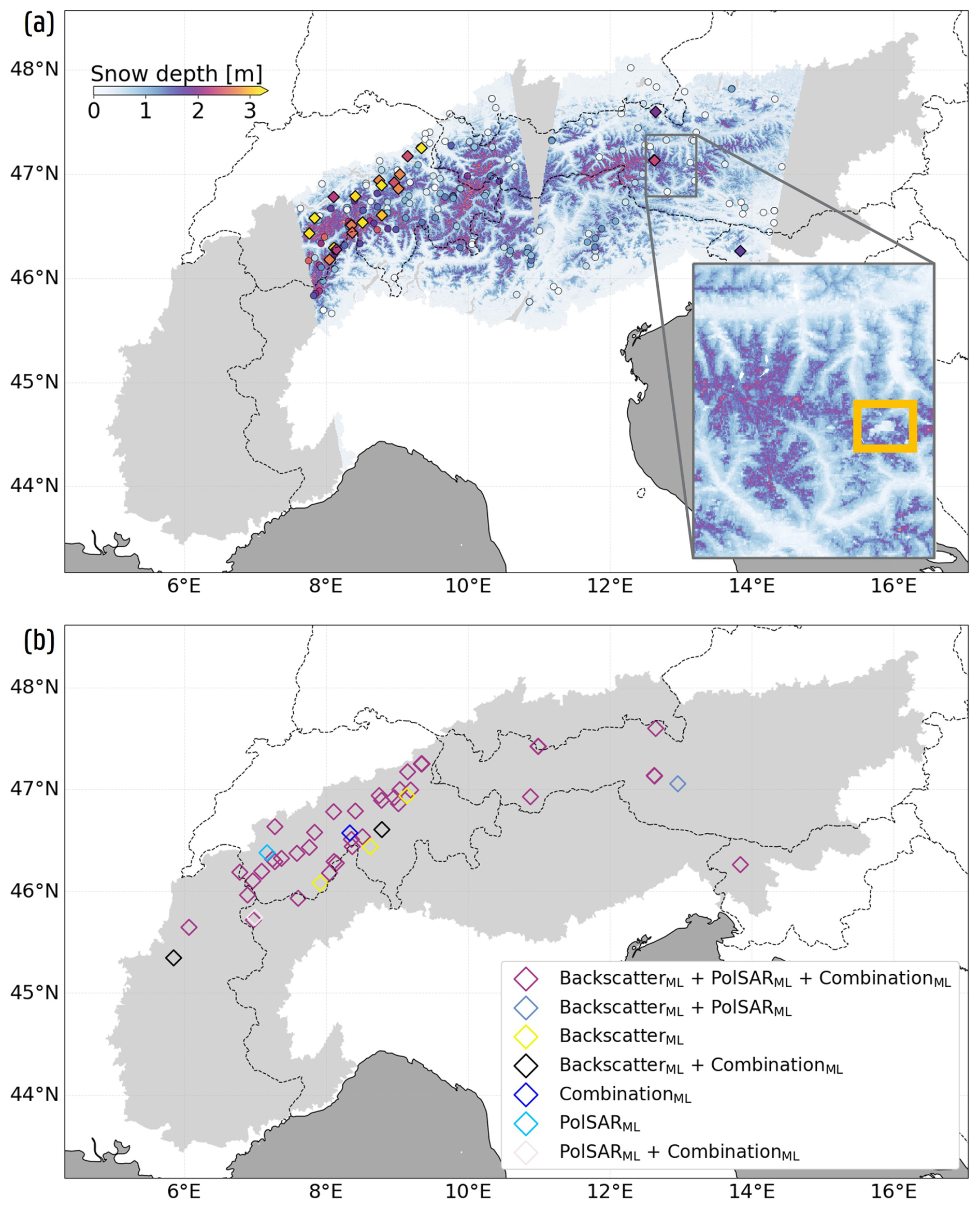
Figure 3 Spatial SD estimate and underestimation of the Combination_ML configuration. (a) Prediction on 18 January 2018 encompassing both an ascending and descending S1 observation, derived as the mean SD from the five XGBoost models trained within the spatial nested CV framework. Observations are indicated by dots and squares, with squares representing sites exhibiting a $\text{site-bias}\le -\mathrm{0.5}$ m for this framework (displayed in b). Estimates over Austria are highlighted to indicate an area of SD underestimation errors (yellow square) attributable to errors in the FSC input feature. (b) Measurement stations exhibiting a mean site $\text{bias}\le -\mathrm{0.5}$ m within the spatial nested CV framework (zero-measured SD excluded). Sites with fewer than 10 observations are excluded. Colors indicate the configurations for which this underestimation occurs. Across the displayed sites, 23 % of the observed SD measurements ≥2.5 m, compared to only 2 % across the full training dataset.

The absolute improvements of using PolSAR observations, as a replacement for (or in combination with) backscatter intensities, are small within all nested CV frameworks, or even minimal within some CV frameworks. Within the spatial framework, the PolSAR_ML and Backscatter_ML configurations display marginal differences in overall performance metrics (Table 3), which likely stems from the similar relationship of the variables with SD, and the spatial noise present in both types of S1 variables. The Combination_ML configuration also shows similar overall performance compared to the Backscatter_ML configuration, yet the improvements in MAE, computed per site, are significant (p≪0.05, 95 % confidence level), resulting in an overall MAE of 35 cm, a mean site-MAE of 29 cm, and a mean site-bias of −11 mm (excluding zero-measured SD). PolSAR observations moreover improve model performance for the spatio-temporal framework, with significant improvements in site-MAE for both the PolSAR_ML and Combination_ML configurations (p≪0.05, 95 % confidence interval). This improvement suggests that PolSAR observations, alone or in combination with backscatter intensities, more effectively capture the seasonal evolution of SD, a conclusion that is further supported by statistically significant gains in site-MAE (p≪0.05, 95 % confidence level) observed in the temporal nested CV framework. Nonetheless, also here the overall improvements remain limited, and the increased computational cost of processing S1 SLC data into PolSAR variables relative to deriving backscatter intensity from GRD data must be considered. Indeed, besides requiring separate processing chains to retrieve α and S₀ from the C2-matrix (Sect. 2.2), handling SLC data is more demanding, with raw images (∼5 Gb) substantially larger than GRD products (∼1 Gb).

Additionally, all three configurations exhibit difficulties in predicting high SD values at unobserved sites (Fig. 3), which likely arises from the scarcity of high SD observations in the training dataset (Fig. E1a). For the spatial nested CV framework, the PolSAR_ML, Backscatter_ML and Combination_ML configurations exhibit a bias of −1.46, −1.51 and −1.48 m for observed SD≥2.5 m, which further deteriorates in the spatio-temporal framework. This is also visible in Fig. 3a, when comparing the observations (squares) with the SD prediction, and in Fig. 3b, that displays sites with a $\text{bias}\le -\mathrm{0.5}$ m for the different configurations within the spatial nested CV framework (zero-measured SD excluded). Interestingly, many of the sites displayed in Fig. 3b also appear to have strong negative biases in Fig. 2a of Dunmire et al. (2024). Consequently, the reduced ability of XGBoost models, trained with S1 variables to explain interannual and site-specific variability, to predict high SD values must be taken into account when deploying the model across the European Alps, particularly when applying it beyond the temporal range covered by the training data.

4.2 Feature importance for ML configurations with S1 PolSAR and backscatter intensity variables

Across the configurations and nested CV frameworks, FSC and elevation consistently emerge as the most important features, similar to what has been reported by Dunmire et al. (2024), indicated by both XGBoost’s internal gain metric and SHAP values (Fig. 4a and b). FSC is particularly important, which makes the predictions prone to potential errors in this input feature (e.g., the high-alpine area in the yellow box in Fig. 3a, where erroneously low FSC-values led to SD underestimation). The gain FI (Fig. 4a) moreover indicates an increasing FSC importance when transitioning from temporal to spatio-temporal nested CV frameworks (∼25 % to >40 %), with an opposite trend for elevation (∼20 % to ∼10 %). When predicting at unseen locations, XGBoost seems to rely more heavily on FSC to distinguish snow-covered periods, and cannot rely as much on recurring SD patterns that display a strong relationship with elevation. Finally, the DOY features, which help capturing the seasonal variations in the estimates, also emerge as important inputs, as reflected across the configurations in both Fig. 4a and b.

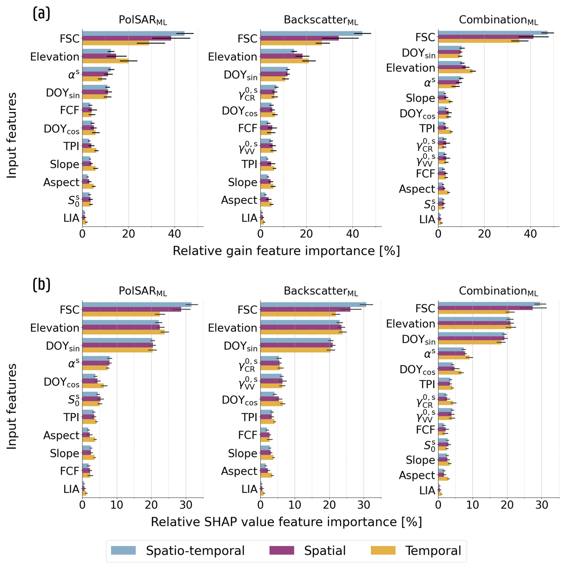
Figure 4 Feature importance for the PolSAR_ML, Backscatter_ML and Combination_ML configurations, indicating the strong influence of FSC, elevation and DOY on the model outcome (a, b), the elevated usage of α^s and ${\mathit{\gamma }}_{\text{VV}}^{\text{0,s}}$ during SD prediction (b), and the preference of the Combination_ML configuration for α^s over ${\mathit{\gamma }}_{\text{CR}}^{\text{0,s}}$ (a, b). Upper row (a): Relative gain-based FI. Bars represent the mean FI across the XGBoost models trained during inner resampling, with colors indicating the type of nested CV framework. Lower row (b): Similar to (a), but here FI is quantified as the mean absolute SHAP value per feature (relative values), computed separately for each test fold during outer resampling. The black lines in the bars denote the 95 % confidence interval.

When used in the separate configurations, the S1 PolSAR and backscatter intensity features are similarly used during model training (Fig. 4a). However, the gain FI indicates a stronger importance of α^s within the PolSAR_ML configuration over ${\mathit{\gamma }}_{\text{CR}}^{\text{0,s}}$ in the Backscatter_ML one. This observation is further confirmed in Fig. 4b across all nested CV frameworks, indicating that XGBoost seems to effectively extract more information from α^s during model training and SD prediction. Consistent with this finding, the Combination_ML configuration also exhibits a clear preference of α^s over ${\mathit{\gamma }}_{\text{CR}}^{\text{0,s}}$. In addition, both the gain-based and SHAP value FI analyses reveal a less distinct separation between the S1 input features in the Backscatter_ML configuration, with the SHAP values even suggesting that ${\mathit{\gamma }}_{\text{VV}}^{\text{0,s}}$ contributes as much as, or slightly more than, ${\mathit{\gamma }}_{\text{CR}}^{\text{0,s}}$ during SD prediction at unseen locations and/or time periods.

SHAP value analysis during snowpack presence

The SHAP value FI of the S1 variables (Fig. 4b) were further evaluated during snow-covered periods – encompassing both wet and dry snow periods – within the spatial nested CV framework, as this framework matches best with the objective of the study: SD prediction across the Alps using the available S1 archive. Figure 5a presents the FI for both the full set of predictions (fully colored bars), and the subset remaining after excluding the non-valid areas masked within the wet snow product (dark gray lines). Excluding the non-valid areas increases the overall and dry-period FI for both α^s and ${\mathit{\gamma }}_{\text{CR}}^{\text{0,s}}$ within the PolSAR_ML and Backscatter_ML configuration, respectively. As these non-valid areas include low-elevation areas (i.e., valleys) and densely-forested regions, locations where typically low SD values are observed, these results suggests that XGBoost places relatively more importance on these S1 variables at bare, higher-elevation locations that are often characterized by deeper snowpacks. Conversely, the decrease in SHAP value FI when including these non-valid areas indicates the limited added value of the S1 variables to predict SD at low-elevation and/or densely-forested sites. Although no valid wet-snow classification is available for such areas (e.g., Fig. 5d where only low FCF values appear for the wet-snow subplot) and more advanced classification approaches incorporating meteorological data could enable a more accurate separation of dry and wet snow periods, we argue that the current analysis is sufficient given the limited contribution of S1 variables in these environments. This marginal contribution was also reported by Dunmire et al. (2024) and is further evident in Fig. C1d. As this limitation arises from the raw S1 observations rather than the type of processed S1 observations (i.e., PolSAR vs. backscatter intensities), this limitation should be addressed by incorporating additional input features (e.g., Fig. C2).

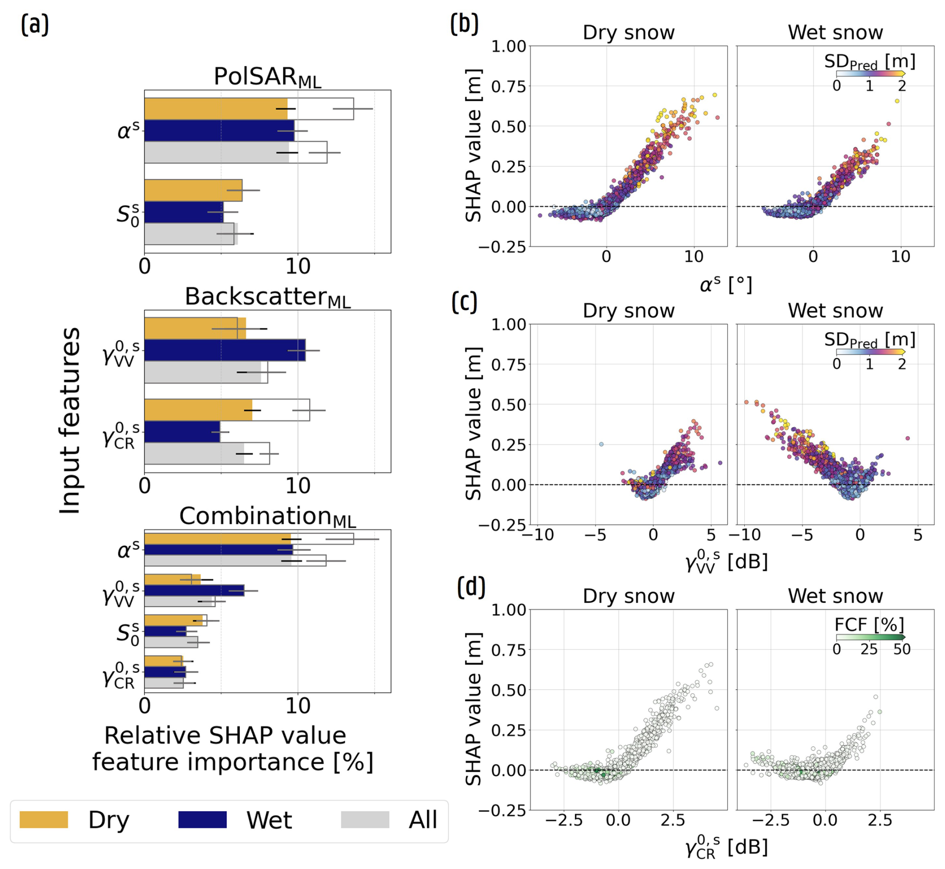
Figure 5 SHAP value analysis for the spatial nested CV framework during snow presence, indicating XGBoost's stronger reliance of, and preference for, α^s compared to ${\mathit{\gamma }}_{\text{CR}}^{\text{0,s}}$, and the notable use of ${\mathit{\gamma }}_{\text{VV}}^{\text{0,s}}$ during wet snow periods. (a) Relative SHAP value FI of the satellite input features for the PolSAR_ML, Backscatter_ML and Combination_ML configurations. The dark gray lines represent the FI after masking out non-valid dry snow classifications. (b) Scatter plot of mean α^s values and corresponding SHAP values for the PolSAR_ML configuration, taken as the mean per site and snow season during dry and wet snow conditions (only valid classifications). The dots are colored according to the mean predicted SD (SD_pred). (c) Same as (b), but for ${\mathit{\gamma }}_{\text{VV}}^{\text{0,s}}$ within the Backscatter_ML configuration. (d) Same as (c) for ${\mathit{\gamma }}_{\text{CR}}^{\text{0,s}}$, but colorized to the site FCF, indicating that the classification primarily targets higher-elevation non-forested areas.

Figure 5a also explains the more pronounced difference in SHAP value FI between the PolSAR variables, as XGBoost relies more heavily on α^s than on $S_{\mathrm{0}}^{\mathrm{s}}$ across all snow conditions. In contrast, the Backscatter_ML configuration places greater emphasis on ${\mathit{\gamma }}_{\text{VV}}^{\text{0,s}}$ than on ${\mathit{\gamma }}_{\text{CR}}^{\text{0,s}}$ during wet snow conditions, which accounts for their nearly equivalent overall SHAP value FI (Fig. 4). In addition, the FI patterns observed in the Combination_ML configuration closely resemble those of the PolSAR_ML and Backscatter_ML configurations, with the notable exception of ${\mathit{\gamma }}_{\text{CR}}^{\text{0,s}}$. Here, XGBoost seems to rely more heavily on α^s at the expense of ${\mathit{\gamma }}_{\text{CR}}^{\text{0,s}}$, which was also evident from Fig. 4, and is also observed at a measurement site located near Prato, Switzerland (46.47° N, 8.72° E; Fig. C1c). Similar observations were made by Jans et al. (2025), who reported stronger correlations between α and modeled SD during the accumulation (dry snow) period at most locations in their study area than between modeled SD and ${\mathit{\gamma }}_{\text{CR}}^{\mathrm{0}}$. In addition, S₀ shows a similar SHAP value FI importance as γ_VV during dry snow conditions (Fig. 5a, Combination_ML configuration), and is even more important at bare high-elevation sites (dark gray lines), further confirming the findings of Jans et al. (2025). In contrast, γ_VV is more extensively used during wet snow conditions, resulting in the slightly higher observed overall FI for this S1 variable.

Within the PolSAR_ML configuration (Fig. 5b), XGBoost has learned a positive relationship between α^s and its contribution to the SD estimates, consistent with the findings of Jans et al. (2025), who reported increasing α-values with dry snowpack accumulation at sites where the S1 signal penetrates the snowpack at oblique incidence angles (medium to high LIA). However, at certain medium–high elevation sites (1500–2500 m; e.g., Fig. C1b), both α^s and its SHAP value contributions remain low or even negative (Fig. C1b) despite relatively high predicted and observed SD. Instead, increases in ${\mathit{\gamma }}_{\text{VV}}^{\text{0,s}}$ or $S_{\mathrm{0}}^{\mathrm{s}}$ are observed, a pattern shown to be more prevalent at sites with low-LIA satellite overpasses (Jans et al., 2025) where the S1 signal penetrates the snowpack more vertically and decreasing α-values are observed. Nevertheless, these patterns may also occur at locations with medium-LIA S1 observations (e.g., the site in Fig. C1b that shows increasing ${\mathit{\gamma }}_{\text{VV}}^{\text{0,s}}$-values) and further research is required to understand their origin. In addition, these patterns help explain the dual relationship observed for ${\mathit{\gamma }}_{\text{VV}}^{\text{0,s}}$ in Fig. 5c: at certain locations, a limited positive contribution is found, whereas at the majority of sites, a strong inverse relationship emerges during wet snow conditions, when a decrease in this S1 variable is typically observed (e.g., Fig. C1a). Finally, Fig. 5b and d illustrate that under wet snow conditions, α^s remains more elevated compared to ${\mathit{\gamma }}_{\text{CR}}^{\text{0,s}}$, leading to higher associated α^s SHAP values in the PolSAR_ML configuration than the corresponding ${\mathit{\gamma }}_{\text{CR}}^{\text{0,s}}$ SHAP values in the Backscatter_ML configuration. This suggests that SD estimation based on α^s might be less sensitive to the presence of liquid water than SD estimation based on ${\mathit{\gamma }}_{\text{CR}}^{\text{0,s}}$.

4.3 Added value of meteorological forcings and Snowclim SD estimates

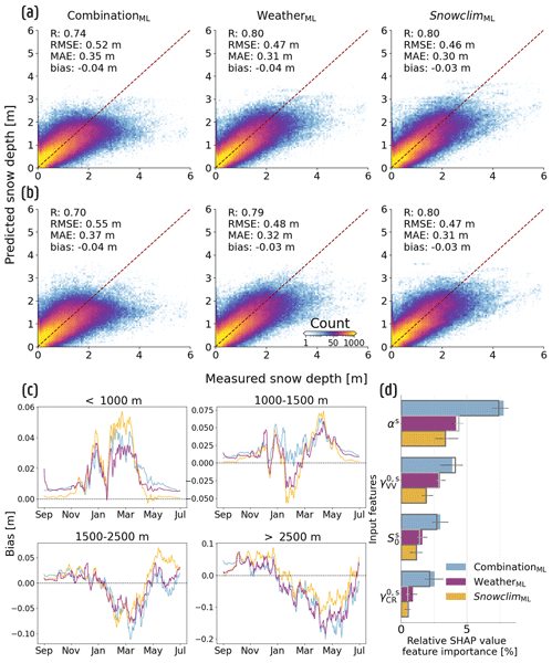
Figure 6 illustrates the improvements when incorporating either regionally downscaled meteorological forcing data or Snowclim SD estimates (Table 2; Weather_ML and Snowclim_ML configurations) when predicting at unseen locations (and time periods; Fig. 6a and b), with the most important improvements for high SD observations (≥2.5 m). The bias for observations ≥2.5 m improves by 28 cm when comparing the Weather_ML to the Combination_ML configuration within the spatial nested CV framework (Fig. 6a), decreasing from −1.48 to −1.20 m. Incorporating Snowclim SD estimates further reduces this bias to −1.12 m, likely reflecting a stronger correspondence between the Snowclim estimates and high SD observations than what is captured through derived meteorological variables. Despite these gains, the number of sites with a mean bias $\le -\mathrm{0.5}$ m remains similar in both the Weather_ML and Snowclim_ML configurations – with most of these sites again located in Switzerland (Fig. E2) – reflecting the need for expanded high SD data collection. Furthermore, while the inclusion of meteorological forcing data or modeled SD estimates reduces the relative SHAP value FI of the S1 input features, these features continue to influence SD predictions (Fig. 6d), accounting in total for approximately 9 % and 7 % of the SHAP value FI in the Weather_ML and Snowclim_ML configurations, respectively, when predicting at unseen locations.

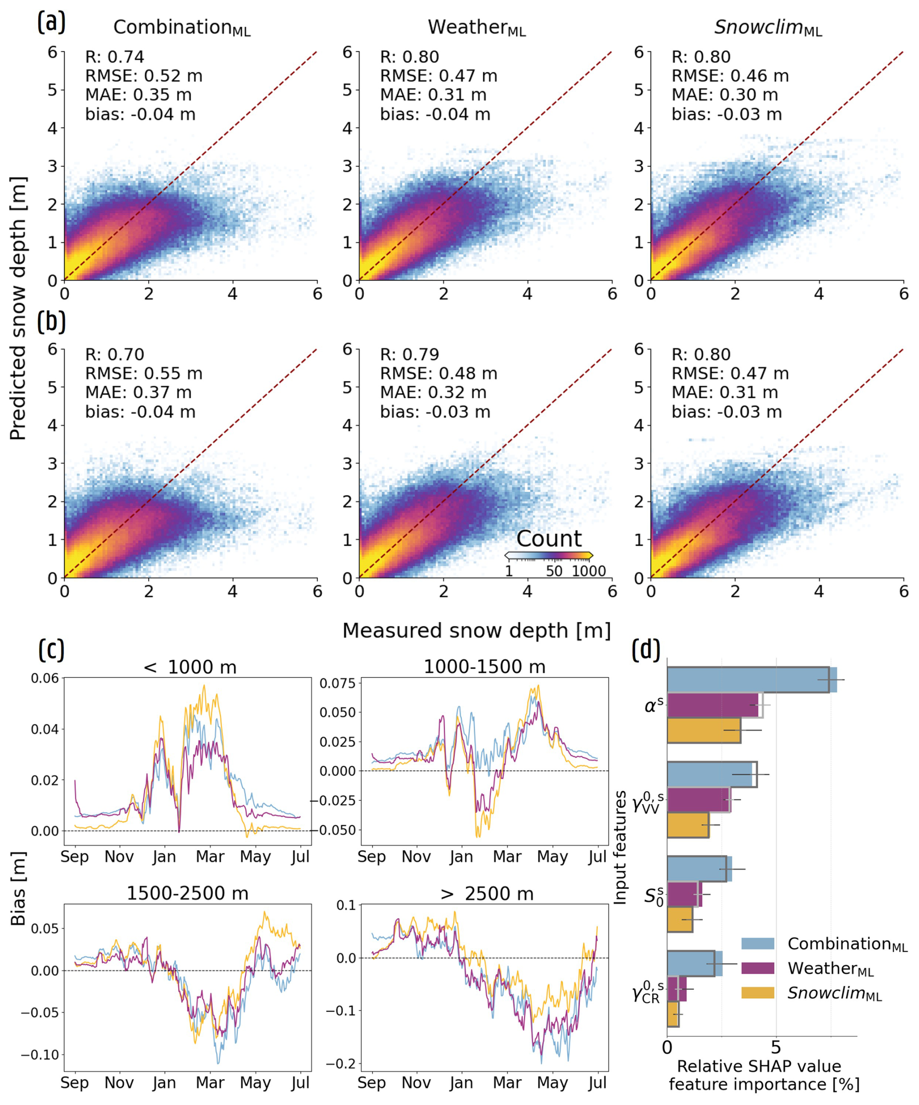
Figure 6 Improvements brought by additional input of meteorological forcing data or Snowclim SD estimates when predicting at unseen locations and time periods. (a) 2D histograms of measured vs. predicted SD for the Combination_ML, Weather_ML, and Snowclim_ML configurations for the spatial nested CV framework. Performance metrics are computed with exclusion of zero-measured SD. (b) Same as (a), but for the spatio-temporal framework. (c) 7 d mean bias (including zero-measured SD) over the course of a general snow season, for different elevation classes. (d) Relative SHAP value FI for the different configurations for the spatial (full colored bars) and the spatio-temporal nested CV framework (gray line).

Overall, the Snowclim_ML configuration yields the best performance (Fig. 6a and b). Under the spatio-temporal nested CV framework, site-MAE during snow-covered periods decreases by at least 2.5 cm at 55 % of sites, while only 16 % exhibit an increase of 2.5 cm or more, relative to the Combination_ML configuration. Compared to the Weather_ML configuration, the difference in site-MAE is minimal, and only significant for the spatio-temporal framework. However, the Snowclim SD estimates appear to more accurately represent conditions at low-elevation sites (<1000 m) during the early snow season (Fig. 6c), highlighting the importance of reliable FSC information to correctly indicate snow-free conditions when relying solely on meteorological forcing data. In addition, while the Weather_ML configuration displays the lowest bias of the three configurations at medium-elevation (1000–2500 m) sites (Fig. 6c), the Snowclim_ML configuration still performs best at high-elevation sites (>2500 m) during peak SD and the ablation period. Nonetheless, both the Weather_ML and Snowclim_ML configurations seem to underestimate SD near March–May, with the differences being less pronounced for the 1500–2500 m elevation class. As such, the results indicate that directly using meteorological forcings can achieve comparable predictive performance within the applied XGBoost setup. This would eliminate the need to run a snow model, which reduces both computational cost and model complexity.

4.4 Spatial SD prediction

To address the findings of López-Moreno et al. (2015) and Miller et al. (2022), who emphasized that stationary and point-based SD measurements inadequately capture spatial snowpack variability, we trained the Combination_ML, Weather_ML and Snowclim_ML configurations with additional spatially distributed SD training (survey) data, and compared its impact over the Dischma valley. Figure 7a–c display the results of the 16 March 2017 snow survey (Fig. 7d), in which mountain ridges appear more distinctly in the predictions, and high SD estimates at steep locations and near ridges are more accurately corrected compared to Fig. E3a–e, which depict results obtained without spatial training data. Negative adjustments can be observed at high-elevation areas with (relatively) steep slopes for all configurations, but is most pronounced for the Combination_ML configuration (Appendix D). For the latter, the negative corrections are reflected in a reduced SHAP value FI of the topographic inputs (Fig. 7h, survey data; Appendix D). In contrast, the SHAP value FI of the topographic inputs increases in the Weather_ML and Snowclim_ML configurations (Fig. 7i and j). Here, the topographic features contributed less when the models were trained solely on point-based measurements but become increasingly influential once spatial training data are included, enabling improved representation of topographic controls on the SD estimates. Notably, α^s remains among the more influential features for these configurations, indicating that despite its reduced relative importance, the inclusion of this S1 variable (and potentially other S1 variables) continues to affect the final SD predictions.

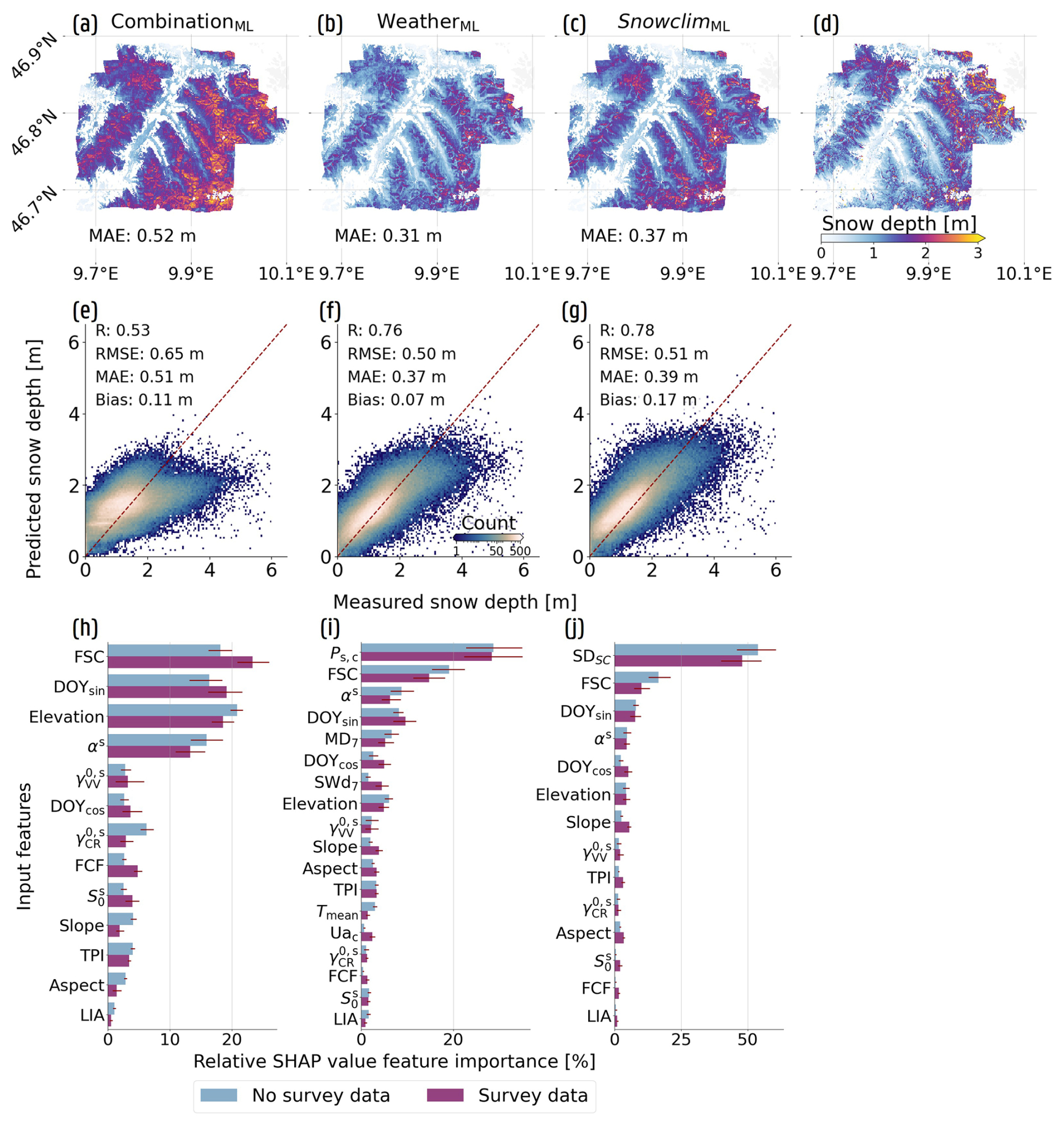
Figure 7 Improvements obtained by incorporating spatially distributed SD training data when predicting across the Dischma Valley (Switzerland), including their impact on SHAP-based FI. The first column (a, e, h) represents the results for the Combination_ML configuration, while the second (b, f, i) and third column (c, g, j) show the results for the Weather_ML and Snowclim_ML configurations, respectively. (a), (b) and (c) display the spatial predictions for the 16 March 2017 snow survey, with (d) representing the measured SD. (e), (f) and (g) show 2D histograms and performance metrics across all nine conducted snow surveys. Finally, (h), (i) and (j) display relative SHAP value FI, both when trained with or without spatial SD (survey) data. The 95 % confidence interval is indicated with a red bar.

Despite the improvements, SD remains overestimated for the 16 March 2017 snow survey across all configurations. This overestimation is most pronounced for the Combination_ML configuration and exceeds the bias reported by Dunmire et al. (2024). Although it is not the objective of this study to perform a direct comparison, the persistence of the Combination_ML bias indicates potential limitations in the current feature selection or training dataset. Nonetheless, both the Weather_ML and Snowclim_ML configurations outperform the results reported by Dunmire et al. (2024). For the 9 March 2016 and 16 March 2017 snow surveys used by Dunmire et al. (2024) for model validation, the Weather_ML and Snowclim_ML configurations achieve higher correlation coefficients (0.68 and 0.64) and lower mean absolute errors (31 and 36 cm, respectively) than those reported by Dunmire et al. (2024) (0.56 and 41 cm). For the 16 March 2017 survey specifically, Dunmire et al. (2024) reported a mean SD difference (predicted minus observed) of 16 cm, whereas the Weather_ML and Snowclim_ML configurations exhibit differences of −5 and 15 cm, respectively. Thereby, the more pronounced overestimation of the Snowclim_ML configuration likely results from the systematic overestimation in the Snowclim SD estimates for this survey (Fig. D2d), which may also explain the 6 cm higher MAE compared to the Weather_ML configuration (Fig. 7b and c).

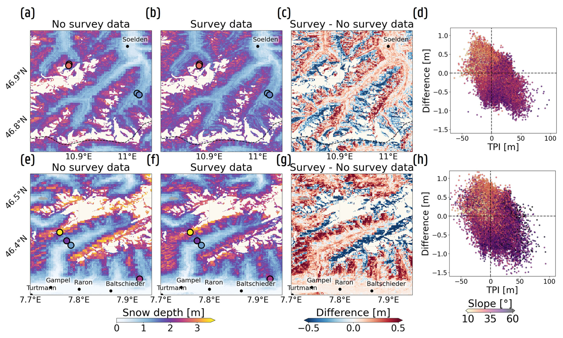
Figure 8 Improved representation of topographical controls on SD estimates for the Weather_ML configuration on 29 January 2018 over the Ötztal, Austria (top row) and the Lötschental, Switzerland (bottom row). (a, e) Mean SD estimates predicted with the nine separately trained XGBoost models utilizing no spatial (No survey) training data. (b, f) Same as (a, e), but with inclusion of spatial SD training data (Survey). (c, g) Difference maps between the mean SD predictions, trained with and without spatial SD training data. (d, h) Scatter plots of TPI and SD differences, colored according to slope. Observed SD at the stationary sites are displayed in (a), (b), (e) and (f) as dots. Glaciers and lakes located within the valleys are colored in white and dark gray, respectively, and are excluded from the analyses.

Across the nine snow surveys, the inclusion of spatially distributed SD training data primarily improves predictions for lower observed SD values (Fig. 7 and E3e–g), whereas differences for higher SD observations (≥2.5 m) remain less pronounced, albeit best captured by the Snowclim_ML configuration. Despite a persistent positive bias across all configurations, the Weather_ML configuration exhibits a bias reduction of approximately 10 cm relative to the Snowclim_ML configuration, suggesting that explicitly running Snowclim may not be required when the primary objective is to obtain accurate SD estimates across the European Alps. Indeed, XGBoost effectively learns the relationship between the meteorological forcing data and observed SD, without explicitly representing the physical processes governing snowpack evolution. For the Snowclim_ML configuration, the remaining overestimation largely originates from biases in the Snowclim SD estimates themselves (Figs. B1b and D2d). In contrast, the origin of the positive bias in the Weather_ML configuration is less straightforward and may reflect either an overestimation of cumulative snowfall (P_s,c) or limitations in XGBoost’s ability to implicitly represent variations in snow bulk density. In the latter case, even accurate snowfall forcing may still result in SD overestimation due to an implicit underrepresentation of snow densification processes. Further research should attempt to include factors or use ML models that govern variations in snow density, especially to enhance the potential of predicting short-term variations in SD. Finally, elevation mismatches within the relatively coarse 500 m meteorological forcing data may introduce temperature biases, thereby affecting snowfall estimates and the inferred number of melt days.

Figure 8 further illustrates the impact of the spatial training data outside the Dischma valley. The top row displays the SD estimates across the Ötztal region (Austria) on 29 January 2018, while the bottom row showcases the results for the Lötschental region (Switzerland), on the same date. For both valleys, the inclusion of spatial training data improved the spatial patterns, manifested by the appearance of mountain ridges and local depressions (Fig. 8b and f). These patterns also appear in the difference maps (Fig. 8c and g), and seem to be related to the TPI (Fig. 8d and h). Specifically, Fig. 8d and h indicate that SD estimates at areas situated below their surroundings (negative TPI) are positively corrected, whereas the opposite is true near mountain ridges. Figure 8d and h moreover indicate a dependency with the slope of the area, with steeper areas exhibiting more pronounced negative corrections, while flatter regions show the opposite tendency. The relationship with the other topographic features (e.g., aspect), however, is less clear.

5 Conclusions

An extreme gradient boosting model (XGBoost) was applied to assess whether the integration of Sentinel-1 (S1) C-band synthetic aperture radar (SAR) dual-polarized polarimetric (PolSAR) observations – either as a replacement for, or in combination with S1 backscatter intensity observations – improves SD predictions across the European Alps relative to a backscatter-intensity-based configuration. In addition, two extended configurations were evaluated in which the S1 observations were supplemented with either meteorological forcing data or SD estimates from the process-based Snowclim model, to assess both the associated performance gains and the continued contribution of S1 observations to SD prediction. Results were evaluated at locations and/or during time periods not covered by the training data using a threefold nested cross-validation (nested CV) scheme, while feature importance analysis was employed to assess the contribution of the different input variables during both dry and wet snow periods. In addition, nine photogrammetry snow surveys were used to validate the spatial prediction capacity of the configurations.

Our results show modest improvements in estimated SD with the inclusion of S1 C-band PolSAR observations, with gains primarily observed in site-level performance under spatio-temporal generalization, whereas no significant improvements are found in these metrics under spatial generalization alone. However, feature importance analysis indicates a stronger reliance on the polarimetric scattering angle (α) than the cross-polarization ratio (${\mathit{\gamma }}_{\text{CR}}^{\mathrm{0}}$), during both dry and wet snow periods, while the drop in co-polarized (VV) backscatter intensity (${\mathit{\gamma }}_{\text{vv}}^{\mathrm{0}}$) seems to be actively used during the ablation period. Incorporating meteorological forcing data or Snowclim SD estimates further improved XGBoost's performance substantially, while the model continued to make use of information from the S1 observations, particularly α. Nonetheless, high SD observations remain systematically underestimated, primarily due to their limited representation in the training dataset. Finally, our results depict the importance of spatially distributed SD training data to capture topographic variability, reflected through a negative relationship between topographic position index (TPI) and adjustments in SD estimates relative to predictions from XGBoost trained without spatial training data.

Despite these advances, SD values above approximately 2.5 m remain underestimated, emphasizing the need for more extensive snow monitoring and additional spatial snow surveys within the European Alps. Furthermore, XGBoost operates at the pixel level and cannot inherently capture dependencies between adjacent pixels; instead, spatial context must be explicitly incorporated through engineered features. Finally, while improving SD estimates is a step toward addressing snow mass knowledge gaps, future research should focus on direct snow mass estimation and integrating spatial dependencies through methods that incorporate information from adjacent pixels.

Appendix A: Combining Terra and Aqua fractional snow cover data

To generate a combined daily fractional snow cover (FSC) product from the MODIS Terra and Aqua satellites, we applied a weighted averaging approach to merge the individual satellite observations. As such, we calculated for each location i and day t the weights of the individual FSC data ($W_{{\text{sat}}_{i,t}}$) using the following formula:

$$\begin{array}{}\text{(A1)}& {\displaystyle }{W}_{{\text{sat}}_{i,t}}{\displaystyle }={\displaystyle \frac{\mathrm{1}}{W_{\text{QA}}\cdot W_{\text{CP}}\cdot W_{\text{DD}}}}\end{array}$$

in which W_QA is the weight associated with the quality flag (QA, that ranges between 0 and 2 with 0 indicating the highest quality) of the satellite data; W_CP is the weight based on the number of days since the last cloud-free observation (CP; values between 0 and ∞); and W_DD is the weight accounting for the difference in days between the most recent cloud-free Terra and Aqua observations (DD; values between 0 and ∞, where 0 corresponds to the satellite with the most recent cloud-free data). The individual weights were computed using the following formulations, which were designed to ensure that none of the weights attain zero:

$$\begin{array}{}\text{(A2)}& {\displaystyle }{W}_{\text{QA}}& {\displaystyle }={\displaystyle \frac{\mathrm{1}}{\text{QA}+\frac{(\mathrm{2}-\text{QA})}{\mathrm{2}}}}\text{(A3)}& {\displaystyle }{W}_{\text{CP}}& {\displaystyle }={\displaystyle \frac{\mathrm{1}}{(\text{CP}+\mathrm{1}{)}^{\mathrm{2}}}}\text{(A4)}& {\displaystyle }{W}_{\text{DD}}& {\displaystyle }={\displaystyle \frac{\mathrm{1}}{(\text{DD}+\mathrm{1})}}\end{array}$$

Appendix B: Snowclim parameter settings and performance

Snowclim model parameters were calibrated with a two-step approach, involving a subset of the snow dataset. First, we identified the best working downscaling techniques – multiple options were assessed to downscale temperature, precipitation, relative humidity, and downward shortwave radiation – by comparing model performance with measured SD using the standard parameter set used by Lute et al. (2022) (Table 2, superscript ^c) in their full model run. Next, we used the downscaled forcing data to select the optimal parameters out of 1276 tested combinations, by applying a similar approach as described in Lute et al. (2022). A list of the final calibrated parameters is provided in Table B1.

Table B1 Parameter settings used to generate SD estimates across the European Alps. For the detailed description of the separate parameters, we refer to Lute et al. (2022).

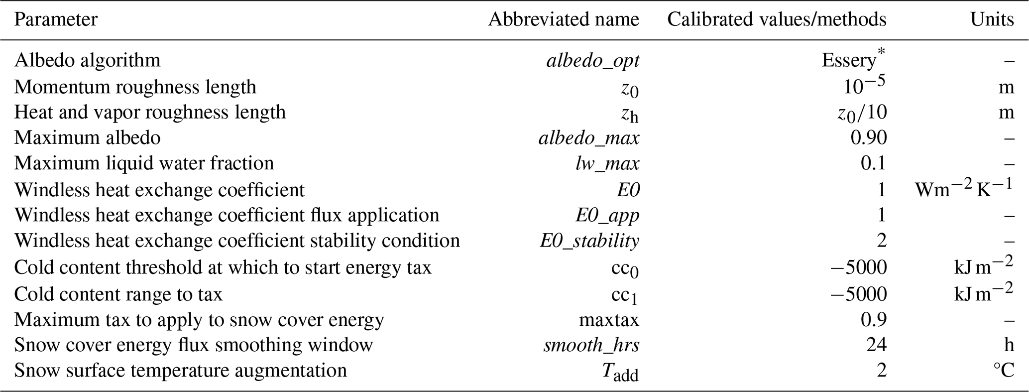
^* Essery et al. (2013).

Figure B1 shows the performance across the SD dataset, for (a) data from the stationary and point-based measurements, and (b) the Dischma valley photogrammetry snow surveys. Performance metrics are computed excluding zero-measured SD. When zero values and both stationary site and survey data are included, the Pearson correlation coefficient is 0.84, while the RMSE and MAE display values of 0.64 and 0.40 m, respectively. Compared to the stationary sites alone, the Snowclim SD estimates show higher accuracy, with an MAE of 0.40 m (excluding zero-measured SD). In contrast, when only the nine photogrammetry snow surveys are compared with the corresponding Snowclim estimates, the MAE deteriorates to 0.80 m.

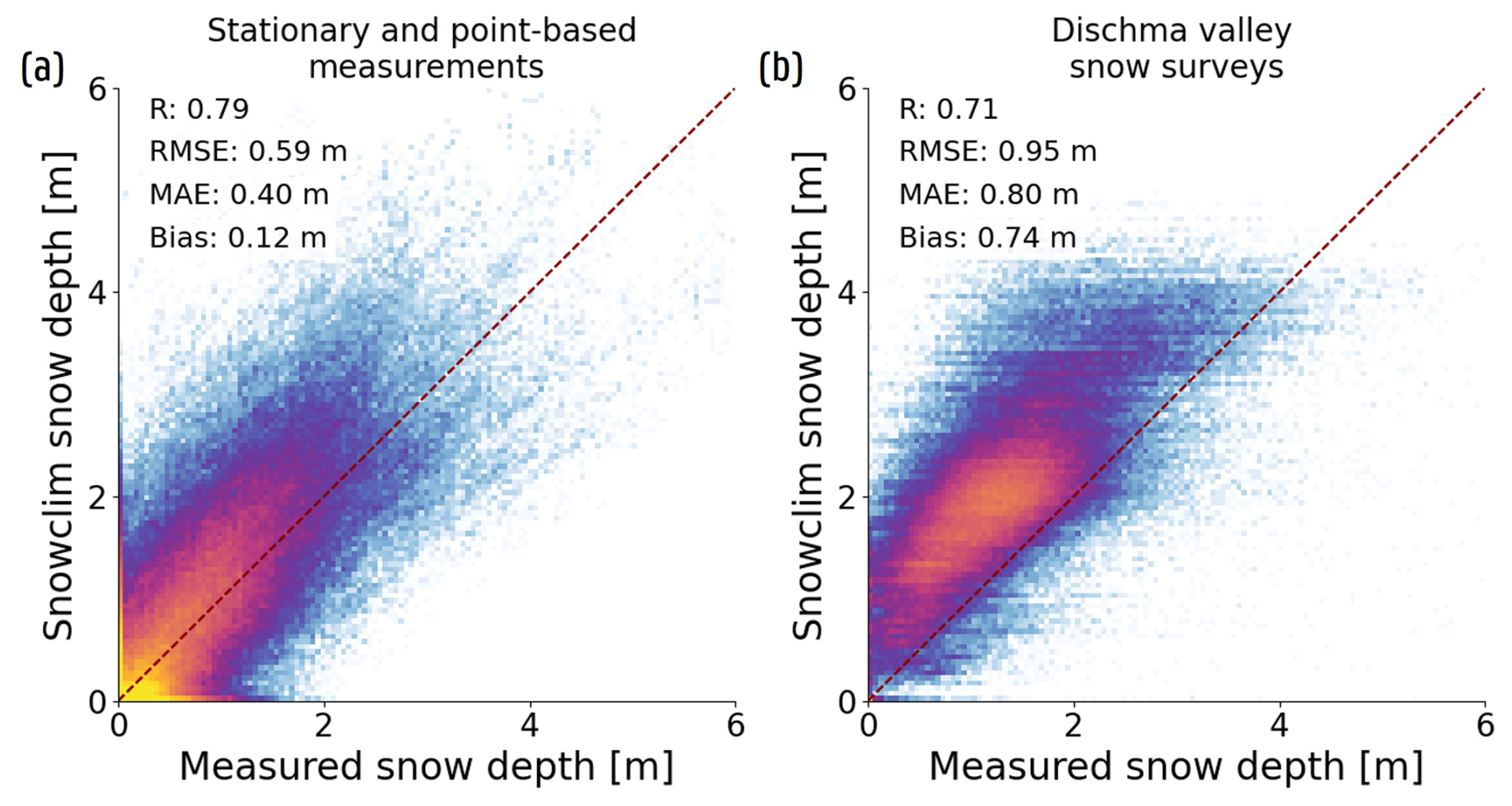
Figure B1 Performance of the process-based model Snowclim for the snow measurements dataset, indicating a general overestimation, particularly for the Dischma valley snow surveys. (a) 2D histogram comparing measured SD at the stationary sites with the Snowclim SD estimates. (b) Same as (a), but for the nine Dischma valley snow surveys. Displayed performance metrics do not incorporate zero-measured SD.

Appendix C: Time series of SD and SHAP values

The SHAP value contributions of the S1 variables within the Combination_ML configuration were assessed during the 2017–2018 and 2018–2019 snow seasons at four distinct sites in Switzerland (Fig. C1). All sites are operated by the Swiss Institute for Snow and Avalanche Research (SLF; Sect. 2.1), and the results shown correspond to the spatial nested CV framework. Figure C1a shows the time series for a measurement site near Arolla, Valais (46.41° N, 8.92° E), located in a bare rock area with a 0 % FCF and surrounded by mountains to the east, north, and west. At this high-elevation and bare site, the added value of α^s under dry snow conditions and ${\mathit{\gamma }}_{\text{VV}}^{\text{0,s}}$ under wet snow conditions becomes clear. During the 2017–2018 snow season, namely, a clear increase in α^s is observed during the accumulation phase. After reaching peak values around late January, associated with a large snowfall event, α^s and its associated SHAP values remain elevated until the snowpack starts to wet near the end of March. However, the peak occurs before the maximum measured SD in early April, a phenomenon not unique to this site and also reported by Jans et al. (2025), who found an average lag of around 60 d between peak α and peak SD in their study area. In contrast, the observed ${\mathit{\gamma }}_{\text{VV}}^{\text{0,s}}$ values do not increase during the accumulation phase, consistent with the findings of Lievens et al. (2019), and contribute minimally to the SD predictions. At certain sites – usually with low-LIA satellite overpasses – however, ${\mathit{\gamma }}_{\text{VV}}^{\text{0,s}}$ and it's SHAP values do increase during the accumulation period (e.g., a site near Grindelwand shown in Fig. C1b). As such, depending on the LIA, α^s and ${\mathit{\gamma }}_{\text{VV}}^{\text{0,s}}$ might contribute more or less to the predictions during dry snow conditions.

During the ablation phase, marked by a decline in ${\mathit{\gamma }}_{\text{VV}}^{\text{0,s}}$ in early April, the contribution of α^s drops sharply, in line with decreasing observed values. In contrast, ${\mathit{\gamma }}_{\text{VV}}^{\text{0,s}}$ emerges as the most informative S1 feature under these wet snow conditions, with positive SHAP values peaking near its lowest observed backscatter intensities. Beyond this point, as ${\mathit{\gamma }}_{\text{VV}}^{\text{0,s}}$ increases due to the growing influence of superficial scattering processes (Marin et al., 2020), the contribution gradually declines. Similar patterns have been observed at other sites (e.g., 46.42° N, 8.23° E and 46.39° N, 7.97° E) and is also evident from Fig. 5c. In contrast, the behavior of α^s and its contribution to the SD estimates during the ablation period is less consistent. At some sites (e.g., 46.08° N, 7.92° E), the drop in ${\mathit{\gamma }}_{\text{VV}}^{\text{0,s}}$ coincides with a sudden increase in α^s, whereas at other sites, no such increase is observed or an increase is linked to late-season snowfall events. Further research is required to better understand the interaction between wet snow and α, though this is beyond the scope of this study.

The Arolla site (Fig. C1a) shows a similar seasonal evolution of ${\mathit{\gamma }}_{\text{VV}}^{\text{0,s}}$ in 2018–2019 as in 2017–2018, further supporting the findings of Fig. 5 on the role of this S1 feature under different snow conditions. In contrast, although α^s increases slightly in mid-March, it begins to decline as early as late February, whereas no corresponding sharp decrease is observed in ${\mathit{\gamma }}_{\text{VV}}^{\text{0,s}}$. While difficult to confirm, this may be related to melt-freeze events and/or metamorphism processes happening in the snowpack starting in early March. Nevertheless, α^s also here strongly contributes during snow accumulation, when it is most informative.

The potentially added value of α^s to the SD predictions at higher-elevated, bare locations is further supported by Fig. C1c, that displays the time series at a measurement site located near Prato, Ticino (46.47° N, 8.72° E), with a similar 0 % FCF but lower elevation (2222 m above sea level (m a.s.l.)). Unlike the Arolla site, however, α^s is not only mainly informative during snow accumulation, but remains relatively elevated throughout February and March for both snow seasons, when the snowpack exceeds 2 m of snow. Nonetheless, the SD predictions appear to level off with only a limited response to new snowfall events, which is observed at the Arolla site during the 2017–2018 snow season as well. One explanation lies in the limited number of high SD observations used to train XGBoost (Fig. E1a), which constrains the model’s ability to represent higher SD values and results in a flattening of the predicted SD range (Fig. 6a). Differently, there might be a saturation, or even already a decrease, in the S1 variables that respond to increasing SD at the beginning of the snow season, so that XGBoost cannot rely on these features to account for new snow events. This leveling-off should be taken into account when deploying XGBoost to predict SD across the Alps, especially when relying solely on S1 variables and FSC to explain interannual variability. Additionally, Fig. C1c helps to explain the relative SHAP value FI of ${\mathit{\gamma }}_{\text{CR}}^{\text{0,s}}$ in the bottom panel of Fig. 5a. Although XGBoost captures the increase in ${\mathit{\gamma }}_{\text{CR}}^{\text{0,s}}$ during the accumulation period to contribute positively to the predicted SD, the SHAP value contribution is way smaller compared to α^s, indicating a preference for α^s over ${\mathit{\gamma }}_{\text{CR}}^{\text{0,s}}$ by XGBoost.

Finally, the bottom time series (Fig. C1d) corresponds to a forested (63 % FCF, 1868 m a.s.l.) site in Sobrio, Ticino (46.41° N, 8.92° E). Despite being consistently classified as dry snow in the time series, this area is actually masked as forest in the CLMS SWS wet snow product. This site was also analyzed by Dunmire et al. (2024), who concluded that, given the low FI of ${\mathit{\gamma }}_{\text{VV}}^{\text{0,s}}$ and ${\mathit{\gamma }}_{\text{CR}}^{\text{0,s}}$ in their study, S1 satellite observations should not be used for this location. Our findings support the limited contribution of the S1 features at similar lower and/or forested areas, as we observe minimal added value from both α^s and ${\mathit{\gamma }}_{\text{VV}}^{\text{0,s}}$ at this site. Within such sites, the predictions from XGBoost trained without satellite observations (No S1) are similar to, or even outperform, those based on satellite inputs (Fig. C2). Differently, additional inputs such as meteorological forcings can also improve the results (Fig. C2).

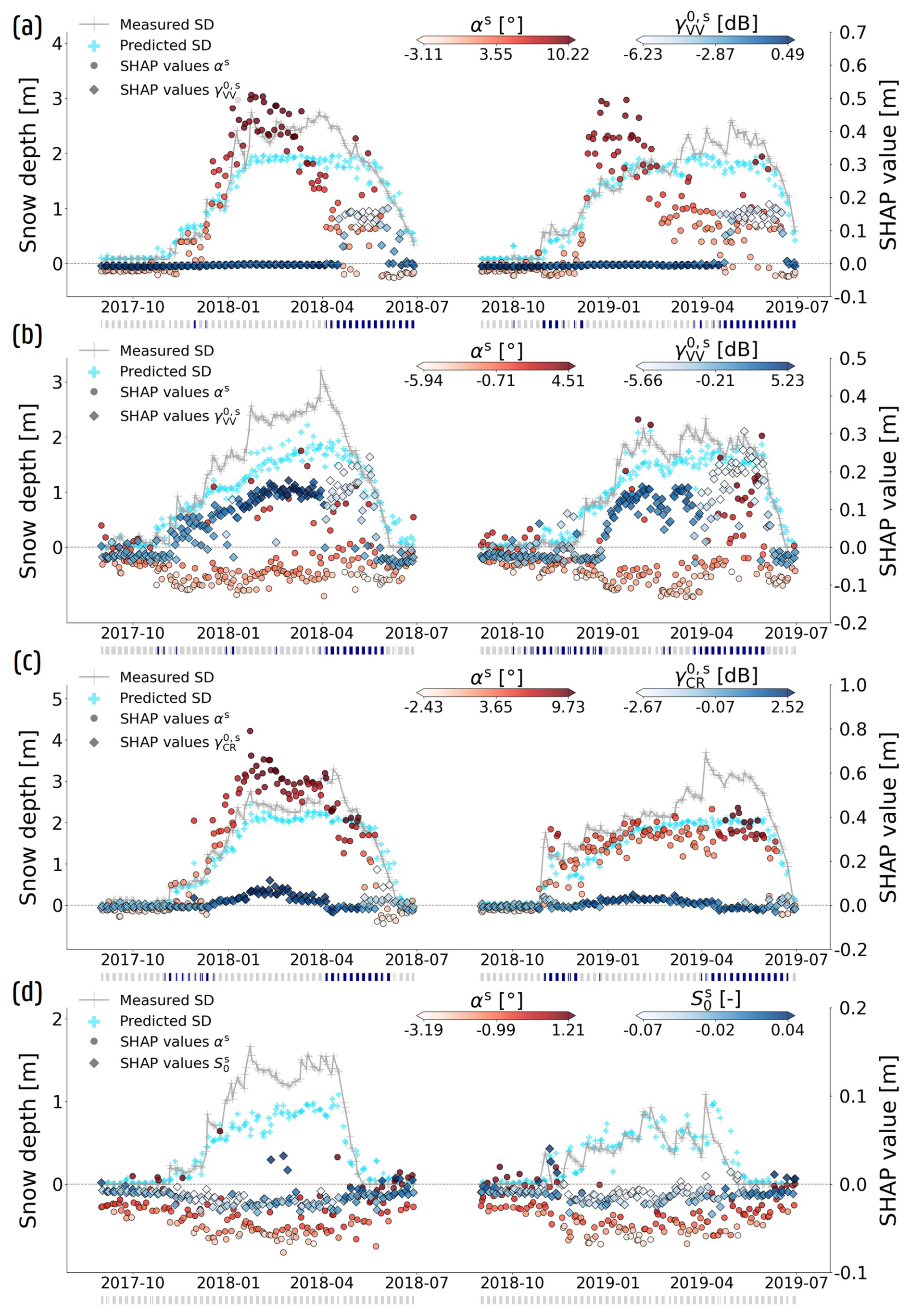
Figure C1 SD predictions (spatial nested CV framework) and associated contribution of various S1 input features for the 2017–2018 and 2018–2019 snow seasons, at four SLF sites within Switzerland: (a) Arolla: 46.41° N, 8.92° E, (b) Grindelwand: 46.67° N, 8.06° E, (c) Prato: 46.47° N, 8.72° E, and (d) Sobrio: 46.41° N, 8.92° E. Measured SD is shown in gray, while predictions are denoted by light blue crosses. SHAP values for two S1 variables, representing their contribution in time, are plotted as well, and colored according to their input value in XGBoost. The stripes below the time series indicate dry (light gray) or wet (dark blue) snow conditions according to CLMS SWS wet snow product.

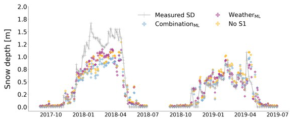
Figure C2 Time series for the spatial nested CV framework at an SLF site near Prato, Ticino in Switzerland (46.41° N, 8.92 E), displaying the added value of meteorological forcings, and the performance without inclusion of S1 variables. The time series display measured (gray) and predicted (crosses) SD for the 2017–2018 and 2018–2019 snow seasons. The colors indicate the configuration used: Combination_ML (blue), Weather_ML (purple) and a configuration using no S1 variables, nor meteorological forcings or Snowclim SD estimates (No S1; yellow).

Appendix D: 16 March 2017 Dischma valley snow survey SD estimates

Figure D1 illustrates differences in predicted SD values for the Combination_ML configuration trained without (No survey; b) and with (Survey; c) spatially distributed SD training data. Although substantial overestimation persists after incorporating spatial SD training data, excessively high SD predictions at steep slopes and near mountain ridges are more effectively corrected. Two regions exhibiting pronounced corrections are highlighted in Fig. D1a and e. Figure D1a shows the difference between panels (b) and (c), together with the associated slope values, and the corresponding slope SHAP values for the configuration trained without spatially distributed SD data. Areas characterized by relatively steep slopes exhibit strong positive SHAP values, indicating that XGBoost previously learned an erroneous relationship between increasing slope and positive contributions to SD estimates, leading to inflated SD predictions at this high-elevation area with steep terrain. Such regions are negatively adjusted in Fig. D1c, as evident in both zoomed-in areas. Figure D1e, however, further highlights the influence of the TPI, in addition to the slope. Comparison of the central and right panels of Fig. D1e shows that areas characterized by strongly positive TPI values are also substantially negatively adjusted. Conversely, SD estimates are substantially positively adjusted in regions characterized by lower slope values following the inclusion of spatially distributed SD training data.

Including meteorological forcing data or Snowclim SD estimates further improves SD predictions for the 16 March 2017 snow survey, as shown in Fig. 7b and c, and is reflected in Fig. D2a. Without spatially distributed SD training data (No survey), both the Weather_ML and Snowclim_ML configurations generally overestimate SD values, except at the lowest elevations (<1500 m). Here, an underestimation is observed for both configurations (Fig. D2a), particularly for the Ephemeral snow class (Fig. D2b). Also the Snowclim estimates reveal an underestimation in these areas (Fig. D2d), whereas the meteorological forcings may display overly warm temperature estimates or an undercatch of preceding snowfall events.

For the mid-elevation regions between 1500 and 2500 m the Weather_ML configuration shows an approximately zero bias, whereas the Snowclim_ML configuration retains a persistent overestimation of about 17 cm. These areas are dominated by the Prairie, Montane Forest, and Maritime snow classes (Fig. D2c), which explains the biases observed for the Montane Forest and Priarie snow classes in Fig. D2b. At the highest elevations, dominated by the Tundra snow class with only a few Ice-class locations, the Snowclim_ML configuration continues to overestimate SD, while the Weather_ML configuration again exhibits a slight underestimation, as reflected in Fig. D2b. Nonetheless, both configurations underestimate high (≥2.5 m) SD observations, resulting in an underestimation of −1.34 and −1.16 m for the Weather_ML and Snowclim_ML configurations.

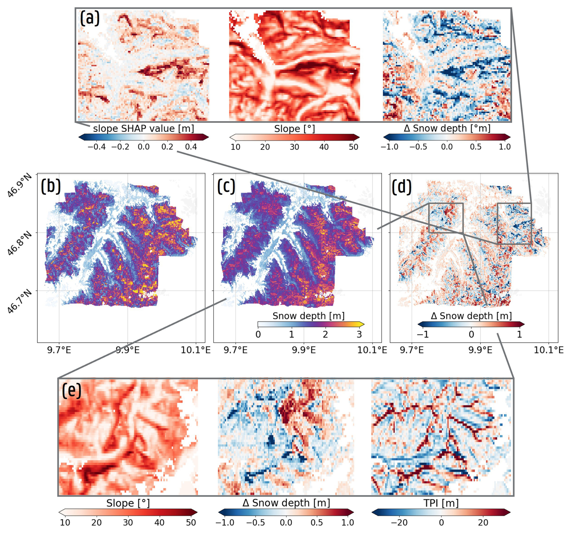
Figure D1 Improvements obtained by adding spatially distributed SD training data (Survey) within the Combination_ML configuration for the 16 March 2017 Dischma valley snow survey. (a) Zoom-in of the difference map (Survey (b) – No survey (c) SD estimates), with corresponding slope and slope SHAP values. The slope SHAP values correspond with the No survey SD estimates. (b) SD estimates from the Combination_ML configuration when no spatially distributed SD data is used during training. (c) Same as (b), but with inclusion of spatial SD training data. (d) Difference map of predicted SD between (b) and (c). (e) Zoom-in of (d), with corresponding slope and TPI values for the area.

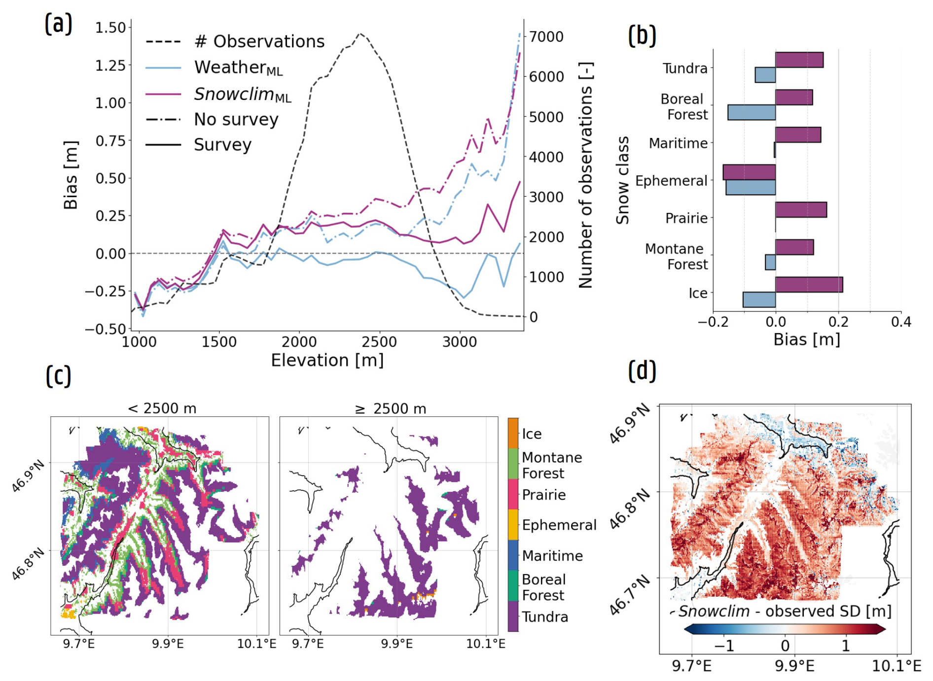
Figure D2 Improvement brought by adding spatially distributed SD training data (Survey) within the Weather_ML and Snowclim_ML configurations for the 16 March 2017 Dischma valley snow survey. (a) Bias for the two configurations within elevation bins of 50 m, trained without (No survey) and with (Survey) spatial SD training data. The black curve displays the amount of observations per elevation bin. (b) Bias displayed per Sturm and Liston (2021) snow class. (c) Spatial distribution of the snow classes within different elevation areas. (d) Difference map between Snowclim SD estimates and measured SD. The black lines in (c) and (d) denote the contour line of 1500 m elevation.

Appendix E: Additional tables and figures

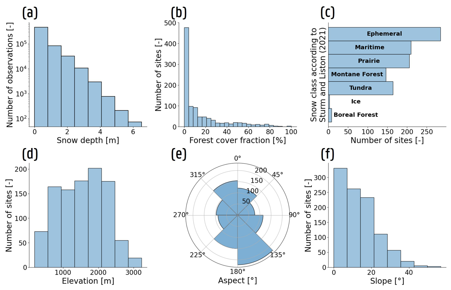
Figure E1 Distributions of measured SD and static features of the in situ measurement sites used to train, validate and test XGBoost. (a) Distribution of measured SD. (b) Distribution of forest cover fraction of the unique measurement sites. (c–f) Same as (b), but for the snow classes described in Sturm and Liston (2021), elevation, aspect and slope, respectively.

Table E1 Overall performance metrics for the PolSAR_ML, Backscatter_ML and Combination_ML configurations for the temporal nested CV framework. The values inside the brackets denote the metric values when zero-measured SD are included in the evaluation.

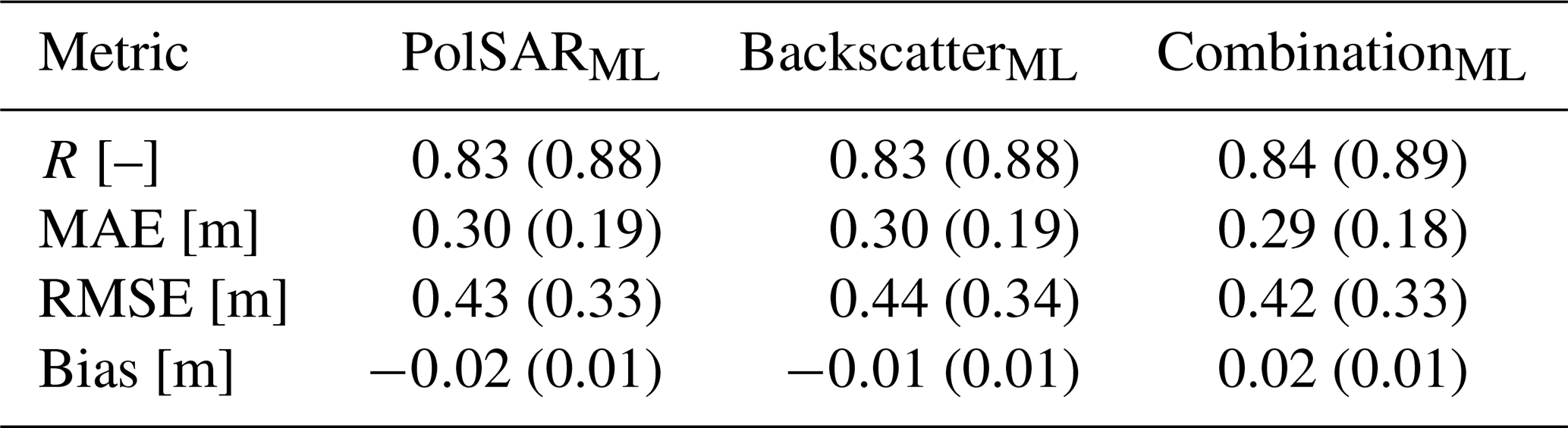
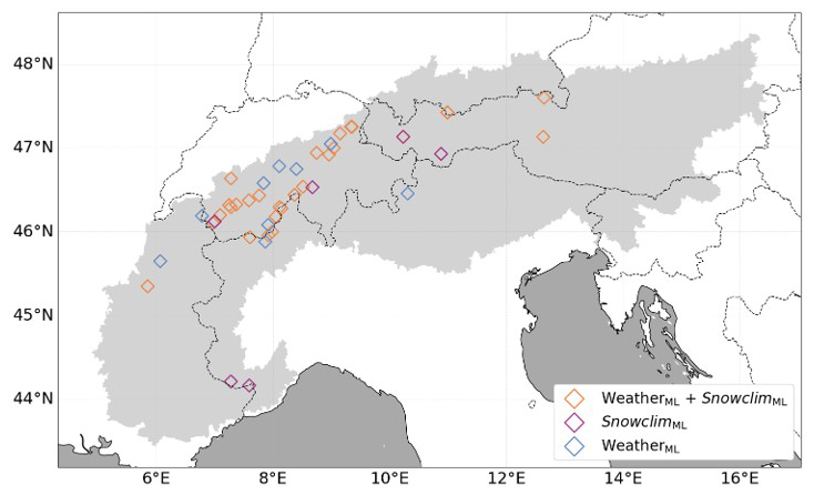
Figure E2 Measurement stations exhibiting a mean site $\text{bias}\le -\mathrm{0.5}$ m within the spatial nested CV framework for the Weather_ML and Snowclim_ML configurations. Sites with fewer than 10 observations are excluded. Colors indicate for which configurations a mean site $\text{bias}\le -\mathrm{0.5}$ m is observed.

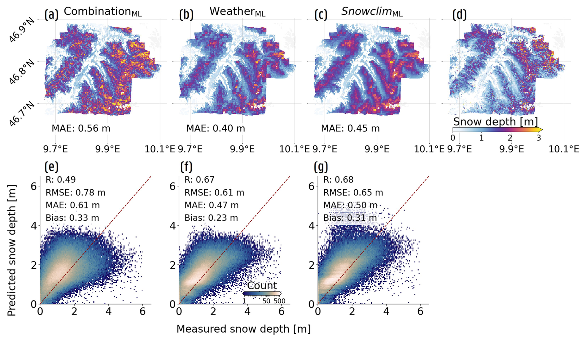
Figure E3 XGBoost spatial prediction performance for the Dischma valley snow surveys with no spatial data included during model training and tuning. The first column (a, e) represents the Combination_ML configuration, while the second and third column show the results for the Weather_ML (b, f) and Snowclim_ML (c, g) configurations, respectively. (a), (b), and (c) display the spatial predictions for the 16 March 2017 snow survey, with (d) representing the measured SD. (e), (f), and (g) show 2D histograms and performance metrics across all nine conducted snow surveys.