Future Retreat of Great Aletsch Glacier and Hintereisferner – application of a full-Stokes model to two valley glaciers in the European Alps

We simulate the future evolution of two valley glaciers in the European Alps over the course of the 21st century. The model setup combines a numerical realization of full-Stokes ice dynamics coupled to a surface energy balance model forced with the sustained (inline with the Paris Agreement) and highest climate emission scenarios based on CMIP5 and CMIP6 data pools. The initialization of the three-dimensional glacier flow model is based on data assimilation, where a detailed observed ice surface velocity map serves as reference for constraining unknown parameters by means of inversion techniques. This setup is applied to Great Aletsch Glacier (GAG) and Hintereisferner (HEF) to assess their individual responses to climate change in the western and eastern European Alps, respectively. The model results of both glaciers are calibrated with comprehensive glaciological observations over several years to ensure a realistic glacier response in the observation period. The end-of-the-century projections reveal a substantial volume loss of both glaciers: HEF is projected to vanish in the middle of the 21st century regardless of the climate emission scenario. GAG is likely to disappear at the end of the 21st century under high-emission scenarios RCP 8.5 and SSP5-8.5, whereas low-emission scenarios RCP 2.6 and SSP1-2.6 predict a median glacier volume reduction of 67.7 % [62.2 % to 77.6 %] and 86.4 % [76.2 % to 89.4 %], respectively (values in brackets correspond to the 17th to 83rd percentile range). Our individual and detailed results of glacier evolution provide well-constrained estimates to complement large-scale modelling efforts. In general, our findings of substantial volume loss at the end of the 21st century align with large-scale modelling outcomes; however, a rough model-intercomparison study reveals a large spread of volume projections with the different glacier models.

1 Introduction

The recent retreat of glaciers is unprecedented at least during the last thousand years (IPCC, 2023), and the glacier mass loss is expected to continue in the 21st century (e.g., Marzeion et al., 2020), maintaining their role as a major contributor to recent sea level rise (Dussaillant et al., 2025; Zemp et al., 2025). Beyond their global impact, glaciers are important for regional water storage and supply, high-alpine ecosystems, hydroelectric power production, tourism and natural hazard regulation in mountain valley regions. Predicting the future development of alpine glaciers is therefore important for various aspects and of high interest for a wide group of stakeholders. In addition to their social and economic importance, glaciers are also one of the most obvious indicators of changes in the climate system. Their geometry responds to variations in atmospheric and climatic conditions through the interaction between surface mass balance and ice dynamics, results in glacier changes related to typical periods of climatic fluctuations. Therefore, the observation and modelling of glacier changes can be used to better understand past, present and future climatic conditions (Pellikka and Rees, 2009).

In view of their enormous importance, there is great interest in accurately simulating glacier evolution over time. Several models for simulating glacier evolution have been developed, ranging from individual glacier applications (Jouvet et al., 2009, 2011; Jouvet and Huss, 2019; Zekollari et al., 2014; Réveillet et al., 2015; Peyaud et al., 2020; Gilbert et al., 2020; Jouvet, 2022; Cook et al., 2023) to regional-scale/global-scale projections (Zekollari et al., 2019, 2024; Hanzer et al., 2018; Maussion et al., 2019; Marzeion et al., 2020; Rounce et al., 2020; Jouvet and Cordonnier, 2023; Rounce et al., 2023; Schuster et al., 2023; Hartl et al., 2025). However, projecting the temporal evolution of glaciers on large spatial scales (global and regional) requires models based on various simplifications, especially with regards to ice dynamics (GloGEM: Huss and Hock (2015), GloGEMflow: Zekollari et al. (2019), PyGEM: Rounce et al. (2020), OGGM: Maussion et al. (2019)). Two of these models (GloGEM, PyGEM) neglects ice flow mass transport and and ice volume projections are based on a retreat parametrization. In the other two models (GloGEMflow, OGGM), ice flow is treated with the Shallow Ice Approximation (SIA), which is computationally efficient but only valid for extensive continuous ice masses (e.g. the interior of ice sheets) with a small aspect ratio (thickness/length). Despite potential shortcomings due to a reduced representation of ice dynamics, large-scale studies of mountain glaciers with such a simplified approach (Zekollari et al., 2019, 2024) suggest a glacier volume loss of 94 %–99 % in Central Europe by the end of the century for the very high-emission scenarios RCP 8.5 (Representative Concentration Pathway, Moss et al., 2010) and SSP5-8.5 (Shared Socioeconomic Pathways Meinshausen et al., 2020). For the low-emission scenarios RCP 2.6 and SSP1-2.6, which are assumed to be in line with the political global warming target of 1.5 °C negotiated in the Paris Agreement (UNFCCC, 2015), an abating volume loss of 63 %–86 % is estimated at the end of the century. The instructured glacier model (IGM,  Jouvet, 2022; Jouvet and Cordonnier, 2023; Cook et al., 2023) emulates Stokes ice flow and is therefore a promising alternative to traditional solvers even on regional scales thanks to its high computational efficiency. However, IGM has not yet been applied to investigate mountain glacier evolution under RCP or SSP climate scenarios. Cook et al. (2023) found that the resulting committed ice loss exceeds a third of the present-day ice volume by 2050.

In turn, detailed ice dynamic studies of individual glaciers often focus on specific applications (e.g., to forecast possible hazards or process understanding), but are also required to assess the impact of simplifications made by large-scale models. Depending on the model complexity, the better representation of physical processes comes with large (or even huge) additional computational costs, which directly transfers into a cumbersome/expensive model tuning and parameter sensitivity evaluation, and even numerical issues (e.g., achieving convergence of a full-Stokes (FS) model is challenging). However, with recent advances in computational resources, solving a FS ice flow model for a complex three-dimensional glacier geometry has become much more affordable. In the hierarchy of ice flow models, the most comprehensive description of ice flow is given by the FS equations (Hindmarsh, 2004) and is most accurate for mountain glaciers with steep slopes and a high aspect ratio (Le Meur et al., 2004). Until now, there has been no clear understanding of whether FS simulations have the ability to narrow uncertainties in current sea-level predictions (IPCC, 2013; Meredith et al., 2019; Oppenheimer et al., 2019). This is a challenging task, since assessing whether FS is needed compared to simpler models is complicated because of many interacting processes (e.g., numerical model used, initialization procedure, design of forward experiments). However, FS models are the most accurate representation of viscous ice flow and, compared to SIA, FS resolves lateral shear stresses and captures the entire stress tensor; for instance, lateral drag by valley glacier sidewalls might be better represented. However, glacier evolution studies under future climate warming scenarios until the end of this century and utilizing a full-Stokes model, or an appropriate higher-order model, are very scarce. A prominent example is Jouvet and Huss (2019), where they estimated a volume loss of the Great Aletsch Glacier (Switzerland) at the end of the 21st century ranging from 60 % (median of full climate forcings) for RCP 2.6 to an almost complete deglaciation for the RCP 8.5 scenario based on a full-Stokes model.

Large uncertainties remain in projections of glacier volume loss on global and regional scales (Marzeion et al., 2020). These uncertainties are not only due to the glacier model used. The choice of the utilized surface mass balance schemes (e.g., temperature index models versus surface energy balance model (e.g., Gabbi et al., 2014), validation of the model response to the type of mass balance observation (glacier-specific vs. regional, Zekollari et al., 2024) or climate data input options (daily vs. monthly resolution (Schuster et al., 2023), downscaling methods and bias corrections of climate data (Weathers et al., 2025)) have a substantial influence on the simulated glacier development. In addition, a common issue of glacier evolution calculations is related to model initialization. This is a well-known problem in glaciology, as illustrated by recent intercomparison experiments focused specifically on the initialization of ice sheet models (Goelzer et al., 2018; Seroussi et al., 2019). While such an intercomparison has not yet been conducted for mountain glaciers, the challenge of initialization remains comparable, as highlighted by Zekollari et al. (2022, Sect. 6 therein). We do not review the different initialization methods, but the three methods discussed in Zekollari et al. (2022) have their own advantages and shortcomings and need to be carefully selected in terms of the research question, model capabilities and performance. In case of sufficiently available data, the most straightforward method consists of starting simulations from an observed state where unknown parameters are constrained by observations. But the initial glacier evolution is often subject to an artificial dynamical shock as the model tends to adjust to the numerical environment and not solely respond, e.g. to the imposed climatic boundary conditions. Usually, an arbitrary relaxation is performed to level out the dynamic shock. Initialization approaches avoiding an artificial dynamical shock come with long spin-up times which are unfeasible for a full-Stokes model and often lack a good agreement of the initialized glacial state with observations (both, ice geometry and ice velocity).

In this paper, our main aim is to perform glacier projections that rely on the most robust physical description on ice flow and surface mass balance calculation. Such a computer-intensive work complement the current research of large-scale glacier volume projections of Central Europe with an individual glacier evolution model based on a higher complexity to investigate the potential variability of glacier responses in the frame of physical process representation. In addition, the framework uses CMIP5 and CMIP6 data Ice dynamics is solved with a full-Stokes model, whereas the coupled surface energy balance model computes the surface mass balance (SMB) on a daily basis. The initialization of the glacier model is based on data assimilation, constraining unknown parameters by an inversion method with respect to observed ice geometry and a large coverage of ice velocities across the glacier. The latter is a common initialization approach for large-scale ice sheet modelling (e.g., Goelzer et al., 2020), but rarely applied for mountain glaciers. The model is applied to two iconic valley glaciers in the Alps with a sufficient data base for the employed ice flow model: (1) the Great Aletsch Glacier (Switzerland) is located in the western Alps and the largest glacier in the Alps with a valley glacier extension. (2) Hintereisferner (Austria) is the largest valley glacier in the eastern Alps and has been classified as one of the ‘reference glaciers’ by the World Glacier Monitoring Service (WGMS). After initialization, we carry out comprehensive model validation to ensure a realistic response of the model in the observation period. Subsequently, ensemble projections are performed for SSP5-8.5, SSP1-2.6, RCP 8.5 and RCP 2.6 to simulate the glacier evolution under different climate scenarios. Finally, these projections are compared to existing large scale experiments.

2 Study sites

This study focusses on two valley glaciers in the European Alps. The Great Aletsch Glacier (GAG, Switzerland, 46.5° N, 8.0° E) is in the western part, while Hintereisferner (HEF, Austria, 46.8° N, 10.8° E) is in the eastern part. An overview of mean annual elevation changes in recent years, selected glacier outlines from the period 1850 until 2015, and the geographical setting is presented in Fig. 1.

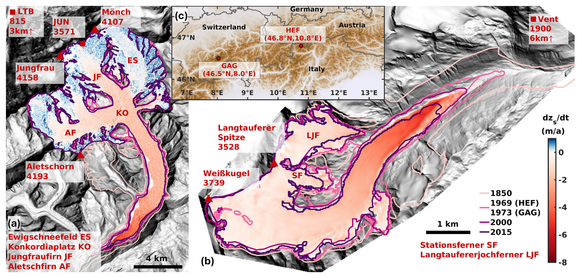
Figure 1 Map of Great Aletsch Glacier (GAG, a) and Hintereisferner (HEF, b) and their location in the European Alps (c). For GAG, mean annual elevation changes, $\partial z_{\mathrm{s}}/\partial t$, are calculated from 2011 and 2019 digital elevation models (DEM,  Leinss and Bernhard, 2021). For HEF, mean annual elevation changes are calculated from 2001 and 2013 DEMs (Sailer et al., 2017; Strasser et al., 2018). Prominent mountain summits are displayed with triangles and meteorological stations with squares. Note that the stations Lauterbrunnen (LTB) and Vent are outside the figure limits. Glacier outlines are taken from the Randolph Glacier Inventory (RGI v7.0) (RGI Consortium, 2023). The hillshade backgrounds are 2011 and 2001 DEMs for GAG and HEF, respectively.

GAG is the largest ice mass in the Alps and originates from the northern main ridge of the Alps. Three main tributaries – Aletschfirn, Jungfraufirn and Ewigschneefeld – join at Konkordiaplatz and form a 15 km long curved tongue that extends to the southwest. The glacier covers an area of 82 km² and the volume of ice amounts to 15 km³, which is about 9.3 % of the volume of the glacier of the Alps, while the elevation ranges from 1600 to 4100 m with ice thicknesses > 900 m at Konkordiaplatz in 1999 (Farinotti et al., 2009). The glacier has been retreating since the Little Ice Age and its volume loss has been estimated to be 4.8 km³ in the period 1880 to 1999, while most of this volume loss has occurred since 1980 (Bauder et al., 2007). The climate at the glacier tongue is relatively dry, but very large amounts of precipitation are measured in the glacier accumulation area, as this area is influenced by precipitation events from the north (Schwarb et al., 2001; MeteoSwiss, 2025).

HEF is a typical valley glacier near the main ridge of the Eastern Alps in Austria. The glacier originally consisted of three main tributary basins. Langtaufererjochferner and Stationsferner were assumed to be disconnected from the main HEF tongue in 1969 and 2000, respectively. However, they are still treated as part of the glacier to maintain consistency in mass balance assessments. The glaciers show one of the longest time series of observations in the Alps (Klug et al., 2018). The accumulation area extends from the Northeast to the Southeast, whereas the long and narrow curved tongue stretches to the Northeast. Weißkugel (3739 m) is the highest point of the HEF, while the terminus of its tongue lies at an elevation of around 2400 m. Ground Penetrating Radar (GPR) surveys in 1997 and 2002 revealed an ice thickness of the tongue exceeding 200 m (Span et al., 2005; Fischer and Kuhn, 2013), while the mean ice thickness in the upper parts of the glacier is less than 100 m. In 2001, the glacier covered an area of 8.25 km² with a glacier volume of 0.57 km³ (Fischer, 2010; Fischer and Kuhn, 2013). Given its area and length, the HEF is among the largest glaciers in the Eastern Alps. Similar to GAG, it exhibits a pronounced valley-glacier extension, which makes it a suitable counterpart for the present comparative study. The HEF is located in the inner dry Alpine zone (Frei and Schär, 1998), which is characterized by very low precipitation compared to the rest of the Alps. The average annual precipitation sum in Vent, about 12 km downstream from HEF at 1900 m a.s.l., reaches less than 700 mm.

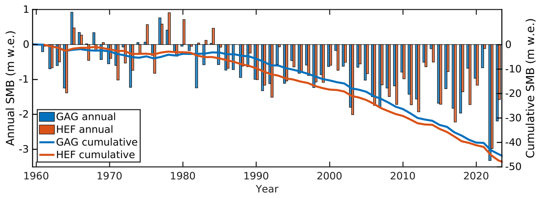
For both glaciers, an exceptional long time series (covering the period from 1960 to present-day) of surface mass balance measurements at stakes over several decades is available (GLAMOS, 2025; WGMS, 2025). Area integrated mass balance terms and spatial distributions are calculated from these measurements with additional data such as snow pit measurements (Huss et al., 2008; Fischer, 2010). Figure 2 shows the annual and cumulative mass balance values for both glaciers. The cumulative mass balance curves reveal a similar behaviour for GAG and HEF. Occasionally, positive years of mass balance occur before 1985. Since then, both glaciers have experienced exclusively negative mass balances, which last until today.

Figure 2 Annual (bars) and cumulative (lines) surface mass balance of GAG (blue) and HEF (red) since 1961 to 2023. Mass balance data are based on GLAMOS (2025) and WGMS (2025) for GAG and HEF, respectively.

3 Climate data

We leverage several datasets to provide a climate forcing to be ready for the projections. Since global circulation model/regional climate model (GCM/RCM) or reanalysis datasets are provided on a coarse resolution and therefore may not cover the local condition of each glacier, we used air temperature and precipitation recordings at meteorological stations to shift the GCM/RCM to a more accurate level. Due to the sparsity of meteorological and GCM/RCM data, we need to make assumptions for downscaling the data to the glacier areas. Therefore, we performed three steps to process the data:

1. Identification of error between ERA5 data and meteorological recordings.

2. Bias adjustment of the projection data to the ERA5 reference data.

3. Downscaling of climate data, either ERA5 or GCM/RCM, to the glacier area.

Step 1: small-scale error: For the period 1961–2023 we used climate variables from the ERA5 reanalysis dataset on a 0.25° spatial and daily temporal resolution (Hersbach et al., 2020). The dataset provides the input variables required for the incoming short- and long-wave radiation, the near-surface air temperature, the surface wind speed, the near-surface specific humidity and the precipitation that are needed to drive the energy balance model (EBM, Sect. 4.3). Note that ERA5 does not provide near-surface specific humidity, but this variable can be computed from dew point temperature and surface pressure (see Appendix A1).

We expect biases of the ERA5 dataset compared to observations at meteorological stations in the vicinity of the individual glacier. Therefore, we applied a simple correction for the near-surface air temperature and precipitation to adjust the ERA5 time series, since other variables are not continuously available. We use direct measurements of near-surface air temperature and precipitation at nearby meteorological stations. For GAG, observed precipitation time series are taken from Lauterbrunnen (815 m a.s.l.) and air temperature from Jungfraujoch (3571 m a.s.l.). Both locations, particularly Lauterbrunnen, are situated at the edge or even at the north of the glacier and might not be fully representative for precipitation sums at the glacier, but we rely on these data because of the absence of a better recording. For HEF, we used the respective time series of temperature and precipitation recorded at the Vent meteorological station (1900 m a.s.l.). The mean annual values of the ERA5 cell closest to the center point of the GAG and HEF is compared with the meteorological station over the period 1961–1990. The period from 1961–1990 is considered as neutral climate period with minor temperature changes (see ERA5 in Fig. 3a) and almost minor cumulative mass balance changes when compared to the period beyond 1990 (see Fig. 2). For the selected ERA5 grid cell (2246 and 2175 m a.s.l. for GAG and HEF, respectively), we use a temperature lapse rate and a precipitation gradient to account for the topographic difference between station and ERA5 data. The inferred bias is used to adjust the GCM/RCM time series of near-surface air temperature and precipitation, respectively.

The bias is estimated by the ERA5 air temperatures, which show an annual mean of −1.40 °C at the point on the grid closest to the reference station in Vent, where an annual mean of 1.85 °C is recorded for our reference period 1961–1990. When accounting for the different elevation levels of ERA5 and the Vent metrological station and a lapse rate of 6.4 °C per 1000 m, the annual mean of ERA5 increases to 0.36 °C. This indicates a cold bias of ERA5 of −1.49 °C compared to the reference station in Vent. We account for this bias by applying a correction value of +1.49 °C. ERA5 precipitation shows a mean annual sum of 1293 mm during our reference period 1961–1990, while at the reference station in Vent only 634 mm were recorded. When accounting for the previously shown elevation difference and a lapse rate of 350 mm per 1000 m, the mean annual sum of ERA5 slightly decreases to 1196 mm. This indicates a considerable wet bias of ERA5 of +89 % compared to the reference station in Vent. We account for this bias by applying a correction factor of 0.53.

A similar correction is performed for the ERA5 data closest to GAG. A temperature bias of +2.16 °C is derived. ERA5 precipitation shows a mean annual sum of  mm during our reference period 1961–1990, while at the reference station in Vent only 633 mm were recorded. When accounting for the previously shown elevation difference and a lapse rate of 350 mm per 1000 m, the mean annual sum of ERA5 slightly decreases to 1196 mm. This indicates a considerable wet bias of ERA5 of +89 % compared to the reference station in Vent. We account for this bias by applying a correction factor of 0.53.

After these corrections, we consider the ERA5 data as appropriate for our modelling study and as a good reference for the bias adjustment applied to the GCM/RCM data (see below). A comparison of the variances of ERA5 and Vent air temperatures shows that also the small scale situation is well captured. Over the entire year, the variance in ERA5 daily air temperatures is 17 % higher than the variance in Vent daily air temperatures. During the ablation season (June–September), where air temperatures are most important for our modelling, the difference is reduced to even less than 4 %. For precipitation, the small-scale situation is less well captured. Although the reference station in Vent shows a mean number of dry days in the accumulation season (October–May) of 136.9, this value is only about a fourth in ERA5 (31.7 d). This matches with the observed wet bias described above. However, as for modelling accumulation the winter precipitation sums are far more important than its daily variability, the applied correction of the wet bias is regarded as sufficient for our modelling purposes.

Although we used a corrected ERA5 time series, we further term the data ERA5. A similar adjustment might be performed with other climate variables, but those are not available at nearby meteorological stations.

Step 2: Bias adjustment: Usually, GCMs and RCMs have systematic biases in their output caused by various factors (e.g. Wood et al., 2004; Maraun, 2016). Therefore, the outputs of global climate models cannot be used directly at local scales to assess the impacts of climate change. Errors or biases are due to limited spatial resolution (large grid sizes), simplified processes and physics, or incomplete understanding of the global climate system. To overcome these biases, a bias adjustment is essential to adjust the statistical properties of the raw GCM/RCM outputs to be consistent with local climate conditions. The time series 1961–2100 of all individual GCM/RCM outputs have been adjusted to the ERA5 grid cell closest to the center point of the GAG and HEF using detrended quantile mapping techniques (DQM) (e.g. Chadwick et al., 2023); note that the ERA5 temperature and precipitation time series have already received a small-scale error adjustment (see above). However, this procedure is similar to Jouvet and Huss (2019), but we use the ERA5 dataset as an observational basis instead of measurements at meteorological stations, since bias adjustment can be performed for the six required variables (which are not or only partially available at the respective metrological stations).

The future projections (2023–2100) are based on two different ensemble datasets: (1) Similar to Zekollari et al. (2019), climate change projections are taken from the EURO-CORDEX ensemble (Jacob et al., 2014; Kotlarski et al., 2014) based on phase 5 of the Coupled Model Intercomparison Project (CMIP5, Taylor et al., 2012). From the entire ensemble, we rely on simulations showing the highest resolution of 0.11° (approx. 12 km horizontal resolution) for the emission scenarios RCP 8.5 and RCP 2.6 and simulations which provide the EBM-relevant climate variables on a daily resolution. This selection corresponds to a total of 65 and 22 simulations for RCP 8.5 and RCP 2.6, respectively, consisting of different combinations of thirteen RCMs, six GCMs and various realizations (see Table S1 and S2 in the Supplement for the selected combinations). (2) As a second data set, we use GCM simulations on a 0.5° (approx. 60 km horizontal resolution) regular grid from phase 3b of the Inter-Sectoral Impact Model Intercomparison Project (ISIMIP3b, Lange, 2019). The chosen ISIMIP3b simulations are based on CMIP6 global climate model simulations (Eyring et al., 2016). We run our ice dynamic simulations for two SSPs: the low-emission scenario SSP1-2.6 and the very high-emission scenario SSP5-8.5. Again, we select simulations from the entire ensemble that provide the required climate variables on a daily resolution (see Table S3 in the Supplement for the selected GCMs). For both scenarios, SSP5-8.5 and SSP1-2.6, ten GCMs are used. A similar dataset has also been employed by Schuster et al. (2023, they use 5 GCMs) using the Open Global Glacier Model (OGGM, Maussion et al., 2019) as a glacier projection tool. Note that ISIMIP3b GCMs are already internally bias-adjusted to W5E5 over the period 1979–2014 (Lange, 2019). However, an additional adjusting of the ISIMIP3b ensemble ensures consistency with the bias adjusted EURO-CORDEX ensemble.

Figure 3 displays the temporal evolution of annual incoming short- and longwave radiation, near-surface air temperature, surface wind speed, near-surface specific humidity, and precipitation change averaged over the Alps for SSP5-8.5, SSP1-2.6, RCP 8.5 and RCP 2.6. The high emission scenarios SSP5-8.5 and RCP 8.5 reveal a mean increase in temperature of approximately 7.8±1.7 and 5.4±1.1 °C by 2100 compared to pre-industrial levels, respectively. The low emission scenarios SSP1-2.6 and RCP 2.6 show a warming of 1.9±0.4 and 2.4±1.1 °C by 2100. As expected, changes in longwave radiation and humidity reveal a similar pattern: The largest increase occurs in SSP5-8.5 followed by RCP 8.5, SSP1-2.6 and RCP 2.6. Changes in precipitation, windspeed, and shortwave radiation are low and not very pronounced.

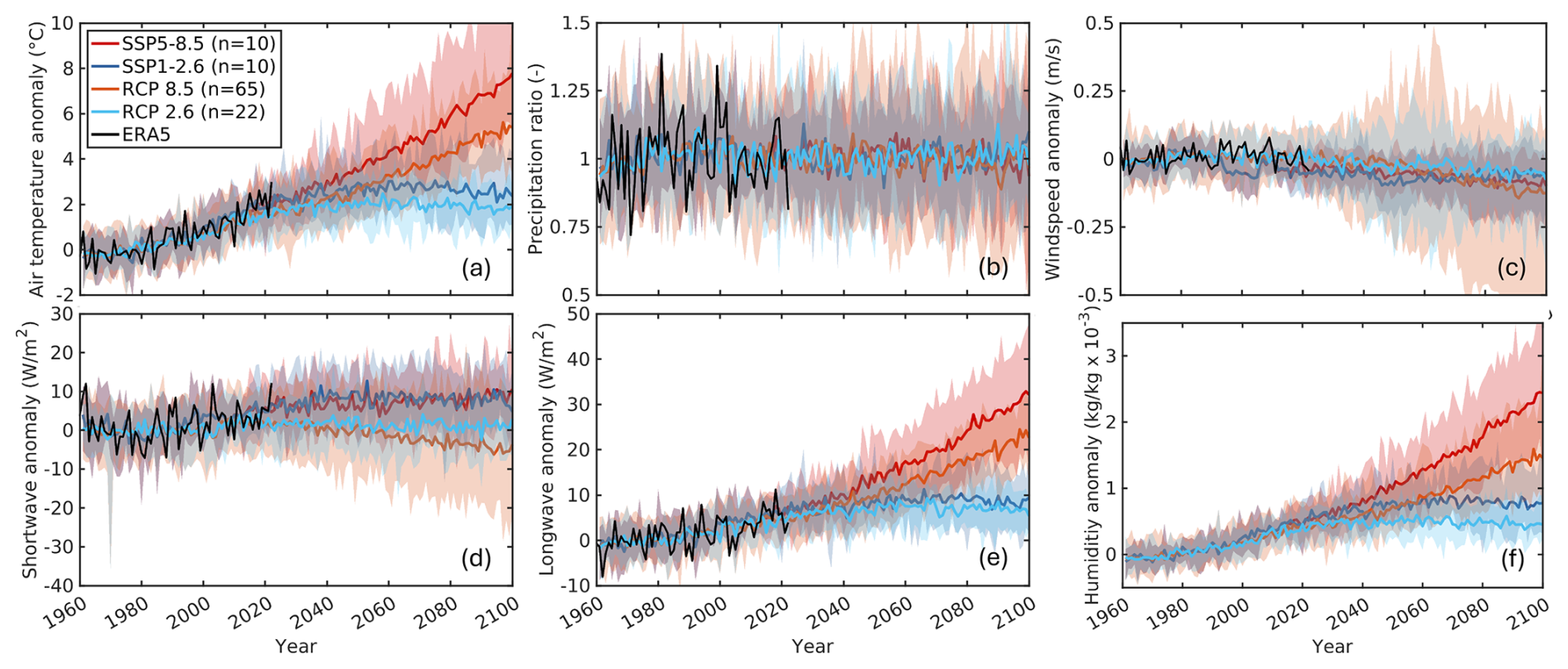
Figure 3 Air temperature (a), precipitation (b), windspeed (c), shortwave radiation (d), longwave radiation (e) and humidity (f) anomalies over the Alps between 1961 and 2100 relative to 1961–1990 of the downscaled GCM/RCM time series of the EURO-CORDEX (RCP scenarios) and ISIMIP3b ensembles (SSP scenarios). The straight lines show the ensemble mean, the lighter background shading covers the area between the ensemble minimum and maximum of each scenario. All variables are additive relative to the reference period, except for precipitation, which is multiplicative.

Step 3: Downscaling: Since the bias adjusted GCM/RCM and ERA5 time series are representative for the elevation at the selected ERA5 grid cell, we apply elevation gradients for downscaling the data to the glacier area. For the near-surface air temperature, a gradient of −6.5 °C km⁻¹ is used (Strasser et al., 2018). Incoming downward long- and short-wave radiation are also assumed to decrease with elevation, showing gradients of −29 W m⁻² km⁻¹ and −13 W m⁻² km⁻¹, respectively (Marty et al., 2002). Precipitation is assumed to increase with elevation, following a gradient of 0.35 m a⁻¹ km⁻¹, which has been used for modelling of the GAG before (Jouvet et al., 2011; Jouvet and Huss, 2019). For windspeed no gradient is applied due to lack of empirical data. We acknowledge that the applied elevation gradients for the different climate variables might not be fully representative for both glaciers, GAG and HEF, but the general lack of related observational data justify this approach. We also intend to use the same gradients to facilitate the comparison of the modelling results.

4 Model description

We employ the Ice-sheet and Sea-level System Model (ISSM; Larour et al., 2012). The applied setup consists of an ice flow component (Sect. 4.1), a glacier evolution component (Sect. 4.2), and a surface mass balance component (Sect. 4.3). All components are combined to simulate the temporal evolution of the glacier.

4.1 Ice dynamics

In the case of glaciers, the Reynolds number is very low (e.g., Fowler and Larson, 1978) and therefore the inertial term in the Navier–Stokes equations can be neglected. This approximation is often referred to as Stokes flow, and the dynamics of the ice flow component is solved with the full-Stokes (FS) equation. The core of the FS equation system builds on the mass balance and momentum equation for incompressible ice and is written as

$$\begin{array}{}\text{(1)}& {\displaystyle }\mathrm{div}\mathit{v}& {\displaystyle }=\mathrm{0},\text{(2)}& {\displaystyle }\mathrm{div}\mathbf{t}& {\displaystyle }={\mathit{\varrho }}_i\mathit{g},\end{array}$$

with the density of ice ϱ_i=917 kg m⁻³, the three-dimensional velocity field $\mathit{v}=(v_x,v_y,v_z)$ in Cartesian coordinates, the gravitational acceleration vector pointing downward $\mathit{g}=-g{\mathit{e}}_z$ (g=9.81 m s⁻²), and the Cauchy stress tensor t. We split the Cauchy stress into a deviatoric part t^D and an isotropic pressure p

$$\begin{array}{}\text{(3)}& \mathbf{t}={\mathbf{t}}^{\mathrm{D}}+p\mathbf{I},\end{array}$$

with $p=-\frac{\mathrm{1}}{\mathrm{3}}\mathrm{tr}\left(\mathbf{t}\right)$ and I the identity tensor. The constitutive equation for the non-Newtonian fluid links the stress tensor to strain rates (i.e., velocity gradients).

$$\begin{array}{}\text{(4)}& {\mathbf{t}}^{\mathrm{D}}=\mathrm{2}\mathit{\eta }\mathbf{D},\end{array}$$

where D is the strain rate tensor ($\mathbf{D}=\frac{\mathrm{1}}{\mathrm{2}}\left(\text{grad}\mathit{v}+(\text{grad}\mathit{v}{)}^T\right)$). The viscosity is given by the Glen-Steinemanns flow law (Glen, 1955; Steinemann, 1954)

$$\begin{array}{}\text{(5)}& \mathit{\eta }={\displaystyle \frac{\mathrm{1}}{\mathrm{2}}}B{\dot{\mathit{\epsilon }}}_{\mathrm{e}}^{(\mathrm{1}-n)/n},\end{array}$$

with the flow law exponent n=3, the ice hardness B, and the effective strain rate ${\dot{\mathit{\epsilon }}}_{\mathrm{e}}$ being the second invariant of the strain-rate tensor. The ice hardness parameter usually covers the temperature dependence of ice deformation and occasional effects like softening due to crevasses. Here, B is inferred by an inversion approach (see Sect. 5.1).

The glacier base is subject to basal sliding according to a friction law for the basal shear stress τ_b in the tangential plane

$$\begin{array}{}\text{(6)}& {\displaystyle }& {\displaystyle }{\mathit{\tau }}_{\mathrm{b}}=-{\mathit{\beta }}^{\mathrm{2}}{\mathit{v}}_{\mathrm{b}},\text{(7)}& {\displaystyle }& {\displaystyle }\mathit{v}\cdot \mathit{n}=\mathrm{0},\end{array}$$

with the unit normal vector n pointing out of the ice, the basal drag parameter β², and v_b is the velocity in the tangential plane at the base. Basal refreezing or melting is neglected. The basal drag parameter for both glaciers is inferred by an inversion approach (see Sect. 5.1). The boundary conditions at the ice base are enforced by Nitsche's method (weak implementation, which reveals better convergence and smoother results than the strong implementation for both glaciers, Cheng et al., 2020).

4.2 Glacier evolution

The glacier surface, $z_{\mathrm{s}}(x,y,t)$, is updated at every time step through the free surface equation (Greve and Blatter, 2009):

$$\begin{array}{}\text{(8)}& {\displaystyle \frac{\partial z_{\mathrm{s}}}{\partial t}}={\mathit{v}}_{\mathrm{s}}\cdot \mathit{n}+{\mathrm{a}}_{\mathrm{s}},\end{array}$$

where $a_{\mathrm{s}}=a_{\mathrm{s}}(x,y,t)$ is the surface mass balance. Assuming an impenetrable glacier bed, z_b, the surface z_s must meet the condition: $z_{\mathrm{s}}-H_{\min }>z_{\mathrm{b}}$. If z_s falls below z_b+H_min the surface height is constrained to z_b+H_min. The minimum ice thickness, H_min, is set to 5 m and ensures numerical stability. We assume that the ice base, z_b, is stationary.

The horizontal extension of the glacier is calculated with a level-set method (LSM, Bondzio et al., 2016), i.e. the glacier front advances horizontally with the ice velocity (no frontal/ice-cliff melt is considered). However, a thickness constraint of H_min = 5 m deactivates/activates elements that fall below/exceed this threshold.

4.3 Surface mass balance

Equation (8) needs a reliable SMB at the glacier surface. Here, we rely on an energy balance model that computes the glacier melt. Snow accumulation, P_s, is calculated from total precipitation, P. The total precipitation is separated into liquid precipitation (rainfall) and solid precipitation (snowfall): Above a temperature threshold of 2 °C precipitation is assumed to be liquid, below 0 °C precipitation is completely solid. We used a smooth cosine interpolation to retrieve the precipitation fraction from solid to liquid between the temperature thresholds of 0 and 2 °C.

For ice melt, we employ the surface energy balance model (EBM) by Evatt et al. (2015). The EBM was originally designed for debris-covered glaciers as it accounts for energy fluxes in a dry porous debris layer on the glacier surface. Both glaciers considered here are mostly debris-free, and therefore the EBM reduces to a clean-ice scheme, where a modulation of the surface heat flux due to a porous supraglacial surface layer is absent. For an exhaustive description, the reader is referred to Evatt et al. (2015). The EBM is forced with the daily near-surface temperature, incoming short- and longwave downward radiation, near-surface windspeed and near-surface specific humidity time series taken from the selected EURO-CORDEX RCMs and the ISIMIP3b GCMs (see Sect. 3). The SMB scheme is run on a daily timestep, but the ice flow model (IFM) is forced with the yearly SMB, as we are interested in the long-term response and not the seasonal variations of the glaciers.

A crucial ingredient for calculating the surface mass balance is the surface albedo α. Here, we use a simple parametrization to calculate the effective albedo which follows the idea of Oerlemans (1992) to make the albedo dependent on the equilibrium line altitude (ELA).

$$\begin{array}{}\text{(9)}& \mathit{\alpha }={\mathit{\alpha }}_{\mathrm{ice}}+({\mathit{\alpha }}_{\mathrm{snow}}-{\mathit{\alpha }}_{\mathrm{ice}})(\mathrm{1}+\tanh (\mathit{\pi }(z_{\mathrm{s}}-\mathrm{ELA}+\mathrm{\Delta })/\mathit{\delta }\left)\right)/\mathrm{2},\end{array}$$

where α_ice is the albedo of bare ice, α_snow is the albedo of snow, Δ a tuneable value, and ELA is the spatially mean ELA of the glacier. The parameter δ ensures a smooth transition from snow to bare ice albedo. Note that the unknown albedo parameters will be tuned to resemble a realistic surface mass balance (SMB) profile over HEF and GAG (see Sect. 5.2). The albedo is updated every year. We also compared our albedo scheme with a more sophisticated albedo parameterization that includes a snow thickness (Oerlemans and Knap, 1998), a temperature-dependent (Slater et al., 1998) or age-dependent snow albedo (Oerlemans and Knap, 1998), but found that the added value is too small given the increase in model complexity and computational cost.

We remain with the same model parameters as in Evatt et al. (2015, Table 1), but climate variables are replaced with the daily time series of the GCM/RCM inputs, and we apply the albedo parametrization (Eq. 9). Note that the thickness of the debris is zero.

4.4 Numerical Model

Numerical solutions of the described ice flow model and related modules are obtained using ISSM. The governing equations are unstable if discretized using the Galerkin finite element method. For the FS equations (Eq. 2), we use condensed MINI elements (Gresho and Sani, 2000) to fulfil the compatibility Ladyzhenskaya-Babuška-Brezzi (LBB) condition (Larour et al., 2012). The computations are run in parallel using the iterative GMRES solver preconditioned using the Additive Schwartz Method (Widlund and Toselli, 2005) with an overlap of 1.

The free surface equation (Eq. 8) is hyperbolic and stabilization is achieved by streamline upwind Petrov–Galerkin diffusion (SUPG, Brooks and Hughes, 1982). We use triangular Lagrange P1 elements (piecewise linear). Similarly, the LSM method is stabilized with SUPG and P1 elements are employed. The reinitialization frequency is set to the ISSM default value of 5. Both equations are solved with GMRES preconditioned with Block Jacobi. However, the numerical handling of the LSM method is studied in detail by Cheng et al. (2024).

The mesh is generated from a regular 2D triangular grid with an edge length of 25 m, and is vertically extruded into five equally spaced layers. This results in a mesh with ≈1.11 million elements for GAG; ≈0.15 million elements for HEF. We ensure that each time step complies with the Courant-Friedrichs-Levy condition (Courant et al., 1928) for numerical stability. Having expected maximum ice velocities of about 200 m a⁻¹ at GAG and 40 m a⁻¹ at HEF we chose a time step of 0.05 and 0.25 years for the masstransport model for the transient simulations, respectively.

Due to the different mesh sizes, the computational demand of the two glaciers is vastly different. For HEF, the future climate runs over 103 simulation years require ≈1.5 h each on 128 cores (2 MPI tasks with each 64 cores). By contrast, a GAG future climate run over 90 simulation years requires ≈ 20 h on 672 cores (7 MPI tasks with each 96 cores). One CPU consists of 2xAMD EPYC 7702 64-Core Processor with 2.0 GHz.

5 Initialization

When simulating glacier temporal evolution, initializing a glacier model is a major challenge that can have a large impact on future projections (e.g., Goelzer et al., 2018; Zekollari et al., 2022). This is a well-known problem and several methods exist which address this problem. All of the proposed methods have their own advantages and drawbacks in order to have an initialized model that resembles both the present-day state and changes of glacier variables (e.g. surface elevation). The choice of the used method is often dependent on the research question, the capability of the model, the availability of observations, or computational resources.

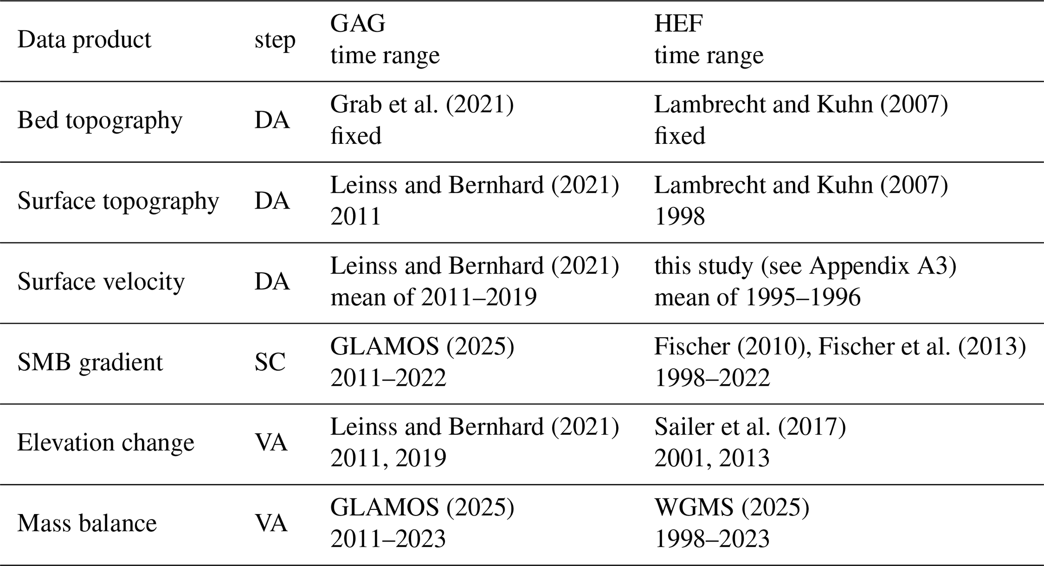
Here, we aim to follow a data assimilation approach: in a first step (DA), the modelled ice surface velocities are inferred to match the observations by means of an inversion technique (Sect. 5.1). In a next step (SC), we calibrate the gradient of the surface mass balance by tuning unknown parameters of the EBM to reproduce observations (Sect. 5.2). In a final step (VA), we run a transient simulation to validate that the transient response matches observations of elevation change and mass balance (Sect. 5.3). Table 1 gives an overview of the data used in the steps described below. Note that the remotely sensed ice surface velocity map of HEF is derived within this work (Appendix A3).

Grab et al. (2021)Lambrecht and Kuhn (2007)Leinss and Bernhard (2021)Lambrecht and Kuhn (2007)Leinss and Bernhard (2021)GLAMOS (2025)Fischer (2010)Fischer et al. (2013)Leinss and Bernhard (2021)Sailer et al. (2017)GLAMOS (2025)WGMS (2025)

Table 1 Overview of the data used in the initialization. Step refers to the step used in the initialization procedure: DA – data assimilation (Sect. 5.1), SC – smb gradient calibration (Sect. 5.2), VA – validation (Sect. 5.3). Time range provides the year(s) used in the respective step.

5.1 Data assimilation

The simulations presented make use of observations for initialization to resemble a certain known state of the glacier. This approach requires the contemporaneity of the products to maintain that, e.g. the ice surface velocity is consistent with the ice geometry. For both glaciers, the required datasets are available (see Table 1) and are bi-linear interpolated on the 25 m triangular mesh. The initialization year for GAG is 2011; for HEF it is 1998.

After initializing the geometry with observed data, an inversion approach is used to infer unknown parameters to resemble the ice dynamics. In particular, the basal drag coefficient β in Eq. (6), which cannot be measured directly, is inferred using an inversion method (Morlighem et al., 2010). In addition, the ice hardness factor B (Eq. 5) is unknown. Usually, it is recovered by a thermomechanical coupled model, since B depends on the temperature (Greve and Blatter, 2009). For reasons of ease of calculation, we do not use such a model here and assume a constant rheology during the friction inversion. We initialize B by computing a vertical temperature profile based on the solution provided by Robin (1955). The computed temperature profile is transferred to B using the relation given by Cuffey and Paterson (2010, p. 75). However, we update B by a subsequent inversion of ice hardness (Borstad et al., 2013) that uses the inferred friction coefficient. The inferred rheology remains unchanged in the projections.

Both inversions minimize a cost function that measures the misfit between observed horizontal velocities and modelled horizontal velocities $\left(v=\sqrt{v_{\mathrm{x}}^{\mathrm{2}}+v_{\mathrm{y}}^{\mathrm{2}}}\right)$ (Morlighem et al., 2010, 2013). Observed horizontal surface velocities are available for both glaciers with large coverage (Table 1). The cost function is defined as follows:

$$\begin{array}{}\text{(10)}& \begin{array}{rl}J(\mathit{v},\mathit{\beta })& =J_{\mathrm{0}}+J_{\mathrm{reg}}=\mathit{\gamma }{\displaystyle \frac{\mathrm{1}}{\mathrm{2}}}\underset{{\mathrm{\Gamma }}_{\mathrm{s}}}{\int }\log {\left({\displaystyle \frac{\sqrt{v_{\mathrm{x}}^{\mathrm{2}}+v_{\mathrm{y}}^{\mathrm{2}}}+{\mathit{\epsilon }}_v}{\sqrt{{v_{\mathrm{x},\mathrm{obs}}}^{\mathrm{2}}+{v_{\mathrm{y},\mathrm{obs}}}^{\mathrm{2}}}+{\mathit{\epsilon }}_v}}\right)}^{\mathrm{2}}\\ & d{\mathrm{\Gamma }}_{\mathrm{s}}+{\mathit{\gamma }}_t{\displaystyle \frac{\mathrm{1}}{\mathrm{2}}}\underset{{\mathrm{\Gamma }}_{\mathrm{b}}}{\int }\mathrm{\nabla }\left(\mathit{\beta }\right)\cdot \mathrm{\nabla }\left(\mathit{\beta }\right)d{\mathrm{\Gamma }}_{\mathrm{b}},\end{array}\end{array}$$

where Γ_s and Γ_b are the ice surface and ice base, respectively. The cost function consists of one term that fits the velocities (J₀). The second term (J_reg) is a Tikhonov regularization to avoid oscillations. The parameters γ and γ_t weight the contributions to the cost function. Following Wolovick et al. (2023), γ and γ_t are defined as follows:

$$\begin{array}{}\text{(11)}& {\displaystyle }\mathit{\gamma }=& {\displaystyle }\mathrm{var}\left(\log \right(\left|v_{\mathrm{obs}}\right|\left)\right)A,\text{(12)}& {\displaystyle }{\mathit{\gamma }}_t=& {\displaystyle }\mathit{\lambda }{\displaystyle \frac{\mathrm{1}}{\mathrm{2}}}\left({\displaystyle \frac{\mathit{\pi }{\mathit{\sigma }}_{(k\text{ or }B})}{\stackrel{\mathrm{‾}}{H}}}\right)A,\end{array}$$

where A is the area of the ice domain, $\stackrel{\mathrm{‾}}{H}$ is the mean ice thickness, and σ_(k or B) is the standard deviation of the initial guess of k or B, and λ is a dimensionless Tikhonov regularization parameter.

We determine the optimal regularization parameter value λ using an L-curve analysis for both inversions. The L-curve is a log-log plot of the smoothness of the optimized variable, indicated by the term J_reg, and the mismatch between the model and the observations represented by the term J₀. For L-curve analysis of the friction inversion, we sample the range ${\mathrm{10}}^{-\mathrm{2}}\le \mathit{\lambda }\le {\mathrm{10}}^{\mathrm{3}}$ with 21 logarithmically spaced samples. For the analysis of the L-curve inversion of ice hardness, we sample the range ${\mathrm{10}}^{-\mathrm{3}}\le \mathit{\lambda }\le {\mathrm{10}}^{\mathrm{3}}$ with 16 logarithmically spaced samples. For each sample, we run the inverse model to convergence and record each contribution to J. The results of the analysis of the L-curve of each glacier are shown in Fig. A1. All L-curves provide a suitable monotony for picking an optimised trade-off value of λ, although not all L-curves show a clear corner. However, for GAG, the selected lambda value of the L-curve analysis of the basal friction is λ=3.16 and λ=0.25 for the inversion of B; for HEF it is λ=0.18 and λ=1.58, respectively.

The final results of the inferred ice flow are presented in Fig. 4. For both glaciers, the observed surface velocity is reproduced with great fidelity (Figs. 4c, d and S2 in the Supplement); we obtain a root mean square error (RMSE) of 1.27 m a⁻¹ for GAG and an RMSE of 0.36 m a⁻¹ for HEF. The maximum ice surface velocity from this analysis at GAG is around 200 m a⁻¹ at a steep ice fall of ES. HEF reaches maximum ice velocities of about 30 m a⁻¹ in the accumulation area, close to the equilibrium line.

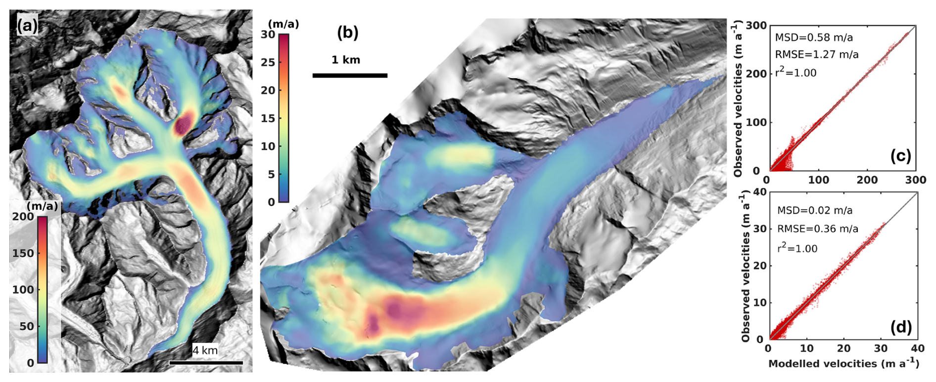
Figure 4 Inferred surface velocity field of GAG (a) and HEF (b) with the corresponding scatter plots in comparison with the observations (c, d) demonstrating the quality of the inversion, respectively.

After inversion simulations, an artificial relaxation run is performed to avoid spurious noise and to allow the model to adjust to its boundary conditions. The primary aim of the relaxation run is to level out the so called dynamical shock but we also intend to preserve the glacial state (surface elevation and ice velocities) of the simulation start date. We experimented with the length of the relaxation period and with the SMB forcing. We found that a relaxation time of ten years and an average SMB forcing from the time period 1952 to 2000 showed that both glacier's glacier volume do not deviate much from the literature values at this time. After relaxation, the glacier volume of GAG and HEF is 12.7 and 0.57 km³, respectively (corresponding literature (extrapolated) values are approx 14 and 0.57 km³, respectively).

5.2 Calibration of the surface mass balance profile

The surface mass balance profile is well known from observations over the last decades for both glaciers. Therefore, we tune unconstrained parameters in the albedo scheme to resemble a valid surface mass balance profile. We sample ranges of parameters in the albedo equation (Eq. 9) ${\mathit{\alpha }}_{\mathrm{snow}}=\mathit{\{}\mathrm{0.7},\mathrm{0.75},\mathrm{0.8},\mathrm{0.85},\mathrm{0.9}\mathit{\}}$, ${\mathit{\alpha }}_{\mathrm{ice}}=\mathit{\{}\mathrm{0.1},\mathrm{0.2},\mathrm{0.3},\mathrm{0.4},\mathrm{0.5}\mathit{\}}$, $\mathrm{\Delta }=\mathit{\{}\mathrm{300},\mathrm{400},\mathrm{500},\mathrm{600},\mathrm{700}\mathit{\}}$ m, and $\mathit{\delta }=\mathit{\{}\mathrm{1500},\mathrm{1750},\mathrm{2000},\mathrm{2250},\mathrm{2500}\mathit{\}}$ m and compare the mean modelled and mean observed SMB profiles over the periods 2001–2013 for HEF and 2011–2019 for GAG. Note, that we compare the mean over the period and not each individual year as we are interested in the long-term behaviour. The comparison periods correspond to the times of available elevation changes (Table 1). The parameters finally selected to result in a satisfying RMSE and mean signed difference (MSD) for HEF are α_snow=0.8, α_ice=0.1, Δ=700 m, and δ=1500 m; for GAG α_snow=0.9, α_ice=0.2, Δ=600 m, and δ=2000 m. The results of the optimized elevation-dependent SMB for both glaciers are shown in Fig. 5b and d and a map view in Figs. 6 and S3 in the Supplement. In order to demonstrate that the tuned values are valid for another climatic period, we re-run the EBM with a mean climate for the neutral climate period 1961–1990 (Fig. 5a and c). For both glaciers, the SMB profile shows a similar good agreement to that period. Note that the 1961–1990 SMB calculations make use of the 2011 and 1998 geometry for GAG and HEF, respectively. However, a general feature observed is that the modelled SMB does not represent the SMB inversion in the upper (accumulation) part of the glacier, which is likely a result of snow redistribution due to wind and avalanches; such processes are not included in our EBM (see Sect. 7.2).

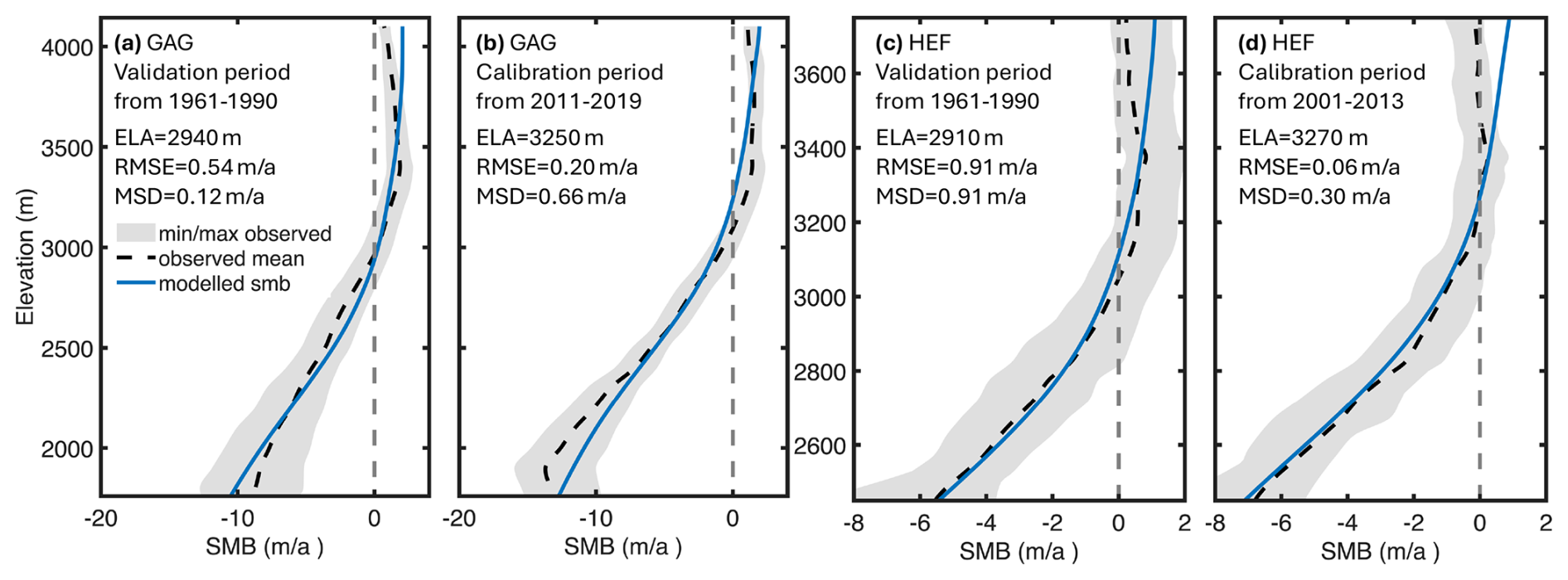
Figure 5 Yearly averaged SMB profiles (blue line) for different periods as computed by the EBM compared to observed SMB profiles (black dashed line). The grey shading shows the observed minimum and maximum of the respective period. (a, b) Computed SMB profiles for GAG for the period 1961–1990 (a) and 2011–2019 (b). (c, d) Computed SMB profiles for HEF for the period 1961–1990 (c) and 2001–2013 (d). Note the different scales of the x- and y-axis for HEF and GAG, respectively.

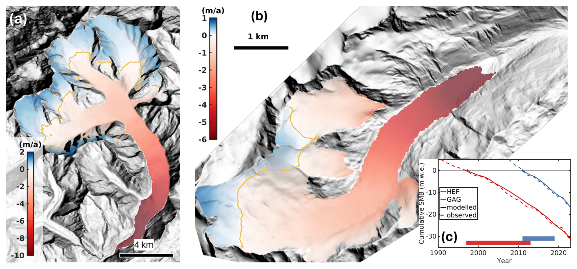
Figure 6 Map view of the mean SMB at GAG for the period 2011–2019 (a) and the mean SMB at HEF for the period 2001–2013 (b). The yellow line in (a) and (b) depicts the location of the modelled ELA (see Fig. 5). The inset (c) shows the temporal evolution of the cumulative SMB compared to the observations with respect to the start time of the simulations (coloured dot). The coloured bars indicate the time period used for smb calibration.

5.3 Validation of glacier evolution until 2023

Based on model initialization and SMB calibration, we run the model forward in time during the period where observations of elevation changes and glacier mass balance of both glaciers exist. Climate data is taken from ERA5, and the corresponding simulation will be termed the ERA5 reference simulation. For GAG, simulation starts at the initial time of 2011 and lasts until 2023; for HEF the start time is 1998 and extends until 2023. Although we put much effort in matching available observations by the initialization and calibration approach, a non-physical dynamical shock at the beginning of the simulation can still occur due to a possible imbalance of the ice mass flux and the SMB. This is often a numerical issue due to, e.g., numerical discretization and diffusion or unresolved processes in the IFM. In order to justify that the model is reasonably initialized for the projections, the modelled elevation changes and cumulative SMB in the observation period are compared to the respective observations. For GAG, the comparison period extends from 2011 to 2019; for HEF from 2001 to 2013 (Table 1). This approach also ensures that independent model fields are used for model tuning (SMB profiles, ice velocity) and validation (long-term cumulative SMB, elevation change). Note that SMB profiles and long-term cumulative SMB are not fully independent, but we want to stress that the long term MB is matched by tuning an average SMB profile.

Modelled elevation changes are shown in Fig. 7 and the respective cumulative mass balance during the simulation periods in Fig. 6c. The modelled cumulative mass balance reveals reasonably good agreement with the observations. Despite the minor variability of the observed cumulative mass balance, the overall decreasing trend is well reproduced by the model of both glaciers. However, the modelled spatial elevation change (Fig. 7) reveals patterns that do not match perfectly with the observed maps (Figs. 1a and S4 in the Supplement). At GAG, glacier thinning seems to extend too far into the upper parts (particularly at ES). At HEF, the modelled elevation change shows localized spots with glacier thickening in the upper part that are not observed (Fig. 1b). Overall, the agreement is rather satisfying, represented by reasonable RMSE (RMSE = 0.98 and 0.57 m a⁻¹ for GAG and HEF, respectively).

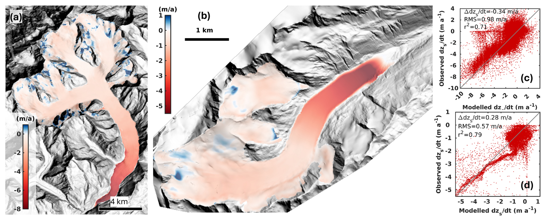
Figure 7 Modelled annual elevation change at GAG for the period 2011–2019 (a) and at HEF for the period 2001–2013 (b). The scatter plots show observed vs. modelled elevation change for GAG (c) and HEF (d).

6 Glacier evolution in the 21st century

Ensembles have been simulated for GAG and HEF for the RCM/GCM models described in Sect. 3. For ensemble statistics we report a multi-model median followed by a likely range defined as the 17th to 83rd percentile range to quantify the uncertainty, unless stated differently in the text.

6.1 Hintereisferner

Figure 8a and b displays the simulation results for HEF's glacier volume in the 21st century, including the median, the 17th-83rd percentile range and the total range for the SSP and RCP scenarios and the ERA5 reference simulation (Sect. 5.3). All climate scenarios show continued ice loss with a substantial loss of glacier volume at the end of the century. The median reduction in glacier volume is 99.7 % with a likely range of 97 % to 100 % at the end of the century among all scenarios.

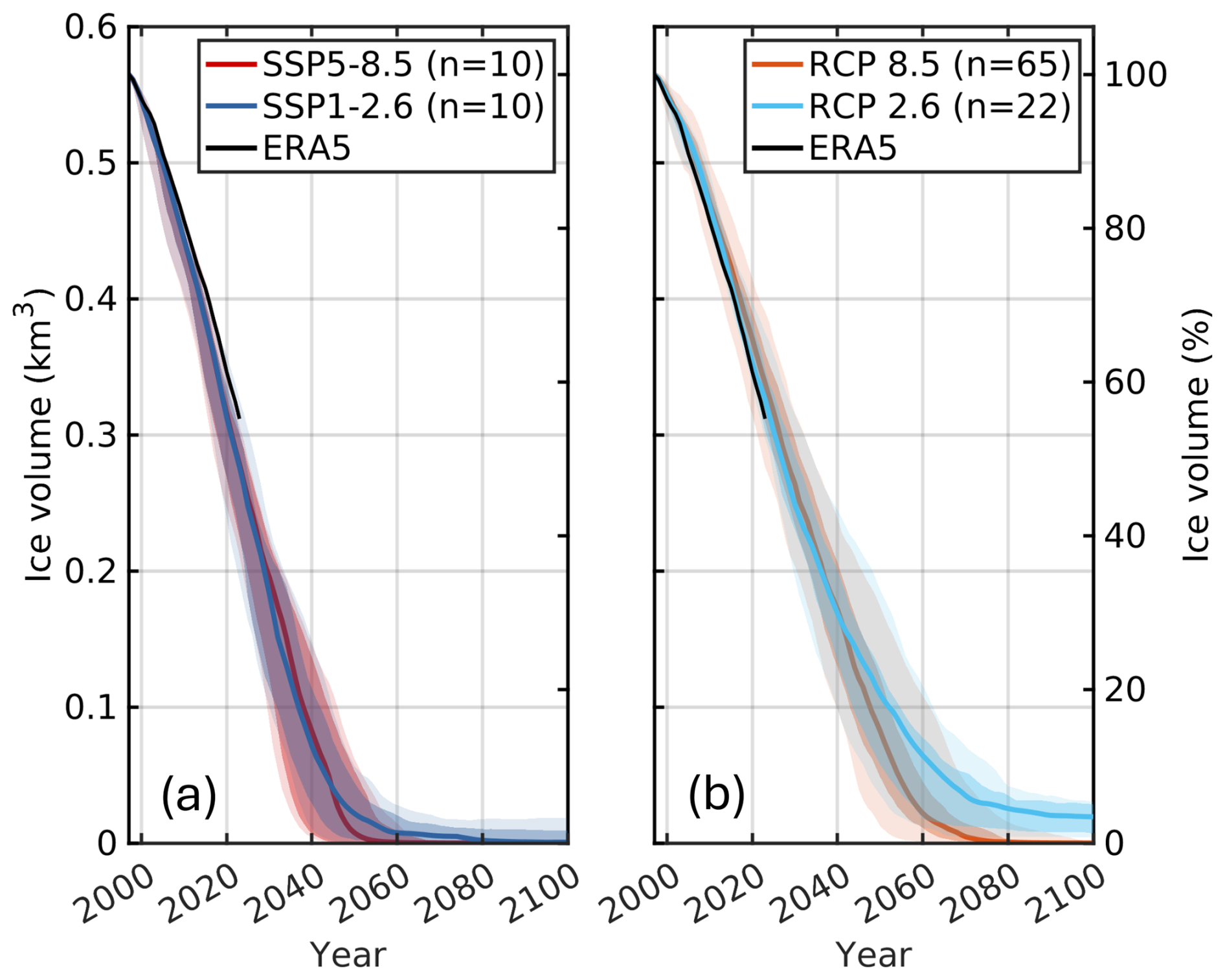
Figure 8 Glacier volume projections of HEF for CMIP6 scenarios' SSP5-8.5 and SSP1-2.6 (a) and the CMIP5 scenarios RCP 8.5 and RCP 2.6 (b). Percentage values are relative to 1997. In addition an glacier volume projection based on the ERA5 reanalysis is shown to demonstrate the scenarios agreement over the past period (see Sect. 5.3). The ensemble median (thick lines), the 17th–83rd percentiles (dark shaded areas) and total range (light shaded areas) is shown.

According to the ensemble median, HEFs ice volume disappears completely in the RCP 8.5 and both SSP scenarios by the end of the century; for the RCP 2.6 an glacier volume of 0.019 km² with a likely range of 0.028 and 0.007 km² remains. In general, the evolution of glacier volume is very similar between each scenario. At the beginning of the century, the SSPs show a somewhat stronger decline in glacier volume than in the RCP scenarios. RCP 2.6 diverges from the other scenarios around 2045 with a somewhat lower volume decrease and a tendency to stabilize around 2080.

We define a completely disappeared glacier (“gone”) as the year in which less than 1 % of the initial glacier volume is left (see Table 2); a “mostly gone” glacier is defined as the year in which less than 10 % of the initial glacier volume is left. For SSP5-8.5, HEF is gone in 2051 with a likely range of 2041 to 2064. Under the SSP1-2.6 pathway, HEF disappeared in 2068 [2047 and beyond 2100]. The RCP 8.5 projects a complete disappearance in 2070 [2063 to 2078]. Although the RCP 2.6 scenarios do not project a complete disappearance, the HEF can be considered to be mostly gone, since only 3.4 % [1 % to 5 %] of the 1997 glacier volume remains. See Tables S1–S3 in the Supplement for glacier projections of each GCM/RCM combination.

Table 2 Projected year for each climate scenario when GAG or HEF are gone (i.e. volume drops below 1 % of the initial volume) or mostly gone (i.e. volume drops below 10 % of the initial volume). Values in the brackets show the likely ranges defined as the 17th to 83rd percentiles. GAG's initial volume in 2011 is 12.7 km³; HEF's initial volume in 1997 is 0.57 km³.

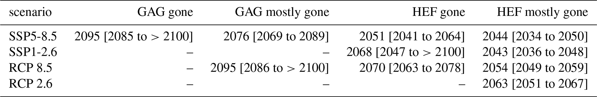
Figure 9a and b display snapshots of glacier area and glacier volume per elevation band of single models that are closest to the ensemble median for the SSP5-8.5 and RCP 2.6 scenarios, respectively. The figures do not show the full range of possible results of the entire ensemble for each scenario and are intended as a general overview. In both scenarios, a complete disintegration of the glacier tongue is expected to occur. Under RCP 2.6 scenarios, ice patches located beneath Weißkugel and Langtaufererjochferner at elevations above approximately 3200 m a.s.l. are projected to persist until the year 2100, although they could potentially disappear after this period. In the mid-century, Langtaufererjochferner and Stationsferner disconnected from the accumulation part of the glacier and become independent ice patches.

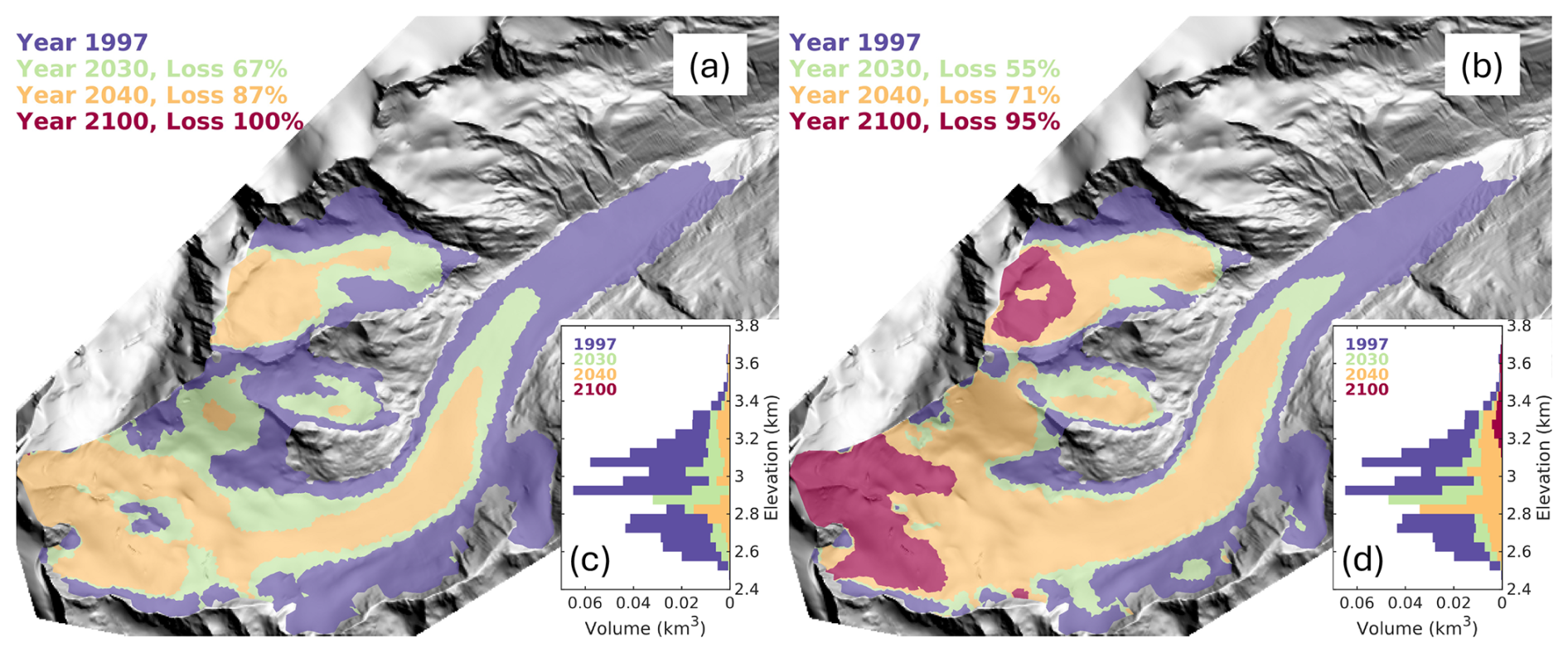
Figure 9 Glacier area of HEF in different years for SSP5-8.5 (a) and RCP 2.6 (b) of a single model which is closest to the ensemble median volume. The percentage values present the glacier volume loss of the individual years with respect to 1997. Insets (c) and (d) show the distribution of glacier volume per 50 m elevation bands in different years.

6.2 Great Aletsch Glacier

Figure 10 displays the simulation results for GAG’s glacier volume in the 21st century, including the median, the 17th–83rd percentile range and the total range for the SSP and RCP scenarios and the ERA5 reference simulation. Similarly as HEF's glacier volume projection, GAG shows continued ice loss with a substantial loss of the glacier volume at the end of the century.

Figure 10 Glacier volume projections of GAG for CMIP6 scenarios SSP5-8.5 and SSP1-2.6 (a) and the CMIP5 scenarios RCP 8.5 and RCP 2.6 (b). Percentage values are relative to 2011. In addition an glacier volume projection based on the ERA5 reanalysis is shown to demonstrate the scenarios agreement over the past period (see Sect. 5.3). The ensemble median (thick lines), the 17th–83rd percentiles (dark shaded areas) and total range (light shaded areas) is shown.

Until ≈2040, the reduction in glacier volume is almost similar for individual climate scenarios, but diverges afterward. In 2040, the median reduction in glacier volume is approximately 31.4 % [26.8 % to 35.7 %] among all scenarios. The spread of individual climate scenarios in terms of glacier volume is considerable at the end of the century. In 2100, the median reduction in glacier volume is 88.5 % [71.8 % to 97.7 %] among all scenarios. For RCP 2.6 and SSP1-2.6 an glacier volume reduction of 67.7 % [62.2 % to 77.6 %] and 86.4 % [76.2 % to 89.4 %] is expected, respectively. Both low emission scenarios tend to stabilize towards the end of the century above 10 % of the initial glacier volume, but the decline in glacier volume seems to continue after 2100. The high emission scenarios RCP 8.5 and SSP5-8.5 lead to an glacier volume reduction of 92.6 % [87.2 % to 97.7 %] and 99.7 % [96.4 % to 100 %], respectively. The SSP5-8.5 projects a complete deglaciation in 2095 [2085 and beyond 2100] (Table 2). Glacier volumes drop below 10 % in the RCP 8.5 in 2095, which is about 19 years later than in SSP5-8.5 (Table 2). See Tables S4–S6 in the Supplement for glacier projections of each GCM/RCM combination.

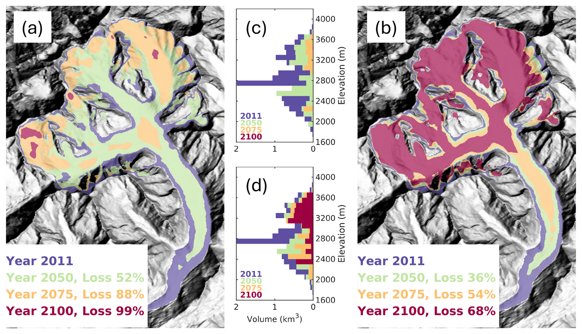
Figure 11 Glacier area of GAG in different years for SSP5-8.5 (a) and RCP 2.6 (b) of a single model which is closest to the ensemble median volume. The percentage values present the glacier volume loss of the individual years with respect to 2011. Insets (c) and (d) show the distribution of glacier volume per 100 m elevation bands in different years.

Figure 11a and b displays snapshots of glacier area and glacier volume per elevation band of single models that are closest to the ensemble median for the SSP5-8.5 and RCP 2.6 scenarios, respectively. These examples, representing the upper and lower extremes, do not encompass the full range of possible results, but are intended to provide an insight of the glacier retreat. In both scenarios, a complete disintegration of the 14 km long glacier tongue is expected to occur. In SSP5-8.5 an almost complete GAG disappearance by 2100 is expected with only tiny ice patches in regions above ≈3400 m a.s.l. persisting until the year 2100 (Fig. 11c). For RCP 2.6 a major retreat of GAG by the end of the century is expected, but Konkordiaplatz is still connected to the three main tributaries Aletschfirn, Jungfraufirn and Ewigschneefeld. Most of the ice remains in the higher parts (Fig. 11d), however some ice is present in the lower-lying regions. The prominent feature is the peak of glacier volume around the 2400 m elevation band in the year 2100. This peak is associated with the Konkordiaplatz site, which initially has a surface elevation of ≈2800 m a.s.l. and an ice thickness exceeding 900 m. As the ice at this location persists but the surface elevation decreases, the initial peak at around 2800 m a.s.l. decreases and shifts to a lower elevation. Although RCP 2.6 is expected to preserve more ice at the end of the simulation period than SSP5-8.5, for example, the landscape will change significantly compared to today.

7 Discussion

7.1 Parameter uncertainty

Our provided projections are based on a calibration strategy for parameters to provide a best-estimate. However, several parameters in the EBM are subject to large uncertainty that is not covered by our best-estimate simulations. For instance, the gradients used for downscaling the incoming short- and longwave radiation are highly uncertain as they are based on one study measured at one location. In order to test the sensitivity of our projections on parameter choice, we use an ad-hoc approach by simply varying uncertain parameters by ±10 %. Although this variation will likely not cover the possible range of parameters, it illustrates model outcomes by the full-Stokes model to parameter changes. The parameter's we change encompasses (i) the downscaling gradients of short- and longwave radiation, precipitation, air-temperature, (ii) the error estimate of precipitation and air-temperature between ERA5 data and meteorological station (iii) and the effective albedo. Simulations of these parameter combinations are re-run for SSP 585 and RCP 26, covering the upper and lower end-members of the climate pathway, with the GCM/RCM combination closest to the ensemble median (See Tables S1–S6 in the Supplement). This results in 14 parameter combinations for each glacier and will be termed the “parameter ensemble”.

Figure 12 shows the computed SMB profiles of the parameter ensemble. For almost all settings, the SMB profile is similar to the “best estimate”. Except for changing the albedo by ±10 % deviate much larger from the “best estimate” but is still, however, within the range of the maximum and minimum range (at least below the ELA). The subsequent projection runs (Fig. 13) of the parameter ensemble reveal that the parameter ensemble has a minor effect on projected glacier volume loss or glacier gone times (considering the median ± percentile range). However, the change in albedo by ±10 % has a larger impact (see the total range of the low emission scenario in Fig. 13).

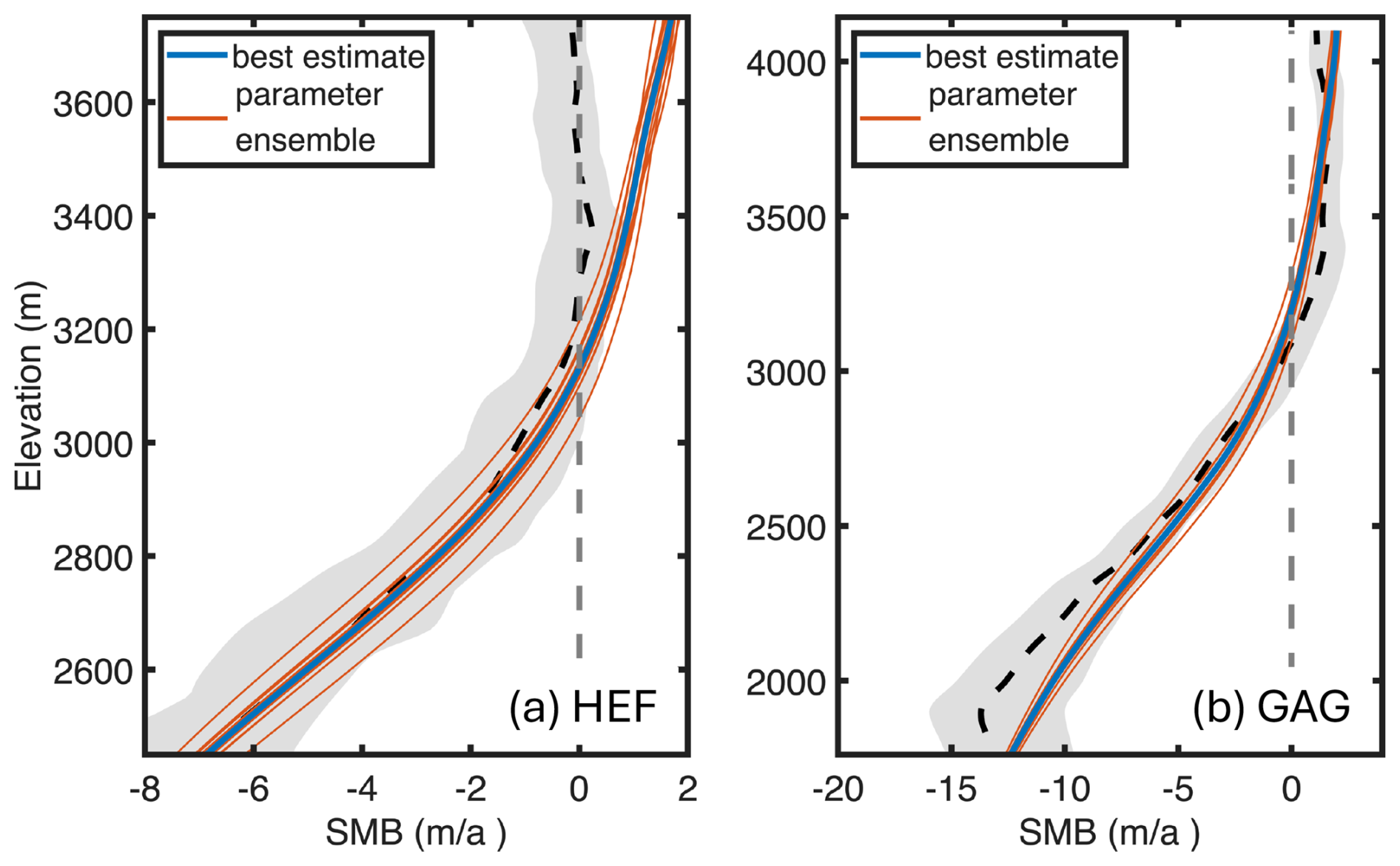
Figure 12 Computed SMB profiles of the parameter ensemble (red lines) compared to the best estimate (blue line, see Fig. 5) for HEF for the period 2001–2013 (a) and GAG for the period 2011–2019 (b). The grey shading shows the observed minimum and maximum and the black dashed line the mean over the respective period. Note the different scales of the x- and y-axis for HEF and GAG, respectively.

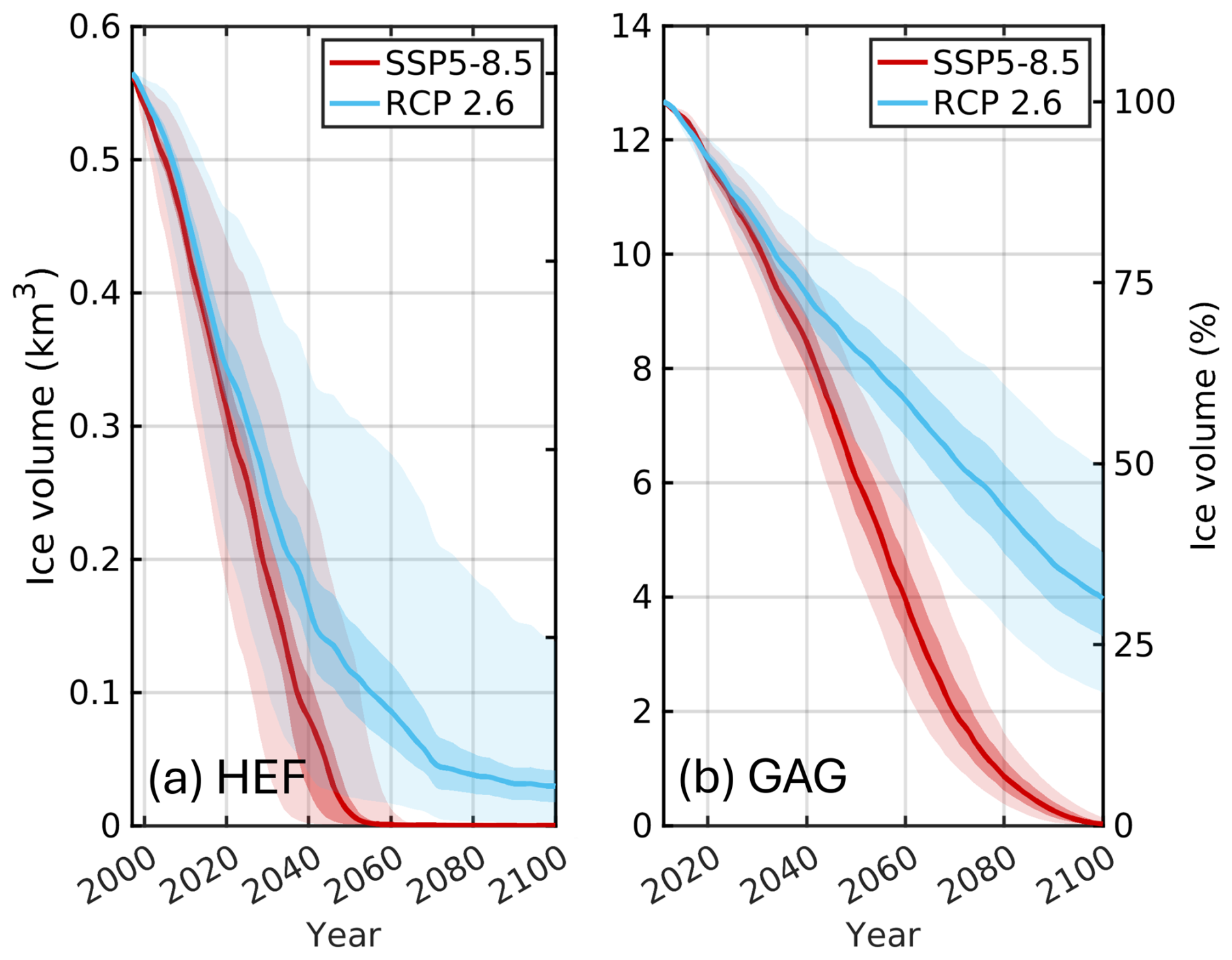
Figure 13 Glacier volume projections of the parameter ensemble for HEF (a) and GAG (b). The ensemble median (thick lines), the 17th–83rd percentiles (dark shaded areas) and total range (light shaded areas) is shown.

7.2 Uncertainties of the model setup

Despite the fact that we use a rather complex model in terms of FS ice dynamics compared to large-scale glacier models relying mainly on SIA (e.g., Zekollari et al., 2019; Schuster et al., 2023) and a more sophisticated SMB model employing a surface energy balance model compared to simpler models (e.g. temperature index models, Schuster et al., 2023), our results are subject to several uncertainties, and some of them we will discuss below.

Our inversion approach makes use of a remotely sensed surface velocity product as a target to constrain unknown parameters. However, the target velocity field itself is affected by uncertainties that are transferred to the IFM. On the one hand, retrieving the velocity of the ice surface of slow flowing glaciers from satellite sensors is challenging and subject to large errors particularly in slow flowing parts (i.e. accumulation zones). The retrieved observed ice flow velocity is subject to methodological errors which leads to an uncertain observed ice velocity map. The transport of ice, particularly in the accumulation area, downstream of the glacier could be subject to this uncertainty. On the other hand, the inferred basal state resulting from the inversion approach remained unchanged during the projection period. The basal friction parameter and thus the basal slipperiness could change during the projection period due to increased availability of meltwater at the base, and therefore decreased overburden ice pressure. These effects are not captured by our model (basal drag is only dependent on velocity (Eq. 6)), and the basal state reflects the initial state. Furthermore, thermo-mechanics are not taken into account, which might have an impact on the overall glacier evolution (Yan et al., 2023).

In addition to the uncertainties related to the IFM, the external forcing data are subject to several uncertainties. We are relying on future climate data from CMIP5 and CMIP6, where each GCM/RCM has its own uncertainty that produces a large spread in glacier projections. For example, in some individual GCM/RCM projections of the GAG, low-emission projections of the glacier volume at 2100 overlap with simulations of high-emission scenarios (compare the full spread of SSP1-2.6 with the full spread of SSP5-8.5 and RCP 8.5 in Fig. 11). The comparison of the overlapping projections is certainly hampered, as they stem from different GCM/RCMs but demonstrate the spread of the projections.

The study by Matiu et al. (2024) reveals the challenges encountered when using climate model data in mountainous environments. The GCM/RCM data used have a rather coarse resolution (between 12 (EURO-CORDEX) and 60 km (ISIMIP3b)) in terms of the length scale of mountain glaciers in the European Alps. Mountainous regions are characterized by complex topography and the local climate is driven mainly by the interaction between large-scale atmospheric flows and local topography. Although the employed downscaling and bias correction ensure a reasonable level of the climate variables, the overall climate output has systematic biases. Small scale variability of atmospheric dynamics, originating from complex air flow modifications by mountainous terrain is not resolved in the rather large-scale resolution GCM data. This might introduce unquantifiable inaccuracies and biases in the climate data and has to be borne in mind, when interpreting the results. A distinctly higher spatial resolution of the climate data would be necessary to adequately represent the relevant physical processes. For instance, for better resolving the turbulent fluxes (latent and sensible), requires a more sophisticated windspeed model accounting for small scale variability. However, this is beyond the scope of this study and computationally way too expensive to be accounted for in the scope of this study given the 107 different climate projections used in the modelling process.

Uncertainties in the calculated SMB are not solely due to climate data; they also arise from potential overestimations in snow accumulation at higher elevations, as we lack a model for snow redistribution by wind transport and avalanches. We experimentally applied a snow redistribution model based on surface slope and curvature following Huss et al. (2008), but it resulted in only minor improvements relative to the validated SMB gradients without incorporating a wind/avalanche redistribution model (see Fig. 5). Moreover, when incorporating snow redistribution based on surface slope and curvature, our model experiences instabilities in the evolution of the ice surface (e.g., holes in the surface). Although the parametrizations of snow redistributions appear promising, further refinement for application in an IFM is required.

The rate of future glacier retreat is certainly affected by supraglacial debris that alters the SMB. A debris cover has many feedbacks on the SMB by decreasing the albedo leading to enhanced melt or due to its insulating properties leading to decreased melt (Østrem, 1959). Although the glacier tongue of GAG is completely protected by a debris cover and Jouvet et al. (2011) demonstrate that a supraglacial debris cover reduces glacier melt, i.e. glacier retreat, we refrain from using such a parametrization. Although they tuned the SMB to observations, Jouvet et al. (2011) used a simplified parametrization for a debris induced SMB that did not account for future supraglacial debris transport, debris redistribution and developing ponds and cryokarst features (Mayer and Licciulli, 2021; Ferguson and Vieli, 2021), which we think is necessary for future projections.

7.3 Comparison with previous results

The future evolution of glaciers in the European Alps has been projected with models of various complexity and based on diverse climate projections. Our results of a substantial volume loss until the end of the 21st century under CMIP5 and CMIP6 future climate scenarios are in line with previous estimates based on large-scale (Zekollari et al., 2019; Schuster et al., 2023) and detailed glacier modelling studies (Jouvet and Huss, 2019) (Fig. 14). However, the timing of deglaciation and the remaining glacier volume at the end of the 21st century vary considerably.

The study by Jouvet and Huss (JH19, 2019) is comparable to our research with respect to the model configuration. They utilize an individual full-Stokes model setup for GAG, with model tuning and validation based on observations (glacier volume and length of glacier tongue, in-situ point measurements of ice surface velocities, and surface mass balance). However, JH19 predicts a larger volume loss by the end of the 21st century relative to our findings. For RCP 8.5, they predict a 98.5 % reduction in glacier volume, while our model predicts a reduction of 92.6 %. Specifically, under RCP 2.6 they predict a 59.5 % reduction in glacier volume, contrasting our model prediction of 67.7 %. The discrepancies may originate from the different models employed for calculating surface glacier melt. Our study utilizes a physically-based energy balance model, while JH19 employs a temperature index model (Hock, 1999; Huss et al., 2008). Although both models tend to overestimate the mass budget and have a limited ability to reproduce glacier volume on decadal time scales, the mass budget computed by an energy balance model, despite its physical character, is probably too high (compare HTI and EB schemes in Gabbi et al., 2014). However, this behaviour is only applicable for the RCP 8.5 scenario and RCP 2.6 until about 2075; afterwards the RCP 2.6 of JH19 reveals declined mass loss.

The volume projections of the large-scale models are generally situated above (GloGEMflow) or, close (OGGM) to our projections. Under RCP 2.6, GloGEMflow predicts a volume reduction of 57.6 % for GAG, aligning somewhat more closely with our forecast than the JH19 study; likewise, for RCP 8.5, GloGEMflow projects a 89.4 % volume decline, which is closer to our estimate than the JH19 study. OGGM displays an irregular pattern when compared to our projections. Under the SSP5-8.5 scenario, discrepancies are pronounced in the mid-century period but diminish significantly after 2075. Conversely, for the SSP1-2.6 scenario, the differences remain minor before 2075, although OGGM projects glacier growth in the subsequent years. In the case of HEF, the OGGM model aligns well with our projections over the entire projection period for the SSP5-8.5 and SSP1-2.6 scenarios. In contrast, GloGEMflow exhibits significant discrepancies. Although GloGEMflow predicts an almost complete disappearance of GAG by the end of the century, the projected volume loss is significantly delayed (≈50 years) compared to OGGM and our study. Under the RCP 2.6 scenario, a substantial proportion of ice remains (32.5 %) compared to OGGM and our study. In line with the JH19 experiments, there is no clear trend whether a TI and EBM model predicts more mass loss or not.

Disentangling the reasons for the differences is challenging, particularly when comparing model projection outcomes based on large-scale approaches to individual glacier applications, since model techniques are designed in a different manner. In addition to inherent differences arising from model concepts and design, other contributing factors include the climate forcing datasets used, the methodologies of model calibration and initialization, as well as the choice of the mass balance schemes. Please note that the comparison of the selected studies aims to demonstrate the possible spread of the model outcomes, but is not fully exhaustive, as we did not include additional studies that present projections of GAG and/or HEF (e.g., Hanzer et al., 2018; Zekollari et al., 2024; Hartl et al., 2025). However, our selective comparison demonstrates the potential spread of glacier model projections with regard to model sophistication, initialisation and forcing.

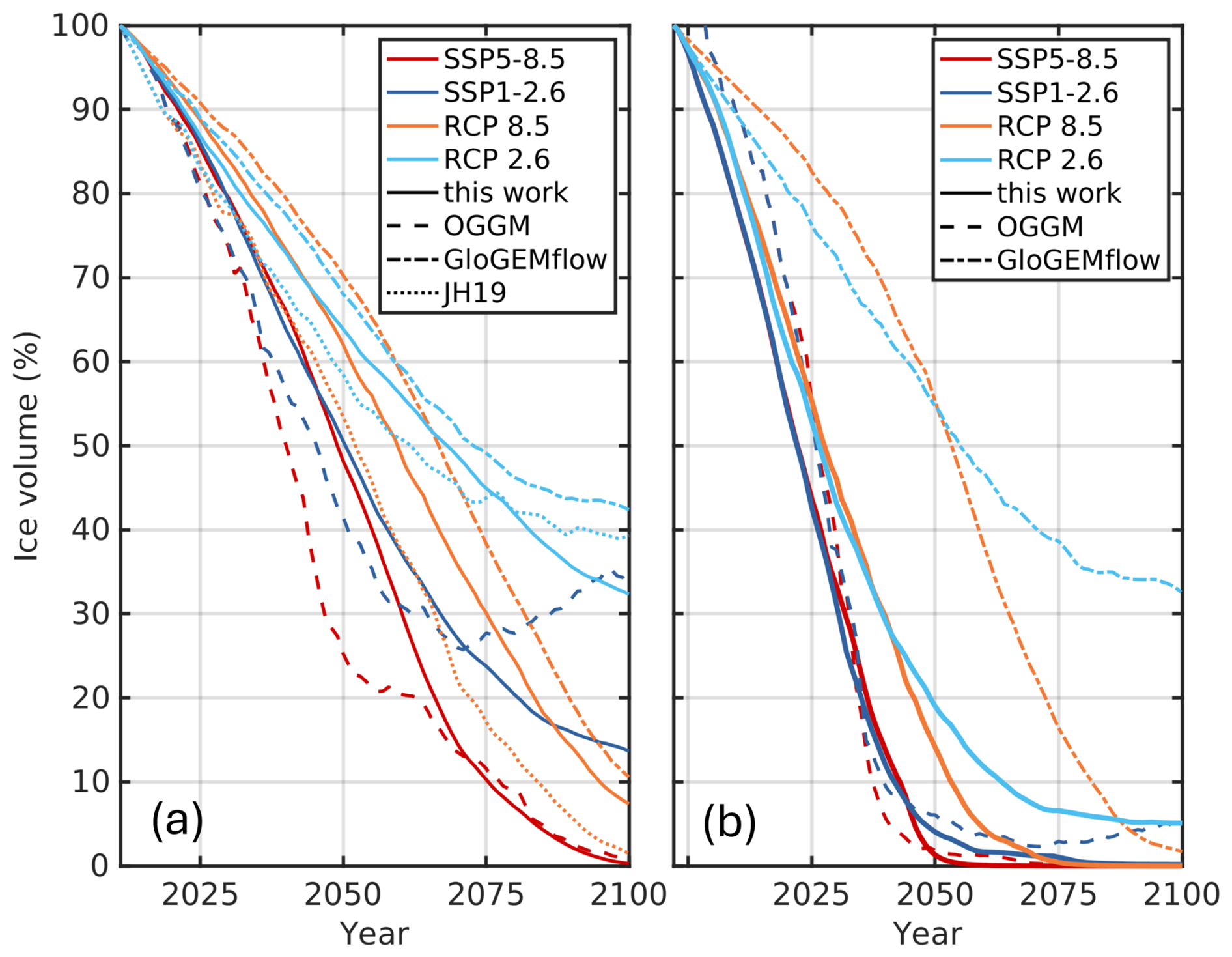
Figure 14 Comparison of glacier volume evolutions from previous studies for GAG (a) and HEF (b). Results of the large-scale models OGGM and GloGEMflow are from Schuster et al. (2023) and Zekollari et al. (2019), respectively. JH19 refers to the detailed full-Stokes study of GAG by Jouvet and Huss (2019). For each study, the ensemble medians are shown with the exception of GloGEMflow, for which the ensemble mean is presented. Note, that the projection start date of GloGEMflow is 2017 and we use a linear extrapolation to 1997.

7.4 Generalization

The most striking feature of the volume projections is that even in low emission scenarios, the HEF (almost) disappeared. In addition, the low- and high-emission scenarios at HEF are rather identical in terms of glacier volume loss. The losses agree pretty well with the expectation of (almost) full deglaciation of HEF in the middle of the 21st century. This is an intriguing result, since limiting global warming to 1.5 to 2 °C above pre-industrial levels negotiated within the Paris Agreement would cause a (almost) complete disappearance of HEF, regardless of whether the sustainable or the highest emission pathway is considered.

GAG has a longer lifetime than HEF in the different future climate scenarios. While GAG is projected to disappear under high-emission scenarios, low-emission scenarios suggest the need for stringent mitigation measures to prevent further reduction of GAG's glacier volume. The longer lifetime of GAG is related to its larger ice thicknesses that persist even at low altitude (Fig. 11c, d), its larger elevation range and its higher elevation-area distribution. Figure 15a and b show the distribution of glacier area per elevation bands of GAG and HEF and the evolution of the ensemble-median ELA of each scenario. Notable is the increase of the ELA at HEF for each scenario reaching, or even exceeding, the ice coverage fraction at the highest elevation; merely the ELA under RCP 2.6 forcing reaches a height that is below a certain fraction of the present-day ice coverage. At GAG, the increase of the ELA for the low-emission scenarios is muted compared to the high-emission scenarios. In particular, a large fraction of glacier area above >3500 m a.s.l. would remain.

The examined sample is certainly not representative for all glaciers in the alps, but simply upscaling our projection results of HEF and GAG to all glaciers in the European Alps would cause an almost complete wastage of glaciers in the eastern Alps, while a tiny fraction in the western Alps is expected to survive (Fig. 15c). This estimate is supported by Hartl et al. (2025), where all warming-level scenarios lead to a nearly complete deglaciation in the Ötztal and Stubai Alps (western Austria) before 2100. In the western alps, glaciers covering an elevation range above ≈3500 m a.s.l. have a longer lifetime or even the potential to survive until 2100. However, in the worst scenarios, we extrapolate that most glaciers in the western alps disappear at the end of the 21st century, which is consistent with Van Tricht et al. (2025).

The simple extrapolation of two exemplary glaciers to all glaciers in the European Alps is certainly hampered by several factors. In addition to the regional setting of each glacier that probably influences the glaciers' response to increasing temperatures, the glacier sensitivity depends on glacier slope and exposition, ice thickness and area-elevation distribution, mass balance gradient and hypsometry (e.g. Oerlemans, 1992; Jiskoot et al., 2009). However, comparing the regional settings GAG receives very high amounts of precipitation in the accumulation area due to moist air masses from the north. However, these air masses are blocked by the main alpine crest and create very dry conditions in the inner-Alpine valleys (e.g., Rhone valley), which leads to considerably smaller amounts of precipitation at GAG's glacier tongue.

HEF, as well as other low-lying glaciers found in the eastern European Alps, are particularly vulnerable to increasing temperatures because they are situated at lower elevations than many of their western counterparts (Fig. 15c), which reside at higher altitudes. In addition, HEF experiences a somewhat more intense warming than GAG. For RCP 8.5 a stronger warming of 0.7 ± 0.9 °C is expected at HEF compared to GAG; for RCP 2.6, SSP5-8.5 and SSP1-2.6 0.3±0.6, 0.2 ± 0.2, and 0.3 ± 0.2 °C, respectively. Note that the estimated values correspond to an elevation of ≈2200 m a.s.l. beneath GAG and HEF, but temperature changes are subject to local conditions and elevation (Matiu et al., 2024).

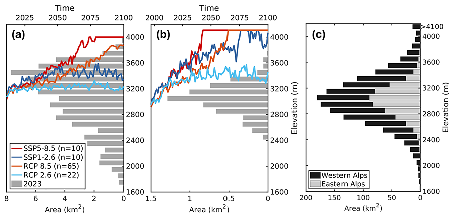
Figure 15 Area-elevation distribution of GAG (a), HEF (b) and all glaciers in the western and eastern Alps. Distribution of glacier area per 100 and 50 m elevation bands for and GAG (a) and HEF (b), respectively, for the year 2023 (with respect to bottom x-axis). Coloured lines show the evolution of the ELA of the four scenarios SSP5-8.5, SSP1-2.6, RCP 8.5 and RCP 2.6. (with respect to top x-axis). Distribution of glacier area per 100 and 50 m elevation bands for all glaciers in the western and eastern Alps based on RGI6.0 (Farinotti et al., 2009).

The generalization of our modelling results to a larger area is based on a specific model combination approach applied to two individual glaciers. Further modelling attempts based on standardized tests are necessary to infer how our modelling approach can be used to improve regional-scale glacier projections. In addition, follow-up studies focussing on glaciers with a sufficient data basis for our approach facilitate the generalization or extrapolation to a larger area.

8 Conclusions

We applied a three-dimensional full-Stokes ice-flow model to project the evolution of the Great Aletsch Glacier and Hintereisferner, considered as representative valley glaciers for the European Alps. Our modelling framework diverges significantly from large-scale modelling efforts, yet remains consistent with their overall findings. Under all climate scenarios, both glaciers are projected to lose a substantial volume of ice or complete deglaciation until the end of this century. Particularly, the retreat of Hintereisferner appears unavoidable even under sustained climate scenarios (inline with the political target negotiated in the Paris Agreement) compared to high-emission scenarios. The predicted 21st century retreat of the Great Aletsch Glacier is dramatic, although under sustained climate scenarios a portion of the Great Aletsch Glacier is likely to persist by 2100, but the decline in glacier volume seems to continue after the projection end date of 2100. Our findings indicate that glaciers in the eastern European Alps are likely to diminish by the mid-21st century, and only larger glaciers with higher area-elevation distribution will likely remain until the end of the century. The near-total disappearance of glaciers in the European Alps is expected to affect water availability, pose hazards in a deglaciating environment, and impact tourism and the economy.

A comparison of our glacier volume projections with previous studies reveals a large spread. The sources of projection differences are difficult to disentangle as there are several factors influencing the projections. It remains difficult to determine whether a more physically-based methodology (e.g., full-Stokes versus simpler models, surface energy balance models versus temperature index models) is essential for narrowing uncertainties in projections, as factors such as the initialization approach, the calibration strategy of uncertain parameters, and the handling of climate data might exert a comparable or even larger influence on the projections. Consequently, the development of standardized tests for model intercomparison between individual glacier modelling to large-scale modelling would be of considerable value to foster model improvements. Such a comparison is beyond the primary focus of the Glacier Model Intercomparison Project GlacierMIP (GlacierMIP 2025), a framework for a coordinated intercomparison of global-scale glacier models and related studies (Hock et al., 2019; Marzeion et al., 2020; Zekollari et al., 2019; Schuster et al., 2023), but would even complement and enhance this effort.

Appendix A

A1 Calculation of specific humidity

For running the EBM the variable near-surface specific humidity needs to be known. However, this variable is not provided by the ERA5 climate dataset that is used as forcing, and needs to be calculated instead. On the basis of dew point temperature (T_d, in °C) and surface pressure (p, in mb) specific humidity (q, in kg kg⁻¹) can be calculated as:

$$\begin{array}{}\text{(A1)}& q=\mathrm{0.622}{\displaystyle \frac{P}{p-\mathrm{0.378}P}}.\end{array}$$

Here, the vapour pressure (P in mb) can be calculated following the Magnus equation (Alduchov and Eskridge, 1996):

$$\begin{array}{}\text{(A2)}& P=\mathrm{6.112}\exp \left({\displaystyle \frac{\mathrm{17.62}{T}_{\mathrm{d}}}{T_{\mathrm{d}}+\mathrm{243.12}}}\right).\end{array}$$

A2 L-curve plots

The L-curve represents the tradeoff between two quantities that both need to be controlled: the data misfit between model and observations (the first term in Eq. 10, J₀) and the regularization term (the last term in Eq. 10, J_reg). The L-curve analysis involves computing J₀ and J_reg for a range of values of λ in Eq. (12). The resulting L-curves for each glacier are shown in Fig. A1.

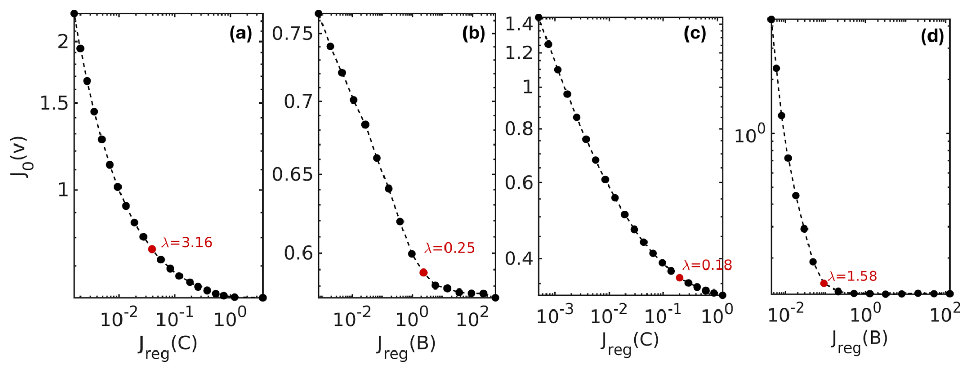
Figure A1 L-curves of the inversion for the basal friction coefficient (a, c) and the rheology B parameter (b, d) for HEF (a, c) and GAG (b, d). The selected regularization parameter λ of each inversion is highlighted in red.

A3 DInSAR surface velocity of Hintereisferner

Differential Synthetic Aperture Radar Interferometry (DInSAR) is a highly effective technique for measuring glacier movements by analyzing phase differences between SAR images acquired at different times. Using a known digital elevation model (DEM) to account for topographic effects, DInSAR can isolate motion-related phase changes, allowing accurate measurement of glacier surface velocity and flow patterns. This approach has been widely applied in glaciology, for instance, to monitor glacier dynamics in Greenland and Antarctica, offering insight into spatial and temporal variations in flow velocity (Rignot et al., 2011). The use of a DEM simplifies the processing chain and improves the reliability of deformation measurements (Nela et al., 2019), making DInSAR a valuable tool for studying glacier responses to climate change (Joughin et al., 2010).

The potential of this technique to map the motion field of small alpine ice and rock glaciers was initially explored two decades ago (Nagler et al., 2002; Gutjahr et al., 2004), utilizing ERS-1/2 data and focussing on the Hintereisferner test site, as also addressed in the current study. Hence, it is evident that both the data and the general workflow were established during that period. However, significant advancements have occurred over the past twenty years in both understanding of data and the methodologies employed for data processing. Regarding data understanding, notable progress includes the consistent reprocessing of ERS-1/2 orbits (Otten and Visser, 2019) and upgrading the DEM of the SRTM-C band DEM to version 4.1 (Jarvis et al., 2008). In terms of processing methodologies, advances such as the development of phase filters (Li et al., 2008) and phase unwrapping techniques, exemplified by the latest release of the Statistical-cost, Network-flow Algorithm for Phase Unwrapping (SNAPHU) by Chen and Zebker (2002) in February 2024, have significantly enhanced capabilities.

Table A1 summarizes the ERS-1/2 interferograms utilized in this study to derive the motion field of the Hintereisferner test site using the two-pass differential SAR interferometry approach (Kenyi and Kaufmann, 2003). To enhance coregistration and optimize the imaging geometry, all other available ERS-1/2 SLCs from the year 1996 were incorporated into the preparatory steps.

Table A1 ERS-1/2 Interferograms used in this study.

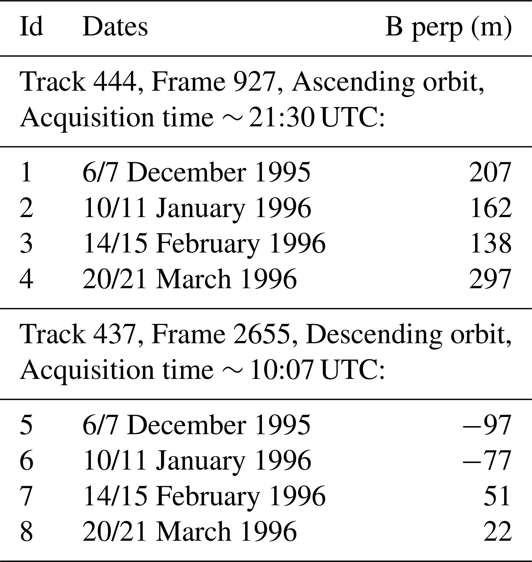
The ascending and descending stacks were processed independently up to the conversion of differential interferograms into line-of-sight (LOS) displacements. Finally, the equations described by Yin and Busch (2018) were applied to transform the orbit-dependent LOS displacements into the east-west and up-down components of the underlying three-dimensional deformation pattern. All differential interferograms calculated are shown in Fig. A2.

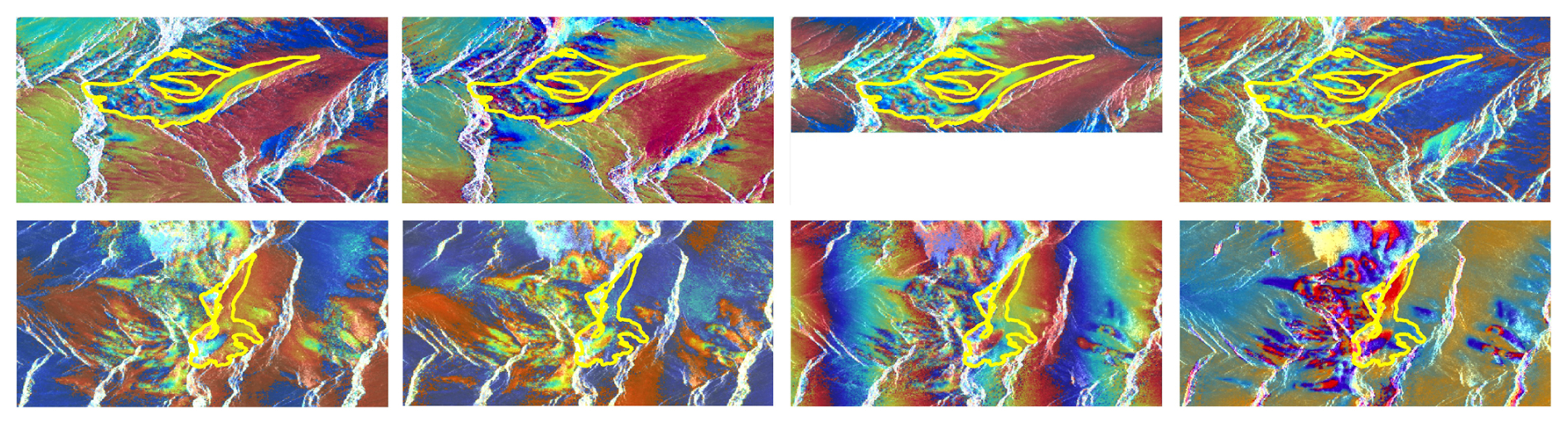
Figure A2 Colorized differential interferograms. Yellow line shows the 1998 glacier outline. Top row: Ascending orbit. Bottom row: Descending orbit. From left to right: 6/7 December 1995, 10/11 January 1996, 14/15 February 1996 and 20/21 March 1996.

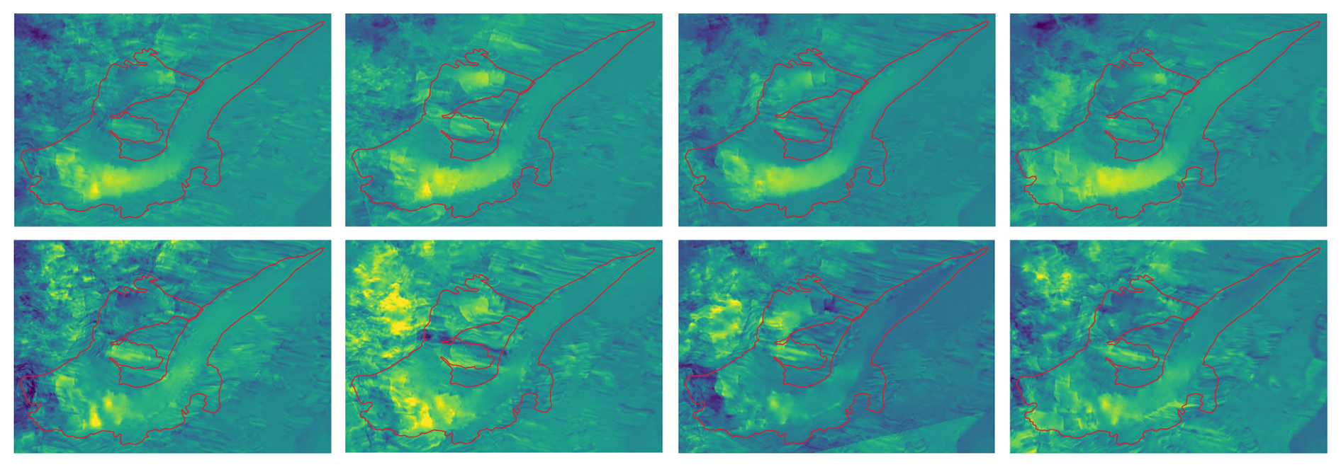
Figure A3 Interferometric glacier motion. Red line shows the 1998 glacier outline. Top row: East-west component [stretch −10 to 10 cm d⁻¹]. Bottom row: Up-down component [stretch −3 to 3 cm d⁻¹]. From left to right: 6/7 December 1995, 10/11 January 1996, 14/15 February 1996 and 20/21 March 1996.