Simulating liquid water distribution at the pore scale in snow: water retention curves and effective transport properties

Liquid water flows by gravity and capillarity in snow, drastically modifying its properties. Unlike dry snow, observing wet snow remains a challenge and data from 3D pore-scale imaging are scarce. This limitation hampers our understanding of the water, heat, and vapor transport processes in wet snow, as well as their modeling. Here, we explore a simulation-based approach, namely a pore morphology model, to simulate the distribution of liquid water in the pore space of snow for various water contents. Using the Young-Laplace equation and pore radius as a probe, liquid water is gradually introduced and then removed during wetting (imbibition) and drying (drainage) simulations, respectively. This model was applied to a set of 34 3D tomography images of dry snow of varied microstructures. For each microstructure, a series of 3D images of wet snow at different stages of drainage and imbibition was obtained. From these series, we examine key properties for the modeling of wet snow processes. First, we describe the water retention curves obtained for imbibition and drainage for the different microstructures. The classical van Genuchten model is used to describe our simulated water retention curves. The obtained model parameters, i.e., the shape parameters (α_vg and n_vg) and the residual water content, are compared to the ones obtained in laboratory experiments from literature. New parameterizations of these parameters based on snow density, grain size, and the interfacial mean curvature are proposed. Then, we present estimates of hydraulic conductivity, water permeability, effective thermal conductivity, and water vapor diffusivity, computed on the simulated wet snow images. We study their evolution in relation to water content, density, and snow type. Our estimates are compared to existing parameterizations of the wet snow properties; new parameterizations are proposed when needed. Our simulations are a first step toward a better characterization of the micro-scale distribution of liquid water in snow, and contribute to improving the modeling of the hydraulic and physical properties of wet snow.

1 Introduction

Wet snow is characterized by the presence of liquid water in the dry snow microstructure itself, composed of air and ice. Liquid water, introduced by rain or melt, is transported in the snowpack and causes drastic changes in the microstructures and properties of the snow, which can lead to wet snow avalanches (e.g., Schweizer et al., 2003) or the release of large amounts of water and flooding (e.g., Singh et al., 1997). The rapid morphological transformation of the wet snow microstructure is called wet snow metamorphism (e.g., Wakahama, 1968; Colbeck, 1973; Raymond and Tusima, 1979; Marsh and Woo, 1985) and is characterized by the formation of large, rounded, often clustered grains, referred to as melt forms (Fierz et al., 2009). Liquid water transport in snow is a complex phenomenon that involves water flow by gravity and capillarity (e.g. Gerdel, 1954; Colbeck, 1976). It can present features such as preferential flow (e.g. Hirashima et al., 2014), capillary rise (e.g. Lombardo et al., 2025), capillary barriers (e.g. Quéno et al., 2020), or hysteretic wetting-drying processes (e.g. Adachi et al., 2020). Liquid water transport is coupled with heat and water vapor transport, driven by heat conduction (e.g. Sturm et al., 1997), heat convection (e.g. Sturm and Johnson, 1991), latent heat and vapor fluxes from phase changes (e.g. Calonne et al., 2014b), and vapor diffusion (e.g. Fourteau et al., 2021). Several models have been proposed to simulate wet snow and water transport in the snowpack, (e.g., Daanen and Nieber, 2009; Hirashima et al., 2014; Wever et al., 2016; Leroux and Pomeroy, 2017; Moure et al., 2023; Jones et al., 2024), including large-scale operational models such as Crocus (Vionnet et al., 2012; Fourteau et al., 2025; Lafaysse et al., 2025) and Snowpack (Lehning et al., 2002; Wever et al., 2014, 2015).

The movement of water is classically described by the Richards equation, which expresses the volumetric liquid water content evolution in unsaturated porous media (Richards, 1931):

$$\begin{array}{}\text{(1)}& {\displaystyle \frac{\partial {\mathit{\theta }}_{\mathrm{w}}}{\partial t}}={\displaystyle \frac{\partial }{\partial z}}\left({\mathbb{K}}_{\mathrm{w}}^{\mathrm{u}}\left({\mathit{\theta }}_{\mathrm{w}}\right)\left({\displaystyle \frac{\partial h}{\partial z}}+\mathrm{1}\right)\right)-S\end{array}$$

with θ_w (–) the volumetric water content, h (m) the liquid pressure head (linearly related to the capillary pressure), ${\mathbb{K}}_{\mathrm{w}}^{\mathrm{u}}$ (m s⁻¹) the unsaturated hydraulic conductivity, S (s⁻¹) a source/sink term, and z the vertical direction pointing upwards. To solve this equation, the liquid pressure head and the unsaturated hydraulic conductivity need to be specified. In general porous media applications, the water content θ_w is expressed as a function of the liquid pressure head h through the water retention curve (WRC). The WRC describes the evolution of capillary pressure in pores as a function of water content, which reflects the hydraulic behavior of the porous medium. This relationship can be obtained for primary imbibition, which corresponds to the wetting of a dry porous medium by a liquid until it reaches saturation, for primary drainage, which corresponds to the drainage of a fully saturated porous medium, and for drainage or imbibition of a porous medium at any intermediate state of saturation.

WRCs are traditionally derived based on laboratory experiments, in which the liquid pressure head in the porous material under study is measured during a drainage or imbibition experiment, at different water contents. For snow, some WRC measurements are available (e.g., Colbeck, 1974; Coléou et al., 1999; Yamaguchi et al., 2010, 2012; Katsushima et al., 2013; Adachi et al., 2020; Lombardo et al., 2025). They, however, show different limitations. In these studies, the liquid pressure head was typically measured with a coarse vertical resolution on the order of centimeters, except for Adachi et al. (2020), who provide measurements at a spatial resolution of 2 mm based on the magnetic resonance imaging method (MRI), and Lombardo et al. (2025), who provide measurements at 92 µm using neutron radiography. Another limitation concerns the snow samples under study, which, in the majority, were dense melt forms. The measurements of Yamaguchi et al. (2012) are the most extensive, based on 60 snow samples, yet restricted to sieved or natural melt forms and natural rounded grains, with high density values from 360 to 630 kg m⁻³, and grain sizes from 0.3 to 5.8 mm. These results highlight the need to extend our knowledge on the impact of snow microstructure on the WRCs to a broader range of snow types. Finally, most of the WRC measurements were performed for drainage; only Coléou et al. (1999), Adachi et al. (2020), and Lombardo et al. (2025) provided experimental WRCs for imbibition.

Besides direct measurements, WRCs can be described using the widely-used van Genuchten (VG) model, initially developed for soils (van Genuchten, 1980). The VG model reads:

$$\begin{array}{}\text{(2)}& {\displaystyle }{S}_{\mathrm{e}}\left(h\right)={\displaystyle \frac{{\mathit{\theta }}_{\mathrm{w}}\left(h\right)-{\mathit{\theta }}_{\mathrm{w}}^{\mathrm{r}}}{{\mathit{\theta }}_{\mathrm{w}}^{\mathrm{s}}-{\mathit{\theta }}_{\mathrm{w}}^{\mathrm{r}}}}={\left(\mathrm{1}+({\mathit{\alpha }}_{\text{vg}}h{)}^{n_{\text{vg}}}\right)}^{-m_{\text{vg}}}\end{array}$$

The term S_e(h) corresponds to the effective water saturation (e.g., Mualem, 1976; d'Amboise et al., 2017). ${\mathit{\theta }}_{\mathrm{w}}^{\mathrm{r}}$ and ${\mathit{\theta }}_{\mathrm{w}}^{\mathrm{s}}$ are the residual water content after drainage and the maximum water content reached during imbibition, respectively. α_vg, n_vg, and m_vg are the adjusted parameters of the VG model that determine the shape of the WRC. These shape parameters depend on the material's morphology and need to be specified. For that, regressions to estimate the shape parameters from microstructural properties were developed by fitting the VG model to WRCs obtained experimentally. For snow, Daanen and Nieber (2009) and Yamaguchi et al. (2010) proposed regressions based on snow grain size, developed from a few drainage experiments on similar snow samples composed of dense melt forms. Later, Yamaguchi et al. (2012) presented improved regressions based on both snow density and grain size, using additional drainage experiments, but based on the WRCs of the snow samples made of sieved melt forms only, thus limiting the validation of the regressions to coarse-grained, high-density snow. To date, no regression of the shape parameters of the VG model has been presented specifically for imbibition in snow.

The water unsaturated hydraulic conductivity ${\mathbb{K}}_{\mathrm{w}}^{\mathrm{u}}$, which is the second unknown of the Richards equation (Eq. 1), can be expressed as a function of the liquid water content θ_w as:

$$\begin{array}{}\text{(3)}& {\mathbb{K}}_{\mathrm{w}}^{\mathrm{u}}\left({\mathit{\theta }}_{\mathrm{w}}\right)={\mathbb{K}}_{\mathrm{w}}^{\text{sat}}\times K_{\mathrm{w}}^{\mathrm{r}}\left({\mathit{\theta }}_{\mathrm{w}}\right)\end{array}$$

where ${\mathbb{K}}_{\mathrm{w}}^{\text{sat}}=K{\mathit{\rho }}_{\mathrm{w}}g/{\mathit{\mu }}_{\mathrm{w}}$ is the saturated hydraulic conductivity of snow (m s⁻¹), which depends on the intrinsic permeability of snow K (m²), on the water viscosity μ_w (Pa s), on the water density ρ_w (kg m⁻³), and on the gravitational acceleration g (m s⁻²). The intrinsic permeability of snow K depends solely on the microstructure of dry snow and can be estimated from empirical parameterizations, such as the one of Shimizu (1970) based on measurements or the one of Calonne et al. (2012) based on numerical computations on 3D tomographic images of snow. The term $K_{\mathrm{w}}^{\mathrm{r}}\left({\mathit{\theta }}_{\mathrm{w}}\right)$ corresponds to the relative water permeability at a given saturation, and is defined as $K_{\mathrm{w}}^{\mathrm{r}}\left({\mathit{\theta }}_{\mathrm{w}}\right)=K_{\mathrm{w}}^{\mathrm{u}}\left({\mathit{\theta }}_{\mathrm{w}}\right)/K$, $K_{\mathrm{w}}^{\mathrm{u}}\left({\mathit{\theta }}_{\mathrm{w}}\right)$ being the unsaturated water permeability. The unsaturated water permeability $K_{\mathrm{w}}^{\mathrm{u}}\left({\mathit{\theta }}_{\mathrm{w}}\right)$, or equivalently the relative water permeability $K_{\mathrm{w}}^{\mathrm{r}}\left({\mathit{\theta }}_{\mathrm{w}}\right)$, are classically modeled using the van Genuchten–Mualem (VGM) equation for unsaturated soils, which relates the permeability $K_{\mathrm{w}}^{\mathrm{u}}$ to the liquid water content θ_w (Mualem, 1976; van Genuchten, 1980). The VGM equation is written as:

$$\begin{array}{}\text{(4)}& K_{\mathrm{w}}^{\mathrm{u}}\left(S_{\mathrm{e}}\right)=K\times S_{\mathrm{e}}^{{\mathit{\tau }}_{\text{vg}}}{\left(\mathrm{1}-(\mathrm{1}-S_{\mathrm{e}}^{\mathrm{1}/m_{\text{vg}}}{)}^{m_{\text{vg}}}\right)}^{\mathrm{2}}\end{array}$$

where the shape parameters α_vg, n_vg, and m_vg are the same as those defined in the VG model (Eq. 2). The exponent τ_vg describes the effects of the connectivity and tortuosity of the flow paths (e.g., Mualem, 1976; Vereecken et al., 2010). The estimation of the unsaturated hydraulic conductivity of snow is affected by the same limitations as those described for the estimation of the WRCs of snow.

The processes of heat transport and water vapor transport in wet snow are driven by the unsaturated effective thermal conductivity of snow k^u(θ_w) and the unsaturated effective water vapor diffusivity of snow D^u(θ_w), which have been little studied. These properties were investigated for dry snow, in particular using X-ray tomography, which provides the 3D distribution of the ice and air structure at the pore scale, thus enabling accurate computations (e.g., Kaempfer et al., 2005; Calonne et al., 2011, 2014b; Fourteau et al., 2021; Bouvet et al., 2022). The modeling of heat and vapor transport in dry snow could thus be improved in macro-scale models (e.g., Calonne et al., 2014b; Hansen and Foslien, 2015; Calonne et al., 2015; Brondex et al., 2023; Bouvet et al., 2024). These advances are, however, limited to dry snow. Performing X-ray tomography on wet snow samples is still a challenge, notably due to the lack of contrast between the X-ray absorption of ice and liquid water. The literature studies generally propose refrozen states of wet snow (e.g., Flin et al., 2011; Avanzi et al., 2017) which do not allow a precise imaging of the ice-water interface. Direct 3D imaging of wet snow is presently only achieved by MRI (Adachi et al., 2020; Yamaguchi et al., 2025), with mm-scale images, whereas observing pore-scale processes requires a µm-scale resolution. Due to these limitations, wet snow models rely on simple approaches to estimate the effective properties of wet snow. In many models (Daanen and Nieber, 2009; Leroux and Pomeroy, 2017; Moure et al., 2023), the unsaturated thermal conductivity of snow k^u is derived based on an arithmetic mean, such as k^u = $k_{\text{dry}}^{\text{eff}}(\mathrm{1}-{\mathit{\theta }}_{\mathrm{w}})+k_{\mathrm{w}}{\mathit{\theta }}_{\mathrm{w}}$, with $k_{\text{dry}}^{\text{eff}}$ the effective thermal conductivity of dry snow and k_w the intrinsic thermal conductivity of liquid water. In doing so, the impact of the microstructure and phase connectivity is not fully considered, although their importance was shown in dry snow (Calonne et al., 2011). In the operational Crocus model (Vionnet et al., 2012; Lafaysse et al., 2025), the parameterization of Yen (1981), which is only valid for dry snow, is extrapolated to wet snow, leading to the assumption that ice and water have the same impact on the snow effective thermal conductivity, although ice conducts four times more than water. Finally, the unsaturated effective water vapor diffusivity of snow has not yet been studied, as water vapor transport by diffusion has not yet been implemented in wet snow models. For unsaturated soils, different parameterizations are used depending on the soil nature, such as the ones of Millington and Quirk (1961) and Moldrup et al. (2000) (see Kristensen et al., 2010).

Different methods are currently used to compute the WRCs within porous media from 3D images of their microstructure. The first approach consists in performing two-phase flow simulations at the pore scale using different numerical methods, such as the lattice-Boltzmann method (Vogel et al., 2005; Ahrenholz et al., 2008), the volume of fluids method (Bhatta et al., 2024), or the phase-field modeling (Prodanović and Bryant, 2006; Jettestuen et al., 2013). These simulations accurately describe the dynamics of the physical processes at the pore-scale, but they require substantial computational resources when applied to complex 3D microstructures. To overcome this drawback, other methods such as the Pore Network Model (PNM) (Vogel et al., 2005; Joekar-Niasar and Hassanizadeh, 2012; Xiong et al., 2016) or the Pore Morphology Method (PMM) (Hilpert and Miller, 2001; Silin and Patzek, 2006; Ahrenholz et al., 2008; Berg et al., 2016; Liu et al., 2022; Arnold et al., 2023; Suh et al., 2024) can be used. The PNM consists of creating a virtual representation of the porous medium, consisting of pore bodies (nodes) and pore throats (edges) of different sizes connected to each other. It is then possible to simulate the fluid flow and other transport processes of interest at the meso-scale through this network, with the relevant 1D physics implemented between nodes. The construction of such a model requires the extraction of microstructural parameters from the 3D images, such as pore sizes, throat sizes, coordination number, or shape factor, which is not always straightforward and impacts the accuracy of the modeling (see Xiong et al., 2016, and references herein). In the quasi-static regime, the Pore Morphology Method (PMM) can be used to compute, from a 3D image, the fluid phase distribution through a series of image-processing operations without solving any partial differential equation. The obtained 3D images, corresponding to different water content values in the porous medium, can then be used to compute the effective properties such as permeability, thermal conductivity, or effective diffusivity (Berg et al., 2016; Becker et al., 2008).

In the present paper, the Pore Morphology Method (PMM) is used to compute the WRCs during imbibition and drainage of snow. The ice structure is fixed, i.e., the wet snow metamorphism is not represented. The PMM is applied to 34 experimental 3D tomography images of dry snow, presenting a wide range of snow microstructures, in terms of density, grain size, and shape. A series of 3D images is obtained, showing distributions of air, ice, and liquid water in snow at different stages of drainage or imbibition, so for different liquid water contents. The first part of this work is dedicated to the study of the WRCs, which are directly obtained from the simulations. The impact of the snow microstructure on the WRC shape is analyzed. The simulated WRCs are compared to experimental WRCs from the literature, including a comparison of the adjusted parameters of the VG model. New regressions of these parameters are proposed for both imbibition and drainage and compared to existing ones. In the second part, the series of 3D snow images at different stages of drainage or imbibition are used to compute the effective properties required for the modeling of water flow, heat, and vapor transport in wet snow. The studied properties are the relative permeability (i.e. the unsaturated hydraulic conductivity), the effective thermal conductivity, and the effective water vapor diffusivity. The numerical results are compared with commonly used estimates from the literature, such as the VGM model for the unsaturated hydraulic conductivity. New regressions of effective thermal conductivity and vapor diffusivity are presented to account for the level of water saturation.

2 Methods

2.1 Definition of the micro-scale variables

Within the representative elementary volume (REV) of snow noted Ω, we define Ω_i, Ω_w, and Ω_a the volumes occupied by the ice, the water, and the air phase, respectively, as illustrated in Fig. 1. The volume fractions θ of the different phases (ice, water, air) are written:

$$\begin{array}{}\text{(5)}& {\mathit{\theta }}_{\mathrm{i}}={\displaystyle \frac{{\mathrm{\Omega }}_{\mathrm{i}}}{\mathrm{\Omega }}},{\mathit{\theta }}_{\mathrm{w}}={\displaystyle \frac{{\mathrm{\Omega }}_{\mathrm{w}}}{\mathrm{\Omega }}},{\mathit{\theta }}_{\mathrm{a}}={\displaystyle \frac{{\mathrm{\Omega }}_{\mathrm{a}}}{\mathrm{\Omega }}},\end{array}$$

with ${\mathit{\theta }}_{\mathrm{i}}+{\mathit{\theta }}_{\mathrm{w}}+{\mathit{\theta }}_{\mathrm{a}}=\mathrm{1}$. The porosity ϕ, the water saturation S_w and air saturation S_a are, respectively defined as:

$$\begin{array}{}\text{(6)}& \mathit{\varphi }={\displaystyle \frac{\mathrm{1}-{\mathrm{\Omega }}_{\mathrm{i}}}{\mathrm{\Omega }}}={\displaystyle \frac{{\mathrm{\Omega }}_{\mathrm{a}}+{\mathrm{\Omega }}_{\mathrm{w}}}{\mathrm{\Omega }}},S_{\mathrm{w}}={\displaystyle \frac{{\mathrm{\Omega }}_{\mathrm{w}}}{{\mathrm{\Omega }}_{\mathrm{a}}+{\mathrm{\Omega }}_{\mathrm{w}}}},S_{\mathrm{a}}={\displaystyle \frac{{\mathrm{\Omega }}_{\mathrm{a}}}{{\mathrm{\Omega }}_{\mathrm{a}}+{\mathrm{\Omega }}_{\mathrm{w}}}},\end{array}$$

which leads to:

$$\begin{array}{}\text{(7)}& \begin{array}{rl}& \mathit{\varphi }=\mathrm{1}-{\mathit{\theta }}_{\mathrm{i}},S_{\mathrm{w}}+S_{\mathrm{a}}=\mathrm{1},{\mathit{\theta }}_{\mathrm{w}}=\mathit{\varphi }{S}_{\mathrm{w}},\text{and}\\ & {\mathit{\theta }}_{\mathrm{a}}=\mathit{\varphi }{S}_{\mathrm{a}}=\mathit{\varphi }(\mathrm{1}-S_{\mathrm{w}}).\end{array}\end{array}$$

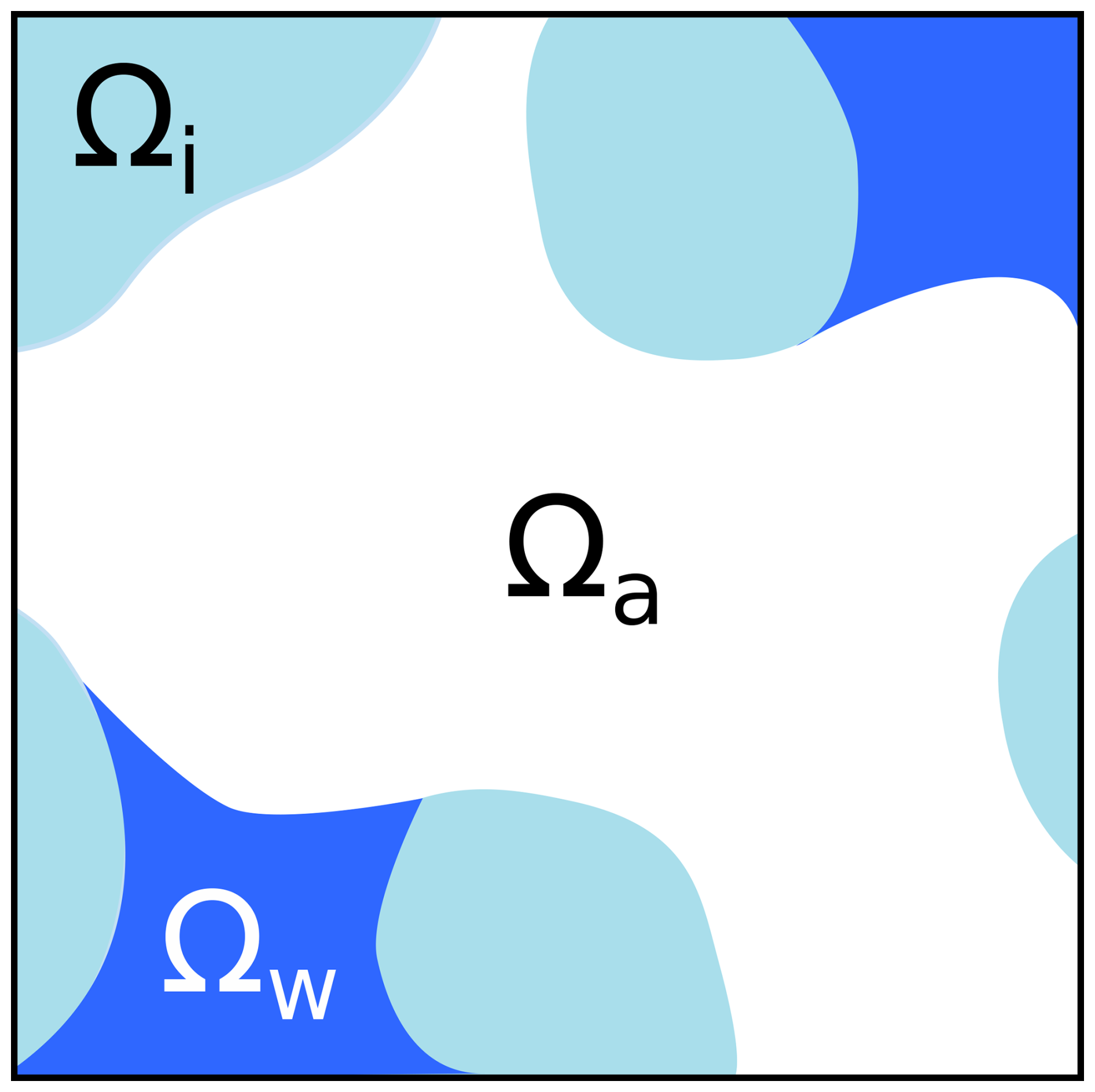
Figure 1 Illustration of the micro-scale air (white), ice (light blue), and liquid water (dark blue) phases in wet snow. Ω_a, Ω_i, and Ω_w represent the volume of air, ice, and liquid water, respectively.

2.2 3D images of snow and microstructural properties

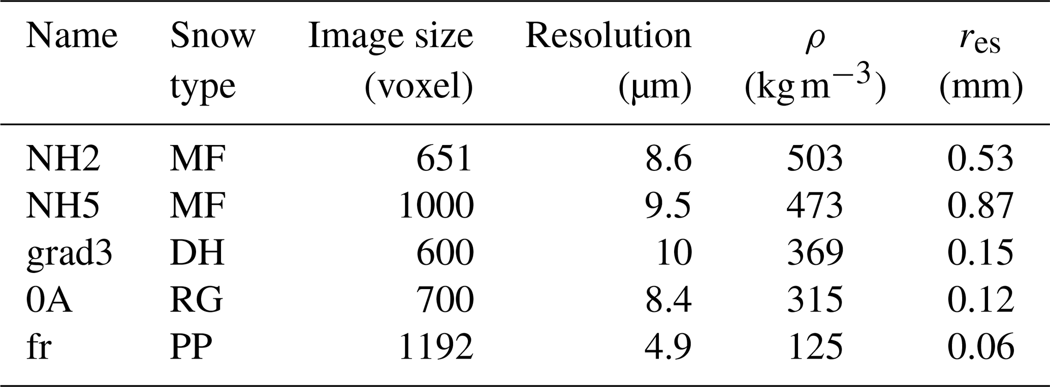
The set of 3D images of snow used in this study for the simulations corresponds to the one from Calonne et al. (2012) (see the related Supplement for details). This set consists of 34 images of different dry snow microstructures obtained by X-ray micro-tomography, covering a wide range of snow properties in terms of density, grain size, and snow type. The imaged snow samples are composed of natural snow collected in the field as well as snow obtained from evolution under controlled environmental conditions in cold laboratory, which replicates natural snow evolution. The image volumes are cubic, with sides ranging in size from ∼ 2.5 to 10 mm and resolution from ∼ 5 to 10 µm. Of these 34 images, 5 images representative of the diversity of all the images were selected for detailed investigations. They include two images of melt forms at different densities and grain sizes, and one image of depth hoar, rounded grains, and precipitation particles. Their main characteristics are shown in Table 1. To characterize these dry snow microstructures, we rely on the snow density ρ in kg m⁻³ (in the following the snow density will always refer to the dry density without liquid water), which is computed from the snow porosity as $\mathit{\rho }=(\mathrm{1}-\mathit{\varphi })/{\mathit{\rho }}_{\mathrm{i}}$, with ρ_i the ice density taken as 917 kg m⁻³, and the spherical equivalent radius r_es in m, derived from the specific surface area (SSA, m² kg⁻¹) as $r_{\text{es}}=\mathrm{3}/(\text{SSA}\times {\mathit{\rho }}_{\mathrm{i}})$ with ρ_i the ice density. Snow density and SSA values were provided by Calonne et al. (2012) (see the related Supplement for the detailed table) based on 3D image computations using simple voxel counting and a stereological method (Flin et al., 2011).

Table 1 Main characteristics of the 5 selected 3D images. The image size is the side length of the cubic image. Snow types are given according to the international classification (Fierz et al., 2009).

2.3 Numerical simulations of imbibition and drainage

The SatuDict module of the Geodict software (Math2Market GmbH) (Thoemen et al., 2008) based on the Pore Morphology Method (PMM) (e.g., Hilpert and Miller, 2001; Silin and Patzek, 2006; Schulz et al., 2015; Berg et al., 2016; Liu et al., 2022; Arnold et al., 2023) was used to compute water retention curves (WRCs) of snow. This method, valid in a quasi-static regime, is applicable when the gravity and viscous forces are negligible compared to capillary forces, which is the case in snow. Indeed, at the pore scale, capillary forces usually play a much more important role than gravity. For air and water, the Bond number, which measures the ratio between gravitational force and surface tension force, is defined as: $\text{Bo}=({\mathit{\rho }}_{\mathrm{w}}-{\mathit{\rho }}_{\mathrm{a}})g{l}^{\mathrm{2}}/\mathit{\gamma }$ where ρ_w and ρ_a are the water and the air density, respectively, g is the gravity, γ the surface tension, and l is a characteristic length of the snow microstructure at the pore scale, such as the pore size. This dimensionless number varies between 10⁻³ and 10⁻¹ for a pore size l varying between 10⁻⁴ and 10⁻³ m as in snow. These estimations show that gravitational forces are negligible at the pore scale in comparison to capillary forces. Similarly, it can be shown (Auriault, 1987; Auriault et al., 2009) that within a porous medium for small Reynolds numbers and capillary numbers, the viscous stress (σ_v) at the pore scale is negligible in comparison to the fluid pressure (p). The latter is of the order of the capillary pressure (p_c): $p\approx p_{\mathrm{c}}\approx (L/l){\mathit{\sigma }}_{\mathrm{v}}$ where L is a macroscopic length, i.e. the characteristic size of the snowpack. If we assume that l = 10⁻³ m and L = 0.1 m, the capillary pressure is around 100 times larger than the viscous stress.

The PMM uses a sphere with a radius r as a probe to detect the pore space that is accessible by the non-wetting phase (NWP, here the air). This radius is computed from the Young–Laplace equation: $r=\mathrm{2}\mathit{\gamma }\text{cos}\left(\mathit{\psi }\right)/p_{\mathrm{c}}$ where p_c is the capillary pressure, γ is the surface tension, and ψ is the contact angle between ice and liquid water. At 0 °C, γ = 0.0756 N m⁻¹ and ψ = 12° (Knight, 1967). Morphological operations, namely, erosion and/or dilation, are used in the PMM (Hilpert and Miller, 2001). The algorithm of the PMM can be decomposed into several steps as follows (see e.g. Fig. 2 in Arnold et al., 2023):

• In drainage conditions, the porous medium is initially saturated with the wetting phase (WP, here the water) and p_c = 0. The invading NWP is connected to the inlet, which is the NWP reservoir, and the WP can escape through the outlet, the WP reservoir. (i) Then, p_c is increased incrementally, i.e. r is decreased incrementally. The solid phase is first dilated by a sphere with radius r. (ii) All the pores connected to the NWP reservoir are labeled as NWP. (iii) The NWP is then dilated with the same sphere with radius r. The remaining pores are filled with the WP. The saturation can then be calculated. (iv) All the pores filled by the WP disconnected from the WP reservoir are considered as WP residual, and are no longer considered in the next steps. All these steps (i to iv) are repeated by increasing the value of the pressure, i.e. by decreasing the value of r. In the present case, the radius r was decreased gradually with a step of 2 pixel size.

• In imbibition conditions, the porous medium is initially saturated with the NWP. The invading WP is connected to the inlet, which is the WP reservoir, and the NWP can escape the NWP reservoir through the outlet. (i) Then, p_c is decreased incrementally, i.e. r is increased incrementally. The solid phase is first dilated by a sphere with radius r. (ii) The NWP is then dilated with the same sphere with radius r. (iii) All the pores connected to the WP are now labeled as WP. The remaining pores are NWP. The saturation can then be calculated. (iv) All the pores filled by the NWP disconnected from the NWP reservoir are considered as NWP residual, and are no longer considered in the next steps. As for the drainage conditions, all these steps (i to iv) are repeated for the next value of the pressure, i.e. the next value of r. In the present case, the radius r was increased gradually with a step of 2 pixel size.

In imbibition conditions, if the step (iv) is ignored, the PMM also allows to compute the Mercury Injection Capillary Pressure (MICP) curves, which are a commonly-used technique for measurements of porosity or pore throat size distribution, for instance (Hilpert and Miller, 2001; Berg et al., 2016). As underlined in Hilpert and Miller (2001), the accuracy of the PMM may depend on the resolution and size of the 3D images and of the definition of the structural element. Finally, it is worth mentioning that the boundary conditions applied on the four sides of the 3D images that are not connected to the NWP or WP reservoirs may also play a role in the WRC simulations, even if this point has not been discussed in the literature, to the best of our knowledge. In Vogel et al. (2005), impervious boundary conditions are applied, whereas other conditions, such as symmetry, displaced fluid outlet, or invading fluid inlet, may also be applied (Berg et al., 2016). These boundary conditions may lead to different values of the NWP (air) residuals during the imbibition process, since these residuals can be trapped or not at the boundaries. Depending on the boundary conditions, the maximum water content (${\mathit{\theta }}_{\mathrm{w}}^{\mathrm{s}}$) may range from 45 % to 90 % of the porosity. Despite such large differences, the values of α_vg and n_vg in the Van Genuchten (VG) model (van Genuchten, 1980) remains almost constant (Likos et al., 2013; Farooq et al., 2024, see also Sect. 4). The impact of the boundary conditions is less pronounced in drainage conditions, since the water residuals are mainly located at the junction between closegrains.

In the present study, the PMM implemented in the SatudDict software was used to compute the WRCs of the 34 snow samples. We computed (i) a primary imbibition curve assuming that there is no air (NWP) residuals as in MICP experiments, thus ${\mathit{\theta }}_{\mathrm{w}}^{\mathrm{s}}=\mathit{\varphi }$ in Eq. (2), and then (ii) a primary drainage curve until reaching the water (WP) residuals (${\mathit{\theta }}_{\mathrm{w}}^{\mathrm{r}}$ in Eq. 2). In both cases, symmetric boundary conditions were applied on the four sides of the volumes. The series of 3D snow images at different stages of drainage were then used to compute the relative permeability (i.e. the unsaturated hydraulic conductivity), the effective thermal conductivity, and the effective water vapor diffusivity.

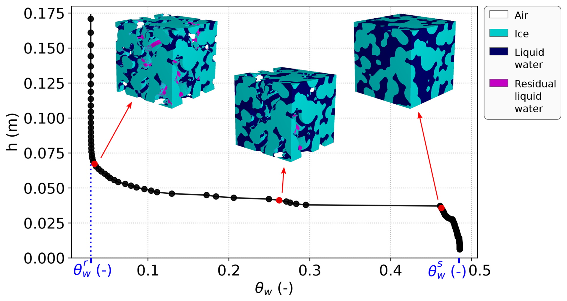
Figure 2 Example of a water retention curve estimated from a drainage simulation on the 3D tomographic snow sample NH5 (MF). The simulated 3D water distribution in the pores is shown at 3 different stages.

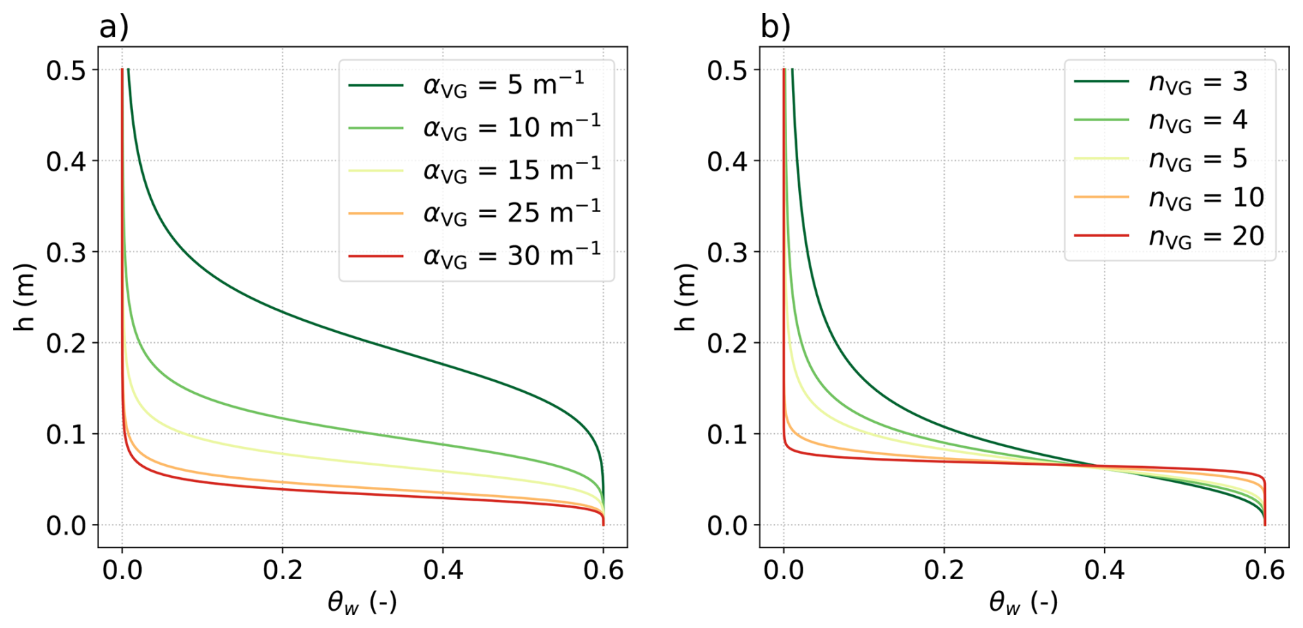
Figure 3 WRCs from the VG model: influence of (a) the parameter α_vg (with a fixed n_vg = 5) and of (b) the parameter n_vg (with a fixed α_vg = 15 m⁻¹).

2.4 Water retention curve analysis

Results from the SatuDict software are used to determine the WRC, by expressing the liquid pressure head h as a function of the liquid water volume fraction θ_w, for both imbibition and drainage. An example of the WRC obtained from a drainage simulation on a small MF sample is shown in Fig. 2. The plot should be read from right to left, as water is gradually drained out of the porous microstructure. The liquid pressure head increases with decreasing water content, characterized by a sharp rise at the very beginning and very end of drainage and a near constant value for the intermediate water contents. The 3D images show the distribution of the air (transparent) and water (dark blue) in the pore space of the snow at different points on the WRC. WRCs also provide the residual water content ${\mathit{\theta }}_{\mathrm{w}}^{\mathrm{r}}$, being the remaining water content after drainage, and the saturated water content ${\mathit{\theta }}_{\mathrm{w}}^{\mathrm{s}}$, being the maximum amount of water the snow volume can store. Here, ${\mathit{\theta }}_{\mathrm{w}}^{\mathrm{s}}=\mathit{\varphi }$ since no air residuals are simulated. Both parameters are illustrated in the figure as the endpoints of the WRC.

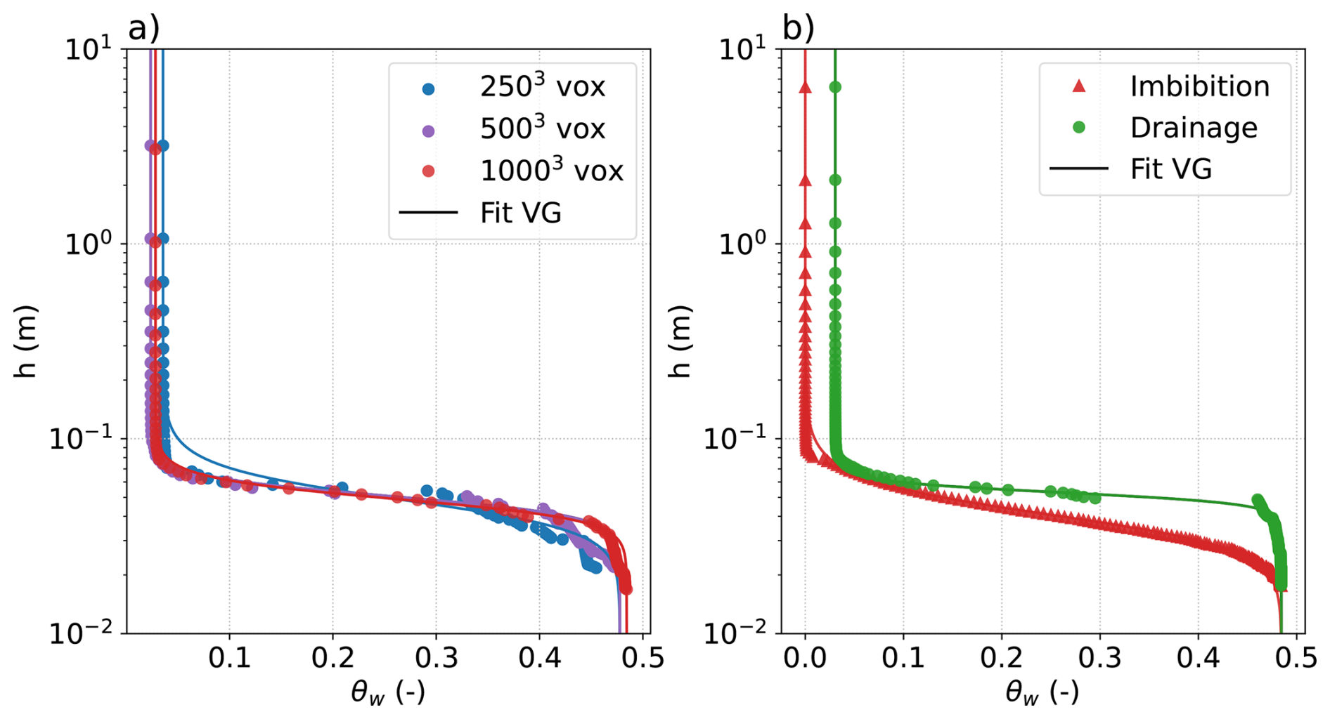
Figure 4 (a) Influence of the volume size taken for drainage simulations on the WRC, for the sample NH5 of melt forms. Simulation data are represented by symbols and the fitted VG models by solid lines. (b) Example of hysteresis of the WRC between imbibition and drainage, for the snow sample NH5.

To further analyze the WRCs estimated from the different snow images, the curves are fitted to the van Genuchten (VG) model (van Genuchten, 1980) described in the introduction and by Eq. (2). This model relies on the shape parameters α_vg, n_vg, and m_vg, which determine the shape of the WRC and need to be specified. The parameter m_vg is usually approximated by $m_{\text{vg}}=\mathrm{1}-\mathrm{1}/n_{\text{vg}}$ (e.g., Yamaguchi et al., 2010). The influence of the parameters α_vg and n_vg on the WRC is illustrated in Fig. 3. n_vg controls the steepness of the curve inflections while the inverse of α_vg is related to the values of h at which inflections occur. Roughly, the parameter α_vg can be related to the average pore size and n_vg to the width of the pore size distribution (e.g., Yamaguchi et al., 2010; van Lier and Pinheiro, 2018). In what follows, the WRCs of each imbibition and drainage simulation are considered and used to fit the VG model. For fitting, we took ${\mathit{\theta }}_{\mathrm{w}}^{\mathrm{s}}=\mathit{\varphi }$ for both imbibition and drainage, ${\mathit{\theta }}_{\mathrm{w}}^{\mathrm{r}}=\mathrm{0}$ for imbibition, and ${\mathit{\theta }}_{\mathrm{w}}^{\mathrm{r}}$ equals the minimum value of θ_w obtained from the drainage simulations for drainage. These choices are justified by the fact that our simulations start with a primary imbibition, without any liquid water in the pores, and that we do not simulate entrapped air in imbibition but residual water in drainage.

Finally, we evaluated the REV of the WRC on our 3D images, by performing imbibition and drainage simulations from several sub-volumes of increasing sizes within the same sample, as in Hilpert and Miller (2001). The size of the REV was assumed to be reached once values of the WRC did not vary significantly when the size of the sub-volumes of computation increased. Figure 4a shows an example for the sample NH5 (MF), which is the most critical sample because of its large grains. We see that the REV needed to obtain representative distributions of the fluids in the pores and representative WRCs is rather large compared to the typical REV of thermal conductivity, density, or SSA (e.g., Calonne et al., 2011; Flin et al., 2011). The maximum sizes available for all the 3D images were then used, giving satisfactory results.

2.5 Computation of the effective transport properties of wet snow

Next, we study the effective transport properties of wet snow based on the 3D image series obtained from the drainage simulations. We focus on the properties involved in the processes of heat, water vapor and liquid water transport, namely the water unsaturated hydraulic conductivity ${\mathbb{K}}_{\mathrm{w}}^{\mathrm{u}}$ (linked to the relative water permeability ${\mathbf{K}}_{\mathrm{w}}^{\mathrm{r}}\left({\mathit{\theta }}_{\mathrm{w}}\right)$), the unsaturated effective thermal conductivity of snow k^u(θ_w) and the unsaturated effective water vapor diffusivity of snow D^u(θ_w). To access ${\mathbf{K}}_{\mathrm{w}}^{\mathrm{u}}\left({\mathit{\theta }}_{\mathrm{w}}\right)$, k^u(θ_w) and D^u(θ_w), the Geodict software was used to compute the 3D tensors of these three transport properties of wet snow: the intrinsic water permeability ${\mathbf{K}}_{\mathrm{w}}^{\mathrm{u}}$ in m², the effective thermal conductivity k^u in $\mathrm{W}{\mathrm{m}}^{-\mathrm{1}}{\mathrm{K}}^{-\mathrm{1}}$ and the effective water vapor diffusivity D^u in m² s⁻¹. Computations were performed on the series of 3D images of wet snow obtained from the imbibition and drainage simulations, so for different water contents, snow densities, and microstructures. For each property, a specific boundary value problem, resulting from a homogenization technique, is solved on the REV, applying periodic boundary conditions on the external boundaries of each volume. The equations to be solved are provided in the Supplement and correspond to Eqs. (S1)–(S4) for the intrinsic water permeability ${\mathbf{K}}_{\mathrm{w}}^{\mathrm{u}}$, Eqs. (S5)–(S15) for the effective thermal conductivity k^u, and Eqs. (S16)–(S20) for the effective vapor diffusivity D^u. Computations of the thermal conductivity were carried out using the thermal properties of ice, air and liquid water at 0 °C (k_i = 2.14 $\mathrm{W}{\mathrm{m}}^{-\mathrm{1}}{\mathrm{K}}^{-\mathrm{1}}$, k_a = 0.024 $\mathrm{W}{\mathrm{m}}^{-\mathrm{1}}{\mathrm{K}}^{-\mathrm{1}}$, k_w = 0.556 $\mathrm{W}{\mathrm{m}}^{-\mathrm{1}}{\mathrm{K}}^{-\mathrm{1}}$). As the non-diagonal terms of the tensors ${\mathbf{K}}_{\mathrm{w}}^{\mathrm{u}}$, k^u and D^u are negligible, we consider only the diagonal terms, which are seen as the eigenvalues of the tensors (see e.g., Calonne et al., 2011). In the following, $K_{\mathrm{w}}^{\mathrm{u}}$, k^u and D^u refer to the average of the diagonal terms of ${\mathbf{K}}_{\mathrm{w}}^{\mathrm{u}}$, k^u and D^u.

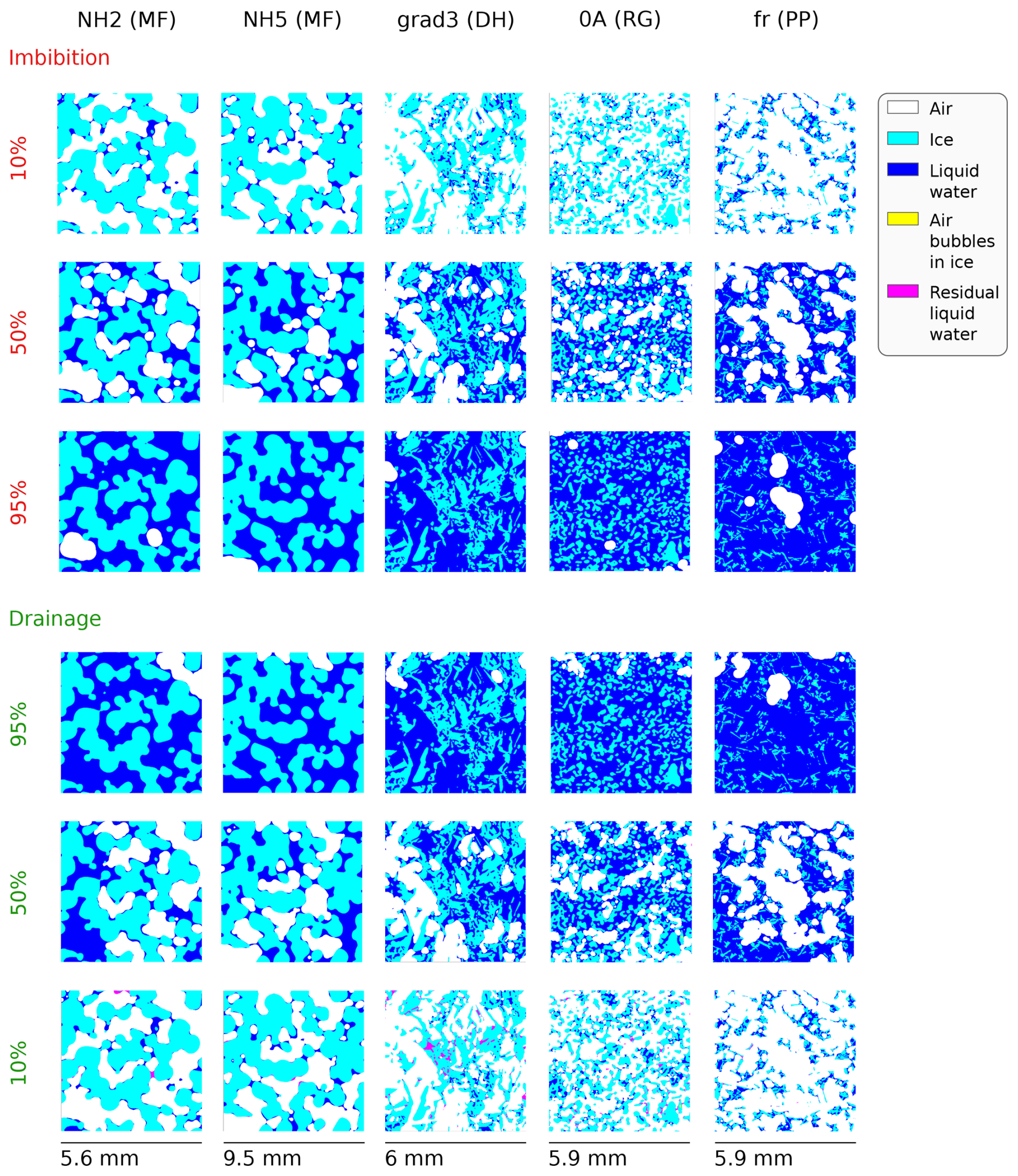
Figure 5 Vertical cross-sections of the 5 selected snow samples with drainage and imbibition processes at 3 stages of effective saturation. The cross-sections are taken in the center of the samples. The reservoir of the wetting phase is located on the bottom boundary and the reservoir of the non-wetting phase is located on the top boundary.

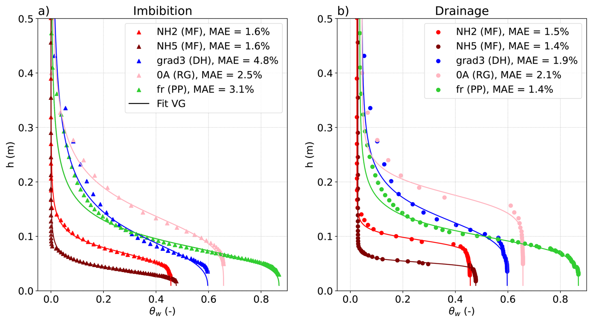
Figure 6 Numerical imbibition (a) and drainage (b) WRCs for different types of snow samples with the corresponding VG fits. The curve colors represent the different snow types. The MAEs on θ_w of the fits are expressed in percent.

Daanen and Nieber (2009)Yamaguchi et al. (2010)Yamaguchi et al. (2012)

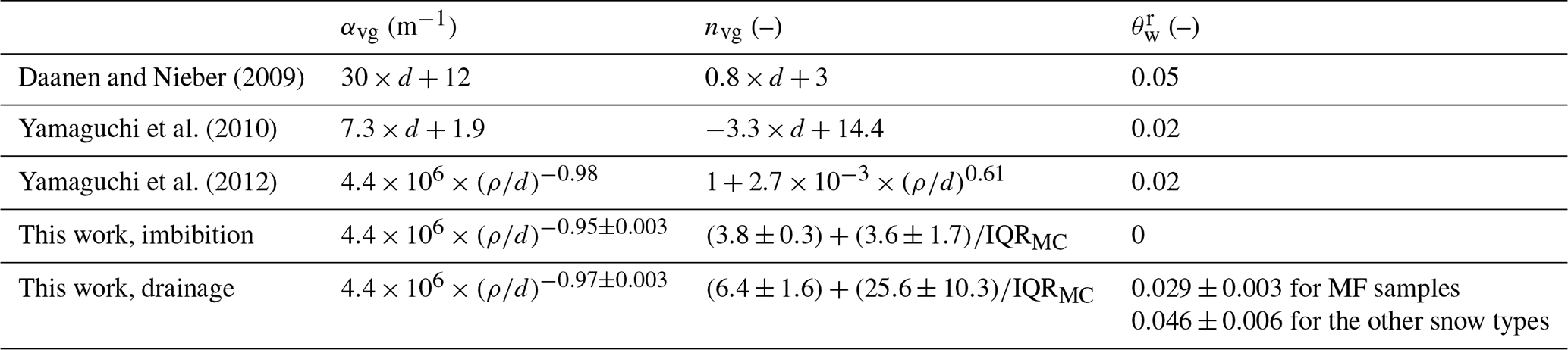
Table 2 Regressions of the shape parameters of the VG model α_vg, n_vg and ${\mathit{\theta }}_{\mathrm{w}}^{\mathrm{r}}$ proposed by Daanen and Nieber (2009), Yamaguchi et al. (2010, 2012), and from this work for both imbibition and drainage. For the derived regressions, standard deviations are given for each coefficient.

3 Results and discussion

3.1 Water retention curves

3.1.1 WRCs of different snow microstructures and their related VG fits

Figure 5 presents vertical cross-sections of the drainage and imbibition simulations at three stages of water saturation for the five selected snow samples described in Table 1. The pore-scale distribution of liquid water in the microstructures can be observed. For imbibition, the small pores are first filled, and the larger pores are filled last. For drainage, it is the other way around, with water escaping the large pore first. Residual liquid water at the end of the drainage simulation is shown in pink. Air bubbles entrapped in the ice skeleton are shown in yellow (for instance, in the bottom right of the 0A (RG) sample). This figure also highlights the fact that, for a given saturation, the liquid water distribution is different depending on the snow types, as well as between the imbibition and drainage processes.

Figure 6a and b present the WRCs of the imbibition and drainage simulations applied to the 5 selected snow samples presented in Table 1. A first result is that the WRCs of the snow samples present generally significant hysteresis, as they differ between imbibition and drainage (see also Fig. 4b). Overall, a steeper WRC is found for imbibition compared to drainage, and h values are higher for drainage compared to imbibition.

The influence of the snow geometrical properties can be observed. Snow samples presenting small grains (0.06–0.15 mm), such as the samples fr (PP), 0A (RG), and grad3 (DH), show higher pore pressures at a given water content than the samples NH2 (MF) and NH5 (MF) presenting coarse grains (0.53–0.87 mm). Snow density also has a direct influence on the WRCs, as it limits the maximum water content that can be reached. More subtly, the WRCs tend to show sharper transitions for the most evolved snow microstructures.

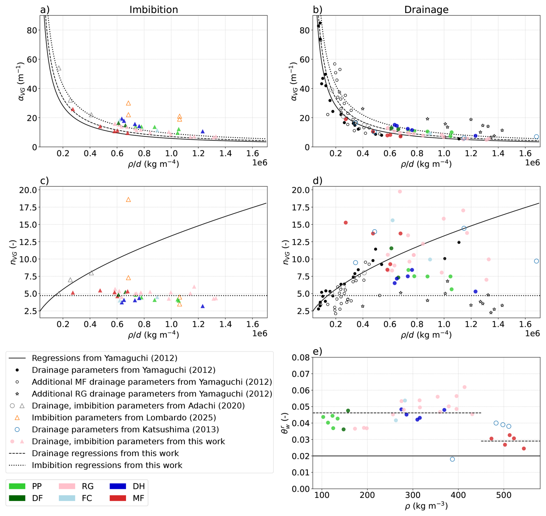
Figure 7 (a, b) α_vg, (c, d) n_vg and (e) ${\mathit{\theta }}_{\mathrm{w}}^{\mathrm{r}}$ parameters of the VG model as a function of $\mathit{\rho }/d$ or ρ for imbibition and drainage. The regressions of Yamaguchi et al. (2012) are shown by black lines, the values used to derive those regressions are shown by black disks (“S-samples”, composed of refrozen MF – see Yamaguchi et al., 2012). The additional drainage measurements from Yamaguchi et al. (2012) are shown by circles (MF samples) and stars (RG samples). Measurements from Adachi et al. (2020) are shown by empty gray markers. Measurements from Lombardo et al. (2025) and Katsushima et al. (2013) are shown by empty orange triangles and blue circles. From this work, parameters from imbibition and drainage simulations are shown by colored disks and triangles, respectively, the colors showing the snow types. The proposed regressions based on our simulated data are shown by dashed and dotted lines (see Table 2).

For each microstructure, we also present the related VG fit (Eq. 2) that best reproduces the simulated WRC. In other words, the VG parameters α_vg, n_vg, and ${\mathit{\theta }}_{\mathrm{w}}^{\mathrm{r}}$ were optimized to best fit the simulated WRC of each snow sample for imbibition and for drainage. The fitting is rated in terms of MAE (mean absolute error) on θ_w and expressed as a percentage. The fitted WRCs show overall good agreement with the simulated WRCs, as illustrated for the five selected snow samples in Fig. 6a and b. The fits show slightly better results for drainage than for imbibition, and for MF samples compared to the other snow types. The model fits the data points better in the wet part compared to the dry part for snow types such as RG and PP. This might be due to (i) the fact that $m_{\text{vg}}=\mathrm{1}-\mathrm{1}/n_{\text{vg}}$ constrains the shape of the fit, and that (ii) the data points are not evenly distributed in this θ_w, as the simulation step is the pore radius and not the water content. In future studies, the VG formulation could be refined using more parameters, such as m_vg, to enable fitting both the left and right inflection points of the WRCs, especially for drainage.

3.1.2 Analysis of the VG parameters

Figure 7 presents the VG parameters α_vg, n_vg and ${\mathit{\theta }}_{\mathrm{w}}^{\mathrm{r}}$ obtained by fitting the VG model to our simulated WRCs for all our dataset. The parameters, obtained for imbibition and drainage, are expressed as a function of the term $\mathit{\rho }/d$ or ρ, following Yamaguchi et al. (2012), and compared to the regressions suggested by Yamaguchi et al. (2012) (black solid curves in Fig. 7). In addition, the measurement data of α_vg and n_vg from Yamaguchi et al. (2012); Katsushima et al. (2013); Adachi et al. (2020) and Lombardo et al. (2025) are also shown. They correspond to values derived from WRCs obtained from laboratory experiments of imbibition and drainage. As specified in Sect. 2.2, in all our computations, d was estimated based on the SSA, following the formula $d=\mathrm{2}\times r_{\text{es}}=\mathrm{6}/(\text{SSA}\times {\mathit{\rho }}_{\mathrm{i}})$ with ρ_i =  917 kg m⁻³ the ice density.

α_vg parameter

Overall, the parameter α_vg decreases with increasing $\mathit{\rho }/d$, so when density increases and/or grain size decreases. This trend is in overall consistent with the measurements of Yamaguchi et al. (2012), Adachi et al. (2020), Katsushima et al. (2013), and Lombardo et al. (2025). Moreover, α_vg values from the imbibition simulations are systematically larger than the ones from the drainage simulations. This is in agreement with the hysteresis reported by Adachi et al. (2020) and with the high α_vg values obtained from imbibition experiments by Lombardo et al. (2025). The α_vg values from our simulations and the regression of Yamaguchi et al. (2012) are overall in good agreement for drainage, with a MAE of 25 %, a little less so for imbibition, with a MAE of 38 %.

Following the formulation of Yamaguchi et al. (2012), we proposed two new regressions of α_vg, which allow reproducing the different behaviors between imbibition and drainage. Their expressions are provided in Table 2. They are shown in Fig. 7a and b, and have a MAE of 17 % when compared to our data. The proposed regressions were derived from snow samples with $\mathit{\rho }/d$ values comprised between 0.25 × 10⁶ and 1.3 × 10⁶ kg m⁻⁴, and do not cover the lowest values of $\mathit{\rho }/d$ (< 0.25 × 10⁶ kg m⁻⁴), for which a steep evolution of α_vg was reported (Yamaguchi et al., 2012; Adachi et al., 2020). Still, we derived our regressions with an exponential form to be consistent with these observations and following Yamaguchi et al. (2012).

We use the α_vg parameter to quantify the degree of hysteresis of the WRCs, based on the ratio α_vg from imbibition over α_vg from drainage. For our set of images, this ratio ranges from 1.19 to 1.42, with an average value of 1.28. It is consistent with the ratios measured by Adachi et al. (2020), for which values of 1.46, 1.52, and 1.38 are found for the S, M, and L samples, respectively. No correlation was found between this ratio and grain type, grain size, or density. Our ratios and the ones of Adachi et al. (2020) tend to confirm hysteresis ratios around 1.5 for snow, which is lower than the classical value of 2 used for soils (Likos et al., 2013; Leroux and Pomeroy, 2017).

n_vg parameter

The results obtained from the simulations are more surprising regarding the parameter n_vg. For imbibition, the n_vg values show little variation for the whole range of $\mathit{\rho }/d$ and are around 4.7 (Fig. 7d). These results are rather consistent with the n_vg values of Lombardo et al. (2025) but not with those of Adachi et al. (2020). The latter authors report a correlation of the n_vg with $\mathit{\rho }/d$ that follows the regression of Yamaguchi et al. (2012) based on drainage experiments, not observed in our work and the one of Lombardo et al. (2025).

The n_vg values for drainage are overall much higher compared to imbibition, as opposed to the findings of Adachi et al. (2020) for snow or many soils observations (Likos et al., 2013), which mention similar values of n_vg for drainage and imbibition. Our results are more consistent with the ones of Lombardo et al. (2025) for snow or with granular materials (Cheng et al., 2012; Sweijen et al., 2016) for which n_vg values in imbibition can be much smaller than the ones in drainage.

For drainage, our n_vg values are spread and show little correlation with $\mathit{\rho }/d$. Looking at the experimental data, a large spread is also observed in Katsushima et al. (2013), Lombardo et al. (2025), and for the rounded grains samples of Yamaguchi et al. (2012). Our estimated n_vg values overall do not follow the regression of Yamaguchi et al. (2012), although the n_vg values of the melt forms samples are closer to this regression compared to the other snow types. Let us recall that Yamaguchi et al. (2012) presented a regression based on drainage experiments on sieved melt forms only (black filled dots in Fig. 7d), which was in good agreement with n_vg values estimated on other samples of natural melt forms (black circles), but in poor agreement for samples of natural rounded grains (black stars), for which n_vg appear to be independent of $\mathit{\rho }/d$. Yamaguchi et al. (2012) attributed these different behaviors between snow samples to differences in pore-size uniformity, which seems coherent with the definition of n_vg.

To test the hypothesis that n_vg could depend on the pore-size uniformity, we characterized pore size variations by using the distributions of mean curvature of the snow microstructure, which is a standard parameter used for snow (e.g. see Lesaffre et al., 1998; Brzoska et al., 1999). The mean curvature was calculated at each point on the surface of the 3D images and represented as a statistical distribution (see Flin et al., 2004, 2005; Calonne et al., 2014a; Bouvet et al., 2022, and the Supplement for additional information). Figure 8 shows n_vg as a function of the interquartile range of the mean curvature IQR_MC of each 3D snow image for both imbibition and drainage, thus describing the relationship between n_vg and the mean curvature uniformity for both processes. A trend can be observed, so that low IQR_MC values tend to be correlated to large n_vg values, following the form of an inverse function. The trend is overall similar for imbibition and drainage, with lower values for imbibition. The observed trend is consistent with the fact that, during drainage, water leaves the pores more or less all at once for snow with rather uniform pore sizes, such as melt forms (in red), as showed by very sharp WRCs and modeled by large n_vg values (see Fig. 3b). The lower limit of IQR_MC corresponds to a material with uniform pore sizes and higher values of n_vg (step function). For snow types showing large pore size variability, such as fresh snow (in light green), n_vg values are smaller, and the resulting WRC shows a smoother transition as a function of the water content, i.e., the drainage is more gradual. The same considerations apply to imbibition, while the impact is less prominent, due to the rather large snow porosity (at least greater than 0.4 for each sample of our dataset). The imbibition is thus less dependent on the local microstructure than the drainage process.

In conclusion, to estimate n_vg, our results do not support the use of the $\mathit{\rho }/d$ ratio but rather of more refined parameters, such as the mean curvature distribution (see Fig. 8 and Table 2 for the detailed regression proposed). This can be seen as a limitation for larger-scale modeling as this parameter can currently only be derived from 3D images.

${\mathit{\theta }}_{\mathrm{w}}^{\mathrm{r}}$ parameter

The last parameter required for our use of the VG model is the residual water content ${\mathit{\theta }}_{\mathrm{w}}^{\mathrm{r}}$. As already mentioned, this parameter was set to 0 for imbibition as simulations were performed on fully dry snow images, and was only determined for drainage as the minimum value of water content reached during the drainage simulations. Two distinct groups are observed (Fig 7e). Samples with density below 450 kg m⁻³ show values centered around 0.046, which slightly increase with density from about 0.036 to 0.061. Samples of melt forms with density above 450 kg m⁻³ show smaller values around 0.029, including the NH2 and NH5 samples. This division is probably due to the fact that the denser snow samples are composed of MF that show large and uniform pores compared to the other samples. The latter could be subjected to more disconnections during drainage due to the small and complex throats, resulting in higher residual water content. All the values of ${\mathit{\theta }}_{\mathrm{w}}^{\mathrm{r}}$ from our simulations are larger than the value of 0.02 proposed in Yamaguchi et al. (2012). Following our results, we propose to approximate ${\mathit{\theta }}_{\mathrm{w}}^{\mathrm{r}}$ by two constant values depending on the snow type: 0.029 for melt forms and 0.046 for the other snow types (Fig. 7 and Table 2).

${\mathit{\theta }}_{\mathrm{w}}^{\mathrm{s}}$ parameter

To complete the picture, it seems worth discussing the saturated water content ${\mathit{\theta }}_{\mathrm{w}}^{\mathrm{s}}$. This parameter is here approximated by the snow porosity ϕ, as opposed to observations from the snow imbibition and drainage experiments (Yamaguchi et al., 2012; Katsushima et al., 2013; Adachi et al., 2020) which report ${\mathit{\theta }}_{\mathrm{w}}^{\mathrm{s}}$ ranging from 0.6ϕ to 0.9ϕ with the experimental challenge of filling complex geometries with melt and freezing processes occurring during the imbibition. In porous media such as soils and sands, imbibition and drainage experiments also show a large range between 0.3ϕ to around ϕ. Low values of ${\mathit{\theta }}_{\mathrm{w}}^{\mathrm{s}}$ are either seen as underestimated due to the experimental limits linked to the challenge of filling complex geometries, or as reflecting the real physical processes at stake (e.g., Clayton, 1999; Cho et al., 2022). Therefore, two approaches are commonly used in the literature, either the approximation ${\mathit{\theta }}_{\mathrm{w}}^{\mathrm{s}}=\mathit{\varphi }$ is taken or ${\mathit{\theta }}_{\mathrm{w}}^{\mathrm{s}}$ is adjusted to experimental data. The experiments of Likos et al. (2013) and Farooq et al. (2024) have shown that having ${\mathit{\theta }}_{\mathrm{w}}^{\mathrm{s}}$ smaller than ϕ generally implies greater α_vg values, but has no significant impact on the n_vg values. For snow purposes, the actual values of the saturated water content still remain unclear and should be further investigated to refine the VG parameters.

Conclusion on the VG parameters

The regressions of Yamaguchi et al. (2012) are in good agreement with our simulations for α_vg, especially for drainage, but not for n_vg for both imbibition and drainage, and not for ${\mathit{\theta }}_{\mathrm{w}}^{\mathrm{r}}$. We recall that the regressions of Yamaguchi et al. (2012) are based on drainage experiments only and realized on a limited number of snow types, mainly composed of dense MF, which may explain some of the observed discrepancies. For α_vg, we proposed new regressions based on $\mathit{\rho }/d$ for both imbibition and drainage, for a wide range of $\mathit{\rho }/d$ values. For n_vg, a constant value was suggested for imbibition, but no estimates for drainage could be proposed using $\mathit{\rho }/d$. A parameter that captures the pore size distribution of snow, such as the interquartile range of the mean curvature, seems to be required. For ${\mathit{\theta }}_{\mathrm{w}}^{\mathrm{r}}$, two mean values were provided depending on the snow type for drainage.

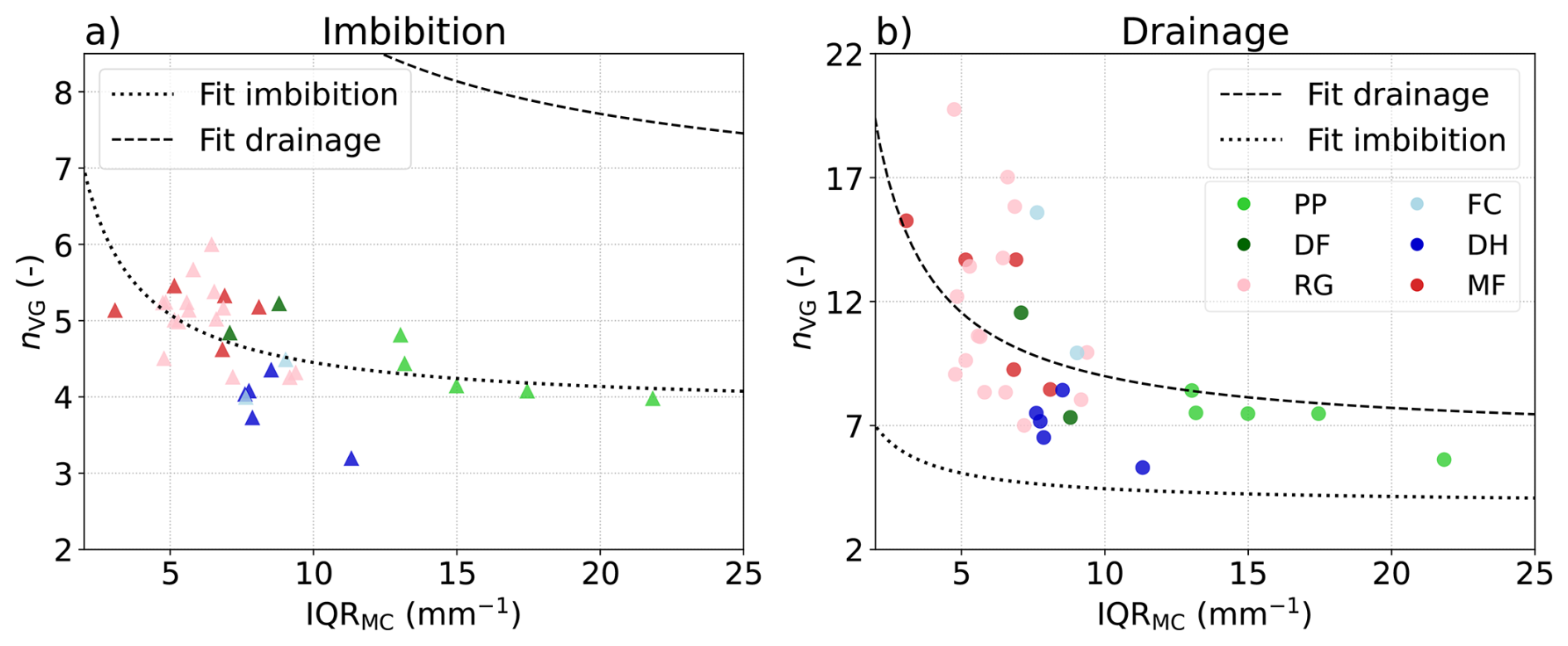
Figure 8 n_vg parameter as a function of the interquartile range IQR_MC obtained for the mean curvature distribution computed on each 3D dry snow image. Regressions for imbibition (a) and drainage (b) are shown with dotted and dashed lines (see Table 2).

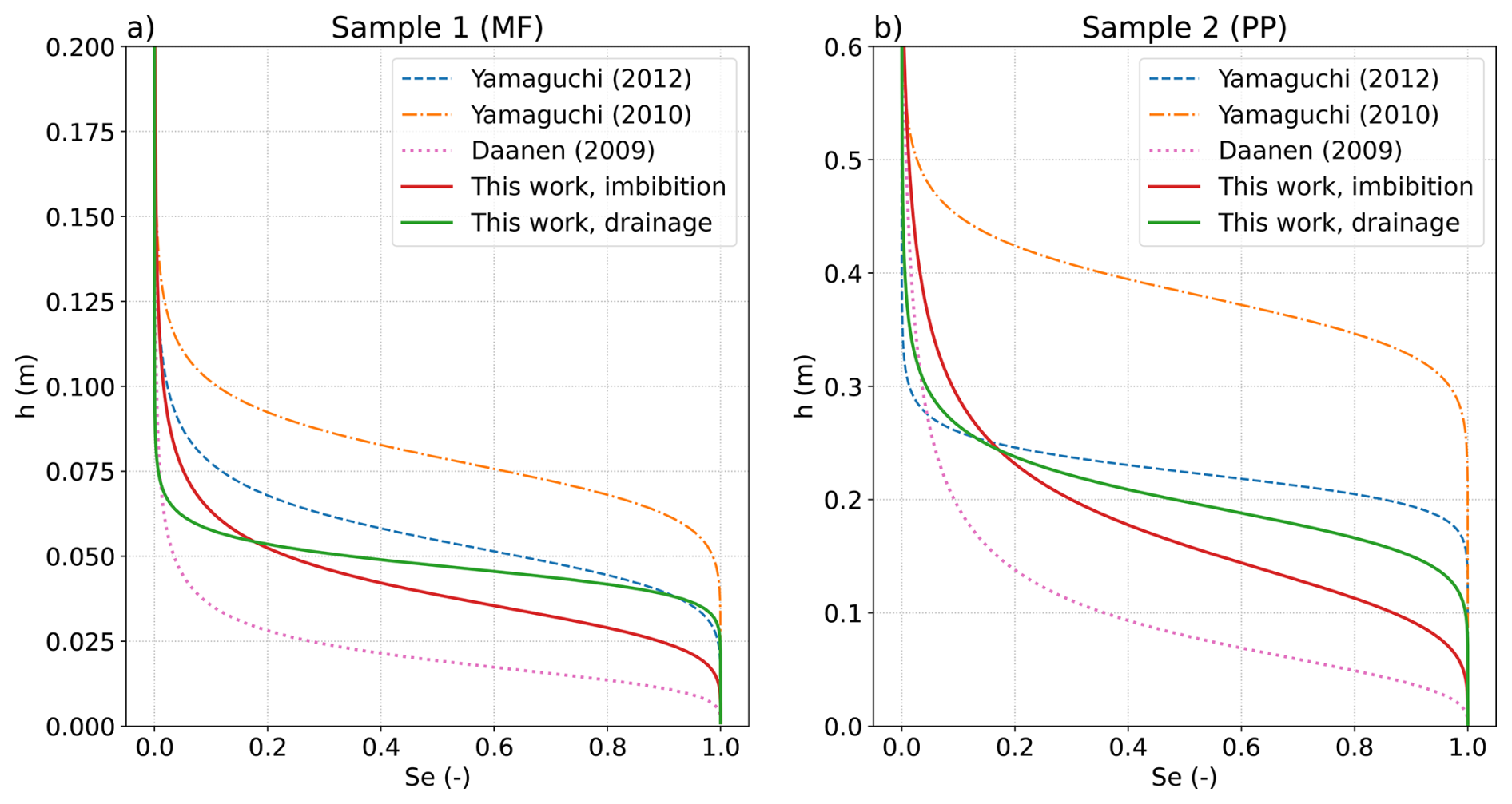
Figure 9 Illustration of the VG shape parameters regressions on the WRCs for 2 representative samples as a function of the effective saturation. The presented VG models are: imbibition and drainage models from this work and the models of Daanen and Nieber (2009), Yamaguchi et al. (2010), and Yamaguchi et al. (2012) (see Table 2).

3.1.3 Application of the different VG models on two representative snow samples

Here, we applied different VG models to predict the WRCs for drainage and imbibition for two imaginary snow samples. The properties of those samples have been chosen to be representative of melt forms (sample 1: d = 1.5 mm, ρ = 450 kg m⁻³, IQR_MC = 5 mm⁻¹) and precipitation particles (sample 2: d = 0.1 mm, ρ = 130 kg m⁻³, IQR_MC = 15 mm⁻¹). We present predictions based on the regressions of the shape parameters α_vg, n_vg, and ${\mathit{\theta }}_{\mathrm{w}}^{\mathrm{r}}$ from Yamaguchi et al. (2010), Yamaguchi et al. (2012), Daanen and Nieber (2009), and from this study for both imbibition and drainage. These regressions of the shape parameters are provided in Table 2. Daanen and Nieber (2009) and Yamaguchi et al. (2010) present a regression of α_vg and n_vg based on grain size, while Yamaguchi et al. (2012) include both grain size and snow density, using the variable $\mathit{\rho }/d$, with d the mean grain diameter. We recall that the latter three regressions have been developed based on drainage measurements only.

Figure 9 presents the WRCs for the two representative samples for the different VG models. These curves are expressed as a function of the effective saturation (e.g., Mualem, 1976; d'Amboise et al., 2017), defined in Eq. (2). Our VG models are closer to the VG model of Yamaguchi et al. (2012) for both samples, the one of Yamaguchi et al. (2010) and Daanen and Nieber (2009) being consistently above and below our estimates, respectively. Besides, the difference of WRCs estimated for imbibition and drainage on the same sample is lower than the difference between models. A larger spread of the curves can be observed for sample 2, which tends to show the highest sensitivity of the VG shape parameters for low-density and small-grain snow.

3.2 Effective wet snow transport properties

Unsaturated effective properties were computed on the simulated 3D images of wet snow obtained for different stages of the drainage simulations. We present here the results for the effective water permeability $K_{\mathrm{w}}^{\mathrm{u}}$, the effective thermal conductivity k^u, and the effective water vapor diffusivity D^u (see Sect. 2.5).

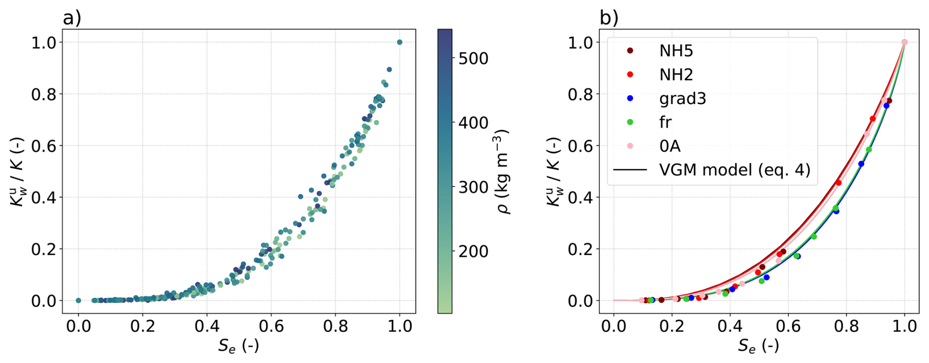
Figure 10 Effective relative water permeability as a function of the effective saturation for (a) all the snow samples, and (b) the 5 reference samples. Computations were performed on the snow images from the drainage simulations only. The dry density of the snow samples is represented by the colorbar. The VGM models of relative permeability using the shape parameters fitted on the WRC of each image (provided in the Supplement) are shown by the solid lines.

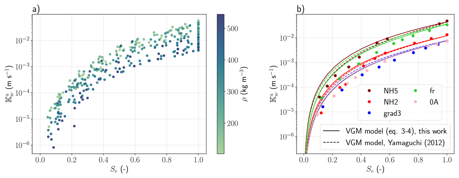
Figure 11 Unsaturated hydraulic conductivity ${\mathbb{K}}_{\mathrm{w}}^{\mathrm{u}}$ as a function of the effective saturation for (a) the whole set of snow samples, and (b) the 5 selected samples. Computations were performed on the snow images from the drainage simulations only. The dry density of the snow samples is represented by the colorbar. The VGM model, using the values of intrinsic permeability from Calonne et al. (2012) and the shape parameters from the regressions of this work given in Table 2, is shown for each sample by solid lines. The VGM model, using the values of intrinsic permeability from Calonne et al. (2012) and the regression from Yamaguchi et al. (2012) is shown with the dashed lines.

3.2.1 Water permeability and hydraulic conductivity

First, we study the effective water permeability $K_{\mathrm{w}}^{\mathrm{u}}$. To compare all the samples together, we use the relative water permeability $K_{\mathrm{w}}^{\mathrm{r}}\left({\mathit{\theta }}_{\mathrm{w}}\right)=K_{\mathrm{w}}^{\mathrm{u}}\left({\mathit{\theta }}_{\mathrm{w}}\right)/K$, with K the intrinsic permeability of the saturated media. The evolution of the relative permeability with the effective saturation is shown in Fig. 10a. The relationship describes an exponential increase, which tends, for all samples, to merge into a single curve. This shows that the water permeability is at first order driven by the water content and the snow density, and that other dependencies with other microstructural parameters are, if any, of lesser strength. We compare our results with the van Genuchten–Mualem (VGM) model of relative water permeability (Mualem, 1976), described in the introduction and in Eq. (4). For that, the shape factors of the VG model n_vg, α_vg, and $m_{\text{vg}}=\mathrm{1}-\mathrm{1}/n_{\text{vg}}$ were taken using the values fitted to the WRC of each image. In addition, the VGM model includes the parameter τ_vg, which describes the effects of the connectivity and tortuosity of the flow paths. Here we assume that ${\mathit{\tau }}_{\text{vg}}=\mathrm{1}/\mathrm{2}$, which is the default value suggested in Mualem (1976). Note that this parameter can vary depending on the porous material (e.g. Vereecken et al., 2010) and its value for snow could be refined in future works. For the 5 reference snow samples presented in Table 1, good agreements are found between the VGM model and our numerical computations (Fig. 10b).

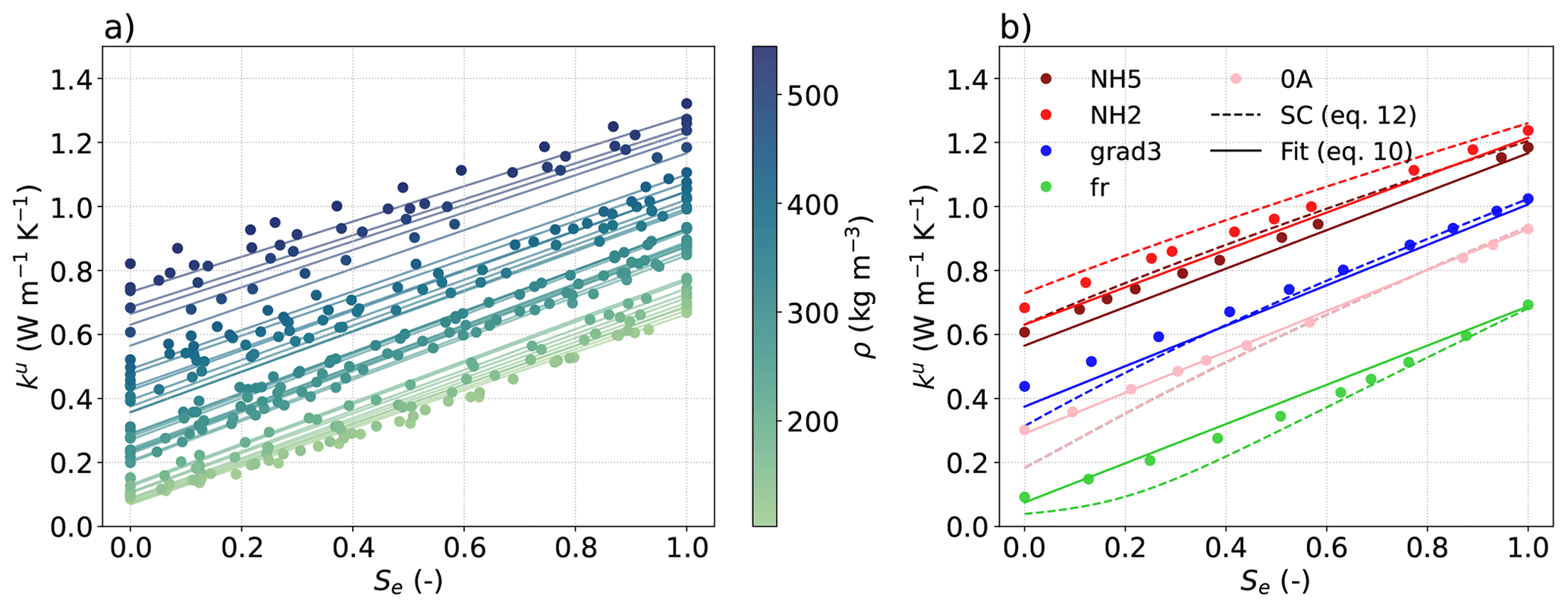
Figure 12 Unsaturated thermal conductivity k^u as a function of the effective saturation for (a) the whole set of snow samples, and (b) the 5 selected samples. Computations were performed on the snow images from the drainage simulations only. The dry density of the snow samples is represented by the colorbar. The suggested regression is shown by solid lines and the self-consistent estimate for 3 phases is shown by dashed lines.

From the relative water permeability, the unsaturated hydraulic conductivity ${\mathbb{K}}_{\mathrm{w}}^{\mathrm{u}}$ can be obtained by the following equation:

$$\begin{array}{}\text{(8)}& {\mathbb{K}}_{\mathrm{w}}^{\mathrm{u}}\left({\mathit{\theta }}_{\mathrm{w}}\right)={\mathbb{K}}_{\mathrm{w}}^{\text{sat}}\times K_{\mathrm{w}}^{\mathrm{r}}\left({\mathit{\theta }}_{\mathrm{w}}\right)\end{array}$$

with

$$\begin{array}{}\text{(9)}& {\mathbb{K}}_{\mathrm{w}}^{\text{sat}}=K{\mathit{\rho }}_{\mathrm{w}}g/{\mathit{\mu }}_{\mathrm{w}}\end{array}$$

K depends on the snow microstructure and is estimated using the parameterization of Calonne et al. (2012) based on the density and the spherical equivalent radius of snow. Figure 11 presents the unsaturated hydraulic conductivity ${\mathbb{K}}_{\mathrm{w}}^{\mathrm{u}}$ as a function of the effective saturation, showing a non-linear increase with increasing saturation. As ${\mathbb{K}}_{\mathrm{w}}^{\mathrm{u}}$ contains a K factor as compared to the relative permeability $K_{\mathrm{w}}^{\mathrm{r}}$, an effect of the microstructure can here be observed: for a given water saturation, ${\mathbb{K}}_{\mathrm{w}}^{\mathrm{u}}$ varies with density and the spherical equivalent radius, such as lighter and/or larger grain snow samples show larger ${\mathbb{K}}_{\mathrm{w}}^{\mathrm{u}}$ values (Fig 11a and b). To estimate the unsaturated hydraulic conductivity, the VGM model is here used with the shape parameters estimated from the regressions proposed in this study for drainage (given in Table 2), and combined with the parameterization of Calonne et al. (2012). The estimates are overall in good agreement with the computed data, as shown in Fig. 11b. The estimates of the unsaturated hydraulic conductivity from the VGM model using the shape parameters from Yamaguchi et al. (2012) (Table 2) are also provided for comparison (dashed lines). Both VGM models are overall fairly close. For the melt forms samples, a slight improvement is found using our regressions, with MAE values around 10 % for Yamaguchi et al. (2012) and around 9 % for our model. These similarities can be related to the fact that, on one hand, the regression of Yamaguchi et al. (2012) provides slightly better estimates of α_vg for this snow type, compared to our regression (Fig. 7b); on the other hand, n_vg values are better estimates from our regression (Figs. 7d and 8). For the other snow types, the VGM model using our shape parameter estimates provides better predictions of unsaturated hydraulic conductivity, showing MAE values around 15 % compared to the VGM model using the estimates of Yamaguchi et al. (2012), with MAEs around 22 %. Indeed, for all the snow types excluding melt forms, both shape parameters α_vg and n_vg are overall better estimated using our regression (as optimized to best match our numerical simulations). This highlights the advantage of considering a large diversity of snow to develop the regressions of the shape parameter, so that the regressions can be applied more widely. However, we point out that the VGM model based on the shape parameter estimates of Yamaguchi et al. (2012), which only required the knowledge of density and grain size, still allows for fair estimates of the unsaturated hydraulic conductivity, with MAEs ranging from 10 % to 20 %, when compared to the simulations on our five samples.

3.2.2 Thermal conductivity

The unsaturated effective thermal conductivity of wet snow k^u, which accounts for heat conduction in the ice, air, and liquid water, is presented for different saturation levels in Fig. 12. As expected, thermal conductivity increases with increasing saturation, as liquid water conducts better than air. Values of thermal conductivity of fully saturated snow are increased by about 0.5 to 0.6 $\mathrm{W}{\mathrm{m}}^{-\mathrm{1}}{\mathrm{K}}^{-\mathrm{1}}$ compared to the ones of dry snow, which means multiplying by 6 the thermal conductivity of a fresh snow sample or by 2 that of a melt form sample. The major impact of snow density is also shown, as already reported for dry snow (e.g., Sturm et al., 1997; Calonne et al., 2011). Density also influences the steepness of the linear conductivity-saturation relationship, such as dense snow shows less steep slopes than light snow. Indeed, the pore space available for a conductivity gain due to an increase in water content is smaller for denser snow. To represent the evolution of thermal conductivity with both density and liquid water content, we propose the following regression based on our data:

$$\begin{array}{}\text{(10)}& {\displaystyle }{k}^{\mathrm{u}}(\mathit{\rho },{\mathit{\theta }}_{\mathrm{w}})=k_{\text{Calonne}}^{\text{dry}}\left(\mathit{\rho }\right)+{\mathit{\theta }}_{\mathrm{w}}\left(\mathrm{1.68}\times {\mathrm{10}}^{-\mathrm{3}}\mathit{\rho }+k_{\mathrm{w}}-k_{\mathrm{a}}\right)\text{(11)}& {\displaystyle }\mathrm{\text{with }}{k}_{\text{Calonne}}^{\text{dry}}\left(\mathit{\rho }\right)=k_{\mathrm{a}}+\mathit{\rho }\left(\mathrm{2.5}\times {\mathrm{10}}^{-\mathrm{6}}\mathit{\rho }-\mathrm{1.23}\times {\mathrm{10}}^{-\mathrm{4}}\right)\end{array}$$

where $k_{\text{Calonne}}^{\text{dry}}\left(\mathit{\rho }\right)$ is the parameterization of thermal conductivity for dry snow of Calonne et al. (2011) and ρ is the dry snow density. The choice of the regression form was motivated by a concern for simplicity and to respect the two extreme cases: a volume fully made of liquid water (ρ = 0 kg m⁻³ and θ_w = 1) and a volume fully made of air (ρ = 0 kg m⁻³ and θ_w = 0). The case of a volume fully made of ice is not considered, as the regression of Calonne et al. (2011) is only valid for densities corresponding to snow (ρ≤ 550 kg m⁻³). As illustrated in Fig. 12a and b, the proposed regression reproduces well the computed data. In Fig. 12, the self-consistent (SC) estimate of thermal conductivity for a 3-phase composite aggregate of spherical inclusions (Torquato, 2005) is included for comparison. This analytical model is derived by solving the polynomial expression

$$\begin{array}{}\text{(12)}& \sum _{\mathit{\alpha }=\mathit{\{}i,a,w\mathit{\}}}{\mathit{\theta }}_{\mathit{\alpha }}{\displaystyle \frac{k_{\mathit{\alpha }}-k^{\mathrm{u}}}{k_{\mathit{\alpha }}+\mathrm{2}{k}^{\mathrm{u}}}}=\mathrm{0}\end{array}$$

where θ_α and k_α are the volume fraction and thermal conductivity of the phase α, respectively. The SC model prediction is consistent with the numerical values computed on the 3D images.

For several models of the literature, the thermal conductivity of snow as a function of the water content is needed, including snowpack models, such as the Crocus model (Vionnet et al., 2012; Lafaysse et al., 2025), or detailed models of wet snow processes, such as the one of Leroux and Pomeroy (2017). They often rely on simple approximations to include the effect of water on the effective snow thermal conductivity. In the current version of Crocus, the thermal conductivity estimate from Yen (1981) k_Yen1981, developed for dry snow, is applied to wet snow by simply accounting for the volume fraction of both ice and liquid water, as:

$$\begin{array}{}\text{(13)}& \begin{array}{rl}{k}_{\text{Crocus}}^{\mathrm{u}}(\mathit{\rho },{\mathit{\theta }}_{\mathrm{w}})& =k_{\text{Yen1981}}^{\text{dry}}(\mathit{\rho }+{\mathit{\theta }}_{\mathrm{w}}\times {\mathit{\rho }}_{\mathrm{w}})\\ & =k_{\mathrm{i}}\times {\left({\displaystyle \frac{\mathit{\rho }+{\mathit{\theta }}_{\mathrm{w}}\times {\mathit{\rho }}_{\mathrm{w}}}{{\mathit{\rho }}_{\mathrm{w}}}}\right)}^{\mathrm{1.88}}\end{array}\end{array}$$

The model of Leroux and Pomeroy (2017) relies on a weighted average of the thermal conductivity of water and of dry snow, such as:

$$\begin{array}{}\text{(14)}& k_{\text{Leroux2017}}^{\mathrm{u}}(\mathit{\rho },{\mathit{\theta }}_{\mathrm{w}})=k_{\text{Calonne}}^{\text{dry}}\left(\mathit{\rho }\right)\times (\mathrm{1}-{\mathit{\theta }}_{\mathrm{w}})+k_{\mathrm{w}}\times {\mathit{\theta }}_{\mathrm{w}}.\end{array}$$

To evaluate these two approaches, Fig. 13 presents a comparison with our data from computations and our proposed regression, for 3 snow samples. Major differences between the estimates are observed for each sample. The approximation used in Crocus largely overestimates the thermal conductivity of wet snow, up to a factor of 3 for the case of light snow at full saturation. The formulation of Leroux and Pomeroy (2017) leads overall to large underestimations compared to our data. This comparison shows that the water distribution in the pore space plays an important role in the thermal conductivity of wet snow and that considering the bulk water content only is not sufficient. This motivates further studies to improve the modeling of wet snow conductivity and test the regression proposed here.

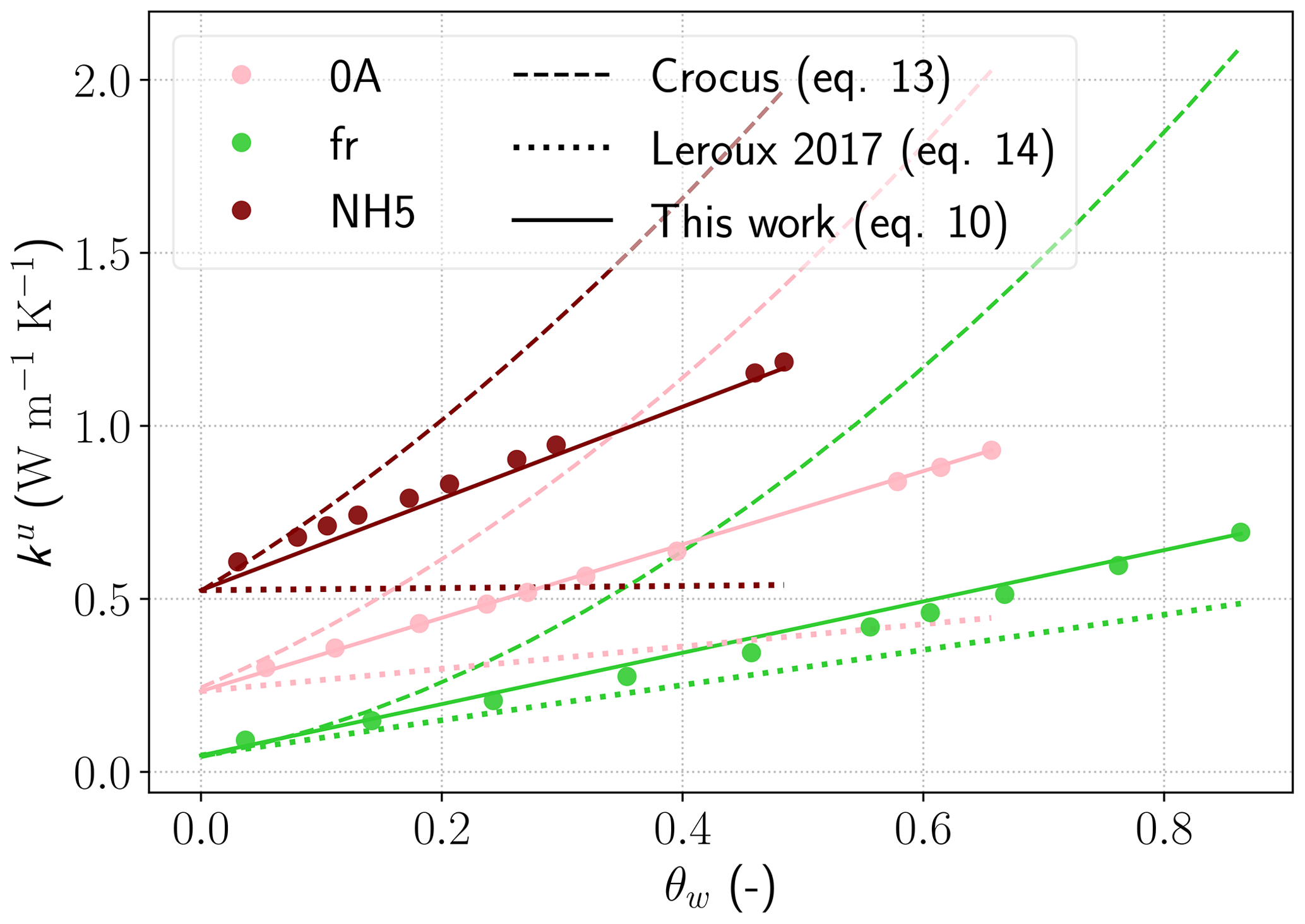
Figure 13 Comparison of the proposed regression of thermal conductivity of dry and wet snow with the regression of Crocus adapted from Yen (1981) and the one proposed by Leroux and Pomeroy (2017), for three different snow samples.

3.2.3 Water vapor diffusivity

Extending the description of water vapor diffusion of Calonne et al. (2014b) and Bouvet et al. (2024) to the wet snow problem using a similar method as for the heat transport and the liquid water flow of Moure et al. (2023), would involve the effective unsaturated water vapor diffusion D^u. As done for the water permeability, the unsaturated diffusivity D^u is normalized, here by the value of the dry effective vapor diffusivity D using the numerical estimate from Calonne et al. (2014b).

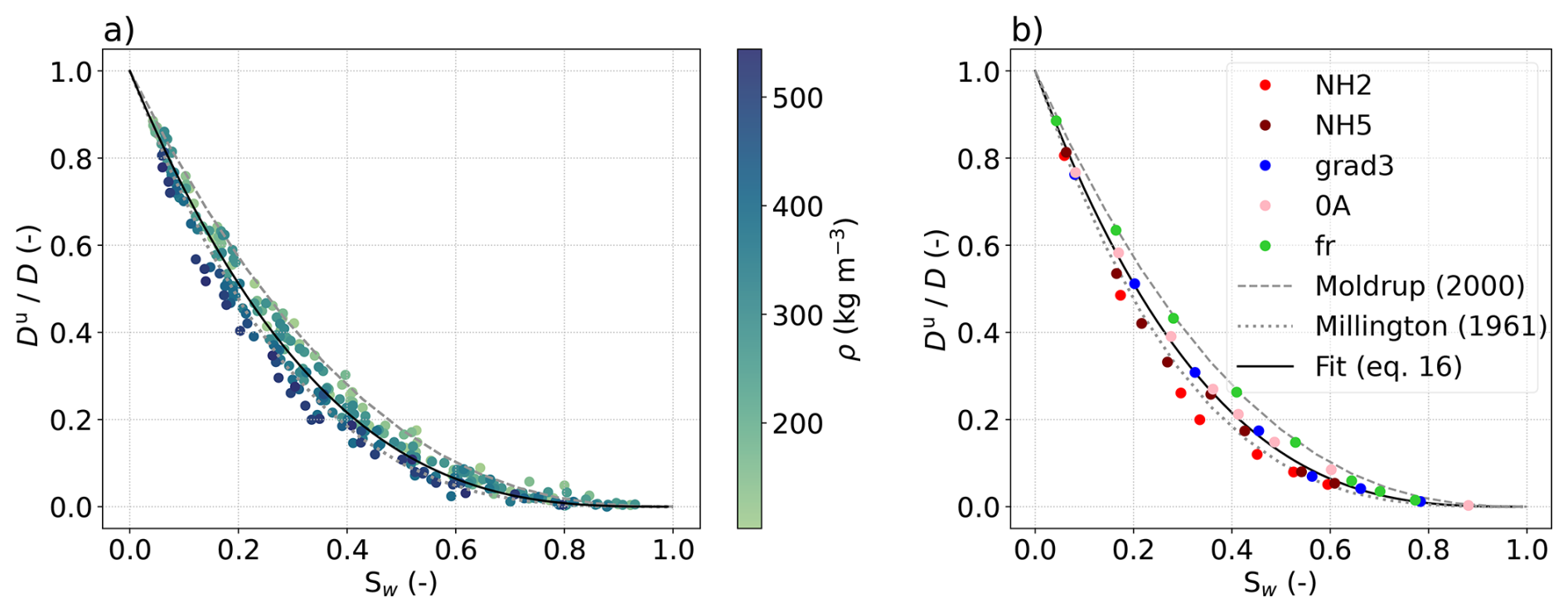
Figure 14 Relative water vapor diffusivity $D^{\mathrm{u}}/D$ as a function of the liquid water saturation S_w for drainage simulations of (a) the whole set of snow samples and (b) the 5 selected samples. The dry density of the snow samples is given by the colorbar. The proposed regression of unsaturated diffusivity is shown by a black solid line, and the models of Millington and Quirk (1961) and Moldrup et al. (2000) are shown with gray dotted and dashed lines, respectively.

Figure 14 shows $D^{\mathrm{u}}/D$ as a function of the water saturation $S_{\mathrm{w}}={\mathit{\theta }}_{\mathrm{w}}/\mathit{\varphi }$, with ϕ the porosity of dry snow. Very similar evolutions of the relative unsaturated water vapor diffusivity with the term ${\mathit{\theta }}_{\mathrm{w}}/\mathit{\varphi }$ are shown by all the samples, which highlights the strong correlation of the unsaturated diffusivity with both porosity and liquid water content. Diffusivity decreases exponentially as the proportion of liquid water increases, and for a given proportion of liquid water, diffusivity is higher for low-density snow, and inversely. Looking now at the maximum value of ${\mathit{\theta }}_{\mathrm{w}}/\mathit{\varphi }$ reached for each sample, we observe that this value varies, as suggested by Fig. 14b. The domain of definition of D^u as a function of ${\mathit{\theta }}_{\mathrm{w}}/\mathit{\varphi }$ is determined by the value of water content at which the pore space is obstructed by liquid water, and so when D^u can no longer be estimated. This specific value of water content is referred to here as the closed pore water content ${\mathit{\theta }}_{\mathrm{w}}^{\text{CP}}$. It is similar to the close-off density at which the air can no longer diffuse in the pore space, as used in Calonne et al. (2022) for dry snow and firn samples. Values of ${\mathit{\theta }}_{\mathrm{w}}^{\text{CP}}$ for all our snow samples are presented as a function of the dry porosity in Fig. 15. The closed pore water content ${\mathit{\theta }}_{\mathrm{w}}^{\text{CP}}$ is significantly smaller than the dry porosity, on average 17 % smaller. This means that vapor diffusion in wet snow is no longer possible long before saturation is reached. ${\mathit{\theta }}_{\mathrm{w}}^{\text{CP}}$ increases with increasing porosity (decreasing density), but does not seem specifically impacted by the type of snow considered. A fit, shown in black in Fig. 15, is estimated here as:

$$\begin{array}{}\text{(15)}& {\mathit{\theta }}_{\mathrm{w}}^{\text{CP}}=\mathit{\varphi }-\mathrm{0.17}\end{array}$$

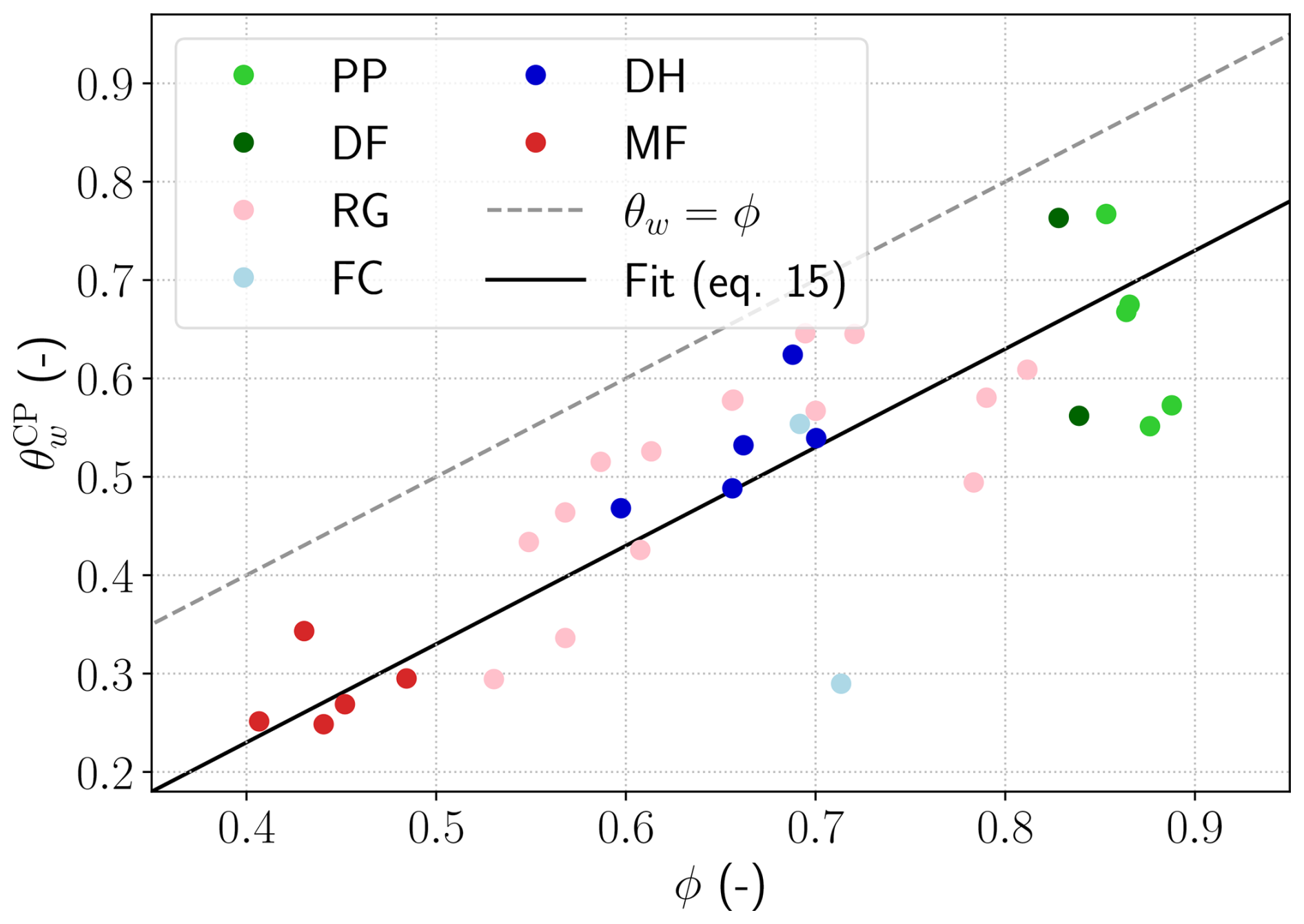
Figure 15 Values of the closed pore water content ${\mathit{\theta }}_{\mathrm{w}}^{\text{CP}}$ as a function of the snow porosity (circles). The colors represent the snow types. The saturation line θ_w=ϕ is represented with a dashed gray line and the proposed fit is shown with a solid black line.

Based on our data, a simple regression is proposed to estimate D^u from the liquid water content and the dry snow porosity:

$$\begin{array}{}\text{(16)}& {\displaystyle }\begin{array}{rl}& D^{\mathrm{u}}(\mathit{\varphi },{\mathit{\theta }}_{\mathrm{w}})=\\ & \left\{\begin{array}{l}{D}_{\text{SC}}\times {\left(\mathrm{1}-\frac{{\mathit{\theta }}_{\mathrm{w}}}{\mathit{\varphi }}\right)}^{\mathrm{3}}=D_{\text{SC}}\times {\left(\mathrm{1}-\frac{{\mathit{\theta }}_{\mathrm{w}}}{\mathrm{1}-\mathit{\rho }/{\mathit{\rho }}_{\mathrm{i}}}\right)}^{\mathrm{3}}{\mathit{\theta }}_{\mathrm{w}}\le {\mathit{\theta }}_{\mathrm{w}}^{\text{CP}}\\ \mathrm{0}{\mathit{\theta }}_{\mathrm{w}}>{\mathit{\theta }}_{\mathrm{w}}^{\text{CP}}\end{array}\right.\end{array}\text{(17)}& {\displaystyle }{D}_{\text{SC}}=D_v(\mathrm{3}\mathit{\varphi }-\mathrm{1})/\mathrm{2}\end{array}$$

with D_SC the self-consistent estimate of effective vapor diffusivity as used in Calonne et al. (2014b). This relationship follows the general form of estimates of $D^{\mathrm{u}}/D_{\text{dry}}=(\mathrm{1}-{\mathit{\theta }}_{\mathrm{w}}/\mathit{\varphi }{)}^a$ classically used for soils (Kristensen et al., 2010) with $a=\mathrm{10}/\mathrm{3}$ in Millington and Quirk (1961) and $a=\mathrm{5}/\mathrm{2}$ in Moldrup et al. (2000). The regression is shown in Fig. 14 by the black line, along with the soil models of Millington and Quirk (1961) and Moldrup et al. (2000) that are displayed with gray dotted and dashed lines. The latter two models fairly represent the behavior of D^u and bound the regression for snow with higher and lower values. Both are used for predicting D^u in structureless natural soils.

3.2.4 Sum up on the effective properties

The analysis of the effective properties based on the images obtained from the drainage simulations showed interesting results. As already mentioned, it should be kept in mind that many of these images are likely far from natural snow microstructures, as the ice structures remain unchanged in the presence of liquid water in the simulations. Yet, they offer new insights on how the liquid water distribution in snow could influence the effective transport properties for a variety of microstructures. They also enable a comparison between the current parameterizations of the transport properties and suggestions for new estimates. Especially, we showed that the classic VGM parameterization for the relative water permeability and the unsaturated hydraulic conductivity reproduces well our simulated data and seems thus a good choice for both properties. For the effective unsaturated vapor diffusivity and the effective unsaturated thermal conductivity, we proposed new regressions, which, for the conductivity, differ strongly from some of the current parameterizations used in snow modeling. Finally, as all the above effective properties were computed on images from drainage simulations only, it could be interesting to compare those estimates to the imbibition case.

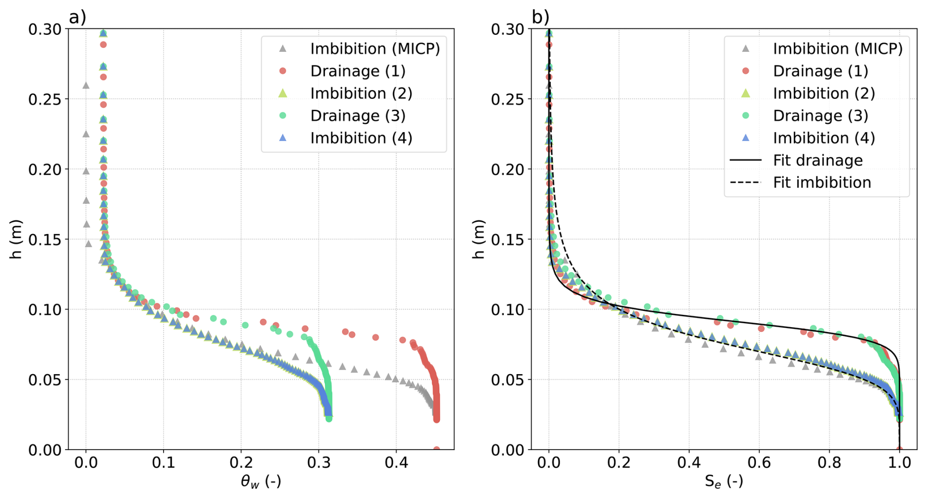
Figure 16 Example of two hysteresis cycles applied to the sample NH2, with primary drainage (1), primary imbibition (2), secondary drainage (3), and secondary imbibition (4). The boundary conditions enable entrapped residual air during imbibition and residual water during drainage. The gray points represent a first imbibition with no entrapped air enabled (MICP). (a) Liquid pressure head as a function of the water content. (b) Liquid pressure head as a function of the effective saturation. The solid and dashed black lines represent the fitted VG models used in this paper for drainage and imbibition, respectively, as provided in Table 2.

4 Main limitations

The proposed study presents different limitations:

• In the present work, the Pore Morphology Method (PMM) has been used. This method is valid in a quasi-static regime, and when capillary forces dominate in comparison to gravity and viscous forces. Dynamic effects that can occur in practice cannot be captured as in two phase flow simulations (Vogel et al., 2005; Ahrenholz et al., 2008; Bhatta et al., 2024; Prodanović and Bryant, 2006; Jettestuen et al., 2013) or using a Pore Network Model (PNM) (Vogel et al., 2005; Joekar-Niasar and Hassanizadeh, 2012; Xiong et al., 2016). Despite such limitations, the PMM provides good estimations of the WRCs for porous media whose wetting phase shows generally spherical menisci, which is the case for snow (Hilpert and Miller, 2001; Vogel et al., 2005).

• As it has already been underlined, the boundary conditions applied on the four sides of the 3D images not linked to the WP or NWP reservoir may play an important role for the residuals after drainage or imbibition. While little influence was reported for the case of drainage, the amount of residual air (or entrapped air) during imbibition may vary significantly depending on the chosen boundary conditions (see Sect. 2.3). This point, which concerns all the methods (PMM, etc.) to describe two-phase flows, has been little discussed in the literature, except in Galindo-Torres et al. (2016) and Zhang et al. (2025) in the case of lattice Boltzmann simulations. For our snow samples, preliminary tests showed that the maximum water saturation (${\mathit{\theta }}_{\mathrm{w}}^{\mathrm{s}}$) ranges from 45 % to 90 % of the porosity, depending on the applied boundary conditions (symmetry, wall, or displaced fluid outlet). More generally, knowledge on the residual air in snow seems limited. Estimates based on measurements remain an experimental challenge and show large differences (Yamaguchi et al., 2012; Katsushima et al., 2013; Adachi et al., 2020). Further work would be required to validate the proposed approach through refined comparisons with experimental data, for example, with imbibition experiments that combine measurements of the microstructure by X-ray tomography and measurements of liquid water content by neutron radiography (see e.g., Tengattini et al., 2020). At this stage, given the uncertainty, the imbibition curve was simulated assuming that there is no air residuals, as in the Mercury Injection Capillary Pressure (MICP) experiments (e.g. Hilpert and Miller, 2001; Berg et al., 2016), thus ${\mathit{\theta }}_{\mathrm{w}}^{\mathrm{s}}=\mathit{\varphi }$. Figure 16 presents a comparison of the WRCs with and without taking into account entrapped air during imbibition for the sample NH2. Hysteretic cycles were applied with boundary conditions (displaced fluid outlet) applied on the 4 faces of the volume not linked to the reservoirs, enabling residual air during imbibition and residual water during drainage. For these hysteretic cycles, the sample is initially fully saturated, then the sample is submitted to drainage, imbibition, drainage, and imbibition. Fig. 16a shows the WRCs of each of these steps (Drainage (1), Imbibition (2), Drainage (3), and Imbibition (4)) as a function of the water content, as well as the WRC of imbibition assuming no air residuals (MICP). We can observe that, at the end of Imbibition (1) and (2), the residual air content is about 0.14, so the water saturation does not exceed 70 %. As mentioned, this value can vary depending on the boundary conditions applied to the 4 lateral faces of the volume. Fig. 16b shows the same data as Fig. 16a, but with respect to the effective saturation. The continuous lines represent the fitted VG model proposed in this study, with the shape parameters from Table 2, so derived from our simulated WRCs of drainage and of imbibition without entrapped air. These two fitted VG models provide a good description of the entire drainage-imbibition process, regardless of whether air residuals are accounted for or not. Indeed, entrapped air has almost no impact on the value of n_vg, and a slight impact of around 10 % on the value of α_vg. A similar conclusion was reported in the experiments of Likos et al. (2013) and Farooq et al. (2024) for soils, which showed that having ${\mathit{\theta }}_{\mathrm{w}}^{\mathrm{s}}$ smaller than ϕ generally implies greater α_vg values, but has no significant impact on the n_vg values.

• Since the PMM is applied to 3D images, uncertainties can arise from the size and resolution of the images under consideration. The effects of both parameters on the results are available in Hilpert and Miller (2001) and Vogel et al. (2005), and are assumed to be transferable to snow. In the present study, we checked that our snow images correspond to representative elementary volumes. Uncertainties remain regarding the side length of the melt forms images, for which the maximum available sizes were taken, but they still present a limited number of heterogeneities.

• Our simulated WRCs were compared to WRCs measured during experiments of drainage and or imbibition. Such a comparison is not straightforward, as, in the experiments, the snow microstructure can evolve rapidly when in contact with liquid water, whereas, in the simulations, the ice skeleton is fixed and defined by the provided tomography image, always remaining in its initial stage. The comparison simulation-experiment was mainly done through the comparison of the shape parameters of the VG model derived from the WRCs. Experimental estimates remain, however, limited, often focusing either on imbibition or on drainage, or studying only a small range of snow types (Yamaguchi et al., 2010, 2012; Katsushima et al., 2013; Adachi et al., 2020; Lombardo et al., 2025). While estimates of α_vg are rather consistent between all the measurements and our simulations for both imbibition and drainage (Fig. 7a and b), estimates of n_vg differ significantly (Fig. 7c and d). Hence, it is difficult to conclude on the evaluation of our simulations. Again, dedicated studies would be required to provide further experimental data.

• Finally, the uncertainties of the WRCs simulations are not necessarily transferred to the estimates of the effective transport properties of wet snow. The simulations provide the 3D skeleton of the air, ice, and liquid water, for which the distribution of each phase in space can contain errors, as discussed above. However, only the model of unsaturated hydraulic conductivity required both the volumetric fractions and the 3D distribution of the phases through the shape factors of the WRCs (α_vg and n_vg). In contrast, the estimations of unsaturated thermal conductivity and water vapor diffusivity of snow depend on the volumetric fraction of the phases and not on the shape factors (see Eqs. 10 and 16).

5 Conclusion

In this study, a Pore Morphology Model (PMM) was used to simulate the distribution of liquid water in the pore space of snow for various water contents. Liquid water was gradually introduced and then removed by capillarity during wetting (imbibition) and drying (drainage) simulations. This model was applied to a set of 34 3D tomography images of dry snow presenting various microstructures. For each dry snow image, a series of 3D images of wet snow at different stages of imbibition or drainage was produced. Unlike what happens in nature, the ice matrix is fixed and does not evolve with the liquid water in the simulations (no wet snow metamorphism). The simulations were performed with a saturation water content set to the porosity value (no air residuals). This work constitutes an exploratory numerical work to study (i) the water retention curves (WRCs) of snow and (ii) the effective transport properties of wet snow, notably how they are influenced by the water distribution at the pore scale. Both points are critical to better understand and model water flow, heat, and vapor transport in wet snow (e.g., Leroux and Pomeroy, 2017; Moure et al., 2023).

The WRCs of snow were derived from the simulated wet snow images, for both imbibition and drainage. We confirm the hysteresis of both processes and highlight the dependency of the WRC on the microstructural features of snow, such as the snow density and interfacial mean curvature distribution. We then reproduced our WRCs with the model of van Genuchten (1980) and derived new values of the model parameters, which are the shape parameters α_vg and n_vg and the residual water content ${\mathit{\theta }}_{\mathrm{w}}^{\mathrm{r}}$ (the saturated water content ${\mathit{\theta }}_{\mathrm{w}}^{\mathrm{s}}$ being set to the porosity value in our study). Comparing with values from previous experimental studies (Yamaguchi et al., 2012; Katsushima et al., 2013; Adachi et al., 2020; Lombardo et al., 2025), we point out an overall fair agreement for α_vg but significant differences for n_vg and ${\mathit{\theta }}_{\mathrm{w}}^{\mathrm{r}}$, even between the experimental literature values themselves. Possible causes of these discrepancies are discussed. We propose new parameterizations of α_vg, n_vg, and ${\mathit{\theta }}_{\mathrm{w}}^{\mathrm{r}}$, for both imbibition and drainage processes, optimized for our simulated WRCs. They should contribute to a more generalized use of this model to predict the WRCs of snow, as needed for water flow modeling. Dedicated investigations should, however, be performed to further evaluate those parameterizations, especially concerning the exact values of the saturated water content ${\mathit{\theta }}_{\mathrm{w}}^{\mathrm{s}}$, which remains an open question.

Effective transport properties of wet snow were then estimated based on the series of images from the drainage simulations. They include the unsaturated hydraulic conductivity, water permeability, thermal conductivity, and water vapor diffusivity. These properties were computed using the Geodict software, solving boundary problems resulting from the homogenization process applied to the heat, vapor, and water transport equations. We describe the relationships of the transport properties depending on water content and dry snow density. We show that the relative water permeability and the unsaturated hydraulic conductivity can be well reproduced by the VGM model (Mualem, 1976; van Genuchten, 1980), combined with the estimates of intrinsic permeability for dry snow of Calonne et al. (2012). For the effective thermal conductivity, we report large discrepancies between our numerical results and some current estimates used in snow models, such as the Crocus model (Vionnet et al., 2012; Lafaysse et al., 2025) or the model of Leroux and Pomeroy (2017). A new parametrization based on both snow density and water content was suggested. Finally, a regression was proposed for the first time to predict the water vapor diffusivity of wet snow, which relies on the dry snow diffusivity estimated from the self-consistent model, the water content, and the snow density. This regression is close to vapor diffusivity parameterizations used for soils (Millington and Quirk, 1961; Moldrup et al., 2000).

Results of this study are a first step toward a better characterization of the distribution of liquid water in the pore space of snow, as well as a better modeling of the physical properties of wet snow. Future studies will take into account additional processes, such as the transformation of the microstructure by phase changes and the movement of water by gravity.