Ensemble numerical simulation of permafrost thermal regimes over the Tibetan Plateau using the Flexible Permafrost Model: 1950–2023

Permafrost is a subsurface phenomenon that is difficult to be measured directly, and understanding its dynamics as well as influences under a warming climate depends critically on numerical simulations. However, this task presents significant challenges as the state-of-the-art land surface models are weak in their ability to represent permafrost processes. In this study, we introduce a new land surface scheme specifically designed for permafrost applications, the Flexible Permafrost Model (FPM). This model serves as an adaptable framework for implementing innovative parameterizations of permafrost-related physics. The FPM accounts for heat flow at and below the soil surface, while simultaneously resolving the land-atmosphere energy exchanges through comprehensive treatment of radiative balance and turbulent flux dynamics. We simulate the ground thermal regime and test the model with a network of permafrost measurements across the Tibetan Plateau.

Our result yields root mean square error values of 1.0 m for active layer thickness and 1.0 °C for the mean annual ground temperature at 15 m depth of permafrost. We estimate that the current extent of permafrost (2010–2023) on the Tibetan Plateau is approximately $\mathrm{1.07}\pm \mathrm{0.02}\times {\mathrm{10}}^{\mathrm{6}}$ km². Long-term simulations indicate that the permafrost temperature increased at a rate of 0.11 °C per decade since 1980 with a decreased area of 14.6×10⁴ km² (∼12.4 %). These ensemble simulations provide valuable information on the dynamics of permafrost over the Tibetan Plateau. Furthermore, our findings suggest that current land surface models, which utilize shallow soil columns (typically ∼3 m), are insufficient for permafrost simulations over the Tibetan Plateau due to the typically deep active layer (that is, 2.68±0.82 m by mean) and may not be suitable for future projections.

1 Introduction

Permafrost regions occupy more than one-fifth of the exposed land area in the Northern Hemisphere (Gruber, 2012). Long-term records revealed steady warming of permafrost over the past several decades at a global scale (Biskaborn et al., 2019). This has led to significant degradation of the permafrost, such as a deepening active layer (Cao et al., 2018; Biskaborn et al., 2019), decreased permafrost area (Chadburn et al., 2017; Sun et al., 2022; Langer et al., 2024), expanded thermokarst (Wellman et al., 2013; Chen et al., 2021), and potential carbon decomposition (Schuur et al., 2015). Permafrost degradation has considerable influences on ecosystems, hydrological systems, and the integrity of the infrastructure (Hjort et al., 2018; Walvoord et al., 2019; Schuur and Mack, 2018). Therefore, detailed investigations of changes in permafrost in response to a warming climate are crucial for sustainable management and adaptation strategies.

Despite permafrost's importance, direct permafrost measurements, such as borehole temperature, are rare due to harsh environments and high costs (Biskaborn et al., 2015). This is especially true on the Tibetan Plateau (TP), where complex terrain and high altitudes impose further constraints on permafrost research (Cao et al., 2017b, 2019b). For these reasons, there is often a lack of essential in situ information to develop suitable statistical models (Zhao et al., 2021; Cao et al., 2021). Therefore, process-based simulation is an increasingly important tool for transient assessment of permafrost conditions and dynamics.

The TP, also known as the Third Pole, has the largest extent of permafrost in the low-middle latitudes (Cao et al., 2019b). Significant efforts have been made to understand the permafrost changes over the TP based on simulations. A large portion of these contributions comes from the hydrological community, employing models originally designed to simulate hydrological processes in permafrost-affected regions. Many of the models implemented detailed representations of hydrological processes (e.g. water mass balance) while simplifying the surface energy balance and soil thermal processes. For instance, the DHTC model parameterized ground heat conduction as a linear function of net radiation (Guo et al., 2024), and the FLEXTopo-FS model uses the empirical method (i.e. Stefan equation) for freeze/thaw processes (Gao et al., 2022). In addition to such hydrological models, the process-based models used for recent transient permafrost simulation over the TP can be generally divided into geothermal numerical models (i.e. GIPL model) and the common land surface models (i.e. CLM and Noah-MP). The geothermal numerical models typically have rich permafrost-specific processes, such as suitable numerical solver in heat transfer with soil phase changes (Nicolsky et al., 2007; Tubini et al., 2021), deep soil column (tens to hundreds of meters), and well-defined lower boundary, but lack representation of land-atmosphere interactions (i.e. Qin et al., 2017a; Sun et al., 2023). On the other hand, the land surface models benefits from the consideration of land-atmosphere processes, and therefore outperform in describing the responses of permafrost to climate warming (i.e. Guo et al., 2018; Wu et al., 2018; Zhang et al., 2021; Cao et al., 2022).

Recently, several permafrost-specific land surface schemes have been proposed to integrate the strengths of both model types. The stand-alone models yield promising potential for application to cross-scale permafrost processes (Fiddes et al., 2015; Westermann et al., 2016). However, dedicated stand-alone permafrost models remain scarce for the TP. Most existing simulations rely on distributed hydrological models, such as GBEHM and WEB-DHM, that have been enhanced with permafrost process representations (e.g. Qin et al., 2017b; Gao et al., 2018; Song et al., 2020). Although these models generally offer more realistic and detailed simulations of permafrost-influenced hydrological processes, they are typically confined to site or regional scales and short time periods due to their demand for extensive spatial data and high computational cost (i.e. Pan et al., 2016; Zhang et al., 2017; Zheng et al., 2020).

In this study, we introduce a new land surface scheme specifically designed for permafrost applications, the Flexible Permafrost Model (FPM). This model serves as a flexible platform for a variety of permafrost processes. The suitability of the new model was carefully evaluated, we then employed it in analyzing the long-term (1950–2023) permafrost thermal regime over the TP based on the ensemble simulation. Specifically, this study

• 1.

  gives a detailed description of the model conceptualization, structure, and key parameterizations;

• 2.

  evaluates the model performance in reproducing permafrost characteristics based on the ensemble approach, such as active layer thickness (ALT), and the thermal state;

• 3.

  interprets current conditions and historical changes of permafrost in response to climate change from the stand-alone simulations;

• 4.

  proposes insights for future model developments.

2 Flexible Permafrost Model (FPM)

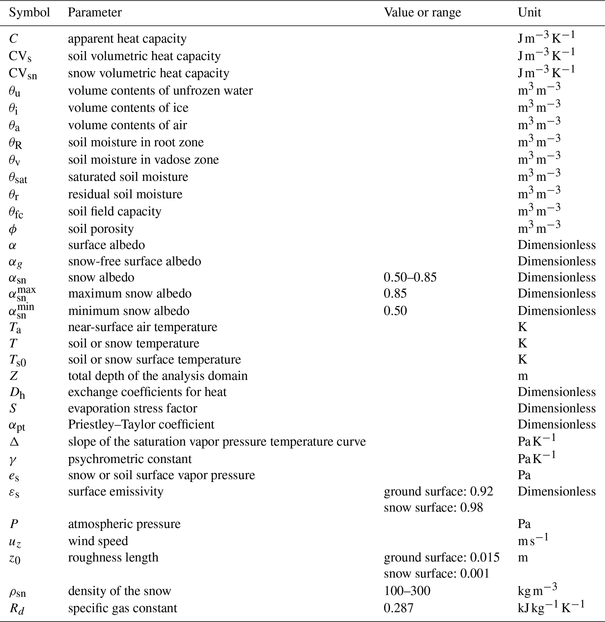
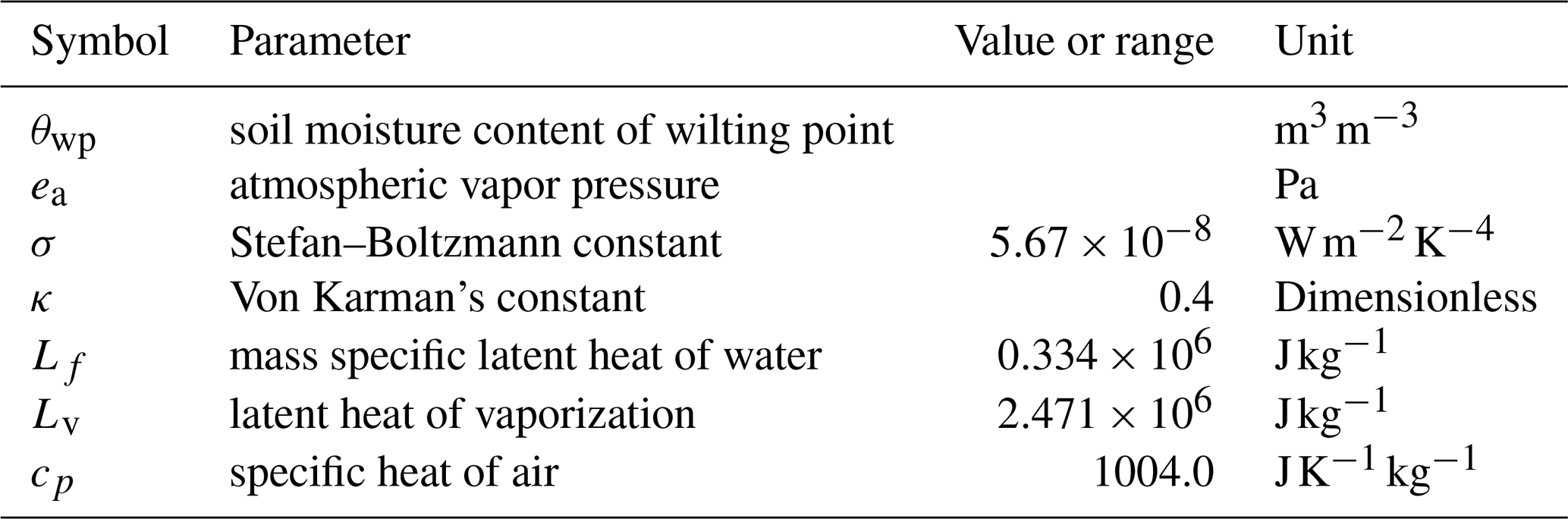
FPM accounts for heat flow with phase change at and below the soil surface, while also describing the energy exchange with the atmosphere by considering radiative and turbulent fluxes. In this study, we give the detailed introduction and evaluation of FPM and employ it in analyzing large-scale permafrost studies. The nomenclature of key model parameters are given in Table 1, and constants are in Table B1.

Table 1 Nomenclature and input parameters in Flexible Permafrost Model (FPM).

2.1 Surface energy balance

The soil or snow surface temperature (T_S0, K) was treated as upper boundary of the soil column. To derive T_S0, a physically-based surface energy balance scheme for different land surface cover types was coupled to FPM, and was formulated as:

$$\begin{array}{}\text{(1)}& {\displaystyle }{\displaystyle }\left(\mathrm{1}-\mathit{\alpha }\right)Q_{\text{si}}+Q_{\text{li}}+Q_{\text{le}}+Q_{\mathrm{h}}+Q_{\mathrm{e}}=Q_{\mathrm{c}}\end{array}$$

where Q_si is the incoming shortwave radiation, Q_li is the incoming longwave radiation, Q_le is the emitted longwave radiation, Q_h is the turbulent exchange of sensible heat, Q_e is the turbulent exchange of latent heat, and Q_c is the energy transport due to conduction. All the above energy terms have units of W m⁻². The α (–) is the surface albedo, obtained as a fraction-weighted average of albedo from snow-free (α_g) and snow-covered (α_sn) areas.

$$\begin{array}{}\text{(2)}& {\displaystyle }{\displaystyle }\mathit{\alpha }=(\mathrm{1}-\text{SCF})\cdot {\mathit{\alpha }}_g+\text{SCF}\cdot {\mathit{\alpha }}_{\text{sn}}\end{array}$$

where SCF (–) is the snow cover fraction (see Sect. 2.2), and α_g is from MODIS products whenever snow is not present (Table 2).

Muñoz-Sabater et al. (2021)Moesinger et al. (2020)Myneni et al. (2021)Su et al. (2019)Jia et al. (2022)H SAF (2020)Parinussa et al. (2015)Dorigo et al. (2017)Fernandez-Moran et al. (2017)O'Neill et al. (2021)Dai et al. (2019)Shangguan et al. (2017)Fan et al. (2013)Davies (2013)

Table 2 Climate forcing and input datasets used in Flexible Permafrost Model (FPM).

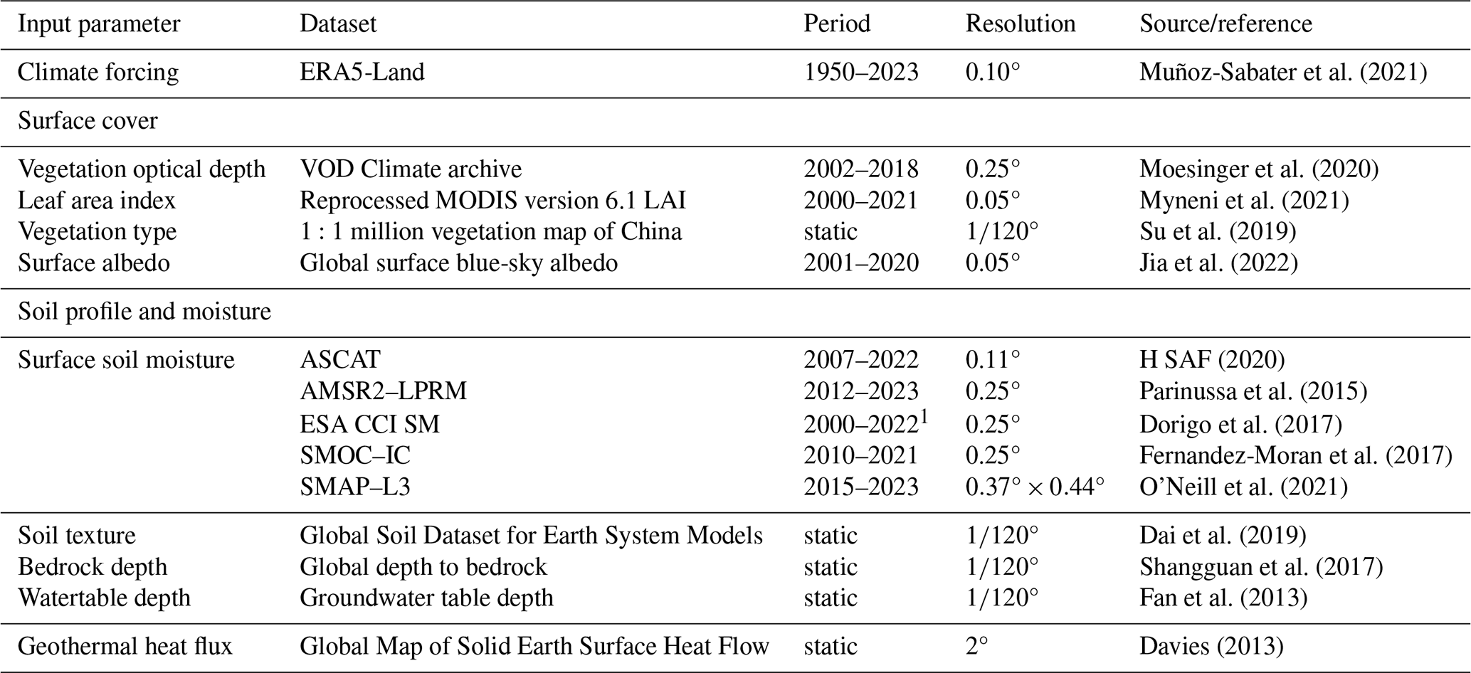
¹ To be consistent with the other soil moisture products, only the period of 2000–2022 are used here, although ESA CCI provides a longer period.

The Q_si and Q_li are either from observations or from a reanalysis dataset (Table 2). The Q_le is computed under the assumption that ground (snow) emits as a gray body:

$$\begin{array}{}\text{(3)}& {\displaystyle }{\displaystyle }{Q}_{\text{le}}=-{\mathit{\epsilon }}_{\mathrm{s}}\mathit{\sigma }{T_{\text{s0}}}^{\mathrm{4}}\end{array}$$

where ε_s (–) is the surface emissivity, and σ is the Stefan–Boltzmann constant of $\mathrm{5.67}\times {\mathrm{10}}^{-\mathrm{8}}$ $\mathrm{W}{\mathrm{m}}^{-\mathrm{2}}{\mathrm{K}}^{-\mathrm{4}}$. The ε_s was set to 0.92 for soil surface, and 0.98 for snow surface (Fleagle and Businger, 1980).

The turbulent exchange of sensible heat Q_h is given by Price and Dunne (1976):

$$\begin{array}{}\text{(4)}& {\displaystyle }& {\displaystyle }{Q}_{\mathrm{h}}={\mathit{\rho }}_{\mathrm{a}}{c}_p{D}_{\mathrm{h}}(T_{\mathrm{a}}-T_{\text{s0}})\text{(5)}& {\displaystyle }& {\displaystyle }{\mathit{\rho }}_{\mathrm{a}}\approx {\displaystyle \frac{P}{R_d{T}_{\mathrm{a}}}}\end{array}$$

where ρ_a is the air density (kg m⁻³), c_p=1004 $\mathrm{J}{\mathrm{kg}}^{-\mathrm{1}}{\mathrm{K}}^{-\mathrm{1}}$ is the specific heat of air, P (Pa) is atmospheric pressure, T_a (K) is near-surface air temperature, and R_d=0.287 $\mathrm{kJ}{\mathrm{kg}}^{-\mathrm{1}}{\mathrm{K}}^{-\mathrm{1}}$ is specific gas constant. The exchange coefficients for heat D_h (–) can be estimated as:

$$\begin{array}{}\text{(6)}& {\displaystyle }{\displaystyle }{D}_{\mathrm{h}}={\displaystyle \frac{{\mathit{\kappa }}^{\mathrm{2}}{u}_z}{{\left(\ln \left(z/z_{\mathrm{0}}\right)\right)}^{\mathrm{2}}}}\end{array}$$

where κ=0.4 is the Von Karman's constant, u_z (m) is the wind speed at the instrument height z (m), and z₀ (m) is the roughness length as 0.015 m for soil surface and 0.001 m for snow surface following Ling and Zhang (2004).

The latent heat flux was calculated via the Priestley–Taylor method (Priestley and Taylor, 1972).

$$\begin{array}{}\text{(7)}& {\displaystyle }{\displaystyle }{Q}_{\mathrm{e}}=S\cdot {\mathit{\alpha }}_{\text{pt}}{\displaystyle \frac{\mathrm{\Delta }(Q_{\mathrm{n}}-Q_{\mathrm{c}})}{\mathrm{\Delta }+\mathit{\gamma }}}\end{array}$$

where S (–) is the evaporation stress factor, α_pt (–) is the Priestley–Taylor coefficient, Q_n (W m⁻²) is the net radiation, Δ (Pa K⁻¹) is the slope of the saturation vapor pressure-temperature curve, and γ (Pa K⁻¹) is psychrometric constant. Δ is determined following Dingman (2015):

$$\begin{array}{}\text{(8)}& {\displaystyle }{\displaystyle }\mathrm{\Delta }={\displaystyle \frac{\mathrm{4098}{e}_{\mathrm{s}}}{(T_{\mathrm{a}}-T_{\text{frz}}+\mathrm{237.3}{)}^{\mathrm{2}}}}\end{array}$$

where T_frz=273.15 K is the freezing point temperature, and e_s (Pa) is saturation vapor pressure derived following Dingman (2015):

$$\begin{array}{}\text{(9)}& {\displaystyle }{\displaystyle }{e}_{\mathrm{s}}=\mathrm{611}\exp \left({\displaystyle \frac{\mathrm{17.3}\left(T_{\mathrm{a}}-T_{\text{frz}}\right)}{T_{\mathrm{a}}-T_{\text{frz}}+\mathrm{237.3}}}\right)\end{array}$$

the γ is calculated using the formula proposed by Brunt (2011):

$$\begin{array}{}\text{(10)}& {\displaystyle }{\displaystyle }\mathit{\gamma }={\displaystyle \frac{c_{p}P}{\mathit{\epsilon }{L}_{\mathrm{v}}}}\end{array}$$

where $L_{\mathrm{v}}=\mathrm{2.471}\times {\mathrm{10}}^{\mathrm{6}}$ J kg⁻¹ is the latent heat of vaporization, and ε is a constant of 0.622 (Dingman, 2015). For each grid, the latent heat flux is treated separately for the bare ground surface, vegetation, and snow. The detailed parameterizations are in Appendix E. In current FPM, Monin–Obukhov similarity theory (for Q_h) and Priestley–Taylor method (for Q_e) were combined to improve simulation efficiency as some previous studies (Agam et al., 2010; Song et al., 2016). We acknowledge that using two different theories may introduce additional uncertainties.

Heat conduction through the snow layer or/and ground surface (Q_c) was given as Liston and Hall (1995):

$$\begin{array}{}\text{(11)}& {\displaystyle }{\displaystyle }{Q}_{\mathrm{c}}=\left\{\begin{array}{ll}(T_{\text{s0}}-T_{\mathrm{s}}){\left(\frac{z_{\mathrm{s}}}{k_{\mathrm{s}}}\right)}^{-\mathrm{1}},& \text{snow-free}\\ (T_{\text{s0}}-T_{\mathrm{s}}){\left(\frac{z_{\text{sn}}}{k_{\text{sn}}}\right)}^{-\mathrm{1}},& \text{snd}\ge \mathrm{0.1}\\ (T_{\text{s0}}-T_{\mathrm{s}}){\left(\frac{z_{\text{sn}}}{k_{\text{sn}}}+\frac{z_s}{k_{\mathrm{s}}}\right)}^{-\mathrm{1}},& \begin{array}{l}\mathrm{0}<\text{snd}<\mathrm{0.1}\\ z_s+z_{\text{sn}}=\mathrm{0.1}\end{array}\end{array}\right.\end{array}$$

where T_s (K) is the temperature at 0.1 m depth, and is either from snow (if snd≥0.1 m) or from soil. The k_s and k_sn ($\mathrm{W}{\mathrm{m}}^{-\mathrm{1}}{\mathrm{K}}^{-\mathrm{1}}$) are the thermal conductivity of the soil and snow at the depth of z_s and z_sn, respectively.

The surface energy balance and heat conduction constitute a coupled non-linear equation system, and was solved iteratively for the surface temperature T_s0, using the Newton–Raphson method.

2.2 Snow scheme

The significant influences of snow cover on soil thermal regime have been well documented (Zhang, 2005). Over the TP, snow cover is minor, with a mean annual snow depth of about 0.002 m (and about 0.01 m in winter) according to the ground observations from the China Meteorological Administration network (Orsolini et al., 2019; Cao et al., 2019b). Consequently, the snow effects are relatively minor in this region. The required degree of model complexity depending on the intended applications. For this reason, a simple snow scheme was incorporated into the initial version of FPM to represent the influences of seasonal snow on soil thermal regime. We acknowledge that the application of the FPM is not recommended in regions with prevalent snow due to its limited capability in simulating snow processes. The snow layer was discretized into multiple layers with a vertical resolution of 0.01 m snow depth (snd) for heat transfer simulations. The snow densification algorithm from Verseghy (1991) was introduced here.

$$\begin{array}{}\text{(12)}& {\displaystyle }{\displaystyle }{\mathit{\rho }}_{\text{sn}}^{t+\mathrm{\Delta }t}=({\mathit{\rho }}_{\text{sn}}^t-{\mathit{\rho }}_{\text{sn}}^{\text{max}})\cdot \exp \left(-\mathrm{0.24}\mathrm{\Delta }t\right)+{\mathit{\rho }}_{\text{sn}}^{\text{max}}\end{array}$$

where ${\mathit{\rho }}_{\text{sn}}^{\text{max}}=\mathrm{300}$ kg m⁻³ is the maximum snow density, and Δt is the simulation time step in day. The fresh snow density was set as 100 kg m⁻³.

The snow albedo is treated separately for non-melting and melting conditions following Douville et al. (1995). For non-melting conditions, a linear decrease is assumed for α_sn, while an exponential decrease is assumed for melting snow due to the presence of liquid water.

$$\begin{array}{}\text{(13)}& {\displaystyle }{\displaystyle }{\mathit{\alpha }}_{\text{sn}}^{t+\mathrm{\Delta }t}=\left\{\begin{array}{ll}{\mathit{\alpha }}_{\text{sn}}^t-\mathrm{0.008}\mathrm{\Delta }t,& \text{non-melting}\\ {\mathit{\alpha }}_{\text{sn}}^{\text{min}}+\left({\mathit{\alpha }}_{\text{sn}}^t-{\mathit{\alpha }}_{\text{sn}}^{\text{min}}\right){\mathrm{e}}^{-\mathrm{0.24}\mathrm{\Delta }t},& \text{melting }\\ {\mathit{\alpha }}_{\text{sn}}^{\text{max}},& \mathrm{\Delta }\text{snd}\ge \mathrm{0.01}\mathrm{m}\end{array}\right.\end{array}$$

where ${\mathit{\alpha }}_{\text{sn}}^{\text{max}}=\mathrm{0.85}$ denotes the maximum snow albedo or the fresh snow albedo, while ${\mathit{\alpha }}_{\text{sn}}^{\text{min}}=\mathrm{0.50}$ is the minimum snow albedo for old snow, and Δsnd (m) refers to the change in snow depth per time step. If there is a significant snowfall, i.e. Δsnd≥0.01 m, snow albedo was reset to the maximum by assuming the snow surface is completely overlaid by the fresh snow.

The snow cover fraction was given as

$$\begin{array}{}\text{(14)}& {\displaystyle }{\displaystyle }\text{SCF}=min\left({\displaystyle \frac{\text{snd}}{{\text{snd}}_{\text{cr}}}},\mathrm{1}\right)\end{array}$$

where snd_cr=0.1 m is the minimum snow depth that ensures complete coverage of the grid cell.

The snow volumetric heat capacity (CV_sn, $\mathrm{J}{\mathrm{m}}^{-\mathrm{3}}{\mathrm{K}}^{-\mathrm{1}}$) and thermal conductivity are treated as functions of snow density (ρ_sn, kg m⁻³) following Douville et al. (1995):

$$\begin{array}{}\text{(15)}& {\displaystyle }& {\displaystyle }{\text{CV}}_{\text{sn}}={\text{CV}}_{\mathrm{i}}{\displaystyle \frac{{\mathit{\rho }}_{\text{sn}}}{{\mathit{\rho }}_{\mathrm{i}}}}\text{(16)}& {\displaystyle }& {\displaystyle }{k}_{\text{sn}}=k_{\mathrm{i}}{\left({\displaystyle \frac{{\mathit{\rho }}_{\text{sn}}}{{\mathit{\rho }}_{\mathrm{w}}}}\right)}^{\mathrm{1.88}}\end{array}$$

where ${\text{CV}}_{\mathrm{i}}=\mathrm{1.93}\times {\mathrm{10}}^{\mathrm{6}}$ $\mathrm{J}{\mathrm{m}}^{-\mathrm{3}}{\mathrm{K}}^{-\mathrm{1}}$ is volumetric heat capacity for ice, k_i=2.22 $\mathrm{W}{\mathrm{m}}^{-\mathrm{1}}{\mathrm{K}}^{-\mathrm{1}}$ is the thermal conductivity of ice, ρ_i=920 kg m⁻³ is ice density, and ρ_w=1000 kg m⁻³ is water density. Snow ablation was heavily simplified by directly using the snow water equivalent from reanalysis. Snowfall temperature equals the near-surface air temperature, capped at 273.15 K. During snowmelt, any simulated snow temperature exceeding 273.15 K is reset to this threshold.

2.3 Ground heat conduction and phase change

The ground temperature T (K) changes over time (t) and depth (z, m), and is numerically solved by the heat conduction for energy transfer and phase change determined by Fourier's law:

$$\begin{array}{}\text{(17)}& {\displaystyle }{\displaystyle }C{\displaystyle \frac{\partial T}{\partial t}}={\displaystyle \frac{\partial }{\partial z}}\left(k{\displaystyle \frac{\partial T}{\partial z}}\right)\end{array}$$

The latent heat during phase change is taken into account through an apparent volumetric heat capacity:

$$\begin{array}{}\text{(18)}& {\displaystyle }{\displaystyle }C={\text{CV}}_{\mathrm{s}}+L_f{\mathit{\rho }}_{\mathrm{w}}{\displaystyle \frac{\partial {\mathit{\theta }}_{\mathrm{u}}}{\partial T}}\end{array}$$

where C and CV_s are the apparent volumetric heat capacity and volumetric heat capacity of soil ($\mathrm{J}{\mathrm{m}}^{-\mathrm{3}}{\mathrm{K}}^{-\mathrm{1}}$), respectively, $L_f=\mathrm{0.334}\times {\mathrm{10}}^{\mathrm{6}}$ J kg⁻¹ is mass specific latent heat of water, θ_u (m³ m⁻³) is the volumetric unfrozen water content or super-cooled water, and T is from the previous step. The unfrozen water was parameterized following Niu and Yang (2006):

$$\begin{array}{}\text{(19)}& {\displaystyle }{\displaystyle }{\mathit{\theta }}_{\mathrm{u}}={\mathit{\theta }}_{\text{sat}}{\left[{\displaystyle \frac{{\mathrm{10}}^{\mathrm{3}}{L}_f\left(T-T_{\text{frz}}\right)}{gT{\mathit{\psi }}_{\text{sat}}}}\right]}^{-\frac{\mathrm{1}}{b}}\end{array}$$

where g=9.80665 m s⁻² is the acceleration due to gravity. The θ_sat (m³ m⁻³), ψ_sat (mm), and b is the saturated soil moisture, saturated matric potential, and Clapp–Hornberger parameter, respectively. They are all derived based on the soil material properties (Appendix A). FPM implements the nonlinear heat-transfer equations in Cartesian coordinates.

Thermal properties of the soil are assumed to be a weighted combination of different components of the soil column. The CV_s is calculated from the volumetric fractions of the constituents as follows Westermann et al. (2016):

$$\begin{array}{}\text{(20)}& {\displaystyle }{\displaystyle }{\text{CV}}_{\mathrm{s}}=\sum _n{f}_n{\text{CV}}_n\end{array}$$

where subscripts n=m, o, w, i, a, and g refer to soil constituents of mineral, organic, water, ice, air, and gravel. In this context, f_n (m³ m⁻³) and C_n ($\mathrm{J}{\mathrm{m}}^{-\mathrm{3}}{\mathrm{K}}^{-\mathrm{1}}$) represent the volumetric content and volumetric heat capacity for each component (Table B1, Appendix B). Similarly, the thermal conductivity of the soil k_s ($\mathrm{W}{\mathrm{m}}^{-\mathrm{1}}{\mathrm{K}}^{-\mathrm{1}}$) is calculated following Cosenza et al. (2003):

$$\begin{array}{}\text{(21)}& {\displaystyle }{\displaystyle }{k}_{\mathrm{s}}={\left(\sum _n{f}_n\sqrt{k_n}\right)}^{\mathrm{2}}\end{array}$$

where k_n is the thermal conductivity ($\mathrm{W}{\mathrm{m}}^{-\mathrm{1}}{\mathrm{K}}^{-\mathrm{1}}$) for each soil component.

For temporal discretization, the model employs a first-order backward Euler scheme with a daily time step. We selected this unconditionally stable implicit method to overcome the strict step-size limitations typically associated with explicit schemes. By preventing numerical divergence even with a relatively coarse temporal resolution, this approach allows for a computationally economical implementation that maintains sufficient fidelity for capturing long-term thermal dynamics. The spatial derivatives are discretized using the control volume method, yielding a tridiagonal system of algebraic equations at each time step that is efficiently solved via the Thomas algorithm.

3 Model setting up and ensemble simulation

3.1 Soil profile

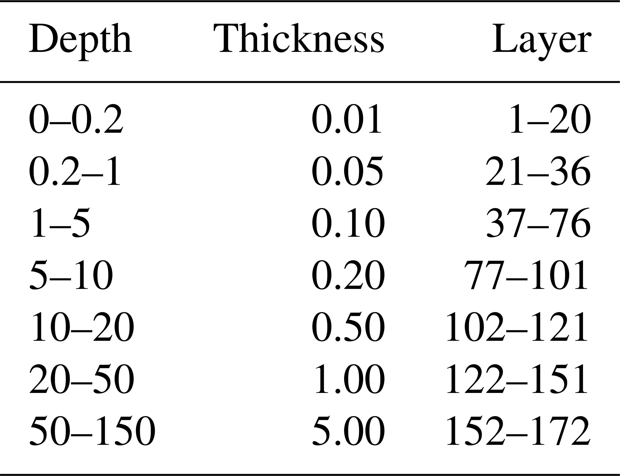
To maintain numerical stability and reduce computational cost, the soil vertical grid size increased from 0.01 m for subsurface to 5.0 m for deep soil (Table E1), similar to the other models (Zheng et al., 2020). The soil column with a total depth of 150 m is discretized to 172 layers. We use the soil texture of the Global Soil Dataset for Earth System Models (GSDE) as it additionally provides the soil gravel content, which is prevalent over the TP (Dai et al., 2019). GSDE has 8 soil layers with a total depth of 3.8 m. The information of the last layer was extended to deeper soil, but was refined based on the bedrock depth from Shangguan et al. (2017). Note that, we assume soil organic matter is absent for soil below 3 m as is normally done in Earth system models (e.g. Chadburn et al., 2015).

3.2 Soil water content

Soil moisture can significantly affect the dynamics of the soil thermal regime through evapotranspiration and by altering soil thermal properties (Göckede et al., 2017; Zwieback et al., 2019). However, in the permafrost regions of the TP, soil moisture exhibits marked heterogeneity and is difficult to accurately represent in models. This challenge stems from uncertainties in soil datasets and climate forcing, as well as the inherent complexities of the rugged terrain. For the current version, the static soil moisture is used. To specify the vertical water distribution within the soil column, we used sub-grid parameterizations from SURFEX and CryoGridLite (Decharme et al., 2006; Masson et al., 2013; Langer et al., 2024). Here, we distinguished four hydrological layers in the subsurface, from the uppermost surface to deep layer, including the: (1) root zone; (2) vadose layer, extending from the root layer downward to the lower boundary or saturated table/bedrock (if present); (3) saturated layer, which lies between the depth of groundwater table and bedrock; and (4) bedrock layer, extends down to the lower boundary. Note that the presence and depth of the saturated layer is estimated based on the groundwater table information from Fan et al. (2013). The root depth is set between 0.05 m for bare soil and 0.5 m for high vegetation, and the typical depth for different vegetation cover is from GEOtop (Endrizzi et al., 2014).

In the root layer, the water content θ_R (m³ m⁻³) is estimated as the ensemble mean of five remote sensing-based products (Table 2, details see Sect. 3.3). The water content for the vadose layer θ_v (m³ m⁻³) is determined based on field capacity θ_fc (m³ m⁻³) and soil porosity ϕ (m³ m⁻³), and an ensemble range is used (see Sect.3.3). Please see Appendix A for the parameterizations of soil properties. In the saturated layer, the water content (θ_sat) is equal to ϕ. The water content of 0.05 m³ m⁻³ was used for the bedrock (Gubler et al., 2013).

3.3 Ensemble simulations for soil hydrology

Although the use of static soil moisture models is common practice for investigating long-term permafrost changes among permafrost researchers (e.g. Jafarov et al., 2012; Qin et al., 2017a; Langer et al., 2024), and four vertical water distribution schemes were implemented in FPM, this estimate is subject to large uncertainty. To allow the propagation of this uncertainty into model results, we introduced both wet and dry variants of the default parameters (see Sect. 3.3). The ensemble simulations – allowing degrees of parameter uncertainties – are widely used for Earth system studies as they generally outperform individual simulations (Cao et al., 2019a; Langer et al., 2024). In this study, the ensemble simulation is produced using reasonable ranges of parameters (Table 3). Both the ensemble range of soil moisture in root layer and vadose zone are assumed here to allow possible uncertainties. The θ_R is derived as an ensemble mean of five state-of-the-art products (Table 2), and the ensemble was produced by $+/-$ (wet/dry soil) standard deviation of all these products. The baseline of θ_v was determined as the mean of θ_fc and θ_sat in previous studies (e.g. Langer et al., 2024). We followed this algorithm, but introduced a dry and wet variants of the θ_v parameter used (Table 3). We emphasize that the ensemble was chosen after considerable tests and comparisons but ultimately remains a subjective choice at this time. The range of the above selected parameters are used for the 45-member ensemble simulation to represent a wide range of permafrost conditions. This approach prevents the simulation from capturing seasonal and long term evolution linked to changes in the soil water content which can be an important driver of permafrost dynamics.

Table 3 Soil moisture (m³ m⁻³) parameters selected for ensemble simulations. The dry and wet variants indicate the parameter ensemble range, and default indicates the standard choice used in model simulation.

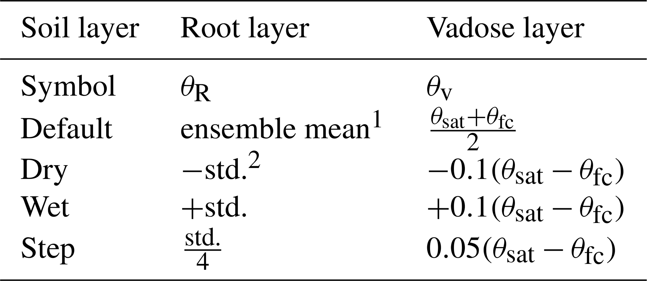
The footnote of ¹ and ² mean the ensemble mean and standard deviation (std.) of five remote-sensing-based soil moisture in Table 2.

3.4 Model settings

The simulation was conducted at a time step of 1 d. A lower boundary condition of geothermal heat flux from Davies (2013) is used (Table 2). To ensure the convergence of soil temperature profile, the model was initialized through a 1000 year spin-up process. This was achieved by cyclically applying the climate forcing data from the first decade (July 1950 to June 1960) one hundred times. Simulation performance was measured by the mean bias (BIAS) as well as root mean square error (RMSE), and more details can be found in Appendix C.

3.5 Diagnosis and analyses of permafrost characteristics

Permafrost is diagnosed following its definition, i.e. the daily soil temperature of a simulation pixel remains at or below 0 °C for two or more years at any simulated depth. Instead of directly using presence/absence of permafrost for individual ensemble member, the permafrost zonation index (PZI), as a fraction (0–1) corresponds to the 45 simulation members identified the probability of permafrost presence for each grid, is introduced to represent permafrost extent here. In such, the PZI can be used to quantitatively explore permafrost changes for each grid. More details of permafrost probability estimate could be found from Obu et al. (2019) and Burke et al. (2020). In this study, we especially focus on the thermal state of permafrost at a depth of 3 m as the near-surface permafrost treated in most land surface models (Burke et al., 2020), and 15 m as the permafrost mean annual ground temperature (MAGT). The permafrost extent for above 100 m is additionally used as reference. The glaciers and lakes from ERA5-Land are masked before permafrost extent analyses. The ALT is estimated from linear interpolation of daily soil temperature. In this study, the period of 2010–2023 is used as the current condition for permafrost.

4 Data

4.1 Climate forcing

FPM is driven by climate forcing from reanalysis, including: near-surface air temperature, wind speed, incoming shortwave radiation, incoming longwave radiation, atmospheric pressure, and snow water equivalent. In this study, the historical climate is taken from the ERA5-Land datasets, produced by the European Centre for Medium-Range Weather Forecasts (ECMWF, Table 2). ERA5-Land is an enhanced land component of ERA5 with a spatial resolution of 0.1° and a coverage from 1950 to the present (Muñoz-Sabater et al., 2021). The reanalyses were evaluated against the in situ observations (Appendix D). Note that the snowfall from ERA5-Land was reported to be over biased due to the significant drawback of precipitation represented in models (Orsolini et al., 2019). For this reason, the simulated snow influences on soil thermal regime were very likely artificially amplified.

4.2 Surface cover

FPM considers the influences of vegetation on permafrost via the latent heat and soil moisture etc. (Appendix E). In FPM, static vegetation is assumed and the vegetation optical depth (VOD), leaf area index (LAI), and vegetation type are required (Table 2). For snow-free periods, the ground albedo is from Jia et al. (2022).

The remote-sensing datasets vary in their temporal coverage, so we used the climatology to represent the long-term conditions. For the VOD and snow-free ground albedo, the daily measurements over the entire recording period were aggregated into a day-of-year climatology using the median, so as to reduce sensitivity to extreme values. The monthly LAI from Myneni et al. (2021) was aggregated to monthly medians. Daily θ_R values were first aggregated into monthly averages for each dataset. These monthly values from the thawing season (June to August) were then used to compute the annual mean. For each soil moisture dataset, the average over the entire recording period was derived, and an ensemble mean across the five datasets was calculated and employed as model inputs. Note that only the measurements from the thawing season were used to derive VOD.

4.3 Datasets used for model evaluation

4.3.1 Synthesis datasets

In this study, 10 synthesis sites with both meteorological and soil temperature measurements were used to conduct the detailed evaluations (Table 4, Fig. 1). The soil information, i.e. soil texture and moisture are also available at the sites. Note that the missing atmospheric observations are filled with downscaled reanalyses following the algorithm presented by Fiddes and Gruber (2014), Cao et al. (2017a).

Zhao et al. (2021)Cao et al. (2018)

Table 4 Metadata for the synthesis sites with both permafrost and atmospheric forcing measurements, including latitude (Lat, ° N), longitude (Lon, ° E), elevation (Ele, m), vegetation type, mean annual air temperature (MAAT, °C), mean soil moisture (SM, m³ m⁻³) in growth season, mean annual ground temperature (MAGT, °C), active layer thickness (ALT, m), and measurement period.

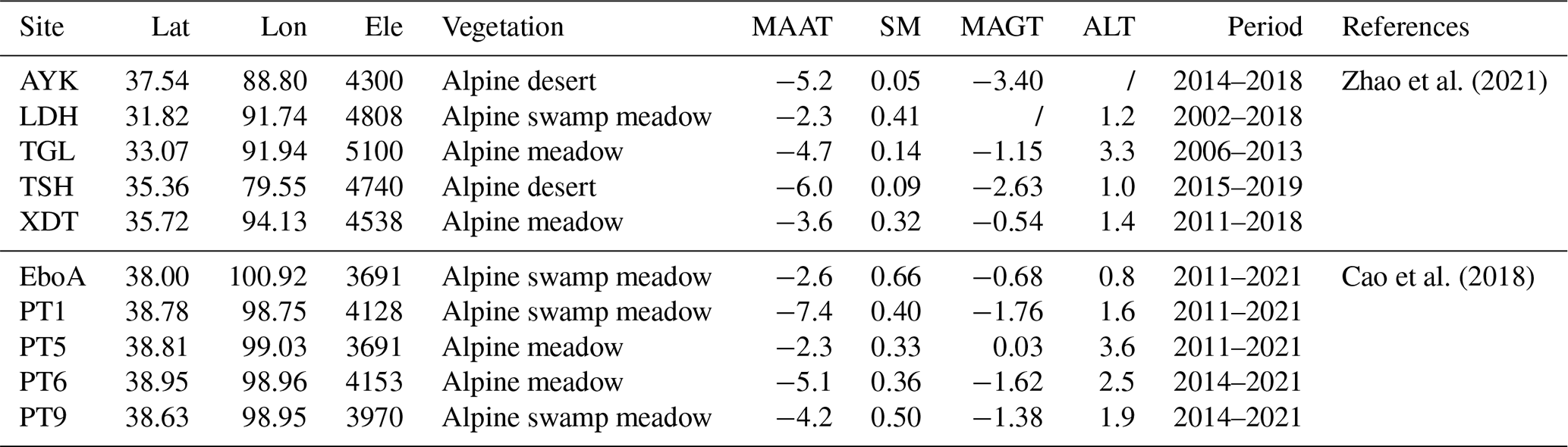
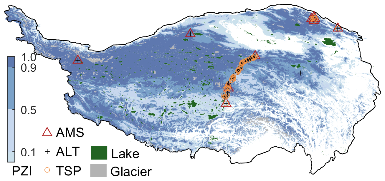
Figure 1 In situ observations used for model evaluation, including comprehensive observation sites with both the active layer soil temperature and atmospheric observations from the automatic meteorological system (AMS), active layer thickness (ALT) from soil temperature profile, and the permafrost thermal state (TSP) from boreholes. The permafrost zonation index (PZI) is from Cao et al. (2019b).

4.3.2 Active layer thickness and borehole temperature measurements

Active layer thickness and borehole temperature measurements from the Global Terrestrial Network for Permafrost (GTN-P, Biskaborn et al., 2019) and literature (see Supplement for details) are used here to evaluate model performance. This yielded 247 ALT measurements from 128 sites (Fig. 1). The measured mean ALT was about 2.3±0.8 m with a range of 0.7–4.9 m. ALTs are derived from different land covers, including Alpine desert, alpine steppe, alpine meadow, and alpine swamp meadow, indicating that the evaluation presented here is representative.

The MAGT measurements between the depths of 7.5 and 40 m are treated as the thermal state of permafrost, and this leads to 71 boreholes with 364 MAGT measurements that were used for model evaluation. The measured mean MAGT was about $-\mathrm{0.95}\pm \mathrm{1.1}$ °C with a range from −4.2 to 2.2 °C. Among the measurements, 19 borehole sites with a long times-series (≥1 decade) were further used to evaluate the modeled TSP changes.

4.3.3 Referenced permafrost maps and process-based simulations

We use five permafrost maps as reference datasets to evaluate the modeled permafrost area. These are (1) the new map of permafrost distribution on the TP via the temperature at the top of permafrost (TTOP) model (Zou et al., 2017); (2) the permafrost zonation index map compiled based on the statistical relationship between topoclimatic predictors (e.g. air temperature, snow, and vegetation) and permafrost zonation (Cao et al., 2019b); (3) the global permafrost zonation index with the normal and cold variant (Gruber, 2012); (4) the Northern Hemisphere permafrost map derived via the TTOP model (Obu et al., 2019), and (5) the outputs from LSM of Noah (Wu et al., 2018).

Process-based permafrost simulations across the TP remain relatively scarce, and the direct evaluation of such simulations against observations is currently unavailable. Consequently, this study utilizes permafrost conditions and dynamics derived from the Noah (Wu et al., 2018), CLM (Guo and Wang, 2013), GIPL2 (Qin et al., 2017a), and GBEHM (Zheng et al., 2020) models as a basis for comparing the permafrost thermal regime. The referenced permafrost extent and thermal regime is estimated for different time periods, using different modeling paradigms and forcing, and are not perfect or a “source of truth”. We treat them as the “best available” reference.

5 Results

5.1 Model evaluations

Our evaluation results showed the overall RMSE of daily soil temperature in the active layer was 1.8 °C with a BIAS of 0.4 °C (Fig. 2). FPM showed relatively worse performance in areas with alpine swamp meadow (RMSE=2.7 °C), with warm bias in summer and cold bias in winter. This is attributed to poorly prescribed soil information, i.e. peat layer and soil moisture. At the sites with alpine desert, the overestimated soil moisture (by about 25 %) at 0.5 m depth leads to a colder simulated soil temperature in summer (Fig. 2a). To demonstrate the hypothesis, we conducted the additional simulations using observed atmospheric forcing and soil profile from borehole measurements. The simulated soil temperature was significantly improved by 1.9 °C, indicating the simulations could be improved with more reliable climate forcing and soil profile (Fig. 2).

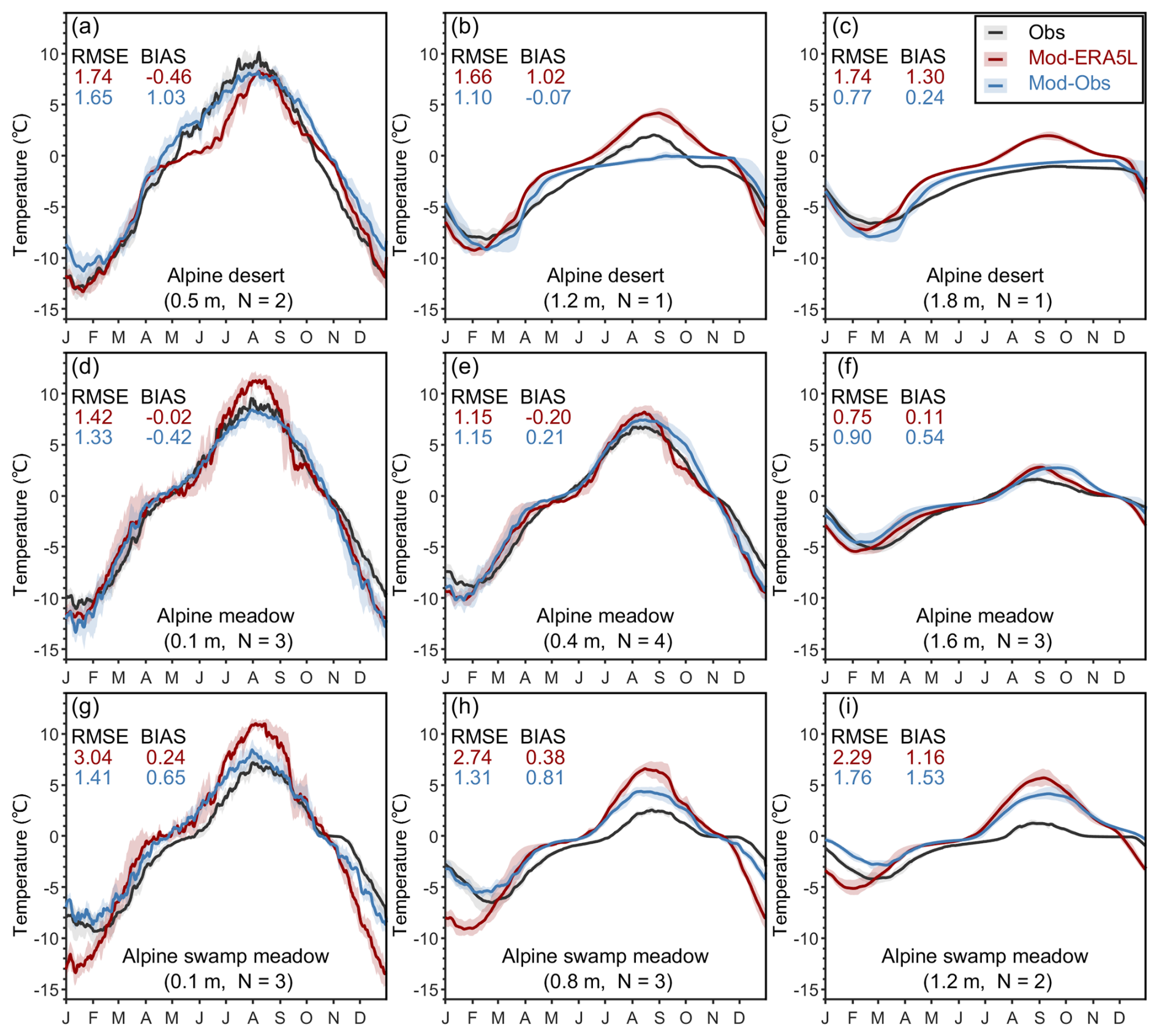
Figure 2 Comparison of simulated and observed day-of-year soil temperature in the active layer across the synthesis sites. The daily soil temperature present is averaged for each vegetation type and soil depth based on all available sites and years. The soil depth and numbers of sites (N) are given in parentheses. The sites used for each vegetation type and depth differ based on data availability. Observations are in black (Obs), red lines show the simulation forced by reanalyses (MOD-ERA5L), and the blue lines represent that forced by observed atmospheric forcing and in situ soil information (if available, MOD-Obs). The shaded areas depict the ensemble range from the 25th to 75th. The ensemble of observation forced simulation are produced using results from different sites and additional ranges of soil moisture (see Table 3).

FPM generally has good agreement with observed ALTs with the overall RMSE of 1.0 m, and slightly underestimated ALT ($\text{BIAS}=-\mathrm{0.1}$ m) due to the cold-biased summer air temperature (Figs. 3 and D1). Following the relatively worse soil temperature, ALT was over-biased in areas with alpine swamp meadow. The additional simulation with observed forcing and soil information, again, showed more promising results (RMSE=0.7 m). The ALT bias was within ±1 m at most (64 %) evaluated cells (Fig. 3).

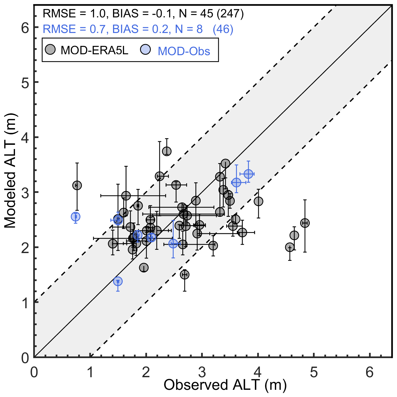
Figure 3 Evaluation of modeled active layer thickness (ALT). The ensemble mean from FPM simulations (MOD-ERA5L) are given in black dot, with the whiskers representing the range between the 25th and 75th percentiles. The observed mean was aggregated from multiple measurements at a single site or from multiple sites within the same grid. N indicates the number of grids used for evaluation after aggregating sites within the same grid, and the number of measurements was given in parentheses. The additional simulation driven by observed meteorological forcing (MOD-Obs) are given in blue. Dashed lines indicate ±1 m.

FPM is found to underestimate the MAGT with an overall mean BIAS of −0.3 °C, which is aligned with the cold-biased air temperature (Fig. D1a). The overall MAGT RMSE was 1.0 °C (Fig. 4), and about 65(93) % sites have a bias within ±1(2) °C. Although the MAGT change trend is well addressed by FPM with an RMSE of 0.22 °C per decade, it is found even greater than the observed mean MAGT trend of 0.12±0.09 °C per decade (Fig. 5). This indicates that the simulated MAGT trend may not be reliable. In fact, the permafrost warming at the measured sites was relatively gentle (with a range from −0.07 to 0.3 °C per decade) compared to that in high latitudes (Intergovernmental Panel On Climate Change, 2022). This is because the permafrost temperature over the TP is very “warm”, and the heat from atmosphere was consumed by phase change rather than temperature increase (also see Fig. 7). The significant latent heat introduce additional challenge for reproducing MAGT trend.

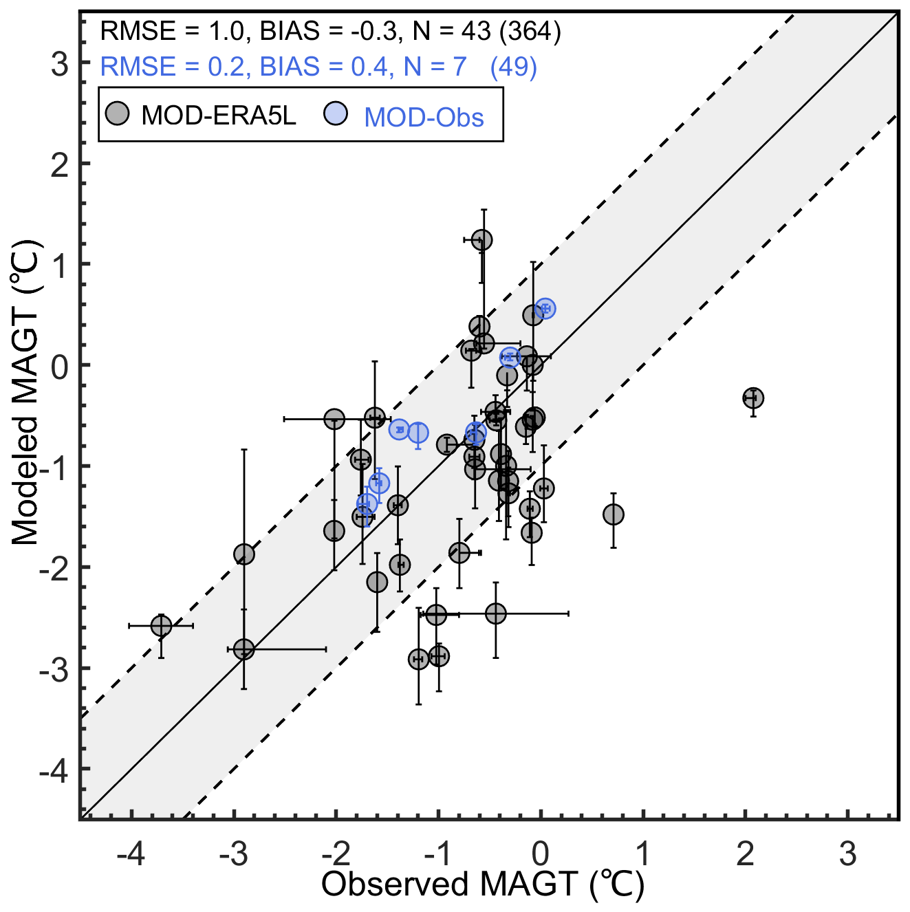
Figure 4 Same as Fig. 3, but for the mean annual ground temperature (MAGT) at 15 m depth. Dashed lines indicate ±1 °C.

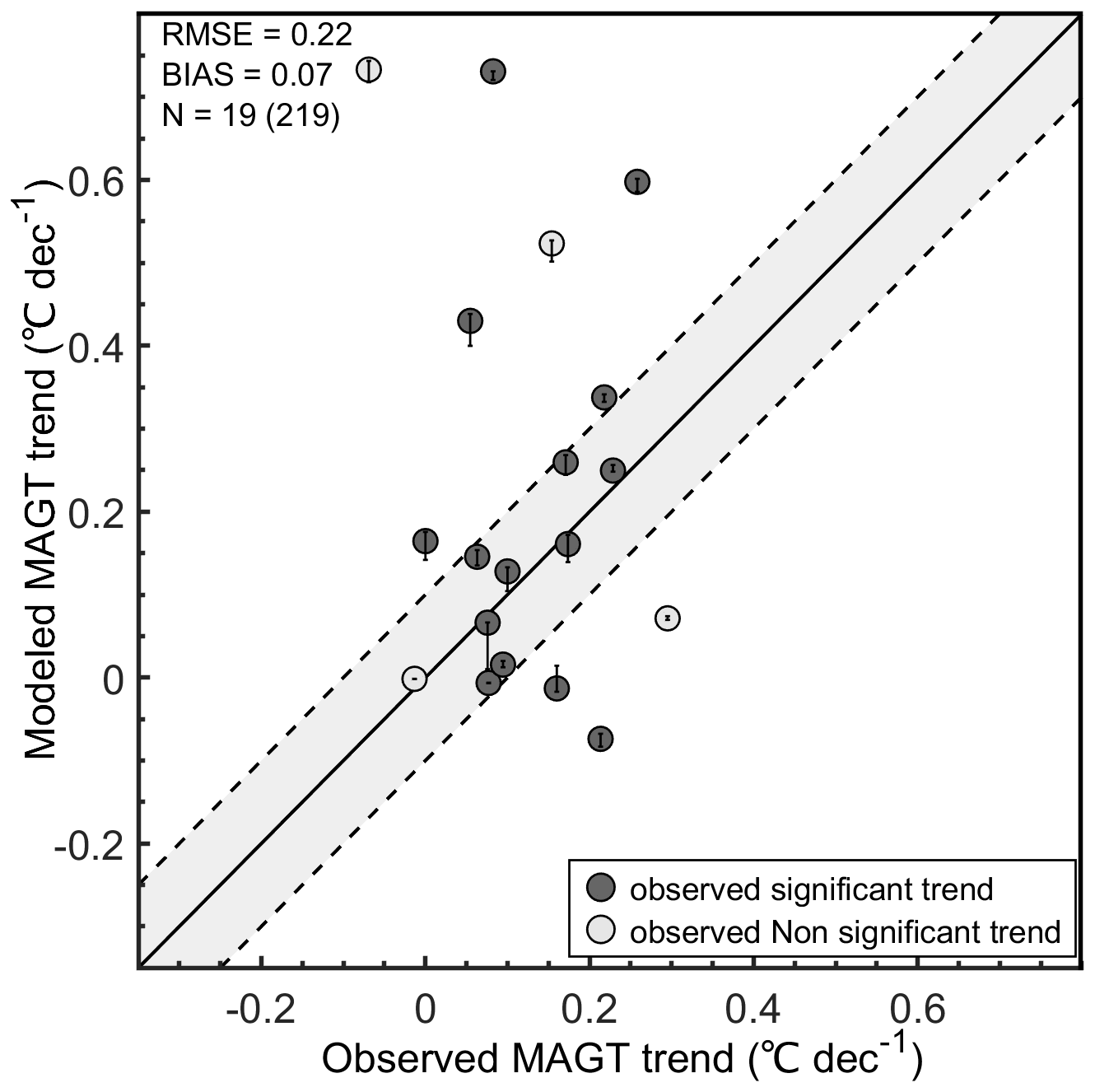
Figure 5 Same as Fig. 3, but for the changes of mean annual ground temperature (MAGT) at 15 m depth. Only the sites with long-term observations (≥1 decade) are used here. The filled dots are sites with observed significant trends. Dashed lines indicate ±0.1 °C per decade.

Excluding glaciers and lakes, the estimated current (2010–2023) permafrost area was about $\mathrm{1.07}\pm \mathrm{0.02}\times {\mathrm{10}}^{\mathrm{6}}$  km² (Fig. 8) based on the ensemble simulations from FPM. This is found reasonable compared to the referenced ensemble mean of $\mathrm{1.15}\pm \mathrm{0.12}\times {\mathrm{10}}^{\mathrm{6}}$  km² (Fig. 9).

5.2 Changes in active layer thickness

The ensemble simulations from FPM showed the current (2010–2023) overall mean ALT was about 2.68±0.82 m over the TP. The results are found align with the previous simulations, for example, 2.1–2.4 m (1981–2013) from GIPL2 (Qin et al., 2017a) and 2.01 m (1981–2000) from CLM (Guo and Wang, 2013). Our results indicated that about 33.0 % of permafrost regions have an ALT greater than 3 m, highlighting that the widely used land surface models and reanalyses with shallow soil column may not be sufficient for permafrost studies over the TP.

The long-term simulation showed that ALT had a inter-annual trends with a decreasing trend between 1950–1980 (−0.14 m per decade), followed by a continuous increasing trend (0.13 m per decade). Consequently, the ALT over TP increased by 0.41 m since 1980 (Fig. 6b). While the simulated ALT increase rate was similar to that of Guo and Wang (2013), it was lower than those reported by Zheng et al. (2020), Qin et al. (2017a), both of which indicated a rate of ∼0.3 m per decade. Notably, long-term observations showed that the ALT increased at a rate of 0.19 m per decade, suggesting that our results are likely underestimates (Zhao et al., 2020).

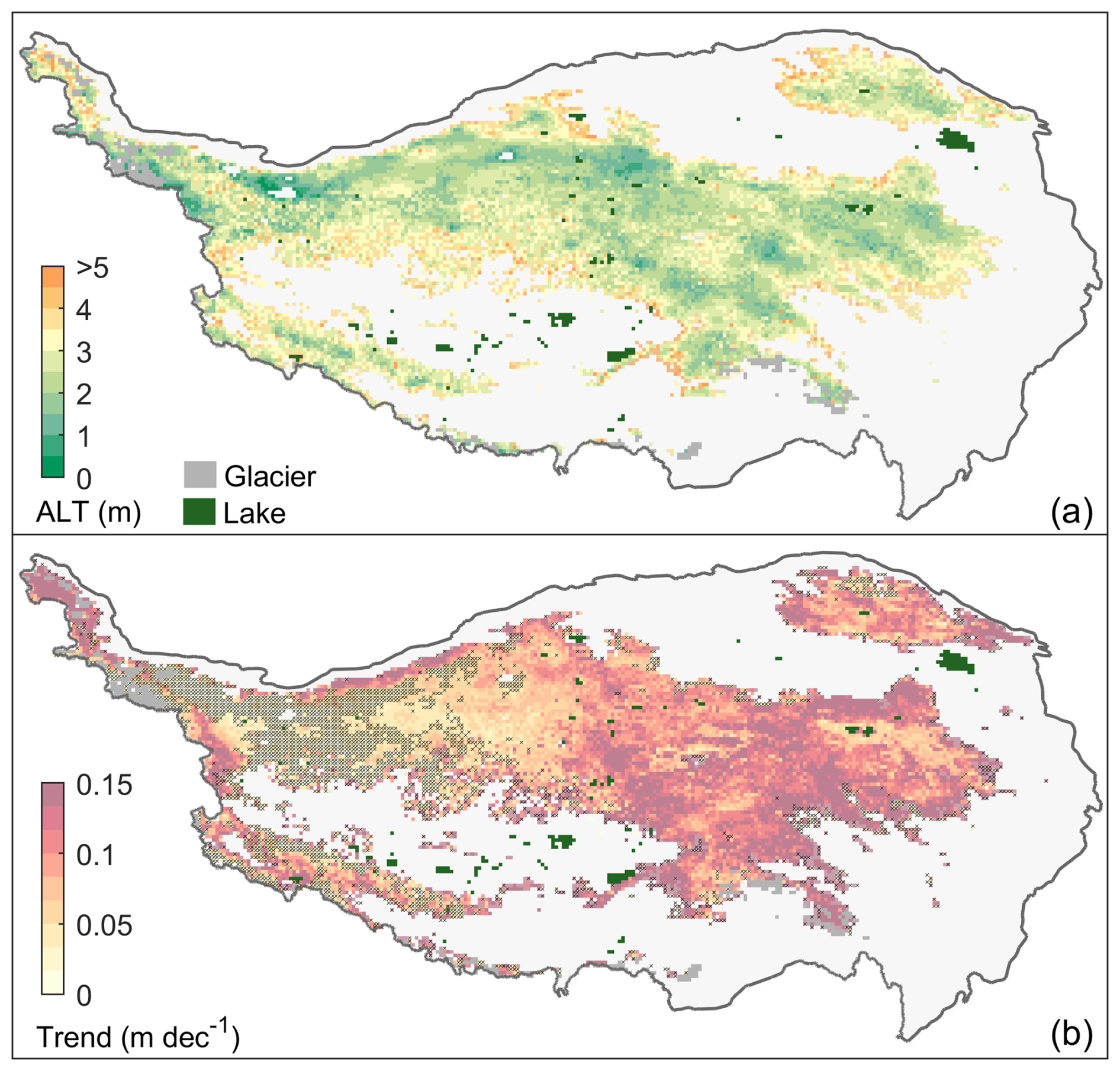
Figure 6 (a) The modeled current (2010–2023) mean active layer thickness (ALT), and (b) its change rate from 1980 to 2023. The areas without significant trends are marked by ×. Glaciers and lakes are from ERA5-Land.

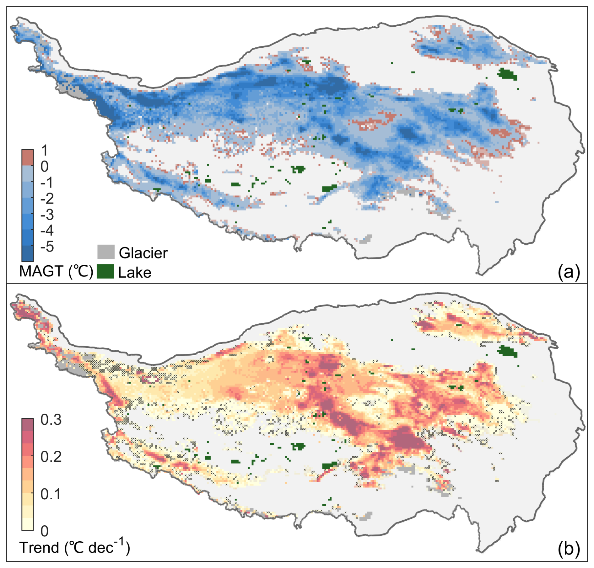
Figure 7 (a) The modeled current (2010–2023) mean annual ground temperatures at the depth of 15 m, and (b) its change rate from 1980 to 2023. The areas without significant trends are marked by ×.

5.3 Changes in permafrost temperature

The mean annual ground temperature at the depth of 15 m (MAGT₁₅) is used to represent the thermal state of permafrost. The modeled overall mean MAGT₁₅ (2010–2023) was about $-\mathrm{1.8}\pm \mathrm{2.0}$ °C for the permafrost regions over the TP and shows a wide range from −19.2 to 3.4 °C (Fig. 7a). The permafrost thermal regime is found similar to the outputs from Noah LSM, i.e. −1.6 °C (Wu et al., 2018). Our simulations revealed that the overall MAGT₁₅ increased by approximately 0.22 °C since 1950, with a more dramatic warming of 0.11 °C per decade since 1980. Similar to the ALT, MAGT shows a clear cooling trend (−0.02 °C per decade) between 1950–1980 corresponding to the changes in near surface air temperature.

The permafrost warming trend was found to be MAGT-dependent, with a slower rate for warmer permafrost. For example, the permafrost warming rate was about 0.05±0.06 °C per decade for areas with MAGT₁₅ between −1–0 °C, and 0.17±0.09 °C per decade for permafrost regions colder than −2 °C. This is consistent with observations (Biskaborn et al., 2019; Zhao et al., 2020), as heat is consumed as latent heat during the ice phase change for permafrost that is close to thawing.

5.4 Changes in permafrost extent

The permafrost area decreased by approximately 9.5×10⁴ km² during 1950–2023, but increased by 4.3 % from 1950 to 1980 following cooling of the near-surface air temperature (Fig. 9a). Permafrost area decreased at a rate of 3.3×10⁴ km² per decade, or a total area of 12.4 %, since 1980. Our results showed that the model with shallow soil column would significantly underestimate permafrost area but overestimated permafrost degradation. Take the top 3 m as an example, which has been widely used in the land surface model. The estimated near-surface (top 3 m) permafrost area (7.9×10⁴ km²) was about 26.0 % smaller compared to the ground “truth”, or 31.4 % smaller than the simulations with sufficient soil column (e.g. 100 m, Fig. 9b). Furthermore, by omitting permafrost below a depth of 3 m, the shallow soil model incorrectly classified areas with deep permafrost as permafrost-free. Therefore, the permafrost degradation rate was overestimated by about 42 % (3.3×10⁴ vs. 4.7×10⁴ km² per decade) (Fig. 9). This highlights that the current land surface models with shallow soil column can lead to significant uncertainties in permafrost simulations.

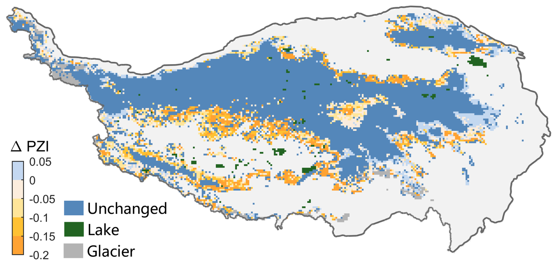
Figure 8 Changes of permafrost extent, as permafrost zonation index (PZI), between 2010–2023 and 1981–1990. The PZI is 45-member ensemble probability of permafrost where permafrost is defined by the daily temperature at 15 m depth, and negative values indicate a loss in permafrost extent.

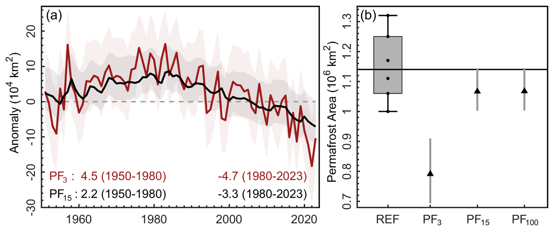
Figure 9 (a) Anomaly of permafrost area since 1950, and (b) comparison of estimated current (2010–2023) permafrost area from FPM simulations with referenced estimations (Sect. 4.3.3). The subscript means the depth above which permafrost is diagnosed. The permafrost area trend (10⁴ km² per decade) is estimated for the periods before and after 1980, separately, and curves are 25th and 75th.

5.5 Simulation spread

The ensemble simulation revealed that the variation in soil moisture translated into considerable influences on simulated permafrost characteristics (Fig. 10), with the overall mean standard deviation was about 0.26 m in ALT and about 0.31 °C in MAGT. Notably, the input soil moisture datasets themselves exhibited substantial variability, with mean standard deviation of 0.11 m³ m⁻³ in root zone and 0.14 m³ m⁻³ in vadose zone (Fig. E1). The propagation of input uncertainties into significant permafrost simulation bias thus highlights the essential role of obtaining more reliable soil moisture datasets for advancing our capacity to simulate permafrost changes.

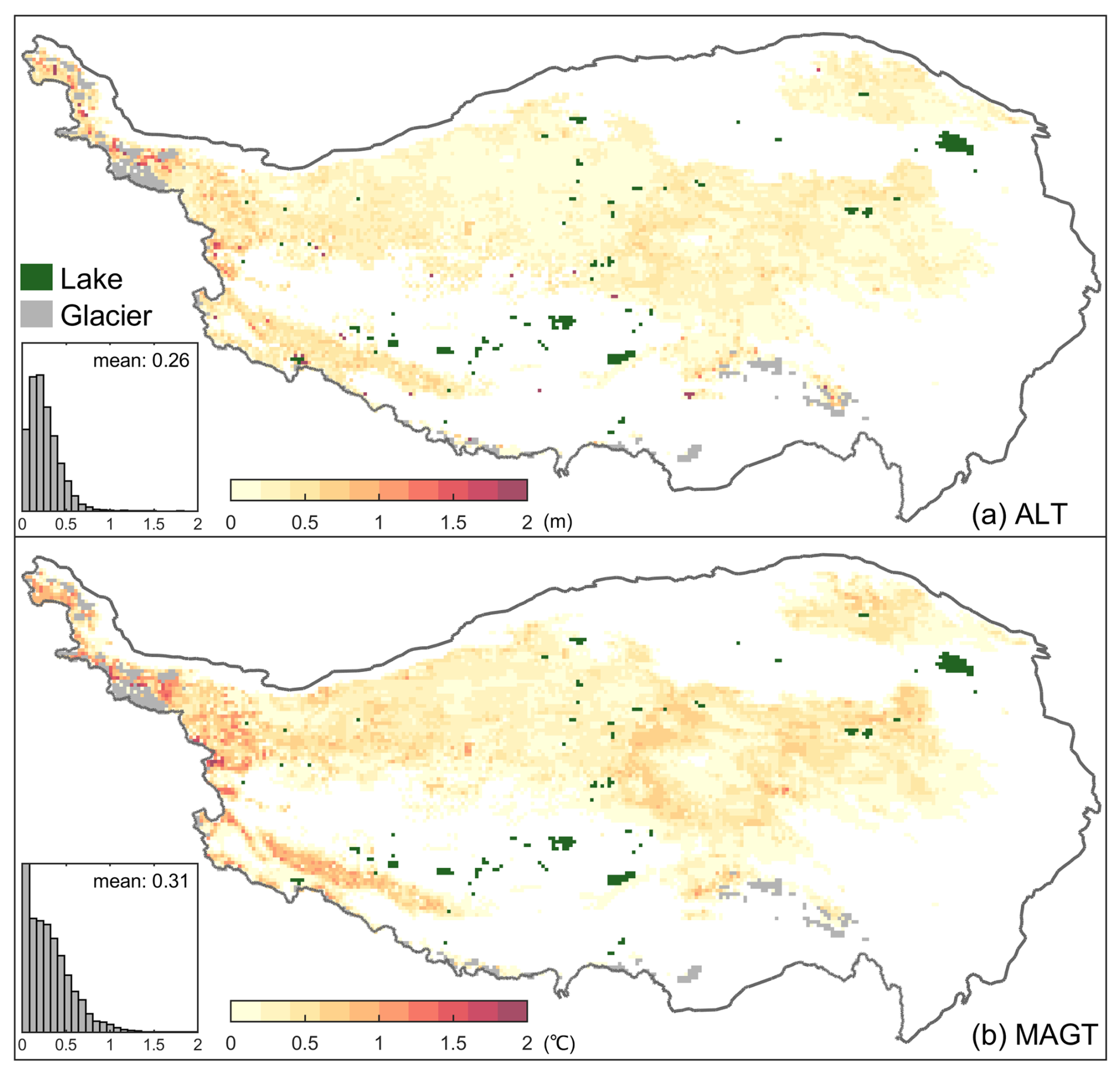
Figure 10 The standard deviation of (a) simulated active layer thickness (ALT) and (b) mean annual ground temperature (MAGT) based on the 45-member ensemble simulations which accounted the possible soil moisture spread in root and vadose zones.

6 Discussions

6.1 Uncertainties from climate forcing and input datasets

We used the ERA5-Land reanalyses as model forcing. However, the ERA5-Land is found cold biased in near-surface air temperature (Appendix D, Fig. D1), leading to underestimated ALT as well as MAGT (Figs. 6 and 7). In fact, permafrost simulations are hampered by reduced reanalyses quality in cold regions primarily due to inherent challenges in representing nonlinear processes involving ice, or its phase change near 0 °C (Cao and Gruber, 2025). The poorly described soil column, especially the soil organic matter, put additional uncertainty for permafrost simulations.

6.2 Model limitations

In this study, we introduced and demonstrated the suitability of FPM for large-scale permafrost simulation. For the initial version of FPM, there are four main limitations. First, the snow scheme is simplistic, although significant influences of snow cover on soil thermal regime have been well documented (Zhang, 2005). FPM currently does not consider the snow mass balance, and, therefore, additionally requires snow water equivalent as input. Further, the snow cover fraction used here was developed for high latitudes and does not consider the influences of complex terrain, which may redistribute the snow cover and lead to strong heterogeneity for the soil thermal regime. While the simple snow scheme seems adequate for the TP with little snow, considerable efforts are required to improve snow processes if FPM would applied to snow-prevalent areas, i.e. the high latitudes.

Second, FPM does not consider the water balance, and the static surface conditions, including vegetation and albedo (varies with season but remains unchanged among years), were assumed via using the remote-sensing-based climatology. This means the influences of surface and sub-surface changes are not accounted for and limited the model ability in predicting long-term permafrost changes.

Third, the fine-scale influences (i.e. debris and peat layer) are either not or simply represented here due to the simulation scale (∼10 km). This may overestimate permafrost degradation, especially for the areas near the permafrost lower limit, where the relict permafrost was found (Fig. 8, Cao et al., 2021).

Fourth, FPM does not consider the thermokarst processes or the so-called “abrupt thaw” raised by excess ice loss. The thermokarst was thought as local-scale tipping element that would remarkably accelerate permafrost degradation (Devoie et al., 2019).

6.3 Comparison with other permafrost models

Our results are found comparable to previous simulations derived from the geothermal numerical models (e.g. Qin et al., 2017a; Chen et al., 2025) as well as land surface models (e.g. Guo and Wang, 2013; Wu et al., 2018; Zheng et al., 2020). FPM, as the stand-alone permafrost model, benefits from the consideration of land-atmosphere processes (i.e. the surface energy balance and vegetation effects) typically not included in geothermal numerical models, while maintaining the deep soil column and suitable numerical solver for soil phase change. In addition, the land-surface-scheme designed structure and streamlined processes (i.e. its efficient simulation of latent heat) make it suitable for large-scale ensemble simulations. Different from the other land surface scheme models with rich processes beyonds permafrost, such as SUTRA (McKenzie et al., 2007), Advanced Terrestrial Simulator (Jan et al., 2020), and CryoGrid 3 (Westermann et al., 2023), which are applied to fine scales, the initial FPM aim to provide a flexible yet simple platform for large-scale permafrost simulation studies.

6.4 Future developments

Previous studies reported that the permafrost processes of the Earth system model in CMIP6 is limited improved compared to the previous generation of CMIP5 (e.g. Burke et al., 2020), and current Earth system models generally have weak ability in representing permafrost (Schädel et al., 2024). This highlights the urgent need to develop the stand-alone permafrost model. Since the required inputs are derived from global datasets, this opens the opportunity for global permafrost simulation with the FPM platform. The incorporation of a state-of-the-art snow scheme – particularly critical for high-latitude permafrost processes – will further enhance this capability. We hope with improved permafrost ground ice maps and a rigorously validated solution (addressing both physical processes and numerical solver aspects), we can implement excess ice loss processes within FPM to represent permafrost “abrupt thaw”. We hope FPM could be further improved via incorporating lateral heat transfer, as described by Sun et al. (2023), making FPM a cross-scale platform for understanding diverse permafrost landscapes.

7 Conclusions

In this study, we introduce a new land surface scheme specifically designed for permafrost applications, the Flexible Permafrost Model (FPM). This model serves as a flexible platform to explore novel parameterizations for a variety of permafrost processes. To demonstrate the utility of FPM for supporting permafrost studies, we apply the model to permafrost studies over the Tibetan Plateau. Our simulation results are compared to in situ observations and published permafrost extent. We summarize the main contributions and insights of this work as the following:

• 1.

  FPM shows suitability in reproducing permafrost characteristics, such as active layer thickness, and the thermal state. With more reliable inputs, especially soil profile, FPM-based simulations can be further improved;

• 2.

  Simulations indicated that the current (2010–2023) mean active layer thickness was about 2.68±0.82 m, permafrost temperature at a depth of 15 m was about $-\mathrm{1.8}\pm \mathrm{2.0}$ °C, and permafrost extent was about $\mathrm{1.07}\pm \mathrm{0.02}\times {\mathrm{10}}^{\mathrm{6}}$  km² over the Tibetan Plateau, and is comparable with previous model outputs;

• 3.

  The process-based historical simulation revealed steady permafrost degradation over the Tibetan Plateau since 1980. The active layer thickness increased by 0.41 m, permafrost temperature at 15 m depth increased at a rate of 0.11±0.01 °C per decade, and permafrost extent degraded by about 12.4 %. Evaluations against observations and comparisons with reference studies indicate that the rate of increase in active layer thickness is likely underestimated;

• 4.

  Our simulations indicate that current land surface models employing shallow soil columns are inadequate for permafrost research on the Tibetan Plateau, since they have generally underestimated permafrost extent while overestimating degradation rates. Such inadequacy may also pose challenges in other regions characterized by deep active layers (i.e. >3 m);

• 5.

  This study highlights the ongoing efforts in stand-alone process-based permafrost model development. We hope that in the future, with more available stand-alone land-scheme-designed permafrost models, the permafrost community will provide a simulation benchmark for the Earth system model developments as well as the climate change assessment at a global scale.

Appendix A: Soil organic matter properties

FPM considers the impacts of organic matter on soil hydraulic properties following CoLM (Dai et al., 2003) and SURFEX (Masson et al., 2013):

$$\begin{array}{}\text{(A1)}& {\displaystyle }& {\displaystyle }\mathit{\tau }=f_{\mathrm{o}}{\mathit{\tau }}^{\mathrm{o}}+f_{\mathrm{m}}{\mathit{\tau }}^{\mathrm{m}}+f_{\mathrm{g}}{\mathit{\tau }}^{\mathrm{g}}\text{(A2)}& {\displaystyle }& {\displaystyle }{f}_{\mathrm{o}}+f_{\mathrm{m}}+f_{\mathrm{g}}=\mathrm{1}\end{array}$$

where f_o (m³ m⁻³), f_m (m³ m⁻³), and f_g (m³ m⁻³) are the fractions of organic matter, mineral and gravel, respectively. The τ refers to the soil hydraulic properties, including: slope of the retention curve b (–), soil matric potential ψ (–), soil porosity ϕ (m³ m⁻³), field capacity θ_fc (m³ m⁻³), and wilting point θ_wp (m³ m⁻³). For gravel, ϕ is set as 0.05 m³ m⁻³, and others are set to 0, assuming the soil hydraulic properties are not directly affected by gravel.

The soil organic matter properties τ^o were implicitly accounted for in the FPM:

$$\begin{array}{}\text{(A3)}& {\displaystyle }& {\displaystyle }{b}^{\mathrm{o}}=min\left(\mathrm{2.7}+\mathrm{9.3}\times {\displaystyle \frac{z_i}{z_{\text{sap}}}},\mathrm{12.0}\right)\text{(A4)}& {\displaystyle }& {\displaystyle }{\mathit{\psi }}_{\text{sat}}^{\mathrm{o}}=min\left(-\mathrm{10.3}+\mathrm{0.2}\times {\displaystyle \frac{z_i}{z_{\text{sap}}}},-\mathrm{10.1}\right)\text{(A5)}& {\displaystyle }& {\displaystyle }{\mathit{\varphi }}^{\mathrm{o}}=max\left(\mathrm{0.93}-\mathrm{0.1}\times {\displaystyle \frac{z_i}{z_{\text{sap}}}},\mathrm{0.83}\right)\text{(A6)}& {\displaystyle }& {\displaystyle }{\mathit{\theta }}_{\text{fc}}^{\mathrm{o}}=min\left(\mathrm{0.37}+\mathrm{0.35}\times {\displaystyle \frac{z_i}{z_{\text{sap}}}},\mathrm{0.72}\right)\text{(A7)}& {\displaystyle }& {\displaystyle }{\mathit{\theta }}_{\text{wp}}^{\mathrm{o}}=min\left(\mathrm{0.07}+\mathrm{0.15}\times {\displaystyle \frac{z_i}{z_{\text{sap}}}},\mathrm{0.22}\right)\end{array}$$

where z_i (m) is the soil depth for soil grid of i, and z_sap=0.5 m is the depth that organic matter takes on the characteristics of sapric peat.

The mineral soil hydraulic properties were approximated as:

$$\begin{array}{}\text{(A8)}& {\displaystyle }& {\displaystyle }{b}^{\mathrm{m}}=\mathrm{2.91}+\mathrm{15.9}{f}_{\text{clay}}\text{(A9)}& {\displaystyle }& {\displaystyle }{\mathit{\psi }}_{\text{sat}}^{\mathrm{m}}=-\mathrm{10}\times {\mathrm{10}}^{\left(\mathrm{1.88}-\mathrm{1.31}{f}_{\text{sand}}\right)}\text{(A10)}& {\displaystyle }& {\displaystyle }{\mathit{\varphi }}^{\mathrm{m}}=\mathrm{0.489}-\mathrm{0.126}{f}_{\text{sand}}\text{(A11)}& {\displaystyle }& {\displaystyle }{\mathit{\theta }}_{\text{fc}}^{\mathrm{m}}=\mathrm{0.45}{\left(f_{\text{clay}}\right)}^{\mathrm{0.3496}}\text{(A12)}& {\displaystyle }& {\displaystyle }{\mathit{\theta }}_{\text{wp}}^{\mathrm{m}}=\mathrm{0.37}\sqrt{f_{\text{clay}}}\end{array}$$

where f_clay (m³ m⁻³) and f_sand (m³ m⁻³) are the volumetric content of clay and sand to the total mineral soil, respectively.

Appendix B: Nomenclature

In this study, Q (W m⁻²) refers to surface energy balance terms, subscripts identify the term (si: incoming shortwave radiation; li: incoming longwave radiation; le: emitted longwave radiation; h: turbulent exchange of sensible heat; e: turbulent exchange of latent heat; c: energy transport due to conduction; n: net radiation; and m: the energy flux available for melt). We use k ($\mathrm{W}{\mathrm{m}}^{-\mathrm{1}}{\mathrm{K}}^{-\mathrm{1}}$), CV ($\mathrm{J}{\mathrm{m}}^{-\mathrm{3}}{\mathrm{K}}^{-\mathrm{1}}$), and ρ (kg m⁻³) to represent thermal conductivity, volumetric heat capacity, and density, respectively. The subscript identifies each source (s: soil; sn: snow; m: mineral; o: organic; w: water; i: ice; a: air; and g: gravel). The volumetric contents for each soil component is represented by f (m³ m⁻³).

Table B1 Nomenclature and input parameters for Flexible Permafrost Model (FPM).

Appendix C: Evaluation metrics

The evaluation metrics of bias (BIAS) and root-mean-square-error (RMSE) were used here to evaluate model performance.

$$\begin{array}{}\text{(C1)}& {\displaystyle }& {\displaystyle }\text{BIAS}={\displaystyle \frac{\mathrm{1}}{N}}\sum _{i=\mathrm{1}}^N(\text{MOD}-\text{OBS}),\text{(C2)}& {\displaystyle }& {\displaystyle }\text{RMSE}=\sqrt{{\displaystyle \frac{\mathrm{1}}{N}}\sum _{i=\mathrm{1}}^N(\text{MOD}-\text{OBS}{)}^{\mathrm{2}}},\end{array}$$

where OBS and MOD represent the variables of interest (i.e. mean annual ground temperature and active layer thickness) from in situ observations and the simulations.

Appendix D: Evaluation of model forcing

The climate forcing was evaluated against in situ daily observations from the synthesis sites (Table 4). Our evaluation results indicate that there is generally a cold bias of the near-surface air temperature (−1.9 °C) for the ERA5-Land, and the RMSE was about 3.5 °C (Fig. D1). While ERA5-Land slightly overestimated the incoming short-wave radiation (bias=10.3 W m⁻²), the incoming long-wave radiation was underestimated by about −24.1 W m⁻². Overall, the evaluation results indicate that the meteorological variables in the reanalysis dataset are generally consistent with the observations and can be used as suitable forcing/inputs for the numerical simulation.

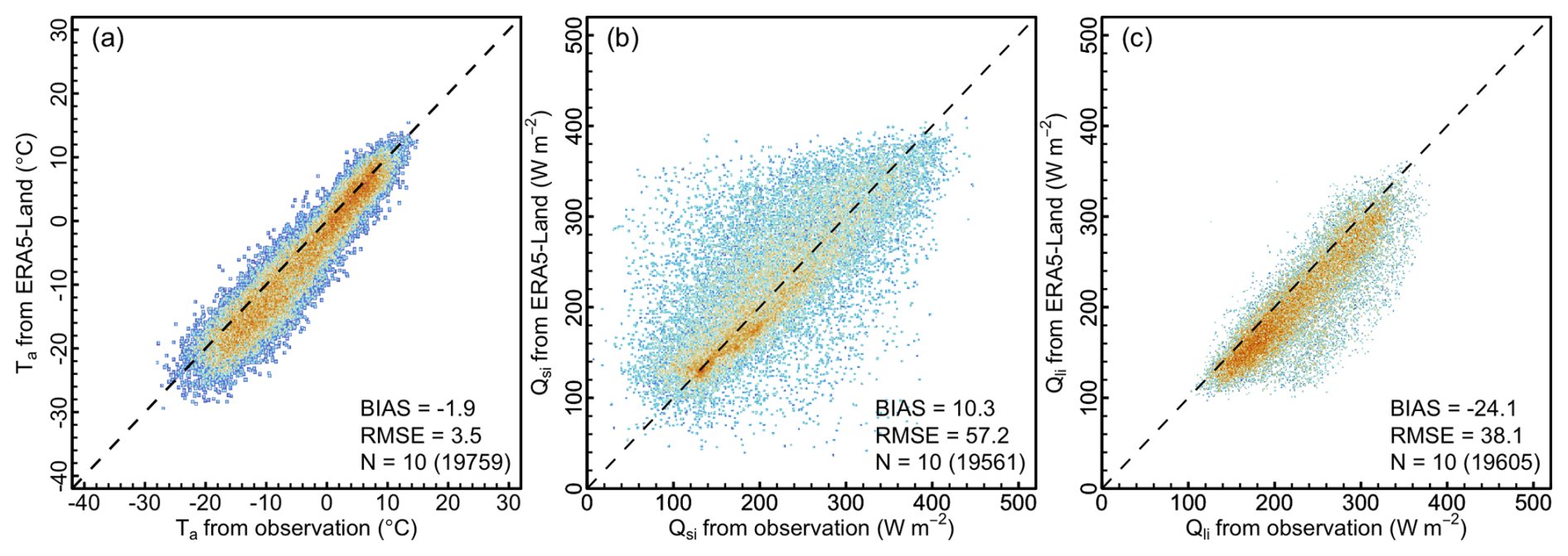
Figure D1 Evaluation of the daily (a) near-surface air temperature (T_a), (b) incoming short-wave radiation (Q_si), and (c) incoming long-wave radiation (Q_li) from ERA5-Land. The number of meteorological stations (measurements) used for the evaluation are given as N.

Appendix E: Latent heat from Priestley–Taylor method

The latent heat flux (Q_e) is treated differently depending on the snow cover, and the FPM uses the Priestley–Taylor method by generally following Martens et al. (2017). If snow is absent, Q_e is the sum of latent heat for bare soil $Q_{\mathrm{e}}^{\mathrm{s}}$ (W m⁻²) and covered vegetation $Q_{\mathrm{e}}^{\mathrm{v}}$ (W m⁻²).

$$\begin{array}{}\text{(E1)}& {\displaystyle }{\displaystyle }{Q}_{\mathrm{e}}=Q_{\mathrm{e}}^{\mathrm{s}}+Q_{\mathrm{e}}^{\mathrm{v}}\end{array}$$

where $Q_{\mathrm{e}}^{\mathrm{s}}$ and $Q_{\mathrm{e}}^{\mathrm{v}}$ are given as

$$\begin{array}{}\text{(E2)}& {\displaystyle }& {\displaystyle }{Q}_{\mathrm{e}}^{\mathrm{s}}=S_{\mathrm{s}}{\mathit{\alpha }}_{\text{pt}}{\displaystyle \frac{\mathrm{\Delta }(Q_{\mathrm{n}}^{\mathrm{s}}-Q_{\mathrm{c}})}{\mathrm{\Delta }+\mathit{\gamma }}}\text{(E3)}& {\displaystyle }& {\displaystyle }{Q}_{\mathrm{e}}^{\mathrm{v}}=S_{\mathrm{v}}{\mathit{\alpha }}_{\text{pt}}{\displaystyle \frac{\mathrm{\Delta }{Q}_{\mathrm{n}}^{\mathrm{v}}}{\mathrm{\Delta }+\mathit{\gamma }}}\end{array}$$

where $Q_{\mathrm{n}}^{\mathrm{s}}$ and $Q_{\mathrm{n}}^{\mathrm{v}}$ are the net radiation partitioned for bare soil and vegetation, and derived following Fisher et al. (2008).

$$\begin{array}{}\text{(E4)}& {\displaystyle }& {\displaystyle }{Q}_{\mathrm{n}}^{\mathrm{s}}=f_{\mathrm{s}}{Q}_{\mathrm{n}}\text{(E5)}& {\displaystyle }& {\displaystyle }{Q}_{\mathrm{n}}^{\mathrm{v}}=(\mathrm{1}-f_{\mathrm{s}})Q_{\mathrm{n}}\end{array}$$

where Q_n (W m⁻²) is the total net radiation, f_s (–) is fractional net radiation reached to the bare soil, and is treated as

$$\begin{array}{}\text{(E6)}& {\displaystyle }{\displaystyle }{f}_{\mathrm{s}}=\exp (-k_{\text{Rn}}LAI)\end{array}$$

where k_Rn = 0.6 is extinction coefficient from Impens and Lemeur (1969), and LAI (–) is Leaf Area Index from MODIS (Table 2).

While α_pt is normally set to 1.26 for snow-free areas following the original study (Priestley and Taylor, 1972), many studies reported that it is site-specific, depending on the surface conditions (e.g. Constantin et al., 2015; Martens et al., 2017). In FPM, the parameterization scheme that solves the influences of vegetation and soil moisture on latent heat was used. This is achieved via introducing the evaporation stress factor S (–). The S for bare soil (S_s) and vegetation (S_v) are defined as:

$$\begin{array}{}\text{(E7)}& {\displaystyle }& {\displaystyle }{S}_{\mathrm{s}}=\mathrm{1}-{\displaystyle \frac{{\mathit{\theta }}_{\mathrm{c}}-{\mathit{\theta }}_{\mathrm{R}}}{{\mathit{\theta }}_{\mathrm{c}}-{\mathit{\theta }}_{\mathrm{r}}}}\text{(E8)}& {\displaystyle }& {\displaystyle }{S}_{\mathrm{v}}=\sqrt{{\displaystyle \frac{\text{VOD}}{{\text{VOD}}_{\text{max}}}}}\left(\mathrm{1}-{\left({\displaystyle \frac{{\mathit{\theta }}_{\mathrm{c}}-{\mathit{\theta }}_{\mathrm{R}}}{{\mathit{\theta }}_{\mathrm{c}}-{\mathit{\theta }}_{\text{wp}}}}\right)}^{\mathrm{2}}\right)\end{array}$$

where θ_c (m³ m⁻³) is the critical soil moisture, θ_R (m³ m⁻³) is the soil moisture in the root zone layer, θ_r (m³ m⁻³) is the residual soil moisture, θ_wp (m³ m⁻³) is soil moisture content of wilting point, VOD (–) is vegetation optical depth, and VOD_max is the maximum VOD for a given simulation cell. The θ_c is variable depending on the soil texture, and we used the parameters from Zhu et al. (2019). The θ_wp is given in Appendix A, and θ_r is constant of 0.05 m³ m⁻³ following Fisher et al. (2008). The VOD is from Moesinger et al. (2020).

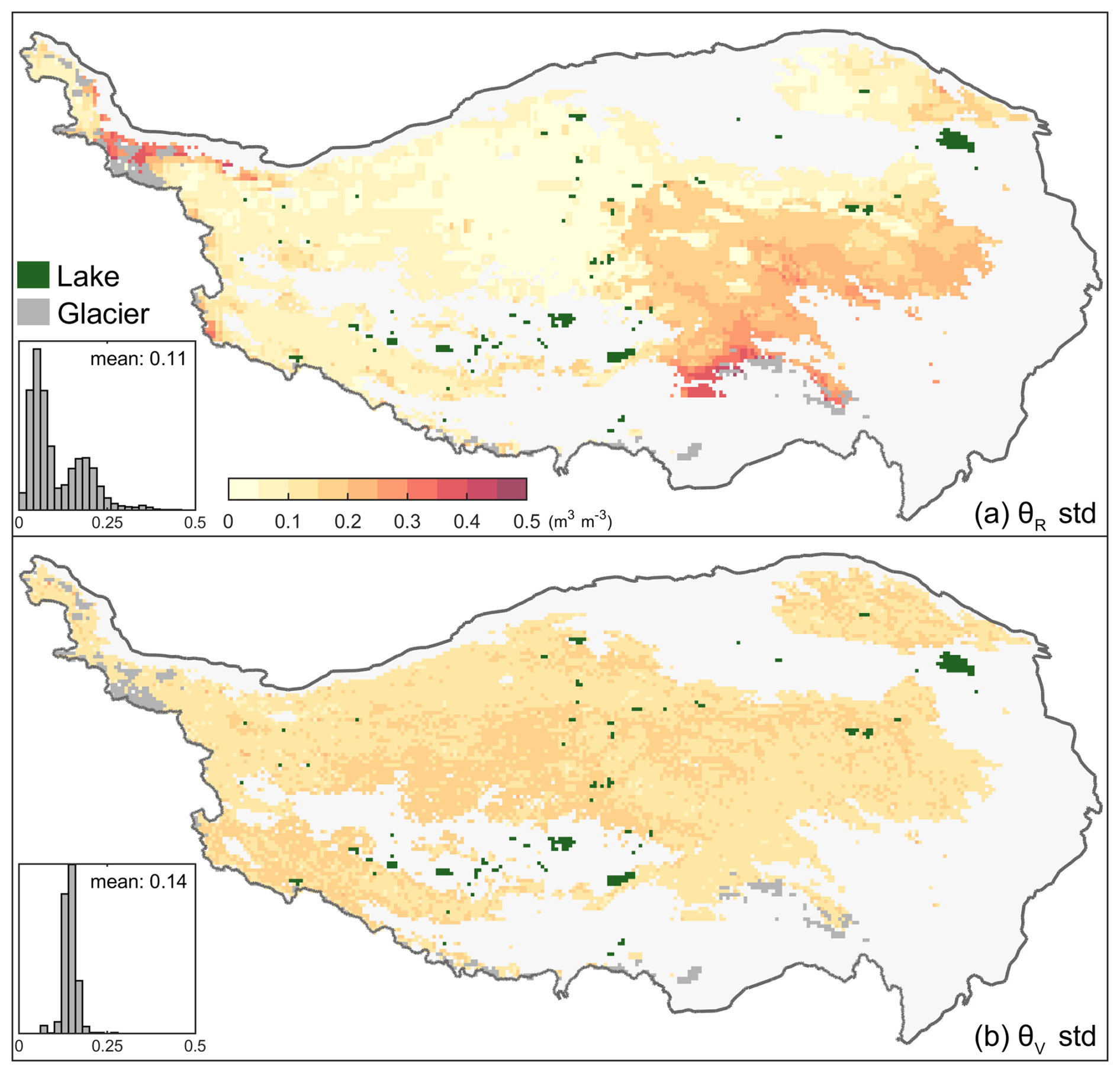
Figure E1 The standard deviation (std.) of the soil moisture spread in (a) root (θ_R) and (b) vadose (θ_v) zones.

Table E1 Ground layer depths (m) and thicknesses (m) for the FPM ground layers configuration.

If snow is present, the Q_e for a given cell is derived as the weighted mean of the snow and soil cover fractions (SCF), assuming no latent heat via vegetation:

$$\begin{array}{}\text{(E9)}& {\displaystyle }{\displaystyle }{Q}_{\mathrm{e}}=\text{SCF}\cdot Q_{\mathrm{e}}^{\text{sn}}+\left(\mathrm{1}-\text{SCF}\right)\cdot Q_{\mathrm{e}}^{\mathrm{s}}\end{array}$$

where $Q_{\mathrm{e}}^{\text{sn}}$ is the latent heat from snow-covered area, and is given as

$$\begin{array}{}\text{(E10)}& {\displaystyle }{\displaystyle }{Q}_{\mathrm{e}}^{\text{sn}}=S_{\text{sn}}{\mathit{\alpha }}_{\text{pt}}{\displaystyle \frac{\mathrm{\Delta }(Q_{\mathrm{n}}^{\text{sn}}-Q_{\mathrm{c}})}{\mathrm{\Delta }+\mathit{\gamma }}}\end{array}$$

where S_sn and α_pt are set to 1 and 0.95, respectively.