A model of water extraction from the subglacial hydrologic system under idealized conditions

Subglacial water modulates glacier velocity across a wide range of space and time scales by influencing friction at the glacier bed. Observations show ice acceleration due to supraglacial lake drainage and water draining through moulins, where both configurations involve water inputs to the bed. Here we consider the reverse: water extraction from the subglacial hydrologic system, which is a proposed intervention method intended to slow the flow of glaciers and reduce the associated sea-level rise. Removing subglacial water results in different dynamics than injecting water, and we hypothesize that understanding these processes will allow for improved characterization of the physics of subglacial hydrology. We set up these model experiments in the Subglacial Hydrology And Kinetic, Transient Interactions (SHAKTI) model coupled with the Ice-sheet and Sea-level System Model (ISSM). By analyzing the problem of an isolated borehole in a background pressure field to determine the region of extraction influence, we find an approximate analytical solution which shows that the water pressure returns to the background value approximately as a logarithm with distance. The benefit of the analytical solution is that the dependence of uncertain parameters is clear and may be used alongside data to constrain subglacial hydrology models. We find good agreement between this analytical result and numerical SHAKTI simulations. Using the coupled SHAKTI-ISSM model, we perform transient model experiments on Helheim Glacier, Greenland and Thwaites Glacier, Antarctica, to determine the effects of water extraction on glacier velocity. With continuous pumping, we simulate a velocity decrease on the order of 1 %, which depends on the site location. The response time to pumping initiation and the recovery time, following cessation, scale according to effective pressure, with typical times on the order of hours to days. These results demonstrate that water extraction is a method of probing the subglacial hydrologic system to better constrain the uncertain physics, and that further research is required to assess its effectiveness as an intervention method.

1 Introduction

Water flowing beneath glaciers influences ice velocity on short (e.g., daily) to longer (e.g., seasonal, annual, decadal) timescales. For mountain glaciers that primarily flow over bedrock, water flow along the ice-bed interface pressurizes cavities and can coalesce into channels (Kamb, 1987; Hewitt, 2011; Flowers, 2015). For ice streams and outlet glaciers, such as the Thwaites Glacier, Antarctica or Helheim Glacier, Greenland, nearly all of their motion comes from slip at the base, where ice flows over water-saturated sediment (Alley et al., 1986; Kamb, 2001; Minchew and Joughin, 2020; Stevens et al., 2022a). In both cases, water at the ice-bed interface can act as a lubricant, allowing glaciers to accelerate. Fast glacier slip also produces water as frictional heating melts the ice, potentially initiating a positive feedback (Schoof and Mantelli, 2021). Effective pressure, defined as the local difference between ice weight and water pressure, is a key control on glacier sliding speed. In steady state, at low effective pressure (high water pressure), additional water leads to glacier acceleration. In higher effective pressure regions (lower water pressure), additional water reduces glacier velocity due to increased efficiency in water flux (Iken and Bindschadler, 1986; Zwally et al., 2002; Schoof, 2010; Hewitt, 2013). On shorter time-scales, glaciers respond to the sudden addition of water from the drainage of supraglacial lakes and streams into moulins. Here water is added at a rate much faster than the subglacial hydrological network adapts, leading to localized acceleration (Das et al., 2008; Andrews et al., 2014; Stevens et al., 2016; Mejía et al., 2021, 2022; Stevens et al., 2022b). Understanding the response of glaciers to meltwater is an ongoing challenge as climate changes and glaciers recede, accelerate, and decay.

In the context of disappearing glaciers and sea-level rise, researchers have proposed ways of conserving glacier ice, i.e., intervention strategies that mitigate ice mass loss due to climate change (Moore et al., 2018), and these ideas have rightly sparked debate (e.g., Moon, 2018; Carey et al., 2022; Flamm and Shibata, 2025; Siegert et al., 2025). One proposed mechanism to slow the speed of glaciers is to extract water from beneath glaciers, in an effort to increase the subglacial effective pressure (i.e., lower the subglacial water pressure), thereby increasing the subglacial friction and reducing glacier velocity (e.g., Lockley et al., 2020). Although this idea could have merit at glaciers where the velocity response to added meltwater is acceleration, it would likely not work in locations with efficient drainage. Siegert et al. (2025) describe a host of issues with subglacial pumping as an intervention strategy and indicate that further research is required before further consideration. To this aim, the focus of this paper is to understand the impact of water exaction on subglacial hydrology in a model.

A natural analog for intervention in subglacial hydrology is the seasonal addition of meltwater. Observations of glacier velocity in Greenland show seasonal variation, driven by surface melt reaching the subglacial hydrologic system (Moon et al., 2014; Vijay et al., 2019; Solgaard et al., 2022). The meltwater driven seasonal patterns have frequently been categorized into two responses, although not all glaciers fit neatly into these two categories. For some glaciers, the velocity increases with meltwater, with the highest velocities observed in summer. In this case, additional meltwater decreases friction, and allows for faster glacier sliding. For other glaciers, meltwater input reduces the glacier velocity, indicating that adding water to these subglacial environments increases the friction by presumably developing a channelized network that efficiently drains the bed. In terms of subglacial water pressure, adding meltwater increases water pressure for glaciers that accelerate over the course of the melt season, and decreases water pressure for glaciers that decelerate. As a glacier intervention strategy, extracting water from a glacier that accelerates with meltwater should theoretically reduce its velocity, but may have the opposite effect on a glacier that would decelerate. Although a glacier may respond as in aggregate, the subglacial hydrologic system below glaciers is heterogeneous and the physical processes that control whether a glacier will respond to water extraction are largely unknown.

With only sparse direct observations of subglacial water pressure, subglacial hydrology models offer a way to understand controls on effective pressure and sliding (Flowers, 2015; de Fleurian et al., 2018). The Glacier Drainage System (GlaDS) model has been applied to numerous glacier systems to simulate the evolution of water pressure (e.g., Werder et al., 2013; Poinar et al., 2019; Dow et al., 2022; Ehrenfeucht et al., 2025). The Subglacial Hydrology and Kinetic, Transient Interactions (SHAKTI) model is a continuum model that has also been applied to numerous glaciers to determine the subglacial conduit geometry and local effective pressure (e.g., Sommers et al., 2018, 2023; Narayanan et al., 2025). By coupling SHAKTI to ice velocity in the Ice-sheet and Sea-level System Model, Sommers et al. (2024) simulated Helheim Glacier to determine the realm of influence of terminus effects on velocity patterns as compared to regions dominated by hydrology. Here we use the SHAKTI model, but focus on advances that could be generalized to all subglacial hydrology models.

Pumping water into and out of groundwater aquifers is a technique for characterizing permeability, among other properties. As water is extracted (injected), the height of the aquifer is lowered (raised), indicating a decrease (increase) in hydraulic head, i.e., the ratio of water pressure to specific gravity, $h=p_{\mathrm{w}}/\left({\mathit{\rho }}_{\mathrm{w}}g\right)$. In the case of extraction, the flow results in a reduction of hydraulic head that spreads outward in time in a way that can be calculated analytically, i.e., the Theis solution (Fitts, 2002). Using time-varying borehole pressure data alongside the analytical solution allows researchers to determine unknown parameters, such as the permeability. If there is recharge in the system, i.e., water flow into the region during pumping, the solution approaches a steady balance between recharge and extraction, which can also be calculated analytically. The Theis method was used to characterize a deep subglacial groundwater system in Greenland (Liljedahl et al., 2021) where they found stratigraphic layers with differing permeability. Similarly, by characterizing the response of a subglacial hydrologic system to water extraction, it may be possible to obtain new constraints on the conductivity and melt production of the subglacial environment from borehole pressure data. A key distinction between the subglacial environment and a groundwater aquifer is that while the hydraulic conductivity of the porous media in a groundwater system remains constant, the hydraulic conductivity of the subglacial drainage system changes as the subglacial gap height opens and closes due to melt and creep closure.

Although we are not aware of any studies probing the subglacial hydrologic system via water extraction, measuring the response to water input has been tried, such as in the field experiments by Engelhardt and Kamb (1997, 1998). In a series of drilling campaigns on the Siple Coast, Antarctica, these researchers used hot water to drill holes to the bed of numerous glaciers. They measured the water pressure as the hot-water drilling fluid connected to the subglacial system and equilibrated. Then they used the pressure pulse to determine the effective permeability of the subglacial system. Characterizing the permeability as an effective water layer thickness, they found that it was on the order of 2 mm. Engelhardt et al. (1990) found water pressure to be near or slightly above the overburden ice pressure. These findings are consistent with work by Alley (1996), Weertman and Birchfield (1982), and Doyle et al. (2022).

In this paper, we analyze the effects of extracting water on the subglacial environment through mathematical analysis and computational modeling. In the following sections, we start by analyzing the results of a simulation pumping at a single location on Helheim Glacier in southeast Greenland, as motivation. We develop analytical and numerical solutions, showing the radius of influence of water extraction, the local effective pressure, and the response time to pumping. Next, we return to coupled SHAKTI-ISSM numerical simulations at Helheim, with multiple extraction sites. We then examine water extraction at Thwaites Glacier, Antarctica. Following these results, we provide context for our models in terms of subglacial hydrology and glacier intervention as well as discuss next steps and comment on avenues for further research.

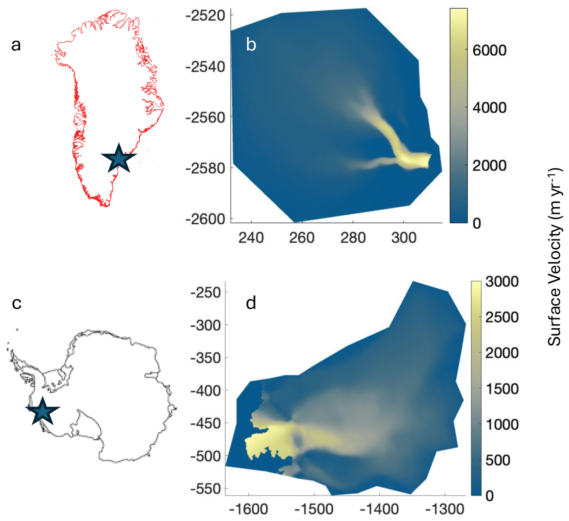
Figure 1 Simulation context: (a) Location of Helheim Glacier in southeast Greenland. (b) Modeled ice velocity on model domain. (c) location of Thwaites Glacier in West Antarctica. (d) Modeled ice velocity on the model domain. All x and y coordinates throughout the figures are given in Polar Stereographic projections with units of km.

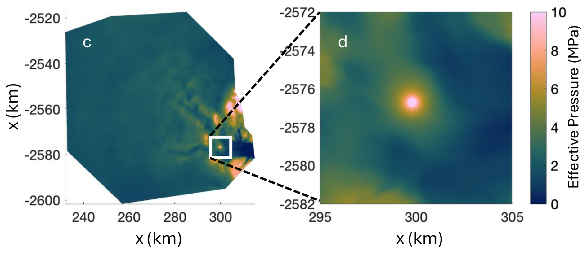
Figure 2 Single extraction site at Helheim Glacier, Greenland: Pumping test simulation at a single extraction site near the confluence of the two main branches, with a pumping rate of 1 m³ s⁻¹, shows high effective pressure around the pumping site.

2 Approach

Here we describe the setting and rationale for our numerical simulations. We consider two glacier systems. The first glacier is Helheim Glacier, a large, marine-terminating outlet glacier in southeast Greenland (Sermersooq, Kalaallit Nunaat; homeland of the Tunumiit, the Greenlandic Inuit of East Greenland). The location of Helheim and the simulation domain are shown in Fig. 1a, b. Helheim is among the largest contributors to sea-level rise from glaciers in Greenland (Mankoff et al., 2020), moving several km per year in its main trunk. The second glacier is Thwaites Glacier in West Antarctica (Fig. 1c, d). Thwaites is a fast-moving outlet glacier that is accelerating, retreating, and losing mass. Thwaites currently contributes meaningfully to sea-level rise. If Thwaites were to collapse, it could trigger a collapse of the wider West Antarctic Ice Sheet, which would lead to significant sea-level rise (Scambos et al., 2017).

To simulate the ice dynamics and subglacial hydrology below these glaciers, we use the Subglacial Hydrology And Kinetic, Transient Interactions (SHAKTI) model built into the Ice-sheet and Sea-level System Model (ISSM). SHAKTI-ISSM simulations have previously been conducted on Helheim Glacier (Sommers et al., 2023, 2024), yielding an established model environment for testing water extraction. Here we use the shallow-shelf approximation (SSA; Morland, 1987; MacAyeal, 1989; Morlighem et al., 2013; Sommers et al., 2024) as the stress balance solver built into ISSM to describe the ice flow dynamics. The subglacial hydrology model can either be run with prescribed ice velocity or be two-way coupled to the ice velocity through the basal stress (i.e., friction parameterization or sliding law) as in Sommers et al. (2024). When coupled, variations in sliding velocity affect pressure and vice versa: frictional heat generated by sliding over the bed leads to enhanced melt and the resulting subglacial effective pressure (i.e., ice overburden less water pressure) is incorporated into the sliding law, which affects the velocity dynamics of the glacier flow. We use a Budd-type sliding law of the form

$$\begin{array}{}\text{(1)}& {\mathit{\tau }}_{\mathrm{b}}=C^{\mathrm{2}}{u}_{\mathrm{b}}N,\end{array}$$

where N is the effective pressure, calculated by SHAKTI, u_b is the subglacial sliding velocity calculated by the stress balance in ISSM, τ_b is the subglacial shear stress, and C² is the spatially variable drag coefficient that represents differences in underlying substrate. We analyze the role of the sliding law in Appendix D. From Eq. (1), we can see that increasing N would increase τ_b, for fixed C² and u_b, indicating bed strengthening.

SHAKTI solves for a gap height b that is a continuum quantity, representing a distributed, channelized, or thin-film region (Sommers et al., 2018), i.e.,

$$\begin{array}{}\text{(2)}& {\displaystyle \frac{\partial b}{\partial t}}={\displaystyle \frac{\dot{m}}{{\mathit{\rho }}_{\mathrm{i}}}}-A|N{|}^{n-\mathrm{1}}Nb,\text{gap height evolution}\text{(3)}& {\displaystyle }\mathit{q}={\displaystyle \frac{-b^{\mathrm{3}}}{\mathrm{12}\mathit{\mu }\left(\mathrm{1}+\mathit{\omega }\frac{\left|\mathit{q}\right|}{\mathit{\nu }}\right)}}\mathbf{\nabla }N,\text{subglacial water flux}\text{(4)}& {\displaystyle }\dot{m}\mathcal{L}=G+u_{\mathrm{b}}{\mathit{\tau }}_{\mathrm{b}}-\mathit{q}\cdot \mathbf{\nabla }N,\text{energy conservation}\text{(5)}& {\displaystyle }\mathbf{\nabla }\cdot \mathit{q}=\dot{m}\left({\displaystyle \frac{\mathrm{1}}{{\mathit{\rho }}_{\mathrm{w}}}}-{\displaystyle \frac{\mathrm{1}}{{\mathit{\rho }}_{\mathrm{i}}}}\right)+A|N{|}^{n-\mathrm{1}}Nb+i_{\mathrm{eb}},\text{mass conservation}\text{(6)}& {\displaystyle }N={\mathit{\rho }}_{\mathrm{i}}gH-p_{\mathrm{w}},\text{effective pressure}\end{array}$$

with melt rate $\dot{m}$, ice softness A, geothermal flux G, water flux q, subglacial water pressure p_w, basal stress τ_b, basal velocity u_b, and input of meltwater into the system from englacial or surface sources i_eb. Here $\left|\mathit{q}\right|/\mathit{\nu }$ is the local Reynolds number (Re) and ω is a friction factor, parameterizing the Reynolds number at which transition to turbulence occurs (centered around $Re=\mathrm{1}/\mathit{\omega }$). For fully turbulent flow, $\mathit{q}\propto \sqrt{\mathbf{\nabla }h}$. Consistent with Sommers et al. (2024), we neglect opening by sliding due to cavities, pressure melting, and transient englacial storage of meltwater (cf. Creyts and Schoof, 2009; Robel et al., 2013; Kyrke-Smith et al., 2014; Brinkerhoff et al., 2016; Rempel et al., 2022). We also take the Glen's law exponent to be n=3. We impose no flux boundary conditions on all edges, except the terminus where we match the ocean water pressure at the bottom of the fjord to the subglacial water pressure. We start by running a background “winter conditions” simulation, where no surface meltwater is injected nor extracted (i_eb=0) and we find a steady state, with all subglacial water produced through basal melt.

Table 1 Table of parameters and representative values for SHAKTI simulations.

In our first experiment, we perturbed this winter conditions steady state by extracting water at a constant rate Q from one location near the confluence of the two primary branches of Helheim. We implement this extraction flux in the same way as a moulin delivers water to the bed, except with a negative sign indicating that water is leaving the subglacial system. We assume that the extraction site is fixed relative to the motion of the glacier. Later in the paper we consider extracting from multiple locations at the same time. In our initial tests of the single borehole case, we immediately found that if we extracted too much water (i.e., Q≳2 m³ s⁻¹), the simulations would crash due to insufficient available water. The extraction well could not laterally recharge fast enough. Without a groundwater recharge term in SHAKTI (cf. Robel et al., 2023), all of the extracted water must be available in the gap between the ice and the bed or must be melted from the ice. Taking Q=1 m³ s⁻¹, we show the resulting effective pressure distribution in Fig. 2a, b, including both the entire simulation domain and an enlarged view around the extraction borehole. The effective pressure is locally elevated around the borehole and decays with distance away.

Motivated by these simulation results from extracting water at a single site, we would like to answer three primary questions about pumping water out of the subglacial system:

• Q1.

  What is the radius of influence of an extraction borehole?

• Q2.

  What is the effective pressure at the location of extraction?

• Q3.

  How long does it take to reach a new steady state while pumping?

These questions are important for characterizing the hydrologic response to water extraction. We need to know what magnitude of pressure change we expect to see, how far these effects extend, and how long it will take to equilibrate. Answers to these questions will also inform the potential efficacy of intervention.

Based on the simulation results shown in Fig. 2a, b, we see that the effective pressure distribution around the borehole is close to axisymmetric. In order to gain more insight into the physics and verify our numerical simulations, we now describe a reduced model for water extraction in an axisymmetric geometry. The structure of this section is that we first consider the full model and then we examine four simplified solutions. The takeaways from this analysis are that

• T1.

  The influence of the borehole decays logarithmically with distance from the extraction site.

• T2.

  The effective pressure at the extraction site increases weakly with the extraction flux and depends on the local gap height evolution.

• T3.

  During extraction, a new steady state is reached on a timescale set by the creep closure of the ice, which depends on ice thickness, water pressure, and temperature.

In what follows, we include the important components of the mathematical derivation. Supporting calculations can be found in the appendices.

Figure 3 Axisymmetric model: (a) Schematic showing water extraction at the origin and a fixed effective pressure boundary condition at the outer edge. (b) SHAKTI-ISSM results for effective pressure in a circular domain with a radius of 10 km. (c) Water flux results from SHAKTI-ISSM with Q=1 m³ s⁻¹, N₀=0.1 MPa, and W=0.1 showing that, for these parameters, the flow follows the fixed flux model.

3 Axisymmetric model

In the single-borehole, water-extraction simulations at Helheim Glacier (Fig. 2), the effective pressure distribution is largely independent of direction and mainly a function of the distance from the extraction site. Inspired by these simulations, we consider the axisymmetric pressure response to pumping water out of the subglacial system at a constant volume flux Q. Accordingly, we write out an axisymmetric form of the SHAKTI equations, and show the domain in Fig. 3a.

As in Eq. (2), the time-dependent gap height equation is given by

$$\begin{array}{}\text{(7)}& {\displaystyle \frac{\partial b}{\partial t}}={\displaystyle \frac{\dot{m}}{{\mathit{\rho }}_{\mathrm{i}}}}-A{N}^{\mathrm{3}}b.\end{array}$$

Mass conservation is given by

$$\begin{array}{}\text{(8)}& {\displaystyle \frac{\mathrm{1}}{r}}{\displaystyle \frac{\mathrm{d}}{\mathrm{d}r}}\left(rq\right)=-{\displaystyle \frac{\dot{m}}{{\mathit{\rho }}_{\mathrm{w}}}}+{\displaystyle \frac{\partial b}{\partial t}},\end{array}$$

where the minus sign indicates that q is an extraction flux, i.e., it is positive when water flows inward towards the center borehole. In steady state and without melting, the solution to Eq. (8) is $q=Q/\left(\mathrm{2}\mathit{\pi }r\right)$, which we refer to as the fixed flux solution and we explore in more detail in the next section. Writing Eq. (3) in terms of the variable flux q(r,t) gives

$$\begin{array}{}\text{(9)}& q\left(\mathrm{1}+{\displaystyle \frac{\mathit{\omega }q}{\mathit{\nu }}}\right)=-{\displaystyle \frac{b^{\mathrm{3}}}{\mathrm{12}\mathit{\mu }}}{\displaystyle \frac{\partial N}{\partial r}},\end{array}$$

and the melt rate $\dot{m}$ is given by

$$\begin{array}{}\text{(10)}& \dot{m}\mathcal{L}=G+u_{\mathrm{b}}{\mathit{\tau }}_{\mathrm{b}}-q{\displaystyle \frac{\partial N}{\partial r}}.\end{array}$$

The variables are $b,N,q$, which depend on r, t, and the boundary conditions are N=N₀ at r=r_d (outer edge of the domain) and the imposed flux Q at r=0. We set an initial condition on the gap height, b=b₀ at time t=0. We scale the variables as

$$\begin{array}{ll}{\displaystyle }& {\displaystyle }b=\left[b\right]b^{*},t=\left[t\right]t^{*},r=r_{\mathrm{d}}{r}^{*},q={\displaystyle \frac{Q}{\mathrm{2}\mathit{\pi }{r}_{\mathrm{d}}}}{q}^{*},\\ {\displaystyle }& {\displaystyle }N=N_{\mathrm{0}}{N}^{*},\dot{m}={\displaystyle \frac{G+u_{\mathrm{b}}{\mathit{\tau }}_{\mathrm{b}}}{\mathcal{L}}}{\dot{m}}^{*},\end{array}$$

where the brackets are the size of the variables we choose momentarily. The scaling for q comes from the fixed flux solution. Nondimensionalizing allows us to write the four equations as

$$\begin{array}{}\text{(11)}& {\displaystyle \frac{\mathrm{1}}{r^{*}}}{\displaystyle \frac{\mathrm{d}}{\mathrm{d}{r}^{*}}}\left(r^{*}{q}^{*}\right)=-W{\dot{m}}^{*}+{\displaystyle \frac{\partial b^{*}}{\partial t^{*}}},\text{(12)}& {\displaystyle }M{q}^{*}\left(\mathrm{1}+R{q}^{*}\right)=-{b^{*}}^{\mathrm{3}}{\displaystyle \frac{\partial N^{*}}{\partial r^{*}}},\text{(13)}& {\displaystyle }{\dot{m}}^{*}=\mathrm{1}-D{q}^{*}{\displaystyle \frac{\partial N^{*}}{\partial r^{*}}},\text{(14)}& {\displaystyle \frac{\partial b^{*}}{\partial t^{*}}}={\dot{m}}^{*}-{N^{*}}^{\mathrm{3}}{b}^{*},\end{array}$$

with the initial and boundary conditions

$$N^{*}=\mathrm{1}\text{at}{r}^{*}=\mathrm{1}\text{and}b=\mathrm{1}\text{at}{t}^{*}=\mathrm{0},$$

where we choose that b₀=[b] and

$$\left[t\right]={\displaystyle \frac{\mathrm{1}}{A{N}_{\mathrm{0}}^{\mathrm{3}}}},\left[b\right]={\displaystyle \frac{G+u_{\mathrm{b}}{\mathit{\tau }}_{\mathrm{b}}}{{\mathit{\rho }}_{\mathrm{i}}\mathcal{L}A{N}_{\mathrm{0}}^{\mathrm{3}}}},r_{\mathrm{t}}={\displaystyle \frac{\mathit{\omega }Q}{\mathrm{2}\mathit{\pi }\mathit{\nu }}}.$$

The timescale [t] is set by viscous creep closure, the gap height scale [b] is a balance between melting and viscous closure, and r_t is the location where the transition to turbulence occurs. For r≤r_t, the flow is dominated by turbulence, and for r>r_t, the flow is laminar. With these scales, we can write

$$\begin{array}{ll}{\displaystyle }& {\displaystyle }R={\displaystyle \frac{\mathit{\omega }Q}{\mathrm{2}\mathit{\pi }\mathit{\nu }\left[r\right]}}={\displaystyle \frac{r_{\mathrm{t}}}{r_{\mathrm{d}}}}\sim {\mathrm{10}}^{-\mathrm{2}},M={\displaystyle \frac{\mathrm{12}\mathit{\mu }Q}{\mathrm{2}\mathit{\pi }[b{]}^{\mathrm{3}}{N}_{\mathrm{0}}}}\sim {\mathrm{10}}^{-\mathrm{3}},\\ {\displaystyle }& {\displaystyle }D={\displaystyle \frac{Q{N}_{\mathrm{0}}}{\mathrm{2}\mathit{\pi }\left[r{]}^{\mathrm{2}}\right(G+u_{\mathrm{b}}{\mathit{\tau }}_{\mathrm{b}})}}\sim {\mathrm{10}}^{-\mathrm{3}},W={\displaystyle \frac{N_{\mathrm{0}}}{{\mathit{\rho }}_{\mathrm{w}}\mathcal{L}D}}\sim {\mathrm{10}}^{-\mathrm{1}},\end{array}$$

where R is the fraction of the domain that is turbulent, M is the raio of the extraction flux $Q/\left(\mathrm{2}\mathit{\pi }\right[r\left]\right)$ to the flux through the thin gap $[b{]}^{\mathrm{3}}{N}_{\mathrm{0}}/(\mathrm{12}\mathit{\mu }\left[r\right])$, D is the ratio of heat generated by turbulent dissipation to geothermal and frictional heat, W is the ratio between meltwater produced in the domain and the flux extracted. The scale for the numbers comes from reasonable parameter values, cf. Table 1. We can see that R, M, and D are all small parameters, whereas W can be large or small depending on Q. We exploit the smallness of D in the next section and derive a solution that ignores the role of turbulent dissipation on melting.

In steady state, we solve Eqs. (11)–(14) using a root-finding algorithm to find $\mathrm{d}{N}^{*}/\mathrm{d}{r}^{*}$ and a shooting method to find N^*. At the nondimensional innermost point in the domain $r^{*}=r_i$, we impose $q^{*}=\mathrm{1}/r_i$ and guess the value of N. We then integrate to the nondimensional outermost point in the domain r=1 and check if $N^{*}=\mathrm{1}$. Warburton et al. (2024) used a similar method to solve for the background state in their hydrology model. We show the results for the effective pressure and flux as a function of radial distance in Fig. 4. In the next section, we present approximate and numerical solutions to Eqs. (11)–(14), which we use to answer the three questions posed about water extraction: radius of influence, effective pressure change, and time to steady state.

Figure 4 Solutions for effective pressure and flux from the full varying flux model and the fixed flux (i.e., $q=Q/\left[\mathrm{2}\mathit{\pi }r\right]$) model. The left column shows the dimensional effective pressure N−N₀ with radius r and the right column shows the nondimensional flux q with r. Here we show three parameter regimes: (top) low flux and moderate N₀, which shows a flow reversal near the outer boundary that influences effective pressure throughout the domain (see Appendix A); (middle) low flux with a large effective pressure, leads to a singularity within the domain for the fixed flux and a regular solution for the varying flux model; (bottom) larger flux with moderate N₀ and small W, here the solutions are nearly identical, with a hint of lowering at the outer edge of the domain.

3.1 Fixed flux approximate model

We start by considering a steady state model and say that the production of meltwater does not meaningfully contribute to water mass conservation, i.e., W≪1, and we recover the fixed flux model,

$$\begin{array}{}\text{(15)}& q={\displaystyle \frac{Q}{\mathrm{2}\mathit{\pi }r}}\text{and}{q}^{*}={\displaystyle \frac{\mathrm{1}}{r^{*}}},\end{array}$$

which reduces Eqs. (12)–(14) down to

$$\begin{array}{}\text{(16)}& {\displaystyle \frac{M}{r^{*}}}\left(\mathrm{1}+{\displaystyle \frac{R}{r^{*}}}\right)=-{b^{*}}^{\mathrm{3}}{\displaystyle \frac{\partial N^{*}}{\partial r^{*}}},\text{(17)}& {\displaystyle }{\dot{m}}^{*}=\mathrm{1}-{\displaystyle \frac{D}{r^{*}}}{\displaystyle \frac{\partial N^{*}}{\partial r^{*}}},\text{(18)}& {\displaystyle \frac{\partial b^{*}}{\partial t^{*}}}={\dot{m}}^{*}-{N^{*}}^{\mathrm{3}}{b}^{*},\end{array}$$

We solve these equations numerically, as described in Appendix B1. A steady state example is shown in Figs. 3 and 5, where we compare the numerical solution to Eqs. (16)–(18) to the output of SHAKTI-ISSM on an axisymmetric domain with N₀=0.1 MPa, Q=1 m³ s⁻¹, and W=0.1. The flux is positive into the central extraction site and follows $Q/\left(\mathrm{2}\mathit{\pi }r\right)$ across four decades of radial distance. Near the center of the domain, there are some artifacts of the grid resolution. Similarly, at the outer edge, the calculated SHAKTI flux is slightly below the fixed flux model.

In Fig. 4, we show solutions for the varying flux model and compare it to the fixed flux model. We distinguish between the three regimes, where (i) W is large since the flux Q is small, so the varying flux model captures a flow reversal in the outer part of the domain, where water begins to exit (see Appendix A); (ii) W is order one, the effective pressure N₀ is large, and the the varying flux model converges whereas the fixed flux model diverges; (iii) the two models agree for moderate flux, since W is small. In all three cases, the fixed flux model is a good approximation of the fluid flow, but small changes at the edge of the domain have a large impact throughout the domain. This is the first indication of the relatively large radius of influence, which we explore more in the next section using an approximate model.

3.1.1 Far-field fixed-flux solution ignoring melt from dissipation

To understand the dynamics far away from the extraction site, we return to Eqs. (16)–(18) that use the fixed flux approximation. We neglect dissipation in the water flow, yielding

$$\begin{array}{}\text{(19)}& {\displaystyle }M\left({\displaystyle \frac{\mathrm{1}}{r}}+{\displaystyle \frac{R}{r^{\mathrm{2}}}}\right)=-b^{\mathrm{3}}{\displaystyle \frac{\partial N}{\partial r}},\text{(20)}& {\displaystyle \frac{\partial b}{\partial t}}=\mathrm{1}-N^{\mathrm{3}}b,\end{array}$$

where we have again dropped the asterisks. Based on the structure of Eqs. (16)–(18), we notice that as r becomes small (r∼D) and $\partial N/\partial r$ becomes large, this approximation of neglecting dissipation will fail.

Figure 5 Idealized numerics with Q=1 m³ s⁻¹ and N₀=200 kPa. (a) Comparison of steady state numerical ODE solution, SHAKTI-ISSM, and a reduced model with radial distance. (b) Gap height as a function of radius, showing turbulent melting near the borehole.

We can derive a steady state solution analytically. Combining the melt and flux equations gives

$$\begin{array}{}\text{(21)}& M\left({\displaystyle \frac{\mathrm{1}}{r}}+{\displaystyle \frac{R}{r^{\mathrm{2}}}}\right)=-N^{-\mathrm{9}}{\displaystyle \frac{\partial N}{\partial r}}.\end{array}$$

Integrating and applying the N=1 at r=1 boundary condition, we find that

$$\begin{array}{}\text{(22)}& N={\left[\mathrm{1}+\mathrm{8}M\left(\ln \left(r\right)+R-{\displaystyle \frac{R}{r}}\right)\right]}^{-\mathrm{1}/\mathrm{8}}.\end{array}$$

As we show in Figs. 4 and 5, this solution is a good approximation of the effective pressure far from the extraction location, which is consistent with our intuition about neglecting the dissipation term. Figures 3 and 5 show that the largest pressure perturbations occur close to the extraction site, where the flow velocity is turbulent. The distance from the borehole where the flow becomes laminar is $\sim r_{\mathrm{d}}R\sim \mathrm{200}\text{m}$. Due to the logarithmic dependence of the outer solution, there are pressure perturbations out to the edge of the domain, which follows from the elliptic nature of the SHAKTI partial differential equations. We expect that in a larger domain SHAKTI simulation, e.g., Fig. 2, the radius of influence is the distance away when q is no longer axisymmetric, which depends on the strength of the fluid flow in the existing subglacial hydrologic system.

Examining the near-field of Eq. (22), we see a singularity in N when the denominator approaches zero, which happens at

$$\begin{array}{}\text{(23)}& r={\displaystyle \frac{R}{W_{\mathrm{0}}\left\{R\exp \left(R+\frac{\mathrm{1}}{\mathrm{8}M}\right)\right\}}},\end{array}$$

where W₀{⋅} is the principal branch of the Lambert W function, and not related to the nondimensional group W that represents the amount of internally generated melt. This singularity is a limitation of this approximate solution because we cannot find a solution for certain parameter combinations, as shown in Appendix C.

In the far-field of Eq. (22), i.e., r≫R, where the flow is laminar and dominated by melt from geothermal flux, we have

$$\begin{array}{}\text{(24)}& N={\left[\mathrm{1}+\mathrm{8}M\ln \left(r\right)\right]}^{-\mathrm{1}/\mathrm{8}}.\end{array}$$

The logarithmic dependence on r implies that the effective pressure is larger than the background value throughout the entire domain but with diminishing magnitude. This is shown in Figs. 3 and 5. In particular, in Fig. 5, we compare the SHAKTI-ISSM simulations to the analytical solution (22) and a steady ODE solution to the axisymmetric equations where we do not ignore dissipation. In Fig. 5, near the borehole, we see that the dissipation regularizes the singularity in Eq. (22). The gap height field is dominated by turbulent melting in the near field and decays to a constant (b∼[b]) in the far field. We see that the singularity prevents us from using the approximate analytical solution to determine the effective pressure at the borehole. In Appendix B2, we describe a way to approximate the solution near the borehole to obtain a reasonable estimate. In the next section, we describe how to find the effective pressure at the borehole using the full equations.

3.2 Effective pressure at the borehole

As we saw in the last section, and in Appendix C, ignoring turbulent dissipation near the borehole and fixing $q=Q/\left(\mathrm{2}\mathit{\pi }r\right)$ can lead to a singularity in the domain. Relatedly, for small values of the extraction flux, we would expect all the extracted water to be sourced from basal melt in a small area around the borehole, while the fixed flux solution (i.e., $q=Q/\left(\mathrm{2}\mathit{\pi }r\right)$) overestimates the radius of influence by imposing an inwards flux everywhere in the domain. Both of these drawbacks are illustrated in Fig. 4. To ameliorate these issues, in this section, we return to the axisymmetric solution where we explicitly solve for the flux q as a function of the radius r using mass conservation.

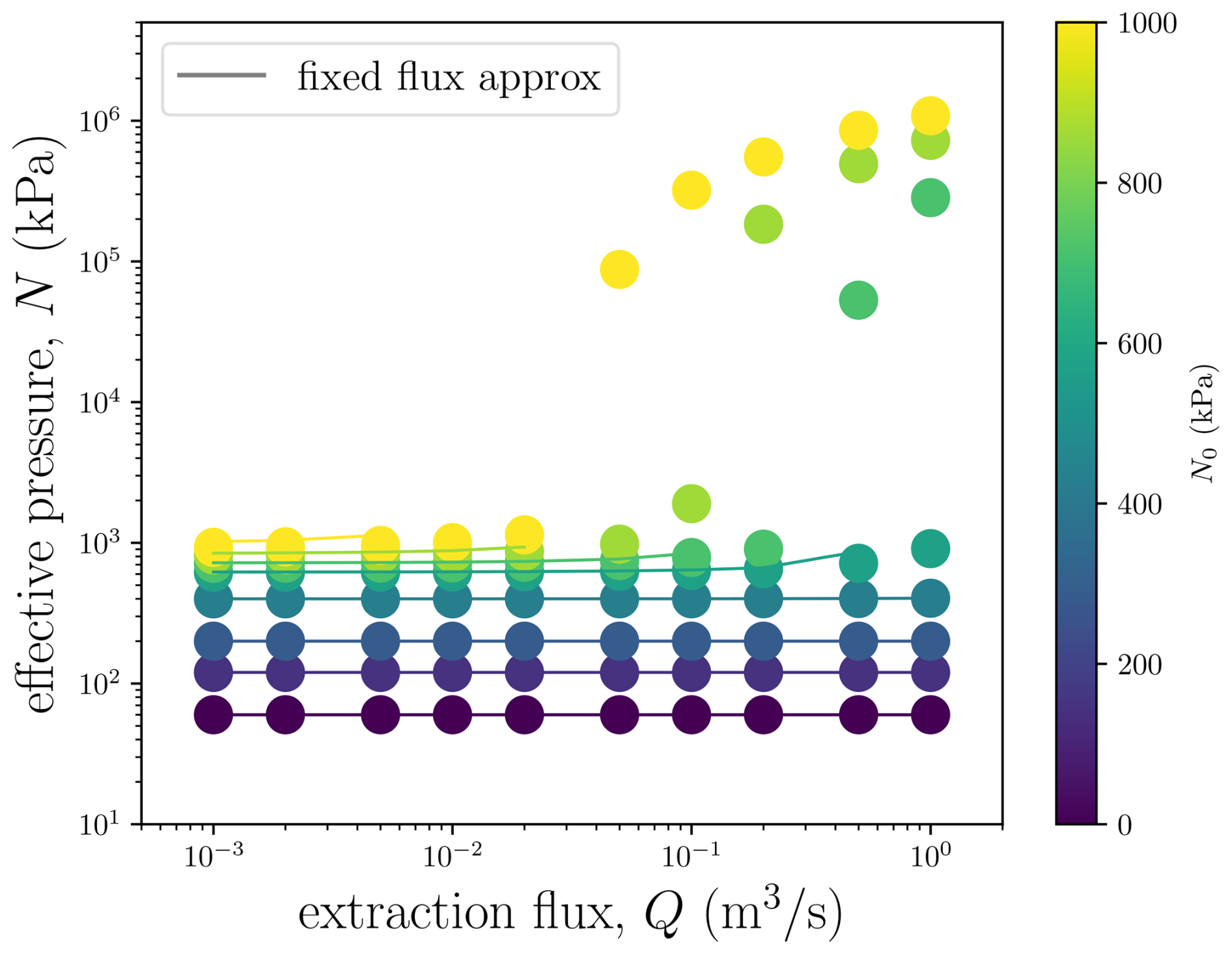
Figure 6 Varying flux solution for the effective pressure at the water extraction location, cf. Fig. B1. Each dot represents a simulation with a particular Q and N₀. The outer radius here is 10 km. The colored curves are the fixed flux approximate solutions from Eq. (B6), which do not yield a solution for large fluxes at high effective pressure.

By solving for the flux using this method, we can capture the effective pressure at the water extraction site as a function of the extraction flux Q and background effective pressure N₀, which we show in Fig. 6. For these steady state results, we find that larger values of each parameters produce elevated effective pressure at the borehole. If, however, the extraction flux or the effective pressure is small, the effective pressure is dominated by the background flow. This is important for connecting the results of the simplified axisymmetric model to the full SHAKTI simulations. We see that the varying flux model produces consistently slightly smaller effective pressures than the fixed flux model, but is able to capture the large effective pressure perturbations at high values of Q and N₀, where previously (i.e., in Fig. B1) there was a solution breakdown. Away from this regime, the colored curves, which show the approximate solution from Eq. (B6), agree well with the varying flux model for small N₀ and all Q as well as large N₀ and small Q, as in Fig. 4. Large pump systems could potentially be deployed on a glacier to pump on the order of 1–10 m³ s⁻¹, and these fluxes yield effective pressure changes on the order of 1–10 kPa. In the context of the chosen parameters, the effective pressure values are about 1 %–10 % of the background effective pressure, which is a small fraction of the total. These general predictions are for a steady state model that does not include positive feedbacks involving sliding, melt generation, and freezing.

3.3 Solution for constant gap height

Another relevant simplification of the dynamics of water extraction is to consider the case where the gap height is constant and fixed, b=β. Although this limit may appear artificial, it captures the initial pumping dynamics, i.e., before the system reaches a steady state. It is also relevant to the SHAKTI simulations of Helheim and Thwaites Glaciers, where a minimum gap height is imposed. In this constant gap height limit, Eq. (12) becomes

$$\begin{array}{}\text{(25)}& {\displaystyle \frac{\mathrm{d}N}{\mathrm{d}r}}=-{\displaystyle \frac{M}{{\mathit{\beta }}^{\mathrm{3}}}}\left({\displaystyle \frac{\mathrm{1}}{r}}+{\displaystyle \frac{R}{r^{\mathrm{2}}}}\right),\end{array}$$

where we have rearranged the terms and dropped the asterisks. In this case, since the gap height is fixed in time, and the effective pressure response will also be independent of time. Integrating and applying the boundary condition at the outer edge, i.e., N=1 at r=1, we find that

$$\begin{array}{}\text{(26)}& N=\mathrm{1}-{\displaystyle \frac{M}{{\mathit{\beta }}^{\mathrm{3}}}}\left(\ln \left(r\right)+R-{\displaystyle \frac{R}{r}}\right).\end{array}$$

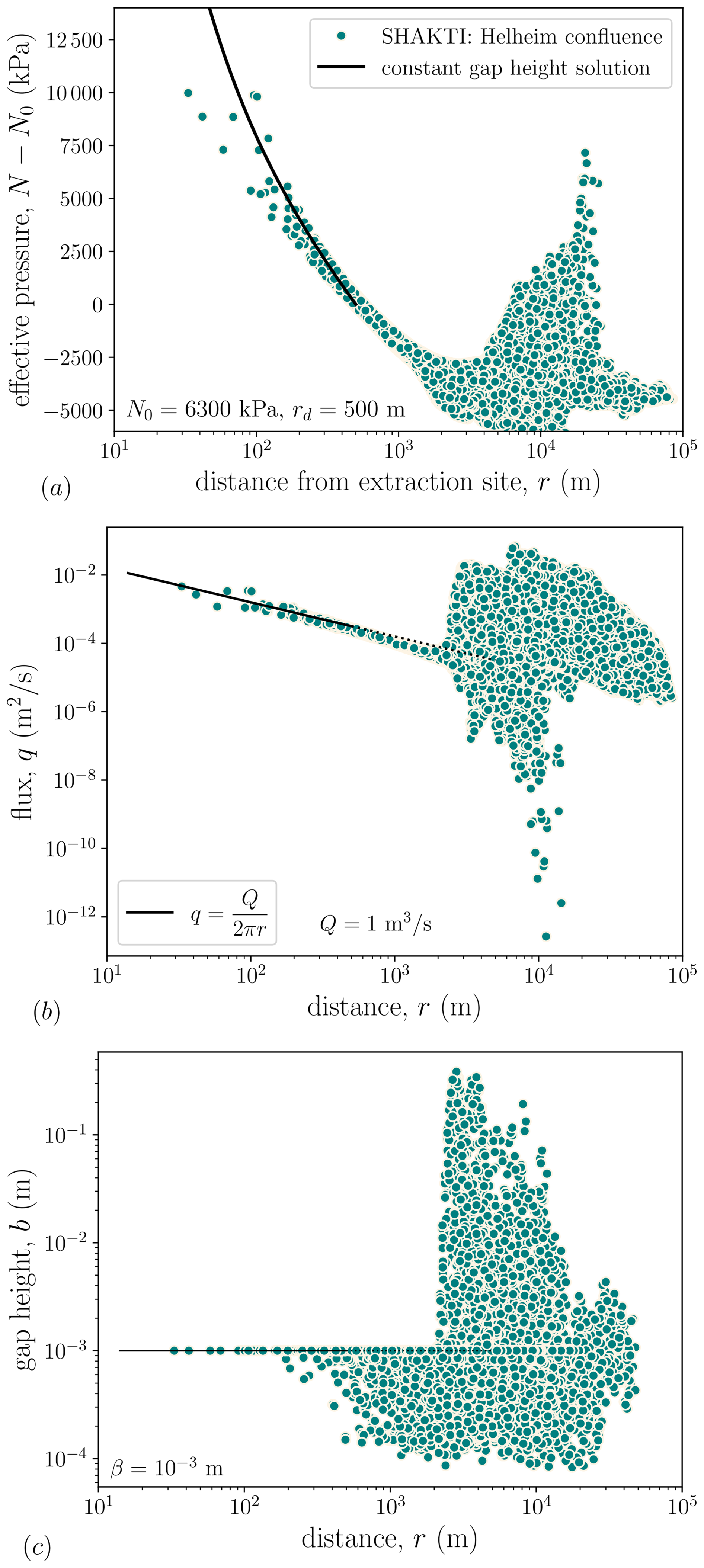
In this way, the effective pressure response is akin to a porous medium, where the β³ term represents a constant permeability. We plot the analytical solution for the effective pressure as a function of r in Fig. 7. The effective pressure near the point of extraction is significantly enhanced as compared to the background value.

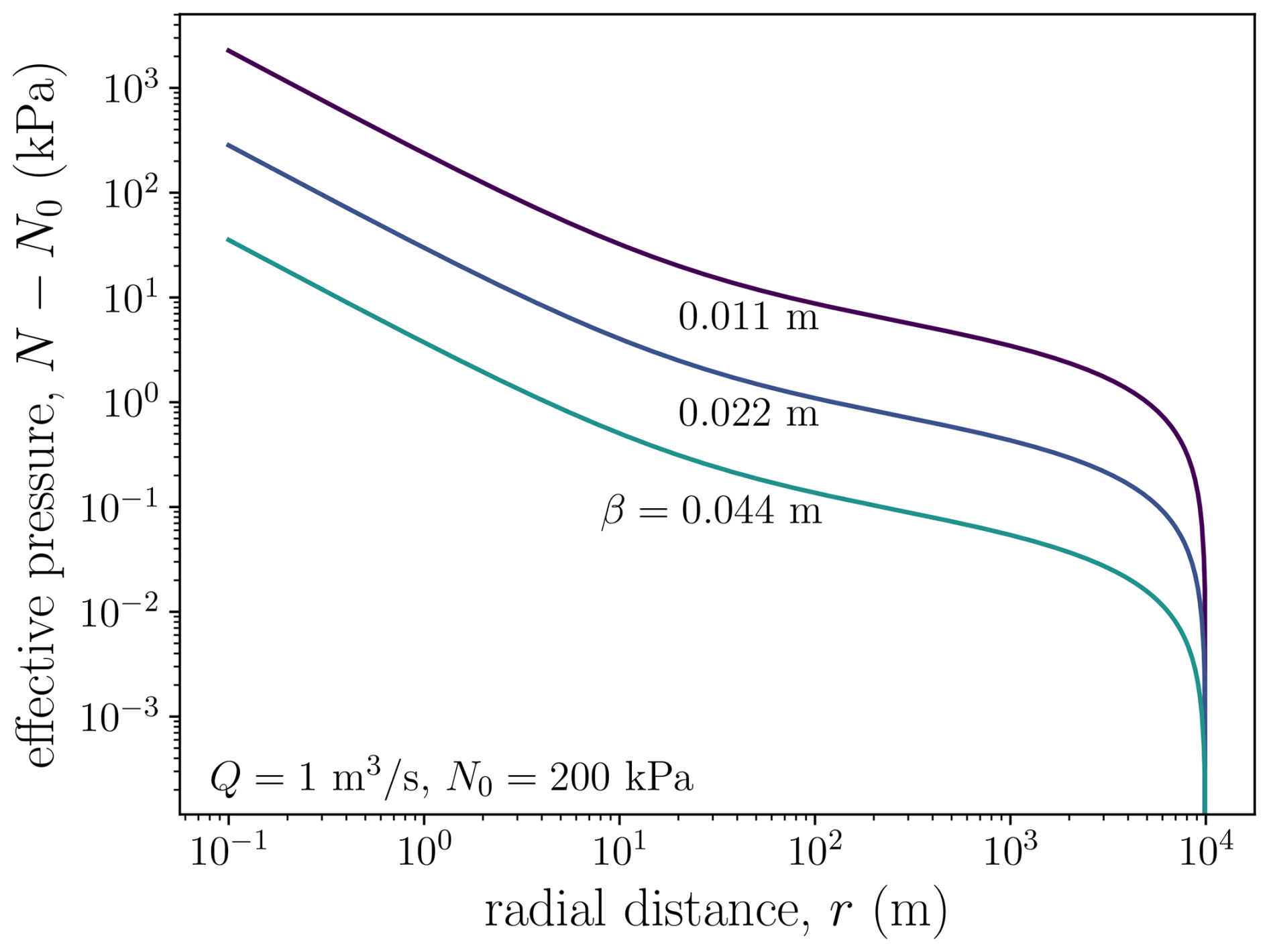
Figure 7 Effective pressure enhancement due to water extraction with a constant gap height. The domain is a 10 km circle and water is extracted from the center, with a flux given as $q=Q/\left(\mathrm{2}\mathit{\pi }r\right)$. For the smallest gap height shown, the effective pressure at the extraction site exceeds 1 MPa above the background value.

In Fig. 8, we revisit the SHAKTI pumping simulations in the confluence region of Helheim Glacier, Greenland, as shown in Fig. 2. We see that the constant gap height solution works well to explain the effective pressure near the water extraction site, due to the axisymmetric flux and fixed value of b. In SHAKTI-ISSM, we impose a minimum gap height for practical purposes. If the gap height is equal to this minimum, it will not shrink further, even if creep closure exceeds the melt opening rate. In practice, SHAKTI simulations do not always evolve the gap height in time and will stay at the minimum value. While we do not see a constant gap height as the best representation of the physics of the subglacial system, we leave further refinement of SHAKTI to future work. In the next section, we show that the connection between effective pressure and gap height is important in determining the effective pressure at the pumping location.

Figure 8 SHAKTI results and constant gap height model for the pumping tests in the confluence region of Helheim Glacier. (a) Effective pressure follows the analytical solution, Eq. (26) near the extraction site. (b) Flux decays like $Q/\left(\mathrm{2}\mathit{\pi }r\right)$. (c) The gap height is nearly constant close to the pump.

4 Influence of water extraction on ice velocity

We now return to the SHAKTI-ISSM simulations that sparked our interest in the axisymmetric problem: water extraction from model domains at Helheim Glacier, Greenland and Thwaites Glacier, Antarctica, where we use the same model and sliding law as described in Sect. 2. The question we aim to answer here is: what effect on velocity does pumping at multiple sites produce, compared to a single extraction site? We start by understanding the transient dynamics.

4.1 Time to steady state and extraction at the Helheim Glacier confluence

A pertinent question is how long is required for the subglacial system to respond fully to water extraction. From the time-dependent version of SHAKTI (Eq. 2; Sommers et al., 2018), the gap height evolves according to

$$\begin{array}{}\text{(27)}& {\displaystyle \frac{\partial b}{\partial t}}={\displaystyle \frac{\dot{m}}{{\mathit{\rho }}_{\mathrm{i}}}}-A{N}^{\mathrm{3}}b,\end{array}$$

where opening is caused by melt and closing is due to creep of the ice. In steady state, the two terms on the right are balanced, so that as steady state is approached both terms will have the same scaling, as described in Sect. 3. We find that the time to steady state is likely controlled by the creep closure timescale, i.e.,

$$\begin{array}{}\text{(28)}& \left[t\right]\sim {\displaystyle \frac{\mathrm{1}}{A{N}^{\mathrm{3}}}},\end{array}$$

which is the same scale we used to nondimensionalize the model in Sect. 3. Taking a representative effective pressure value of N₀∼1 MPa and the ice softness $A\simeq \mathrm{3.5}\times {\mathrm{10}}^{-\mathrm{25}}$ Pa⁻³ s⁻¹, the response timescale is on the order of

$$\left[t\right]\sim \mathrm{33}\text{d}.$$

For initial effective pressure values from, for example, 0.1–35 MPa, the timescale to reach steady state varies from ∼ 90 years to ∼ 1 min, with higher effective pressure corresponding to shorter response time. We expect that this scaling for time will also apply to the time for the system to recover (or “heal”) following cessation of water extraction. For times shorter than the Maxwell time for ice to relax (∼ 12 h, i.e., the timescale of applied forcing for ice to deform viscously rather than elastically; Ultee et al., 2020), this model for closure of subglacial gap height no longer applies. To account for these large effective pressure and rapid closure timescales, we would need to adapt SHAKTI to include elastic deformation. We leave this effort for future work, and consider the model here to be a first estimate for what could occur in this parameter regime.

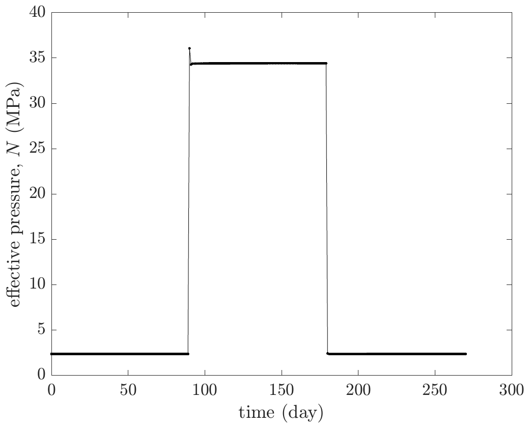
Figure 9 Change in effective pressure at the water extraction site over a pumping and recovery cycle at the “confluence point” of Helheim Glacier, Greenland (location shown in Fig. 10).

To examine these response times quantitatively, we performed a simulation over 270 d, with pumping at a steady rate of Q=1 m s⁻¹ applied at the confluence extraction site at Helheim during days 90–180, in order to demonstrate the response to pumping and the subsequent healing following the pumping period. As shown in Fig. 9, the effective pressure at the pumping site exhibits a short adjustment response to initiation and cessation of pumping. The expected timescale [t] from Eq. (28) for this simulation is ∼ 1 min, so it is unsurprising that the adjustment occurs quickly. We did not save every timestep in the SHAKTI simulations, indicating that the simulations are more resolved than the number of visible points. Figure 9 shows that the effective pressure returns to the same value after pumping. In Fig. 10, we see a change in effective pressure after 90 d of pumping. The largest impact is within a ring of about 2 km but variation in effective pressure is visible out to 5+ km away. In this coupled SHAKTI-ISSM simulation, the hydrology affects the ice velocity, which is also show on Fig. 10. The 90 d water extraction at the confluence leads to a slowdown on the order of 1 m yr⁻¹ throughout both branches. There are also a few patches of acceleration.

Figure 10 Pumping tests in the confluence region of Helheim Glacier, Greenland: (a) change in glacier velocity after 90 d of pumping at a rate of 1 m³ s⁻¹, and (b) change in effective pressure. The white asterisk indicates the location of the extraction site.

4.2 Water extraction from numerous sites at Helheim Glacier

Due to the physical and numerical limitations of extracting a large flux of water from a single borehole, we decided to model extracting water at Q=1 m³ s⁻¹ at 11 sites in the same 270 d pumping-and-healing experiment setup described in the previous section, with pumping employed during days 90–180, which we call the “pumping strategy”. Starting from the winter background state (i.e., no external water inflow, where all water at the bed is produced through basal melt), we then extract water from these 11 boreholes and allow the glacier velocity and subglacial hydrology to evolve in time, as shown in Fig. 12. The selected points are shown in Fig. 11. These points were chosen arbitrarily to be distributed along both branches and the main trunk of the glacier. There is intended overlap between some of these points and the locations analyzed by Sommers et al. (2024), where those authors show that terminus effects propagate ∼ 15 km upstream at Helheim. In the simulations here, neither the pumping strategy nor the location of the individual extraction sites were optimized to give the largest velocity change; we leave this type of detailed strategy design to future work.

Figure 11 Pumping tests on Helheim Glacier, Greenland: (a) location of 11 extraction sites overlaid on initial glacier velocity, (b) change in ice velocity after 90 d of pumping at a rate of 1 m³ s⁻¹ at each site, (c) change in effective pressure after 90 d of pumping, and (d) change in subglacial gap height after 90 d of pumping.

We find that our 11-point pumping strategy and model set up produce about 100 m yr⁻¹ slowdown in the main trunks of Helheim, as shown in Fig. 11. As a fraction of the total velocity, this influence is on the order of 1 % of the background velocity. We also only see deceleration, i.e., nowhere in the domain accelerates. In the Discussion (Sect. 6), we highlight areas of future work including longer simulations runs, seasonal effects, and pumping strategy optimization. For now, as a first test of the possibility of pumping water out to slow a glacier (as described by the model physics we incorporated), we can say that such an approach does yield a small velocity reduction.

In Fig. 12, we show the evolution of effective pressure with time for four representative sites. Similar to what we saw at the confluence site, the effective pressure at all sites returns to the same value as before pumping, indicating that pumping did not cause noise-induced drift (Robel et al., 2024). Some of the sites, however, do show evolution in the effective pressure during pumping. At one of the locations in the main trunk, we see a distinct transition in the effective pressure, indicative of a reconfiguration of the drainage network at that site caused by the water flow due to pumping, as shown in Fig. 11. At the far upstream site, the effective pressure oscillates before equilibrating to the a new steady state. These waves persist under time and space refinement, suggesting that they are not numerical artifacts but a transient reorganization of the drainage system. At other sites, a spike in effective pressure is apparent (i.e., Fig. 12), which is indicative of the constant gap height solution, as discussed in Sect. 3.3 and Fig. 7. The fast ice motion results in a large amount of meltwater generation at a large effective pressure, resulting in an unchanging gap height at some locations in the main trunk of Helheim (e.g., Fig. 11). In practice, this gap height remains fixed at the minimum allowable value imposed in the model and highlights the need for improved models of this critical component of glacier systems under low-flux conditions.

Figure 12 Change in effective pressure at 4 representative water extraction sites over a pumping and recovery cycle at Helheim Glacier. The left column shows the site locations at 4 times during the extraction period. The right column shows the effective pressure at the extraction site over time.

5 Simulations of Thwaites Glacier, Antarctica

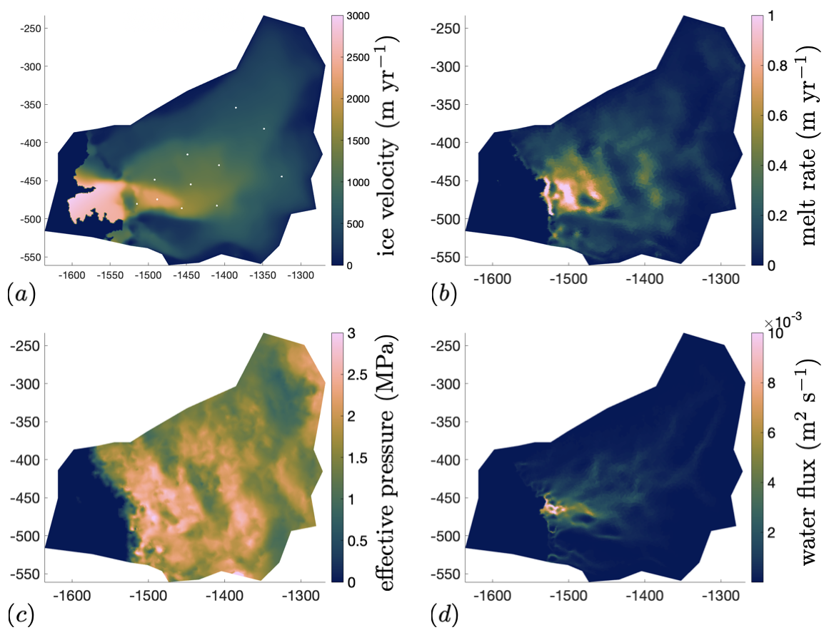
Figure 13 Simulating water extraction at Thwaites Glacier, Antarctica: (a) Modeled velocity of Thwaites Glacier resulting from an ISSM inversion using a Budd sliding law and subsequent coupled spin-up with the stress balance and subglacial hydrology. White dots indicate extraction sites. (b) Modeled subglacial melt rate. (c) Modeled effective pressure. (d) Modeled subglacial water flux, with the most significant fluxes approaching the grounding line.

We now turn to water extraction simulations at Thwaites Glacier, Antarctica, where we perform similar model experiments as at Helheim Glacier. We use the Thwaites domain set up from Goldberg et al. (2026). First, we run the coupled SHAKTI-ISSM model to steady state with no water inputs or extraction points using the Budd sliding law (see Appendix D for a comparison of the effects of different sliding laws). Modeled results are shown in Fig. 13. The background effective pressure falls in the range of N∼1–3 MPa, with highest subglacial water flux near the grounding line. These simulations are similar to the results using other subglacial hydrology models described in Hager et al. (2022) and Ehrenfeucht et al. (2025), where basal melt rate and water flux are highest near the grounding line. We then simulated extraction of water at rate of 1 m³ s⁻¹ at 11 randomly selected sites for 1 year. The 11 extraction points are shown in Fig. 13a and the results are shown in Fig. 14. This pumping strategy leads to a ∼ 10 m yr⁻¹ slowdown, which is about 1 % change in velocity in the main trunk. Again, we only see velocity reduction with no apparent zones of acceleration. These results are similar to what we saw when extracting water from 11 points at Helheim, in that both models led to a ∼ 1 % change in velocity and only produced slowdown. In future research, we will determine how transferrable this result is and whether it is robust across different subglacial hydrology models.

Figure 14 Impact of water extraction at Thwaites Glacier: (a) Velocity change in meters per year, showing a monotonic decrease. (b) Effective pressure change in Pa (n.b. 10⁵ Pa is 0.1 MPa). (c) Velocity change as a percentage of the total velocity in Fig. 13a, which is on the order of a 1 % decrease. (d) Effective pressure change as a percentage of effective pressure in Fig. 13c.

6 Discussion

In the context of using water extraction as a method to learn more about subglacial hydrology, our results provide predictions for the time to steady state, the effective pressure at the extraction site, and radius of influence. These predictions could be used in the design of laboratory experiments involving numerous boreholes spaced out radially, with water extracted from a central borehole (e.g., Zoet and Iverson, 2016, 2020; Hansen et al., 2024). The measured effective pressure distribution would allow us to compare the shape of the curve to our prediction and determine the parameters for the best-fit values of $D,M,W,\text{and}R$. It is also possible that these experiments could demonstrate that our model does not represent the dominant physics, and the radial distribution of effective pressure could take a different form. This outcome would result in a helpful reformulation of subglacial hydrology and provide context for comparison to experiments, similar to the determination of the effective film thickness by Engelhardt and Kamb (1997).

In our predictions for the effect of water extraction on glacier velocity, we did not include seasonal dynamics (e.g., surface meltwater draining to the bed), nor did we include multi-year impacts, and we did not optimize the location of the extraction points. While we leave these extensions to future work, it is worth discussing how they may affect the results. First, the seasonal water input from surface melting at Helheim is immense (on the order of 1 km³; Stevens et al., 2022a) and water extraction would have a difficult time competing: it would take ∼ 32 years for a single borehole with Q=1 m³ s⁻¹ to extract the surface melting of a single season. Future simulations could include surface water input and examine the most effective time period to pump. It is clear that the pumping strategy affects the relationship between water extraction and glacier slowdown, yet the simulations presented here are intended to be illustrative of the overall concept and we did not optimize the locations of extraction, the timing, or the pumping rate. For example, all of the locations in the main trunks of Helheim and Thwaites have only a small effect on the resulting velocity (cf. Figs. 11 and 13). This makes sense given the Sommers et al. (2024) results, which showed that hydrology is most influential in the upstream regions, i.e., away from the coast and out of the fast flowing sectors. On longer timescales and over repeated seasons of water extraction, feedbacks related to sliding and freezing to the bed could kick in. Water piracy is hypothesized to be the cause of the Kamb Ice Stream stagnation in Antarctica (e.g., Alley et al., 1994) and could affect the long-term evolution of glaciers such as Helheim and Thwaites if water is extracted. Freezing to the bed due to slowing glacier velocity would be more effective at reducing glacier flux than extracting water alone (Tulaczyk et al., 2000; Robel et al., 2013; Meyer et al., 2018, 2019). Further research could optimize locations of water extraction (focusing on the upstream reaches) and run multi-year simulations, where increases in basal traction could lead to flow reorganization.

In this work, we did not consider the practical question that arises of what becomes of the extracted water. Possibilities include making snow (during winter pumping when air temperatures are consistently below freezing) or injecting the extracted water down an existing moulin (during a summer deployment with seasonal surface melting), aiming to enhance an existing efficient subglacial channel, draining pressure from the surrounding bed. Nor did we consider engineering considerations for such a pumping strategy to be implemented, the cost-benefit analysis, or the ethical and moral considerations of such an approach. This we leave for future studies, for which this present work may provide some constraints on the scale of intervention required.

As a glacier intervention strategy, our SHAKTI-ISSM numerical results suggest that water extraction can act to modestly slow glaciers in a model system. With attainable pumping rates over a reasonable time span and a drilling campaign that has precedent in the literature (e.g., Kamb, 2001), in a model that encodes our knowledge of ice and water flow physics, we find a small slowdown of Helheim and Thwaites Glaciers, among the fastest-flowing glaciers on planet Earth. Water extraction did not stop Helheim and Thwaites in their tracks and more research is required to understand the mechanics by which water extraction could significantly slow these glaciers. For the simulations of Helheim Glacier, we built on an existing model configuration (Sommers et al., 2023, 2024) and only considered wintertime pumping. Glacier intervention in Greenland would need to contend with the large amounts of seasonal surface meltwater and rapid glacier flow. For comparison, we also included simulations of Thwaites Glacier, Antarctica, which is an important glacier for sea-level rise, flows more slowly than Helheim, and does not currently experience surface melt. Our results show a similar ∼1 % change in ice velocity at both glaciers, as a consequence of water extraction at 11 arbitrary points on each. More research is required before we can determine if water extraction is an effective intervention strategy resulting in a meaningful slowdown of mass loss from the polar ice sheets. Regardless, the research spurred by this line of inquiry will improve subglacial hydrology models to improve accuracy of future sea-level change projections.

7 Conclusions

Changes in subglacial water flux and pressure affect glacier velocity. In this paper, we analyzed the effects of water extraction on glacier velocity. We started by considering axisymmetric subglacial water flow around a single borehole. We developed a model and used this framework to answer three key questions about the radius of influence, the extraction pressure, and the timescale of evolution. We found that the effective pressure perturbations had a logarithmic component, allowing the effective pressure to stay elevated far away from the borehole. We determined the relationship between extraction flux and extraction effective pressure. We showed that creep closure dominates the time it takes for the pumping to reach steady state and similarly recover following pumping, with typical response times on the order of days. Building off these results, we presented coupled subglacial hydrology–ice dynamics simulations of Helheim Glacier, Greenland and Thwaites Glacier, Antarctica using SHAKTI-ISSM. We found that the velocity reduced about 1 % for a reasonable pumping strategy. Overall, we demonstrate the utility of studying water extraction as a way to learn more about the subglacial hydrologic system as well as to determine its efficacy as a glacier intervention strategy.

Appendix A: Asymptotic solution for a small extraction flux

Figure A1 Asymptotic solution for a small extraction flux: (a) Flux with distance, showing a transition to the small q solution. (b) The small flux solution for the effective pressure agrees with the full solution.

In Fig. 4, we observed that for small extraction fluxes, that fluid can enter from the outer edge of the domain. We can describe these dynamics in the asymptotic limit of a small extraction flux and ignore dissipation, i.e., M≪1, R≪1, W≫1, and D=0. In this distinguished limit, we can reduce Eqs. (11)–(14) to

$$\begin{array}{}\text{(A1)}& {\displaystyle }Mq\left(\mathrm{1}+Rq\right)=-N^{-\mathrm{9}}{\displaystyle \frac{\mathrm{d}N}{\mathrm{d}r}},\text{(A2)}& {\displaystyle \frac{\mathrm{1}}{r}}{\displaystyle \frac{\mathrm{d}}{\mathrm{d}r}}\left(rq\right)=-W.\end{array}$$

We now integrate mass conservation to determine the flux as

$$\begin{array}{}\text{(A3)}& q=-{\displaystyle \frac{\mathrm{1}}{\mathrm{2}}}Wr,\end{array}$$

where we take the constant of integration that comes from setting the inner boundary condition to be zero, since W is large. Inserting the flux into Eq. (A1), we find that

$$\begin{array}{}\text{(A4)}& -\mathrm{4}MWr+\mathrm{2}R{W}^{\mathrm{2}}M{r}^{\mathrm{2}}={\displaystyle \frac{\mathrm{d}}{\mathrm{d}r}}\left(N^{-\mathrm{8}}\right).\end{array}$$

Integrating and applying the outer boundary condition, N=1 at r=1, gives

$$\begin{array}{}\text{(A5)}& N={\left[\mathrm{1}+\mathrm{2}MW\left(\mathrm{1}-r^{\mathrm{2}}\right)-{\displaystyle \frac{\mathrm{2}}{\mathrm{3}}}R{W}^{\mathrm{2}}M\left(\mathrm{1}-r^{\mathrm{3}}\right)\right]}^{-\mathrm{1}/\mathrm{8}},\end{array}$$

which is shown in Fig. A1. The asymptotic model agrees with the full flux model. The minimum effective pressure is given by

$$\begin{array}{}\text{(A6)}& N_{\text{min}}={\left[\mathrm{1}+\mathrm{2}MW-{\displaystyle \frac{\mathrm{2}}{\mathrm{3}}}R{W}^{\mathrm{2}}M\right]}^{-\mathrm{1}/\mathrm{8}}.\end{array}$$

This solution works well for small fluxes, as shown in Fig. A1. The dimensionless groups that arise in this solution are given by

$$\begin{array}{ll}{\displaystyle }& {\displaystyle }MW={\displaystyle \frac{\mathrm{12}\mathit{\mu }{r}_{\mathrm{d}}}{[b{]}^{\mathrm{3}}{N}_{\mathrm{0}}}}{\displaystyle \frac{\left(G+u_{\mathrm{b}}{\mathit{\tau }}_{\mathrm{b}}\right)r_{\mathrm{d}}}{{\mathit{\rho }}_{\mathrm{w}}\mathcal{L}}}\text{and}\\ {\displaystyle }& {\displaystyle }R{W}^{\mathrm{2}}M={\displaystyle \frac{\mathrm{12}\mathit{\omega }{\mathit{\rho }}_{\mathrm{i}}{\mathit{\rho }}_{\mathrm{w}}\mathcal{L}{A}^{\mathrm{3}}{N}_{\mathrm{0}}^{\mathrm{8}}{r}_{\mathrm{d}}^{\mathrm{3}}}{\left(G+u_{\mathrm{b}}{\mathit{\tau }}_{\mathrm{b}}\right)}},\end{array}$$

which are independent of the flux Q. The first group can be seen as a ratio of the flux generated from melting due to sliding and geothermal heat to the expected flux through the system. The second term determines the role of turbulent melting in the system as compared to geothermal heat and sliding.

Returning to the step above where we set the inner boundary condition to zero, this choice is not required and we can derive a more general analytical solution by including the inner flux. In this way, we find that

$$\begin{array}{}\text{(A7)}& q=-{\displaystyle \frac{\mathrm{1}}{\mathrm{2}}}Wr+{\displaystyle \frac{\mathrm{1}}{r}}.\end{array}$$

Inserting this flux into Eq. (A1), we find that

$$\begin{array}{}\text{(A8)}& \begin{array}{rl}{\displaystyle \frac{M}{r}}& +{\displaystyle \frac{MR}{r^{\mathrm{2}}}}-MWR-{\displaystyle \frac{\mathrm{1}}{\mathrm{2}}}rWM\\ & +{\displaystyle \frac{\mathrm{1}}{\mathrm{4}}}{r}^{\mathrm{2}}M{W}^{\mathrm{2}}R={\displaystyle \frac{\mathrm{1}}{\mathrm{8}}}{\displaystyle \frac{\mathrm{d}}{\mathrm{d}r}}\left(N^{-\mathrm{8}}\right).\end{array}\end{array}$$

Upon integrating and applying the outer boundary condition, we find that

$$\begin{array}{}\text{(A9)}& \begin{array}{rl}N& =\left\{\mathrm{1}+\mathrm{8}M\left[\ln \left(r\right)+R\left(\mathrm{1}-{\displaystyle \frac{\mathrm{1}}{r}}\right)+WR(\mathrm{1}-r)\right.\right.\\ & {\left.\left.+{\displaystyle \frac{\mathrm{1}}{\mathrm{4}}}W\left(\mathrm{1}-r^{\mathrm{2}}\right)-{\displaystyle \frac{\mathrm{1}}{\mathrm{12}}}{W}^{\mathrm{2}}R\left(\mathrm{1}-r^{\mathrm{3}}\right)\right]\right\}}^{-\mathrm{1}/\mathrm{8}},\end{array}\end{array}$$

which is a combination of the earlier analytical solution that neglects dissipation, i.e., Eq. (22), and the small-flux asymptotic solution just described, Eq. (A5). This solution extends the applicability of the small flux asymptotics to larger values of M, R, and smaller values of W.

Appendix B: Numerical and approximate solutions to the fixed flux model

B1 Shooting and relaxation methods when including dissipation

Starting with Eqs. (16)–(18), in Sect. 3.1.1, we ignored the effect of turbulent dissipation on melting, which becomes important as q increases towards the borehole. If we now include dissipation, we must solve the equations numerically, which we can do using a relaxation method. We use forward Euler to march the gap height b forward in time, then use the value of the gap height at the previous time step to find $\partial N/\partial r$ from the equation for the water flux. We then use $\partial N/\partial r$ to find the melt rate, and use that expression to move forward in time and update b.

In steady state, we have the reduced equations given by

$$\begin{array}{}\text{(B1)}& M\left({\displaystyle \frac{\mathrm{1}}{r}}+{\displaystyle \frac{R}{r^{\mathrm{2}}}}\right)=-b^{\mathrm{3}}{\displaystyle \frac{\partial N}{\partial r}},N^{\mathrm{3}}b=\mathrm{1}-{\displaystyle \frac{D}{r}}{\displaystyle \frac{\partial N}{\partial r}}.\end{array}$$

We can combine these into a single ODE for $\partial N/\partial r$ as

$$\begin{array}{}\text{(B2)}& {\left[\mathrm{1}+{\displaystyle \frac{D}{r}}\left(-{\displaystyle \frac{\partial N}{\partial r}}\right)\right]}^{\mathrm{3}}\left(-{\displaystyle \frac{\partial N}{\partial r}}\right)={\displaystyle \frac{M}{r}}\left(\mathrm{1}+{\displaystyle \frac{R}{r}}\right)N^{\mathrm{9}},\end{array}$$

where we solve for $-\partial N/\partial r$ using a root-finding algorithm and then integrate backward starting from N=1 at r=1.

B2 Approximate solution for effective pressure at extraction location

In the main text, we show the effective pressure at the extraction site using the full varying flux model, i.e., Fig. 6. As an approximate model, we could use a fixed flux and numerically solve the steady ODE that includes turbulent dissipation, i.e., Eq. (B2). We know from Fig. 4 that this solution has an internal singularity for large values of the background effective pressure N₀, and this solution breakdown is discussed more in Appendix C. For small values of N₀, however, the fixed flux steady ODE is a reasonable model. Including dissipation regularizes the singularity in the analytical solution Eq. (22) and the near-field effective pressure approaches a constant. In Fig. B1, we show the steady ODE solution to the problem, showing the approach to a constant in the near field, the singularity in the approximate analytical expression, and the logarithmic decay behavior in the far field. There is a boundary layer for small r where turbulent dissipation dominates, the gap height opens due to enhanced melting, and the effective pressure is more or less constant. Matching this inner region to the approximate analytical outer solution, Eq. (22), proved intractable analytically, in part because of the singularity at finite r. To capture the essence of the behavior, we noticed that the value of effective pressure for the outer solution at the point where the dissipation is order unity, i.e.,

$$\begin{array}{}\text{(B3)}& -{\displaystyle \frac{D}{r}}{\displaystyle \frac{\mathrm{d}N}{\mathrm{d}r}}\sim \mathrm{1},\end{array}$$

is close to the value of the inner solution. In this region, we assume that r<R, so that the effective pressure and its gradient are approximately given as

$$\begin{array}{}\text{(B4)}& N\simeq \mathrm{1}+{\displaystyle \frac{MR}{r}}\text{and}{\displaystyle \frac{\mathrm{d}N}{\mathrm{d}r}}\simeq -{\displaystyle \frac{MR}{r^{\mathrm{2}}}}.\end{array}$$

This implies that the dissipation term is order unity when the radius r is approximately

$$\begin{array}{}\text{(B5)}& r\simeq {\left(DMR\right)}^{\mathrm{1}/\mathrm{3}}.\end{array}$$

We then evaluate the outer effective pressure analytical expression at this radius and find that

$$\begin{array}{}\text{(B6)}& N\simeq \mathrm{1}+{\left({\displaystyle \frac{M^{\mathrm{2}}{R}^{\mathrm{2}}}{D}}\right)}^{\mathrm{1}/\mathrm{3}}\end{array}$$

As shown in Fig. 6, this approximate approach agrees well with the full solution for low Q and N₀.

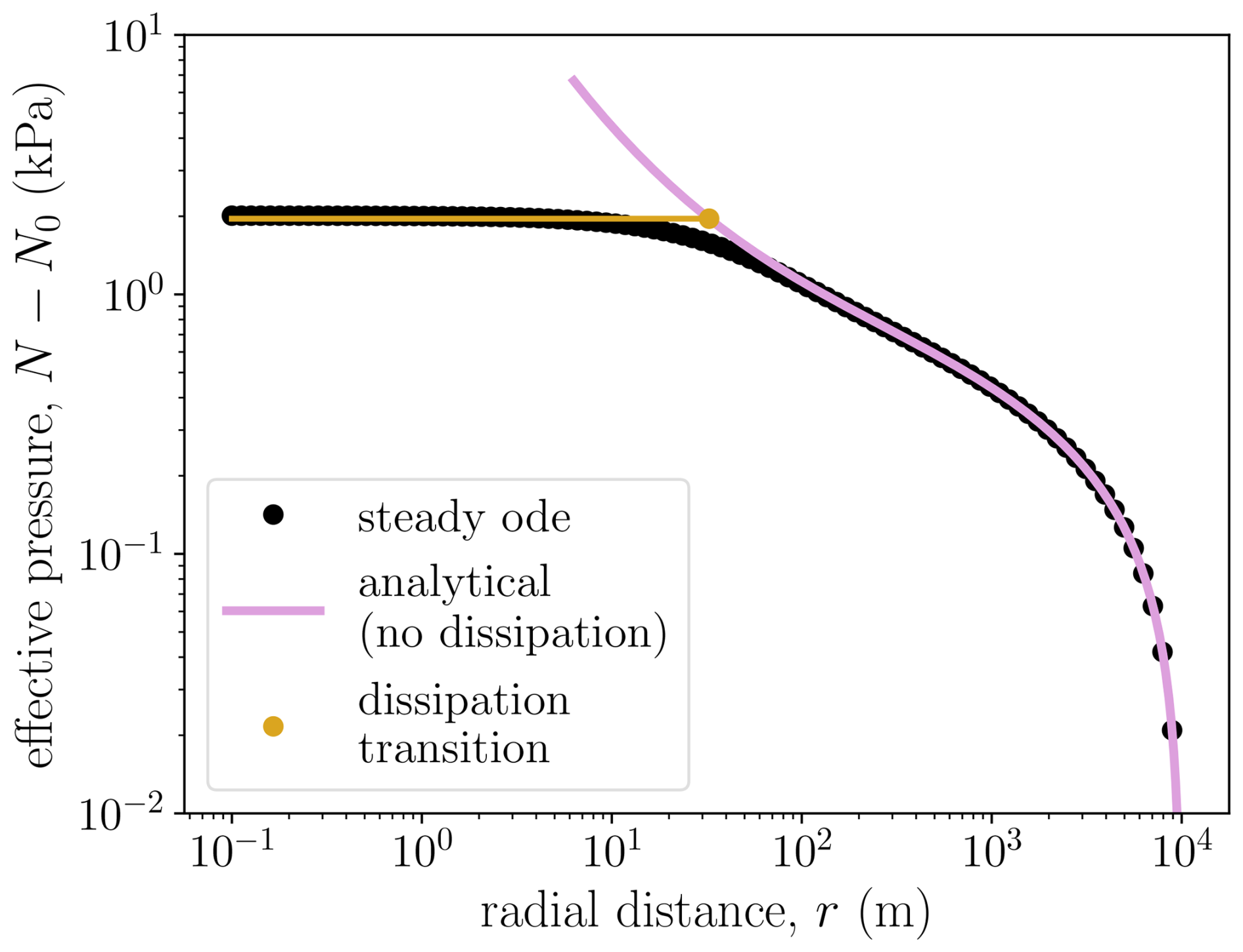
Figure B1 In steady state, extracting water increases the local effective pressure by stimulating water flow: effective pressure as a function of radial distance, showing the analytical solution where we ignore dissipation. By finding the radius where turbulent dissipation is significant, we approximate the effective pressure at the borehole (gray curves) from Eq. (B6).

Appendix C: Pressure divergence at high pumping rates

As the value of the outer effective pressure becomes larger in Fig. B1, there is a breakdown in the numerical solution, which almost uniformly occurs for large effective pressures (i.e., a singularity inside the domain, as shown in Fig. 4). To understand this breakdown, we look for the domain of applicability for Eq. (B2). To start, we can see that as the effective pressure at the outer boundary increases, the hydraulic permeability of the domain decreases. For a fixed form of the flux $q=Q/\mathrm{2}\mathit{\pi }r$, this means the pressure gradient towards the borehole must increase to maintain the imposed value of Q, further increasing N and decreasing the gap height and permeability. If the outer boundary pressure is too large for the flux imposed, the effective pressure diverges before the before we reach r=0. Physically, this corresponds to a hydrological system that collapses in on itself from the induced pressure gradients, like a straw collapsing shut. Indeed, for any value of Q and domain size r_d we can find the maximum N₀ at the boundary such that this divergence occurs exactly at r=0. Since $\partial N/\partial r$ is only a function of N and r, considering this as a 2D dynamical system, curves of N(r) cannot intersect, so any solutions with a lower value of N₀ will remain bounded as r→0 and any with a larger value of N₀ will diverge at finite r. Practically, it is easiest to integrate outwards from r=0, and continue along this bounding curve, which we refer to as the envelope, to reach any value of r_d.

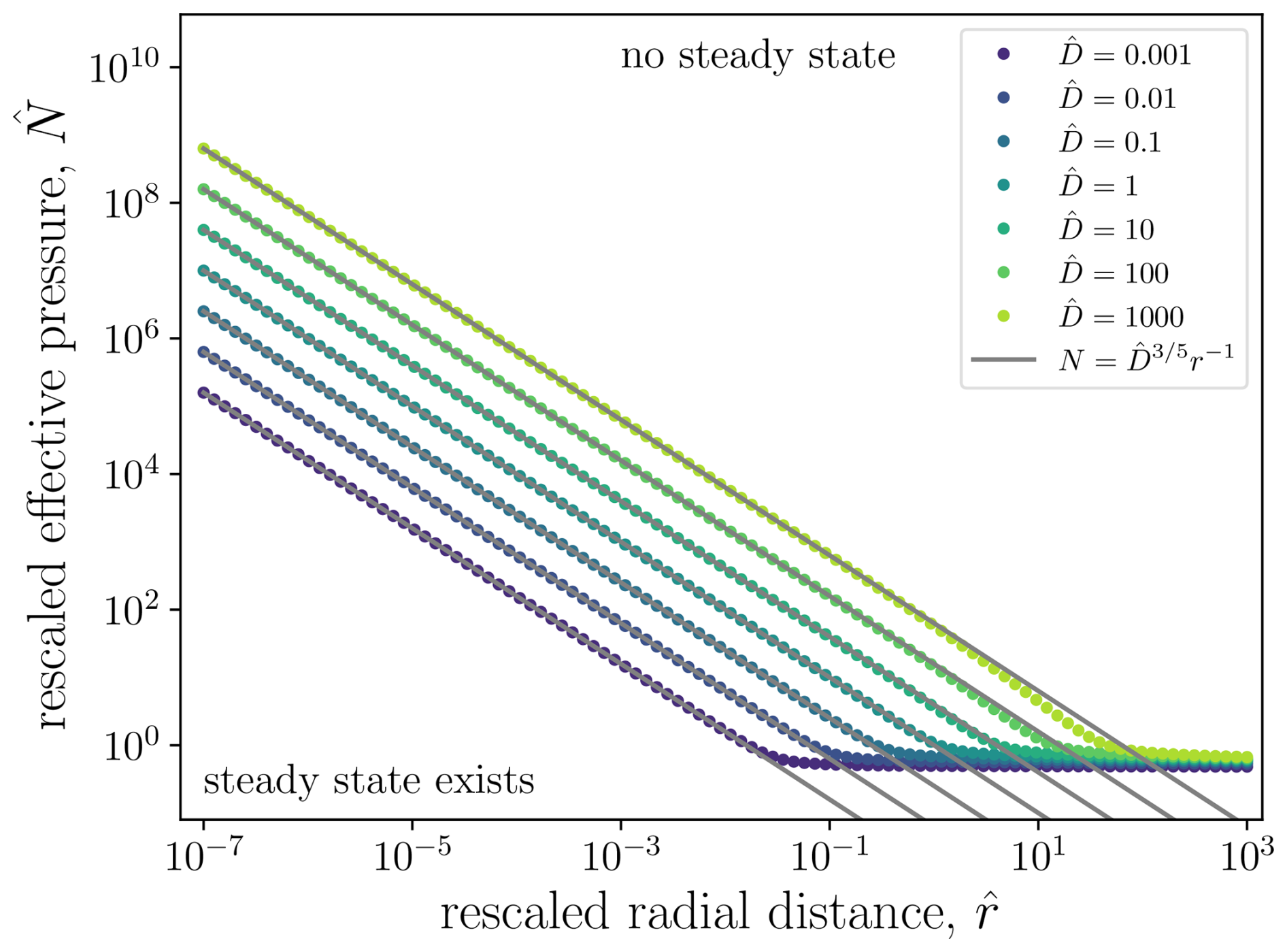
Figure C1 Curves of maximum steady state effective pressure as a function of radial distance and a unified dissipation parameter $\widehat{D}$. Choosing initial conditions at a radius below the curve for a given $\widehat{D}$ result in a steady solution, whereas steady solutions above the curve do not exist.

We start by rescaling the variables so that

$$\begin{array}{ll}{\displaystyle }& {\displaystyle }r=R\widehat{r},N=M^{-\mathrm{1}/\mathrm{8}}\widehat{N},\text{and}\\ {\displaystyle }& {\displaystyle }\widehat{D}={\displaystyle \frac{D}{R^{\mathrm{2}}{M}^{\mathrm{1}/\mathrm{8}}}}={\displaystyle \frac{(\mathrm{2}\mathit{\pi }{)}^{\mathrm{9}/\mathrm{8}}{\mathit{\nu }}^{\mathrm{2}}}{\left(\mathrm{12}\mathit{\mu }{)}^{\mathrm{1}/\mathrm{8}}\right({\mathit{\rho }}_{\mathrm{i}}LA{)}^{\mathrm{3}/\mathrm{8}}(G+u_{\mathrm{b}}{\mathit{\tau }}_{\mathrm{b}}{)}^{\mathrm{5}/\mathrm{8}}{\mathit{\omega }}^{\mathrm{2}}{Q}^{\mathrm{9}/\mathrm{8}}}},\end{array}$$

which is independent of N₀ and r_d. This rescaling leads to a one-parameter version of Eq. (B2), i.e.,

$$\begin{array}{}\text{(C1)}& {\left[\mathrm{1}+{\displaystyle \frac{\widehat{D}}{r}}\left(-{\displaystyle \frac{\partial \widehat{N}}{\partial \widehat{r}}}\right)\right]}^{\mathrm{3}}\left(-{\displaystyle \frac{\partial \widehat{N}}{\partial \widehat{r}}}\right)={\displaystyle \frac{\mathrm{1}}{\widehat{r}}}\left(\mathrm{1}+{\displaystyle \frac{\mathrm{1}}{\widehat{r}}}\right){\widehat{N}}^{\mathrm{9}},\end{array}$$

which has an asymptotic solution for small $\widehat{r}$ of $\widehat{N}\simeq {\widehat{D}}^{\mathrm{3}/\mathrm{5}}{\widehat{r}}^{-\mathrm{1}}$. We integrate Eq. (C1), starting from a very large effective pressure at the extraction site (i.e., $\widehat{N}=D^{\mathrm{3}/\mathrm{5}}/\mathit{ϵ}$ at $\widehat{r}=\mathit{ϵ}$ with ϵ→0) and find that the curve locks onto the largest steady state effective pressure for given values of $\widehat{r}$ and $\widehat{D}$. The result of this integration is shown in Fig. C1. The different curves on the plot in Fig. C1 represent different values for the parameter $\widehat{D}$, corresponding different extraction fluxes Q, and parameters such as ice softness A and geothermal heat G. From this analysis, we can see that if we impose N=N₀ at a radius r=r_d and that the point falls above the curve for the associated value of $\widehat{D}$, then there will not be a steady state solution. It is for this reason that large N₀ and large Q resulted in singularities in Fig. B1. Part of the reason that we find a region of parameter space that does not have a steady state is that we have neglected mass conservation, i.e., Eq. (5), by assuming that $q=Q/\left(\mathrm{2}\mathit{\pi }r\right)$ and neglecting the right hand side of this equation. As the melt rate increases, due to larger Q or $\mathrm{d}N/\mathrm{d}r$, this approximation is no longer viable.

Appendix D: Effect of sliding law on water extraction experiments

Using the Thwaites Glacier domain as a testbed, here we compare the results of water extraction with Budd sliding, e.g., Fig. 13, with those using a regularized Coulomb sliding law. The equations for the two sliding laws are given as

$$\begin{array}{}\text{(D1)}& {\displaystyle }{\mathit{\tau }}_{\mathrm{b}}=C^{\mathrm{2}}{u}_{\mathrm{b}}N\text{(Budd)},\text{(D2)}& {\displaystyle }{\mathit{\tau }}_{\mathrm{b}}={\displaystyle \frac{{\mathit{\alpha }}^{\mathrm{2}}{u}_{\mathrm{b}}^{\mathrm{1}/\mathrm{3}}}{{\left[\mathrm{1}+{\left(\frac{\mathrm{2}{\mathit{\alpha }}^{\mathrm{2}}}{N}\right)}^{\mathrm{3}}{u}_{\mathrm{b}}\right]}^{\mathrm{1}/\mathrm{3}}}}\text{(regularized Coulomb)},\end{array}$$

where the unknown coefficient in the regularized Coulomb law is α. The physics encoded in the regularized Coulomb allows for rate-strengthening at sliding velocities when the stress is below a yield stress and converges to Coulomb friction at higher velocities (Schoof, 2005; Joughin et al., 2019; Zoet and Iverson, 2020; Helanow et al., 2021; Hansen et al., 2024).

In Fig. D1, we compare the results of the 11-point, 1-year pumping experiment at Thwaites for the two different sliding laws. We see that the Budd sliding law leads to a larger change in velocity. While a small difference between the two results come from the fact that the inverted velocities are similar but not exactly the same, the majority of the difference arises because of the influence of effective pressure on the sliding law. In the Budd sliding law case, the basal shear stress is directly proportional to the change in effective pressure. A 5 % increase in N will require a similar percentage decrease in u_b to maintain the same τ_b. For regularized Coulomb, the basal shear stress is less sensitive to effective pressure because the background effective pressure is large, as shown in Fig. 13. In this limit where the shear stress is below the yield stress, the sliding law is dominated by the rate-strengthening component, and changes in the effective pressure have a muted effect on the sliding speed. Without data to constrain the effective pressure, we speculate that at smaller background effective pressures, we would see a larger velocity change. Our results show that (i) the choice of sliding law is important for determining the velocity change; (ii) the subglacial hydrology model sets the magnitude of the effective pressure, which influences the parameter regime in the sliding law; and (iii) further research into constraining sliding laws, effective pressures, and basal velocities at Thwaites will directly inform the predicted velocity reduction.

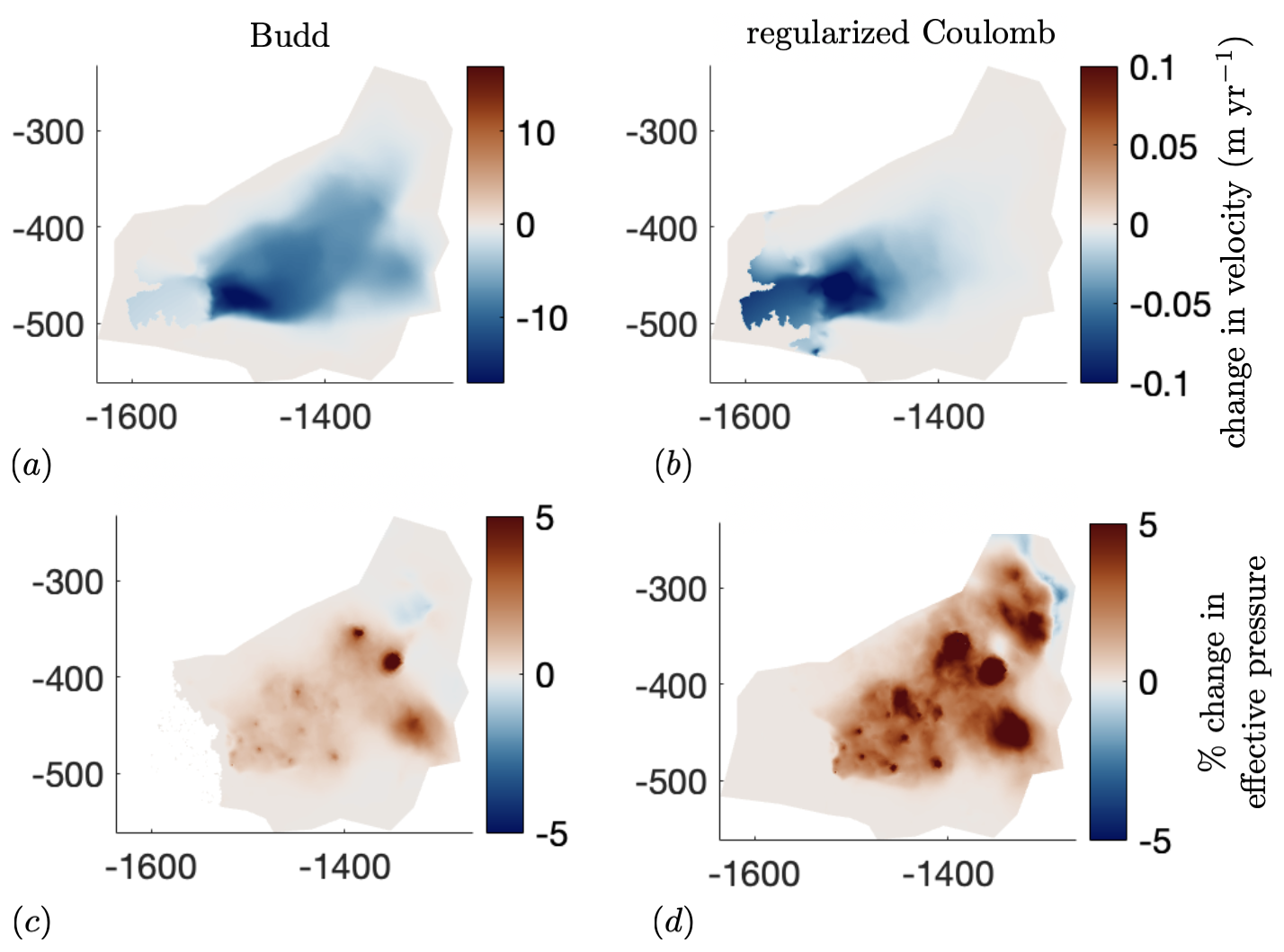
Figure D1 A comparison between the velocity change at Thwaites after one year of pumping with two different sliding laws: (a) Velocity change with a Budd sliding law. (b) Velocity change with a regularized Coulomb sliding law. (c) Percent change in effective pressure with a Budd sliding law. (d) Percent change in effective pressure with a regularized Coulomb sliding law.