The Eurasian and North American ice sheets at the Last and Penultimate glacial maxima: coupled atmosphere–ice sheet model sensitivity and calibration

The configuration of the Northern Hemisphere ice sheets during the Last and Penultimate Glacial Maxima (LGM; PGM) influenced millennial-scale climate changes, as well as solid Earth and sea level changes that occurred during the subsequent deglaciations, due to their effects on the atmosphere, ocean circulation, and the solid Earth. Thus, realistic simulations of these ice sheets are crucial for the initialisation of deglaciation experiments that can help improve our understanding of interactions between the climate, ice sheets and sea levels. Here, we produce the first large ensembles of complex coupled atmosphere–ice sheet model (FAMOUS-BISICLES) simulations of the PGM and LGM, varying 12 uncertain parameters that control the ice sheet albedo, ice dynamics and climate. We quantify the sensitivity to input parameters using Gaussian Process emulators to perform a Sobol sensitivity analysis. Albedo parameters have the largest influence on ice volumes for both ice sheets and time periods. Parameters controlling precipitation and sliding have a larger effect on Eurasian than North American ice sheet size due to the differences in geographical and climatic settings. Out of 120 parameter combinations, we find 4 that produce LGM and PGM ice volumes and extents compatible with palaeo-evidence. The resulting ice sheet configurations provide new and improved reconstructions of PGM Northern Hemisphere ice sheets for use as inputs in climate, ice sheet and sea level models.

1 Introduction

During the last 800 000 years, glacial periods saw the accumulation of large ice sheets over the Northern Hemisphere (NH) continents (Ehlers et al., 2018). Their size, shape, and evolution exerted a strong influence on the climate through their interactions with atmospheric and oceanic circulation, as well as the energy budget (Beghin et al., 2015; Fyke et al., 2018; Izumi et al., 2023; Roberts et al., 2019). Thus, reconstructing their extent and thickness is key to deciphering the causes of past climatic and environmental changes.

Beyond impacting the energy balance through their high albedo, ice sheets have direct effects on ocean circulation, atmospheric circulation, and precipitation patterns. They affect deep water formation and circulation in the North Atlantic, either through their freshwater release near sites of deep water formation, their impact on energy balance, or their effect on wind patterns (Gregoire et al., 2018; Sherriff-Tadano et al., 2018, 2021; Smith and Gregory, 2012; Ullman et al., 2014). Not only can they be responsible for hemispheric-scale, century-scale cooling events, such as the 8.2 kyr event (Matero et al., 2017), but their size has also been shown to affect the stability of the Atlantic Meridional Overturning Circulation (Sherriff-Tadano et al., 2021; Zhang et al., 2014). Even subtle differences in the topographical profile of the Eurasian ice sheet can control whether the ocean responds to meltwater fluxes linearly or non-linearly (Romé, 2024). The geometry of an ice sheet also influences its stability. An ice sheet made of multiple domes can produce large sea level rises due to the Saddle Collapse instability (Gregoire et al., 2012), while marine ice sheets can be susceptible to marine ice sheet instability (MISI; Reed et al., 2024). Thus, knowing the shape and size of past ice sheets is key to understanding past abrupt climate and sea level changes in the Quaternary, as well as climate-ice sheet mechanisms relevant for the future.

One period that has recently gained a lot of interest is the penultimate deglaciation (∼ 140–128 ka). This period was the precursor to the last interglacial period (∼ 129–116 ka) when sea level was last higher than today (by up to 9 m; Dutton et al., 2015; Dutton and Lambeck, 2012). Knowledge of the Penultimate Glacial Maximum (PGM: ∼ 140 ka) ice sheets and their influence on the atmosphere and ocean during the subsequent deglaciation is key for interpreting climate and sea level records of the last interglacial period, which hold information on the sensitivity of Greenland and Antarctica ice sheets to climate warmer than today (Barnett et al., 2023; Capron et al., 2017; Pollard et al., 2024). Despite this interest, there are very few reconstructions or simulations of the PGM and the subsequent deglaciation. Climate simulations of the period thus either use ice sheet configurations from the LGM (e.g. Clark et al., 2020; Quiquet and Roche, 2024) or ice sheet reconstructions that have large disagreements with reconstructions of ice extent (e.g. Menviel et al., 2019). Indeed, reconstructing the geometry, size, and volume of ice sheets prior to the Last Glacial Maximum (LGM; ∼ 21 ka) is extremely challenging as the last deglaciation has erased traces left of the previous glaciations and deglaciations, and dating glacial features is challenging and uncertain (Capron et al., 2017; Govin et al., 2015; Parker et al., 2022). Coupled climate-ice sheet modelling thus offers the best tool to produce ice sheet reconstructions informed by our knowledge of climate and ice sheet physics as well as the available geological evidence.

The extent of the Eurasian ice sheet (EIS) could have been ∼ 50 % larger during the penultimate glacial cycle than during the last glacial cycle, expanding 200 km further south and 1000 km further east in Siberia according to geomorphological evidence (Batchelor et al., 2019; Knies et al., 2001; Svendsen et al., 2004). However, the exact extent at the PGM is more uncertain because there were 2 major ice advances in Europe: the more extensive Drenthe (∼ 160 ka), followed by partial melting and sea level rise ∼ 157–154 ka, and then the less extensive Warthe readvance after 150 ka (Hughes and Gibbard, 2018). Current reconstructions (e.g. Batchelor et al., 2019) of the PGM may incorrectly incorporate previous MIS 6 (195–123 ka) advances (Ehlers et al., 2018; Margari et al., 2014; Svendsen et al., 2004). The volume of PGM ice sheets is even more uncertain than their extent since it is indirectly estimated from sea level datasets through glacial isostatic adjustment (GIA) and ice sheet modelling (e.g. Lambeck et al., 2006; Tarasov et al., 2012; Rohling et al., 2017). Estimates of EIS volume range from ∼ 40–70 $\mathrm{m}\mathrm{s}.\mathrm{l}.\mathrm{e}.$ compared to ∼ 13–24 $\mathrm{m}\mathrm{s}.\mathrm{l}.\mathrm{e}.$ at the LGM (Lambeck et al., 2006; Peyaud, 2006; Pollard et al., 2023; Rohling et al., 2017; Simms et al., 2019; Tarasov et al., 2012) reflecting the huge uncertainties in PGM ice sheet size compared to the better known LGM.

In contrast, the North American ice sheet (NAIS) was smaller at the PGM than at the LGM, though some evidence suggests it extended slightly further south in the regions known today as Illinois and Wisconsin (Batchelor et al., 2019; Hughes and Gibbard, 2018). Evidence for smaller PGM NAIS volume includes relative sea level assessment studies (e.g. Rohling et al., 2017), reduced ice-rafted debris layers in the North Atlantic (pointing to reduced iceberg discharge from the Hudson Bay region; Hemming, 2004; Naafs et al., 2013; Obrochta et al., 2014), climate and ice sheet modelling studies (Abe-Ouchi et al., 2013; Colleoni et al., 2016; Wekerle et al., 2016) and GIA modelling studies (Dyer et al., 2021; Wainer et al., 2017). The relative lack of geomorphological evidence of the PGM NAIS further supports the hypothesis that PGM NAIS was smaller than LGM NAIS because it implies a larger ice advance at the LGM destroyed most traces of the previous glacial maximum (Dalton et al., 2022; Dyke et al., 2002; Rohling et al., 2017). Therefore, the footprint of the PGM NAIS remains very uncertain, while LGM NAIS ice extent is well constrained from a range of glacial geological evidence (Dalton et al., 2020). The volume of the NAIS is estimated at ∼ 39–59 $\mathrm{m}\mathrm{s}.\mathrm{l}.\mathrm{e}.$ at the PGM compared to ∼ 68–88 $\mathrm{m}\mathrm{s}.\mathrm{l}.\mathrm{e}.$ at the LGM (Rohling et al., 2017; Simms et al., 2019).

Recently, Pollard et al. (2023) used simple ice sheet modelling and sea level modelling to reconstruct a range of plausible Eurasian ice sheet shapes at the PGM, providing vital new information for climate and sea level models. However, such methodology neglects the influence of ice sheet dynamics and climate. Another possible way of reconstructing Quaternary ice sheets is to use dynamical ice sheet models (Abe-Ouchi et al., 2013; Alder and Hostetler, 2019; Charbit et al., 2007; Gregoire et al., 2016; Niu et al., 2019; Wekerle et al., 2016; Zweck and Huybrechts, 2005; Scherrenberg et al., 2023). Their results highly depend on how the surface mass balance (SMB) is prescribed and this is the largest source of uncertainty. PGM modelling has so far relied on simple positive degree day SMB schemes, where the SMB is prescribed as a function of temperature, and SMB evolution is derived from faraway climate proxy records producing unrealistic ice sheets (e.g. Abe-Ouchi et al., 2013; Clark et al., 2020; Wekerle et al., 2016).

Progress in ice sheet and climate modelling now allow us to use coupled climate-ice sheet models to simulate the co-evolution of climate and ice sheets. In such models, the SMB can be simulated as a function of the surface energy budget and moisture fluxes, and techniques exist to downscale low resolution climate onto the higher resolution surface of the ice sheet (Smith et al., 2021; Ziemen et al., 2014). Such methods not only allow us to investigate the interactions between the climate and the ice sheets, but are also a powerful way to simulate ice sheet evolution accounting for the feedbacks between ice sheet geometry and surface mass balance.

Only a handful of coupled climate-ice sheet models have been used to simulate the evolution of past ice sheets during the Quaternary. Some climate models, such as CESM, have high complexity and climate resolution limiting the duration of the simulations to century time scales (Bradley et al., 2024; Sommers et al., 2021). Other models like CLIMBER-2 and LOVECLIM have lower complexity and resolution enabling simulations over glacial-interglacial timescales (e.g. Ganopolski et al., 2010; Quiquet et al., 2021; Quiquet and Roche, 2024). The model we use in our study, FAMOUS-ice, has the complexity of a full GCM, although only the atmospheric component is used in this study, but a sufficiently low atmospheric resolution to enable us to run 10 000 year long simulations and large ensembles to investigate uncertainty (Gandy et al., 2023; Patterson et al., 2024; Sherriff-Tadano et al., 2024). This is an ideal model to produce physically consistent reconstructions of Quaternary ice sheets.

In a previous study, Patterson et al. (2024) used FAMOUS coupled to the Glimmer ice sheet model to simulate the North American ice sheet at the Last and Penultimate Glacial Maximum. However, the coarse resolution and the use of Shallow Ice Approximation (SIA) in the Glimmer ice sheet model used in that study does not resolve the small-scale processes or longitudinal stresses required to accurately simulate ice stream evolution or grounding line migration. Whilst these processes are not as important to capture in an equilibrium spin up of a continental size terrestrial ice sheet, such as NAIS, they have a large influence on the behaviour, configuration and stability of a marine ice sheet (Hubbard et al., 2009; Pattyn et al., 2012; Stokes and Clark, 2001). In particular, the Eurasian ice sheet has many ice streams within marine sectors (e.g. North Sea and Barents Sea) that are vulnerable to processes that may cause instabilities of retreat, for example MISI, and are likely to have been important in its evolution and deglaciation (Kopp et al., 2017). These processes are similar to those in operation today in West Antarctica, currently forming a large source of uncertainty in future sea level projections (van Aalderen et al., 2023; Alvarez-Solas et al., 2019; Edwards et al., 2019; Gandy et al., 2019, 2021; Petrini et al., 2020).

FAMOUS-ice has also been used to simulate the LGM North American and Greenland ice sheet with a more complex ice sheet model, BISICLES (Sherriff-Tadano et al., 2024). BISICLES is a model well suited to simulate the past evolution of marine ice sheets, such as the Eurasian ice sheet, due to its use of L1L2 physics which includes longitudinal stresses that enable the representation of ice-shelves and fast-flowing ice streams (Cornford et al., 2013; Hindmarsh, 2009). It also uses Adaptive Mesh Refinement (AMR) which allows smaller scale processes, such as grounding line migration, to be simulated at higher resolutions whilst the rest of the domain (i.e. the slower moving interior of the ice sheet) remains at a lower resolution for efficiency (Cornford et al., 2013). This also allows for better physical accuracy in representing ice streams within the North American ice sheet compared to SIA models. BISICLES has previously been used to simulate the ice streams and retreat of the marine-based British-Irish Ice Sheet at the Last Deglaciation (Gandy et al., 2018, 2019, 2021), the final retreat of the NAIS during the early Holocene (Matero et al., 2020), present-day Greenland (Lee et al., 2015) and the future evolution of the Antarctic Ice Sheet (Cornford et al., 2015; Siahaan et al., 2022).

Here, we use the FAMOUS-ice coupled atmosphere–ice sheet model with the complex BISICLES ice sheet model to simulate the North American, Eurasian and Greenland ice sheets at the Last and Penultimate Glacial Maxima. We build on the work of Sherriff-Tadano et al. (2024) and Patterson et al. (2024) by including the first interactive simulation of the Eurasian ice sheet with FAMOUS and BISICLES and by improving the spin-up procedure and downscaling parameterisation. Furthermore, we deploy sophisticated statistical tools to assess the sensitivity of the ice sheets to uncertain model inputs, evaluate the performance of the model and produce realistic ice sheet simulations for use as initial conditions for subsequent work on deglaciations or inputs to climate and sea level models.

2 Methods

2.1 Climate model and coupling

We use a coupled atmosphere–ice sheet model called FAMOUS-ice. FAMOUS is an Atmosphere-Ocean General Circulation Model (AOGCM) sufficiently efficient for running multi-millennial palaeo simulations (e.g. Gregory et al., 2012; Gregoire et al., 2012; Roberts et al., 2014; Dentith et al., 2020) and large ensembles for uncertainty quantification (Gandy et al., 2023; Gregoire et al., 2011; Sherriff-Tadano et al., 2024).

We use the atmospheric component of FAMOUS, a hydrostatic, primitive equation grid point model with a horizontal resolution of 7.5° longitude by 5° latitude with 11 vertical levels and a 1 h time step (Williams et al., 2013). The land processes are simulated using the MOSES2.2 scheme (Essery et al., 2003) with vegetation prescribed to present-day distributions as in Patterson et al. (2024). A high-latitude cold bias in FAMOUS, also seen in other GCMs, can produce overly large ice sheets (Gregoire et al., 2016). Thus, we chose to prescribe sea surface temperatures and sea ice (see Sect. 2.3.1), rather than using FAMOUS' dynamical ocean component (e.g. Dentith et al., 2020), to correct for model biases.

FAMOUS-ice has bi-directional coupling between the atmosphere and the Glimmer or BISICLES ice sheet model (FAMOUS-ice; Smith et al., 2021), accounting for the mismatch between the atmosphere and ice sheet grid sizes using sub-grid scale downscaling. The atmospheric surface air temperature and longwave radiation is calculated in FAMOUS at the mean orography and downscaled onto 10 vertical “ice tiles” distributed vertically (at 100, 300, 550, 850, 1150, 1450, 1800, 2250, 2750, 3600 m elevation) using a constant lapse rate, tgrad. No downscaling is applied to precipitation and downwelling shortwave radiation. SMB is calculated on the 10 ice tiles based on the energy budget equation and a multi-layer deep snowpack model. Then the SMB is passed onto the ice sheet model, which projects and linearly interpolates the coarse 3D lat-lon-elevation SMB field onto the higher resolution ice sheet surface on its Cartesian grid. The resulting changes in ice extent and surface elevation simulated by the ice sheet model are passed back to FAMOUS to update the fraction of ice present within each ice tile and the orography fields. The mean of the surface fluxes weighted by ice fraction within the ice tiles sets the land-atmosphere exchanges within FAMOUS. The full details of the climate-ice sheet coupling within FAMOUS-ice are described in Smith et al. (2021), including a description of how the snowpack model deals with the meltwater percolation and runoff. Since our simulations do not include an interactive ocean, there is no need to close the climate system hydrological cycle, and so routing of surface and basal meltwater that have the potential to modify ocean circulation are not involved in the coupling. In this study, we use a 10 times acceleration meaning 1 year of climate integrated in FAMOUS is used to force 10 years of ice sheet integration (Gregory et al., 2020).

Sherriff-Tadano et al. (2024) found that some of the FAMOUS-BISICLES simulations of the NAIS at the LGM exhibit a strong local melting of the ice sheet from parts of the interior. This phenomenon is caused by warm temperature biases over the ice sheet interior in the atmospheric model, which are amplified by the downscaling method and a positive height-mass balance feedback. A similar temperature bias was pointed out by Smith et al. (2021) using the same model under the modern Greenland ice sheet, which produced a higher Equilibrium Line Altitude (ELA) (around 2 km high in places) compared to a high-resolution regional atmospheric model (at about 1 km high). The warm temperature bias comes from the low resolution of the atmospheric model. In reality, a very cold atmospheric layer often forms at the surface of the ice sheet, especially in the interior, which induces a stable boundary layer and isolates the cold surface from the ambient warm air. However, a global climate model cannot resolve the effect of the stable boundary layer and overestimates the exchange of heat between the surrounding atmosphere and the ice sheet surface. As a result, FAMOUS overestimates the temperature in the ice sheet interior and causes a high ELA bias, which results in surface melt.

Here, we take a practical approach to mitigate the effect of the warm temperature bias in FAMOUS. This is done by modifying the height adjustment of atmospheric surface temperature to the ice tiles through the introduction of a new parameter in the model, elevcon, which is intended to make the parts of the ice sheet surface well inside the margins colder. Appendix A includes a description of how the elevcon parameter is implemented and works to affect the surface temperature and SMB during height correction, and of sensitivity experiments performed to validate the effect of different values of elevcon on the modern and LGM ice sheets and climates. Since the optimal value of this adjustment is uncertain, we include elevcon in the ensemble as a varied parameter value, between the range of 1 and 1.5 (0 %–50 %). These values were chosen based on testing that showed that a value of 1.5 produced an equilibrium line altitude height that represents an upper limit determined by empirical data (Fig. A1).

2.2 Ice sheet model

The BISICLES marine ice sheet model uses the L1L2 approximation which is a variant of Glen's flow law that includes longitudinal and lateral stresses and approximates vertical shear strains in vertically integrated models (Schoof and Hindmarsh, 2010). In this set-up, we also use a pressure-limited Coulomb basal sliding law that is sensitive to the presence of till water (Gandy et al., 2019; Tsai et al., 2015). This is mostly found to be applicable near the grounding line and the inclusion of the Coulomb sliding law has been shown to have an effect on ice sheet stability in models, with greater grounding line retreat occurring in simulations that include this law than those without (Nias et al., 2018; Schoof, 2006; Tsai et al., 2015). The upper surface temperature boundary condition in the ice sheet model (surface heat flux) is determined by the climate model and the basal boundary condition (basal heat flux) is set as a constant flux (3 × 10⁶ $\mathrm{J}{\mathrm{a}}^{-\mathrm{1}}{\mathrm{m}}^{-\mathrm{2}}$). The effective pressure, and therefore the basal sliding, depends on the basal water pressure and thus the depth of the till water layer. Once the englacial drainage water fraction (w) grows beyond a certain value (0.01) it is drained to a till layer at a rate proportional to the water fraction, up until a maximum water fraction (0.05). The till water is then transported elsewhere by the basal hydrology model (Pelt and Oerlemans, 2012). It is lost vertically at a rate proportional to the till water depth which is determined by the specified till water drain factor (drain). A maximum till water thickness of 2 m is set following previous studies (Bueler and van Pelt, 2015; Gandy et al., 2019; Moreno-Parada et al., 2023). A recent comparison study by Drew and Tarasov (2023) shows that this simplified “leaky bucket” hydrology scheme produces similar results to more complete models over centennial or longer timescales and continental scale ice sheets. Additionally, the implementation of this basal sliding scheme coupled with this hydrology parameterisation allows the simulation of spontaneous ice stream generation and evolution (Gandy et al., 2019, 2021).

The upper surface thickness flux (i.e. accumulation/melt) is calculated by the climate model and the lower surface (basal) thickness flux (i.e. oceanic melt) is set to zero for grounded ice and is proportional to the SSTs for floating ice, according to the linear relationship;

$$\begin{array}{}\text{(1)}& \text{Sub-shelf\hspace{0.17em}\hspace{0.17em}melt\hspace{0.17em}\hspace{0.17em}rate }\left(\mathrm{m}{\mathrm{yr}}^{-\mathrm{1}}\right)=c(T_{\text{ocn}}-T_{\mathrm{f}})\end{array}$$

Where c is a constant, T_ocn is the prescribed sea surface temperature and T_f is the freezing point of seawater, assumed to be −1.8 °C at the surface (Alvarez-Solas et al., 2019; Beckmann and Goosse, 2003; Gandy et al., 2018; Martin et al., 2011; Rignot and Jacobs, 2002). Since the freezing point of sea water varies with depth of the ice shelf base and with salinity, and the surface temperatures are used rather than subsurface, this is a highly idealised parameterisation. In addition, many studies have found a quadratic relationship to be a better fit to present-day observations (e.g. DeConto and Pollard, 2016; Favier et al., 2019; Holland et al., 2008). However, the lack of constraints on ice shelves, ocean temperatures, and sub-shelf melt rates for the periods covered in this study makes this a large source of uncertainty in our modelling. In this context, it is preferable to choose a simple linear representation of sub-shelf melt over a more complex quadratic relationship. We account for this uncertainty in the wide range of sub-shelf melt constant (c) values used (1–50 $\mathrm{m}{\mathrm{yr}}^{-\mathrm{1}}\mathrm{°}{\mathrm{C}}^{-\mathrm{1}}$). This relationship produces an average subshelf melt rate across the ice shelves of between around 1.6–28 m yr⁻¹, which are not unrealistic when compared to the estimates from present-day Antarctica of 0–43 m yr⁻¹ (Depoorter et al., 2013; Jourdain et al., 2022; Rignot et al., 2013). However, some regions in some simulations display very large rates of hundreds of meters per year.

Glacial isostatic adjustment (GIA) of bedrock topography due to changes in the ice sheet load is included through coupling BISICLES to a simple Elastic Lithosphere Relaxing Asthenosphere (ELRA) model, which approximates this response by assuming a fully elastic lithosphere above a uniformly viscous asthenosphere (Kachuck et al., 2020). A relaxation time of 3000 years is applied in this model based on previous studies (Pollard and DeConto, 2012). This method does not account for changes in the gravitational pull that ice sheets exert on sea level or adjustments in Eustatic sea level caused by changing global ice sheet volume (e.g. Gomez et al., 2010).

Ice streams exert an important control on the behaviour and geometry of an ice sheet and therefore it is crucial that in our study, the simulated location and dynamics of at least the major ice stream features, are consistent with reconstructions. Gandy et al. (2019) highlighted that the most important model ingredient necessary to successfully model ice streams is the representation of idealised subglacial hydrology. The till water layer coupled with the Coulomb sliding law described above is crucial for the spontaneous generation of ice streams. However, this scheme is highly sensitive to the drainage and temperature structure of the ice sheets. Inadequate consideration of these factors can lead to a poor representation of ice streams (e.g. Sherriff-Tadano et al., 2024). Therefore, we perform a spin up of BISICLES that results in the internal temperatures of the ice sheet being more conducive for ice stream generation over shorter integration times. We also perform sensitivity tests varying the level of refinement of the ice streams and the rate of till water drainage to find an optimum set-up that balances computational cost with the representation of ice dynamics. These methods are described in Appendices B and C.

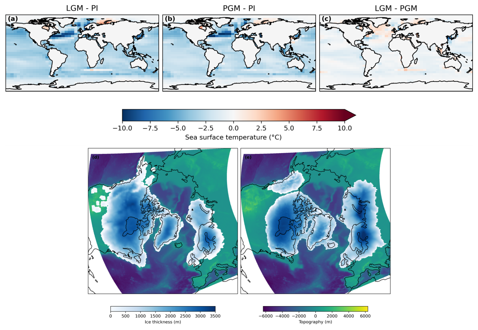
Figure 1 Boundary and initial conditions for the LGM and PGM simulations. Sea surface temperature anomaly from a HadCM3 pre-industrial control run for (a) LGM and (b) PGM; (c) the difference between the prescribed LGM and PGM sea surface temperatures; and initial topography (meters above sea level) and ice thickness in the BISICLES ice sheet model interactive domain for (c) LGM and (d) PGM.

2.3 Experiment design

2.3.1 Boundary and initial conditions

The coupled simulations broadly follow the PMIP4 protocols for the LGM (Kageyama et al., 2017, 2021) and the PGM (Menviel et al., 2019), which prescribe greenhouse gases, orbital parameters and the Antarctic Ice Sheet configuration. Following the method of Patterson et al. (2024), we also prescribe SSTs and Sea ice from HadCM3 simulations of 21 and 140 ka (Fig. 1a–c). A description of the HadCM3 simulations, the justification for this choice of approach, and a discussion on how these SSTs may affect the result is also presented by Patterson et al. (2024).

The interactive ice sheet model domain covers the whole NH, including the North American, Greenland and Eurasian ice sheets. Patterson et al. (2024) showed that the initial ice sheet model conditions used in the glacial maxima simulations overwhelmingly determined the configurations of the final ice sheets due to the ice-albedo feedback, and that the climate at the glacial maxima had an opposite impact on the difference in NAIS ice volume between the LGM and PGM to what was expected. This suggests that the evolution of the climate and the ice sheets leading up to the glacial maximum are important in determining the configurations of the ice sheets at the glacial maximum. We, therefore, chose to initialise the LGM and PGM simulations from the respective ice sheet reconstructions available to ensure realistic ice sheet geometry for each period, accounting for the evolution of the climate and ice sheets prior to the glacial maxima. With this approach, we can examine how the differences in ice geometry and background climate between the 2 time periods affect the sensitivity to the model parameters that control key earth system feedbacks (e.g. ice-albedo feedback, ice-elevation feedback and climate-ice sheet interactions). The LGM orography was initiated from the GLAC-1D reconstruction (Briggs et al., 2014; Ivanovic et al., 2016; Tarasov et al., 2012, Fig. 1d) and the PGM was initiated from a combination of a simulated PGM NAIS by Patterson et al. (2024) and simulated PGM EIS by Pollard et al. (2023) (Fig. 1e) and their corresponding topographies.

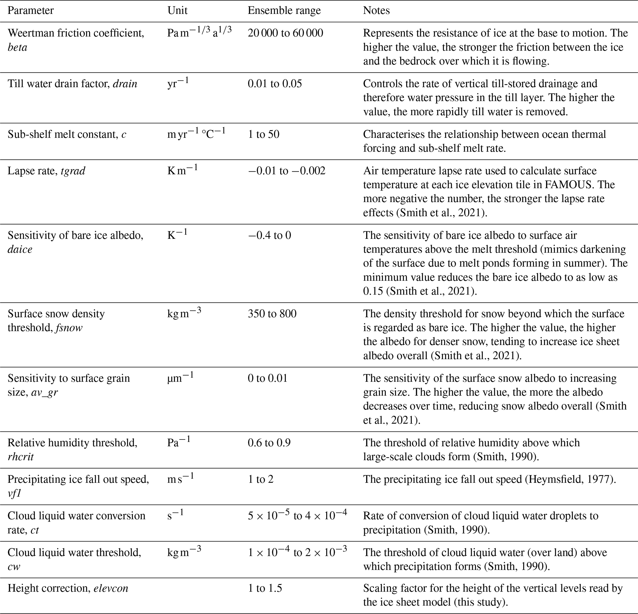
(Smith et al., 2021)(Smith et al., 2021)(Smith et al., 2021)(Smith et al., 2021)(Smith, 1990)(Heymsfield, 1977)(Smith, 1990)(Smith, 1990)

Table 1 Parameters varied in the ensemble and the ranges sampled.

2.3.2 Ensemble design

As well as the initial ice sheet conditions, modelled ice sheet volumes and areas are also sensitive to a number of uncertain parameters related to climate processes, surface mass balance and ice sheet dynamics. To assess this sensitivity, we design an ensemble using maximin Latin Hypercube Sampling (Williamson, 2015; Santner et al., 2003), that consists of 120 combinations of 12 uncertain climate and ice sheet model parameters, varied over a specified range (Table 1). These 120 simulations are each run with the LGM and PGM initial conditions described in Sect. 2.3.1, resulting in 240 total simulations. Each was integrated for 500 climate years (5000 ice sheet years). Since we start from a glacial maximum configuration and spun-up internal temperatures, this is enough time for the ice sheets to (i) reach equilibrium (or close to it), and (ii) give an indication of whether the parameters are producing reasonable ice sheets and form ice streams. Each simulation took around 35 h on 8 cores to complete (∼ 280 core  hours).

The choice and range of parameters is adapted from several previous ensemble studies (Gandy et al., 2023; Gregoire et al., 2011; Patterson et al., 2024; Sherriff-Tadano et al., 2024). We vary 3 uncertain parameters related to ice sheet dynamics in BISICLES; the basal friction coefficient in the power law relation (beta), the till water drain factor (drain), and the sub-shelf melt constant (c). The elevcon parameter controls the magnitude of the height adjustment applied and the remaining parameters control the climatic conditions and ice albedo in the simulations.

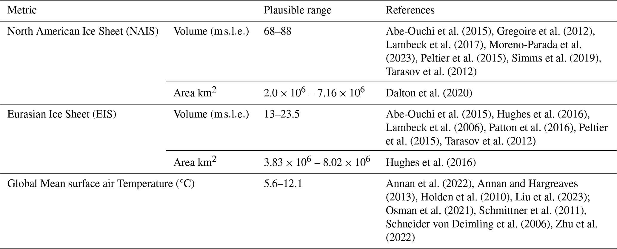
Abe-Ouchi et al. (2015)Gregoire et al. (2012)Lambeck et al. (2017)Moreno-Parada et al. (2023)Peltier et al. (2015)Simms et al. (2019)Tarasov et al. (2012)Dalton et al. (2020)Abe-Ouchi et al. (2015)Hughes et al. (2016)Lambeck et al. (2006)Patton et al. (2016)Peltier et al. (2015)Tarasov et al. (2012)Hughes et al. (2016)Annan et al. (2022)Annan and Hargreaves (2013)Holden et al. (2010)Liu et al. (2023); Osman et al. (2021)Schmittner et al. (2011)Schneider von Deimling et al. (2006)Zhu et al. (2022)

Table 2 The ranges of plausible values for ice sheet volume and extent (in metres global mean sea level equivalent; $\mathrm{m}\mathrm{s}.\mathrm{l}.\mathrm{e}.$), and global mean surface air temperature (°C) used in our implausibility metric, and references to the published work used to derive these ranges.

2.4 Evaluating the ensemble

To evaluate the performance of the LGM ensemble members and find sets of model parameters that produce Not Ruled Out Yet (NROY) ice sheet configurations, we employ an implausibility metric, following a similar approach to Patterson et al. (2024). This allows a robust comparison of model output to empirical evidence and previous modelling studies, taking into account their uncertainties. As in Patterson et al. (2024), the implausibility metric considers constraints on LGM NAIS ice volume and southern ice extent, however, in this study these values have been revised and the metric has been expanded to also include EIS volume and area constraints and Global Mean Air Temperature (GMT). The plausible ranges are derived from studies using palaeo-records of past climate and ice sheets and numerical modelling (Table 2). Since the PGM is poorly constrained in these areas, we are unable to evaluate the performance of the PGM ensemble in the same way. Instead, we opt to select the PGM ensemble members that correspond to the selected LGM members to enable comparison, see whether the same parameter values produce plausible PGM ice sheets based on known configuration differences and allow us to learn more about the PGM without the restriction of uncertain constraints.

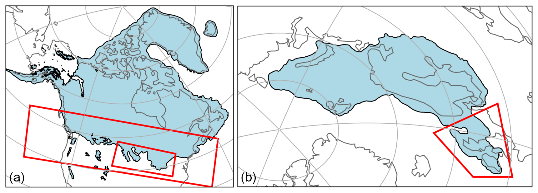
Figure 2 Reconstructions used in the implausibility metric. (a) North American Ice sheet extent from Dalton et al. (2020); the large red box delimits the southern extent footprint used in the implausibility metric; the smaller red box indicates the area of the lobes used to calculate the range of plausible values. (b) Eurasian ice sheet extent from Hughes et al. (2016); the red box indicates the area of the BIIS used to calculate the range of plausible ice areas.

The NAIS area is evaluated based on the southern extent of the ice sheet reconstructed by Dalton et al. (2020), within ± 3 times the area of the ice lobes (Fig. 2a). We set this envelope of uncertainty (based on ice-lobe area) to account for known common model biases, such as over-estimated Alaskan ice, and limitations such as the inability to simulate the dynamic ice lobes (Patterson et al., 2024). Similarly, the plausible range of the EIS is considered to be within ± 3 times the area of the BIIS (Fig. 2b) based on the reconstruction from (Hughes et al., 2016), since none of our simulations maintain ice over this area (see Sect. 3.1) and we do not want to compensate for/hide this limitation by over-estimating ice elsewhere. The GMT range is determined from different estimated levels of LGM cooling, and their uncertainties, relative to a pre-industrial GMT of 13.7 ± 0.1 °C (1880–1900; NOAA National Centers for Environmental Information, 2023; Sherriff-Tadano et al., 2024).

2.5 Gaussian process emulation and Sobol sensitivity analysis

To determine which of the model parameters had the most influence on the uncertainty in modelled ice sheet configurations, and whether this differed for each of the NH ice sheets and each glacial maxima, we perform a Sobol Sensitivity Analysis (Saltelli, 2002; Sobol', 2001) on 4 diagnostics for each ensemble; NAIS ice volume, NAIS southern area, EIS ice volume and EIS area. This produces a first order sensitivity index which measures the contribution to the output variance by each model parameter alone; a second order index which measures the contribution from interactions between two parameters and; a total order index which is the contribution by a model parameter as a result of its first order sensitivity and all higher order interactions. An index value of 0.05 is often used as the threshold above which a parameter is considered to have an important influence on the output variance (Zhang et al., 2015).

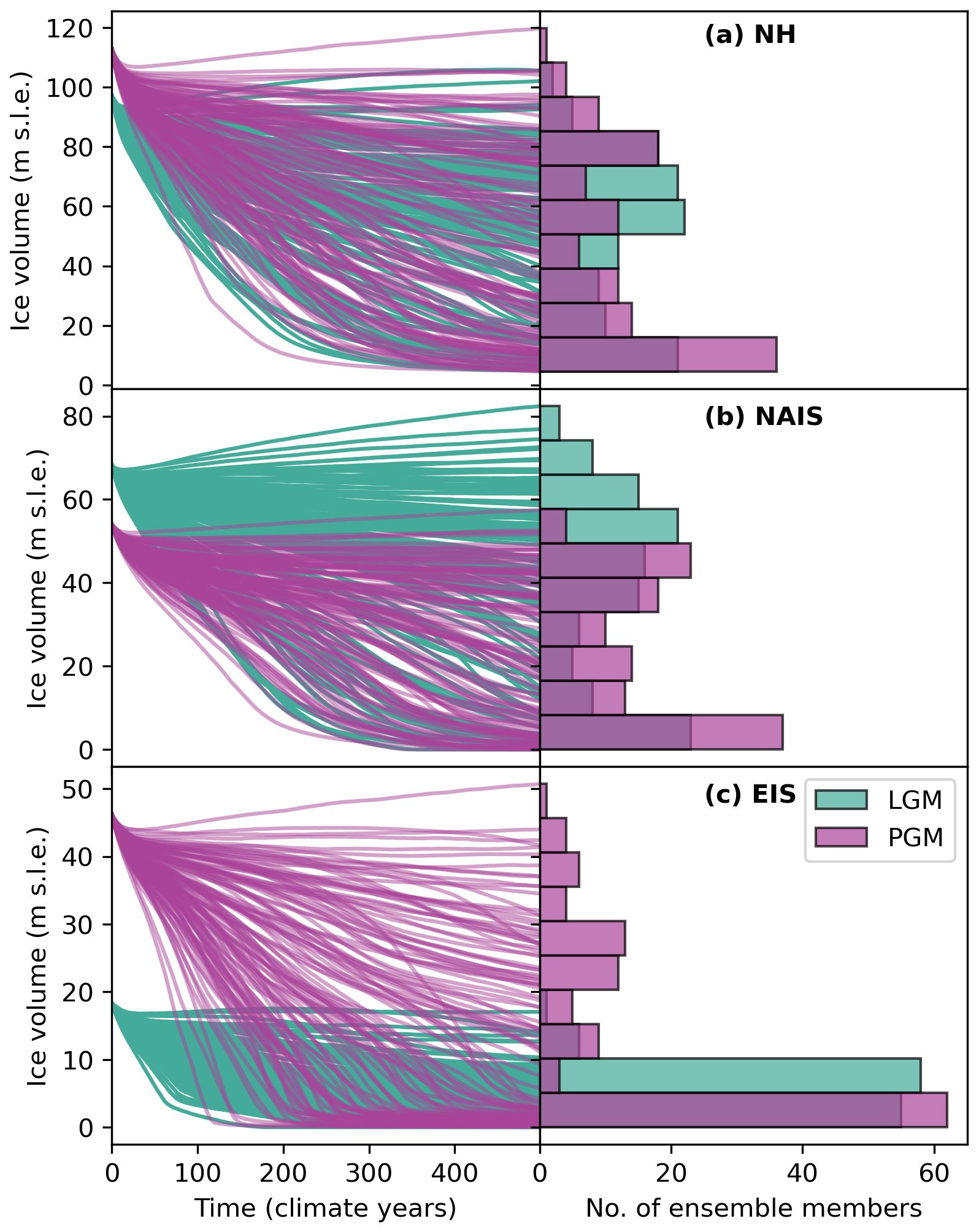
Figure 3 Time series of ice volume over the 500 climate years (5000 ice sheet years) of simulation for each ensemble member (left hand panels) and histograms of the distribution of final ice volumes across the ensembles (right hand panels) for the LGM and PGM (a) Northern Hemisphere; (b)yNorth American ice sheet and (c) Eurasian ice sheet.

The Sobol analysis requires a uniform sample of thousands of model inputs, for example, generated following Saltelli's extension of the Sobol sequence, which are outside of our initial parameter sample. This would therefore require additional evaluations of the model, which would require significant additional computational resources. To this end, we train independent Gaussian Process (GP) emulators (Kennedy and O'Hagan, 2001; Oakley and O'Hagan, 2004) on each of the 4 diagnostics from the two 120 member ensembles. These emulators are then employed to evaluate the additional parameter sets generated by the Sobol sequence. Using this sequence and the emulators, we are able to generate and evaluate more than 200 000 samples in only a few minutes, a number which would have been computationally intractable using FAMOUS-BISICLES directly. Since we use a complex model with a large number of uncertain parameters, a sample of this size is necessary in order to increase the reliability of the Sobol analysis.

To evaluate the performance of our emulators and ensure their predicted output is sensible compared to the modelled output, we perform a Leave-One-Out Cross-Validation (LOOCV) on each emulator (Bastos and O'Hagan, 2009; Rougier et al., 2009). In general, leave-k-out cross-validation involves splitting the dataset of input parameters and output diagnostics into separate training sets and testing sets. An emulator is fitted to the training set and then fed the input parameters from the test set to evaluate. The values it then predicts is then compared to the actual modelled values. In the case of the LOOCV, all but 1 set of inputs and outputs are used as the training set and the emulator is used to predict the output left out. This process is then repeated for each of the 120 model outputs. We found that, compared to the modelled outputs, 7 of the ensemble input parameter sets consistently produced poor predictions for 4 or more of the 8 diagnostics. Therefore, to improve the quality of the emulator fit, we removed these 7 inputs, re-trained the emulators, and once again performed the LOOCV. The predicted values (and their 95 % credible intervals) compared to the modelled values for each emulator are shown in Appendix D (Fig. 1). Overall, between 84 %–93 % of the predicted intervals contain the true model output, which we determine is enough for the purposes of the Sobol analysis.

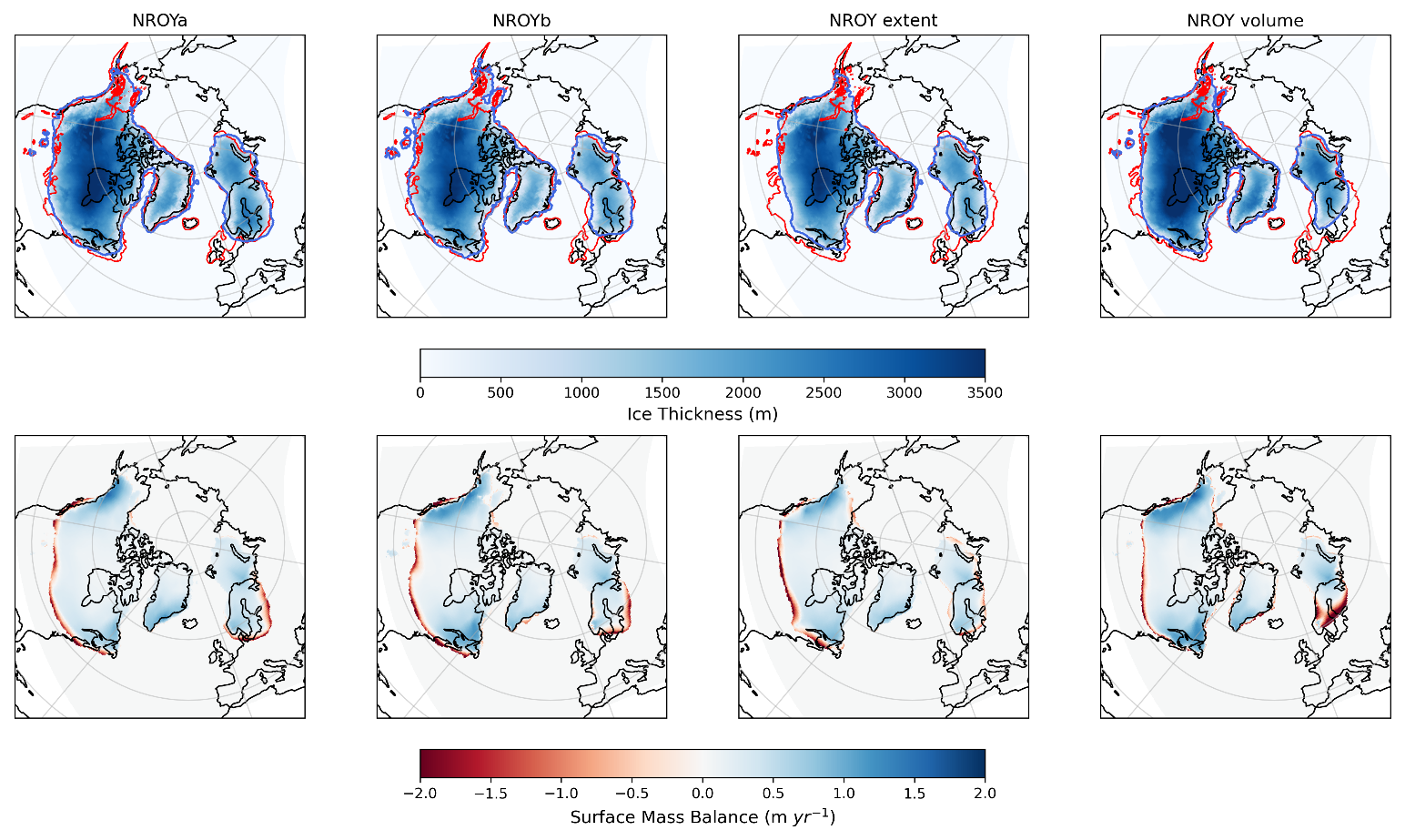
Figure 4 Final ice thickness and surface mass balance for the 4 NROY LGM simulations. The red contours indicate the reconstructed LGM ice sheet extents of Dalton et al. (2020) and Hughes et al. (2016) and the blue contours indicate the extent of the modelled ice sheets displayed in the figure.

3 Results

3.1 Ensemble

After running the ensembles of simulations for the LGM and PGM, we obtain 2 sets of 120 simulations with a wide spread of NH ice sheet configurations (Fig. 3). The ensemble mean volume of the NAIS at the LGM is 37.6 $\mathrm{m}\mathrm{s}.\mathrm{l}.\mathrm{e}.$, with a smaller mean at the PGM of 22.8 $\mathrm{m}\mathrm{s}.\mathrm{l}.\mathrm{e}.$ In contrast, the LGM has a smaller mean EIS volume of 5.39 $\mathrm{m}\mathrm{s}.\mathrm{l}.\mathrm{e}.$ compared to 12.6 $\mathrm{m}\mathrm{s}.\mathrm{l}.\mathrm{e}.$ at the PGM. Both ensembles have a similar mean Greenland ice sheet volume of ∼ 7 $\mathrm{m}\mathrm{s}.\mathrm{l}.\mathrm{e}.$ The evolution and distributions of ice volume across the ensembles shown in Fig. 3 reveals that ice sheets collapse in a significant proportion of simulations due to an unsuitable combination of parameter values, but that many simulations sustain the initial ice volume, and a few grow.

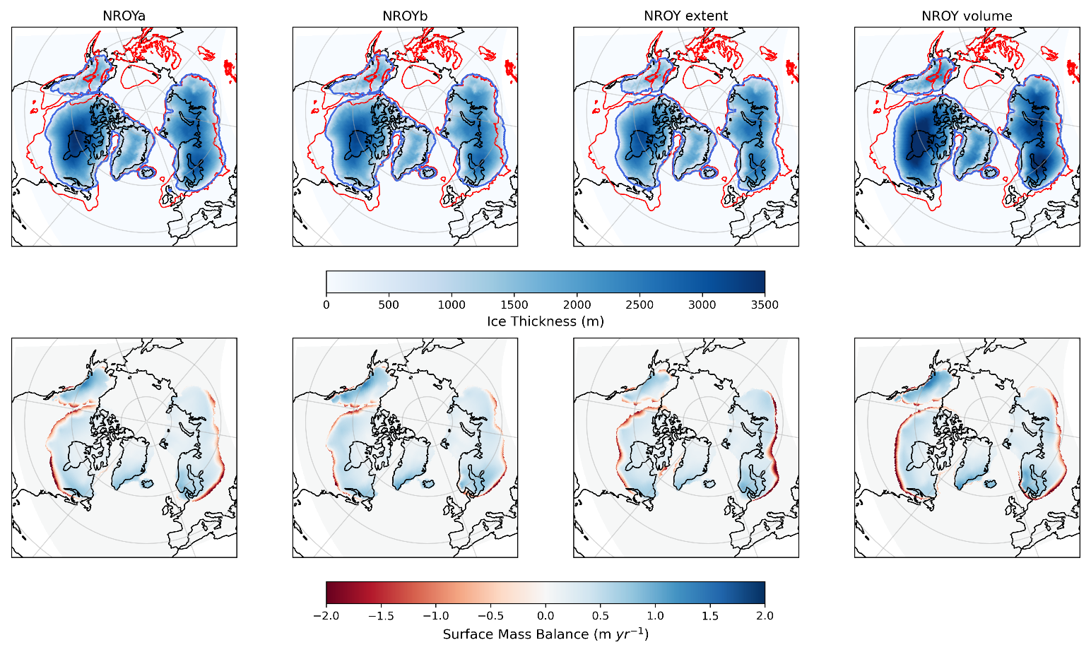
Figure 5 Final ice thickness and surface mass balance for the 4 NROY PGM simulations. The red contours indicate the reconstructed MIS 6 ice sheet extents of Batchelor et al. (2019) and the blue contours indicate the extent of the modelled ice sheets displayed in the figure.

Table 3 Ice sheet volumes and extents at the end of the 5000 ice sheet years for the 2 NROY LGM simulations and the corresponding PGM simulations.

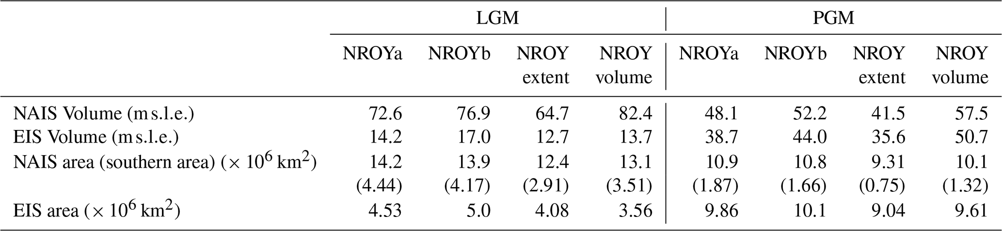
We apply the implausibility metric described in Sect. 2.4 to the ensemble of LGM simulations to identify sets of model parameters that produce plausible ice sheets. All ensemble members have a global mean surface air temperature within the plausible range (6.3–9.2 °C at the LGM and 7.1–10.1 °C at the PGM) due to the prescribed SSTs. 2 LGM simulations fit all 4 of our implausibility criteria for the volume and extent of both the NAIS and EIS, we label these NROYa and NROYb. The proportion of NROYs in an ensemble is highly dependent on the subjective choice of number and ranges of parameter values sampled. Previous work with FAMOUS-ice (Gandy et al., 2023; Patterson et al., 2024; Sherriff-Tadano et al., 2024) has shown that finding combinations of parameter values that produce realistic ice extent during glacial times is challenging, due to strong albedo-surface mass balance feedbacks. Thus, finding 2 parameter combinations that produce plausible results for both time periods and both ice sheets is a good outcome. Additional simulations from the NROY parameter space could be found by iterating this process and using emulators within the implausibility measures to efficiently identify such parameter combinations given the first ensemble, as was done in Patterson et al. (2024). This is computationally expensive and was not required for our purposes. Nevertheless, we apply the extent and volume constraints separately to explore additional plausible ice sheet configurations, especially since the volume constraint is still very uncertain and our minimum volume for the NAIS is less lenient than limits that have been used previously (e.g. Gandy et al., 2023; Sherriff-Tadano et al., 2024). This results in the selection of 2 more ensemble members; 1 that meets only the ice extent criteria (labelled as NROY extent) and 1 that meets only the ice volume criteria (labelled as NROY volume). All four NROY simulations are shown in Fig. 4, with the corresponding 4 PGM simulations presented in Fig. 5. The time series of ice volume, surface mass balance and sub-shelf melt plus calving rate for these simulations are provided in Appendix E. The final volumes and extents of the NROY simulations are outlined in Table 3. A full comparison of the simulations against reconstructions of ice extent and other modelling studies is presented in Sect. 4.1.

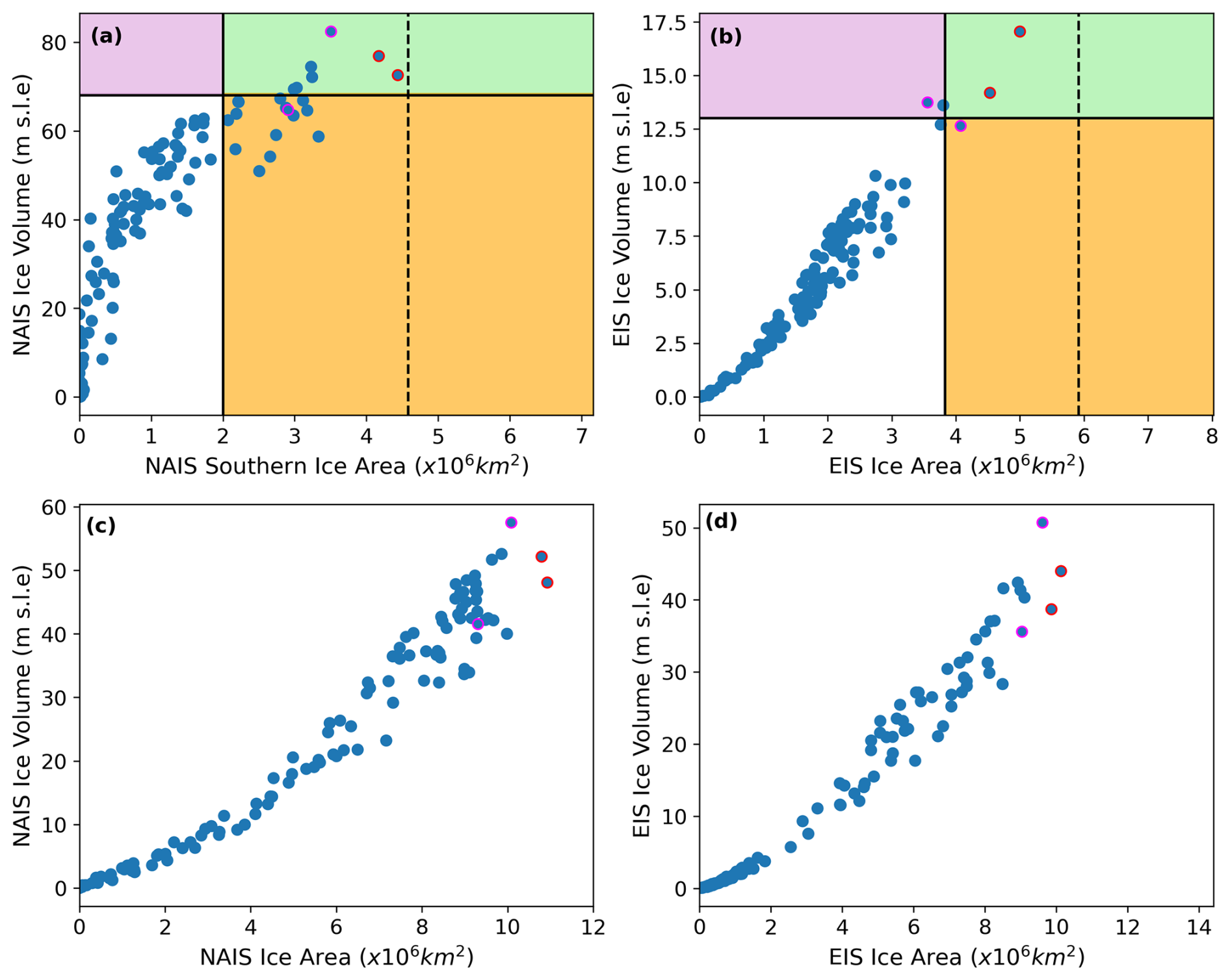
Figure 6 Results from the full ensembles of simulations showing (a) LGM North American ice sheet southern area versus volume and (b) LGM Eurasian ice sheet area versus volume. The solid lines show the minimum values used in the implausibility metric for area and extent and the dotted line shows the actual extent of the ice sheet reconstructions. Simulations that fall within the green box satisfy area and volume constraints for each individual ice sheet, the orange box indicates they satisfy the area constraints only and purple only the volume constraints. The points outlined in red are the 2 NROY simulations (i.e. fall into the green box for both ice sheets) and the points outlined in pink are the additional NROY extent and NROY volume simulations. Panels (c) and (d) show the equivalent results for the PGM ensembles without the constraints.

The parameter values used in the 2 NROYa and NROYb simulations are in a similar region of the parameter space for all parameters except tgrad (lapse rate) and drain (till water drainage rate), suggesting the ice sheets are fairly insensitive to these 2 parameters (Fig. S1 in the Supplement). Interestingly, there are 5 simulations that produce only a plausible LGM NAIS but do not meet constraints for the EIS (Fig. 6a and b) . Furthermore, as we have already seen, there are also simulations that produce plausible ice sheet extents but fall short on the volume and vice versa. Many of these simulations are situated in different areas of the parameters space than the 2 NROY simulations for most of the parameters (Fig. S1 in the Supplement). Figure 6c and d shows that the NROYa and NROYb parameter sets also produce the largest PGM ice sheet extents in the ensemble but there are additional simulations that produce an EIS of similar or larger volume, which was not the case for the LGM. These results all suggest that both ice sheets and both time periods display different sensitivities to model parameters.

3.2 Parameter sensitivities

We used Gaussian Process emulation and Sobol Sensitivity analysis (Sect. 2.5) to quantify the sensitivity of ice extent and volume to the model parameters we varied. Given emulator uncertainties, we focus on the largest values and differences between the Sobol indices. We encourage the reader not to over-interpret the relative importance of the less significant parameters.

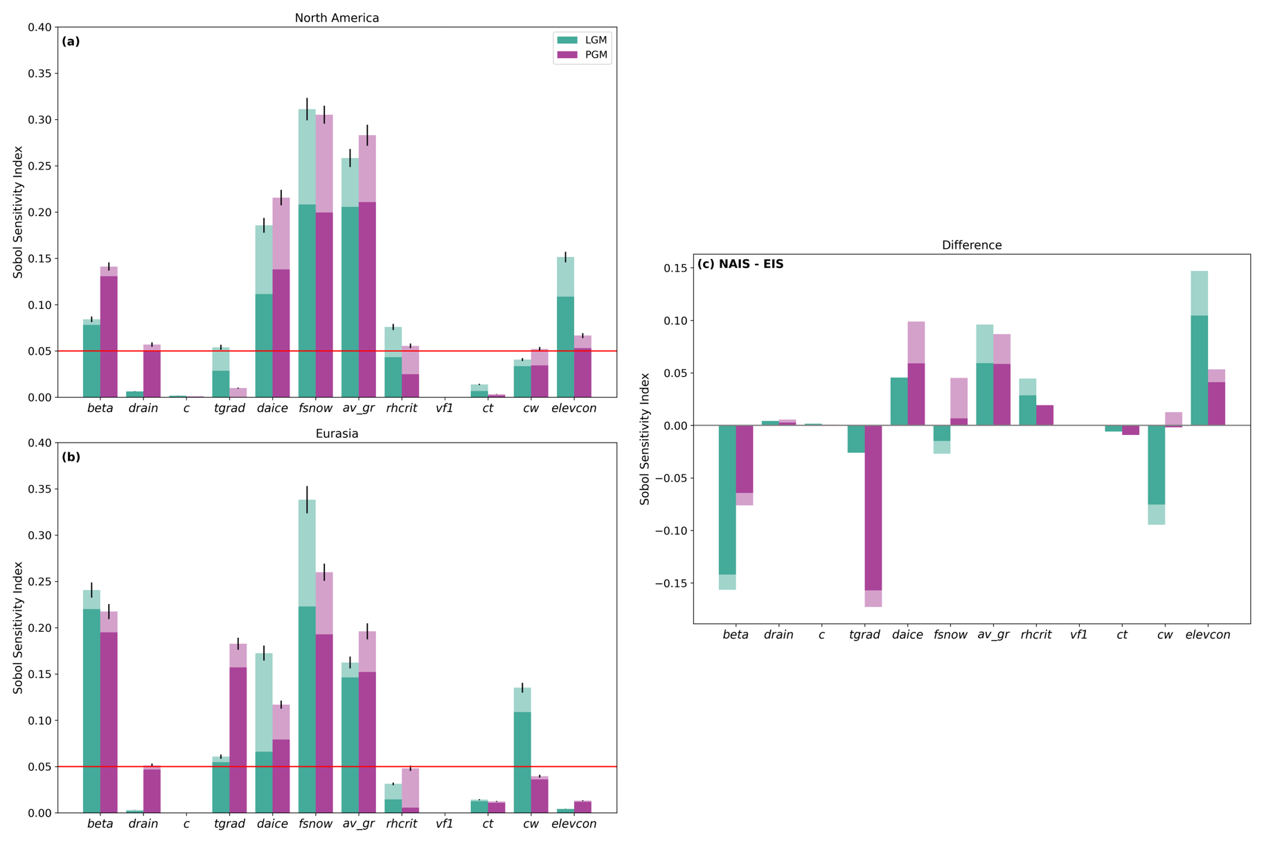
Figure 7 The Sobol sensitivity index of the ice volume for each parameter for (a) the North American Ice Sheet and (b) the Eurasian Ice Sheet. (c) The difference in sensitivity indices between the North American and Eurasian ice sheets. The darker colour represents the first order index and the lighter colour the second order index (together showing the total sensitivity). The variance of the Sobol indices plus the mean emulator variance is indicated by the black error bars. The red line indicates the index value of 0.05, above which the sensitivity is significant.

Figure 7 shows the first and second order sensitivity indices for the NAIS and EIS volumes during the LGM and PGM. The ice sheets were relatively insensitive to the parameters vf1 (precipitating ice fall out speed), drain (till water drainage rate), ct (cloud liquid water conversion rate), rhcrit (relative humidity threshold) and c (sub-shelf melt constant).

The most influential parameters are fsnow (surface snow density threshold) and av_gr (sensitivity to grain size), which control the albedo of the ice sheet, with larger values of fsnow and smaller values of av_gr leading to larger ice sheets. Daice (bare ice albedo sensitivity) also played a role, especially for the NAIS, though its effect was secondary when fsnow and av_gr already produced high albedo (Fig. F1). These 3 albedo parameters also showed strong interactions with each other and other parameters. Our Sobol analysis not only confirms the importance of albedo parameters, consistent with previous studies (Gandy et al., 2023; Patterson et al., 2024; Sherriff-Tadano et al., 2024), but also quantifies the influence of other parameters, particularly for the EIS. For the EIS, the other important parameters are beta (Weertman friction coefficient), cw (cloud liquid water threshold) at the LGM, and tgrad (lapse rate), especially for the PGM. The NAIS is also sensitive to new parameters introduced in this study that were not tested in Gandy et al. (2023) or Patterson et al. (2024), including beta, and elevcon (height correction; which the LGM volume is sensitive to). We discuss the reasons why parameters are more or less important for different ice sheets and time periods in Sect. 4.2

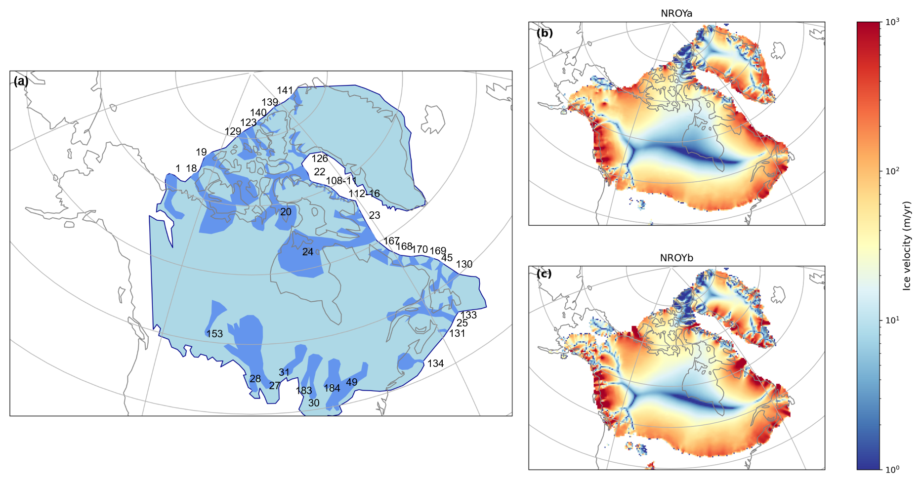
Figure 8 (a) Empirical reconstruction of the active LGM Laurentide ice sheet ice streams (adapted from Margold et al. (2018), and (b) NROYa and (c) NROYb ice velocities at the end of the 5000 year simulations.

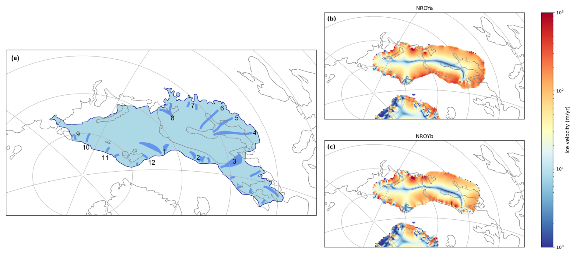
Figure 9 (a) Empirical reconstruction of the active LGM Eurasian ice sheet ice streams (adapted from Patton et al. (2017), and (b) NROYa and (c) NROYb ice velocities at the end of the 5000 year simulations.

3.3 Ice dynamics

By performing an internal temperature spin-up and sensitivity tests (Sect. 2.2 and Appendices B and C), we have improved ice streaming in our simulations compared with FAMOUS-BISICLES simulations of the NAIS (Sherriff-Tadano et al., 2024). Ice stream velocity in the NROY simulations ranges from a few hundred m yr⁻¹ to 5000 m yr⁻¹, in agreement with present day observations of Antarctica and Greenland (Joughin et al., 2010; Rignot et al., 2011). We assess to what extent the modelled ice streams in the simulations match empirical reconstructions by performing a qualitative comparison of NROYa and NROYb to LGM reconstructions of the Laurentide (Fig. 8a; Margold et al., 2018) and Eurasian ice streams (Fig. 9a; Patton et al., 2017).

For the Laurentide Ice Sheet, the locations of many of the ice streams show good agreement, particularly in NROYb (Fig. 8). This includes; (1) Mackenzie Trough, (18) Amundsen Gulf, (129) Prince Gustaf Adolf Sea, (123) Massey Sound, (126) Smith Sound/Nares Strait, (22) Lancaster Sound, (23) Cumberland Sound, (24) Hudson Strait, (45) Notre Dame Channel, (133) Placentia Bay-Halibut Channel, (25) Laurentian Channel, (131) The Gully and (134) Northeast Channel IS (see labels in Margold et al., 2018). There are also areas of general streaming where many smaller ice streams are found (numbers 108–116 and 167–170). One major ice stream that is not very active in these simulations is (19) M'Clure Strait and there is a poor representation of ice streaming along the southern margin of the Laurentide Ice Sheet.

The Eurasian Ice Sheet does not have as defined areas of ice streaming, nevertheless, some of the major ice stream features can be picked out (Fig. 9). There is some streaming activity in the location of 1 of the major ice streams, (1) Bjornoyrenna ice stream, and (10) Svyataya Anna ice stream is relatively well represented. Some of the smaller ice streams are also modelled including; (2) Mid Norwegian, (8), (9), (11) and (12). However, other major and minor ice streams are not active in these simulations; (3) Norwegian Channel, (4) and (5) Baltic Sea, (6) Gulf of Bothnia and (7) (see labels in van Aalderen et al., 2024 and Stokes and Clark, 2001). In addition, since the BIIS is not present, neither are the ice streams in this region. Interestingly, there are active areas of ice streaming to the south of the Barents Sea that are not present in the reconstruction. This could be due to the formation of a pro-glacial lake in this region allowing the formation of ice shelves which have zero basal friction and therefore increase ice velocity (Sutherland et al., 2020).

There are no comparable reconstructions of PGM ice streaming due to difficulties in dating and the erasure of glaciological evidence following the Last Glacial advance. However, due to the extent and topographic constraints on ice streaming, it is likely that ice stream locations were similar across the marine margins of the ice sheets (Pollard et al., 2023). The simulated PGM NAIS velocity behaves similarly to the LGM but there is a lack of (1) Mackenzie Trough and a less pronounced (18) Amundsen Gulf as a result of the different configurations of the ice sheets in this area (i.e. the location of the ice-free corridor between the Laurentide and Cordilleran ice sheets). However, there is more evidence of (19) M'Clure Strait in NROYa and more activity on the southern Laurentide margin (Fig. G1). The PGM EIS velocity shows a more defined (3) Norwegian Channel ice stream and NROYb has a better representation of (10) Svyataya Anna, (11) and (1) Bjornoyrenna ice stream than the LGM. There is still no streaming in the Baltic Sea but the PGM also shows activity in the South Barents Sea. There is also additional ice streaming in the Northeast where the PGM ice sheet extend further than at the LGM (Fig. G2).

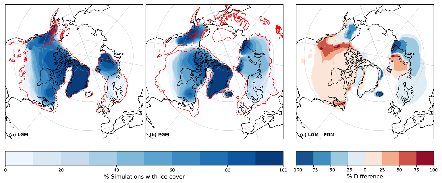
Figure 10 Percentage of ensemble members that had ice in each grid cell of the domain for (a) the LGM (with the extents of Dalton et al. (2020) and Hughes et al. (2016) in red); (b) the PGM (with Batchelor et al. (2019) extent in red); and (c) the difference between the LGM and PGM ensembles.

4 Discussion

4.1 Comparison to reconstructions

Across the LGM ensemble, we simulate a larger North American ice sheet and a smaller Eurasian ice sheet than across the PGM ensemble. The NAIS also maintains the connection between the Cordilleran and Laurentide ice sheets in a significant proportion (70 %–80 %) of the LGM ensemble members (Fig. 10a), while the corridor between the 2 ice sheets remains free in all the PGM simulations (Fig. 10b). These different configurations are consistent with ice sheet reconstructions (Dalton et al., 2020; Batchelor et al., 2019) and are primarily caused by the differences in initial conditions as demonstrated by Patterson et al. (2024).

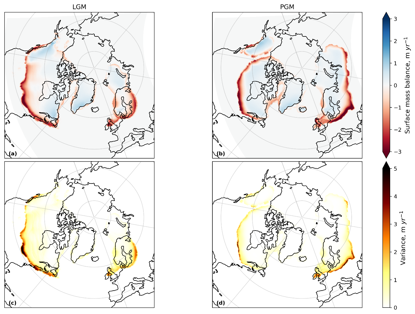
Figure 11 Ensemble mean surface mass balance and variance at ice sheet year 200 for (a) and (c) the LGM and (b) and (d) the PGM.

However, some areas are systematically deglaciated in the ensembles of simulations producing a poor match to the reconstructed extents. In particular, all simulations lack a British-Irish Ice Sheet (BIIS), and most underestimate the extent over Scandinavia and the South-Eastern Laurentide (North American). This is due to large negative SMB values over these regions (Fig. 11) causing rapid deglaciation, with the BIIS disappearing in 600 ice sheet years or less. This is a similar result to Bradley et al. (2024) who used the CESM2.1 model to simulate the SMB across the LGM ice sheets. Their simulations showed large ablation areas across the BIIS, the southern margin of Scandinavia and the southern, Pacific and Atlantic margins of the NAIS, but low melt rates across the Barents–Kara Ice Sheet and Greenland. Whilst they did not use a dynamical ice sheet model, they concluded that if this SMB pattern was applied to one, it would very likely drive rapid retreat of the southern margins of both ice sheets. By testing 120 combinations of parameter values, our study is able to find model configurations with weaker ablation across some of these regions, reducing some of the SMB biases of Bradley et al. (2024).

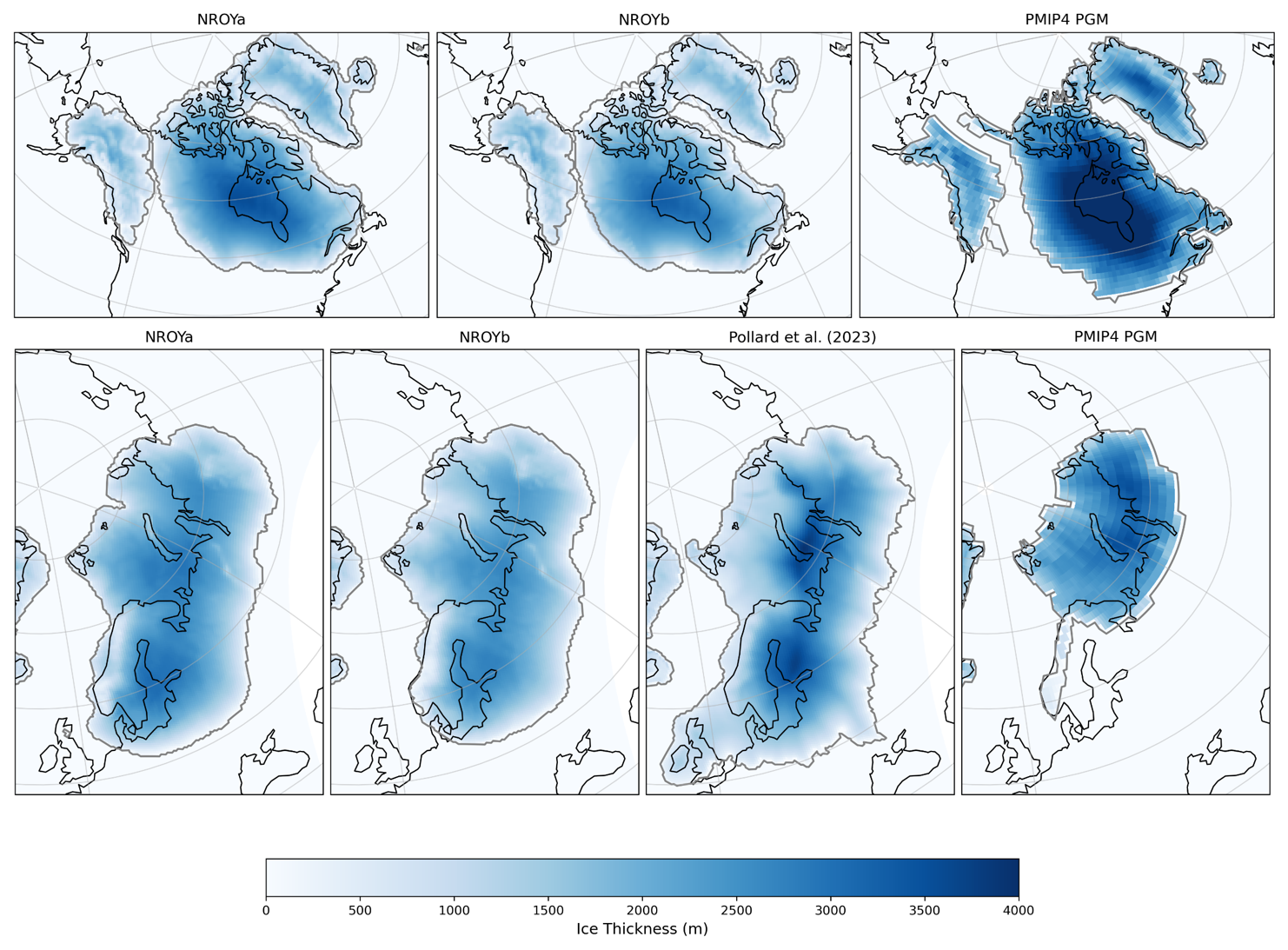
Figure 12 Comparison of the 2 NROY PGM simulations to other model reconstructions (Abe-Ouchi et al., 2013; Pollard et al., 2023)

The underestimation of ice extent in particular regions, compared to reconstructions, could reflect the asynchronous timing of the local maxima of the NH ice sheets since, for example, there is evidence that much of the NAIS reached its maximum extent at ∼ 25 ka (Dalton et al., 2022, 2023) and the BIIS reached it maximum at ∼ 25–23 ka before starting its retreat at ∼ 22 ka due to a warming trend caused by a change in orbital parameters between 26–21 ka (Clark et al., 2022; Hughes et al., 2016). However, these reconstructions of the NAIS and BIIS still suggest there was extensive ice over these regions at 21 ka even if not at their maxima. In addition, Bradley et al. (2024) also performed a simulation using boundary conditions for 26 ka and obtained a similar result to 21 ka. They therefore concluded that the too negative SMBs are likely a result of biases in the simulated climate or ice sheet reconstruction, a highly non-equilibrated climate and ice sheet at the LGM, and/or the need to retune the model for LGM climate conditions (as also shown to be necessary by Gandy et al., 2023). Indeed, many other numerical modelling studies have also found it difficult to maintain extensive ice in these regions using a range of different models, boundary conditions and model parameters (van Aalderen et al., 2023; Quiquet et al., 2021; Scherrenberg et al., 2023; Sherriff-Tadano et al., 2024; Ziemen et al., 2014; Zweck and Huybrechts, 2005).

Overall, the LGM NROY simulations show a good match to the reconstructed extents of the LGM ice sheets and the equivalent PGM simulations display a smaller NAIS and larger EIS in line with empirical evidence and previous studies (Figs. 4 and 5). Whilst the PGM simulations show a smaller NAIS than the extent of Batchelor et al. (2019), this latter reconstruction represents the maximum MIS 6 extent (190–132 ka) and therefore is likely larger than the 140 ka ice sheet would have been, particularly for the NAIS. These 4 NROY model simulations suggest the NAIS was ∼ 25 $\mathrm{m}\mathrm{s}.\mathrm{l}.\mathrm{e}.$ smaller at the PGM compared to the LGM, and the EIS ∼ 24–27 $\mathrm{m}\mathrm{s}.\mathrm{l}.\mathrm{e}.$ larger. There are very few existing reconstructions of the PGM ice sheets and none produced using a coupled climate-ice sheet model. Our simulations perform well in comparison to these reconstructions (Fig. 12) . For example, compared to the reconstruction of Pollard et al. (2023), our Eurasian ice sheet is more physically consistent with climate and ice sheet dynamics but is also more in line with empirical reconstruction of ice extent (e.g. Batchelor et al., 2019) compared to the dynamic ice sheet model reconstruction used in the PMIP4 protocol (Abe-Ouchi et al., 2013; Menviel et al., 2019), which is missing most of the Fennoscandian ice sheet (Fig. 12). Thus, our NROY simulations provide new improved reconstructions of the PGM Northern Hemisphere ice sheets for use as inputs for climate, ice sheets and sea level models.

All NROY simulations lack a BIIS suggesting this feature is due to our modelling setup rather than parameter uncertainty. The BRITICE-CHRONO comprehensive reconstruction of the BIIS deglaciation revealed that the ice sheet reached its maximum extent around 26 ka (or before in some sectors) and had initiated a rapid collapse at 22 ka which saw most of the ice sheet disintegrate by 16 ka (Clark et al., 2022). We can infer that the BIIS was at disequilibrium with the 21 ka climate and had significantly negative surface mass balance leading to the collapse of the ice sheet within ∼ 5000 years. The full deglaciation of the BIIS during our 5000 year long equilibrium simulations under 21 ka forcing is thus in agreement with the BRITICE-CHRONO reconstruction. Transient coupled climate-ice sheet simulations would be required to simulate the rapid growth and retreat of the BIIS around the LGM.

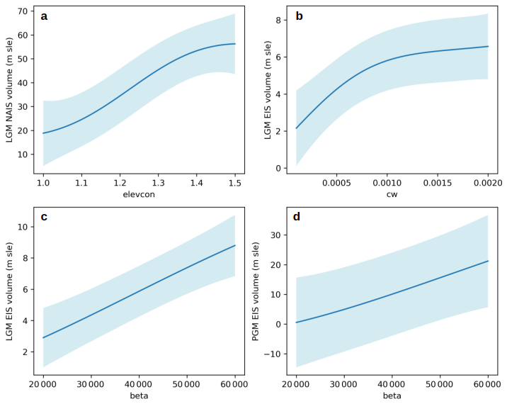
Figure 13 The relationship between emulated mean ice sheet volumes and (a) elevcon, (b) cw, (c) and (d) beta. The 95th percentiles are shown by the blue shaded region.

Due to high rates of sub-shelf melt (∼ 60–75 m yr⁻¹), the NROY simulations also lack ice shelves by the end of the 5000 ice sheet years, which could also have contributed to the underestimation of the eastern margin of the NAIS and the deglaciation of the BIIS (Scherrenberg et al., 2023). However, there are not many constraints on the extent of ice shelves during the LGM or PGM since they leave few glaciological traces behind. There is some evidence that a large, thick ice shelf extended into the Arctic Ocean during the MIS 6 glaciation (Jakobsson et al., 2016; Svendsen et al., 2004) and during the last glaciation a thick ice shelf may have covered Baffin Bay (Couette et al., 2022). Similarly, the rate of sub-shelf melt is poorly constrained during past periods, however, since some studies have shown ocean driven melt to be important for the evolution of the marine based sectors of the NH ice sheets (Alvarez-Solas et al., 2019; Clark et al., 2020; Petrini et al., 2020), it may be useful to implement a more complex parameterisation or perform some additional sensitivity tests to explore this process further in future studies.

Despite difficulties in the past in obtaining a sufficient southern extent of the LGM NAIS in lower resolution models (Gandy et al., 2023; Sherriff-Tadano et al., 2024; Ziemen et al., 2014), the NROYa and NROYb simulations do a relatively good job, with the southern ice sheet area only falling short of the Dalton et al. (2020) reconstruction by 3 % and 9 %, respectively. The 2 additional NROY simulations are less close to the reconstructed extent, however, and all 4 still fail to capture the ice lobe structures. This is because they are formed by extensions of terrestrial ice streams as a result of complex ice dynamics and subglacial processes (Jennings, 2006; Margold et al., 2018). They are also highly asynchronous, dynamic features resulting in their glacial maximum limits being very uncertain (Dalton et al., 2020; Margold et al., 2018). Therefore, it is not surprising that a relatively low resolution climate and ice sheet model with a simple representation of subglacial processes is unable to resolve such features (Gandy et al., 2019; Zweck and Huybrechts, 2005).

4.2 Influence of parameters on ice sheet configurations

To help isolate the effect of individual parameters on ice sheet volume, and help explain the sensitivities discussed in Sect. 3.2, we use emulation to vary 1 parameter at a time while holding the others at their midpoints (Fig. 13).

.

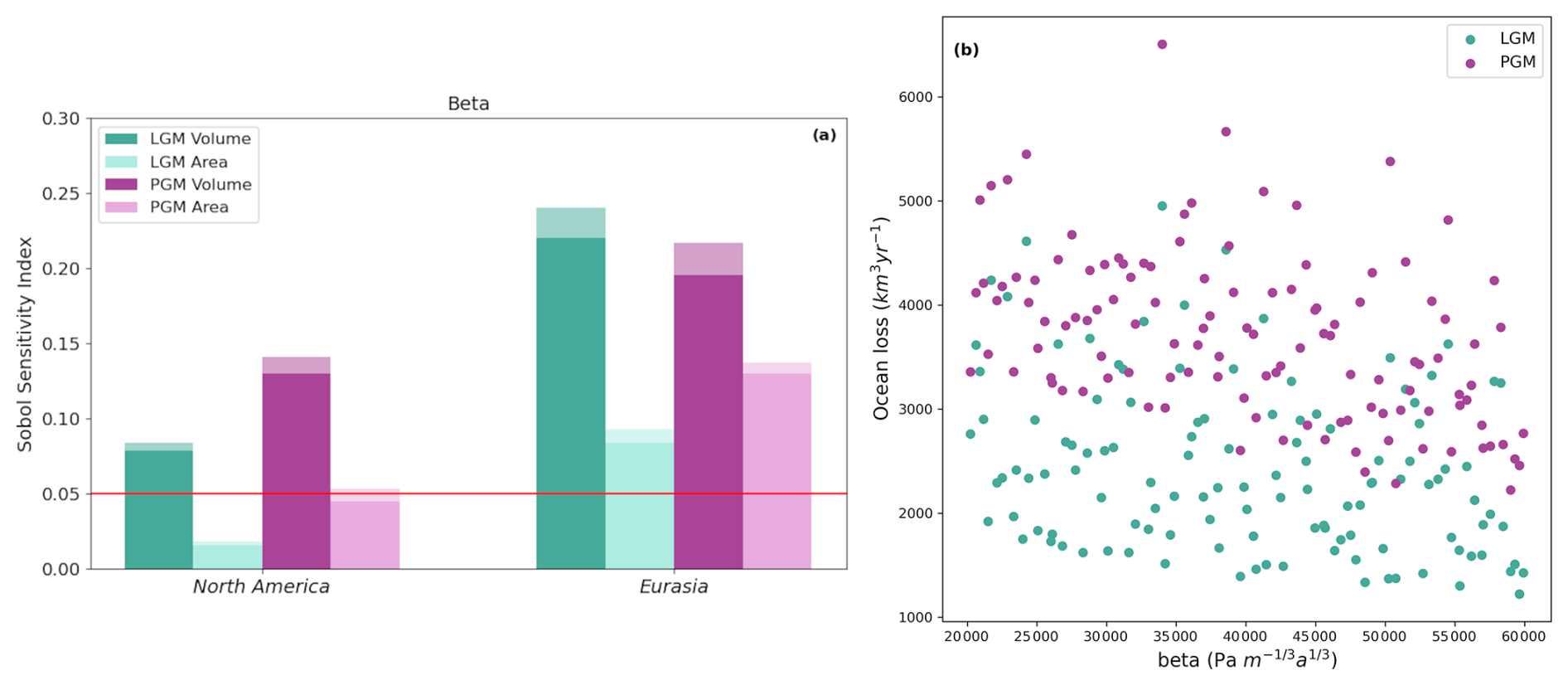
Figure 14 (a) Sobol Sensitivity Indices for the ice volume and extent at the LGM and PGM for the parameter beta and (b) LGM and PGM calving plus sub-shelf melt flux averaged over the whole duration of the simulations versus the value of beta

The low sensitivity of ice sheet size to c (sub-shelf melt constant) is expected, as ice shelves were lost early in the simulations due to high sub-shelf melt or ablation from other climate parameters. We expect that the sub-shelf melt constant c would have much more influence in the context of deglaciations than in the equilibrium simulations we ran here. Similarly, drain (till water drainage rate) is more important for the characteristics of ice flow than for ice volume and extent.

The sensitivity of the LGM NAIS to elevcon could be related to the size of the ice sheets since it affects higher ice elevations more. Indeed we find the value of the elevcon Sobol index is proportional to the average thickness of each ice sheet. The fact that a larger value of elevcon leads to a larger NAIS (Fig. 13a) but does not impact the size of the EIS could explain why the ensemble produced more plausible North American ice sheets at the LGM but did not perform as well for the Eurasian ice sheet (Fig. 6).

The sensitivity of LGM EIS to cw (cloud liquid water threshold) suggests that the EIS is more sensitive to differences in precipitation than the NAIS. This likely reflects differences in the climatic regimes of both ice sheets imposed by their geographical locations. Indeed the EIS is subject to a more maritime climate than the NAIS with higher precipitation rates and cloudiness sensitive to cw. Interestingly at the PGM, the EIS is less sensitive to this parameter, likely because its larger size puts its southern margins in a more continental climatic regime less sensitive to precipitation rates or cloud cover. Cw has a positive correlation with EIS volume up to a value of around 0.0012 kg m⁻³ (Fig. 13b) above which volume plateaus. This could be because lower values of cw cause increased precipitation due to decreasing the threshold of cloud liquid water above which precipitation forms. This leads to higher summer rainfall contributing to the surface melting through the heat flux from rain to ice. The LGM EIS is particularly susceptible to this effect due to its smaller size. Precipitation is not downscaled onto elevation tiles in the coupling, rather the coarse atmospheric output is applied to the ice sheet model which leads to rainfall being spread across relatively large areas of the ice sheet, therefore affecting a large proportion of the LGM EIS (Smith et al., 2021). Therefore, the use of a higher resolution atmospheric model or an improvement to the coupling scheme may reduce the sensitivity to this parameter (Dong and Valdes, 2000; van Kampenhout et al., 2019; Lofverstrom and Liakka, 2018). Another reason the LGM EIS is positively correlated with cw could be related to the change in liquid cloud cover and its effect on the energy balance. The increased precipitation leads to a decrease in the fraction of cloud cover which would allow a higher receipt of incoming shortwave radiation, thus increasing the surface melt. However, the downwelling longwave radiation may also be decreased which would have the opposite effect, decreasing the absorbed energy. Since the accumulation zone usually has a high albedo, reflecting much of the incoming solar radiation, the SMB of this area is mostly controlled by changes in the longwave fluxes. In contrast, the low albedo ablation zone is largely impacted by the shortwave radiation budget in the summer melt season. This latter process has been found to be dominant in studies of the Greenland Ice Sheet, with reduced cloudiness contributing to its mass loss and increasing its sensitivity to warming (Hofer et al., 2017; Izeboud et al., 2020; Mostue et al., 2024; Ryan et al., 2022). Again, due to its smaller size, a large proportion of the LGM EIS is under ablation (54 % compared to around 35 % for the other ice sheets in Fig. 11), potentially explaining why it is so sensitive to changes in cloud cover.

PGM EIS is much more sensitive to the value of tgrad than the other ice sheets. More negative values of tgrad cause a stronger temperature-elevation feedback, resulting in warmer temperatures at lower elevations. This has the largest impact on ice sheets with larger ablation areas. Many of the simulated PGM Eurasian ice sheets collapse (Fig. 3) as a result of the larger ice sheet being more unstable due to the larger GIA feedback. Therefore, many of these simulations have strong ablation over the Eurasian ice sheet that increases throughout the run, making it more sensitive to tgrad and the temperature-elevation feedback.

The parameter beta has a positive correlation to the size of the Eurasian ice sheet at both the LGM and PGM (Fig. 13c and d), but does not have as much of an impact on the NAIS. Beta is also the only parameter that causes a large difference in the sensitivity of volume versus extent, with volume being much more sensitive to beta than extent is (Fig. 14a). Our interpretation is that reduced basal friction results in more ice mass loss from the Eurasian ice sheet compared to North America because faster flow from the interior of the ice sheet to the more extensive marine margins causes a larger discharge of ice across the grounding line where it is calved or lost by sub-shelf melting (Fig. 14b and c). This therefore affects the volume and thickness of the ice sheet but not so much the extent since ice already reaches the edge of the continental shelf (Blasco et al., 2021; Scherrenberg et al., 2024; Sherriff-Tadano et al., 2024). Scherrenberg et al. (2024) and Quiquet et al. (2021) show a similar impact of basal friction on ice sheet volume compared to extent at the LGM but also show that the thinner ice sheets, larger ablation area and increased ice velocities, caused by lower basal friction led to a faster deglaciation. Interestingly, both of the NROYa and NROYb simulations have lower values of beta than the 5 additional simulations that produce a plausible NAIS but not EIS. This suggests that the right combination of parameters, especially in regard to the albedo parameters fsnow, av_gr and daice, and the interactions between parameters, can compensate for the faster flow and are thus more important for the size of Eurasia (Fig. F1).

The sensitivity of LGM and PGM volume and exent to model parameters is likely model and resolution dependent. However, the relative importance of the processes controlled by these parameters are likely to hold for other models. Overall, we find that the EIS size is more sensitive to parameters controlling cloudiness/precipitation and ice flow than the NAIS which is more sensitive to parameters controlling surface melt due to the geographical locations of the ice sheets controlling the continentality of climate and the marine margins. Furthermore, the relative importance of key processes is significantly different between the LGM and PGM despite the strong climatic similarities, because of the major difference in ice sheet sizes between the 2 periods.

Whilst the value of drain does not affect the volume or area of the ice sheets (Sect. 3.2) it has a significant effect on the ice streaming/velocity of the simulations. The 2 NROY simulations display very different levels of ice streaming despite having similar configurations largely as a result of having different values of drain. NROYa has a higher value of 0.04 causing relatively quick drainage of the till water compared to NROYb which has a value of 0.01. Therefore, NROYb allows more sliding since the effective pressure is lower and thus so is the basal shear stress. The value of drain may become more important in simulations of deglaciations as ice streaming affects the stability of ice sheets and rate of retreat.

4.3 Atmosphere–ice sheet feedbacks

Whilst the difference in modelled ice sheet configurations between the LGM and PGM can in part be explained by the difference in their sensitivities to model parameters and also by the initial ice sheet geometries used, the feedbacks that occur between the ice sheets and the large-scale atmospheric circulation have also been shown to influence their growth patterns. For example, a larger, LGM-like Laurentide ice sheet causes a strengthening, zonalisation and southward displacement of the jet stream and enhances stationary waves downstream, especially in winter. This leads to a warming over Northeast Asia and Siberia in summer and a cooling and reduction in winter precipitation over Europe, inhibiting the eastward growth of the Eurasian ice sheet (Liakka et al., 2016; Merz et al., 2015; Löfverström et al., 2014; Ullman et al., 2014). In contrast, a smaller, PGM-like Laurentide ice sheet leads to a more meridional jet stream and a shift in stationary waves that causes a cooling over Siberia and an increase in precipitation over the North Atlantic and Northern Eurasia. Therefore promoting ice sheet expansion over Eurasia during the PGM (Liakka et al., 2016; Löfverström and Lora, 2017).

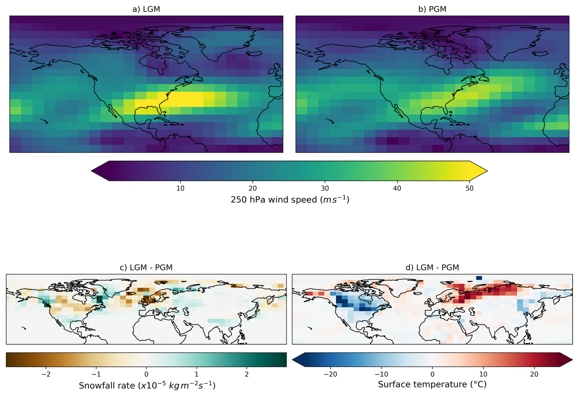
Figure 15 250 hPa DJF wind speed averaged over the last 10 years of NROYa for (a) LGM and (b) PGM. Difference between LGM and PGM (c) DJF snowfall rate and (d) JJA surface air temperature averaged over the last 10 years of NROYa.

Indeed, the simulated climates in this study do show evidence that some of these feedbacks are at play. During winter, the jet stream in the NROYa LGM simulation is stronger and more zonal than in the equivalent PGM simulation, which diplays a weaker and more tilted jet structure over North America and the North Atlantic (Fig. 15a and b). This coincides with increased winter snowfall over the North Atlantic and Northwestern Europe at the PGM compared to the LGM which has a shift in precipitation towards southern Europe (Fig. 5c). These patterns largely agree with previous studies on the impact of Laurentide ice sheet geometry on precipitation patterns (Löfverström and Lora, 2017; Liakka et al., 2016). The summer surface temperature response to the atmospheric circulation changes is less clear since the patterns largely reflect the ice sheet footprints due to the ice-albedo and temperature-elevation feedbacks. However, some additional patterns emerge such as warmer temperatures over Alaska but cooler temperature over Siberia the LGM (Fig. 15d), the latter of which is the opposite of what these previous studies have shown. This highlights that the low resolution of FAMOUS makes it unsuitable for studying the effects of ice sheets on atmospheric circulation in detail (see further discussion in the following section) and any interpretation of these results should be made with this fact in mind.

4.4 Limitations and recommendations for future work

Due to computational constraints, we use a coarse resolution atmospheric model in this study to enable to execution of large ensembles and integration over tens of thousands of years. However, the compromise is that some of the smaller scale atmospheric circulation effects that influence precipitation, temperature and surface mass balance, are not accurately captured. This leads to biases in the modelled climate that contribute to some of the discrepancies between the modelled ice sheets and reconstructions. For example, it has been shown that Atmosphere GCM (AGCM) simulations using horizontal resolutions close to that of FAMOUS (∼ 5.6°), produce lower and smoother topographies, larger southern ablation zones, increased cloudiness and a poor representation of planetary stationary wave effects, compared to resolutions of ∼ 3.8° or higher (Dong and Valdes, 2000; Löfverström et al., 2016; Lofverstrom and Liakka, 2018). These factors can result in substantially warmer summer temperatures over all NH ice sheets, and reduced precipitation over the southwestern parts of the ice sheets. Since the Eurasian ice sheet is particularly sensitive to temperature changes (Abe-Ouchi et al., 2013), this climatology results in the ice sheet model being unable to reproduce the reconstructed western extent of the LGM EIS (Lofverstrom and Liakka, 2018). Therefore, the large negative SMB over Eurasia seen in the simulations presented in this paper, contributing to the unrealistic loss of ice over the British-Irish ice sheet and Scandinavia, may partly be a result of the horizontal resolution used. Similarly, the position of the southern margin of the ice sheets and magnitude of the warm temperature anomaly over northwestern North America has been shown to be dependent on feedbacks between ice sheets and temperatures induced by changes in stationary waves (Liakka et al., 2012; Löfverström et al., 2014; Roe and Lindzen, 2001). Thus, the insufficient southern and eastern margins of the Laurentide ice sheet and the excessive ice growth over Alaska, seen in our simulations, is also partly a consequence of the limited atmospheric resolution. Ziemen et al. (2014) also note that increasing the resolution of their AGCM from 3.75 to 1.9° reduces the cold bias over Alaska, and van Kampenhout et al. (2019) show that refining the grid over the Greenland ice sheet results in improvements to precipitation patterns and the distribution of accumulation. Therefore, the use of a higher resolution atmospheric model would likely result in a closer match to reconstructions. In addition, developing the precipitation downscaling may also help to improve SMB patterns, since currently precipitation is distributed over broad areas of the ice sheet, rather than more realistically concentrated on ice sheet slopes and margins (Smith et al., 2021). A higher resolution atmosphere model and/or the addition of precipitation downscaling would very likely affect the optimal values for the albedo parameters because of the strong influence of snowfall events and frequency on snow albedo.

This study was also limited by the use of prescribed surface ocean conditions and pre-industrial vegetation, and the absence of dust, all of which have been shown to initiate important feedbacks for ice sheet evolution and may improve the configuration of the modelled ice sheets (Ganopolski et al., 2010; Obase et al., 2021; Willeit et al., 2024). For example, the lack of a coupled ocean component means that critical feedbacks involving meltwater forcing and changes in ocean circulation were not explicitly modelled (Obase et al., 2021; Romé et al., 2022). Running fully coupled climate-ice sheet model simulations with a dynamical ocean, vegetation and dust could provide useful information on the role of these other feedbacks on the evolution of ice sheets over glacial-interglacial timescales. However, increasing model complexity can introduce more uncertainty and stronger biases because positive feedbacks can tip the earth system into an unrealistic state. In addition, high resolution is needed to adequately represent some of the interactions not featured here, such as ice-ocean interactions. Indeed, adequately simulating melt in cavities under ice shelves is a challenge even for present-day high-resolution model studies (e.g. Patmore et al., 2023; Berends et al., 2023; Favier et al., 2019). Simulating the effect of ice sheet melt on ocean circulation on millennial timescales is also complicated by internal ocean oscillation mechanisms (e.g. Romé et al., 2025) influenced by Earth's orbit and greenhouse gases (Snoll et al., 2025). Thus, fully coupled atmosphere-ocean-ice sheet model simulations of glacial-interglacial cycles are challenging to set up meaningfully. Prescribing some components of the Earth System, as we have done in this manuscript, presents an opportunity not only to minimise model biases but also to control certain aspects of the state of the Earth System to isolate feedbacks and mechanisms.

5 Conclusions

We ran ensembles of simulations using a coupled atmosphere–ice sheet model under LGM and PGM boundary conditions, varying uncertain climate and ice sheet model parameters. The model simulated plausible Northern Hemisphere ice sheets compared to empirical reconstructions and previous modelling studies, capturing the different configurations between the LGM and PGM. Through Gaussian Process emulation and a Sobol sensitivity analysis, we confirmed that the volume and extent of both the simulated Northern Hemisphere ice sheets are mostly sensitive to the parameters that control their albedo. However, the North American ice sheet and the Eurasian ice sheet, and the 2 glacial maxima, displayed different sensitivities to other parameters. The size of the Eurasian ice sheet is more sensitive to parameters controlling basal sliding and clouds/precipitation than for the North American ice sheet. We also find that the sensitivity to parameters controlling sliding and surface mass balance can depend on the size of the ice sheet at each glacial maxima.

We described 2 sets of Not Ruled Out Yet (NROY) parameter values compatible with reconstructed extent and volumes for both periods and both ice sheets, and we highlight 2 additional simulations that we deem NROY depending on the criteria used. Improvements in our model setup produce a good match to empirical reconstructions of LGM ice streams, especially in simulations with lower values of till water drainage rate (drain).

The 4 NROY simulations produced in this study provide a means for other studies to evaluate the effect of ice sheet uncertainty on climate and sea levels. They also provide new and improved initial conditions that can be used for simulating and comparing the Last and the Penultimate deglaciations, which will be the focus of future work. However, since it has been shown in the past that models can be overtuned to certain climate conditions, it is not guaranteed that these parameter values will be conducive to the deglaciation of the ice sheets in line with empirical reconstructions and work will need to be done to test this and calibrate the model for both past and present conditions which will likely involve the use of emulators. In addition, there are some factors that were not considered or simplified in this work that may become more important for the deglaciation. These include: the ice shelf melt parameterisation (Berends et al., 2023), the resolution at the grounding line (Gandy et al., 2019) and the representation of proglacial lakes (Sutherland et al., 2020).

By performing a systematic calibration of our coupled climate-ice sheet model to reconstructed LGM ice extent and volume and simultaneously applying it to the PGM, we produced new reconstructions of the North American and Eurasian ice sheets at the Penultimate Glacial Maximum, greatly improved compared to previous work and informed by climate and ice sheet physics and geological data. Our PGM reconstructions can be used to model or study the climate, ice sheet dynamics, the solid earth and sea levels.

Appendix A: Implementation of the elevcon parameter

elevcon affects the surface temperature and SMB during the height adjustment to ice sheet tiles in the following manner;

• The effective elevation of each tile is multiplied by the value of elevcon. A value of 1.10 (10 %) means that the elevation of an 1800 m tile has been increased to 1980 m.

• Surface air temperatures and longwave radiation are downscaled to each increased elevation tile.

• Surface fluxes and SMB are calculated based on the downscaled variables and other variables from the original FAMOUS grid.

• The SMB and fluxes are then passed to the ice sheet and atmospheric models, but taken to represent the original tile elevation, not the increased elevation to which the surface temperature was actually downscaled. For example, the surface air temperature and SMB could be calculated on a 1980 m elevation tile, but they will be passed to the ice sheet and atmospheric models as outputs from an 1800 m elevation tile.

Therefore, the increase in the tile elevation is only accounted for during the downscaling of surface temperature but is not reflected when passing it to the ice sheet model or elsewhere in FAMOUS. In this way, additional cooling is applied over the ice sheet interior by elevcon, which can be regarded as elevation-dependent height adjustment over ice sheets. This crudely mimics the effect of the stable boundary layer in maintaining the cold surface condition in that area.

Two types of sensitivity experiments are performed with FAMOUS-BISICLES to validate the effect of elevcon on the modern and LGM ice sheets and climates. The first sensitivity experiment is conducted under modern climate and the Greenland ice sheet based on a control simulation performed by Lang et al. (in prep) and focuses on the effect of elevcon on the SMB. As shown in (Smith et al., 2021), the model simulates a mean ELA of approximately 1.8 km over the Greenland ice sheet, whereas high resolution regional atmospheric models (e.g. MAR; Fettweis et al., 2013) suggest 1.2 km, meaning that the model overestimates the ELA by 50 % (Fig. A1). Here, we applied an elevcon value of 50 % and rerun the simulation. The inclusion of the elevcon adjustment strongly suppresses the negative SMB seen around the elevation of 1 to 2 km, and the ELA drops from 1.8 km to approximately 900 m height (Fig. A1). Given that the ELA is now underestimated compared with the high resolution models, the value of 50 % appears to be too large and can be regarded as the upper limit. However, this sensitivity experiment clarifies the substantial effect of elevcon on the SMB at the interior of the ice sheet. It further shows that elevcon can be used to explore the effect of uncertainties in the SMB at the interior of the ice sheet arising from underestimating the role of the stable boundary layer.

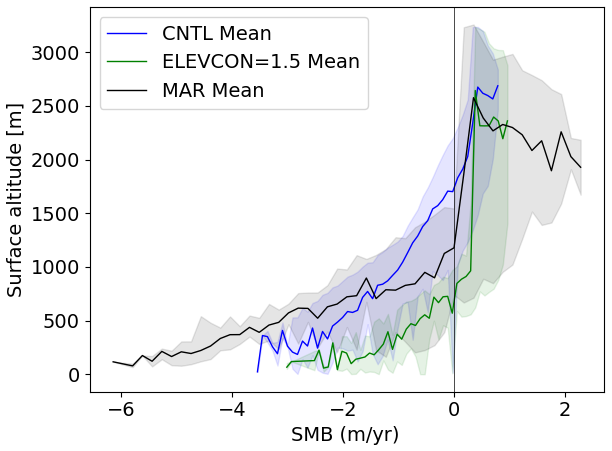
Figure A1 Relation of SMB and surface altitude over the Greenland ice sheet in the modern climate simulations with FAMOUS-BISICLES. The blue line (shading) shows the mean result (range) from the control experiments, and the green shows those from the sensitivity experiments that include elevcon with a value of 1.5 (50 %). Also shown in black are the results from simulations using the MAR regional climate model (Fettweis et al., 2013).

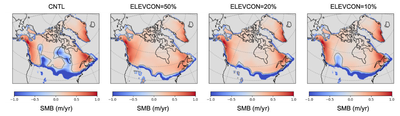
Figure A2 Effects of different magnitudes of elevcon on the spatial pattern of SMB over the North American ice sheet at the LGM. CNTL corresponds to 1 of the ensemble members (xppma) in Sherriff-Tadano et al. (2024).

The second type of sensitivity experiments are performed under the LGM climate for the North American ice sheet. Here, values of 10 %, 20 % and 50 % are tested with 1 of the ensemble members from Sherriff-Tadano et al. (2024) that exhibits a strong local melting of the ice sheet from parts of the interior. Results are shown in Fig. A2. The strong local melting observed around the Hudson Bay region in the control simulation is removed in all the sensitivity experiments. Also, depending on the magnitude of the value of elevcon, the negative SMB seen at the eastern part of the Rocky Mountains is reduced and pushes the ELA southwards.

Appendix B: BISICLES spin-up

The internal temperature of ice sheets is an important factor in controlling the deformation, rheology and velocity of the ice due to the temperature dependence of the sliding law and enthalpy scheme (Blatter et al., 2010). The ice sheets start with a uniform internal temperature of 268 K and it can take tens of thousands of years for the process of cold ice advection from the interior and heat conduction from the bed to occur and reach an equilibrium, which is important for the formation of ice streams (Fyke et al., 2014; Heine and Mctigue, 1996). Thus, we perform ice sheet model only spin-ups for the LGM and the PGM to allow the ice sheet internal temperatures to reach close to equilibrium. This temperature profile is then used as the internal ice sheet temperature in the initial condition for the sensitivity tests (Appendix C) and coupled simulations.

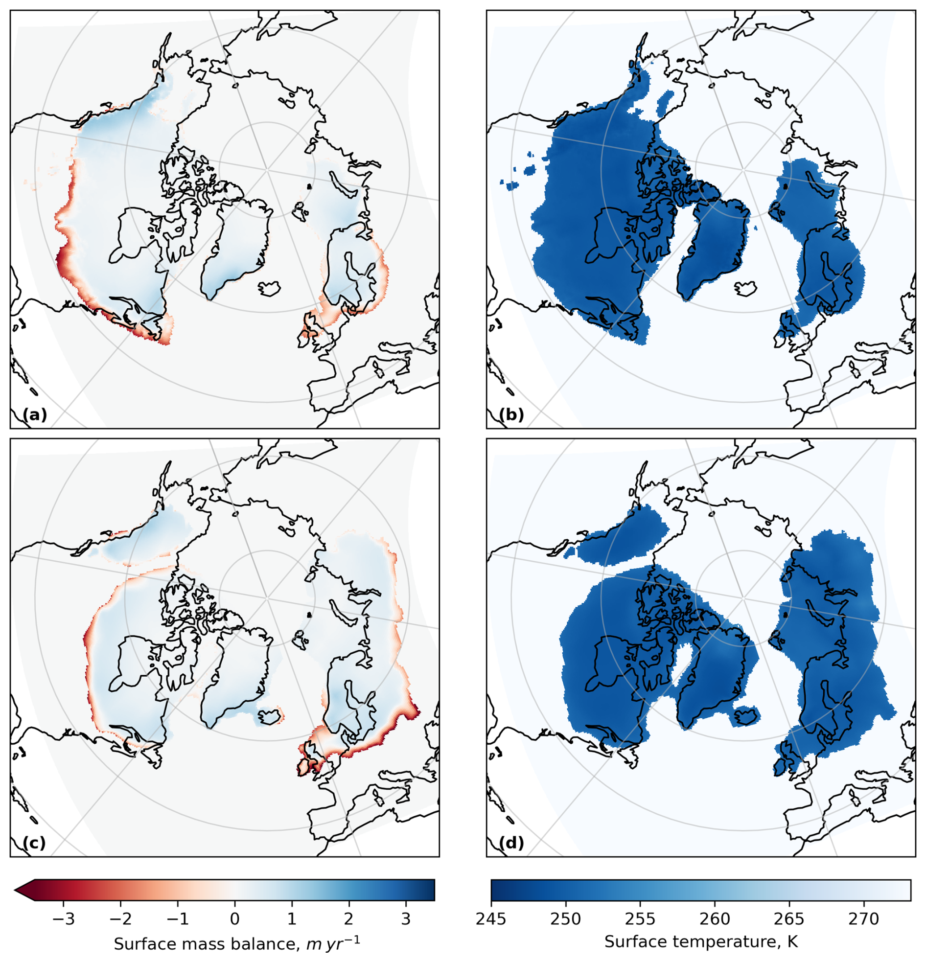
Figure B1 Surface mass balance and ice surface temperature fields used in the (a), (b) LGM and (c), (d) PGM spin ups.

The spin ups were run at 32 km resolution for 20 000 years using single surface mass balance and surface temperature fields taken from a FAMOUS-BISICLES equilibrium simulation that used climate model parameters identified to be NROY in simulations of the NAIS by Patterson et al. (2024), default ice sheet model parameters and an elevcon value of 1.2 (Fig. B1). The initial ice sheet configurations were the same as used in the coupled simulations (described in Sect. 2.3.1; Fig. 1). The sliding law was set to a temperature dependent Weertman sliding without till water dependent Coulomb sliding enabled since the bulk of the temperature field is not affected much by Coulomb sliding near the coast. The resulting temperature profiles are shown in Figs. B2 and B3.

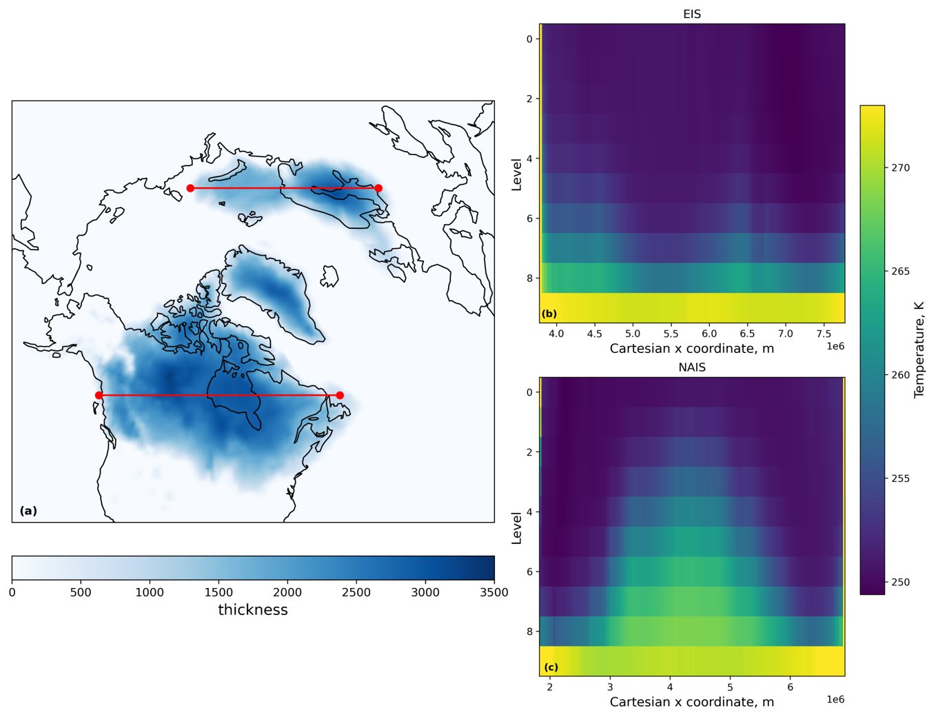
Figure B2 Cross section of LGM ice temperature at the end of the 20 000 year spin-up for the transects indicated by the red lines in (a), for the Eurasian ice sheet (b) and the North American ice sheet (c).

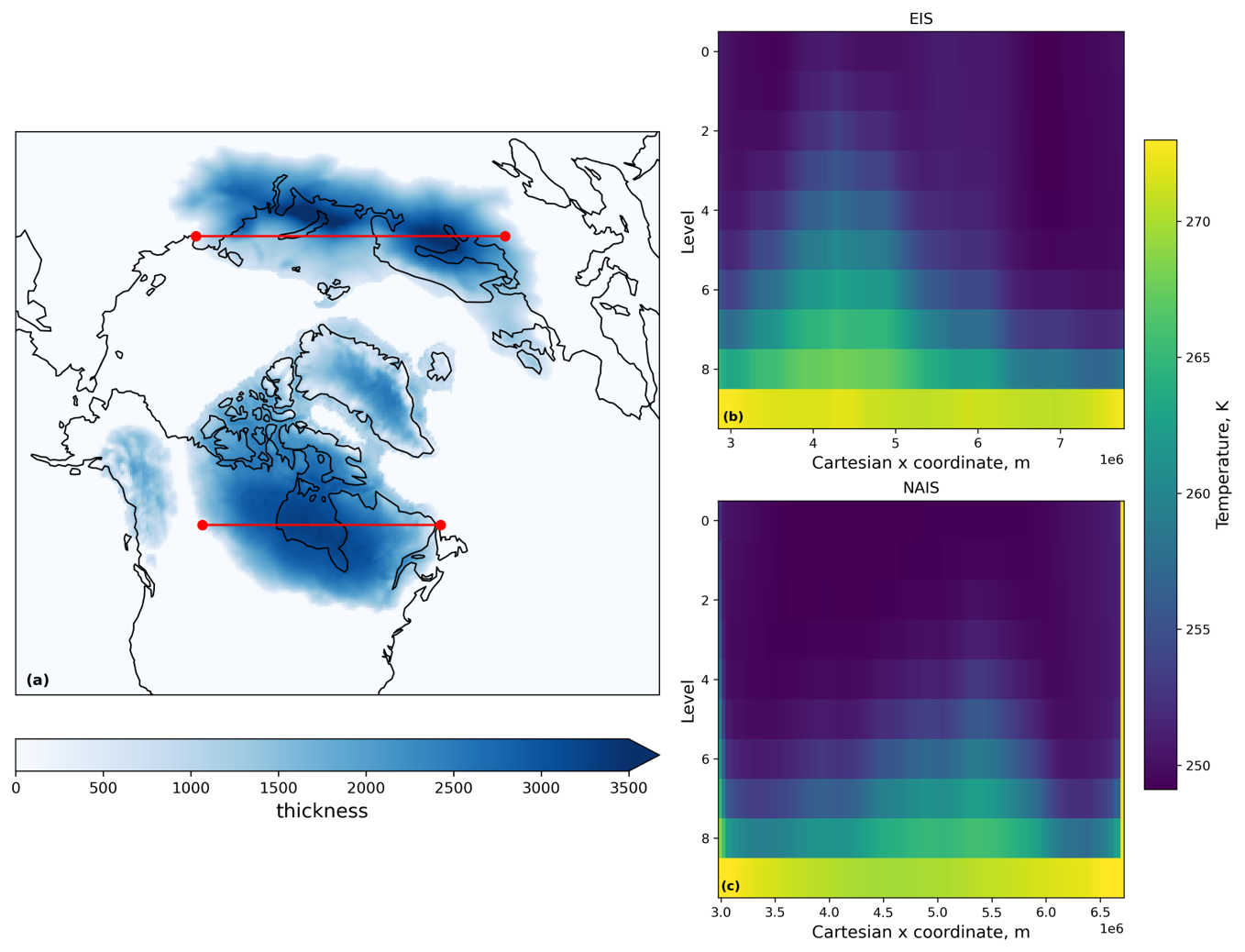
Figure B3 Cross section of PGM ice temperature at the end of the 20 000 year spin up for the transects indicated by the red lines in (a), for the Eurasian ice sheet (b) and the North American ice sheet (c).

Appendix C: Sensitivity tests

In their study, Sherriff-Tadano et al. (2024) used much higher values of drain (0.2–0.6 m yr⁻¹) than has typically been used in previous studies (0.001–0.005 m yr⁻¹; Gandy et al., 2019; Kazmierczak et al., 2022; Moreno-Parada et al., 2023). This was to prevent large till water depths leading to too large velocities across the entire ice sheet and long simulation times, as high velocities require more iterations and smaller timesteps to solve. This resulted in the till water drainage outpacing the supply and thus very small till water depths, leading to mostly Weertman sliding across the whole ice sheet.

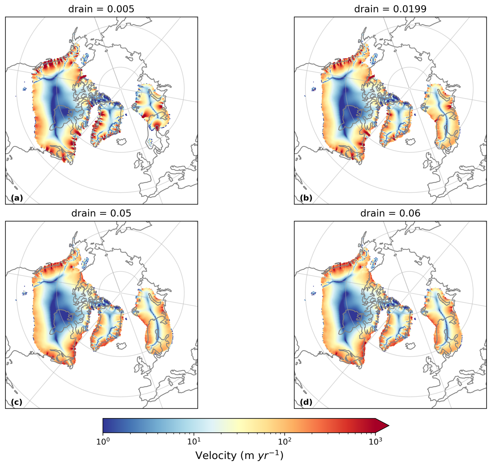
Figure C1 Ice velocity after 5000 ice sheet years in simulations using till water drainage rates of (a) 0.005 m yr⁻¹, (b) 0.0199 m yr⁻¹, (c) 0.05 m yr⁻¹ and (d) 0.06 m yr⁻¹. All other parameters and initial conditions were kept the same.

Slow till drainage (low values of drain) can lead to isolated regions of fast flow, > 50 km yr⁻¹, which have a disproportionate effect on simulation time. To prevent this we introduce an artificial drag term rising with the fourth power of ice speed and calibrated to be negligible for ice speeds below 1 km yr⁻¹. This drag factor is also used in the coupled simulations throughout the rest of this study. We then perform sensitivity tests with different values of drain spanning the range 0.001–0.06 m yr⁻¹ but all other factors kept constant. The results of some of these tests are shown in Fig. C1. Values of drain above 0.05 prevent much of the coulomb sliding at the coasts and the representation of some of the major ice streams, particularly the Hudson Strait Ice Stream, is poor. Low values usually used in ice sheet models (0.001–0.005) cause too large velocities and ice streams that remove much of the ice sheet, especially in Eurasia. Therefore, in this study, we implement a range of 0.01–0.05 to cover values just below the default till water supply rate of 0.02, to where no coulomb sliding occurs. For studies that seek to examine ice streaming of the glacial maximum ice sheets, we would recommend performing additional sensitivity tests that vary ice shelf basal melt parameterisation and geothermal heat flux, but this is beyond the scope of the present study.

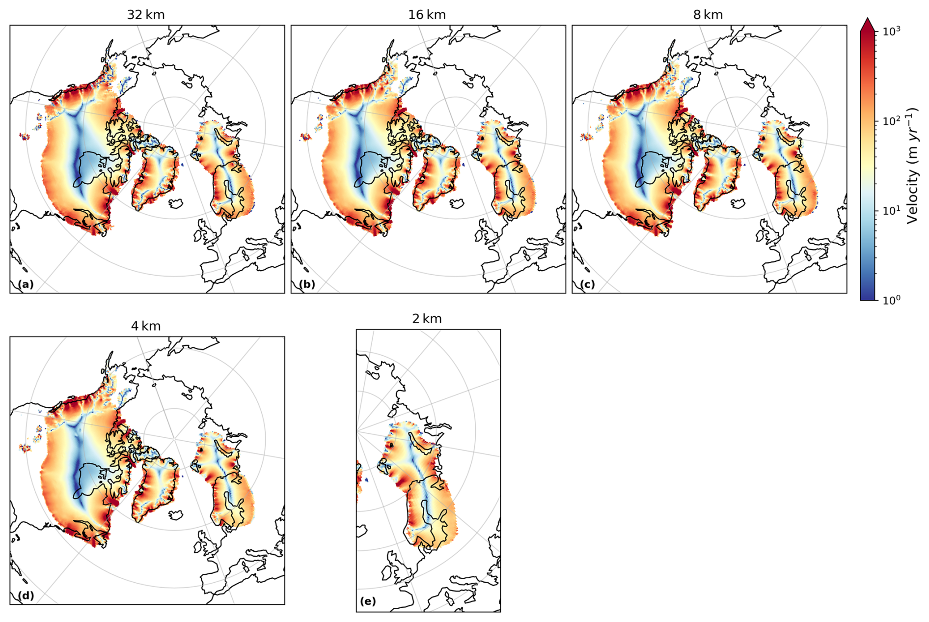
Figure C2 Ice velocity averaged over the 5000 year simulations using different levels of ice stream refinement. All areas covered by ice were refined to 16 km in panel (b); the ice sheet remains at 16 km and only areas of ice streaming are refined to the finer resolutions indicated in panels (c)-(e). Only the ice streaming across the marine section (BKIS) was refined on panel (e).

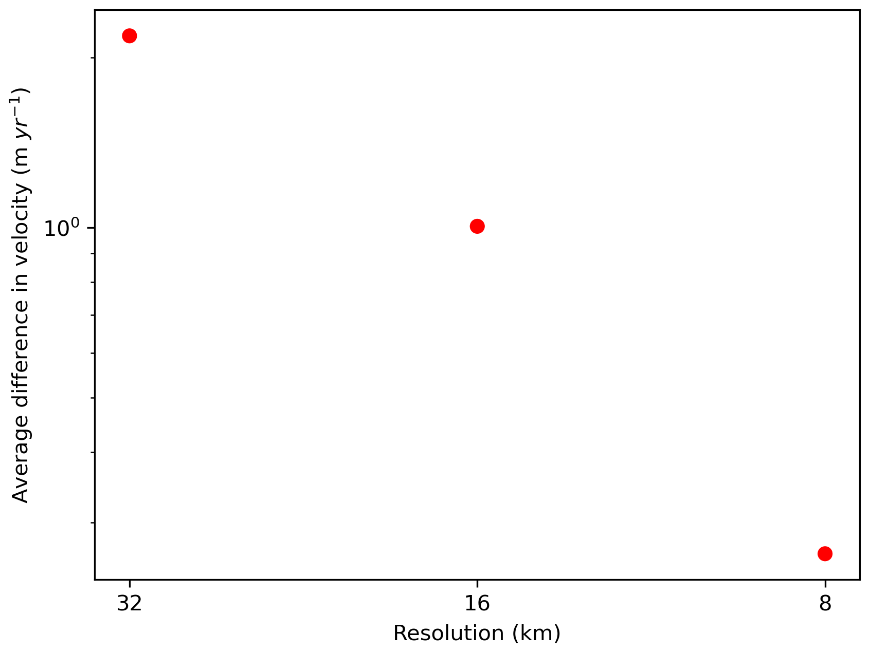
Figure C3 Difference in ice velocity averaged over the whole ice sheet and 5000 year simulations between the 4 km resolution simulation and higher resolutions (8, 16 and 32 km).

The base resolution of the ice sheet model is 32 km. The AMR allows the areas covered by ice to be refined once to 16 km, which shows some improvement to the simulated ice streams, although the difference is only about 1.2 m yr⁻¹ on average over the whole ice sheet (Fig. C2a and b). Additional sensitivity simulations were performed refining only the areas of ice streaming up to 8 km and up to 4 km (Fig. C2c and d). These tests showed that after refining the entire ice sheet to 16 km, the difference in average ice velocity for any further refinement of the ice streams converges to zero (Fig. C3) and the pattern of major ice stream features (Fig. 2), the position of the marine margins and the ice volume across the NH ice sheets is not significantly changed, except across the southern area of the Eurasian ice sheet (Fig. C4). However, computational costs are quadrupled with each level of refinement. Thus, we determine one level of refinement (16 km) to be sufficient for this study in which we are focussing more on the large-scale geometry of the ice sheet rather than the finer details of the ice streams. This is a similar conclusion to that drawn from the simulations presented by Albrecht et al. (2020) and Gandy et al. (2019), the latter further showing anything finer than 4 km does not improve the match of simulated ice streams to empirical data over the British Isles.

There is an increase in the velocity of up to around 3000 m yr⁻¹ at the centre of some of the ice streams at the higher resolutions, which could be important during simulations of the deglaciation (Robel and Tziperman, 2016). We performed an additional simulation refining the ice streams across the marine section of the Eurasian ice sheet to 2 km to see if any marine processes would be captured that could not have been resolved at lower resolutions. This did not lead to any significant difference in the ice velocity in this region compared to the 4 km simulation (Fig. C2e), but again could be important in deglaciation simulations when MISI could be triggered (Gandy et al., 2021; Patton et al., 2015; Petrini et al., 2020; van Aalderen et al., 2024).

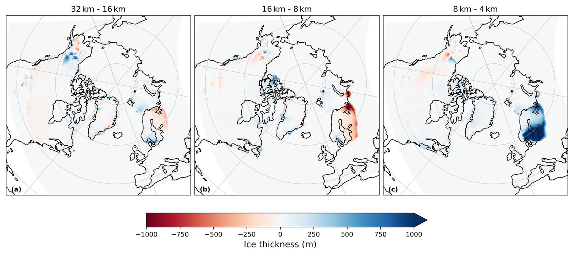
Figure C4 Difference in final ice sheet thickness between simulations with different levels of refinement

Appendix D: Leave-one-out-cross-validation (LOOCV)

Whilst a large proportion of the predicted diagnostics matched the modelled values within the 95 % credible interval, the LOOCV reveals that the Gaussian Process emulator struggled the most with predicting smaller ice sheet volumes and areas. This was especially the case for the PGM Eurasian ice sheet where many of the simulations collapsed due to GIA feedbacks and non-linearities in ice sheet-climate interactions. There is also one obvious outlier in all 8 of the diagnostics where the emulator predicted a much higher value than what was actually modelled. This is the same parameter set (xprrk/xpruk) for each.

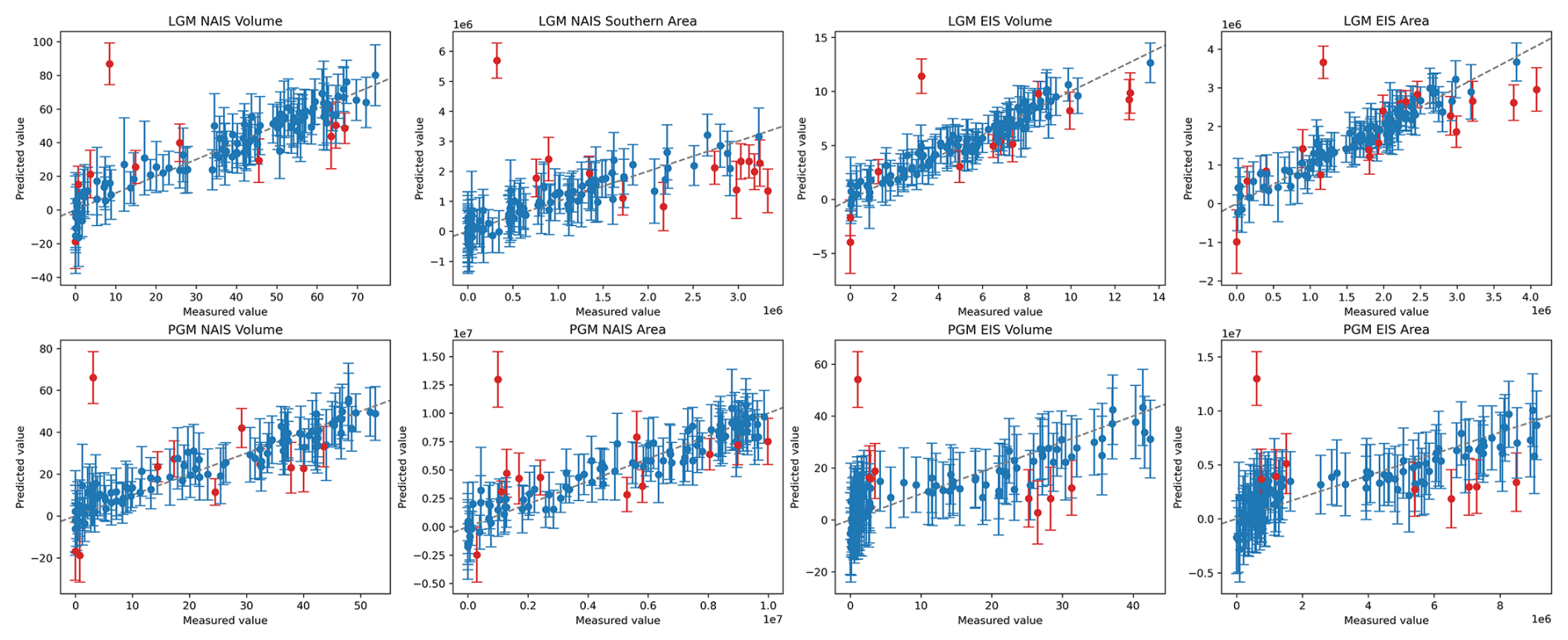
Figure D1 The results of the Leave-One-Out Cross Validation performed on emulators for the 8 diagnostics. The points show the value produced by the numerical model against the value predicted by the emulator for the same sets of input parameters. The line through the centre is the 1:1 line and the error bars show the 95 % credible interval for each point. The points for which the measured value does not fall within the error bars are highlighted in red.

Appendix E: Time series of diagnostic variables for NROY simulations

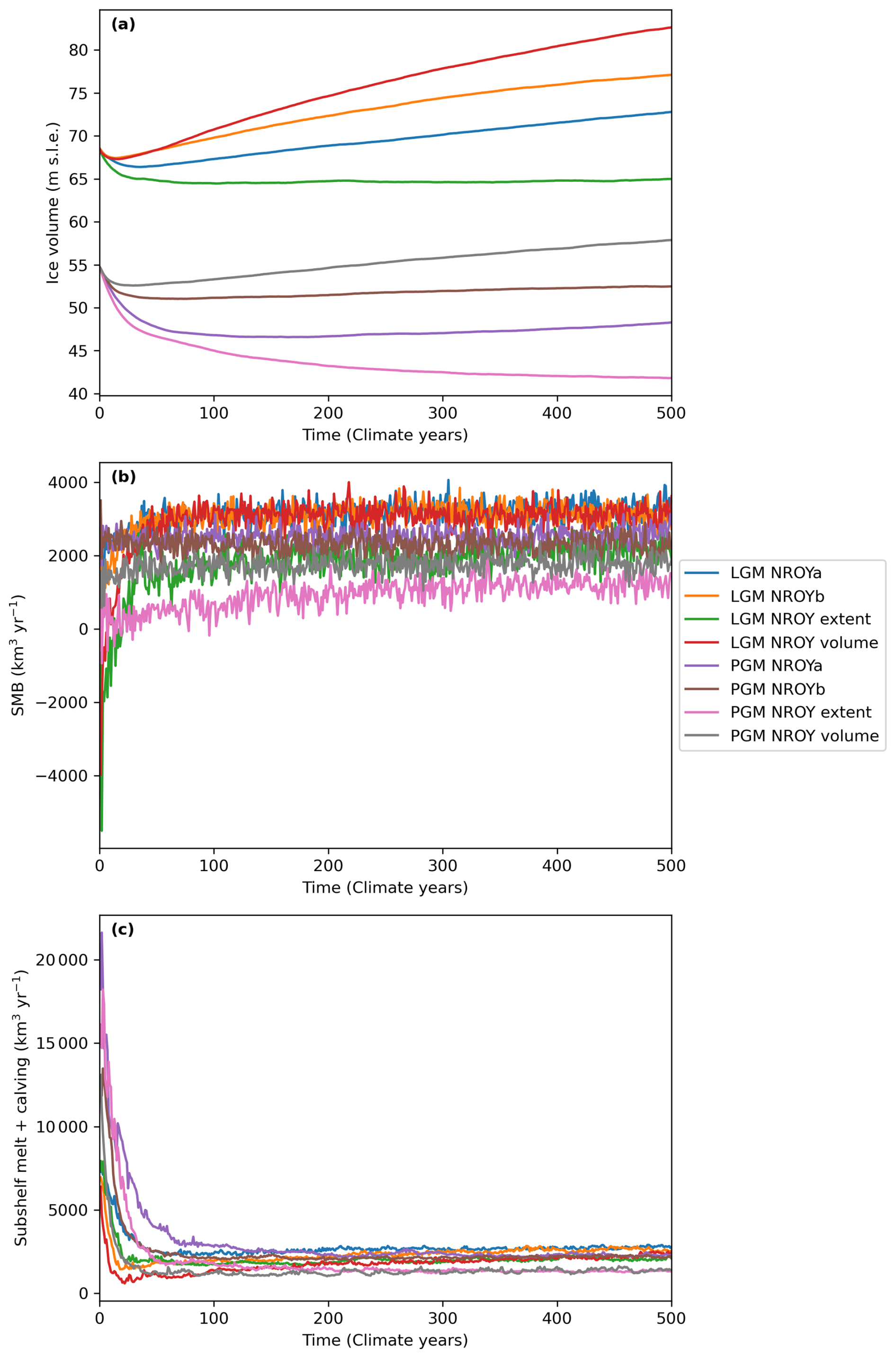
Figure E1 Time series of variables averaged over North America for the NROY simulations; (a) ice volume; (b) surface mass balance; (c) total sub-shelf melt plus calving mass loss; and (d) surface air temperature.

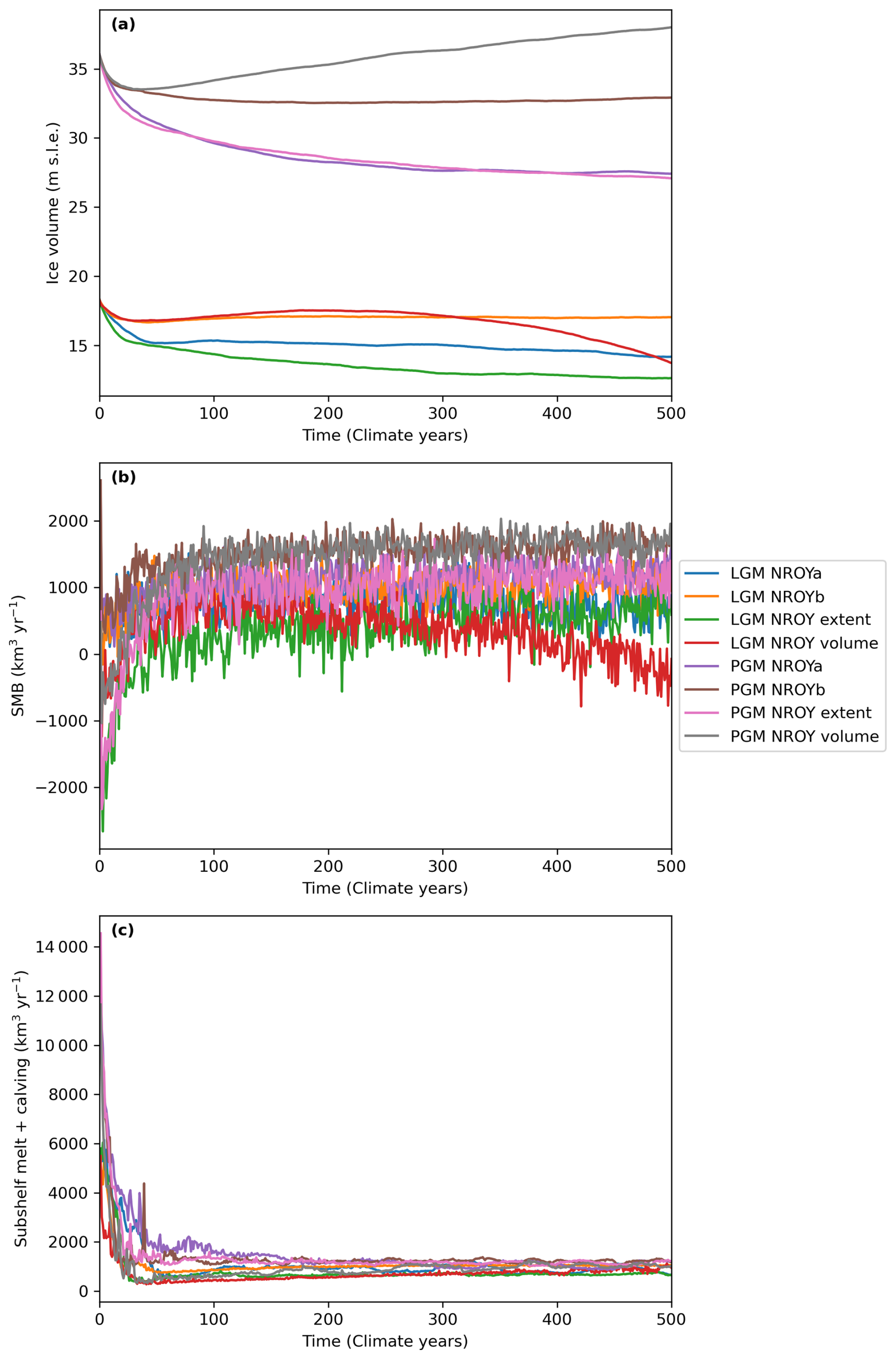
Figure E2 Time series of variables averaged over Eurasia for the NROY simulations; (a) ice volume; (b) surface mass balance; (c) total sub-shelf melt plus calving mass loss; and (d) surface air temperature.

Appendix F: Parameter pair plots

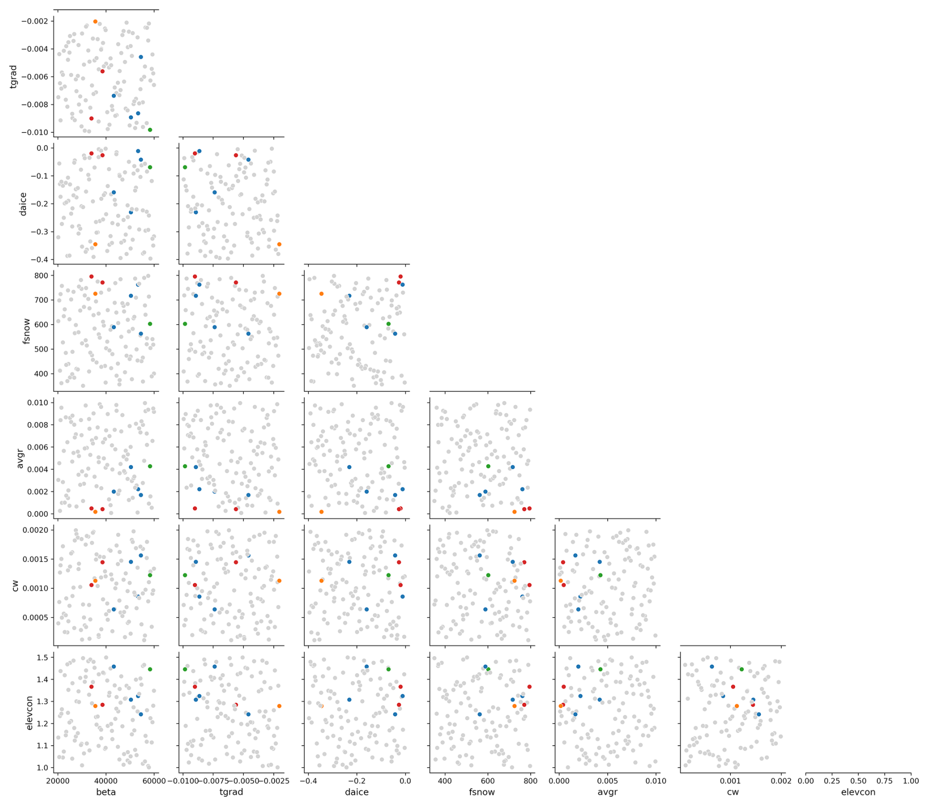
Figure F1 Parameter pair plot of the most influential parameters with the NROYa and NROYb simulations in red, NROY extent simulation in orange, NROY volume simulation in green and the 4 other simulations that meet the North American ice sheet constraints but not the Eurasian in blue.

Appendix G: PGM ice streams

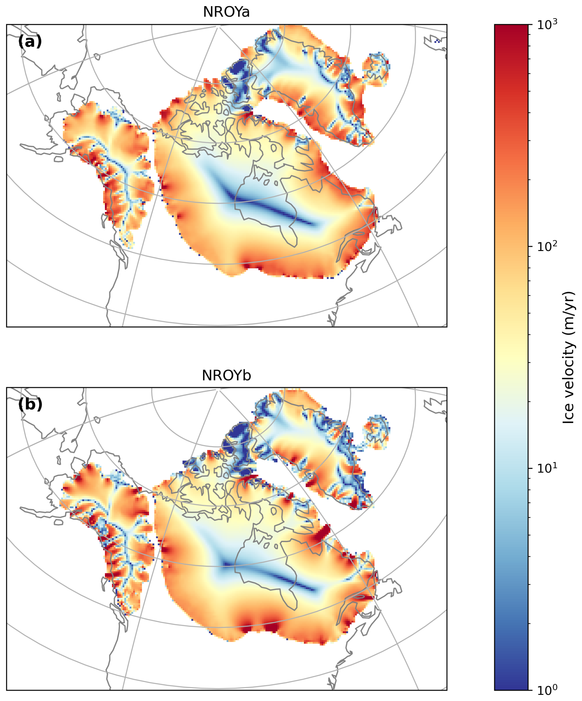
Figure G1 North American ice sheet ice velocity at the end of the 5000 ice sheet years for the 2 equivalent PGM NROY simulations

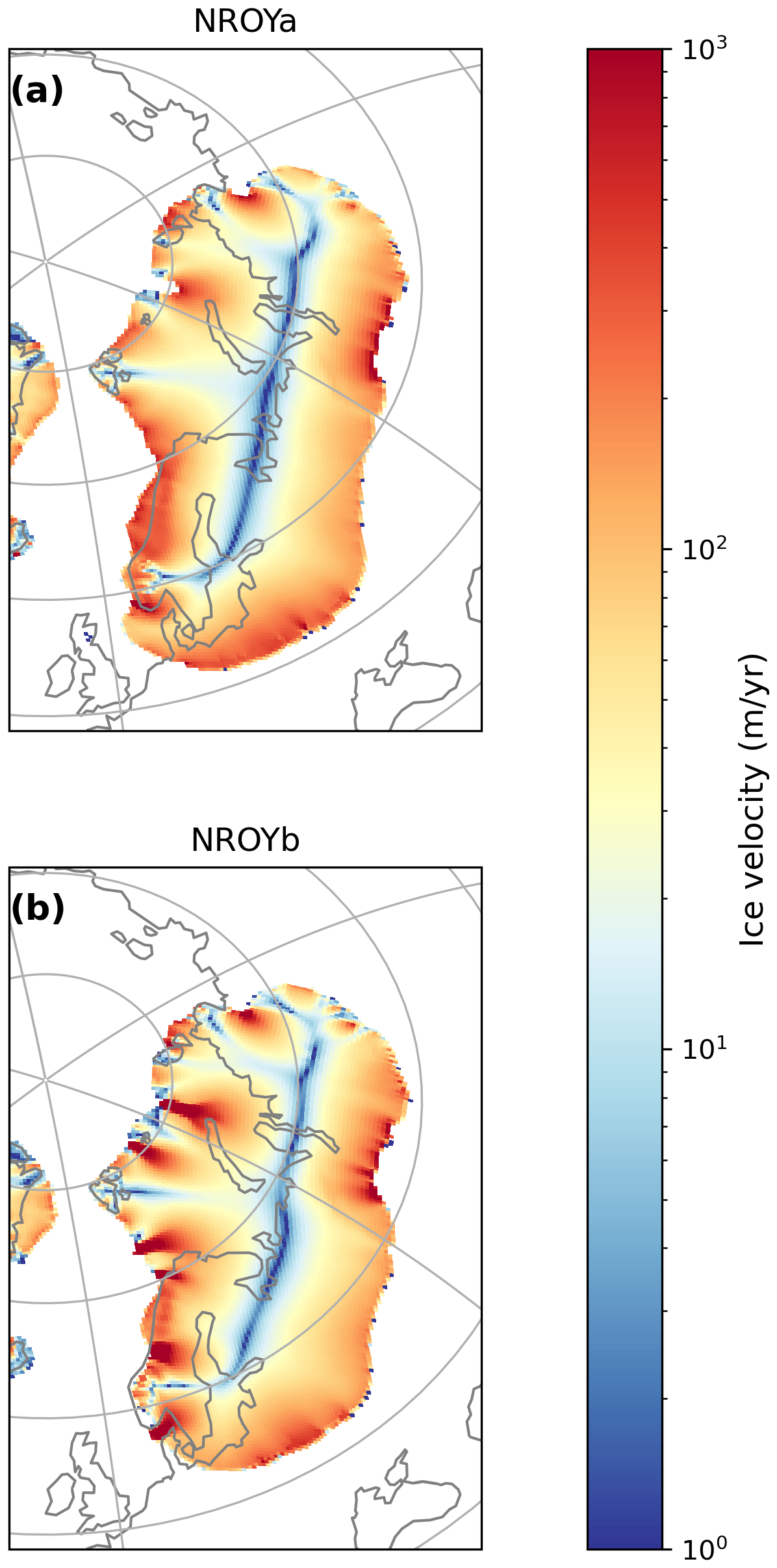
Figure G2 Eurasian ice sheet ice velocities at the end of the 5000 ice sheet years for the 2 equivalent PGM NROY simulations