Understanding slow glacier flow under climate change: A case study on Vernagtferner, Austria

Long-term surface velocity observations of glaciers reflect the dynamics of glacier ice and its interaction with the mass balance, including variations due to climate change. In this study, we investigate the surface velocities of a slow-flowing glacier which is influenced by strong surface melt and negative mass balance during the last decades. The annual stake measurements date back to 1966 and allow the study of ice dynamics for more than five decades. We observed a strong relationship between the surface velocity and ice thickness, especially in the case of the glacier^′s response to thinning. A series of slightly positive mass balances led to a minor glacier advance around 1980, associated with a considerable speed-up of the glacier. With the onset of the negative mass balances, the velocity has decreased steadily until today. Our results suggest that the displacement of ablation stakes response relatively direct to changes in surface mass balance. The surface mass balance is currently the dominant control for geometry change, while local dynamic contributions to elevation change remain secondary. Based on recent in situ measurements, a seasonal variation of surface velocities can be identified, with around 30 % higher summer velocities in relation to the annual average. In order to investigate the current ice surface flow, we aimed to derive a spatially distributed velocity map. The combination of low ice flow and high ablation challenges the use of standard remote sensing techniques, as ablation induced changes overlay the displacement of surface features. We therefore relied on manual feature tracking based on unpiloted aerial vehicle (UAV) surveys, and airborne imagery, and combined the results with stake measurements to generate a dataset for the period 2018–2023. With an average velocity of 1 m yr⁻¹ and a maximum displacement rate of 4 m yr⁻¹ in the central part of the glacier, it gives a clear picture of the low present-day glacier flow.

1 Introduction

Mountain glaciers move downwards due to internal deformation and, in most cases, basal sliding, induced by the surface slope and gravitational forces. They act as a delayed response to climate change by translating changes in the mass balance into area changes modulated by the ice flow (Heid and Kääb, 2012; Mayer et al., 2013b). The glacier surface velocity, which can be measured using field or remote sensing techniques, is based on two components: internal deformation of the ice, predominantly due to shear stress and basal sliding at the glacier bed. The glacier surface velocity and its impact on glacier dynamics have been investigated in several studies. For instance, surface velocity changes may provide valuable information on hydrological conditions, including subglacial water pressure and drainage system evolution (Iken, 1981; Mair et al., 2002), on variations in meltwater production (van de Wal et al., 2008) and on changes in glacier geometry and topographic conditions (Heid and Kääb, 2012; Thomson and Copland, 2017). Thus, glacier velocity serves as a key indicator of multiple processes within the glacier system. Understanding these velocity pattern and their temporal changes on a resolution considerably higher than the spatial variability is increasingly important, particularly for capturing variations in glacier processes. Therefore, long-term measurements of the ice velocity are essential for detailed analyzes. A long time series of measurements makes it possible to investigate the flow processes of a glacier and their response to climate change. For example, Vincent and Moreau (2016) found no correlation between changes in surface velocity and subglacial water runoff for the Argentière glacier in the Mont Blanc area. On the other hand, mass balance influences the flow behavior, where Vincent et al. (2009) found a reaction of glacier velocities within a maximum time span of three years. However, ice geometry variations and surface velocity evolution are not always directly correlated. For example at glacier de Saint Sorlin, Grandes Rousses area, velocities around the year 2000 are still larger than in 1960, despite a negative cumulative net mass balance since 1957 (Vincent et al., 2000). This shows the complexity of the processes involved. Spatial high-resolution velocity information as well as long-term monitoring allow a reliable analysis of glacier behavior.

There are several methods to measure glacier surface velocities. A method established by Nye (1959) measures the displacement of stakes installed at the surface over a period of time to determine the strain rate. This is a very labour-intensive in situ method, where stakes are placed in boreholes in order to track the movement of the glacier surface. The advantage of this traditional in situ method is the accuracy of displacement measurements over months and years, providing seasonal or annual ground-truth measurements of surface displacement. The disadvantage is the limited spatial coverage due to the point measurement approach, which is further restricted to accessible glacier sections. In addition to traditional methods, modern remote technologies offer ways to estimate glacier velocities efficiently with large spatial coverage. For instance, data acquired by air- or space-borne sensors and UAVs (unpiloted aerial vehicles) can be used to derive glacier surface velocities by using different tracking approaches.

The further development of UAVs offers an economical and simple method to obtain data from a specific area in the desired temporal and spatial resolution. Previous applications are described in detail in Gaffey and Bhardwaj (2020). Despite their great potential, UAV-based methods also have certain limitations, such as flight time and distance or dependence on weather conditions, especially in the low-cost and open-source software sector, as demonstrated by Groos et al. (2019). Such as UAV measurements, airborne data makes it possible to estimate ice surface velocities over a large spatial area. A variety of sensors, including aerial imagery (Leprince et al., 2008), SAR (synthetic aperture radar) interferometric (Prats et al., 2009) and LiDAR (light detection and ranging) (Arnold et al., 2006) can be applied.

Space-borne remote sensing data can be utilized to estimate ice velocity of mountain glaciers and in particular of polar ice sheets (Dirscherl et al., 2020). However, these methods have certain limitations, such as temporal and spatial resolution, the need for recognizable features, or maintained coherence across acquisitions. In their investigation across several regions, Millan et al. (2019) showed that Sentinel-2 data can produce more precise results than Landsat-8. Global datasets, like FAU's glacierportal (Friedl et al., 2021), ITS_LIVE (Gardner et al., 2022) or a dataset published by Millan et al. (2022) offer user-ready velocity products, providing comprehensive coverage and accessibility for glaciers worldwide. For individual glaciers, better results can be achieved with specific optimized data processing than with global data sets (Mattea et al., 2025). Even relatively low ice velocities can be detected, as Gindraux (2019) shows for Griesglacier. However, slow-flowing glaciers need specific temporal baselines between image pairs to capture recognizable flow. This implies a potential loss of coherence, as surface features (e.g. crevasses) can change considerably during this period (van Wyk de Vries and Wickert, 2021).

The aim of our study is to investigate in detail the ice dynamics of the slow-flowing glacier Vernagtferner. Therefore, we use long-term, systematic ice velocity measurement information from 1966 to present for analyzing the ice flow and its variability in relation to the also observed mass balance/ice geometry time series. In addition, we aimed on providing a map representation of current ice flow, in order to demonstrate the low-flow character of the glacier, with its specific variability. We decided to use manual feature tracking, after highlighting the challenges associated with high ablation for retrieving glacier velocities on slow-moving glaciers with remote sensing techniques. The resulting map of current velocities, combined with the long-term ice dynamics information, supports modeling of alpine glaciers and a plausibility assessment of future remote sensing datasets and methods.

2 Study site

The study was carried out on the slow-flowing (Mayer et al., 2013b) alpine glacier Vernagtferner (VF), located in the southern Oetztal Alps, Austria. The glacier covers an area of approximately 6 km² and is still one of the largest glaciers in Austria, with an altitude ranging from around 2900 to about 3500 $\mathrm{m}\mathrm{a}.\mathrm{s}.\mathrm{l}.$. VF was selected based on its extensive data availability, suitable for this study. The data archive of VF covers over 130 years of observations, beginning with the first topographic map of the glacier in 1889 generated by Sebastian Finsterwalder (Finsterwalder, 1897). At VF, continuous monitoring of mass balance and surface velocity started in 1966. Negative mass balance persisted for the last 35 years (WGMS, 2024). The neighboring glaciers Kesselwandferner and Hintereisferner have also been observed in detail, starting in the 1950s. Together, VF, Kesselwandferner, and Hintereisferner forming a well-monitored site of glacier-related variables. A detailed overview of the available data sets and measurements is presented in Strasser et al. (2018). VF can be divided into three areas: the western part, called Schwarzwandzunge, which has to be regarded as an independent part since 2006 as a result of the strong glacial retreat in recent decades, the middle part, known as the Taschach area, and the Brochkogel area in the eastern part (Mayer et al., 2013a). Although Schwarzwandzunge disconnected from the main part, it is still considered as part of VF in order to maintain consistent mass balance measurements of VF over the years. A detailed study (Reinwarth and Escher-Vetter, 1999) of the mass balance of the three areas indicates that the Schwarzwandzunge area behaves fundamentally differently from the rest of VF, presumably due to the different area-elevation distribution. Overall, for the period 2016–2023, the SMB at Brochkogel is approximately 20 % less negative than in the Schwarzwand and Taschach area (BAdW, 2026).

3 Data and methods

3.1 Overview of datasets and general workflow

This study investigates glacier dynamics at VF over more than five decades (1966–2023) and provides additional insights into the spatially distributed velocity field of the recently observed period (2018–2023). Long-term in situ stake measurements provide the basis for observing historical changes in surface velocity, even well before the beginning of observations from satellite data. Furthermore, the surface mass balance (as a single value) is known for the same period of time. DEMs (digital elevation models) are available at different times. An uninterrupted timeline of the geometry can be generated using interpolation. From these DEMs, surface slope and ice thickness (based on the measured topography of 2006) can be derived on an annual basis. The methodological workflow for calculating ice thickness and surface slope is shown in Fig. 2. The current velocity map is generated manually after reviewing existing standard remote sensing products and techniques, which we also describe in this manuscript. A detailed overview of all used datasets (long-term and recent data) can be found in the Supplement.

3.2 Stake measurements as a long-term data source

A network of stake measurements has been established on VF since 1966. The primary objective of these measurements was the observation of surface ablation and thus the stakes are primarily located in the ablation area (Fig. 1). Therefore, the stake positions are in general not completely representative for capturing ice surface velocities across the entire glacier. Note that the stake network was adapted over the years to capture the ablation area which changed over time due to the propagation of ablation to higher elevation in response to global warming. For this reason, the elevation range captured by the stake network varies. The locations of the stakes were measured once a year at the end of the hydrological year (end of September), together with the ablation measurements. This allows the calculation of the annual surface velocity. The measurement series are usually interrupted due to melt out of the stakes. However, the stakes are then re-drilled very close to the melt out location, so that the flow can be monitored.

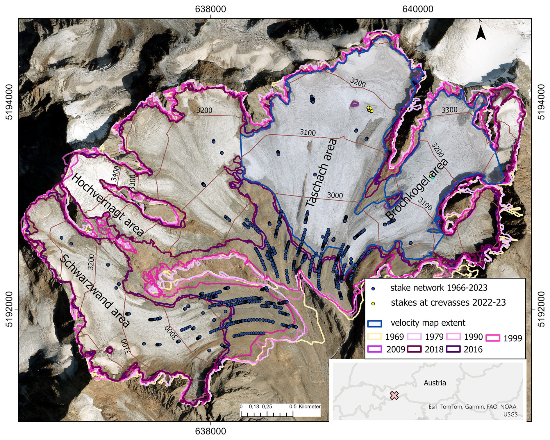
Figure 1 Study area Vernagtferner in the Oetztal Alps with different glacier extents (from 1969–2018) and the velocity map extent as coloured outlines. In addition, stake locations are provided from the long-term observations, as well as from the short-term crevasse observations as dots. Background image: Orthoimage © Land Tirol 2022.

Over time, different coordinate systems were used as a basis for the measurements. Meanwhile, a local system is used, which is closely aligned with the UTM (Universal Transverse Mercator), and all former measurements have been transformed into this system. Additionally, the methods for determining stake positions changed over time, starting with multiple forward intersections, continuing with terrestrial polar coordinate method, and using GNSS (global navigation satellite system) positioning for a certain period (Tremel et al., 1994). The derived velocities have been displayed in previous studies up to the respective point in time (Hirtlreiter G., 1985; Khazaleh, 2002).

In addition to the systematically monitored stake-network, 11 stakes were installed in actively moving sections of the glacier in the Taschach and Brochkogel area during the period 2022–2023. The stake positions were measured several times (4 August 2022, 10 July 2022, 21 September 2022, and 8 August 2023), allowing an analysis of seasonal variations in ice flow. VF is very likely a temperate glacier, due to its south exposure and strong melting. Therefore, the glacier is not frozen to the bed, which means that a seasonality in velocity is expected due to basal water flow. This is confirmed by water found on the glacier bed throughout a glacier core drilling on VF (Oerter et al., 1982)

3.3 Remote sensing measurements

3.3.1 Standard satellite remote sensing

In addition to user-ready products (which do not provide reliable results in our study region, see Appendix A), there are high-resolution SAR constellations that offer repeat-pass sequences beginning at 1 d. To name a few, ICEYE InSAR (Łukosz et al., 2021), Capella Space SAR (Izzard et al., 2025), COSMO Sky Med (Wang et al., 2019), and TerraSAR-X (Schubert et al., 2013) constellations have already been successfully used to generate velocity maps. As an example, we tested the suitability of TerraSAR-X stripmap imagery (≈2 m spatial resolution) for obtaining glacier surface velocity fields on VF. Therefore, we applied feature tracking using various tracking window sizes (32×32, 64×64, 128×128, 256×256) and temporal baselines ranging between 11 d and up to about 2 years to pairwise co-registered images. The SAR processing was carried out using GAMMA Remote Sensing Software. The dates and orbit information of the employed acquisitions are summarized in the Supplement. All possible image pair combinations were tested using an automated processing pipeline (e.g. Seehaus et al., 2015, 2018), including a filter algorithm based on a comparison of the magnitude and the alignment of the displacement vector with surrounding values to remove unreasonable displacement estimates (Burgess et al., 2012). Coherence tracking or InSAR-based displacement measurements were not feasible to carry out at VF, because the InSAR coherence was not maintained between subsequent acquisitions, which we attribute mainly to the pronounced surface-lowering rates in summer and snow accumulation in winter.

3.3.2 Manual picking

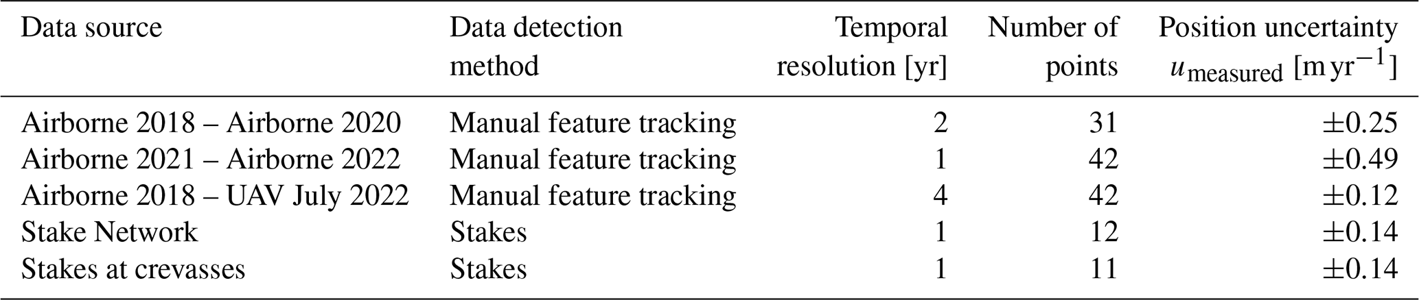
In order to provide a reliable ground-truth dataset of glacier surface velocities, identical features were tracked manually, using a combination of observations from UAV surveys and airborne imagery. Manual tracking allows the exclusion of features that are likely to have changed due to ablation, as described in detail in Appendix B. To minimize the impact by potential changes in ice dynamics over the recent years, the analysis was restricted to the period from 2018 through 2023, for which we assume that the ice dynamics did not change much. The data used for this period is summarized in Table 1. On VF, crevasses serve as the only reliable surface features for feature tracking, as no other distinctive surface forms are present. In order to reliably find the same feature in different data sets, only well-identifiable crevasse intersections are used. Because the crevasses are not equally distributed across the glacier, there are areas with sparse data coverage.

tiris Tirol (2025)Geissler et al. (2021)(Dobler, 2026)(Dobler et al., 2025)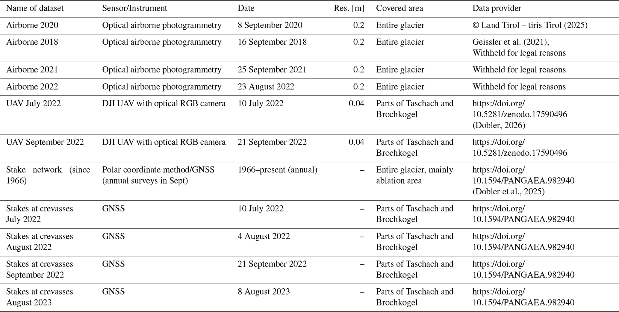

Table 1 Summary of available data showing ice dynamics of VF.

3.4 Compiled glacier velocity map

A map of recent velocities on VF has been generated by compiling manual feature tracking of crevasses and stake measurements for the period 2018–2023. To achieve a standardized temporal resolution, all measured displacements were converted to a mean annual velocity in meters per year. For displacement measurements taken during the summer months (July through September) or not on equal dates in the different years (e.g. from July 2022 to September 2023) a seasonal variation needs to be considered in the conversion factor. By comparing measured summer velocities at a few locations in the Brochkogel and Taschach area with the corresponding annual average, the seasonal variation is estimated to be approximately 30 % (detailed information see Sect. 4.2). Although the seasonal variation shows some differences between the Brochkogel and Taschach area and was only estimated for 2022/23, we consider the mean derived seasonality to be representative for the entire VF and assume its applicability to other years. Therefore, the seasonality observed in 2022/23 is applied to data covering the period from 2018 to 2023 where required. Additionally, a special set of features was created to comprise the glacier margin, where a movement of 0 m yr⁻¹ was assumed. Towards the margin, ice thickness decreases and consequently glacier dynamics slow down. Although a velocity of close to 0 m yr⁻¹ is very likely in these regions, it cannot be directly observed due to the lack of identifiable features. Therefore, specific points were defined to capture the marginal areas adequately.

In order to fill all data gaps and provide results with a uniform spatial resolution, the velocity data were interpolated onto a 50 m×50 m grid. Given the irregular data distribution and the presence of substantial gaps, natural neighbor interpolation was selected for its suitability in a geophysical context (Sambridge et al., 1995). Natural neighbor interpolation provides an effective balance between computational efficiency and result quality. As a localized method, it ensures that each interpolated point is only dependent on its immediate natural neighbors. A detailed explanation of the method is provided in Amidror (2002). The technique is implemented in MATLAB using the “scatteredInterpolant” function with the “natural” interpolation method.

As previously mentioned, a detailed mass balance study indicates that the Schwarzwandzunge area behaves fundamentally different from the rest of VF (Reinwarth and Escher-Vetter, 1999). Due to this differentiation and the scarcity of current velocity data, also from the Hochvernagt area, the compiled velocity map for the period 2018–2023 of this study focuses on the Taschach and Brochkogel areas. The study region for the velocity map is shown in Fig. 1.

3.5 Shallow-ice approximation method

The observed datasets of surface mass balance (SMB) and in-situ surface velocities motivate an investigation of the role of glacier geometry, as variations in SMB directly affect glacier geometry, which influences surface velocities. To assess whether the observed velocity trends can be reproduced by geometric changes, we apply a simplified shallow-ice approximation (SIA) method. This approach requires only the geometry, consisting of the surface slope (α) and the ice thickness (H), to estimate the velocity (e.g. Hutter, 1983; Greve and Blatter, 2009). The SIA approach is also referred to as a “zero-order” model, where only vertical shear stress gradients are taken into account. We therefore do not regard this as ice dynamic modeling in the strict sense, but rather a first approximation. The selected physical flow parameters are summarized in Table 2. The total surface velocity (u_total) consists of the deformation velocity (u_deform) and the basal sliding velocity (u_basal):

$$\begin{array}{}\text{(1)}& {\displaystyle }{\displaystyle }{u}_{\text{total}}=u_{\text{deform}}+u_{\text{basal}}\end{array}$$

Table 2 Parameters of the SIA model.

For calculating the deformation velocity soft and temperate ice was assumed by choosing a rheology parameter A corresponding to a temperature of 0 °C (Paterson, 1994). The deformation velocity is given by:

$$\begin{array}{}\text{(2)}& {\displaystyle }{\displaystyle }{u}_{\text{deform}}={\displaystyle \frac{\mathrm{2}A}{n+\mathrm{2}}}{\mathit{\tau }}^{n}H,\end{array}$$

where the shear stress τ is described as:

$$\begin{array}{}\text{(3)}& {\displaystyle }{\displaystyle }\mathit{\tau }=-\mathit{\rho }gH\sin \left(\mathit{\alpha }\right)\end{array}$$

The basal sliding velocity estimation requires a basal sliding coefficient C. As a priori determination is challenging, we tuned the coefficient so that the modeled velocity fall within the range of the measured velocities. The basal sliding velocity can be described as:

$$\begin{array}{}\text{(4)}& {\displaystyle }{\displaystyle }{u}_{\text{basal}}=C\cdot {\mathit{\tau }}^n\end{array}$$

In order to apply the SIA approach, annual ice thickness and surface slope are required. For this purpose, DEMs were generated by interpolation between available DEMs at known times (Finsterwalder, 1972; Rentsch, 1982 and more recent maps published by the group at BAdW) for workflow, see Fig. 2. All available datasets are listed in the Supplement.

Figure 2 Flowchart for calculating ice thickness and surface slope.

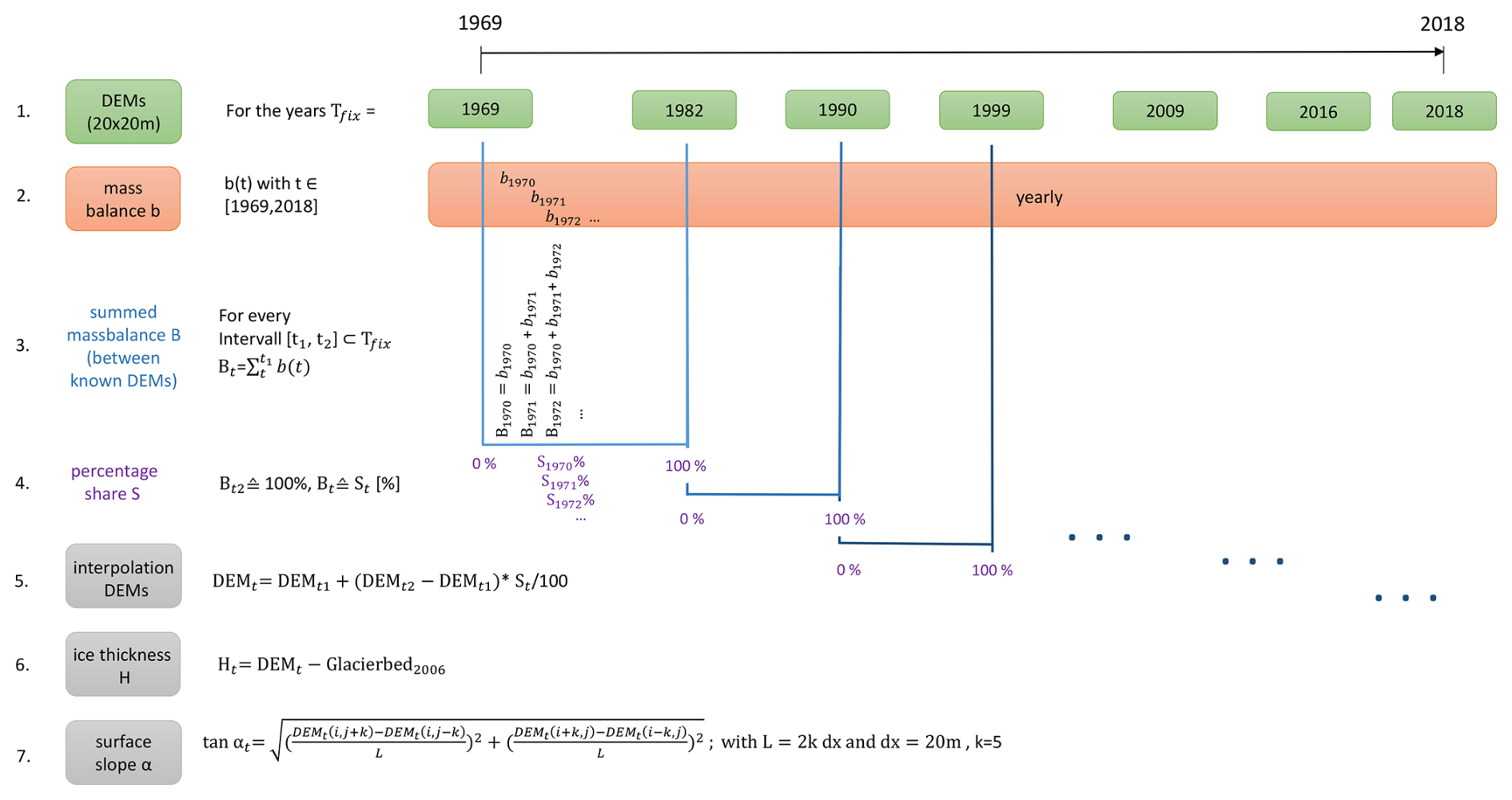
Instead of assuming linear interpolation over time, the interpolation between two consecutive DEMs was scaled according to the cumulative SMB. The annual mass balance is determined through the glaciological method and is described by a single glacier-wide value per year, as area distributed annual mass balances from the glaciological method are not available for all periods (WGMS, 2024). For example, the DEM from 1969 and 1982 is available, the years in-between are interpolated. Therefore, we started to sum the SMB during this period of time and used as relative measure of surface elevation change. This means, that the elevation change between the DEMs from 1969–1982 corresponds to 100 % of the cumulative SMB from 1969–1982 (in this example −596 mm w.e.). The yearly change in DEMs were generated according to the cumulative SMB reaching the respective year, for example cumulative SMB 1969–1976 with −520 mm w.e. corresponds to 87 %, meaning that 87 % of the elevation change from 1969–1982 would be applied to the DEM in 1976. In this way, elevation changes are distributed non-linearly in time and reflects periods of higher or lower loss/gain. The error of non-linear ice transport over time is neglected, as the velocities are relatively low. The respective ice thickness is derived by subtracting the bed topography of 2006 (Mayer et al., 2013b) from the corresponding interpolated DEM. Surface slope was calculated from the annual DEM using five grid cells (k=5) in each horizontal direction, with a grid size (dx) of 20 m, the baseline length (L) is 200 m. The resulting ice thickness and surface slope were restricted to the last known glacier extent. To compare the calculated velocity to in-situ stake observations, we extract the calculated velocity from the 20 m×20 m grids using a nearest-neighbor approach.

4 Results

4.1 Long-term ice dynamic

The examination of historical velocity data is essential to assess long-term trends and investigate the development of glacier dynamics. For this purpose, the stake network data, which has been measured annually at VF since 1966, is analyzed. Figure 3 displays the stake positions during the years. Since the focus lies on evaluating the temporal evolution of the ice movement, only time series of at least six consecutive years are considered. The data clearly demonstrate that stake displacements follow the flow structures of the different glacier tributaries. In addition, the generally decreasing distance between the annual stake positions of each data series indicates that stake velocities decrease over time. Figure 4 presents the annual velocity of six particularly long time series, highlighting a brief acceleration phase around 1980, followed by a pronounced and sustained decline. This velocity peak concurs with a period of positive mass balance, while the subsequent decline coincides with a sustained negative mass balance since 1980. This clearly illustrates the sensitivity of the ice movement to changes in surface mass balance.

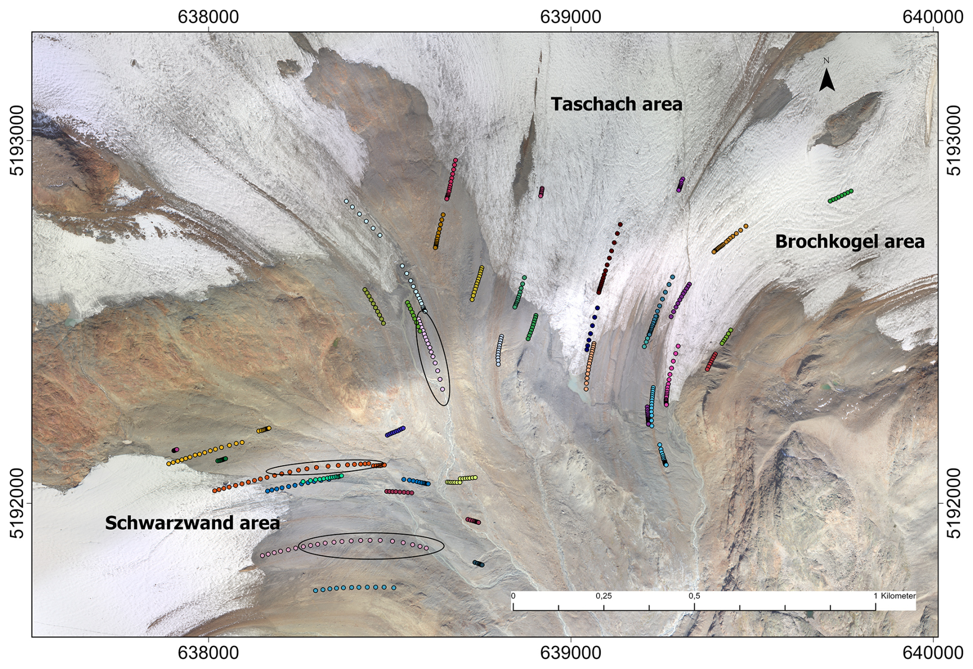
Figure 3 Annual position of the stakes measured for at least six subsequent years in the period 1966–2023. The colors indicate the same stake tracked over multiple years. The color coding correlates with Figs. 4 and 5. The black ellipses indicate flow paths that behave differently from the rest (see discussion in Sect. 5). Background image: Orthoimage 2016 © Bavarian Academy of Sciences and Humanities (BAdW), 2016.

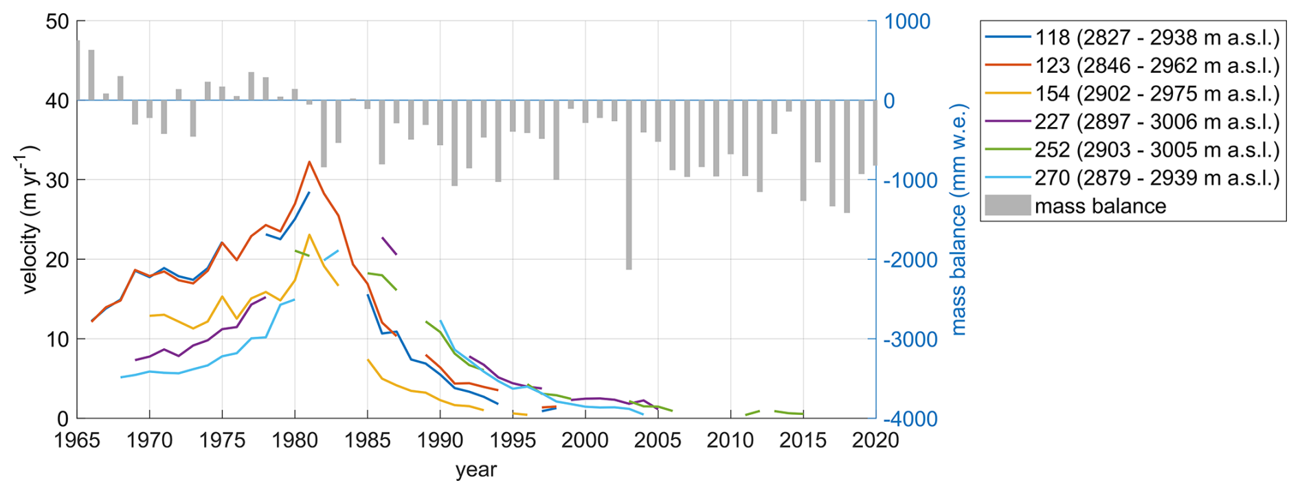
Figure 4 Annual stake velocity for particularly long time series and the corresponding annual glacier mass balance. The maximum elevation (earliest observations) and minimum elevation (most recent observations) of each stake are indicated in brackets to allow an assessment of its respective altitude.

To evaluate a possible reproduction of the velocity trends using only geometry, we compared the measured velocities with modeled velocities (from the SIA approximation) in Fig. 5. While the modeled values provide the same dynamic trends as the measured, offsets occur, which can be attributed to uncertainties in the input data (especially the ice thickness) and the temporally fixed choice of flow parameters. However, it is remarkable that even the small effect of slightly positive mass balance years on the glacier geometry, results in very pronounced changes of ice flow.

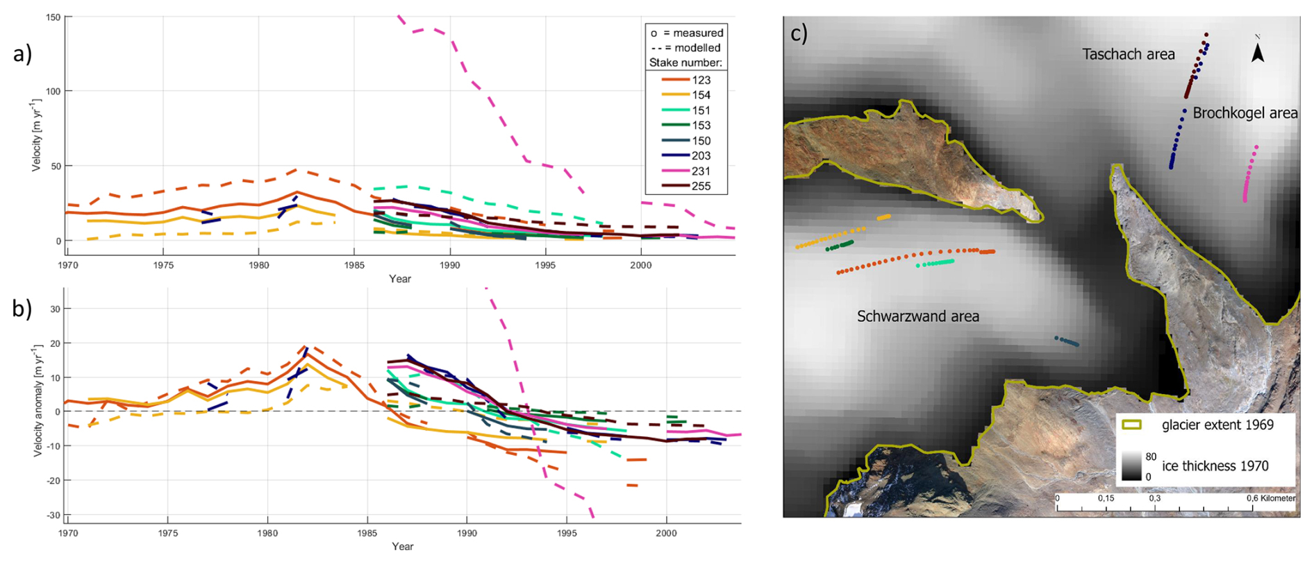
Figure 5 Measured and modeled stake velocity according to a shallow-ice approximation for selected stakes (a) as absolute values and (b) as anomalies from the long-term mean of each stake. (c) Position of the selected stakes with the glacier extent from 1969 and the ice thickness from 1970 (details on the calculation see Sect. 3.5). Background image: Orthoimage 2016 © Bavarian Academy of Sciences and Humanities (BAdW), 2016.

Over time, surface velocities at all altitudes decrease significantly (see Fig. 6). However, for altitudes exceeding 3000 $\mathrm{m}\mathrm{a}.\mathrm{s}.\mathrm{l}.$ in the previous years, this trend cannot be conclusively established due to insufficient data availability. In the range of 2900–3000 $\mathrm{m}\mathrm{a}.\mathrm{s}.\mathrm{l}.$ the reduction is most evident. In addition, Fig. 7 shows the regional distribution of surface velocities in connection with the respective ice thicknesses. Overall, a decrease in velocities can be observed at all altitudes, although their magnitude varies. The decrease in surface velocities is particularly pronounced at the Schwarzwand tongue between the periods a (1970–1980) and b (1990–2000). In contrast, the decline is less significant in the area of the Taschach tongue. These differences can be attributed to the interaction between ice dynamics and ice thickness. Between the two periods, the ice thickness reduction at Schwarzwand tongue is substantially greater, being approximately 35 %, whereas at Taschach tongue, the reduction was only about 10 %.

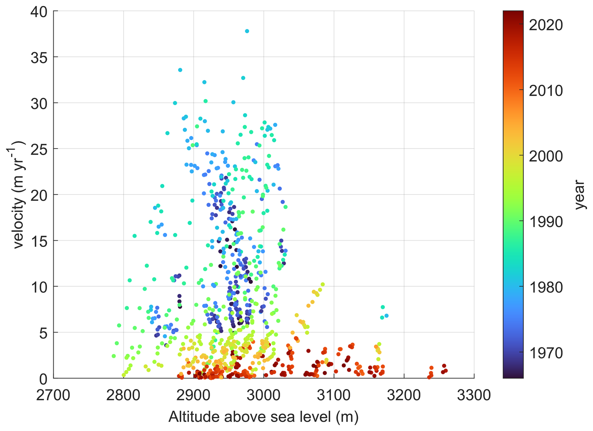
Figure 6 Glacier velocities of all observations in m yr⁻¹ in dependence of altitude and time (color code).

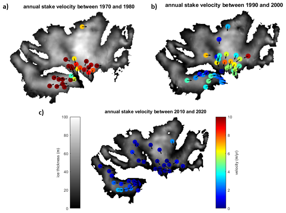
Figure 7 Mean annual stake velocities during the indicated period (a) between 1970–1980 with 1975 ice thickness (b) between 1990–2000 with 1995 ice thickness (c) between 2010–2020 with 2015 ice thickness. Details on the ice thickness calculation can be found in Sect. 3.5. The arrows indicate the determined flow direction, which is calculated from the mean angle of movement of the respective stake.

To quantify the ice dynamic process, we performed an analysis based on the observed geometry change, using surface elevation change derived from known DEMs (hereafter referred to as surface elevation change). Based on the ice thickness equation (Greve and Blatter, 2009), the dynamic contribution to ice thickness change can be computed by subtracting the local surface mass balance (SMB) from local changes in ice surface elevation. The residual component represent the local dynamic contribution to the vertical surface adjustment (assuming a stationary bedrock). The spatially distributed SMB for VF are available only from 1996 ongoing (earlier information as glacier-wide values). With a spatially distributed SMB and a surface elevation change map, the difference can be calculated as local dynamic contribution to elevation change.

We apply this analysis to the period 2016–2018, for which data availability is particularly good. Although this is a very short period with regards to glacier response times, it is assumed to be representative of the current ice dynamics, as the glacier already has very low velocities during this period, similar to those observed in 2018–2023. The cumulative SMB for the years 2017 and 2018, is shown in Fig. C1a, while the surface elevation change between the years 2018 and 2016 can be seen in Fig. C1b. The difference between the two maps provide the local dynamic contribution to elevation change (Fig. C1c).

In the accumulation areas (or former accumulation areas), negative values (red areas) indicate that the ice transport has a vertically downward component. In the ablation areas, on the other hand, positive values (green areas) indicate vertical mass compensation through ice transport. Figure C1c shows that the Taschach and Brochkogel areas exhibit hardly any vertical mass compensation (values very close to 0). In contrast, a local dynamic contribution to elevation change is still present in the former accumulation areas of these two sub-areas. The two green areas in the Taschach area provide good control. These are rock islands that were not excluded from the SMB map. However, the rock islands have remained stable during the period and have not moved, which is why they appear incorrectly as dynamic contribution to elevation change.

A closer look at the Schwarzwand area in Fig. C1c reveals a stronger dynamic contribution to elevation change. In the northern accumulation area of the Schwarzwand area (as well as on the Hochvernagt plateau), positive values are observed that cannot be plausibly attributed to a dynamic contribution to elevation change. It seems that a substantial accumulation area is missing. However, in the orthoimages, these areas are partially covered by snow and have hardly any features. It can therefore be assumed that the surface models in this area are uncertain. In addition, the SMB map (Fig. C1a) is largely interpolated (in particular in the northern part of Schwarzwand area), further increasing the uncertainty of the estimated dynamic contribution to elevation change in this region. It is also possible that these are formerly significant accumulation areas that are no longer very pronounced. Pronounced negative error values are present in the northern part of the Hochvernagt plateau (Fig. C1c). These originate from the surface elevation models, where an error has likely occurred.

In order to enable a numerical estimation of the processes, which excludes outliers as far as possible, the median of the absolute mass balance and the absolute dynamical contribution were calculated separately for the three glacier parts. The median of the absolute mass balance amounts to 1.48, 1.32, and 1.06 m yr⁻¹ for the Taschach, Schwarzwand and Brochkogel area, respectively. The corresponding median of the absolute dynamical contribution to elevation change are 0.54, 0.43, and 0.74 m yr⁻¹. For the mass balance determined by the glaciological method, a total uncertainty of less than 0.40 m yr⁻¹ can be assumed (Zemp et al., 2013). For the period 2016–2018, an uncertainty of approximately 0.28 m yr⁻¹ can therefore be calculated, taking into account the law of error propagation. The mean errors of the DEMs can be estimated at approximately 20 cm for 2016 and 10 cm for 2018 (tiris Tirol, 2025). Taking into account the law of error propagation, this results in an uncertainty of 0.11 m yr⁻¹ for the surface difference from 2018 to 2016. For the dynamic contribution to elevation change, calculated as the difference between SMB and surface difference, a total uncertainty of approximately 0.30 m yr⁻¹ can be assumed. Overall, further uncertainties must be taken into account, such as the compression and thus the change in altitude of possible firn areas due to a change in density, especially in the accumulation areas.

4.2 Seasonal variation

The measured values at different times (Fig. 8 and Table 3) clearly indicate that ice surface velocities are subject to seasonal variation. This is based on stake measurements in active moving terrain in the period 2022–2023, located in the Brockogel (4 stakes) and Taschach area (8 stakes). In the Brochkogel area, summer velocities are around 20 % (July–August) and 49 % (August–September) higher than the respective annual values. In the Taschach area, summer velocities exceed the corresponding annual mean by approximately 30 % (July–August) and 31 % (August–September). Thus, the seasonal variation averages 30 %. However, we consider the derived seasonality to be representative for the entire VF for July–September and assume its applicability to other years, although 2021/22 was a year with an extremely negative mass balance.

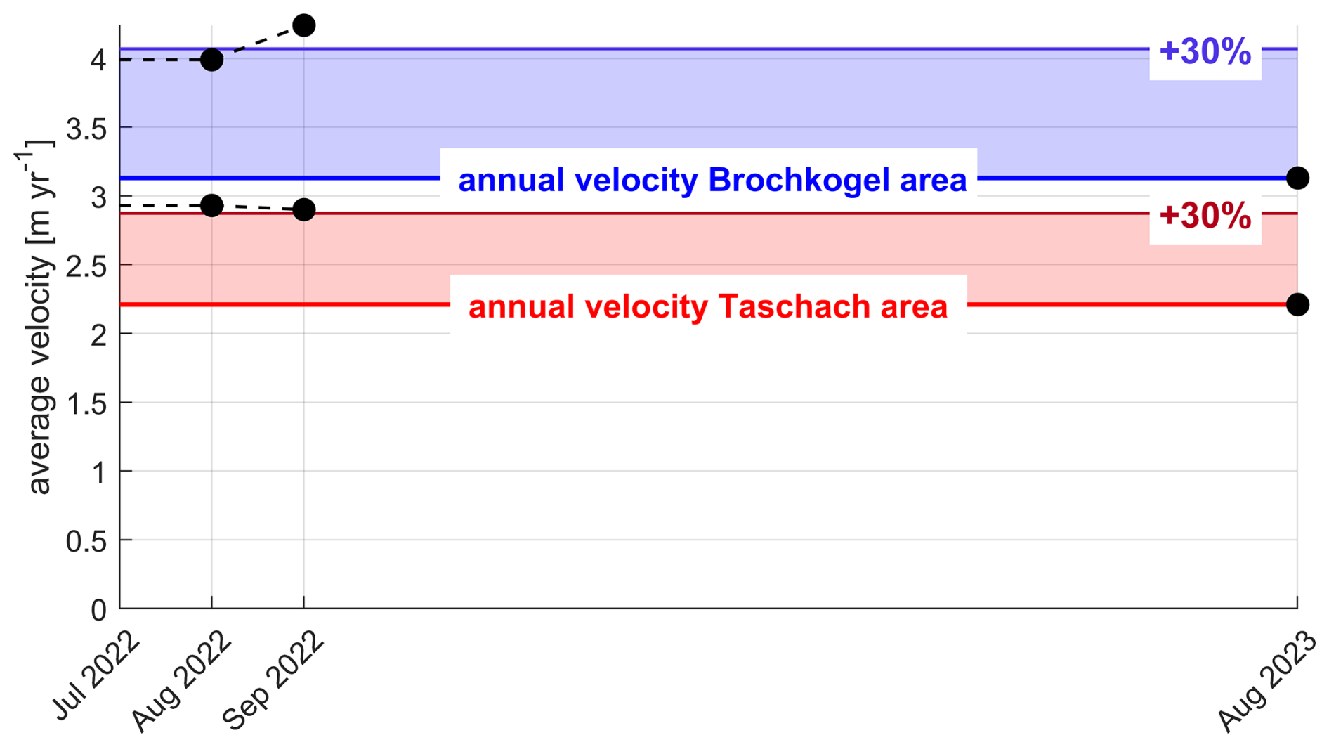
Figure 8 Seasonal variation of glacier surface velocity averaged over Taschach (8 stakes) and Brochkogel area (4 stakes).

Table 3 Values of summer (v_JA, v_AS) and annual surface velocity (v_a) and the calculated seasonal variation ($v_{\text{AS}}/v_{\mathrm{a}}$, $v_{\text{JA}}/v_{\mathrm{a}}$) for Taschach (8 stakes) and Brochkogel area (4 stakes). The uncertainties for the respective periods are: 22–23 August (365 d) ±0.14 m yr⁻¹, 22 July–22 August (25 d) ±2.06 m yr⁻¹, 22 August–22 September (48 d) ±1.08 m yr⁻¹.

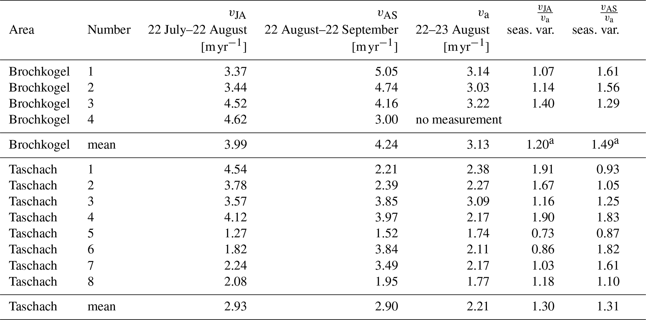
^a The mean ist without the measurement of Brochkogel 4.

4.3 Present day velocity

4.3.1 Standard satellite remote sensing measurements

Since user-ready products do not provide reliable results at VF (see Appendix A), we analyzed dedicated image pairs from higher resolution TerraSAR-X scenes. The microwave scenes also have the advantage of not being influenced by cloud cover. However, this dedicated analysis did not provide satisfactory results. For short temporal baselines (<100 d), the obtained displacement rates are unrealistically high (compared to the ground truth information from stake measurements, see Table 4). More realistic displacement rates are obtained for long temporal baselines. However, maximum velocities are located at the glacier tongue, which is also unreliable. Resulting example surface velocity fields from TerraSAR-X data analysis are provided in Fig. 9 for short and long temporal baselines. Furthermore, no results could be obtained from feature tracking of the high-resolution aerial imagery from subsequent years as the differences between the images did not allow the identification of unique features. Due to inconsistencies in the results from the standard satellite remote sensing data sets with feature tracking, they were excluded from further analysis.

Table 4 Overview of generated velocity points.

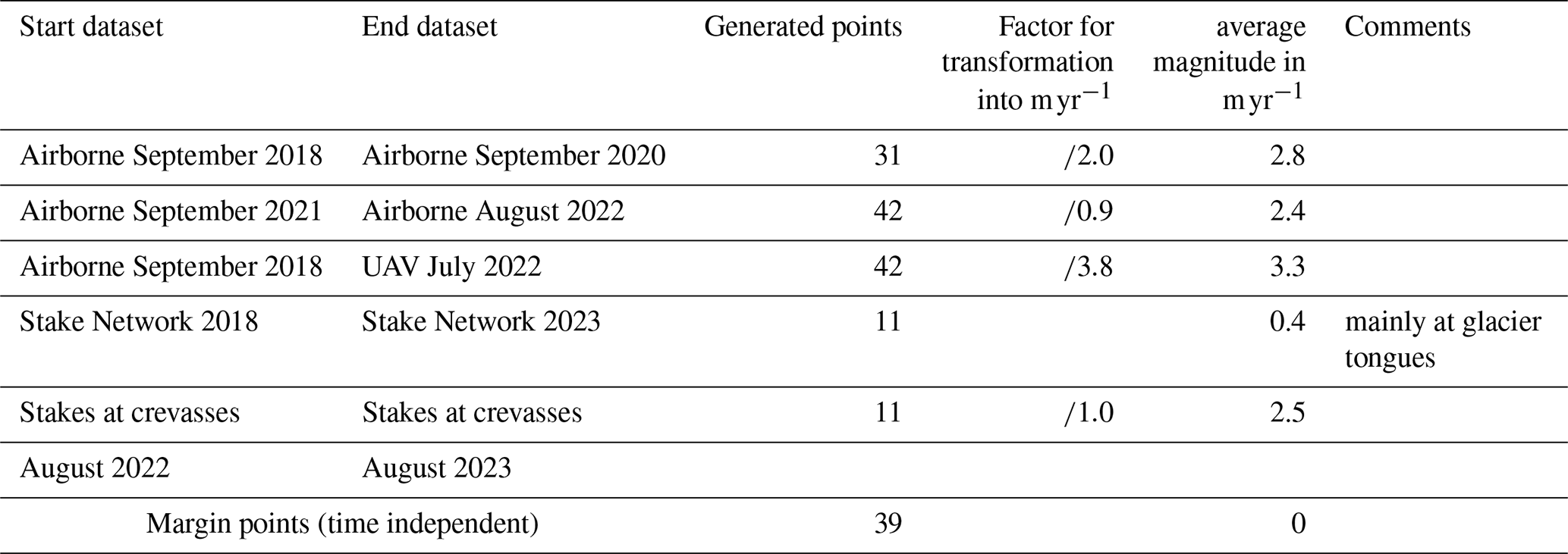
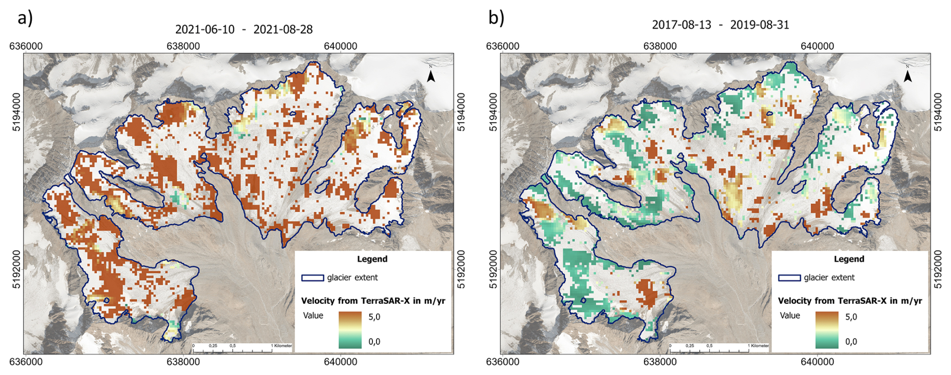
Figure 9 Magnitude of the surface velocity field derived from TerraSAR-X images (a) from 10 June 2021 and 28 August 2021 (temporal baseline: 83 d) and (b) from 13 August 2017 and 31 August 2019 (temporal baseline 748 d). Background image: Orthoimage © Land Tirol – tiris 2020.

4.3.2 Gridded velocity map for a glacier sub-region

Due to the combination of high ablation and slow velocity (for examples, see Appendix B) we decided to use manual feature tracking to produce a reliable surface velocity map from aerial or satellite imagery for the slow-flowing VF with maximum velocities of less than 5 m yr⁻¹. A sub-region with a high density of ground measurements was selected for obtaining a gridded representation of ice flow. For this purpose, we combined multiple datasets which results in 176 velocity points unevenly distributed over the sub-region of VF. Table 4 gives an overview of the datasets used and the detected features. However, the data set includes observations from different periods and thus the velocities are affected by seasonal variations. As previously mentioned, on VF it can be assumed that summer velocities are about 30 % higher than the annual average. This seasonal variation was taken into account when converting velocity data recorded at different times into meters per year. For transparency, the correction factor, which incorporates the seasonal variation, is also presented in Table 4. A natural neighbor interpolation of the compiled data set was performed and the resulting velocity map for the period 2018–2023 is presented in Fig. 10. The Figure shows the data points used and the corresponding flow directions. The data points are distributed unevenly, with a higher density in the active moving zones. The maximum velocities of 4 m yr⁻¹ also appear in these active moving zones, while the average surface velocity is about 1 m yr⁻¹. In the lower and margin areas, the surface velocity is slightly higher than 0 m yr⁻¹. In general, the ice flow direction follows the glacier slope.

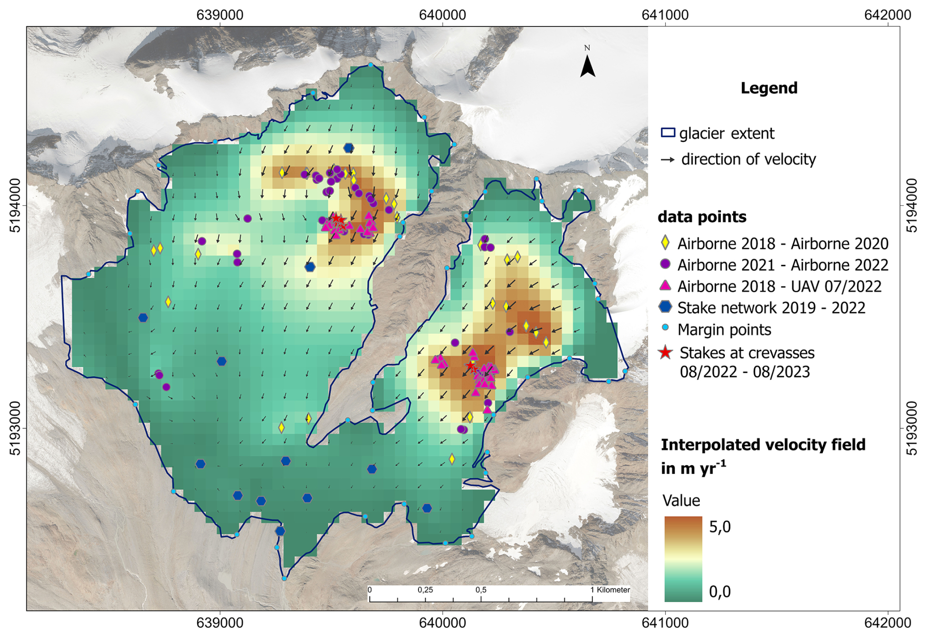
Figure 10 Map of mean surface velocity for the period 2018–2023 [m yr⁻¹], including the positions of the data points used for the interpolation, with different symbols indicating the data origin. Background image: Orthoimage © Land Tirol – tiris 2020.

4.4 Uncertainty Analysis

This chapter describes the results of the uncertainty analysis, details of the error calculation can be found in in Appendix D. The accuracy of all stake positions depends on the respective measurement method (multiple forward intersections, terrestrial polar coordinate method, and GNSS (Global Navigation Satellite System) positioning). In all cases, the placement of a prism or Antenna, depending on the method, requires a small horizontal offset due to the physical presence of the wooden stakes, which prevents exact alignment with the center of the borehole. Moreover, if the boreholes are not drilled vertically in the ice, melting can also cause further displacement biases. In combination with the measurement error, which is in the order of 3 cm, these factors result in an estimated general uncertainty of ±10 cm. Therefore, all positions in the stake data set, as well as in the figures of the multi-year stake displacements, are affected by this uncertainty. On average, seasonal variation is 1.30 (130 %), with a standard deviation across all observations of 0.37 (37 %). In addition to stake measurements, manually tracked surface features (e.g. crevasse intersections) were used to derive independent glacier surface velocities. The uncertainty of localizing these features depends on the image resolution (≤20 cm pixel size), the feature size (≥40 cm), possible sideways oblique views of the features (depending on the respective angle, in the order of around 5 cm) and the co-registration accuracy of the images. Considering these parameters, the feature position uncertainty can be estimated at ±35 cm. Manual case-by-case verification and explicit searching for crevasse intersection points ensure that only features with minimal change due to ablation are selected, thus guaranteeing this very high quality.

A covariance propagation law can be used to estimate the uncertainty of the calculated velocities, depending on the temporal resolution and the data detection method. The resulting velocity uncertainties represent one standard deviation (1σ) and are listed in Table 5, a detailed description to the calculation is in Appendix D. It is also demonstrated that an approximate total measurement uncertainty of 0.31 m yr⁻¹ can be estimated. For instance, feature tracking with a 2 year interval results in a velocity uncertainty of ±0.25 m yr⁻¹, whereas a 1 year interval yields ±0.49 m yr⁻¹.

Table 5 Statistics of all points used for the interpolated velocity map. The reported uncertainties represent one standard deviation (1σ).

The natural neighbor interpolation of all observations listed in Table 5 yields a correlation coefficient (R) of 0.94 for eastward velocity and 0.95 for northward velocity. The residual variance is 0.15 m, respectively, which indicates a robust and consistent representation of glacier flow. To examine the uncertainty of the interpolation more closely, a leave-one-out method was performed (e.g. Grab et al., 2021. This shows that there is no significant dependence of the misfit (between interpolated velocity and measured velocity) and the distance to the next observation. However, a relative interpolation uncertainty of 57 % and an absolute interpolation uncertainty of 0.8 m yr⁻¹ can be estimated from the standard deviation. Detailed calculations and explanations can be found in Appendix D. The reliability of the interpolated map is further supported by the overall alignment of the calculated flow directions with the glacier topography (slope direction), with no significant outliers observed. The median angle deviation is 43°, but larger deviations may occur at very low magnitudes. Despite the estimated interpolation error, the velocity map becomes less reliable in regions with limited data availability. In zones where observational data is lacking, there is insufficient information, making the reliability of the velocity map for understanding ice flow dynamics in these areas questionable. For the period 2018–2023, annual surface velocities are assumed to be constant. This assumption is supported by stake measurements, which show a maximum year to year variation (decrease) of 10 % within measurement uncertainty. We therefore assume that there is no significant change during this period.

5 Discussion

5.1 Ice dynamics

This subsection discusses the observed changes in glacier flow. Long-term and seasonal variations are interpreted in relation to changes in ice thickness and mass balance. When examining historical data, a general decrease in glacier velocity over time is prominent. This trend can be attributed to two main factors. First, the stakes slow down as they approach the glacier tongue, in line with the general velocity decrease towards the tongue. Second, the reduction in ice thickness due to the continuous negative glacier mass balances influences the velocities, as deformation rates are directly dependent on ice thickness. Driving stress is directly related to ice thickness and thus a reduction in ice thickness leads to lower driving stress and therefore to a reduction in deformation rate. On VF the magnitude of velocity change varies depending on the region. This can be seen particularly at Schwarzwand tongue, where both the ice thickness and the velocities decrease significantly, even more than on the rest of VF. As ice thickness decreases, deformation rates and velocities decline, a well-documented pattern in glaciological studies. One exception to the general slowdown is evident, as marked by three black circles in Fig. 3. These cases show a temporary increase in velocity during the period 1975–1985. The accelerated ice flow during this period likely originated from the temporarily positive mass balances and an accompanying small glacier advance around 1980 (Mayer et al., 2013b). Neighboring glaciers, such as Hintereisferner show a similar velocity peak around 1980, followed by a decrease (Stocker-Waldhuber et al., 2019). The peak aligns with a wider regional trend, as a significant proportion of glaciers in the European Alps experienced advances during this temporarily relatively cool phase (Patzelt, 1985; Wood, 1988). We have found evidence that the displacement of ablation stakes at VF react quickly to a change in the mass balance. An ongoing period of predominantly negative mass balance starting in the early 1980s marks the onset of a decrease in surface velocity in the ablation area. Ice thicknesses are rather small in the tongue areas of VF, where the stake measurements are carried out. Ice velocity is very sensitive to changes in ice thickness and the relative change of ice thickness due to strong ablation. With already reduced dynamic compensation leads to a fast reduction in ice velocity. In a year with a strongly negative mass balance, the strong melt in the ablation area directly decreases ice thickness, which represents the current status of the glacier. Stocker-Waldhuber et al. (2019) have also found evidence that ablation stakes can be well suited to reflecting the current status of a glacier. They show that the Kesselwandferner (also in the Ötztal valley) shows relatively direct response of ablation area ice dynamics to changes in mass balance, regardless of the geometry of the glacier. On VF, there is insufficient data to substantiate this adequately. Further studies (including in other areas) are necessary to investigate this effect in more detail. Comparable behavior has been reported from long-term observations of the d'Argentière glacier, Mont Blanc area. Vincent et al. (2009) show an ongoing negative net mass balance since 1982, with a direct reflection (delayed by a maximum of 3 years) in the velocity. They describe that the change in velocities in the upper part of the glacier is smaller than in the lower part (ablation area). The velocity trend thus fits the VF timeline quite well.

A quantitative analysis of recent geometry change (period 2016–2018) at VF indicates that SMB is the dominant control, while local dynamic contribution to elevation change remains secondary. When interpreting the contributions of SMB and local dynamic contribution to elevation change, various uncertainties must be taken into account. For the investigated period (2016–2018), measurement uncertainties arise from SMB estimation (0.28 m yr⁻¹), DEM differencing (0.11 m yr⁻¹) and the derived local dynamic contribution to elevation change (0.30 m yr⁻¹). In addition to these measurement uncertainties, various physical processes may influence the observed elevation changes. For example, snow cover in the accumulation area can affect the DEM accuracy, while small local wind-driven snow transport events can modify the accumulation pattern and thus SMB. Additionally, avalanches and debris covered parts of the glacier may contribute to elevation change or altered ablation, although their overall impact at VF is assumed to be limited. These processes are not considered in the applied approach and may therefore lead to additional variations in the estimated local dynamic contribution to elevation change, particularly on small spatial scales. Despite these uncertainties, the significantly higher magnitude of SMB remains the dominant control on recent elevation change. The median absolute values for SMB (Taschach: 1.48 m yr⁻¹, Schwarzwand: 1.32 m yr⁻¹ and Brochkogel area 1.06 m yr⁻¹) and the local dynamic contribution to elevation change (Taschach: 0.54 m yr⁻¹, Schwarzwand: 0.43 m yr⁻¹ and Brochkogel area: 0.74 m yr⁻¹) suggest that the ice dynamic is not able to fully compensate the losses due to melt, especially in the ablation area. There are indications that there may be slightly more compensation of elevation change through ice dynamics in the Schwarzwand area and that this area behaves fundamentally different from the rest of VF. This was already suggested by Reinwarth and Escher-Vetter (1999) and can be confirmed here. Figure 7 also suggests a higher dynamic on the Schwarzwand tongue compared to the other tongues. Due to a lack of data (no spatially distributed SMB before 1996), it is not possible to quantitatively assess these processes for the early years of glacier observation. However, it can be assumed that the local ice dynamic contribution to elevation change was more pronounced during this time, as the measured velocities were significantly higher, particularly around 1980, with an absolute SMB being significantly smaller than it is today.

Short-term seasonal variations play a role in the general glacier flow behavior. A significant temporal variability is observed, with a notable difference between the summer and winter seasons. There is general agreement that this variability is influenced by the glacier size, as well as internal and subglacial hydrology, although this has not been clarified conclusively and is still a subject of current research (Vincent and Moreau, 2016; Sanders et al., 2018; Nanni et al., 2023; Troilo et al., 2024). In general, the seasonal variability can be rather large, with summer velocities either comparable or even up to 300 % higher than winter values (Nanni et al., 2023; Troilo et al., 2024). At VF, summer velocities are approximately 30 % higher than the annual mean, with a standard deviation across all observations of 37 %. The relatively high uncertainty results from the fact that the absolute measured values over a month (July–August or August–September) have maximum values of about 50 cm. However, these values have a relatively high measurement uncertainty of ±14 cm. Our measurements were conducted in summer 2022 in an area of higher ice flow, which is relatively high-elevated, but it is still not part of the accumulation zone and is strongly affected by melting. Meltwater input and the related increase in subglacial water pressure can reinforce the basal sliding of the glacier during the summer until an efficient drainage system is developed (Iken and Bindschadler, 1986). Crevasses and moulins can encourage the meltwater input to the glacier bed, increasing the basal sliding (Das et al., 2008). At our measurement area, such an increase in meltwater input can occur by existing crevasses, potentially also from upstream regions. As a result, seasonal variation may be stronger in our measurement area, particularly as efficient drainage systems are probably only well developed further down on the glacier tongue. Whether this summer velocity increase is representative for larger areas of VF and for other years has yet to be demonstrated. No assessment can be made regarding the time of highest seasonality because of the lack of measurement data, other studies refer to spring (Iken and Bindschadler, 1986; Bartholomaus et al., 2008), due to high melting rates combined with a not yet developed drainage system.

5.2 Implications for observations of glacier velocities

This part outlines the current challenges posed by very low ice velocities in combination with pronounced surface ablation. The annual surface velocities at VF are on average around 1 m yr⁻¹ while maximum velocities reach around 4 m yr⁻¹. These low velocities, in combination with strong surface ablation, pose a challenge for measuring the glacier flow using remote-sensing techniques like feature tracking. A sufficient displacement of the features between the consecutive acquisitions is needed. The retreat dataset is based on consecutive Sentinel-1 SAR acquisitions with minimum temporal baselines ranging between 6–48 d, depending on the region, and a maximum of 96 d (Friedl et al., 2021). For the Alps, a minimum temporal baseline of 48 d was employed. However, considering a spatial resolution of Sentinel-1 IW data of 10 m, the displacement rate at VF would correspond to 0.025 pixels for 96 d between the data takes, which is too small to be accurately captured by feature tracking. Typically, upsampling rates of 2–8 are employed to obtain sub-pixel displacement rates. However, the displacement rates at VF are too low, even for high-resolution TerraSAR-X stripmap data (2 m resolution). Moreover, the accumulation area has decreased significantly in recent decades, leading to widespread surface melting across large parts of the glacier (WGMS, 2024). The magnitude of point mass balance due to melting exceeds horizontal velocities in many areas on VF, meaning that observed feature velocity is heavily overlaid by surface changes caused by melting in summers, further limiting the unambiguous identification of features between the consecutive acquisitions. Interferometric techniques, such as SAR coherence tracking or InSAR displacement measurements, are hampered as well by the strong ablation rates during summers and snowfall throughout winters. These climatic factors also explain the observed limitations in the tacking results when using long temporal baselines, as tested for the TerraSAR-X data and selected ITS_LIVE image pair velocity fields. Moreover, the limitations in the individual image pair results can not be compensated by combining multiple results in monthly or yearly mosaics, since all output is affected by the various issues (see Figs. A1 and 9 and Sect. 4.3.1). Overall, the limited displacement rates, high surface melt during summers plus high accumulation during winter as well as the irregular distribution of surface features impede the capturing of the ice flow at VF by standard remote-sensing techniques. For other relatively slow-flowing glaciers, such as the Griesglacier, surface velocities could be derived over short time periods using UAV-based imagery and software such as IDMatch, a tool for automated velocity derivation (Gindraux, 2019). Compared to the VF, the average velocities on Griesglacier with more than 1 m in just 1 month are significantly higher than the average velocities at the VF of about 1 m yr⁻¹. Furthermore, a short test of the IDMatch software using the UAV VF datasets from July 2022 and September 2022 results in no correlation between the images. Regardless of the software and the potential detection of identical features, surface changes caused by strong ablation at VF remain a dominant source of uncertainty, as illustrated in Appendix B. We do not want to rule out the possibility of automated derivation, but it would be essential to additionally correct for the false values caused by the ablation-induced change in features (a change not caused by ice flow). For this reason, we have chosen manual feature tracking.

Our work reveals that standard remote-sensing velocity products, including those evaluated in this study, have limitations when applied to a slow-flowing glacier with pronounced surface ablation. Due to these limitations, ground-truth measurements and/or manual feature tracking can be the method of choice, although the methods are very demanding compared to standard remote sensing techniques. The manual feature tracking enables a focused segmentation of high-quality points, a task that remains challenging even to the human eye due to the significant surface changes over time (see Appendix B). It allows simultaneous plausibility checks of individual points, ensuring greater reliability.

Although we were not able to generate a surface velocity map for the entire VF, we successfully constructed a valid map of current velocity of the Taschach and Brochkogel area, demonstrating key dynamical mechanisms operating on the glacier. The map integrates multiple datasets for the period 2018–2023, primarily stake measurements and manually tracked crevasse features. Consequently, areas with many crevasses are represented by numerous data points, whereas regions lacking distinct surface features are sparsely covered, where stake measurements remain the only basis for the interpolated velocity map. A clear correlation is evident between the appearance of crevasses, indicated by areas with a high density of data points, and high velocities, up to 4 m yr⁻¹. A connection of crevasses and velocities is well-documented in the literature, including detailed studies such as Vaughan (1993). The assumption of zero velocity at the glacier margin when generating the velocity map neglects possible transverse stress couplings. Nevertheless, the dynamics at the margin of the glacier are significantly slower than in the center. Since the VF itself flows relatively slowly even in the center, the velocities at the margin will be close to 0 m yr⁻¹.

6 Conclusions

Long-term ice dynamic observations, recorded since 1966, reveal insights into the evolution of glacier dynamics under changing climatic conditions. A minor glacier advance around 1980 corresponds to a time of positive mass balance. As a consequence, there was a noticeable increase in velocity for a short period. A long series of negative mass balances during the subsequent years resulted in a significant decline in the surface velocities. Long-term observations at Vernagtferner indicate that glacier flow responds to changes in surface mass balance on short timescales, with velocity changes in the ablation area occurring within at most a few years. Recent ground-truth measurements enable the estimation of current seasonal variations in ice flow, with summer velocities being up to 30 % higher than the annual average. The estimation of surface velocities turned out to be challenging for slow-moving glaciers. With the general tendency of strong negative mass balances and the associated high ablation, changes in surface features may be caused predominantly by ablation rather than ice dynamics. In order to obtain detailed velocity information for the years 2018–2023, a velocity map was created manually using a combination of stake measurements and feature identification from UAV surveys and airborne imagery (excluding feature changes due to ablation as far as possible). With the general tendency of strong negative mass balances and the related slowdown, it will become increasingly difficult to determine surface velocities and thus ice flow on numerous glaciers across the Alps. Here, we highlight the challenges in deriving velocity information for such glaciers and demonstrate the value of long-term observations for investigating the change in ice dynamics due to continuous reduction in ice thickness. The results are a useful starting point for understanding the behavior of slow-flowing alpine glaciers and their variability in response to changing environmental conditions. The generated velocity map (available at Dobler et al., 2025) allow a detailed modeling of glaciological processes as well as plausibility assessments of future remote sensing results, but is only valid for the observed period (2018–2023), with the highest uncertainty in the regions with low data coverage. Overall, the mean uncertainty of all observations can be estimated at ±0.23 m yr⁻¹, with no outliers included. This indicates a high degree of reliability and thus provides a solid reflection of the glacier flow. However, a continuation of long-term in situ observation is essential for a better understanding of glacier dynamics and their response to climate change.

Appendix A: Review of existing products

There are user-ready glacier surface velocity products from NASA's ITS_LIVE (Gardner et al., 2022), FAU's glacierportal (Friedl et al., 2021) or a dataset published by Millan et al. (2022) for almost all glacier regions worldwide. Figure A1 exemplarily shows the ITS_LIVE velocities (for the period 2017–2018) and the Millan mosaic (for 2018) for VF. The results are based on feature tracking algorithms applied to Sentinel-1 Synthetic Aperture Radar (SAR) acquisitions, as well as optical imagery from Sentinel-2 and Landsat missions. The products are based on imagery with spatial resolutions of 10–30 m and provide results at 50–200 m spatial resolution. The accuracy of the products can vary strongly locally and depends on the velocity level, coherence, existing features, etc., but can be estimated at 0.08 m per day for a temporal baseline of 12 d (Gardner et al., 2022; Friedl et al., 2021; Millan et al., 2022).

The accuracy is insufficient for a slow-moving glacier such as the VF, as the speed is lower than the uncertainty of the measurement. This is the case for many slow-flowing glaciers, which are contained in the datasets and are already used in regional-scale modeling studies (e.g. Cook et al., 2023). We analyzed the mosaics, which show high spatial coverage and some kind of displacement signal on the glacier surface. However, a closer inspection of the displacement rates and in particular the directions showed that the displacements are very noisy and that the displacement directions are not aligned with glacier flow directions.

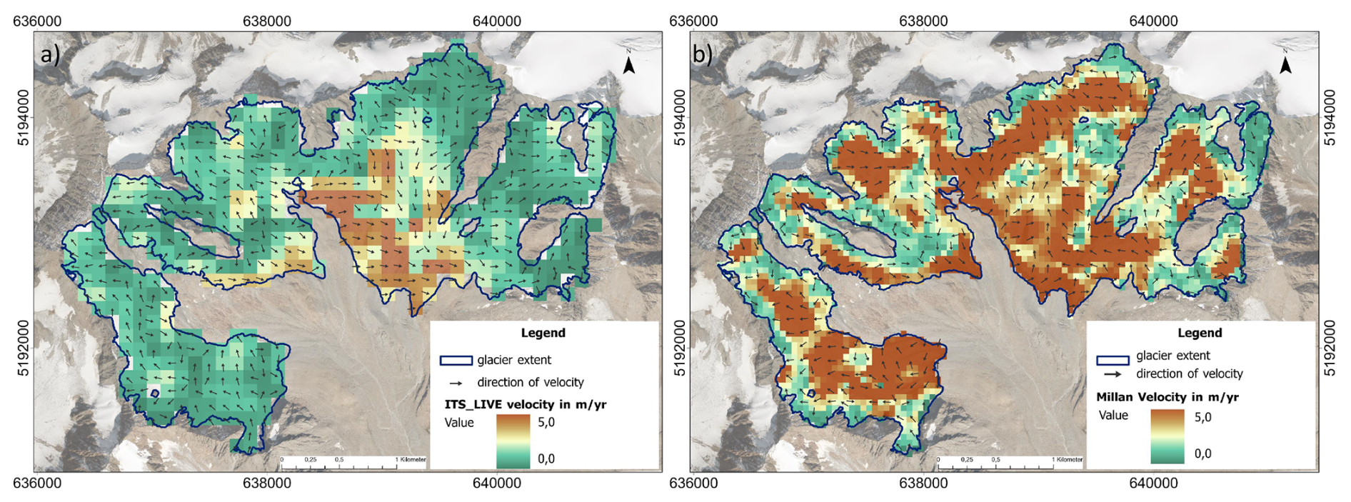
Figure A1 Annual surface velocity mosaic from (a) ITS_LIVE database for the period 2017–2018 (Gardner et al., 2022) and (b) Millan database for 2018 (Millan et al., 2022) using the same color scale. Background image: Orthoimage © Land Tirol – tiris 2020.

Appendix B: Melt-induced changes and manual feature tracking

The figures show the same situation at different points in time:

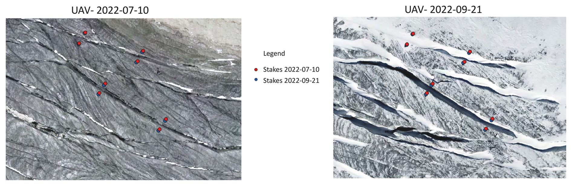
Figure B1 Melt-induced changes to crevasses. The example is taken from the upper part of the Taschach area at an altitude of approx. 3150 m. Maximum velocities occur in this area at the VF.

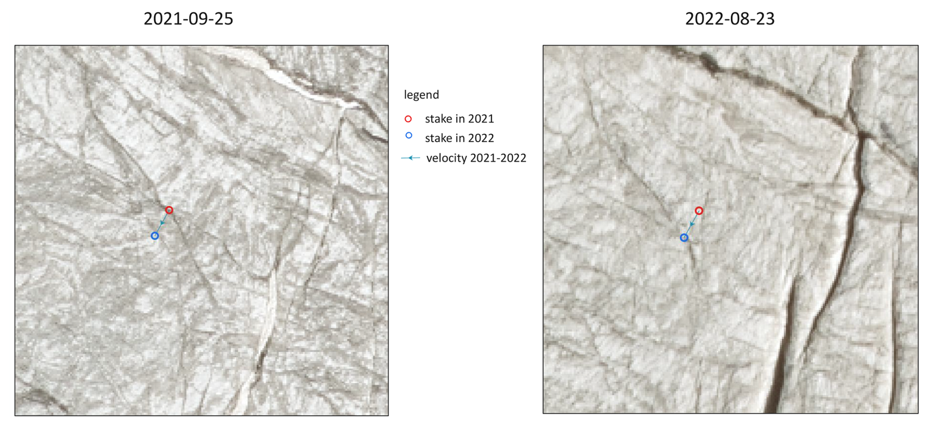
Figure B2 Melt-induced changes to crevasses. Example from the upper part of the Brochkogel area at an altitude of about 3200 m.

Figure B1 clearly shows a change in surface features, in particular a widening of the crevasses. We examined two of the crevasses in more detail using two stakes at the upper and lower edges of each crevasse. The average movement of the eight stakes (shown in Fig. B1) over the two months is approximately 0.73 m (change from the red to the blue points), with a standard deviation across the eight stakes of 0.12 m. The stakes rule out the possibility that a significant actual break-up of the crevasses has taken place. The stakes show an even shift of the upper and lower edges of the crevasses. Thus, the change in the surface features is probably largely due to melting. Even if identical features (in this case, crevasse edges) could be identified during the period, the movement would be significantly overlaid by ablation due to the crevasse edges (and their varying melt rates), resulting in erroneous dynamics.

Even with larger temporal baselines, manual feature tracking can be used to exclude features that are likely to have changed due to ablation, as is often the case in 2022. Crevasse trace intersections are particularly well suited for this purpose, as can be seen in Fig. B2. Identifying identical features that have not been subject to high ablation is challenging even for the human eye, especially over longer baselines, such as the example in Fig. B3 over a period of two years.

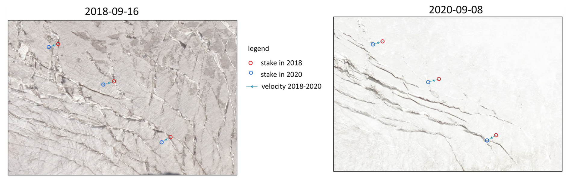
Figure B3 Crevasse pattern in a period without significant melt. Example from the highest part of the Brochkogel area at an altitude of about 3250 m.

Appendix C: Ice dynamics

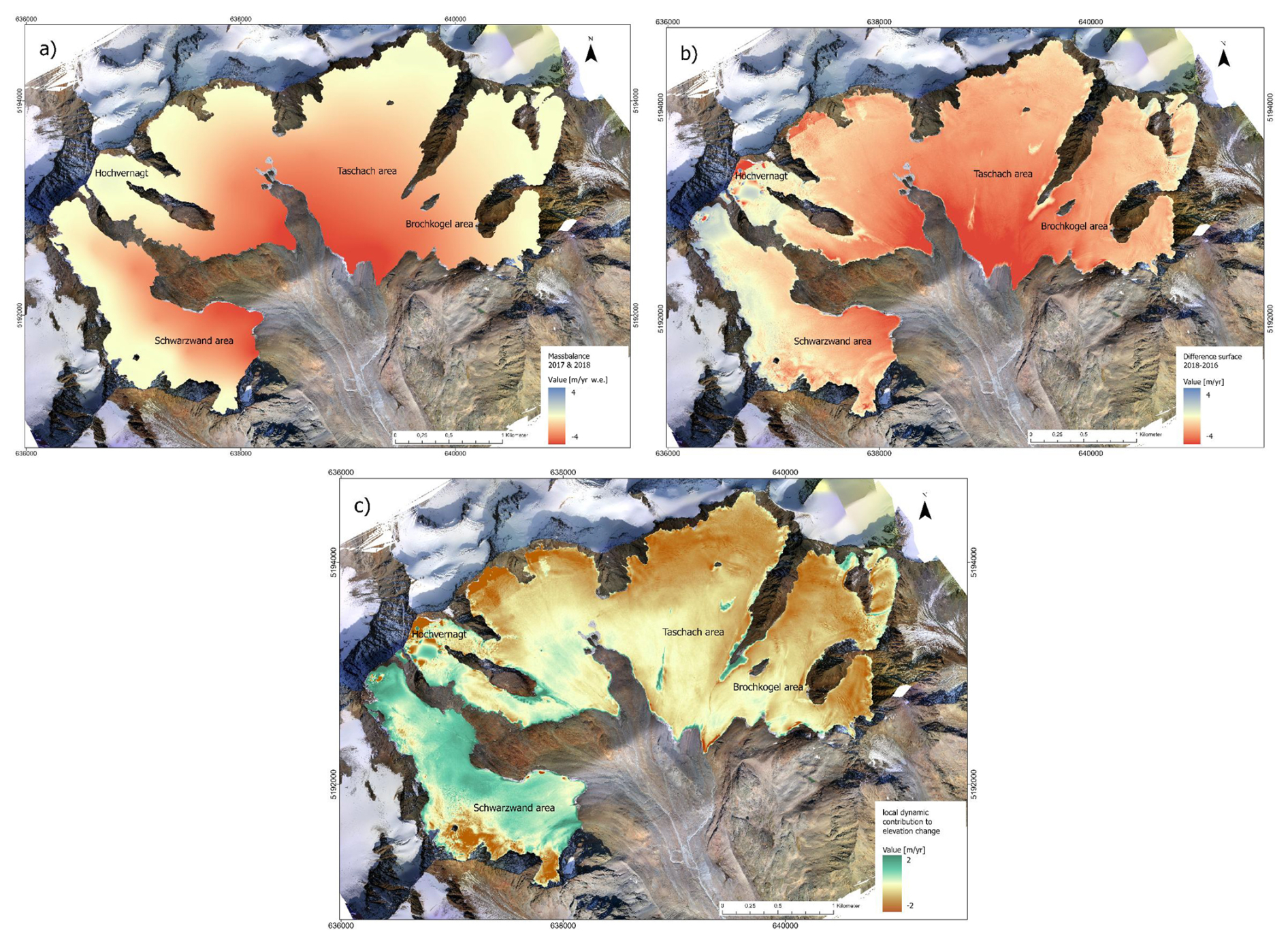
Figure C1 (a) areal distributed surface mass balance summed for the years 2017 and 2018, (b) surface elevation difference 2018–2016, (c) Difference between (a) and (b), which illustrates the local dynamic contribution to elevation change. Background image: Orthoimage 2016 © Bavarian Academy of Sciences and Humanities (BAdW), 2016.

Appendix D: Uncertainty

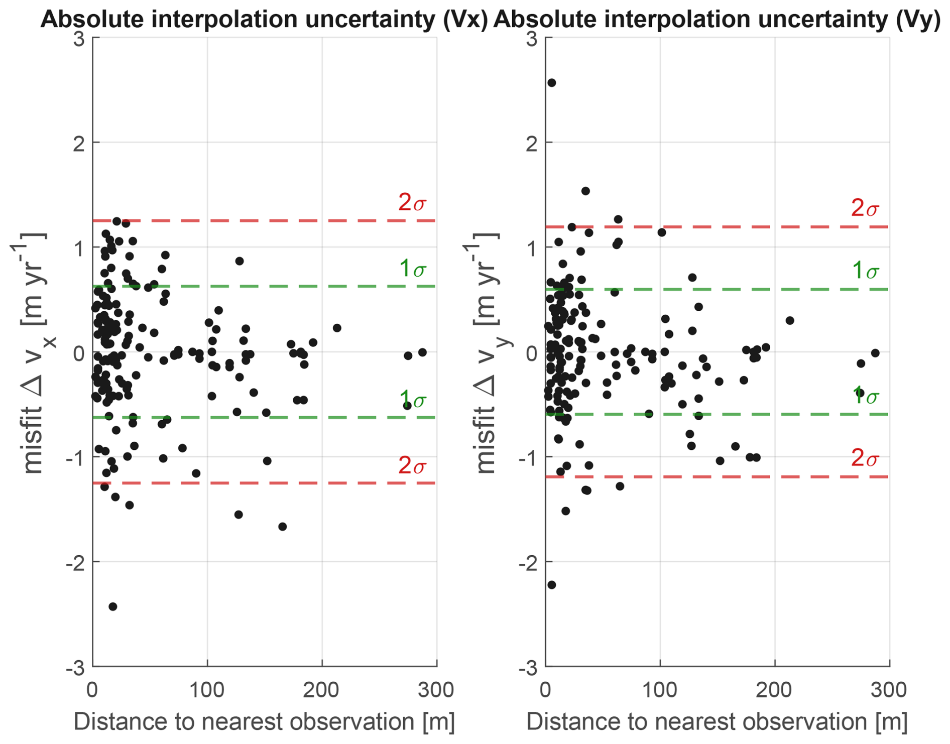
Figure D1 Misfit between interpolated and measured velocity (△v) vs. distance to the nearest observation according to a leave-one-out-method, referred to as u_{interpolation x} and u_{interpolation y}.

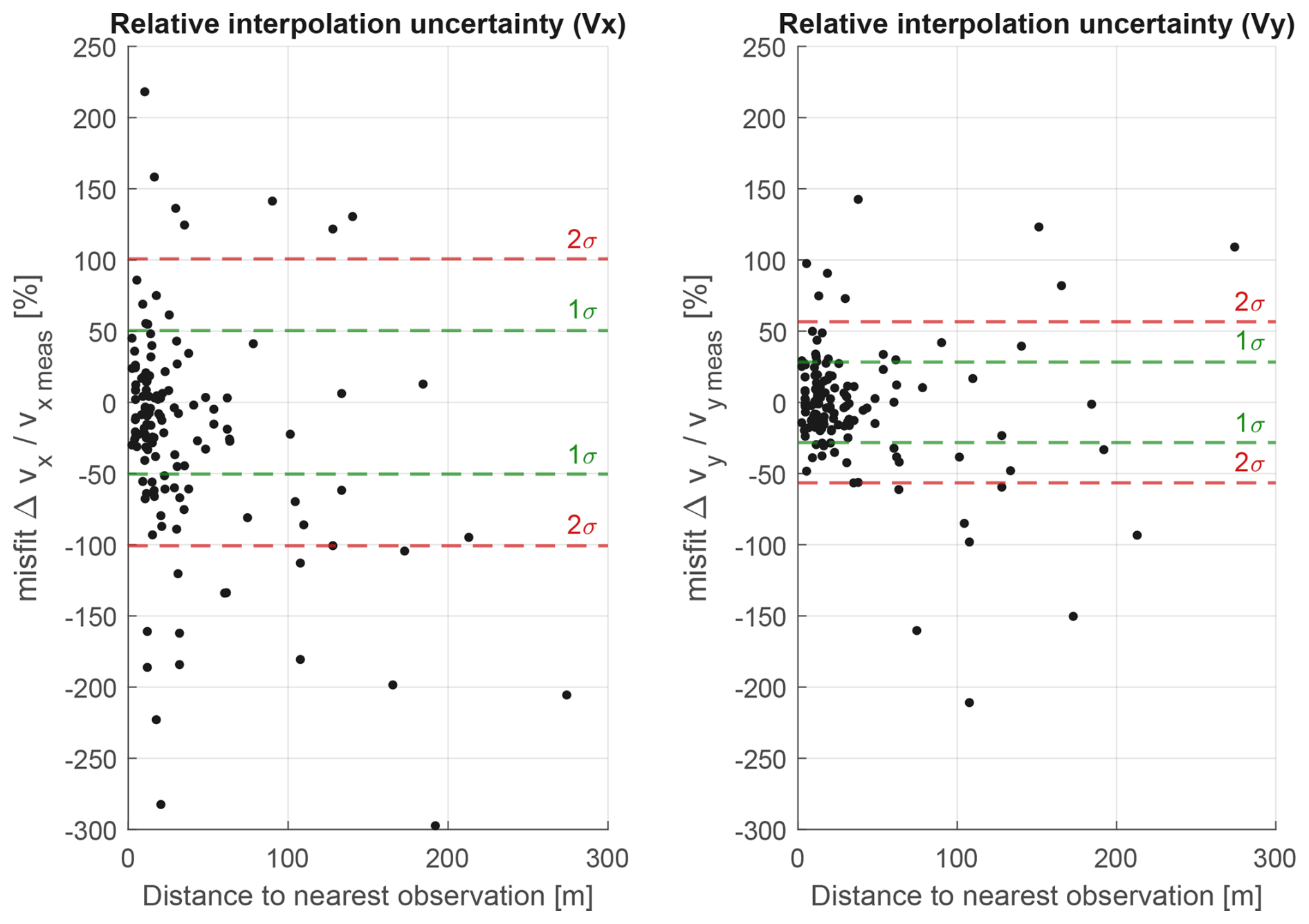
Figure D2 Misfit between interpolated and measured velocity (△v) in relation to the measured velocity (v_meas) vs. distance to the nearest observation according to a leave-one-out-method, referred to as u_{interpolation x} and u_{interpolation y}.

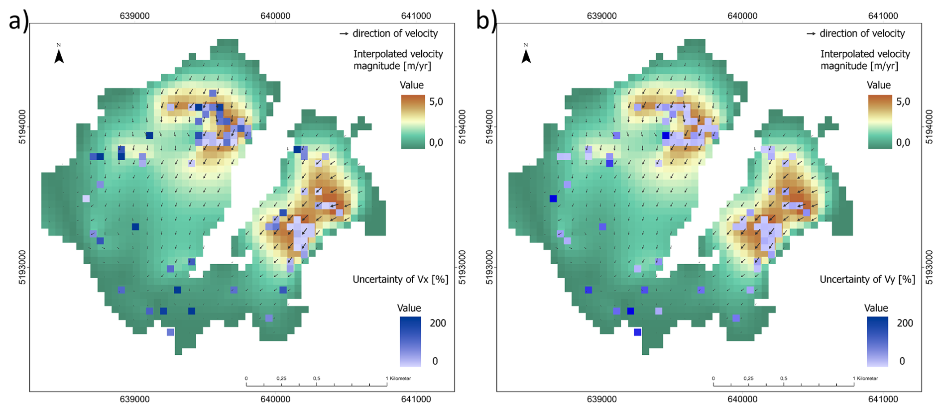
Figure D3 Interpolation uncertainty (u_{interpolation x},u_{interpolation y}) as misfit of a leave-one-out-method, with the misfit between interpolated and measured velocity (△v) in relation to the measured velocity (v_meas) for measuring points, averaged in case of overlaps. (a) for velocity in x direction, (b) for velocity in y direction.

A further uncertainty analysis can be performed using a leave-one-out method. For this purpose, an interpolation was performed for each point without using this point and the misfit of the interpolated velocity to the measured velocity was determined. The generated misfits are shown as relative and absolute errors with respect to the distance to the closest observation in Figs. D2 and D1. The figures show that there is no significant correlation between the misfit and the distance to the nearest observation. This is most likely due to the inhomogeneous distribution of points and the fact that there is a high point density with a high variation in magnitude in the crevassed areas, whereas there is a low variation with a low point density on the glacier tongue. This can be seen in Fig. D3. The individual misfits for each point are shown, with the mean average being formed in case of an overlay. The percentage uncertainty does not appear to be significant in specific areas. Due to the structure of the data, no statement can be made about a possible dependence of the interpolation uncertainty on the distance to the nearest observation point. Instead, as can be seen in Figs. D2 and D1, there is a normal distribution around the value 0, so a 1σ-confidence interval can be derived as the mean uncertainty of the interpolation (in x and y direction). The relative error is estimated at 50.4 % in x direction and 28.3 % in y direction, while the absolute error is 0.6 m yr⁻¹in each direction.

The interpolation uncertainty (u_{interpolation}) for the velocity magnitude can be calculated from the 1σ-confidence interval in x and y direction as follow:

$$\begin{array}{}\text{(D1)}& {\displaystyle }{\displaystyle }{u}_{\text{interpolation}}=\sqrt{u_{\text{interpolation }x}^{\mathrm{2}}+u_{\text{interpolation }y}^{\mathrm{2}}}\end{array}$$

resulting in an interpolation uncertainty of 57 %, respectively 0.8 m yr⁻¹.

Furthermore, a position uncertainty (referred to as u_measured) of the measured points can be calculated for the velocity, by following the covariance propagation law. Where t is the temporal resolution in years and u_startdate the position uncertainty of the startdata, as well as u_enddate for the position uncertainty of the enddata, from whom the velocity of each point is calculated. The start and end date, the temporal resolution as well as the resulting velocity uncertainty for each set of data is reported in Table 5.

$$\begin{array}{}\text{(D2)}& {\displaystyle }{\displaystyle }{u}_{\text{measured}}={\displaystyle \frac{\sqrt{u_{\text{startdate}}^{\mathrm{2}}+u_{\text{enddate}}^{\mathrm{2}}}}{t}}\end{array}$$

Regarding the utilized datsets, different measurement uncertainties arise. An approximate total measurement uncertainty (u_{measured total}) across all observations can be estimated:

$$\begin{array}{}\text{(D3)}& {\displaystyle }{\displaystyle }{u}_{\text{measured total}}=\sqrt{{\displaystyle \frac{{\sum }_{i=\mathrm{1}}^{\mathrm{5}}\left(n_i{u}_{\text{measured}i}^{\mathrm{2}}\right)}{n_g}}}\end{array}$$

with i indicating a row in Table 5, n_i being the respective number of points, and n_g the total amount of points. This leads to an approximate total measurement uncertainty of 0.31 cm.