Estimating Arctic sea ice thickness from satellite-based ice history

A novel method is presented for estimating Arctic sea ice thickness by reconstructing its growth history from satellite-derived ice motion and concentration data, together with meteorological data. Using observations from the Advanced Microwave Scanning Radiometer for EOS (AMSR-E) and AMSR2, virtual sea ice particles were tracked backward in time to determine their formation date and subsequent drift path. Surface heat budget calculations were performed to estimate daily thermodynamic growth at each particle's location from the time of formation. Sea ice thickness was then obtained by scaling the accumulated thermodynamic growth to match upward-looking sonar (ULS) observations. The estimated ice thickness successfully reproduced the seasonal and interannual variability observed in the in situ data, with an RMS error in the daily-mean thickness of 44.0 and 36.3 cm when compared to ULS observations in the Beaufort Sea and Fram Strait, respectively; larger errors are expected in seasonal ice areas such as the Laptev Sea. These results demonstrate that satellite-derived sea ice histories provide a robust basis for estimating sea ice thickness, opening new possibilities for retrieving difficult-to-observe sea ice properties through reconstructions of their historical evolution.

1 Introduction

Sea ice plays a crucial role in the climate system by influencing the global energy balance, ocean circulation, and atmospheric dynamics. By modulating heat exchange between the ocean and atmosphere, reflecting solar radiation, and acting as a barrier to air-sea interactions, sea ice exerts a significant control on regional and global climate variability (Parkinson and Cavalieri, 2008; Stroeve et al., 2012; Stroeve et al., 2014; Screen et al., 2018; Mori et al., 2019; Ye et al., 2023). Moreover, changes in sea ice extent and thickness are key indicators of climate change, providing insights into the response of polar regions to global warming and the associated effects on weather patterns and ecosystems. Among these, monitoring sea ice thickness is especially important because it directly reflects ice volume and climate change impacts (Lindsay and Schweiger, 2015). Unlike sea ice extent, which is relatively easy to monitor using optical and passive microwave satellite sensors, sea ice thickness is more challenging to measure, requiring more sophisticated retrieval techniques and sensor technologies (Kwok and Cunningham, 2008).

Satellite remote sensing has been essential for observing sea ice over large spatial and temporal scales (Fig. 1). Various remote sensing techniques have been developed to estimate sea ice thickness, including satellite altimetry, passive microwave radiometry, synthetic aperture radar (SAR), and numerical reanalysis approaches. Each method has its own strengths and limitations. Satellite altimetry, using radar (e.g. CryoSat-2) or laser (e.g. ICESat-2), measures sea ice freeboard to infer thickness based on assumptions about snow depth and ice density (Giles et al., 2008; Kwok, 2010; Laxon et al., 2013; Kurtz et al., 2014; Kwok et al., 2020). Freeboard-based methods are effective for thick multiyear ice but suffer from large uncertainties in regions with highly variable snow cover, such as the Antarctic (Kern et al., 2016). Complementary to altimetry, passive microwave radiometers, most notably SMOS, enable the retrieval of thin-ice thickness (< 1 m) through L-band emissivity differences (Krishfield et al., 2014; Tian-Kunze et al., 2014; Paţilea et al., 2019). However, microwave signals saturate over thicker ice, making these approaches less effective in multiyear ice regimes. SAR-based methods provide high-resolution information on deformation and roughness (Nakamura et al., 2006; Karvonen et al., 2012), but they generally require external empirical or thermodynamic constraints to relate SAR backscatter to physical ice thickness.

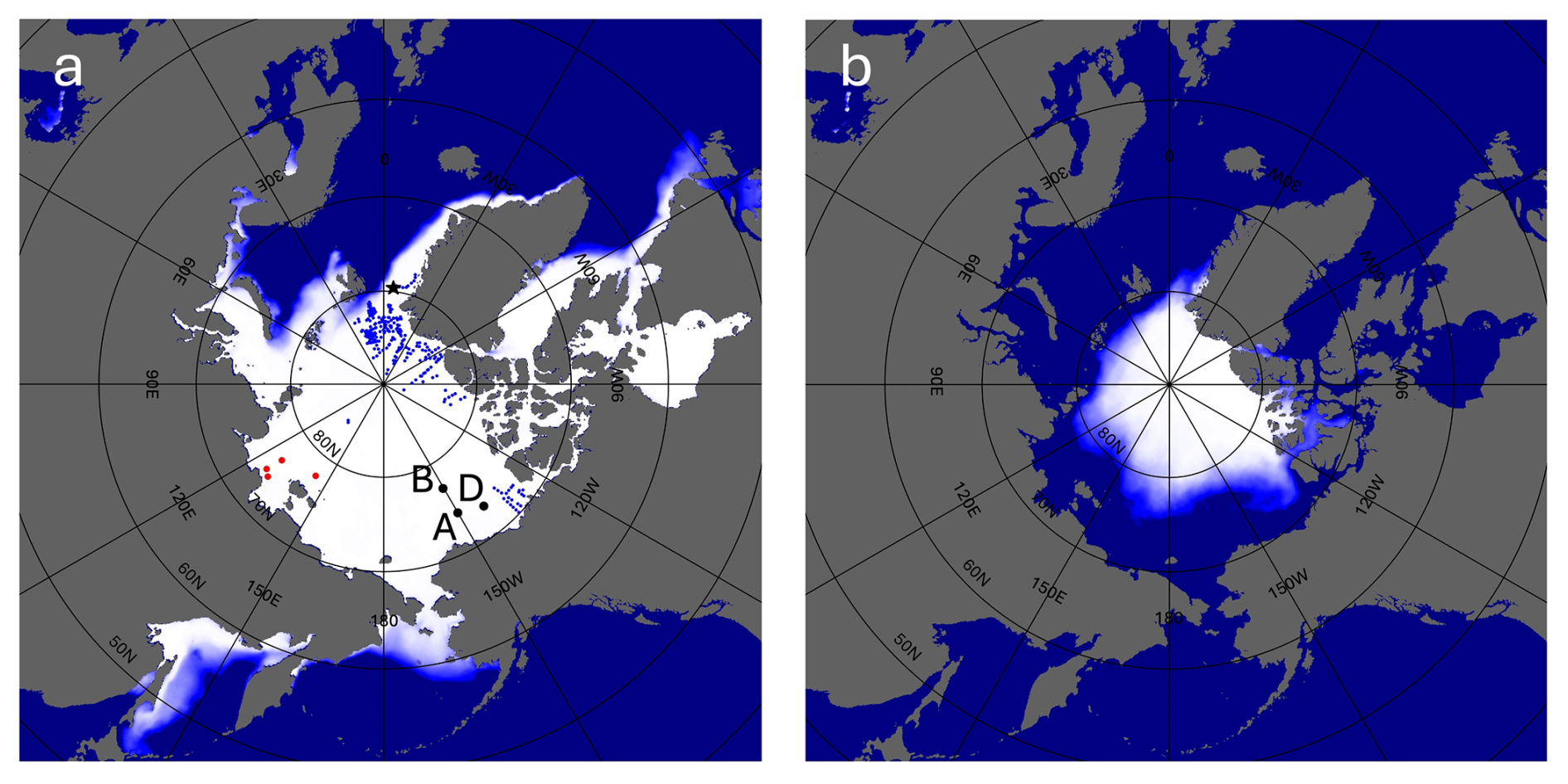
Figure 1 Sea ice concentration in the Northern Hemisphere averaged over the period from 2013 to 2024. (a) March average, representing the typical winter maximum. Observational sites used in this study are indicated: black dots labeled A, B, and D represent ULS moorings in the Beaufort Sea; black stars indicate ULS moorings in the Fram Strait; red dots indicate Upwardlooking ADCP moorings in the Laptev Sea (four sites); and blue dots indicate airborne EM observation points. All these sites are used in Sect. 4. (b) September average, representing the typical summer minimum. White areas indicate sea ice extent.

To overcome the limitations of individual sensors, hybrid and data-fusion approaches have been developed. A key example is the SMOS–CryoSat product, which merges passive microwave and radar altimetry data to improve thickness estimates across both thin and thick ice regimes  (Ricker et al., 2017). Similarly, the ESA CCI Envisat product provides a long-term, altimetry-based thickness record for the pre-CryoSat era (Hendricks et al., 2018), while more recent neural-network approaches aim to homogenize multi-mission altimetry measurements from ERS, Envisat, and CryoSat-2 into consistent thickness fields (Bocquet et al., 2023). Passive microwave-based machine-learning retrievals have also emerged, extending thin-ice estimation to multi-decadal time periods using SSM/I and SSMIS brightness temperatures (Soriot et al., 2024). In parallel, several studies have refined CryoSat-2 thickness estimates by improving snow loading assumptions and freeboard processing (Nab et al., 2024). In addition to observation-only approaches, numerical data assimilation systems such as PIOMAS combine satellite data, in situ records, and ocean-ice models to generate temporally continuous thickness fields (Schweiger et al., 2011; Schweiger et al., 2019). More recently, hybrid machine-learning and data-assimilation strategies have been proposed to reconstruct historical thickness fields prior to the satellite altimetry era, offering improved consistency over multiple decades (Edel et al., 2025).

In situ observations remain crucial for validating satellite-derived thickness estimates. Field campaigns utilize various measurement techniques, including electromagnetic (EM) induction sounding, ULS moorings, and ice core drilling. EM sensors, deployed from aircraft or directly on the ice, provide spatially extensive but surface-biased measurements (Haas et al., 2008; Haas et al., 2009). ULS moorings, positioned beneath the ice, offer continuous time series of ice draft, which can be converted to thickness assuming a known ice density (Melling et al., 1995). Ice core drilling provides direct thickness measurements along with information on ice structure and salinity (e.g. Worby et al., 2008) but is limited in spatial coverage. These observations are essential for evaluating the performance of satellite retrieval algorithms and improving model parameterizations.

Despite advances in satellite-based retrievals of sea ice thickness, achieving spatially and temporally consistent estimates across diverse ice regimes and seasons remains challenging. Many existing methods rely on region-specific empirical relationships, which are subject to uncertainties in key parameters such as snow cover and ice salinity. Reanalysis datasets like PIOMAS provide comprehensive estimates, but their reliance on numerical models introduces systematic biases and uncertainties stemming from imperfect model physics and data assimilation techniques.

In this study, we propose a novel approach to deriving sea ice thickness using a trajectory-based framework (e.g. Korosov et al., 2018), based on sea ice motion data derived from passive microwave radiometer observations. By tracking sea ice backward in time, we identify its formation date and location to reconstruct its age distribution based on daily changes in ice concentration. Along each trajectory, the cumulative surface heat budget is used as a measure of ice growth potential, and estimated ice thickness is obtained by scaling this measure to ULS observations.

This history-based approach provides a new perspective on sea ice monitoring by explicitly incorporating the temporal evolution of individual sea ice. Unlike traditional methods that assume static empirical relationships between radiative properties and thickness, our method reflects the cumulative growth processes experienced by the ice. This enables the creation of spatially and temporally continuous sea ice thickness datasets based entirely on observational data, mitigating some of the uncertainties inherent in empirical and model-based approaches.

Through the development and validation of this method, which combines a growth-tracking model with passive microwave observations, we aim to enhance monitoring capability of sea ice thickness from passive microwave observations and contribute to a deeper understanding of polar climate dynamics.

2 Data

This study used two types of satellite-derived sea ice data: sea ice concentration and sea ice drift velocity. Daily sea ice information was derived from passive microwave satellite observations. Data from January 2003 to August 2011 were obtained from the Advanced Microwave Scanning Radiometer for EOS (AMSR-E). AMSR-E observations ceased in October 2011, while Advanced Microwave Scanning Radiometer 2 (AMSR2) began operation in July 2012. Accordingly, this study used AMSR-E data from January 2003 to September 2011, and AMSR2 data from July 2012 to the most recent available observations (as of December 2024).

Sea ice drift velocity data were derived from gridded brightness temperature in both horizontal and vertical polarization channels. The datasets were provided by the Japan Aerospace Exploration Agency (JAXA) and projected onto a 10×10 km polar stereographic grid. They are publicly available via the Arctic and Antarctic Data Archive System (ADS) of the National Institute of Polar Research, Japan. Ice motion was derived using 36 GHz brightness temperatures in winter (December–April) due to their finer spatial resolution, and 18 GHz data in summer (May–November) because of their reduced sensitivity to surface melt and varying surface conditions.

Ice drift was calculated using a pattern-matching technique known as the maximum cross-correlation method (Ninnis et al., 1986; Emery et al., 1991). This method identifies the spatial offset that maximizes the cross-correlation coefficient between two consecutive daily images. After filtering and interpolation, a daily sea ice velocity dataset was constructed on a 60×60 km grid, with no missing values across the ice-covered region. The accuracy of this ice motion dataset was evaluated by Sumata et al. (2018), who demonstrated consistent performance throughout the year. This dataset has also been used in long-term sea ice trajectory analyses (Kimura et al., 2013; Kimura et al., 2020), showing minimal positional error even after tracking ice motion over an entire year. Kimura et al. (2013) demonstrated that, even after five months of particle tracking, the positional error relative to drifting buoys remained below 50 km, even in regions with the largest discrepancies.

Daily ice concentration data were computed using a bootstrap algorithm (Comiso, 2009) based on the 18 and 36 GHz brightness temperatures from AMSR-E and AMSR2. These data, provided on a 10 km grid, were produced by JAXA and distributed via the ADS.

In addition, this study utilized in situ observations of sea ice thickness from moored upward-looking sonar (ULS) instruments. For the Beaufort Sea, sea ice draft data were obtained from the Beaufort Gyre Exploration Project (BGEP), maintained by the Woods Hole Oceanographic Institution (WHOI). Ice draft, defined as the vertical distance from the waterline to the bottom of the sea ice, was multiplied by 1.1 (e.g. Fukamachi et al., 2017) to estimate total sea ice thickness. ULS observations were conducted at 1 s intervals, yielding up to 86 400 measurements per day. Although BGEP includes four mooring sites, this study used data from three locations: Mooring A (75° N, 150° W), Mooring B (78° N, 150° W), and Mooring D (74° N, 140° W), which provide long-term, continuous records of sea ice draft. These data were used both to develop the sea ice thickness estimation method and to evaluate its accuracy.

To assess the applicability of the method to other regions, we used additional mooring observation data from the Fram Strait and the Laptev Sea. For the Fram Strait, ULS data from the Arctic Outflow Observatory operated by the Norwegian Polar Institute (Sumata et al., 2022) were used. Specifically, sea ice draft data at Mooring F11 (78.8° N, 3.0° W) from 2016 to 2018 were available as daily mean values. For the Laptev Sea, upward-looking Acoustic Doppler Current Profilers (ADCPs) data were obtained from Belter et al. (2020), covering the period from September 2007 to August 2011 at four mooring sites (74.33° N, 128.01° E; 74.72° N, 125.28° E; 76.57° N, 126.06° E; and 77.99° N, 143.01° E). These Laptev Sea observations were also provided as daily mean sea ice draft. For both regions, effective sea ice thickness was estimated by multiplying the ice draft by 1.1 and by the sea ice concentration, in order to maintain consistency with the approach used for the Beaufort Sea.

To complement these point-based measurements, we also used airborne electromagnetic (EM) ice thickness observations conducted by the Alfred Wegener Institute (Haas et al., 2009). These surveys cover wide areas of the western Arctic Ocean and provide spatially extensive and independent measurements for validating the satellite-derived sea ice thickness estimates.

For the surface heat budget calculations in Sect. 4, we used the following ERA5 variables (Muñoz Sabater, 2019): mean sea level pressure, 10 m wind, 2 m air temperature, 2 m dewpoint temperature, surface solar radiation downward, surface thermal radiation downward, and sea surface temperature.

3 Estimation of sea ice age

To investigate the origin and drift history of sea ice, we performed a backward trajectory analysis using Lagrangian particles. Particles were initialized at 10 km intervals within areas where sea ice concentration exceeded 15 %, with their daily positions adjusted to reflect changes in the spatial distribution of sea ice. Gridded sea ice velocity data were used to calculate daily displacements with a one-day time step, and particle velocities were interpolated from surrounding grid points using a Gaussian distance-weighted average.

Each particle was tracked backward in time for up to four years. When a particle entered an area where sea ice concentration fell below 15 %, that location was designated as its formation site. If a particle did not reach such a region within four years, its position at the end of the four-year tracking was treated as the formation site. A four-year tracking period was adopted to maximize the temporal coverage of the derived products. Extending the tracking period would delay the earliest date at which ice age and thickness can be estimated from the beginning of the AMSR-E record, and it would further reduce the available record after the AMSR-E–AMSR2 data gap. Because sea ice older than four years occupies only a small fraction of the Arctic, this choice has little impact on the resulting ice age and thickness estimates.

Figure 2 illustrates examples of these backward trajectories initialized on 31 May 2021, showing particle locations one, two, and three years prior. Dark blue dots represent particles still in transit, while light blue dots indicate their inferred formation sites. 89 % of the particles reached their formation sites within three years, suggesting that ice older than three years is relatively rare. The spatial distribution of formation sites (light blue dots) suggests that most sea ice originates in regions stretching from the Beaufort Sea to the Russian marginal seas, areas typically ice-free during summer (consistent with the difference between Fig. 1a and b). Notably, ice formation was not confined to coastal polynyas; rather, extensive offshore ice production was observed, indicating a key characteristic of regional ice generation. In Krumpen et al. (2019), the backward trajectories of sea ice in the Fram Strait were tracked, and the resulting ice distribution closely resembles that observed here.

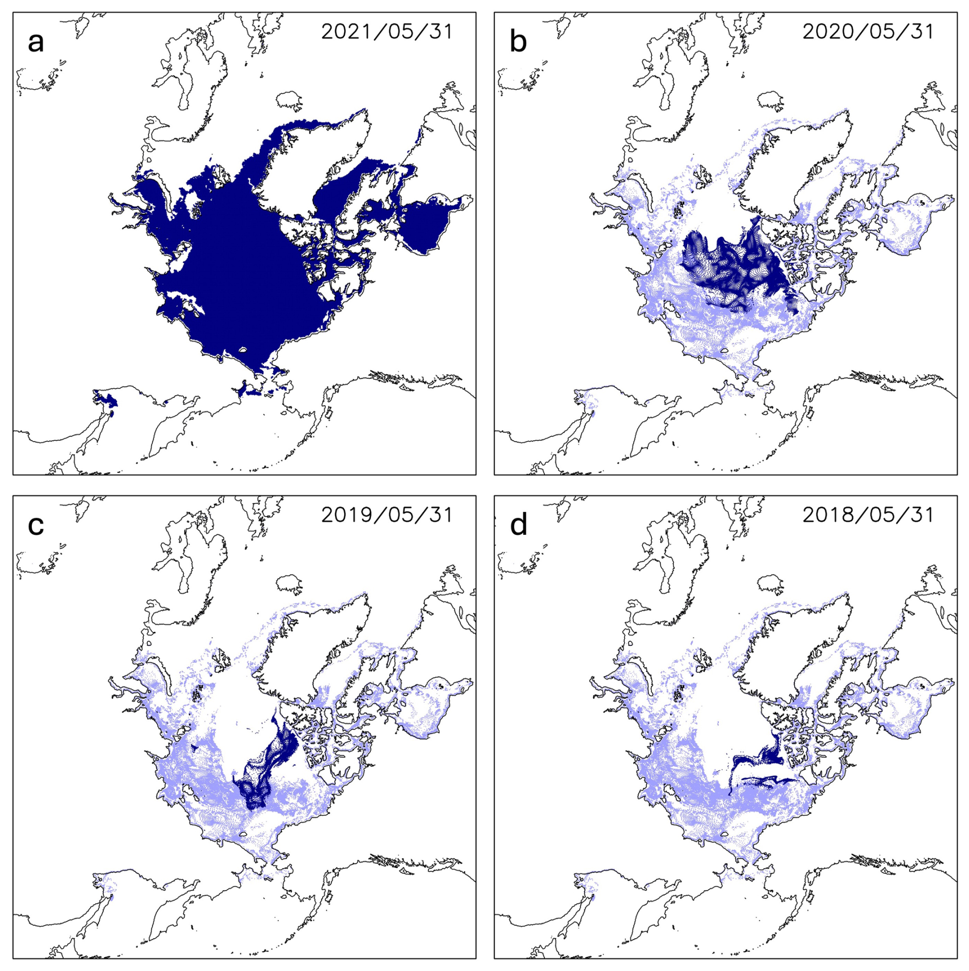
Figure 2 Backward-tracked positions of particles initially distributed over the sea ice on 31 May 2021. Particles were placed at 10 km intervals over the ice and tracked backward in time. Dark blue dots show particle positions on (a) 31 May 2021, (b) 31 May 2020, (c) 31 May 2019, and (d) 31 May 2018. Light blue dots mark the positions where particles reached open water.

It is important to note that these particles do not represent individual ice floes. The estimated formation date and location reflect the oldest ice within the area represented by each particle, approximately a 10×10 km region. Although the particles themselves follow fixed trajectories, the sea ice within their represented areas is continually replaced by daily processes of melting, formation, and advection. Therefore, instead of assigning a single age value to each particle, we computed a full age distribution, that is, a frequency distribution of sea ice age categories, at each particle's location. This age distribution evolves over time as sea ice forms, melts, and advects.

To capture temporal changes in the sea ice age distribution at each particle's location, we estimated daily net ice formation using the method proposed by Kimura and Wakatsuchi (2004, 2011). This method attributes changes in sea ice area at each pixel to local thermodynamic and dynamic processes (e.g., freezing, melting, and deformation) as well as ice transport. The daily change in ice-covered area is expressed as

$$\begin{array}{}\text{(1)}& A(t+\mathrm{1})-A\left(t\right)=P\left(t\right)+F_{\mathrm{in}}\left(t\right)\end{array}$$

where A(t) is the ice-covered area on day t, computed as ice concentration multiplied by the pixel area (10 × 10 km²). P(t) denotes local net ice production or melt, and F_in(t) is the ice area advected into the pixel from neighboring cells. F_in(t) represents changes due to convergence or divergence of sea ice, and does not account for apparent area reduction caused by dynamic deformation (e.g. ridging or rafting).

Equation (1) represents the area budget of sea ice. In reality, sea ice area decreases due to both thermodynamic melting and dynamical deformation. In the present formulation, these contributions are not explicitly separated. Instead, P(t) is interpreted as the net apparent area change, including both thermodynamic and dynamical contributions to area loss. This simplification was adopted because deformation-induced area loss cannot be robustly quantified from available observations at basin scale. Although this approach does not explicitly represent overlapping ice floes of different ages, its impact on the estimated age composition is expected to be limited, and it provides a practical and internally consistent approximation suitable for basin-scale reconstruction of sea ice age distribution.

When P(t) was positive, it was interpreted as the area of newly formed ice for that day. In this case, the fractional increase in total ice area was assigned to newly formed ice, and the age distribution was updated by adding this amount to the youngest age class. Conversely, when P(t) was negative – indicating a net loss of ice area – the ice in all age classes was reduced proportionally according to the loss ratio. For example, if P(t) indicated a 5 % decrease, the amount of ice in every age category was reduced by 5 %. Although younger, thinner ice is more likely to melt first in reality, this preferential melting effect was neglected for simplicity. By cumulatively applying these daily gains and losses, we obtained the evolving frequency distribution of sea ice age at each location. This procedure allowed us to reconstruct the full daily evolution of age distribution along each particle trajectory.

Figure 3b presents the evolution of sea ice age distribution along the trajectory of a representative particle (shown in Fig. 3a). At the locations along the particle's trajectory, sea ice began forming on 1 October 2017 and reached 100 % concentration by 18 October. In the following summer, the concentration temporarily decreased to 40 %–50 % but generally remained high. Ice formed during the first year (prior to 10 September 2018) declined rapidly in September 2018, and by 31 May 2021 accounted for only 0.2 % of the ice cover at that location. Ice formed between 10 September 2018 and 10 September 2019 accounted for approximately 10  % of the total area, as can be seen in more detail in the age distribution shown in Fig. 4.

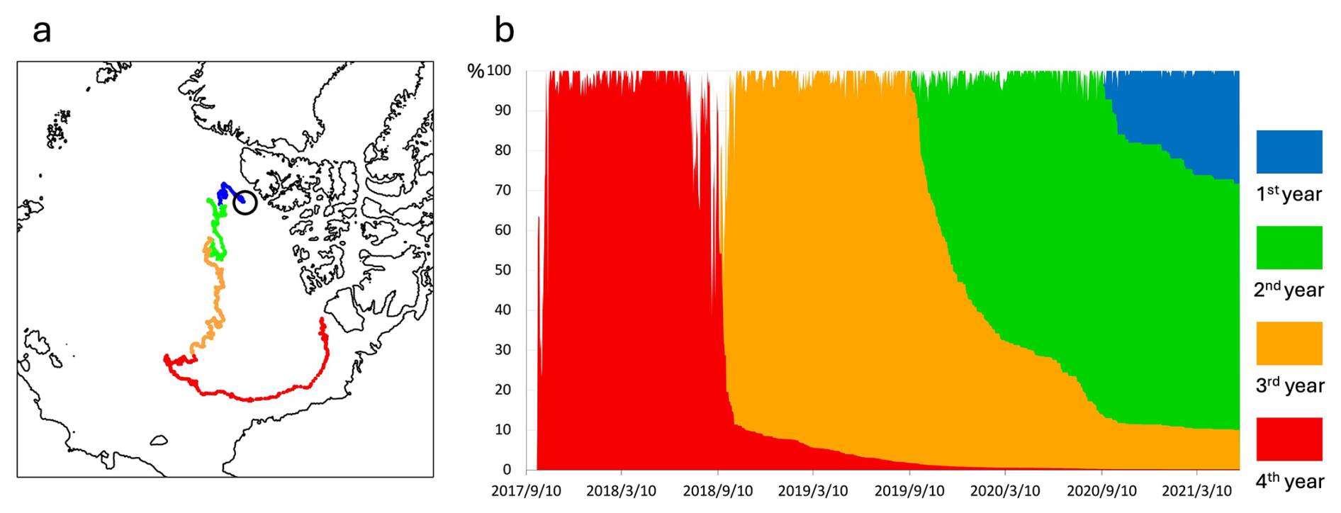
Figure 3 (a) Backward trajectories of a synthetic sea ice particle initialized on 31 May 2021 (white circle). The colored lines represent the particle's drift path in different time periods: blue for 10 September 2020–31 May 2021, green for 10 September 2019–10 September 2020, orange for 10 September 2018–10 September 2019, and red for before 10 September 2018. The earliest traced date corresponds to 1 October 2017, which is considered the formation date of the sea ice. (b) Time series of the ice concentration along the particle's trajectory from 10 September 2017 to 31 May 2021. The vertical axis represents ice concentration (%). The stacked colored areas show the fractional contributions of ice formed in each period: red for ice formed before 10 September 2018, orange for 10 September 2018–10 September 2019, green for 10 September 2019–10 September 2020, and blue for after 10 September 2020. Initially, the ice concentration quickly increases to nearly 100 % and remains high throughout the lifetime.

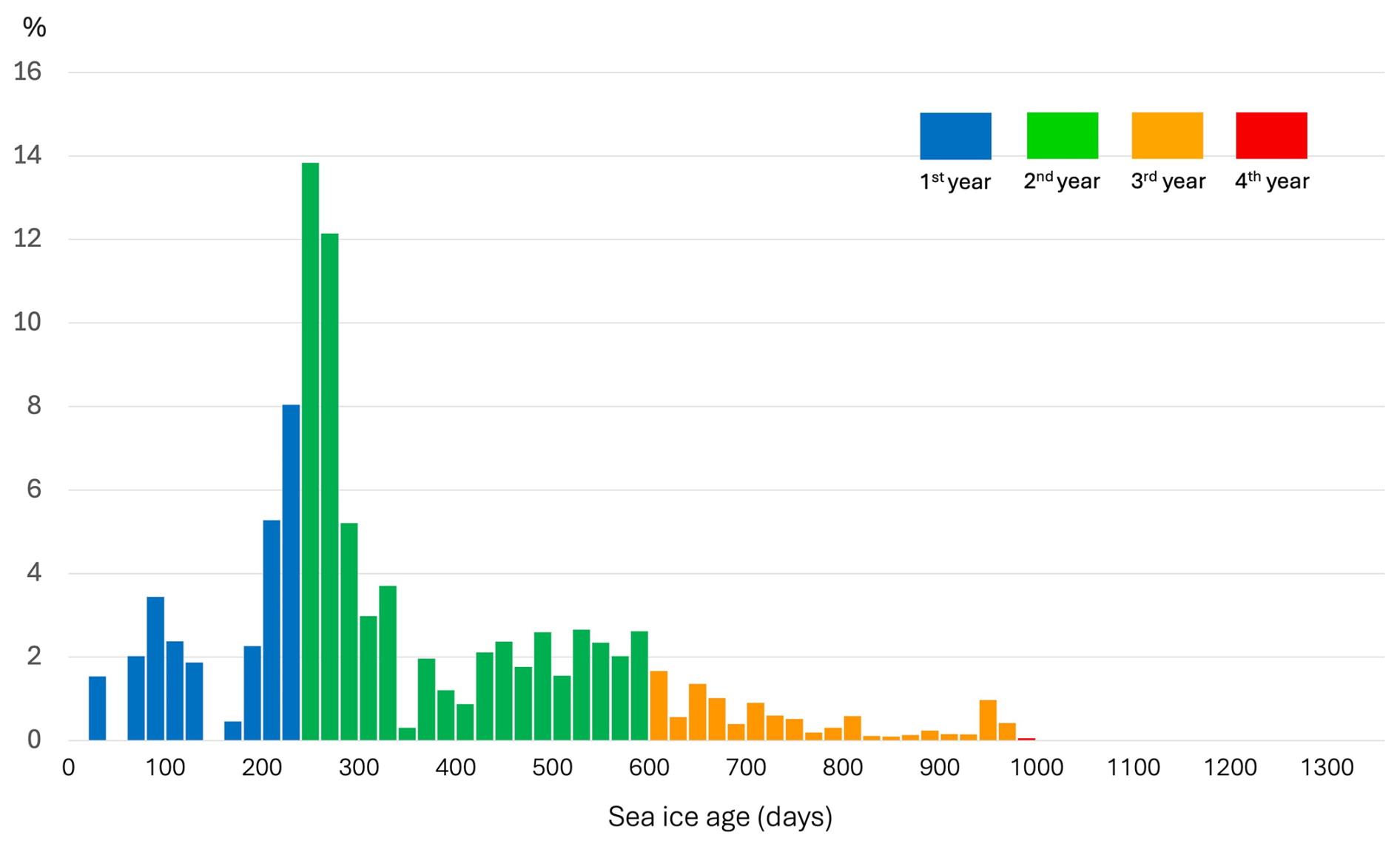
Figure 4 Sea ice age distribution on 31 May 2021. The horizontal axis shows sea ice age in 20 d intervals, and the vertical axis represents the percentage of total sea ice area. Colors indicate the formation period: red for ice formed before 10 September 2018, orange for 10 September 2018–10 September 2019, green for 10 September 2019–10 September 2020, and blue for after 10 September 2020.

Figure 4 shows the sea ice age distribution on 31 May 2021 at the location of the representative particle marked by the white circle in Fig. 3a, which represents the starting point of its backward trajectory. Although a very small fraction of ice older than three years persisted, the majority was relatively young, having formed during the most recent summer–autumn season. This age distribution forms a key basis for estimating sea ice thickness. The age distribution can be computed for any day and location throughout the ice-covered region. Based on this information, we can determine the age of the oldest ice present at each location. For example, in Fig. 4, the oldest ice was formed on 1 October 2017, making it 1339 d old as of 31 May 2021. Knowing the oldest ice age at a given location is useful for estimating the maximum possible ice thickness in that area. It also provides insight into the survival and persistence of multiyear ice, which is critical for understanding long-term changes in ice stability, structural strength, and resistance to melt.

Figure 5a displays the spatial distribution of the oldest ice age on 31 May 2021. Furthermore, by weighting the age by their respective area fractions (as shown in Fig. 4), we estimated the mean sea ice age at each location. Figure 5b shows the corresponding spatial distribution of mean sea ice age. Both maps indicate that older sea ice is concentrated in the western part of the Arctic Ocean, particularly north of the Canadian Arctic Archipelago and Greenland. This region is well known as a reservoir for multiyear ice due to its relatively stable and low-export conditions, which allow sea ice to survive through multiple melt seasons. In contrast, the Siberian side and marginal seas are dominated by younger ice, consistent with high melt rates and dynamic ice export. Whereas the oldest ice age represents the maximum age of ice present in each grid cell, the mean age reflects the overall age distribution. It tends to be lower, particularly in transitional regions where old ice is mixed with recently formed ice. This difference highlights the importance of considering both indices to fully characterize the spatial structure and renewal dynamics of Arctic sea ice.

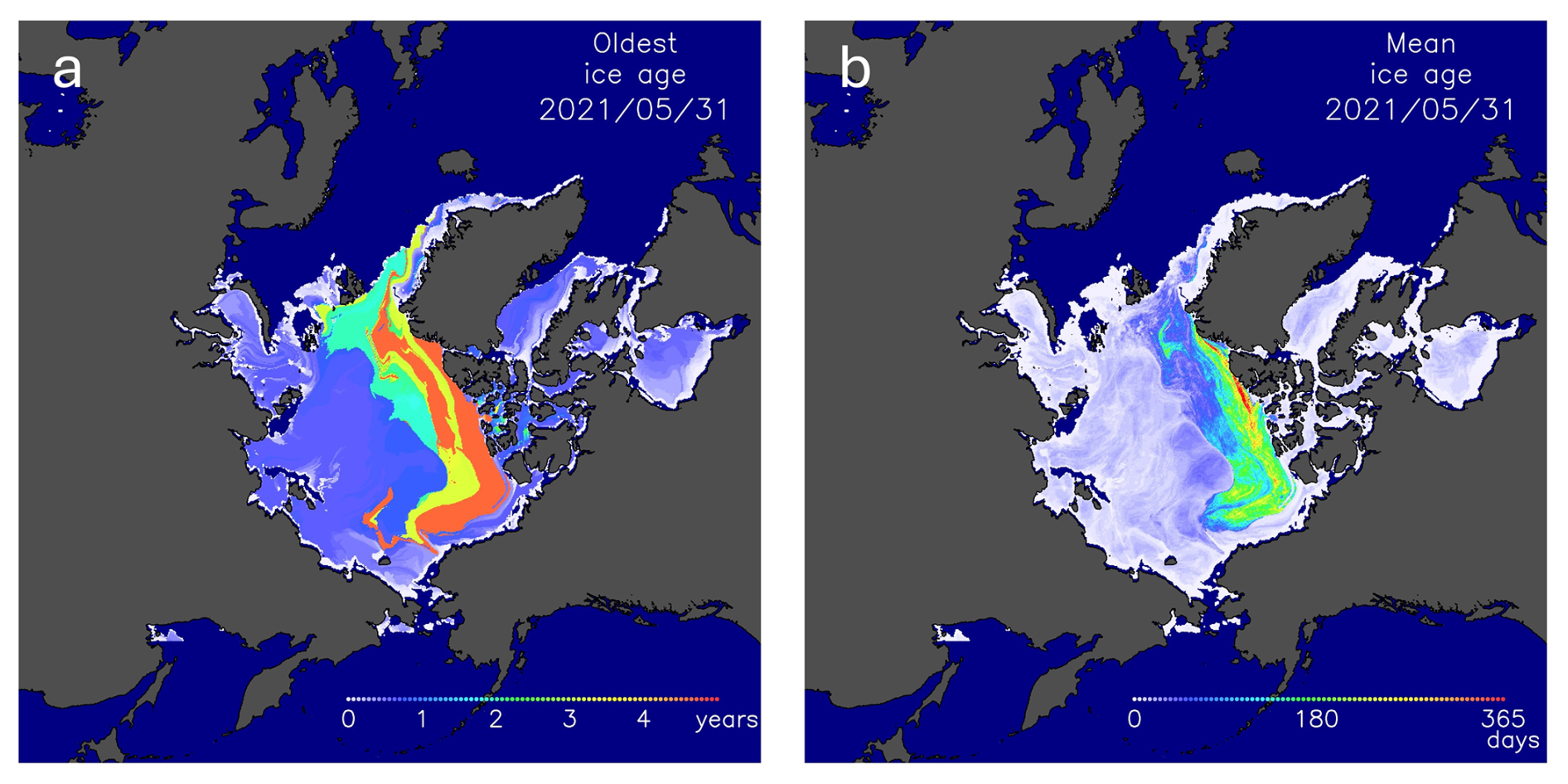
Figure 5 Spatial distribution of sea ice age on 31 May 2021. (a) Oldest sea ice age at each grid cell, showing the maximum age of ice present. (b) Mean sea ice age at each grid cell, calculated as the area-fraction-weighted average age of all ice within the cell. Color bars show ice age in years (a) and days (b).

Figure 6 presents the monthly averaged mean sea ice age in 2021. A notable feature is the seasonal retreat of older sea ice extending into the Beaufort Sea. This region, which contains relatively old ice (indicated in yellow to red), gradually diminishes during the melt season from July through September, indicating significant loss of multiyear ice in this area. By September, the Beaufort Sea is largely covered by first-year ice or is ice-free. Although the oldest ice remains largely confined to the central Arctic Ocean, its spatial extent and location show some variability, indicating ongoing advection and redistribution of long-lived ice floes.

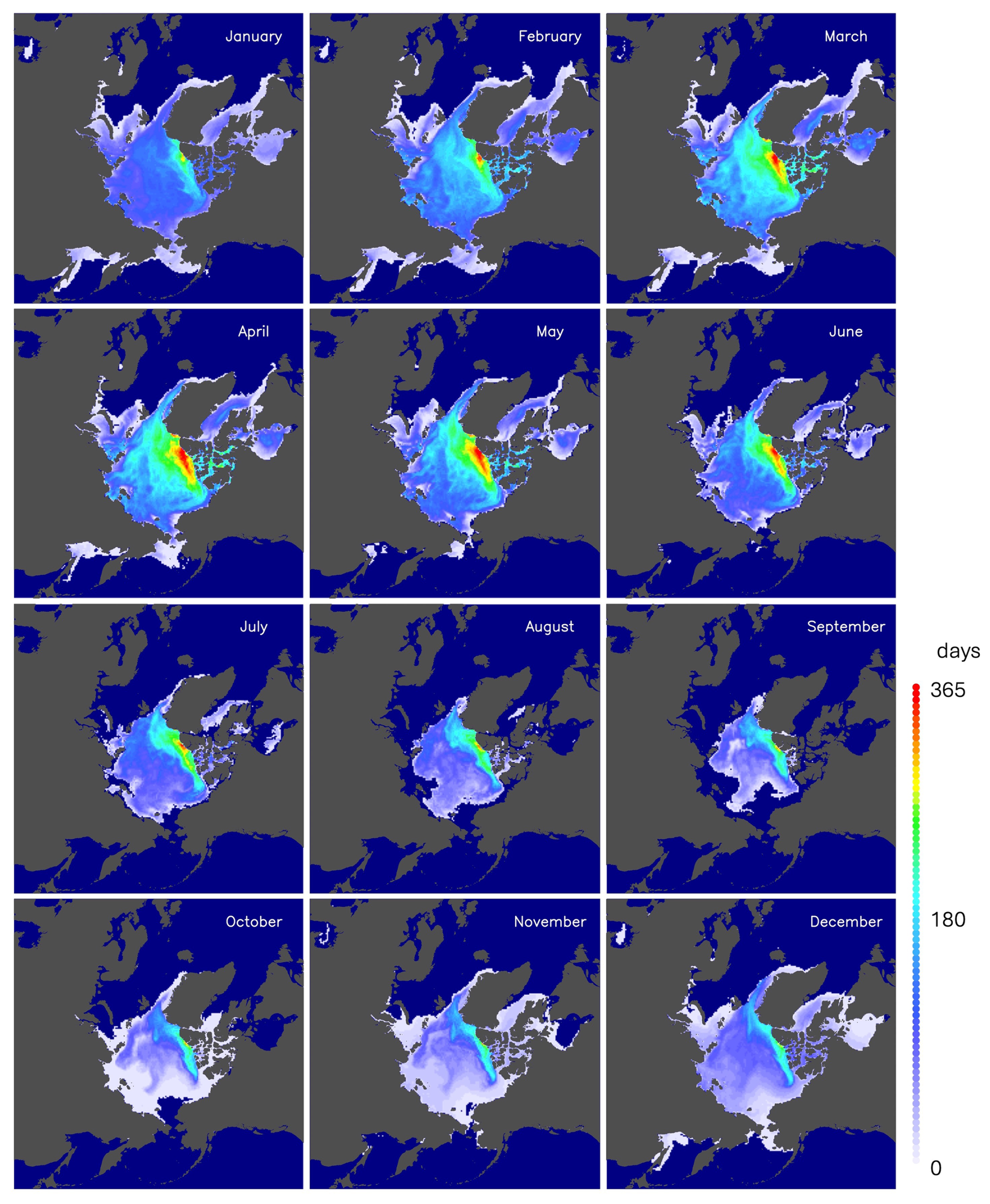
Figure 6 Monthly averages of the mean sea ice age for each month in 2021.

4 Estimation of sea ice thickness

The mean sea ice age map shown in Fig. 5b resembles the well-known patterns of sea ice thickness distribution (e.g. Bourke and Garrett, 1987). However, the actual ice thickness is not determined by age alone, as the ice continues to experience growth and melt under varying environmental conditions after its formation. To better characterize the conditions under which the ice was exposed to growth-favorable environments, we calculated the potential ice growth using a surface heat budget approach following Toyota et al. (2022). The surface heat flux was derived from ERA5 reanalysis data, incorporating sensible and latent heat fluxes, shortwave radiation, and net longwave radiation. Sensible and latent heat were estimated using the bulk method, with typical transfer coefficients and atmospheric parameters. The absorbed shortwave flux was calculated assuming a constant albedo (0.07, a typical value for open water), and net longwave flux combined ERA5 downward radiation with outgoing flux computed using the Stefan–Boltzmann law. Finally, potential daily ice growth was computed from the total surface heat flux and the latent heat of fusion, assuming standard values for ice density and salinity.

For the calculation, we assumed open-water conditions throughout the ice lifetime. This calculation does not provide a direct measure of ice thickness; rather, it is performed to obtain a quantitative parameter representing the cumulative potential growth. The open-water assumption also allows the implicit inclusion of dynamically thickened ice, as discussed further in Sect. 5.

Cumulative growth was obtained by integrating daily growth from the time of ice formation to the present, with negative values set to zero. This procedure was applied to all sea ice age classes present at each particle location. For example, ice formed one day earlier received one day of cumulative growth, whereas ice formed 1000 d earlier received 1000 d of cumulative growth. The cumulative growth for each age class was weighted by its fractional area to obtain the mean cumulative growth at each particle location. The resulting cumulative growth was finally scaled using a factor derived from comparison with in situ observations to match observed ice thickness.

Figure 7 compares the estimated mean cumulative growth with the observed daily mean sea ice thickness from ULS measurements in the Beaufort Sea. The temporal variations of the two datasets show excellent agreement, indicating that the cumulative growth serves as a reliable indicator of actual ice thickness trends. To make the cumulative growth comparable to the observed thickness, we multiplied it by a constant scaling factor of 0.25, empirically chosen to provide the best fit to the observed daily mean thickness across all three mooring sites (A, B, and D). It should be noted that this value of 0.25 was derived from data fitting and does not have a direct physical interpretation. The scaled cumulative growth (red line in Fig. 7) represents the estimated ice thickness. The applicability of this factor to other regions is evaluated below.

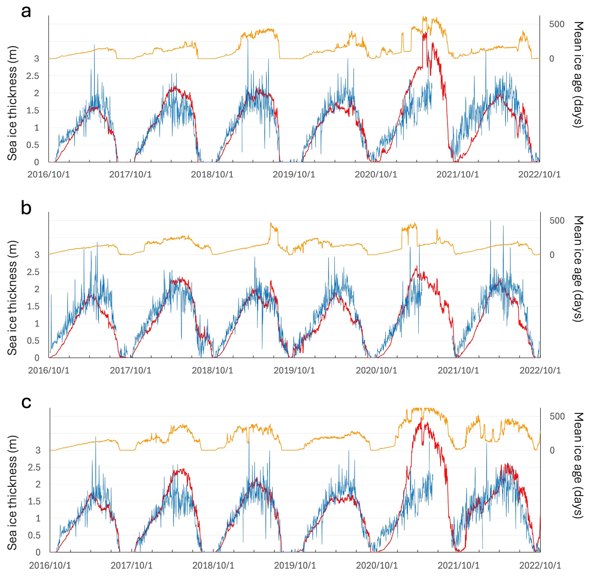
Figure 7 Time series of sea ice thickness and mean ice age at three mooring sites. Panels show data from (a) site A, (b) site B, and (c) site D, corresponding to the locations marked in Fig. 1a. Blue lines indicate sea ice thickness observed by ULS, red lines show estimated sea ice thickness, and orange lines represent the mean sea ice age. The time period is from 1 October 2016 to 1 October 2022. Left vertical axes indicate sea ice thickness, and right vertical axes indicate mean sea ice age.

At all three mooring sites, the seasonal evolution of ice thickness shows a similar pattern, with growth beginning in autumn, peaking in late winter, and declining during the melt season. The orange line represents the evolution of mean sea ice age, which varies substantially from year to year in this region, reflecting the variable inflow of older, thicker ice from the Canadian Arctic Archipelago. The agreement between the estimated and observed values is remarkably good, indicating that surface heat budget history is a strong predictor of sea ice thickness. For example, at Mooring A (Fig. 7a), older ice was more prevalent in 2018–2019 and 2020–2021, yet the observed sea ice thickness remained comparable to other years. This aligns with the findings of Mahoney et al. (2019), who showed that even multiyear ice that survives summer melt becomes indistinguishable in thickness from first-year ice by the end of winter, based on similar ULS data combined with buoy and satellite tracking.

Although the estimated ice thickness successfully captures overall trends, some discrepancies are evident. For instance, at Moorings A (Fig. 7a) and D (Fig. 7c), our calculation overestimated ice thickness during 2020–2021, when older ice dominated. This suggests that the method may overestimate thickness in regions where the mean sea ice age exceeds 500 d, particularly for thicker, long-lived ice. In addition, this overestimation may be attributed to errors in the backward trajectory analysis, which could lead to an overestimation of sea ice age itself. However, because actual sea ice age cannot be directly observed, it is difficult to determine which factor is primarily responsible for the discrepancy.

To further assess the broader applicability of our method, we compared estimates with ULS observations from different regions. Figure 8 presents the effective ice thickness derived from ULS observations (also shown in Fig. 2 of Sumata et al., 2022), alongside our estimated ice thickness at the corresponding location in the Fram Strait (marked by a star in Fig. 1a). The Fram Strait is the primary gateway for sea ice export from the Arctic Ocean into the North Atlantic, and thus the sea ice passing through this region reflects a wide range of thickness and age conditions originating from across the Arctic Basin. The estimates were calculated using the method described above, without incorporating the Fram Strait ULS data. The two datasets show excellent agreement in both seasonal and interannual variability, capturing features such as the thicker ice in 2016–2017 and thinner ice in 2017–2018. Moreover, our method successfully captures rapid changes in ice thickness on shorter timescales, such as sharp growth and decay events during the freezing and melting seasons.

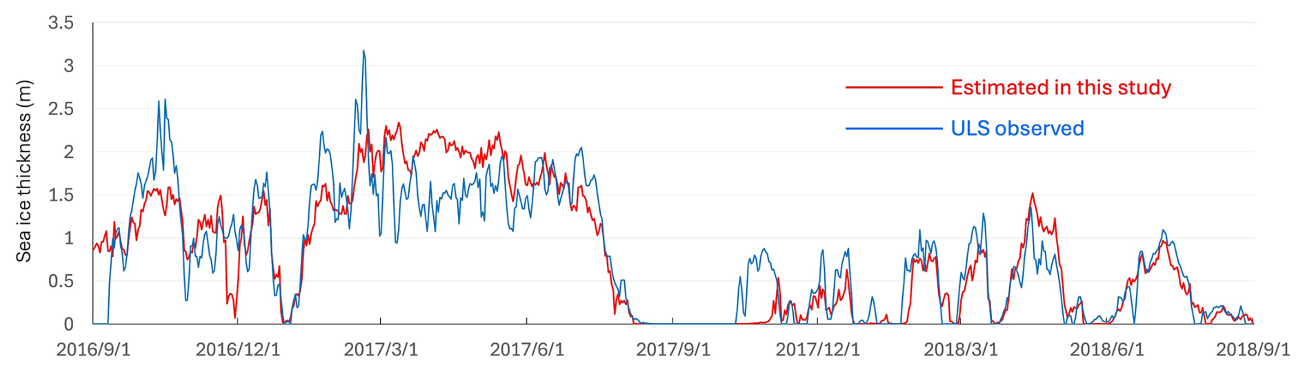
Figure 8 Comparison of sea ice thickness estimated in this study (red line) with observed ice thickness (blue line) by ULS at the Fram Strait mooring site (labeled F in Fig. 1a) from 1 September 2016 to 1 September 2018. The observed values represent the effective ice thickness presented in Sumata et al. (2022).

Figure 9 presents time series of daily mean sea ice thickness observed by moored upward-looking ADCPs in the Laptev Sea together with the corresponding thickness estimated from our method. The locations of the moorings are shown in the map in the lower-right panel. This region is characterized by the absence of multiyear ice and is dominated by first-year ice throughout the winter. Overall, the seasonal evolution of ice thickness is captured well at all four sites: the timing of initial freeze-up, the gradual thermodynamic growth through winter, and the onset of melt are broadly consistent between the observations and the estimates. However, two systematic differences are evident. First, during the early stages of ice formation in autumn, the observed thickness increases more rapidly than the estimate. Second, the observed thickness exhibits pronounced day-to-day variability, particularly at the moorings closer to the coast (Fig. 9c, d), which show intermittent episodes of very thick ice. These large fluctuations indicate strong horizontal heterogeneity in ice thickness, likely associated with dynamic deformation events. In these periods, the estimated thickness tends to follow the lower envelope of the observations, systematically underestimating the larger peaks. This contrast between the smoother evolution of the estimates and the highly variable observations highlights the influence of active deformation in this region, which is not represented in our thermodynamic framework.

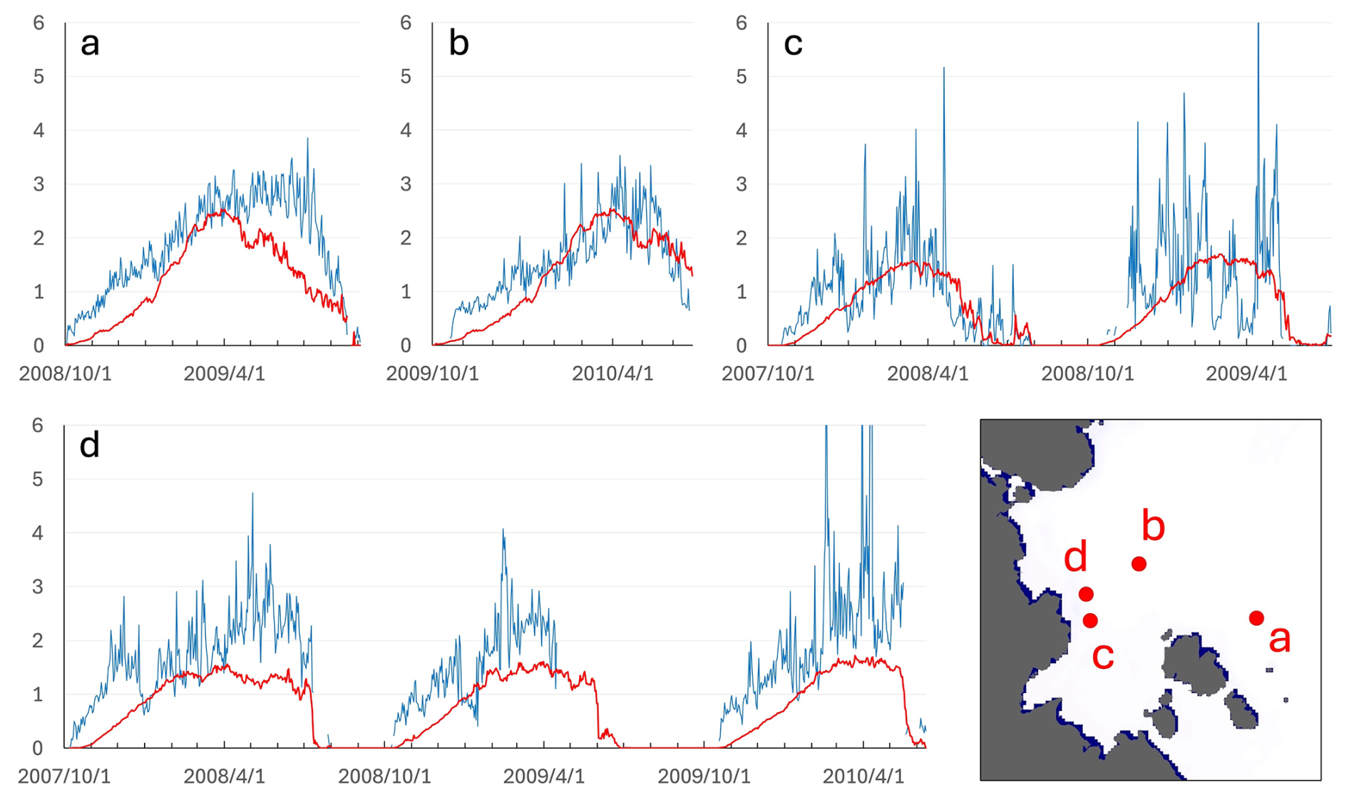
Figure 9 Time series of daily sea ice thickness observed by four ADCP moorings in the Laptev Sea (blue lines) and the corresponding thickness estimated using our method (red lines). Panels (a)–(d) show data from the four mooring sites. The map in the lower-right panel provides a close-up view of the Laptev Sea and indicates the locations of the ADCP moorings.

To evaluate the overall consistency and regional applicability of our method, Fig. 10 compares observed and estimated sea ice thickness across four Arctic regions. Each panel shows a scatter plot of observed versus estimated thickness, along with reference lines corresponding to scaling factors of 0.15, 0.25, and 0.35. In the Beaufort Sea (Fig. 10a; n=6042), which uses the same ULS dataset as in Fig. 7, the data exhibit a strong linear relationship (correlation = 0.83) with an RMS error of 44.0 cm. The points align closely with the 0.25-scaling line, indicating that this factor appropriately represents the local relationship between the observed and estimated values. In the Fram Strait (Fig. 10b; n = 731), the correlation is similarly high (0.87) with an RMS error of 36.3 cm, again consistent with the 0.25 scaling. In the Laptev Sea (Fig. 10c; n = 1952), based on ADCP-derived ice-draft data, the correlation is slightly lower (0.73) and the RMS error increases to 86.4 cm. As discussed earlier, many observed values exceed the estimates because the observations include episodic occurrences of very thick ice, reflecting strong deformation activity in this region. Although applying a larger scaling factor (e.g., 0.35) would reduce the RMS error, we argue that such discrepancies should instead be addressed in future versions of the dataset by explicitly incorporating the effects of dynamic thickening. Finally, the comparison at the EM observation sites shown as blue points in Fig. 1a (Fig. 10d; n = 279) yields a correlation of 0.62 and an RMS error of 90.6 cm. When the observed values are shifted upward by 1 m, the relationship aligns well with the 0.25 scaling line, consistent with the results from the Beaufort Sea and Fram Strait. Overall, these comparisons demonstrate that our approach performs consistently across a wide range of Arctic environments, supporting its robustness in both spatial and temporal applications.

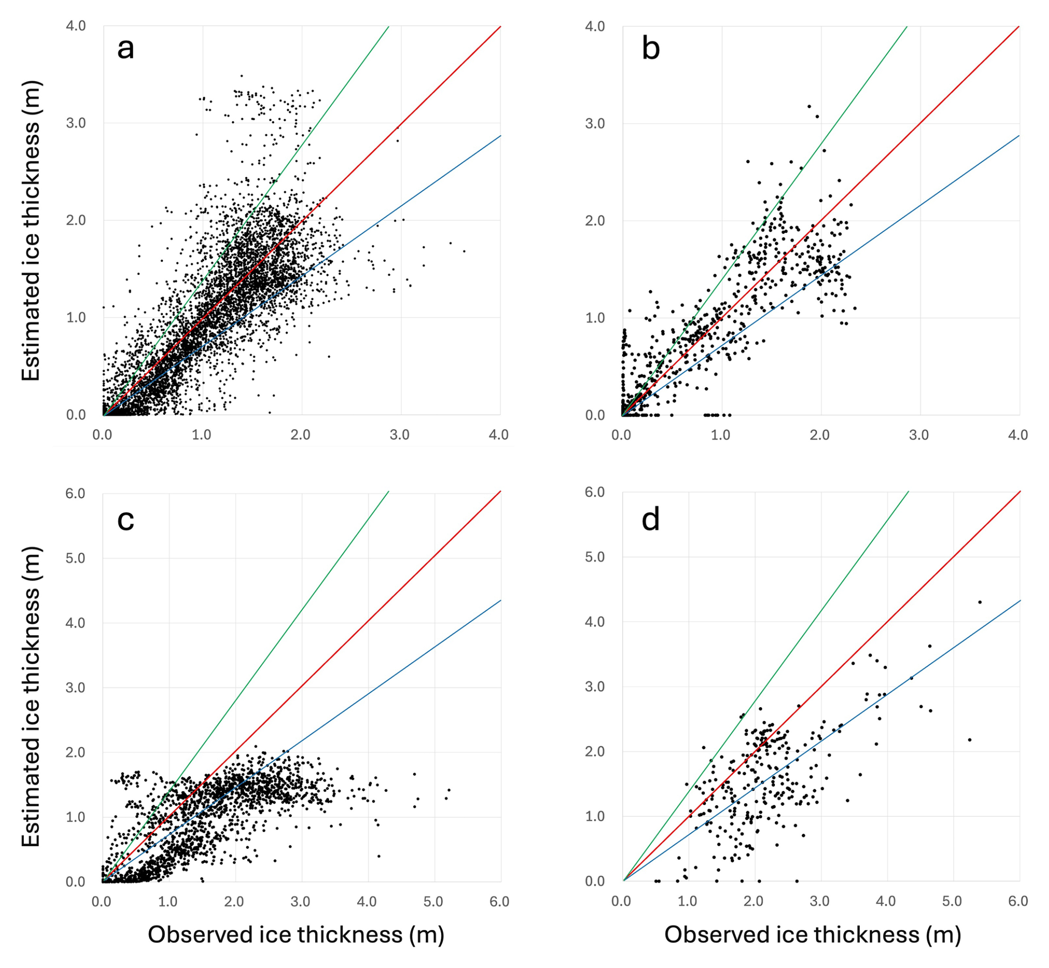
Figure 10 Scatter plots comparing the estimated sea ice thickness with observations from four different datasets. (a) Comparison with ULS observations in the Beaufort Sea (sites A, B, and D in Fig. 1a); (b) comparison with ULS observations in the Fram Strait (star in Fig. 1a); (c) comparison with ADCP observations in the Laptev Sea (red dot in Fig. 1a); and (d) comparison with EM observations (blue dot in Fig. 1a). The horizontal axes represent the observed ice thickness, and the vertical axes represent the corresponding estimated ice thickness. The red, blue, and green lines indicate results with scaling factors of 0.25, 0.35, and 0.15, respectively.

The scaling factor of 0.25 was then applied across the entire Northern Hemisphere to estimate the spatial distribution of sea ice thickness. Figure 11 illustrates the spatial distribution of estimated sea ice thickness on 31 May 2021. A prominent band of thick ice, exceeding 2.5 m and reaching over 3 m in the central regions, extends from the East Siberian Sea across the central Arctic Ocean toward the Canadian Arctic Archipelago. The Beaufort Sea and the region north of Greenland exhibit particularly thick ice, consistent with areas known for multiyear ice accumulation and limited summer melt. In contrast, thinner ice (less than 1 m) is widespread along the marginal seas of the Siberian side. This pattern resembles the distribution of older ice shown in Fig. 5b, but the spatial variation in ice thickness is more gradual than that of ice age. It also becomes apparent that areas with similar mean ice age do not necessarily have the same thickness.

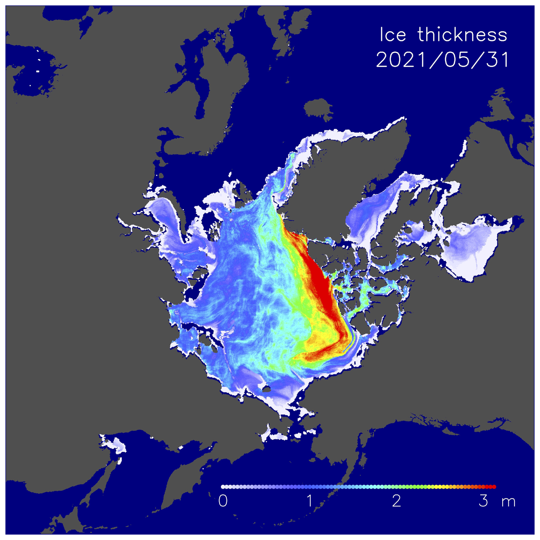
Figure 11 Estimated sea ice thickness on 31 May 2021. Thick ice is predominantly found along the northern coasts of the Canadian Arctic Archipelago and Greenland.

Figure 12 presents the monthly mean sea ice thickness for each month of 2021. Seasonal growth and decay patterns are clearly evident, with thickness gradually increasing from October through April, peaking in late spring, and subsequently declining through the summer months. The thickest ice, with maximum values exceeding 3 m, is observed in April and May, particularly along the Transpolar Drift Stream pathway and near the Canadian Arctic Archipelago. During summer (July–September), the spatial extent of thick ice contracts significantly, and overall ice thickness decreases, especially in marginal seas. Notably, even during the summer minimum, remnant thick ice persists in the central Arctic Ocean and north of the Canadian Basin. From October to December, new ice formation progresses, especially in the Siberian and Alaskan marginal seas, initiating the seasonal recovery of ice thickness.

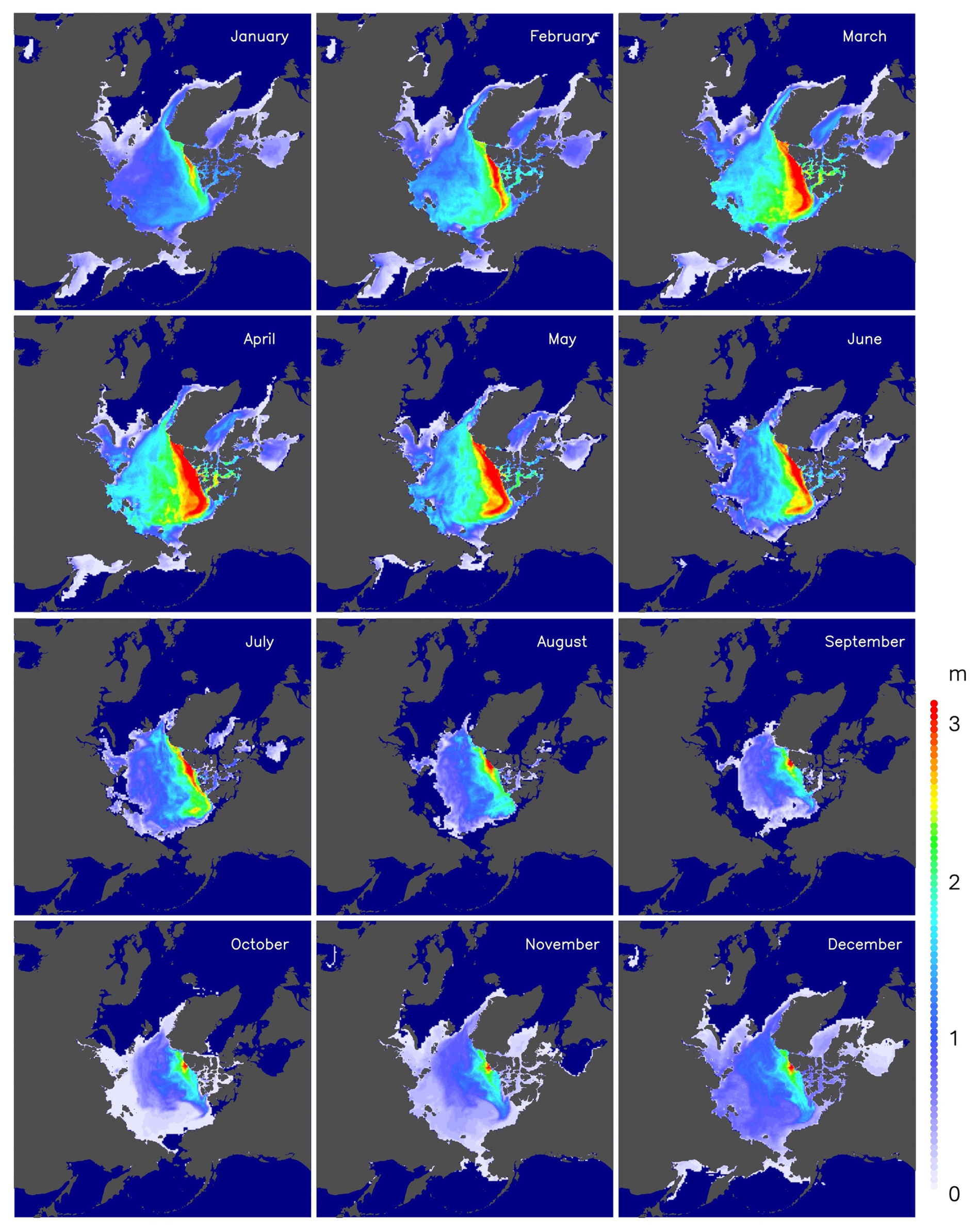
Figure 12 Monthly mean sea ice thickness for each month of 2021.

The daily sea ice thickness dataset developed here can be generated for the full AMSR-E and AMSR2 observational periods. Because the method requires up to four years of historical ice motion and concentration data, thickness cannot be calculated for the first four years after data acquisition begins. Accordingly, the dataset begins in 2007. However, due to the observational gap between the end of AMSR-E (October 2011) and the beginning of AMSR2 (July 2012), sea ice thickness data are also unavailable for the period between the end of AMSR-E (October 2011) and the point when sufficient AMSR2 history becomes available (July 2016).

5 Discussion

This study demonstrates that our method enables year-round estimation of sea ice thickness across the entire Northern Hemisphere. To evaluate whether these estimates are more reliable than existing datasets, we compared them with ULS observations from the Fram Strait – the same dataset used in Sect. 4. Importantly, these ULS data are not publicly available and are therefore not assimilated into currently available sea ice thickness products. Likewise, our estimates shown in Fig. 8 were generated without using these ULS observations, providing an independent benchmark for comparison.

Figure 13 compares the ULS observations with sea ice thickness estimates from PIOMAS and SMOS-CryoSat (ESA, 2023). The closest grid points to the mooring site were used for both datasets (11.8 km for PIOMAS and 10.0 km for SMOS-CryoSat). The PIOMAS data, available daily, capture the general seasonal pattern of sea ice growth and melt but fail to reproduce short-term fluctuations and tend to overestimate ice thickness during 2017–2018, thereby underrepresenting interannual contrast. SMOS-CryoSat provides weekly data but lacks coverage during the melt season, limiting its ability to represent the full seasonal cycle. It does, however, reflect the general year-to-year difference in ice thickness, distinguishing the thicker ice in 2016–2017 from the thinner ice in 2017–2018. These comparisons highlight the limitations of existing datasets in resolving fine-scale temporal variability and in providing continuous seasonal coverage.

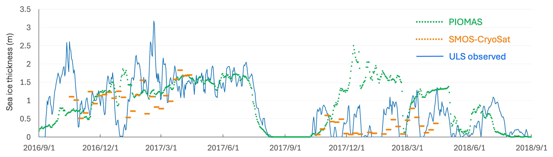
Figure 13 Comparison of the same ULS observations (blue line) with sea ice thickness from the PIOMAS reanalysis (green dots) and from the SMOS-CryoSat merged satellite product (orange dots). The SMOS-CryoSat data are based on weekly means.

In contrast, our estimates shown in Fig. 8 not only align well with direct ULS observations but also accurately reproduce short-term variability, seasonal evolution, and interannual differences. Furthermore, it provides year-round estimates from satellite data alone, overcoming the summertime coverage gap that affects other remote sensing methods such as SMOS-CryoSat, ICESat-2 (Petty et al., 2023), and passive microwave retrievals (e.g. AMSR; Krishfield et al., 2014). These capabilities highlight the value of our approach as a reliable and comprehensive tool for monitoring sea ice thickness across the Arctic.

A notable strength of the method is that it yields internally consistent sea ice thickness fields with limited sensitivity to short-term observational noise, ensuring stable spatial and temporal patterns throughout the year. This makes the data useful for applications such as initial conditions or data assimilation in numerical models.

However, our method does not resolve short-term (daily to sub-daily) variability because the input drift and concentration datasets have relatively coarse spatial resolution (∼ 60 km and ∼ 10 km). A more fundamental limitation is the omission of dynamic deformation processes such as ridging and rafting, which are known to contribute substantially to sea ice thickening (e.g. Leppäranta, 2011). These processes are not explicitly included in our estimates. As shown in Sect. 4, even though the mean thickness in the Beaufort Sea and Fram Strait agrees well with ULS observations, thickness is underestimated in the Laptev Sea, where dynamic deformation plays a much larger role in winter growth. While some caution is also warranted regarding the accuracy of thickness estimates derived from upward-looking ADCPs, Belter et al. (2021) demonstrated that the daily mean bias relative to ULS measurements is generally within about 20 %. Therefore, the underestimation found in our study is unlikely to be an artifact of the ADCP data themselves. Kimura et al. (2013) showed that winter–spring ice convergence strongly correlates with summer ice concentration in these regions, indicating that deformation-driven thickening is substantial and contributes to melt-resistant ice. The underestimation in our results likely reflects the absence of this process, and future versions of the dataset must incorporate dynamic deformation to fully capture ice growth in seasonal ice zones.

While Sect. 4 focused on mean ice thickness, Fig. 14 allows a comparison of the full seasonal evolution of the thickness distribution between ULS observations and our estimates. In our method, the distribution represents the spatial fraction of each thickness category, whereas in the ULS dataset it is derived from the frequency distribution of individual draft measurements (up to 86 400 samples per day). Despite this difference, both describe the thickness distribution over a given time period. Both datasets exhibit broadly similar seasonal cycles, with the prevalence of thicker ice increasing toward late spring and peaking between May and June. However, an important discrepancy is the scarcity of ice thicker than 4 m in our estimates, which is clearly present in the ULS observations. This difference likely reflects the influence of dynamic deformation processes that are absent from our thermodynamic-only framework. Deformation affects a wide range of thicknesses, but its signature is most apparent in the production of very thick ice. For example, von Albedyll et al. (2021) showed that dynamic processes contributed up to 90 % of the total ice thickness during the closure of a large polynya near northern Greenland in 2018. In our results, ice thicker than 3.5 m constituted 10 %–20 % of the area and contributed 30 %–60 % of the volume in winter, with a peak of nearly 80 % on 11 May 2019, implying that deformation influences the distribution more broadly than only at the thickest tail.

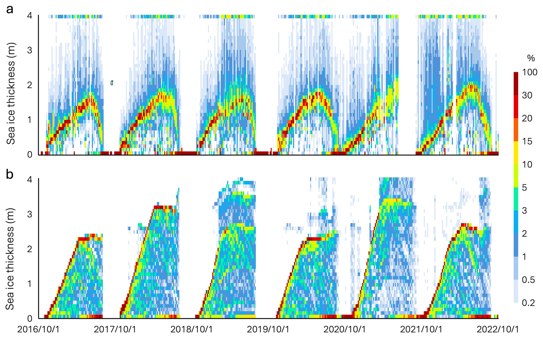
Figure 14 (a) Seasonal evolution of sea ice thickness distribution at mooring site A (location shown in Fig. 1a), shown for (a) ULS observations and (b) our estimates. The horizontal axis spans 1 October 2016 to 1 October 2022 at five-day resolution. The vertical axis shows ice thickness from 0 to 4 m, with ice thicker than 4 m included in the 4 m bin. Colors indicate the fractional contribution (%) of each 10 cm ice thickness category , with warmer colors representing higher percentages. This figure highlights how the distribution of thickness categories evolves through the seasons and allows direct comparison between observed and estimated thickness distribution.

Additional evidence of deformation effects appears in the evolution of modal thickness (highlighted in red in Fig. 14). In our estimates, the modal thickness increases almost linearly from autumn through winter because the open-water assumption produces a steady increase in growth potential. In contrast, the ULS observations show a progressively slower modal-thickness increase, consistent with the expected reduction in thermodynamic growth as the ice thickens, along with a growing fraction of ice thicker than the modal class, particularly ice exceeding 4 m. Despite these differences in distributional shape, the evolution of mean thickness agrees remarkably well between the two datasets (Fig. 7). This consistency can be explained by the structure of our method. Because the surface-flux–based growth potential is computed under open-water conditions throughout the growth season, the resulting cumulative growth tends to be larger than what would occur thermodynamically once the ice becomes thick. This systematic overestimation effectively offsets the missing contribution of dynamic deformation, which primarily enhances the thicker end of the distribution. As a result, although deformation is not represented explicitly, the combined effect allows our method to approximate the observed evolution of mean thickness and to implicitly incorporate both thermodynamic and dynamically induced thickening. Even though the open-water assumption allows partial compensation for dynamic thickening, this effect is insufficient in regions where deformation is strong. In the Laptev Sea, frequent occurrences of very thick ice are not fully captured by the method, causing the estimates to underestimate the largest peaks. This highlights the need for future improvements that explicitly incorporate dynamic thickening in such regions.

ULS data also show a smaller fraction of thin ice compared to our estimates. Two mechanisms may explain this: (1) thinner ice is more susceptible to deformation and subsequent thickening (Melling and Riedel, 1996), and (2) in our estimation, daily area loss is distributed uniformly across thickness categories, whereas in reality, thinner ice tends to melt and disappear more easily. These discrepancies show the importance of refining both thermodynamic and dynamic processes in future efforts.

An important source of uncertainty in the present method arises from the simplified representation of ice growth and the use of a constant scaling factor to convert accumulated thermodynamic growth into ice thickness. This scaling factor should not be interpreted purely as an empirical correction, but rather as an effective parameter that implicitly represents processes not explicitly included in the model, particularly dynamic deformation such as ridging and rafting, as well as uncertainties in the applied heat budget. If dynamic deformation were explicitly incorporated using deformation-related history such as convergence and shear along ice trajectories, the total thickness could be expressed as the sum of thermodynamic and dynamically induced contributions, each with its own proportionality factor. In such a framework, the proportionality factor associated with thermodynamic growth alone would likely be smaller than the current value of 0.25. However, constraining these contributions separately requires additional observational and process-based analyses and is beyond the scope of the present study. Nevertheless, the close agreement between our estimates and independent observations suggests that, on average, dynamically induced thickening scales approximately with thermodynamic growth, allowing realistic thickness to be derived within a simplified, observation-based framework. This interpretation provides a useful basis for further development of process-resolving thickness estimates and offers insight into the effective relationship between thermodynamic forcing and total ice thickness.

6 Summary

This study presented a new method for estimating Arctic sea ice thickness by reconstructing the thermodynamic growth history of individual ice parcels from satellite-derived ice motion and concentration data. The resulting thickness estimates reproduce the observed seasonal and interannual variability recorded by ULS moorings in both the Beaufort Sea and the Fram Strait, with RMS errors of 44.0 and 36.3 cm, respectively. Unlike existing satellite-based thickness products, the method provides spatially and temporally continuous estimates throughout the entire year, thereby bridging the summertime observational gap and enabling consistent monitoring across the Arctic Basin.

By assuming growth under open-water thermodynamic conditions, the approach offers a unified, observation-based framework that captures the cumulative effects of the surface heat budget along each parcel's drift history. The resulting thickness distributions exhibit realistic seasonal evolution and spatial patterns broadly consistent with known multiyear-ice characteristics. However, evaluation in the Laptev Sea highlights an important limitation: in regions where dynamic deformation processes such as ridging and rafting contribute substantially to winter growth, the method tends to underestimate total ice thickness because these processes are not explicitly represented.

Future developments will focus on incorporating deformation-related thickening into the framework and on extending the approach to reproduce the full seasonal evolution of the thickness distribution, not only its mean. It should be emphasized that the primary objective of this study is to estimate sea ice thickness based on ice history, rather than to explicitly resolve individual growth processes such as formation in polynyas or leads. Nevertheless, incorporating deformation history and more realistic thermodynamic growth formulations will enable a more process-based and physically complete representation of sea ice thickness evolution. Overall, the trajectory-based reconstruction of sea ice growth histories provides a promising pathway for generating long-term, observation-driven sea ice thickness datasets and for improving assessments of the changing Arctic ice cover.

Beyond its application to ice thickness, the present results demonstrate the broader potential of history-based approaches in sea ice remote sensing. By linking satellite-derived ice histories to physical properties observed in situ, the method shifts the focus from instantaneous snapshots to the temporal evolution of individual ice parcels. This opens new avenues for retrieving key sea ice characteristics that have historically been considered inaccessible, such as floe size distribution, melt pond evolution, or other dynamical and thermodynamical indicators tied to the life cycle of the ice. In this sense, the framework represents a step change in sea ice monitoring, illustrating how physically informed use of satellite data can expand our capability to observe and understand the rapidly evolving ice cover.