Effects of subgrid-scale ice topography on the ice shelf basal melting simulated in NEMO-4.2.0

At the interface between the ocean and the ice shelf base, in the framework of the shear-controlled melt parameterisation, the ice melts due to combined actions of temperature, salinity and friction velocity. In the NEMO ocean model, the friction velocity is usually computed based on a constant drag coefficient and an ocean velocity averaged vertically within a distance from the ice, which is often referred to as the Losch layer. Instead, in this study, we use a logarithmic approach, where a constant hydrographic roughness length detetermines the drag coefficient through the law of the wall and the horizontal current speed is sampled in the first wet cell. The aim is to reduce the vertical resolution dependency, to homogeneise the sampling of horizontal current speed between the thermodynamic and the dynamic drag equation and to enable the use of a variable drag coefficient based on the subgrid-scale (or unresolved) ice shelf basal topography. The motivation behind a variable drag based on the topography comes from observations showing that regions with rough topographic features such as crevasses or basal melt channels experience more melts than flat ones. We compare different experiments in a configuration of the Amundsen Sea at $\mathrm{1}/\mathrm{12}$°. We find that our approach is less sensitive (6 % melt rates difference) to a coarser vertical resolution, such as the one used in global Earth System Models, than the Losch layer approach (22 % melt rates difference). We also find that it succeeds in reproducing higher melt rates in rougher regions while keeping total ice shelf melt rate within the observed range. Finally, to assess the effect of increasing ice shelf damage, we tested the sensitivity of a higher hydrographic roughness length. If the roughness of all the ice shelf grid points were to increase to the highest value currently observed, the overall ice shelf melting would increase by 16 %. This suggests the possibility of a positive feedback in which more melting leads to more ice damage and increased roughness, in turn increasing melt rates.

1 Introduction

Around most of Antarctica, the margins of the ice sheet form floating ice shelves, a safety band buttressing continental ice (Fürst et al., 2016; Reese et al., 2018) and limiting the ice flow (Pegler, 2018). They are crucial to ice sheet stability and many of them are currently losing mass, which, in turn, has direct consequences on the whole ice sheet mass loss (Paolo et al., 2015; Gudmundsson et al., 2019; Joughin et al., 2021; Davison et al., 2023; Miles and Bingham, 2024). Eventually the resulting weakening of ice shelves will have global consequences on climate (Bronselaer et al., 2018) and sea level rise (Sun et al., 2020; Edwards et al., 2021; Seroussi et al., 2024) but before collapsing, ice shelves may gradually build damage through an intensification of surface and basal crevasses (Lhermitte et al., 2020) related to ice velocity changes (Surawy-Stepney et al., 2023). Ultimately, ice shelves could potentially enter a disintegrated state where the ice is broken up and composed of ice mélange currently observed for the Thwaites Glacier Tongue, Amundsen Sea (Joughin et al., 2014; Miles et al., 2020).

At the same time, half of the mass loss from ice shelves is attributable to sub-shelf melting due to ocean forcing (Depoorter et al., 2013), which has accelerated over the last decades, mainly in the Amundsen-Bellingshausen sector (Davison et al., 2023). Warmer and saltier waters, transported through the turbulent ice shelf-ocean boundary layer to the ice by vertical mixing could potentially induce more melting and the resulting new geometry could lead to different melting patterns (Dutrieux et al., 2016; Donat-Magnin et al., 2017; Holland et al., 2023; De Rydt and Naughten, 2024).

Below ice shelves, the ice is rough at various scales and melt rates are related to ice roughness to a certain extent (Watkins et al., 2021; Larter, 2022; Bassis et al., 2024). From large features such as basal channels (Gourmelen et al., 2017; Alley et al., 2023), rifts (Orheim et al., 1990), terrasses (Dutrieux et al., 2014) or basal crevasses (McGrath et al., 2012) to small scale features such as scallops, runnels or marine ice facies (Schmidt et al., 2023; Washam et al., 2023; Wåhlin et al., 2024), observations show enhanced melting in rougher ice regions. Flat features like terrasses present lower melt rates than steep features like crevasses (Davis et al., 2023; Schmidt et al., 2023; Wåhlin et al., 2024).

Some attempts of studying the impact of a crevasse (Jordan et al., 2014), a rift (Poinelli et al., 2023) or a basal channel (Zhou and Hattermann, 2020), with high resolution models, showed their influence on the circulation. Nakayama et al. (2019), in a study in the Amundsen Sea Embayment (ASE), emphasized the need for accurate and high resolution topographies (top and bottom) in order to determine ocean pathways and melt patterns, which are particularly sensitive to ocean velocity (and to a larger extent friction velocity) near the ice base. However, in current ocean models, if the feature is not resolved, there is no distinction between smooth and rough areas. A way to take roughness into account is to parameterise subgrid drag processes.

At the interface between the ice and the ocean, shear typically creates an ice–ocean boundary layer beneath the ice which can be divided into an inner layer and an outer layer dominated by turbulent fluxes (see Fig. 1). In the vicinity of the interface, the inner layer comprises the viscous sublayer and the logarithmic sublayer with a combined thickness of a few meters.

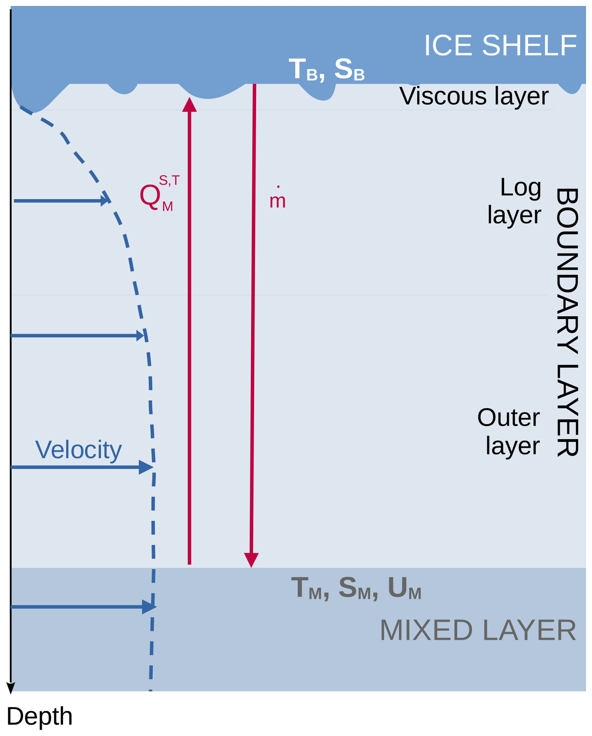
Figure 1 Sketch of the boundary layer at the interface between the ice and the ocean below ice shelves assuming a well-mixed shear controlled turbulence regime.

Thermodynamic exchanges at the interface between the ocean and the ice are usually parameterised using the three-equation parameterisation (Holland and Jenkins, 1999), also referred to as the shear-controlled melting parameterisation (see Appendix A) where the friction velocity, $u_{*}=C_{\mathrm{d}}{U}_{\mathrm{M}}^{\mathrm{2}}$, is usually formulated as a quadratic drag parameterisation of the mean horizontal current speed, U_M, sampled at a certain distance from the ice and using a drag coefficient, C_d. Although this melt parameterisation proved to perform properly in some cases, we note one important and known caveat (among others): the drag parameterisation. The boundary layer depth can be represented by the top cell (or first wet cell) thickness. This leads to a strong dependency on vertical resolution (Gwyther et al., 2020; Patmore et al., 2023; Burchard et al., 2022). Some models, particularly z coordinate models, empirically define a constant boundary layer depth over which mean tracers are averaged to calculate melt rates as first proposed by Losch (2008). They defined this layer, sometimes referred to as the Losch layer, as the thickness of a single full grid cell, so that even with partial steps, the same thickness was used for all cells. They used the original ISOMIP configuration, which has a uniform nominal resolution of 30 m for all levels. In contrast, most realistic configurations make use of a non-uniform vertical resolution. It means that the deepest parts of ice shelf cavities have a coarser vertical grid than the parts closer to the sea surface. To remove noise, as proposed by Losch (2008), a Losch layer of 30 m may span several cells. However, the choice of the Losch layer thickness is not physically based and has an impact on the results (Mathiot et al., 2017).

Modellers would generally tune their model parameters, such as C_d, to fit observations. Different models and configurations may use different tuning parameters for the same result, with certainly different sensitivities to ocean forcing and/or geometry in a changing climate leading to potentially different results and large uncertainties.

It is therefore important to better parameterise mechanisms implied in the ice–ocean boundary layer where vertical shear forms and where melt depends on the friction velocity, u_*. In the vicinity of the interface, in the logarithmic sublayer (below the viscous layer), it is common to use the “law of the wall” (valid under neutral conditions) to describe the velocity profile (McPhee et al., 2008), U(z), as

$$\begin{array}{}\text{(1)}& U\left(z\right)={\displaystyle \frac{u_{*}}{\mathit{\kappa }}}\ln \left({\displaystyle \frac{z}{z_{\mathrm{0}}}}\right)\end{array}$$

where κ=0.4 is the von Kármán's constant and z₀, the hydrographic roughness length, the height (or depth) at which the speed theoretically becomes zero under neutral conditions.

Optimally, C_d should be able to vary in space and time (Davis and Nicholls, 2019; Vreugdenhil and Taylor, 2019; Rosevear et al., 2022), be independent of vertical resolution (Patmore et al., 2023) and be more physically-grounded. Besides, Gwyther et al. (2020) suggested that the use of a constant and tuned C_d may not be consistent with sampling or averaging locations. To reduce the vertical dependency, Burchard et al. (2022) suggested to use Eq. (1) so that C_d is at least a function of vertical resolution although Patmore et al. (2023) reported negligible effects. Using a varying C_d in space in time and has been explored at other interfaces. For instance, the momentum of the atmosphere is influenced by the subgrid scale orography (Lott and Miller, 1997). Jourdain and Gallée (2011) found that katabatic winds of wide valleys in the Transantarctic Mountains were very sensitive to the orographic roughness. Hughes (2022) used this parameterisation to conceptualise ocean currents passing through an idealised ice mélange. McPhee (2012) presented a formulation of the drag law at the sea ice/ocean interface explicitely accounting for variation of hydrographic roughness length and buoyancy flux. Steiner (2001), Tsamados et al. (2014) and Lu et al. (2011) estimated the total drag as a combination of form drag and skin drag depending on either the deformation energy or the statistical obstacle geometry and the ice concentration. To our knowledge, under ice shelves, only Gwyther et al. (2015) led a series of experiments with varying C_d, depending on the melting or freezing state of the ice.

In the present study, we propose to investigate the use of the law of the wall (Eq. 1) with a constant hydrographic roughness length or a spatially varying “topographic roughness” depending on the sub-shelf topography. We use a regional configuration of NEMO4.2 in the Amundsen Sea with open cavities (Mathiot et al., 2017; Jourdain et al., 2017) and compare this new approach to the Losch layer approach.

2 Simulations and experiments

2.1 Ocean model, configuration and observational Data

In this study we use the three-dimensional, free-surface, hydrostatic, primitive-equation global ocean general circulation model NEMO version 4.2 (Madec et al., 2022). This model includes a sea ice module as well as an ice shelf cavity module (Mathiot et al., 2017). The model is discretized on an Arakawa C-type grid where different variables are solved at different places on a 3D-grid cell (see Fig. 2a). For instance, temperature and salinity are computed at the centre of the cell (T-point or coordinate indices i,j) and the x-ward and y-ward velocity components, u and v, are computed at the cell boundaries (U-point of coordinate indices $i+\mathrm{1}/\mathrm{2},j$ for u, and V-point of coordinates $i,j+\mathrm{1}/\mathrm{2}$ for v).

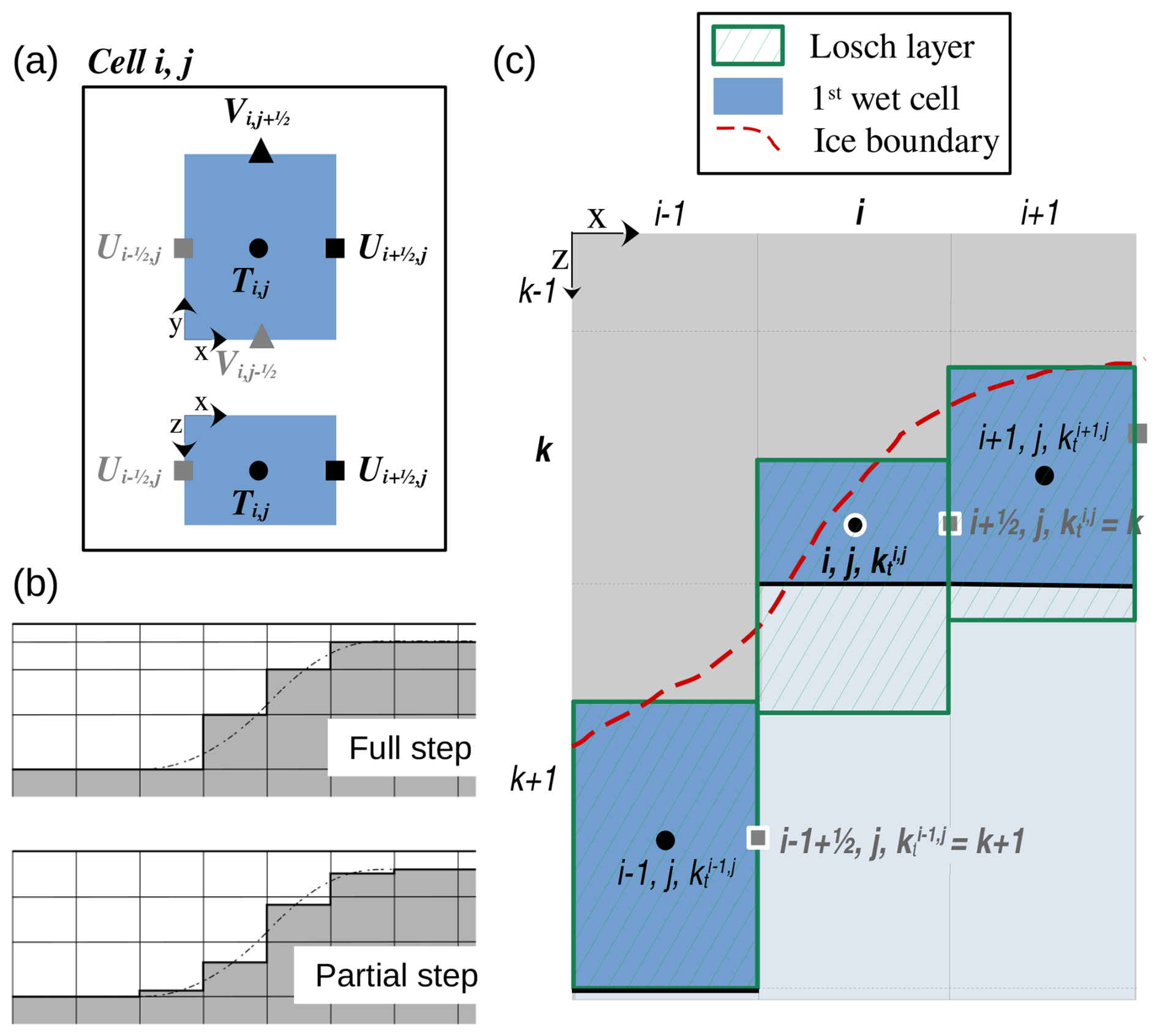
Figure 2 (a) Arakawa C-type grid cell (i,j) in x-y coordinates and x-z coordinates is shown with T-, U- and V-points. (b) z coordinate systems with full step and with partial step at the surface (adapted from Madec et al., 2022). (c) Sketch of partial step z^* coordinate grid showing the ice shelf in grey (deactivated cells) and the ocean in light blue in x-z coordinates. The first wet cell under the ice shelf is colored in dark blue and the Losch layer is hatched in green. The losch layer is always thicker or equal to the first wet cell thickness. The red line represents the ice–ocean boundary as in high resolution data.

2.1.1 Amundsen Sea Embayment configuration and simulations

Our Amundsen Sea configuration (Fig. 3), has a resolution of $\mathrm{1}/\mathrm{12}$° with a grid extending from 142.1 to 84.9° W and from 76.5 to 59.7° S similar to the one used in Jourdain et al. (2022) but with 121 vertical levels instead of 75 (more details are given in Sect. 2.1.2). The lateral ocean and sea ice boundary conditions as well as melt rates from iceberg melting are extracted from 5 d mean outputs of a global 0.25° NEMO simulation, representing Lagrangian icebergs (Mathiot and Jourdain, 2023). Seven constituents of the barotropic tides are prescribed at the lateral boundaries (Jourdain et al., 2019).

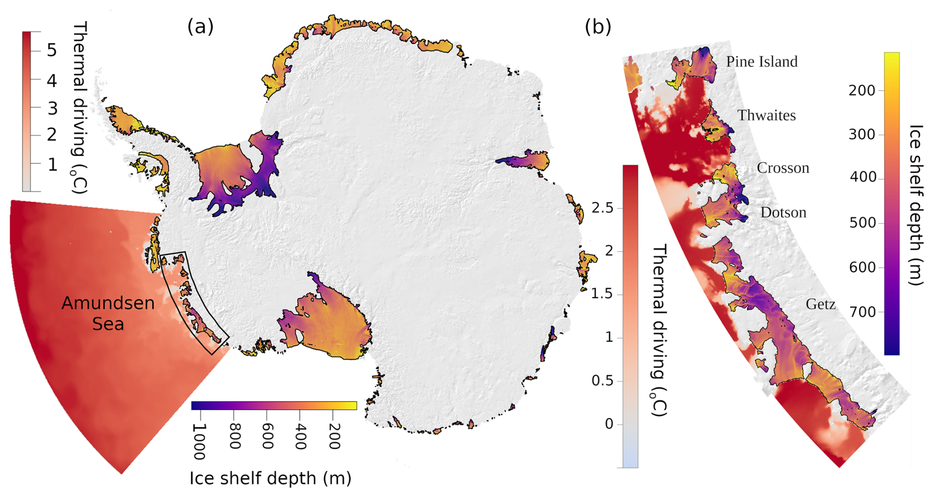
Figure 3 (a) Amundsen Sea configuration domain in Antarctica and (b) zoom on the studied ice shelves. Ice is shown with grayscale of the hillshade to emphasize the rough environment. Ice Shelf colormap represents basal topography (BedMachine Antarctica v2 from Morlighem et al., 2019) and ocean colormap represents the thermal driving mean between 200 and 800 m (from reference experiment).

Simulations start in 2005 from the global 0.25° NEMO simulation ocean conditions and are spun-up until 2010. Each configuration is then run from 2010–2013. Results presented in this study are a temporal average of year 2013.

2.1.2 Vertical coordinate system and resolution

We use a curvilinear z^* coordinate system with partial steps to adjust the thickness of grid cells adjacent to the sea floor (bottom level and index k_b) or ice shelf draft (top level and index k_t) in order to simulate a realistic water column thickness. Therefore, the cell thickness near the sea floor and ice-shelf draft depend not only on the k vertical grid index, but also on the horizontal i,j indices. This allows a realistic water column thickness everywhere. Beneath the ice shelf, we note $e_{\mathrm{3}}^{i,j,k_{\mathrm{t}}}$ the thickness of the first wet cell (level k_t) of the horizontal grid cell i,j after partial stepping. The subscript 3 refers to the vertical component while 1 and 2 refer to the horizontal ones. Figure 2b and c show the partial cell treatment of the first wet cell (just below the ice) and Fig. 4 shows the first wet cell thickness for ice shelves in the ASE. Ice shelf drafts in the ASE are typically spanning between 100–1000 m depth, and we use 121 vertical levels defined as in Mathiot and Jourdain (2023), with a fairly constant vertical nominal resolution (before partial stepping) between 100 and 1000 m (level thickness around 10–20 m) as shown in Fig. 5 and Table 1.

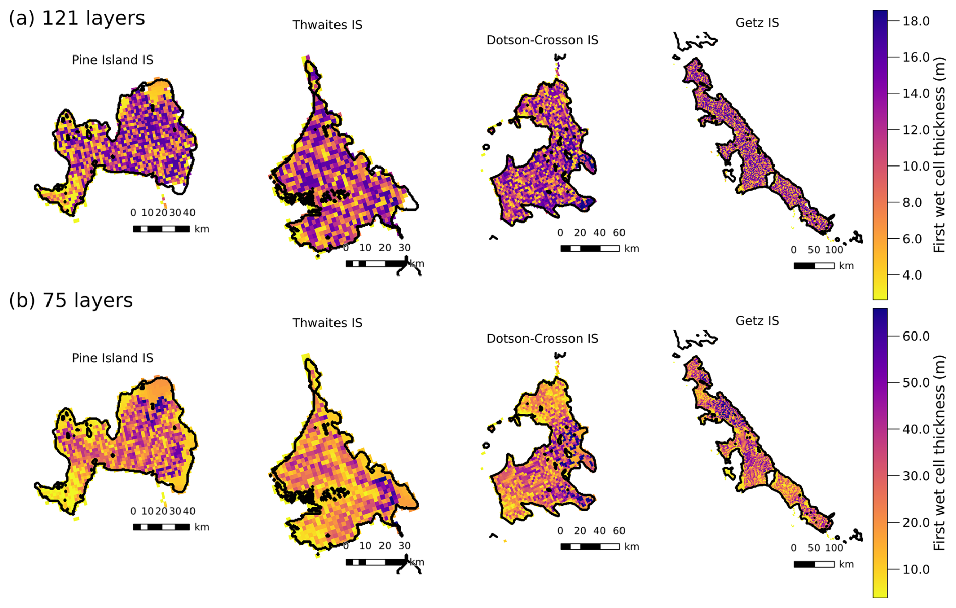
Figure 4 First wet cell height below ice shelves in the ASE configuration with (a) 121 layers and (b) 75 layers.

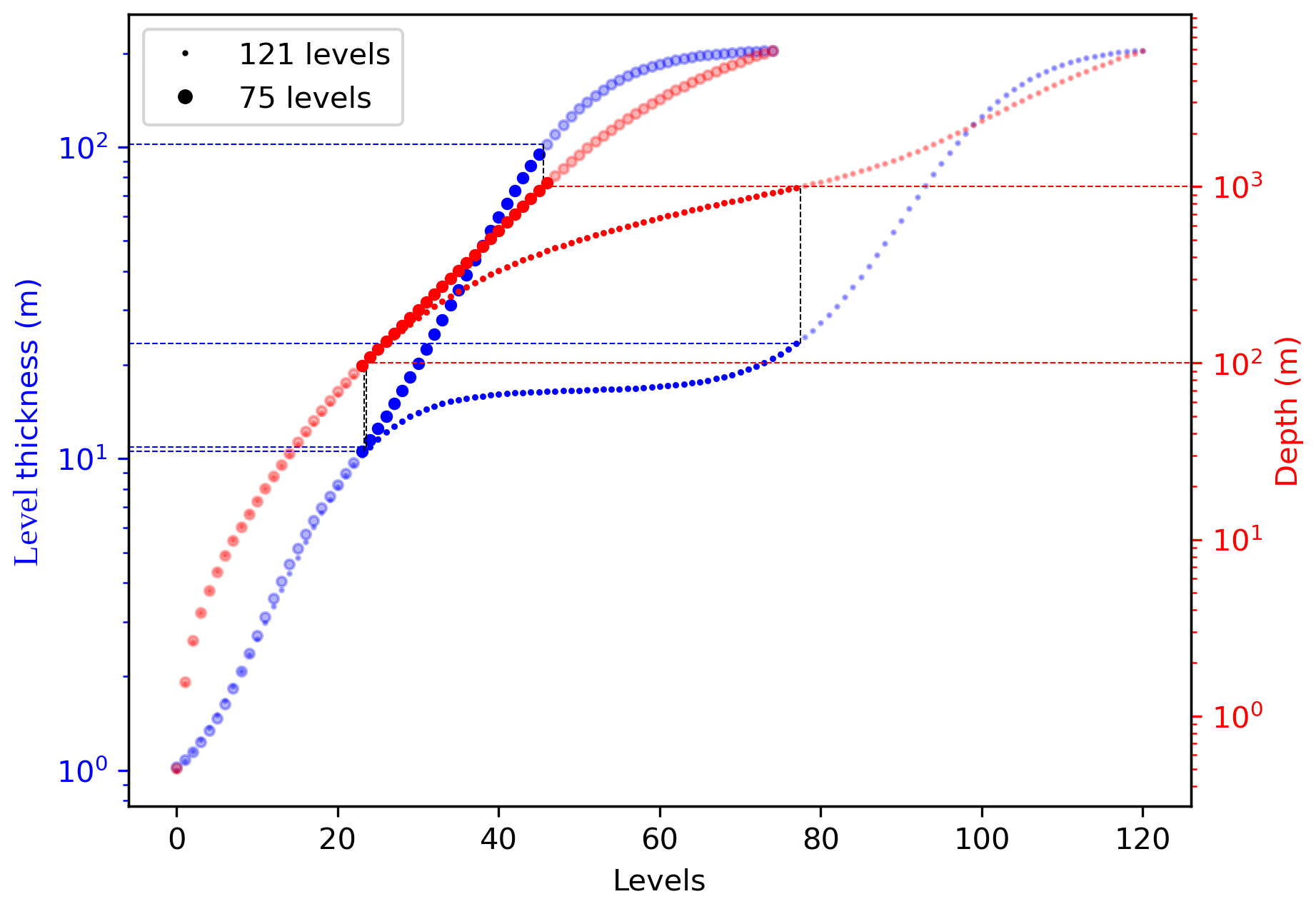
Figure 5 Vertical cell thickness in m (blue) and depth in m (red) as a function of levels for 121 levels (small dots) and 75 levels (big dots). Red horizontal dashed lines show 100 and 1000 m depth. Vertical black lines mark the level thickness at 100 and 1000 m depth for both 121 and 75 levels. Blue horizontal dashed lines match the 100 and 1000 m depth limits level thickness counterparts.

Table 1 Level thickness for 121 and 75 vertical levels in function of depth.

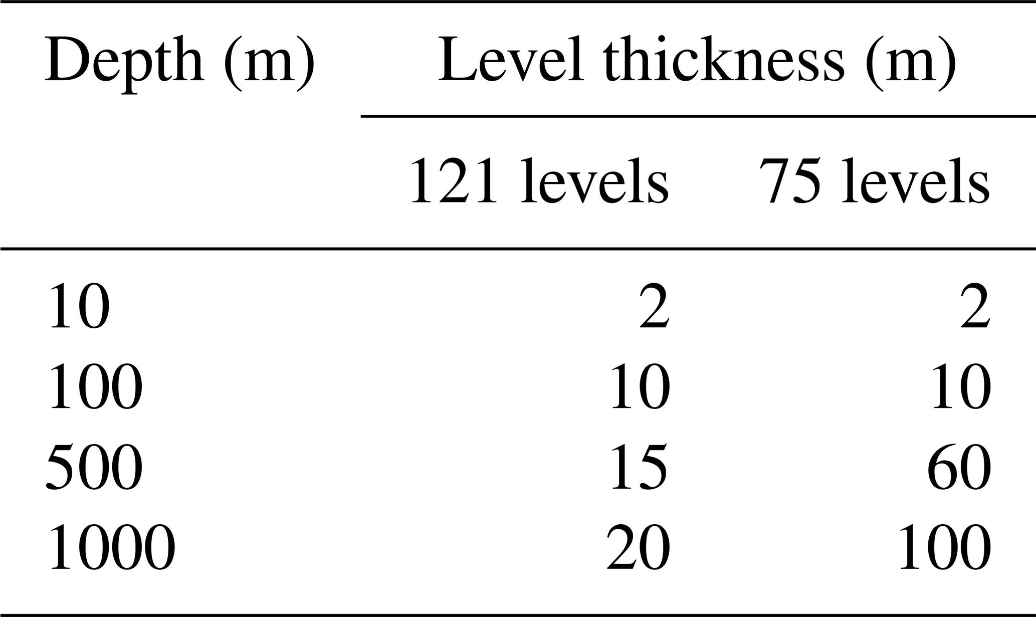
To test the sensitivity to the vertical resolution, we also use a configuration with 75 levels (as used in standard global Earth System Models) where the level thickness between 100–1000 m is between 10–100 m (see curves marked by large dots in plain colors in Fig. 5 and Table 1). Depending on the verical resolution, ice shelves in ASE have one or more cells in the Losch layer (Fig. 6a) with important differences in the sum of cells thicknesses (Fig. 6b).

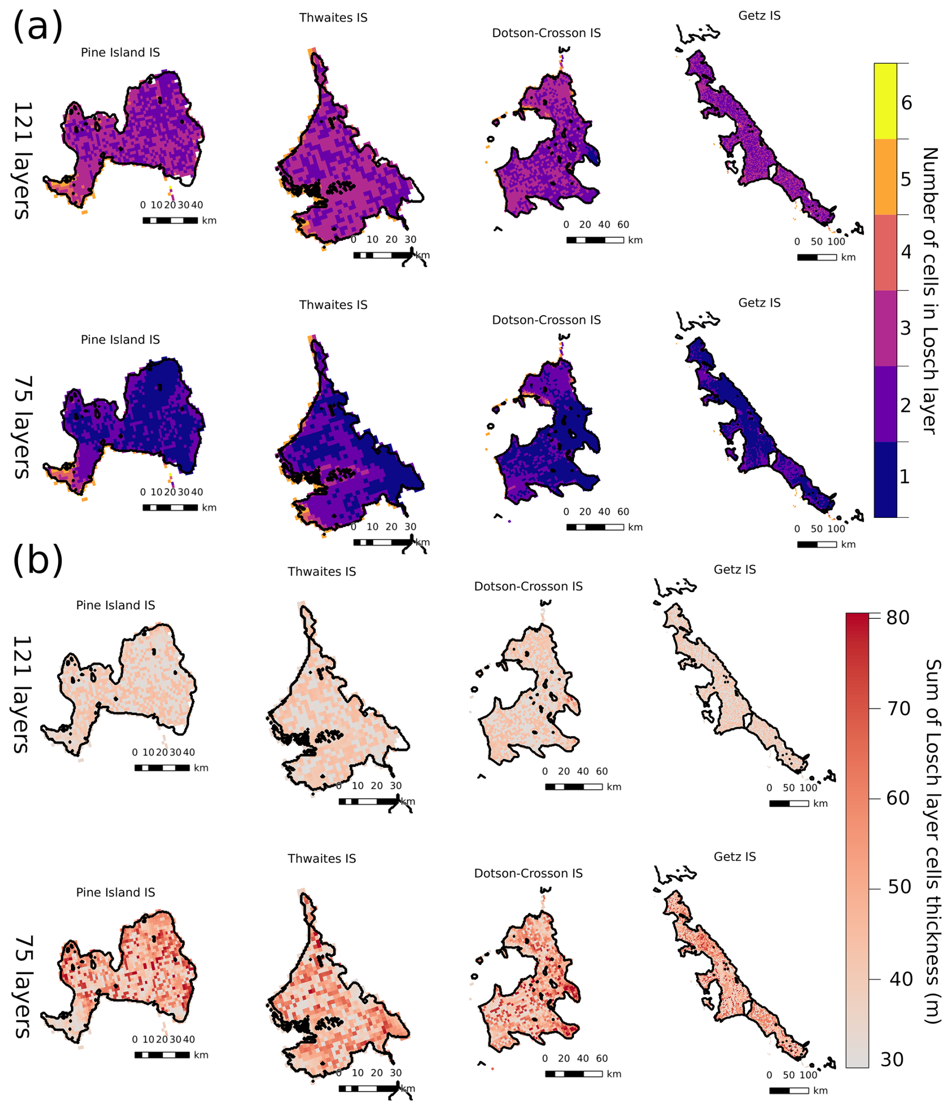
Figure 6 (a) Number of cells included in a 30 m thick Losch layer for 121 and 75 levels. (b) Sum of full cell thicknesses contained in the Losch layer for 121 and 75 levels. Note that if the Losch layer is thicker than the first wet cell, the velocity of the last cell is scaled to the fraction left. Otherwise it is the first wet cell velocity.

2.1.3 Observational data

We use the Japanese 55 year reanalysis (JRA-55-do), a 3 h high resolution atmospheric reanalysis provided by the Japan Meteorology Agency (Tsujino et al., 2018) for the surface boundary conditions (air temperature, humidity, wind velocity, radiative fluxes and precipitation).

The ice shelf draft and bathymetry is taken from the BedMachine Antarctica v2 (Morlighem et al., 2019). This is a dataset on a 500 m resolution grid of the Antarctic ice sheet and the surrounding ocean using data from 1993–2016 with a nominal date of 2012. It provides a mask with ice free land, grounded ice, floating ice and ocean, a bed topography collected from different sources, a surface elevation from the Reference Elevation Model of Antarctica (REMA) described in the section below (Howat et al., 2022), an ice thickness (inferred from mass conservation along the periphery of the ice sheet) and an error map.

To calculate the “topographic roughness”, R, at the base of the ice shelf, we use a simple definition: the largest inter-cell difference between a pixel value and its adjacent cells (Wilson et al., 2007). In other words, at the location of each pixel, the largest difference between its 8 neighbours is chosen. We chose this method for its simplicity and its correlation with the maximum slope. Other methods are discussed in Sect. 3.6. Thereafter, we use a conservative regridding method for which the weight calculation is based on the ratio of source cell area overlapped with the corresponding destination cell area.

To assess the sensitivity of our roughness estimates, we use several topography datasets of various resolution:

• 500 m from BedMachine Antarctica v2 (Morlighem et al., 2019)

• 100 m from REMA v2.0 (Howat et al., 2022)

• 32 m from REMA v2.0 (Howat et al., 2022)

The REMA dataset is a high resolution terrain map of Antarctica constructed from stereoscopic Digital Elevation Models (DEM) acquired between 2009 and 2021 and referenced to the WGS84 ellipsoid. They provide Strip and mosaic DEM files at different resolutions. We followed Bevan et al. (2021), to adjust the surface elevation and to calculate the ice shelf thickness assuming hydrostatic equilibrium.

2.1.4 Classical drag parameterisation: the Losch layer approach (REF)

Beneath ice shelves, the vertical shear stress, τ, related to the friction velocity, u_*, is associated with both dynamic flow over rough surfaces and thermodynamic exchanges between the ice and the ocean (Eqs. A1–A3 in Appendix A). In NEMO, we usually use a quadratic parameterisation to relate the friction velocity, u_* to the horizontal current speed, U_M with a constant and dimensionless drag coefficient, C_d,

$$\begin{array}{}\text{(2)}& u_{*}^{\mathrm{2}}=C_{\mathrm{d}}{U}_{\mathrm{M}}^{\mathrm{2}}\end{array}$$

The mean horizontal current speed, U_M, is computed in the first wet cell to solve the momentum equations. To solve the thermodynamic equations, to limit the dependency to vertical resolution and facilitate the upward density flow along stair cases, we use a weighted average of the velocity over the Losch layer thickness (usually 30 m) (Losch, 2008). The weighted average is computed between the top of the first wet cell and the fraction of the bottom cell of the Losch layer. If the first wet cell thickness is thicker than the Losch layer thickness, we use the first wet cell velocity. Examples of Losch layer configurations are represented in Fig. 2c and more details are presented in Appendix B1.

2.2 Proposed drag parameterisation: the logarithmic approach (LOG) and the “topographic roughness” approach (ROUGH)

We propose to homogenise the treatment of shear by solving the friction velocity in the first wet cell in both the dynamic and the thermodynamic equations, and to reduce the dependence of the drag coefficient in z by using the law of the wall (Eq. 1). From Eqs. (2) and (1), C_d takes the form

$$\begin{array}{}\text{(3)}& C_{\mathrm{d}}={\left({\displaystyle \frac{\mathit{\kappa }}{\ln \frac{z}{z_{\mathrm{0}}}}}\right)}^{\mathrm{2}}\end{array}$$

with z, half of the first wet cell thickness and z₀, the hydrographic roughness length. In the logarithmic approach (LOG) case, z₀ is constant everywhere while C_d is z-dependent. In the “topographic roughness” approach (ROUGH) case, z₀ is given at T-point. The friction velocity, u_* and the hydrographic roughness length (in the ROUGH case) are calculated at T-point, while velocity components (u,v) are computed at U- and V-point respectively. Since the difference between neighbouring cell thicknesses can be non negligible, particularly in the coarser cases (see Fig. 4b), we need to linearly interpolate C_d in between two cells and calculate the resulting u_* at U-point $(i+\frac{\mathrm{1}}{\mathrm{2}},j,k_{\mathrm{t}}^{i,j})$ and V-point $(i,j+\frac{\mathrm{1}}{\mathrm{2}},k_{\mathrm{t}}^{i,j})$ respectively and take the mean at T-point. More details are given in Appendix B2. The sketch of Fig. 2a shows the difference between the treatment on the first wet cell and on the Losch layer for z^* coordinate system with partial steps.

The choice of z₀ is of course important as shown in Fig. 7a. Likewise, it is important to note the difference of C_d given the cell height (2–18 m for L121 and 2–60 m for L75). For $z_{\mathrm{0}}=\mathrm{3}\times {\mathrm{10}}^{-\mathrm{4}}$ m, $C_{\mathrm{d}}=\mathrm{2.5}\times {\mathrm{10}}^{-\mathrm{3}}$ at z=1 m, $C_{\mathrm{d}}=\mathrm{2}\times {\mathrm{10}}^{-\mathrm{3}}$ at z=2 m and $C_{\mathrm{d}}=\mathrm{1.5}\times {\mathrm{10}}^{-\mathrm{3}}$ at z=15 m from the ice interface. This means that the change between 1 and 2 m is as large as the change between 2 and 15 m. This also means that, at high resolution, this formulation has important effects. These values of C_d are expected to lead to significantly different melt rates (see Fig. 6 of Jourdain et al., 2017), and this range of z values is common due to the use of partial cells and to the fact that fields are usually calculated at the cell centers (i.e., z is half the cell thickness). To make sure the difference between the two parameterisations is not only dependent on the choice of the first wet cell, we propose an experiment with a constant drag on the first wet cell.

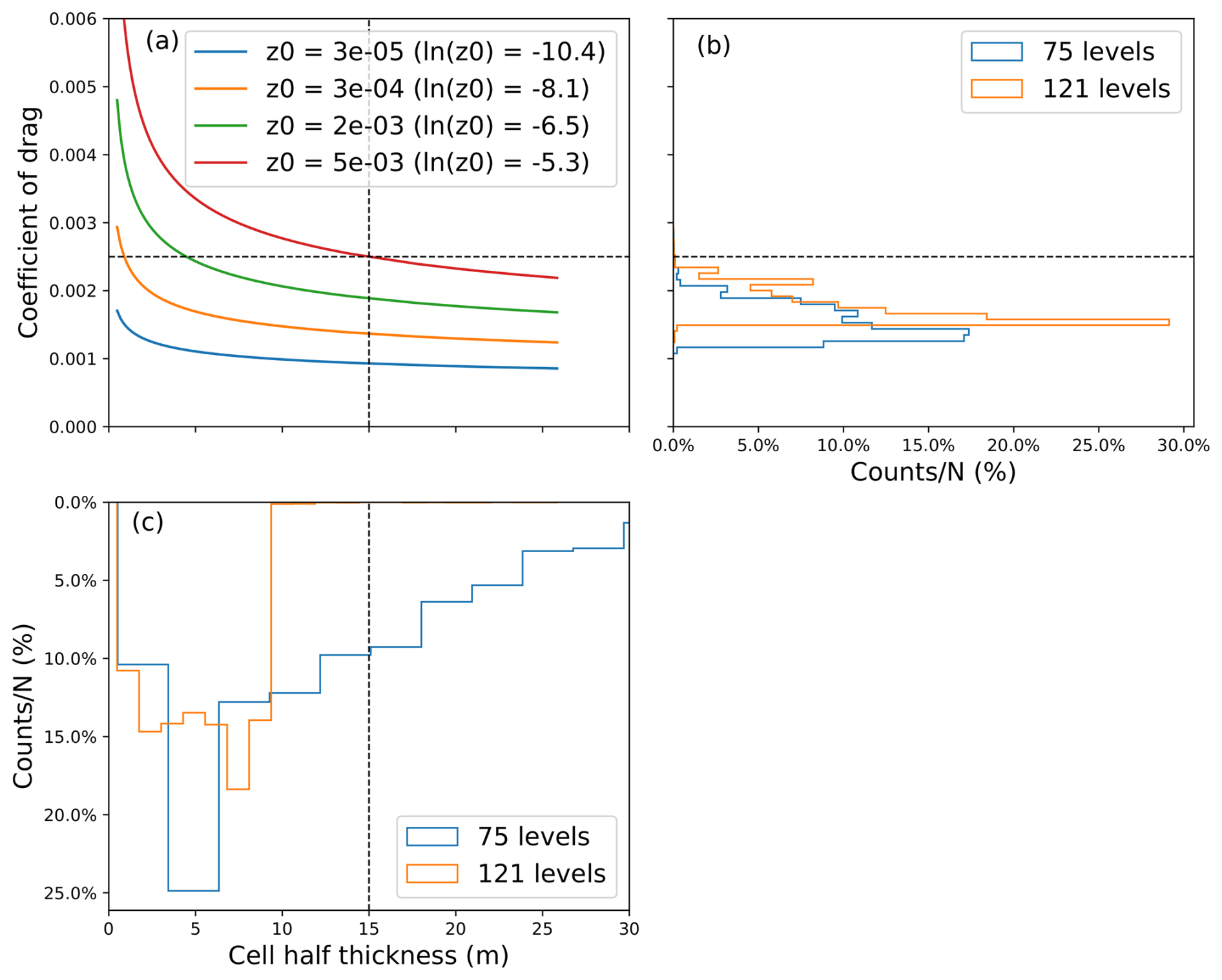
Figure 7 (a) Drag coefficient following the law of the wall for four different z₀. The horizontal dashed line represents a drag coefficient of $\mathrm{2.5}\times {\mathrm{10}}^{-\mathrm{3}}$ and the vertical dashed line represents a cell helf thickness of 15 m (cell thickness of 30 m). (b) Histograms of drag coefficient for $z_{\mathrm{0}}=\mathrm{3}\times {\mathrm{10}}^{-\mathrm{4}}$ m for 75 levels (blue) and 121 levels (orange) for all ice shelves. (c) Histograms of cell half thickness (m) for $z_{\mathrm{0}}=\mathrm{3}\times {\mathrm{10}}^{-\mathrm{4}}$ m for 75 levels (blue) and 121 levels (orange) for all ice shelves.

2.3 Experiments

We want to test the sensitivity of the parameterisation (LOG) as well as its vertical dependency in z compared to the reference (REF) and the sensitivity of a spatially variable drag dependent on the “topographic roughness” (ROUGH). The experiments are ordered in three different blocks:

• the Losch layer approach – REF – the reference runs where the friction velocity u_* used in the thermodynamic equations is computed in a 30 m thick Losch layer with a constant C_d,

• constant drag in the first wet cell – NOLOSCH – the runs using a constant C_d but where the friction velocity is computed in the first wet cell.

• the logarithmic approach – LOG – the runs using the law of the wall in the first wet cell with a constant hydrographic roughness length, z0, chosen to have a similar ice shelf melt average for the region,

• the “topographic roughness” approach – ROUGH – the runs using the law of the wall in the first wet cell with a spatially variable z0 proportional to the “topographic roughness”, R. We apply a coefficient $\mathit{\alpha }=z_{\mathrm{0}}/\overline{R}$ where $\overline{R}$ is the regionally averaged “topographic roughness” (see Fig. 8), and z₀ is the constant used in the LOG experiment.

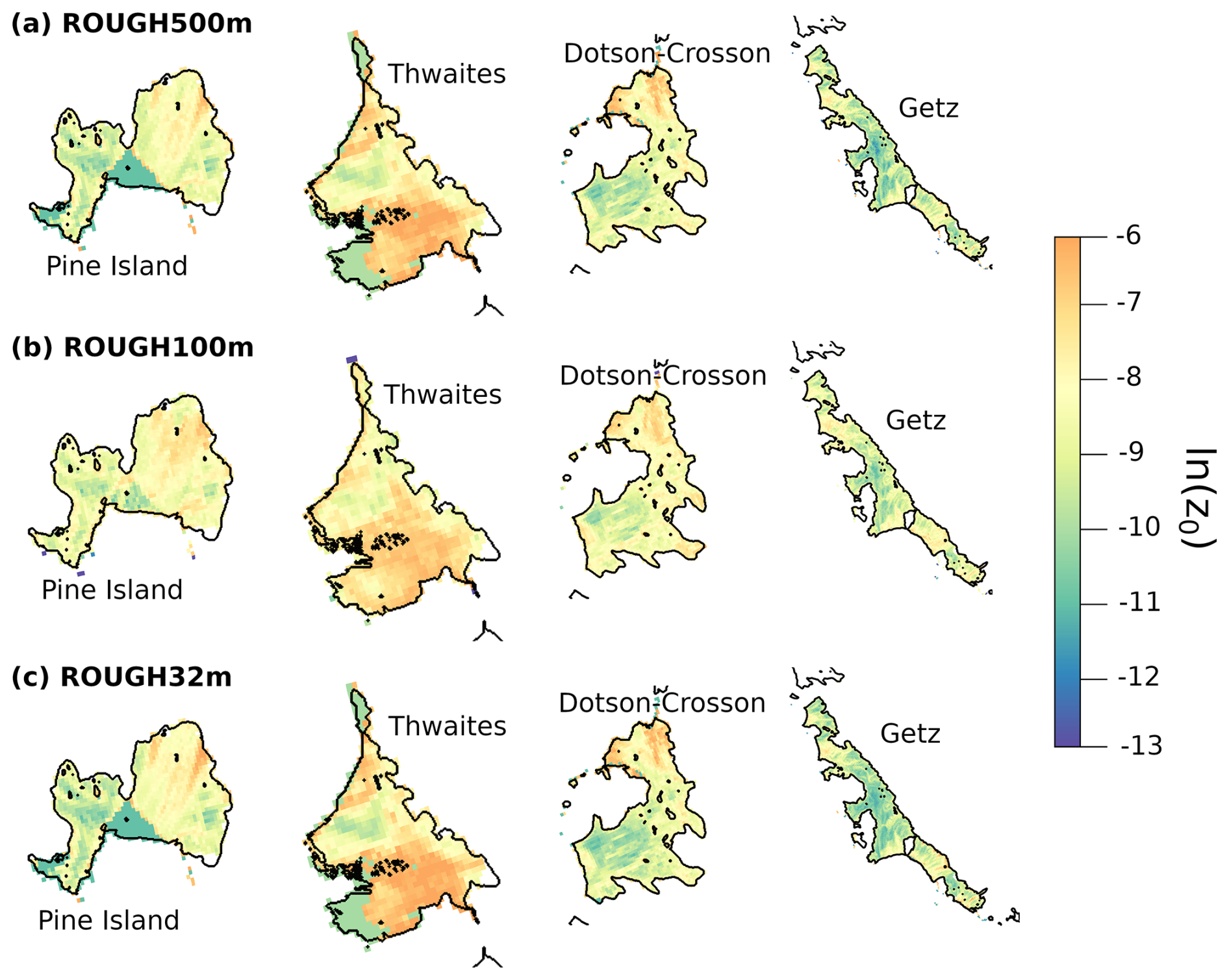
Figure 8 Hydrographic roughness length, z₀=αR, used in (a) ROUGH500m and R from Morlighem et al. (2019), (b) ROUGH100m and R from Howat et al. (2022), (c) ROUGH32m and R from Howat et al. (2022).

To compare results, we choose to look at the melt rate (in m yr⁻¹) and the total melt rate (in Gt yr⁻¹) averaged over the year 2013. We do not conduct a thorough evaluation of the simulations as this was already done in Jourdain et al. (2022).

We first compare REF and LOG experiments to show the effects of the new parameterisation. Second, we evaluate the vertical dependency of both parameterisations by comparing simulations with 121 vertical layers (REF and LOG) and 75 vertical layers (REF.L75 and LOG.L75), which is the standard number of layers in global Earth System Models using NEMO as an ocean model. Third, we compare them with simulations with constant C_d computed in the first wet cell for 75 and 121 vertical layers to evaluate the impact of the law of the wall. Fourth, we estimate the impacts of having a spatially variable z₀ compared to LOG experiment. We use the “topographic roughness”, R, calculated from the three different sub-shelf topography resolution datasets described in Sect. 2.1.3 and shown in Fig. 8: 500 m in ROUGH500m (Morlighem et al., 2019), 100 m in ROUGH100m (Howat et al., 2022), and 32 m in ROUGH32m (Howat et al., 2022). Boxplots of ln (z₀) for each ice shelf are shown in Fig. 9a with the horizontal line being the value for ln (z₀) in the LOG. Figure 9b shows C_d as a function of ln (z₀) for different half thickness z. All experiments are summarized in Table 2. Finally, we estimate the impacts of an increase of ice shelf roughness, as a potential future damage evolution, by increasing the roughness length, z₀. We choose to have a mean roughness, R, equal to the maximum roughness of the ROUGH experiment in LOGx5.

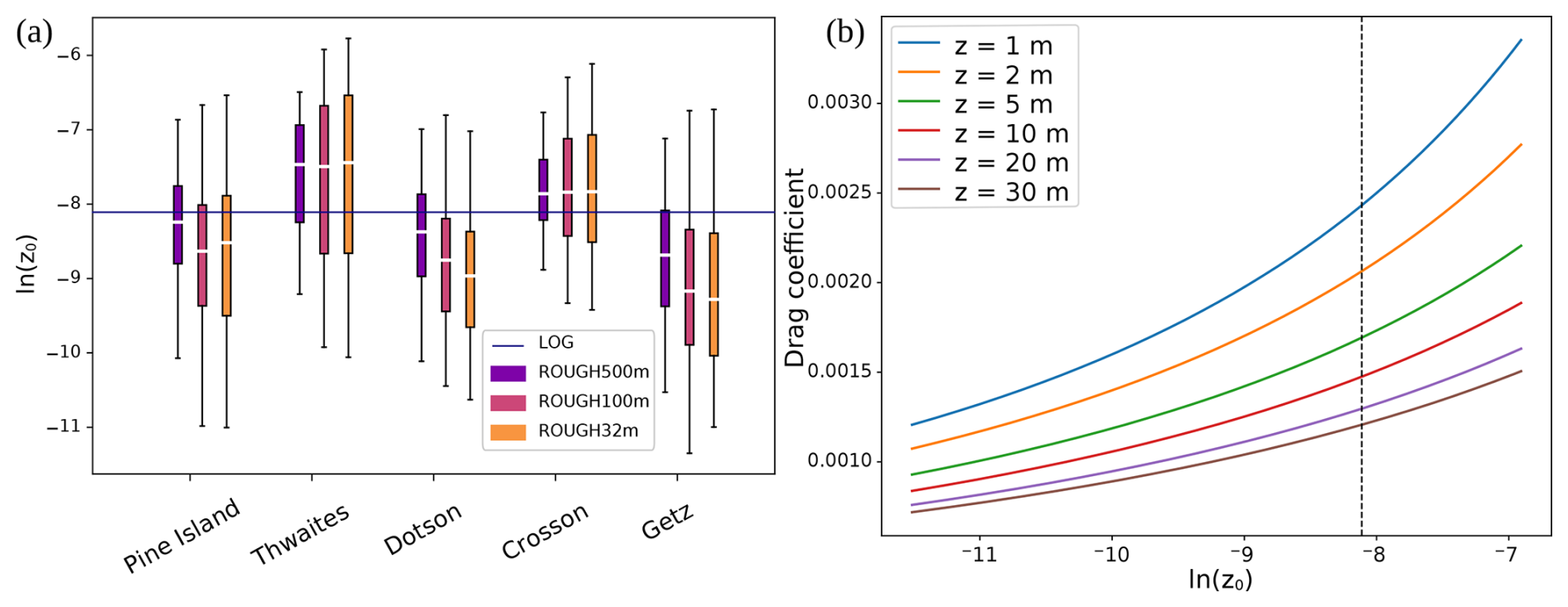
Figure 9 (a) Boxplot of ln (z₀) for ROUGH500m, ROUGH100m and ROUGH32m experiment and each ice shelf where the regional z₀ average is equal to the one used in LOG experiment ($\mathrm{3}\times {\mathrm{10}}^{-\mathrm{4}}$). The white line in each box is the median and the boxes are between the 25th and the 75th percentile. Whiskers ends show the 2nd and 98th percentile. The blue horizontal line represents the LOG hydrographic roughness length. (b) Drag coefficient as a function of ln (z₀) for different first wet cell half thickness z. Vertical dashed line shows $z_{\mathrm{0}}=\mathrm{3}\times {\mathrm{10}}^{-\mathrm{4}}$ m which is the value used in LOG experiment.

Morlighem et al. (2019)Howat et al. (2022)Howat et al. (2022)

Table 2 Experiments descriptions of different drag parameterisations.

3 Results and discussion

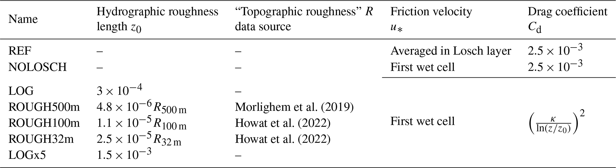
Table 3 summarizes the relative differences in total melt rates between different experiments for each ice shelf and for the ASE region. Comparisons between experiments are described below.

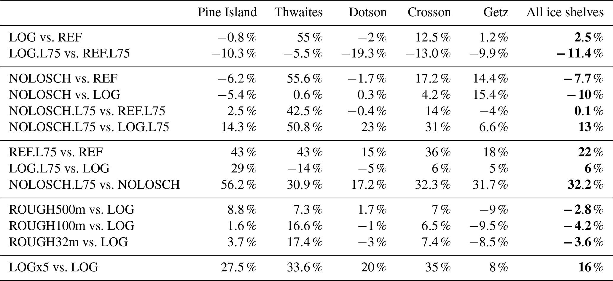
Table 3 Total melt rates relative differences for each ice shelf. Melt rates for all ice shelves are in bold.

3.1 Constant hydrographic roughness length vs. Constant drag coefficient (LOG vs. REF)

Figure 11a shows the basal melt rates produced in the REF experiment. Higher melt rates are generally present in regions below 500 m depth, which corresponds to where the modified Circumpolar Deep Water (mCDW) is entering the cavities in the ASE and where the freezing point temperature is lower (compare Figs. 3 and 11a). In shallower regions, melt rates are lower except at places where the buoyant melt-enriched water is following the slope of the ice shelf, generally concentrated in meltwater channels.

We chose a z₀ so that the total melt rates of the ASE region in LOG and REF are similar (see Fig. 10 and Table 3) with an overall regionally averaged relative difference of 2.5 %. Ice shelves in the LOG experiment are generally experiencing more melt than in REF but the relative differences are variable from one ice shelf to the other. Total melt rates of Pine Island ice shelf from LOG and REF are very close (−0.8 % difference) but they differ greatly in the case of Thwaites ice shelf (55 % difference).

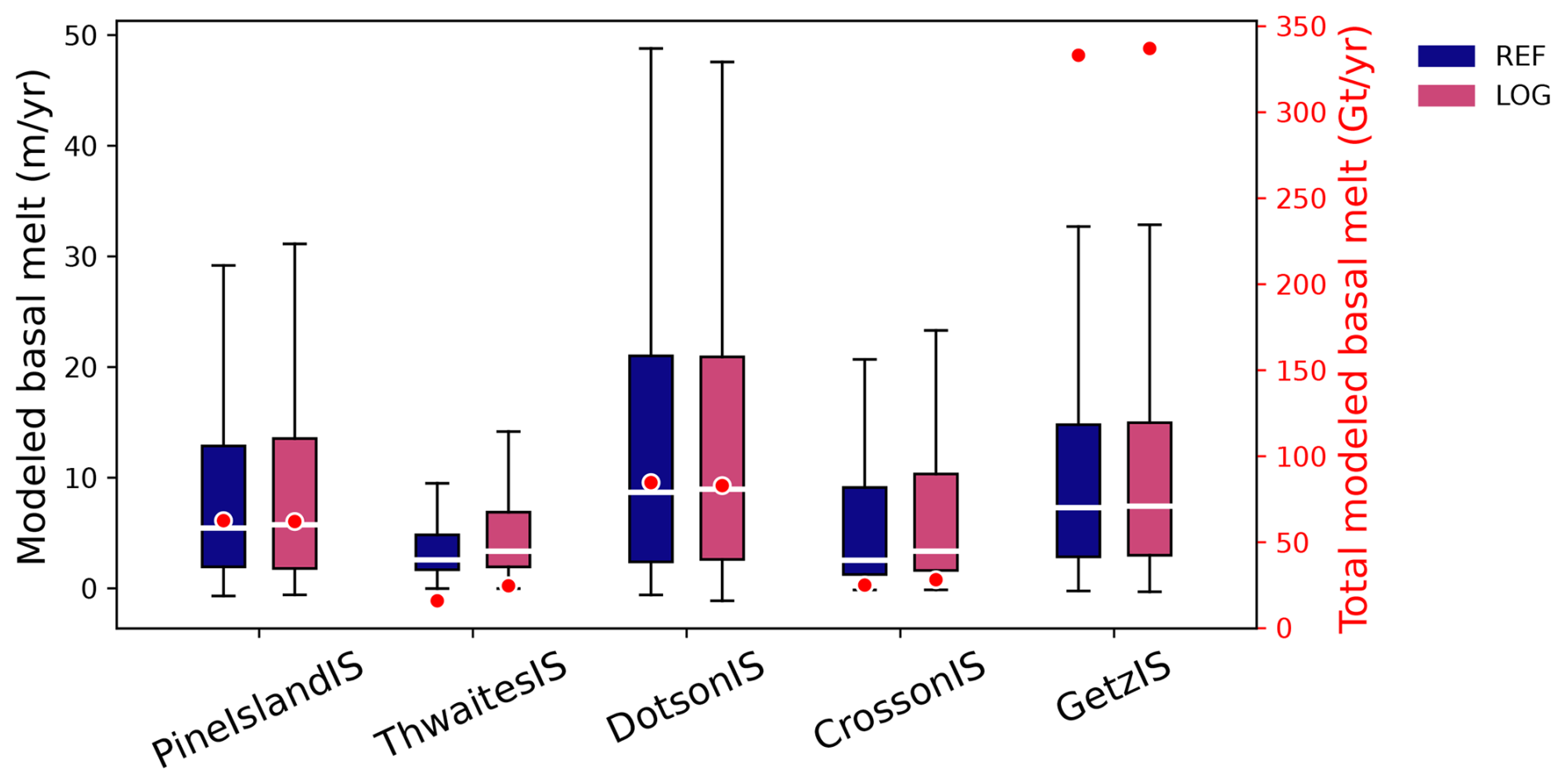
Figure 10 Boxplot of modeled basal melt (in m yr⁻¹) for REF (blue) and LOG (pink) on left y axis and total modeled basal melt (red points) for each ice shelf on right y axis. The white line in each box is the median and the boxes are between the 25th and the 75th percentile. Whiskers ends show the 2nd and 98th percentile.

The absolute difference between basal melt rates (see Fig. 11b), reveals spatially interesting features, which are not random as is the thickness of the first wet cell (Fig. 4). Even though total melt rates are similar, the difference can be non negligibly positive or negative (∓ 15–20 m yr⁻¹ difference at places of high melt). This probably means that spatial pattern differences tend to be compensated, with the exception of Thwaites ice shelf where most of the extra freshwater is produced close to the grounding line and particularly in the western sector.

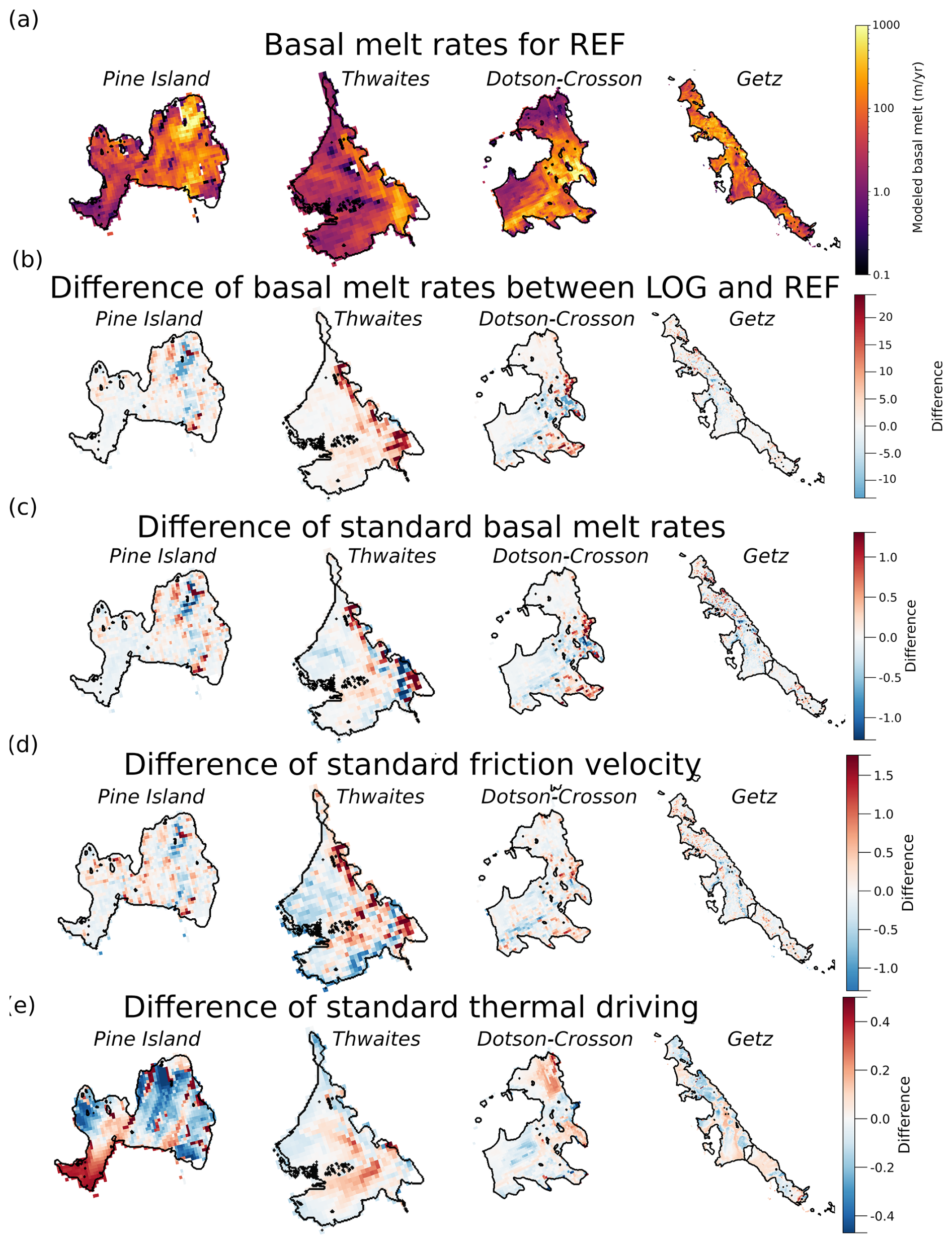
Figure 11 (a) Basal melt beneath each ice shelf for REF (in m yr⁻¹). We use a logarithmic color scale. (b) Basal melt absolute difference between LOG and REF (in m yr⁻¹) for each ice shelf. (c) Standardized basal melt absolute difference between LOG and REF for each ice shelf. (d) Standardized friction velocity (i.e., the deviation from the mean divided by the SD) absolute difference between LOG and REF for each ice shelf. (e) Standardized thermal driving absolute difference between LOG and REF for each ice shelf.

In order to compare the spatial differences between LOG and REF relative to the mean, we standardize the data (i.e., we calculate the deviation from the ice shelf mean and divide it by the SD so that data is in SD units). It is particularly interesting for Thwaites ice shelf since the mean difference of basal melt rates is so high. With standardized melt rates, it is possible to also see that there is a spatial pattern in melt rates differences for Thwaites ice shelf (Fig. 11c) but the areas with lower melt rates do not compensate for the much higher rates near some parts of the grounding line. Remarkably, melt rates in Thwaites and Dotson basal channels are lower in LOG than in REF.

In the three equation model (Eq. A1), melt rates depend on the friction velocity (through the drag coefficient, C_d, the mean horizontal current speed, U_M, the thermal driving, $T_{*}=T_{\mathrm{B}}-T_{\mathrm{M}}$ and the salinity, S_M). In Fig. 11d and e, we can see the differences of the standardized value of the two most important contributors, the friction velocity and the thermal driving (salinity difference is negligible). The spatial pattern of melt rate differences and their magnitude is very similar to the spatial pattern of friction velocity. This was expected as the difference between these two experiments is in the treatment of the friction velocity. Nevertheless, thermal driving differences are not negligible.

Knowing that friction velocity is the main difference contributor, it is interesting to compare both treatments of friction velocity (from the logarithmic and the Losch layer approach) within one single experiment. Figure 12a shows the friction velocity differences between LOG and REF and Fig. 12b shows the difference of friction velocity treatments within the LOG experiment. Spatial patterns are once again similar. To go further, we can look at the difference of mean horizontal current speed, U_M, as shown in Fig. 12c. At a first order, the differences of friction velocity between LOG and REF (Fig. 12a) are similar to the differences between current speed in the first wet cell, u_1wc, and averaged in the Losch layer, u_tbl although it does not apply to the Eastern sector of Thwaites ice shelf close to the grounding line. Melt rates are therefore directly related to the U_M treatment change in the three equation parameterisation.

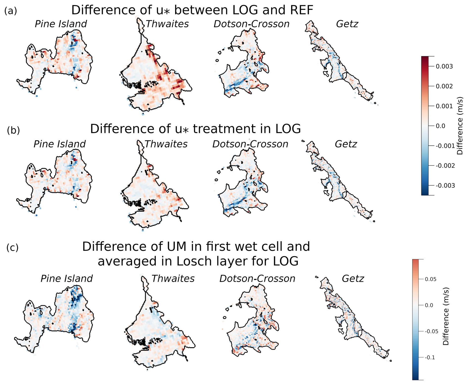
Figure 12 (a) Difference between friction velocities in LOG and REF. (b) Difference between friction velocity treatments (logarithmic approach and Losch layer approach) in LOG experiment. (c) Absolute difference between the mean horizontal current speed, U_M, in the first wet cell, u_1wc, and averaged in the Losch layer, u_tbl (in m yr⁻¹) for the LOG experiment for each ice shelf. In blue u_1wc<u_tbl and in red u_1wc>u_tbl.

It is interesting to note that the current speed in the first wet cell can be higher than the average in the Losch layer. This is due to the fact that, in the current version of NEMO, using the Losch layer approach, the mean horizontal current speed, used in the calculation of the friction velocity, is the magnitude of the component averages and not the average of the magnitudes:

$$\begin{array}{}\text{(4)}& U_{\mathrm{M}}^{\mathrm{2}}=u_{u,\text{tbl}}^{\mathrm{2}}+u_{v,\text{tbl}}^{\mathrm{2}}\end{array}$$

meaning that a change of speed direction in the column could induce a lower U_M in the Losch layer than in the first wet cell. Also, if the vertical resolution is coarse the friction velocity might be over- or underestimated depending on the actual velocity profile. Finally, if the first wet cell is thicker than the default Losch layer, this effect can be even stronger and the use of a constant C_d, representative of a constant Losch layer depth, is misleading.

3.2 Vertical resolution of 75 levels vs. 121 levels (REF.L75 vs. REF and LOG.L75 vs. LOG)

To assess the vertical resolution dependence of the drag coefficient treatement in ice shelf melt, we compare “global Earth System Model type” vertical resolution (75 levels) to an “ice shelf model type” vertical resolution (121 levels) as described in Sect. 2.1.2. Particularly, we look at the melt differences between the two vertical resolutions for experiments with the Losch layer approach (REF.L75 vs. REF) and with the logarithmic approach (LOG.L75 vs. LOG).

In Table 3, we can see very strikingly that the Losch layer approach is more dependent on the vertical resolution, with 22 % melt rate difference for the ASE region, than the logarithmic approach, with 6 % melt rate difference. Each ice shelf has a different dependency with Pine Island having the most differences between the two resolutions (43 % for the REF and 29 % for the LOG). Thwaites melt estimated in REF.L75 is much greater than in REF (43 %) and somewhat lower in LOG.L75 than in LOG (−14 %). Dotson, Crosson and Getz ice shelves show a diverse but relatively high dependency to vertical resolution in REF (15 %, 36 % and 18 % respectively) but this dependency is around 5 % in LOG. The spatial differences are presented in Fig. 13 showing most differences close to the grounding line, particularly at Pine Island ice shelf and on the eastern part of Thwaites ice shelf.

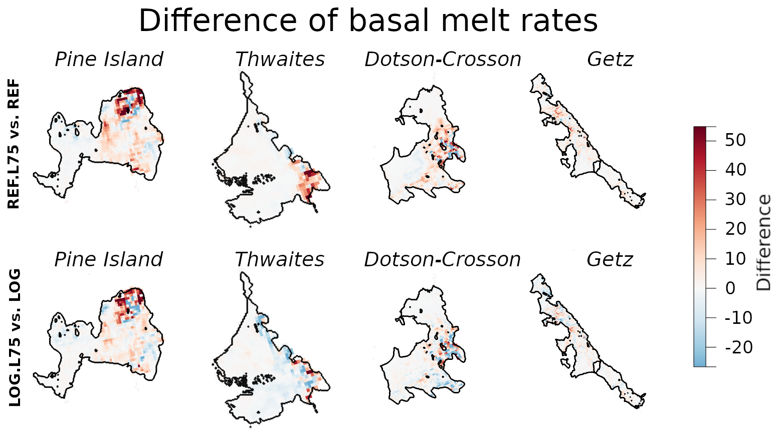
Figure 13 Absolute differences between configurations with 75 vertical levels and 121 vertical levels for each ice shelf. The upper panel compares configurations with constant drag coefficients (REF.L75 vs. REF) and the lower panel compares configurations with constant hydrographic roughness length (LOG.L75 vs. LOG).

With 121 levels, the Losch layer contains at least two cells (Fig. 6a) with the sum of their thickness close to 30 m (Fig. 6b). On the contrary, with 75 levels, the Losch layer may only contain one or two cells, and while the first wet cell is rescaled and might be smaller than the Losch layer thickness, the second cell thickness is already greater than 30 m below 300 m depth and increases exponentially to the grounding line. Moreover, if the first wet cell thickness is equal to or thicker than the Losch layer thickness, we are back to the same problem as described by Gwyther et al. (2020). Essentially, the cell thickness is variable but the drag coefficient is constant. If the first wet cell thickness is thinner than the Losch layer, with a coarse resolution, we use the weighted velocity of the next cell below (as explained in Appendix B1), which could have a thickness much thicker than the Losch layer. In this context, depending on the velocity profile, the Losch layer speed could be under- or overestimated.

3.3 Law of the wall versus constant drag in the first wet cell

To better evaluate if the law of the wall used in the LOG parameterisation is important or if it is as good as using a constant drag coefficient in the first wet cell, we compare NOLOSCH, LOG and REF experiments for 75 and 121 layers. With 121 layers, melt rates for NOLOSCH.L121 are closer to LOG.L121 than to REF.L121 for Thwaites, Crosson, Pine Island and Dotson ice shelves and slightly above for Getz ice shelf. On the contrary, with 75 levels, the total melt difference for all ice shelves is 0.1 % between NOLOSCH.L75 and REF.L75 % and 13 % between NOLOSCH.L75 and LOG.L75 with clear discrepency for individual ice shelves. So in summary, NOLOSCH is slightly closer to LOG than to REF with 121 layers and much closer to REF than to LOG with 75 layers.

Moreover, and most importantly, the difference between NOLOSCH.L75 and NOLOCH.L121 (32.2 % for all ice shelves) is much higher than between LOG.L75 and LOG.L121 (6 %) and even REF.L75 and REF.L121 (22 %). This means that it is absolutely not equivalent to have a constant or variable drag coefficient in the first wet cell.

To understand better why melt rates from NOLOSCH are closer to LOG when there is 121 levels and to REF with 75 levels, we plot the histogram of drag coefficient (Fig. 7b) and the histogram of cell half thickness (Fig. 7c) for all ice shelves for 121 and 75 levels. For 121 levels, cell half thickness is always smaller than 10 m and the drag coefficient is between $\mathrm{1.4}\times {\mathrm{10}}^{-\mathrm{3}}$ and $\mathrm{2.6}\times {\mathrm{10}}^{-\mathrm{3}}$ while for 75 levels the cell half thickness can be up to 30 m and the drag coefficient down to $\mathrm{1.0}\times {\mathrm{10}}^{-\mathrm{3}}$. In other words, LOG.L121 drag coefficient is closer to $\mathrm{2.5}\times {\mathrm{10}}^{-\mathrm{3}}$ than LOG.L75 and therefore NOLOSCH.L121 melt rates are closer to LOG.L121 although the difference is not that strong for all ice shelves. On the contrary, LOG.L75 drag coefficient can be much lower than $\mathrm{2.5}\times {\mathrm{10}}^{-\mathrm{3}}$ while the first wet cell thickness is closer to the Losch layer thickness used in REF.L75. For that reason, NOLOSCH.L75 is closer to REF.L75. It would have been interesting to run a NOLOSCH experiment with a drag coefficient close to the average of the LOG experiment. Nonetheless it shows that a variable drag coefficient, depending on the cell thickness, gives finer results and can be used the same way in any configuration, regardless the vertical resolution. In a nutshell, because of the high range of cell thickness (from 1 to 20 m for 121 levels and up to 60 m for 75 levels), having a constant or variable drag coefficient on the first wet cell is not equivalent.

3.4 Constant z₀ (LOG) versus spatially variable z₀ (ROUGH)

Here, we use the “topographic roughness”, R, as a proxy to a variable hydrographic roughness length, z₀ with different initial topography resolutions (ROUGH500m, ROUGH100m and ROUGH32m) as presented in Table 2. It is important to note that, even if the mean hydrographic roughness lengths for all considered ice shelves for the ROUGH experiments are equal to the constant hydrographic roughness length used in the LOG experiment, it does not imply that the mean hydrographic roughness length for an individual ice shelf is the same between the ROUGH experiments as can be seen in Fig. 9a. Here, we are therefore mostly interested in melt rates differences relative to each ice shelf's mean melt rates so that the standardized variable is preferred.

In Table 3, we see the relative difference of total melt rates between the ROUGH experiments and LOG. The total melt rates of the region are lower by 3 %–4 % for the ROUGH experiments compared to the LOG experiment. Dotson, Crosson and Getz ice shelves have similar total melt rates across roughness resolution (1 %–3 %, 6 %–7 % and 8 %–9 % difference respectively) while Pine Island ice shelf (1 %–9 % difference) experiences more melt in the coarsest resolution (500 m) and Thwaites ice shelf (7 %–17 % difference) on the two finer resolutions (100 and 32 m).

Figure 14a shows the difference of standard basal melt rates between the three ROUGH experiments and the LOG. From the comparison between the hydrographic roughness length, z₀=αR in Fig. 8 (plotted as ln (z₀)) and the melt rates differences in Fig. 14a, at a first glance, we get higher melt rates in places of higher z₀. ROUGH32m shows sharper contrast in places of finer topographic patterns (see Fig. 3), particularly in channels or at damaged zones. In Fig. 8, we can see for instance that at 500 m resolution, the shear margin of Pine Island ice shelf is not as well represented as in 100 or 32 m resolution. The hydrographic roughness length of the western part of Thwaites and the eastern part of Crosson are more pronounced for higher resolutions.

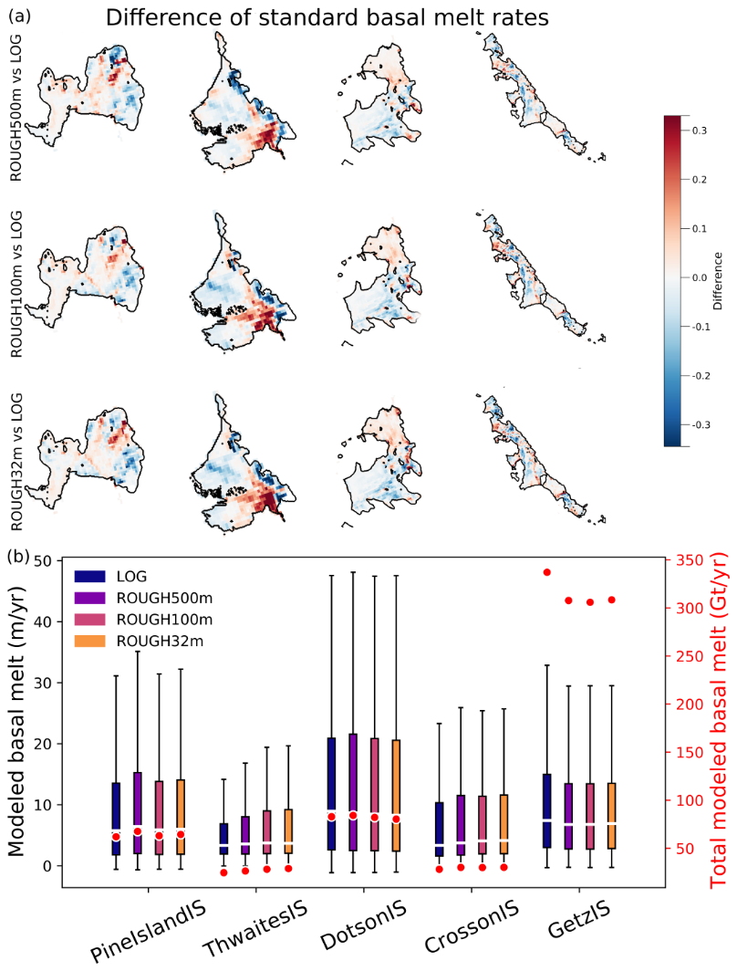
Figure 14 (a) Difference of standard basal melt rates (in m yr⁻¹) between different ROUGH experiments and LOG. (b) Boxplot of modeled basal melt (in m yr⁻¹) for LOG (blue) and all different ROUGH experiments on left y axis and total modeled basal melt (red points) for each ice shelf on right y axis.

3.5 Increased damage (LOGx5 vs. LOG)

As the ocean melts the ice below ice shelves and the ice is flowing, the geometry and the subgrid scale topography of the ice will change in time, due to ice shelf thinning and increased damage, and might have a very different pattern in the future. If we assume that drag is a function of “topographic roughness”, as we do in this study, it is worth looking at the sensitivity of melting to an increase of “topographic roughness” on melt. Here we imagine that the geometry is unchanged but the mean hydrographic roughness length of the region has increased to the maximum value of today from ROUGH500m (18 % total change of ln (z₀)). In this case, the total melt rates of the region would increase by 16 % (27 % for Pine Island ice shelf, 34 % for Thwaites ice shelf, 20 % for Dotson ice shelf, 35 % for Crosson ice shelf and 8 % for Getz ice shelf). The increase in melt rates averaged for the region is almost proportional to the amount of change in the logarithmic roughness length (16 % and 18 % respectively). However, when looking at each ice shelf independently, the same increase of z₀ is producing different effects on melt rates. In Fig. 9b, the drag coefficient is plotted against ln (z₀) for different cell half thickness z. This is only giving a partial picture of what the melt rates would look like because of its dependency on velocity, temperature, salinity. Nonetheless, one may see it as a coarse way to speculate on the roughness sensitivity.

3.6 Limits of the study

Six limits can be identified in this study and should be considered when using this drag parameterisation or to go further in the direction of implementing a variable hydrographic roughness length in the melt equation.

The first one is inherent to the parameterisation of the melt (the three-equation parameterisation) as it has been established for well-mixed turbulence regimes and is known to poorly perform under certain conditions by overestimating melt rates (Davis and Nicholls, 2019; Vreugdenhil and Taylor, 2019; Davis et al., 2023; Rosevear et al., 2024) when stratification is strong (Kimura, 2017), or when fluid velocity is weak (McConnochie and Kerr, 2017).

In the framework of shear melting, the second caveat comes from the use of a theoretical law (the law of the wall) that is only valid in the logarithmic layer and in certain conditions (surfaces with no slope, neutrally-stratified flow) (Raupach et al., 1991). This is designed for constant-stress boundary layers adjacent to an interface that is hydraulically smooth. It can cope with a variable roughness length, as used here, but only as long as that topographic roughness is not larger than the viscous boundary layer depth, such that it would start to disturb the boundary layer with lee eddies, etc.

Vertical mixing in the model is parameterized using a Turbulent Kinetic Energy (TKE) closure scheme, which determines the vertical eddy viscosity and diffusivity coefficients, a lower-bound cut-off is applied to ensure numerical stability and physical consistency, through a prognostic equation for the specific TKE. Its time evolution is governed by a balance between shear-induced production, buoyant destruction via stratification, vertical diffusion, and a Kolmogorov-type dissipation (Madec et al., 2022). At high resolution, it is therefore unlikely to have a similar velocity profile from one grid resolution to another.The third caveat is in the fact that NEMO, and our configuration does not resolve the log-layer. The top cell thickness is usually more than 1 m, and even with a thin top partial cell, the thickness of the cells below is generally ∼20 m so that there is no way to correctly resolve the log layer even if the viscosity parameterisation was suitable. Therefore, the log formulation is applied to all model cells beneath ice shelves, it is imposed exactly because NEMO does not produce such vertical log profiles.

Fourth, Losch (2008) and other studies only use averaged temperature and salinity in the Losch layer while we also use averaged velocities in the standard experiments. It is therefore possible that the added value of the new parameterisation is lower in models that do not average velocities in the Losch layer, although a part of the added value is not related to the Losch layer itself.

Fifth, the definition of the “topographic roughness” is arbitrary and other equations could be considered such as:

• a roughness estimation based on the obstacle height, the silhouette area and the specific area (Lettau, 1969).

• an effective roughness in heterogeneous terrain as developped for gentle slopes (Taylor, 1987) or steep slopes (Mason, 1991), using the subgrid slope. Hughes (2022) used this parameterisation to conceptualise ocean currents passing through an idealised mélange.

• the form and skin drags formulation as developped for sea ice melt (Lu et al., 2011; Tsamados et al., 2014).

• a function of the deformation energy developped for sea ice (Steiner et al., 1999; Steiner, 2001).

• any other roughness definition based on the topographic map or the observation transects (i.e. Watkins et al., 2021).

The subgrid roughness product depends not only on the roughness definition but also on the horizontal resolution of the ocean model. The coarser a grid is the smoother any topographical feature will be and it surely has an impact on the melt rates result. Moreover, the tuning parameter is not the constant drag coefficient itself but this $\mathit{\alpha }=z_{\mathrm{0}}/\overline{R}$, which has no physical basis and depends on the topographic map resolution.

Finally, the “topographic roughness” in this study is static in time and based on an observed topographic map. In reality, the geometry and the “topographic roughness” changes in time, shaped by the melt, the flow and the calving rate. A coupled approach is therefore necessary. An interesting line of research for a coupled ocean-ice sheet model would be to use a damage variable based on shear stress although correlation between damage and roughness is still to be proven (Watkins et al., 2024).

4 Conclusions

In this study, we present a new way to parameterise the friction velocity in the shear-controlled three-equation melt parameterisation in the ice shelf module in ocean model NEMO. Instead of using a Losch layer approach with a tuned drag coefficient constant in space and time and an horizontal current speed averaged in the Losch layer, we use a logarithmic approach, with a tuned hydrographic roughness length injected in the law of the wall and the first wet cell horizontal current speed. To go further, we investigate the dependency of basal melting to a spatially varying hydrographic roughness length, assuming that the hydrographic roughness length is proportional to the “topographic roughness” through a tuned coefficient. The aim is to represent the effect of subgrid scale topography, i.e., ice damage (multiple basal crevasses) and basal channels where melt rates are observed to be more important than in flat areas.

Our six main findings are:

• the Losch layer approach with a constant drag coefficient is highly dependent on the vertical resolution and inaccurate in coarse vertical resolution where the effective Losch layer thickness is thicker than the Losch layer thickness parameter or when the horizontal velocity is changing sign within the layer,

• for a given vertical resolution, the difference between using the top cell and the Losch layer is of comparable importance to using the law of the wall or a constant drag,

• the logarithmic approach is less dependent on the vertical resolution than the Losch layer approach (6 % versus 22 % difference) and provides similar total melt rates as the Losch layer approach,

• Removing the Losch layer makes the grid scaling worse (32 % versus 22 %) so the law of wall is necessary to get better scaling (6 %),

• the “topographic roughness” approach produces more melt in highly crevassed zones or in melt channels but can be sensitive to the resolution of the subgrid-scale topography data used to estimate the modelled roughness,

• an increase of hydrographic roughness length to the maximum present day value leads to increase melt rate.

These findings may have important consequences on future basal melt given the observed and foreseen increase of damage below ice shelves. This study has been performed in the Amundsen Sea Embayment region, where ice shelf cavities are particularly warm and where the current is vigourous. It would be worth looking at other types of ice shelves and see if the conclusions holds. In future climate scenarii, the ocean temperature increases and it would be interesting to quantify the effects on the melt rates using the new parameterisation.

As far as we know the effect of increasing damage on melt rates has not received a lot of attention so far, and there are feedbacks between melt rates and ocean velocity and temperature that may give unexpected melt sensitivity to roughness. It would therefore be interesting to explore further the effects of damage with a broader range of experiments.

This study shows the positive feedback of the hydrographic roughness length used in the melt parameterisation on ice shelf basal melt. It also shows the importance of better representing spatially variable ice–ocean drag for large-scale melt patterns, and it is an incentive to put more effort in the development of more realistic laws for turbulent transfer at the ocean-ice interface.

Appendix A: Three-equation or shear-controlled parameterisation

Melt rate, m, is solved with equations of heat conservation (Eq. A1), salt conservation (Eq. A2) together with the freezing point dependence at the ice–ocean interface (Eq. A3) such as

$$\begin{array}{}\text{(A1)}& {\displaystyle }-{\mathit{\rho }}_{\text{fw}}m{L}_{\mathrm{f}}={\mathit{\rho }}_{\text{sw}}{c}_{\text{sw}}{\mathit{\gamma }}_{\mathrm{T}}(T_{\mathrm{B}}-T_{\mathrm{M}})+{\mathit{\rho }}_{\text{fw}}{c}_{\mathrm{i}}{\mathit{\alpha }}_{\mathrm{i}}^{\mathrm{T}}{\displaystyle \frac{\partial T_i}{\partial z}}\text{(A2)}& {\displaystyle }-{\mathit{\rho }}_{\text{fw}}m{S}_{\mathrm{B}}={\mathit{\rho }}_{\text{sw}}{\mathit{\gamma }}_{\mathrm{S}}(S_{\mathrm{B}}-S_{\mathrm{M}})\text{(A3)}& {\displaystyle }{T}_{\mathrm{B}}={\mathit{\lambda }}_{\mathrm{1}}{S}_{\mathrm{B}}+{\mathit{\lambda }}_{\mathrm{2}}+{\mathit{\lambda }}_{\mathrm{3}}{p}_{\mathrm{B}}\end{array}$$

with ρ_fw, the fresh water density, c_sw, the sea water heat capacity, c_i, the ice heat capacity, ${\mathit{\alpha }}_{\mathrm{i}}^{\mathrm{T}}$, the ice thermal diffusity, L_f, the latent heat of fusion, λ_i, liquidus coefficients and p_B, the pressure (Jenkins et al., 2010).

Temperature and salinity are noted T_B and S_B respectively at the ice base while they are noted T_M and S_M at a distance from the ice, which can be different depending on the model one uses. Heat and salt from the ocean are mixed at the interface with the ice and these turbulent processes are described by ${\mathit{\gamma }}_{\text{T/S}}={\mathrm{\Gamma }}_{\text{T/S}}{u}_{*}$, the turbulent exchange velocities. Turbulent transfer coefficients for heat and salt, Γ_T/S are derived from sea ice observations (McPhee et al., 1987) as a function of buoyancy flux and later applied to ice shelves Holland and Jenkins (1999). Jenkins et al. (2010) showed that using observationally derived constants for Γ_T/S fits the data equally well for Ronne-Filchner Ice Shelf and many ocean models use constant Γ_T/S values.

Appendix B: Friction velocity treatment below ice shelves

In NEMO, the friction velocity, u_*, used in ice shelf thermodynamic and ocean dynamics equations follows a quadratic parameterisation (Eq. 2). The drag coefficient, C_d, can be constant or z-dependent and the cell(s) where the mean horizontal current speed, U_M, is sampled either in the Losch layer (REF experiment), or in the first wet cell as described in Sect. 2.3. Here we present more details on how the friction velocity is computed for the thermodynamic equation in NEMO where we use the Arakawa C-type grid and z^* coordinate system with partial steps on free boundaries as described in Sect. 2.1.2. The cell thickness follows a double hyperbolic tangent function and depends on the depth (see Fig. 5). The representation of the first wet cell (depending on the ice shelf boundary position) and the Losch layer are shown in the scheme of Fig. 2c.

B1 Constant drag coefficient: REF experiment

For the REF experiment, the drag coefficient is constant everywhere and the friction velocity depends on the magnitude of the current speed components averaged over the Losch layer and at T-point where melt rates are calculated.

First, the horizontal ocean velocity components, u and v sampled at U-point $(i+\frac{\mathrm{1}}{\mathrm{2}},j)$ and V-point $(i,j+\frac{\mathrm{1}}{\mathrm{2}})$ respectively, are averaged over the Losch layer to produce u_L at U-point and v_L at V-point.

$$\begin{array}{}\text{(B1)}& \left\{\begin{array}{ll}{u}_{\mathrm{L}}^{i+\frac{\mathrm{1}}{\mathrm{2}},j}=\frac{\mathrm{1}}{h_{\mathrm{L}}}{\sum }_{k=k_{\mathrm{t}}^{i,j}}^{k_{\text{bL}}^{i,j}}{f}_{\mathrm{L}}^{i+\frac{\mathrm{1}}{\mathrm{2}},j,k}{u}^{i+\frac{\mathrm{1}}{\mathrm{2}},j,k}{e}_{\mathrm{3}u}^{i+\frac{\mathrm{1}}{\mathrm{2}},j,k}& \\ & \mathrm{\text{at U-point}}(i+\frac{\mathrm{1}}{\mathrm{2}},j,k^{i,j})\\ v_{\mathrm{L}}^{i,j+\frac{\mathrm{1}}{\mathrm{2}}}=\frac{\mathrm{1}}{h_{\mathrm{L}}}{\sum }_{k=k_{\mathrm{t}}^{i,j}}^{k_{\text{bL}}^{i,j}}{f}_{\mathrm{L}}^{i,j+\frac{\mathrm{1}}{\mathrm{2}},k}{v}^{i,j+\frac{\mathrm{1}}{\mathrm{2}},k}{e}_{\mathrm{3}v}^{i,j+\frac{\mathrm{1}}{\mathrm{2}},k}& \\ & \mathrm{\text{at V-point}}(i,j+\frac{\mathrm{1}}{\mathrm{2}},k^{i,j})\end{array}\right.\end{array}$$

with hL the Losch layer thickness (equals the cell thickness if greater than the default Losch layer thickness), k_t, the first wet cell vertical coordinate, k_bL, the bottom cell of the Losch layer vertical coordinate, e_3u and e_3v the cell thicknesses at U-point and V-point respectively and f_L the fraction of the cell included in the Losch layer.

Second, u_L and v_L are averaged at T-point to finally compute the magnitude U_M used in Eq. (2).

$$\begin{array}{}\text{(B2)}& \left\{\begin{array}{l}{u}_{\mathrm{L}}^{i,j}=\frac{\mathrm{1}}{\mathrm{2}}(u_{\mathrm{L}}^{i-\frac{\mathrm{1}}{\mathrm{2}},j}+u_{\mathrm{L}}i+\frac{\mathrm{1}}{\mathrm{2}},j)\\ v_{\mathrm{L}}^{i,j}=\frac{\mathrm{1}}{\mathrm{2}}(v_{\mathrm{L}}^{i,j-\frac{\mathrm{1}}{\mathrm{2}}}+v_{\mathrm{L}}^{i,j+\frac{\mathrm{1}}{\mathrm{2}}})\\ U_{\mathrm{M}}^{i,j}=\left(\right(u_{\mathrm{L}}^{i,j}{)}^{\mathrm{2}}+(v_{\mathrm{L}}^{i,j}{)}^{\mathrm{2}}{)}^{\frac{\mathrm{1}}{\mathrm{2}}}\end{array}\right.\mathrm{\text{at T-point}}(i,j,k_{\mathrm{t}}^{i,j})\end{array}$$

B2 Constant and variable hydrographic roughness length: LOG and ROUGH experiments

For the LOG and ROUGH experiments, we use the law of the wall (Eq. 1) and the friction velocity, u_*, quadratic parameterization (Eq. 2) to calculate the drag coefficient, C_d, dependent on the depth, z, and on the hydrographic roughness length, z₀ (see Eq. 3). To smooth the treatment of u_* below ice shelves, we linearly interpolate C_d in between two cells and calculate the resulting u_* at U-point $(i+\frac{\mathrm{1}}{\mathrm{2}},j,k_{\mathrm{t}}^{i,j})$ and V-point $(i,j+\frac{\mathrm{1}}{\mathrm{2}},k_{\mathrm{t}}^{i,j})$ respectively, such as:

$$\begin{array}{}\text{(B3)}& \begin{array}{rl}{\displaystyle }\left\{\begin{array}{l}{z}_{\mathrm{0}}^{i+\frac{\mathrm{1}}{\mathrm{2}},j}=\frac{\mathrm{1}}{\mathrm{2}}(z_{\mathrm{0}}^{i,j}+z_{\mathrm{0}}^{i+\mathrm{1},j})\\ C_{\mathrm{d}}^{i+\frac{\mathrm{1}}{\mathrm{2}},j}={\mathit{\kappa }}^{\mathrm{2}}{\left(\ln \frac{z^{i+\frac{\mathrm{1}}{\mathrm{2}},j,k_{\mathrm{t}}^{i,j}}}{z_{\mathrm{0}}^{i+\frac{\mathrm{1}}{\mathrm{2}},j}}\right)}^{-\mathrm{2}}\\ u_{*u}^{i+\frac{\mathrm{1}}{\mathrm{2}},j}=\sqrt{C_{\mathrm{d}}^{i+\frac{\mathrm{1}}{\mathrm{2}},j}}{u}^{i+\frac{\mathrm{1}}{\mathrm{2}},j,k_{\mathrm{t}}^{i,j}}\end{array}\right.& {\displaystyle }\mathrm{\text{at U-point}}(i+\frac{\mathrm{1}}{\mathrm{2}},j,k_{\mathrm{t}}^{i,j})\\ {\displaystyle }\left\{\begin{array}{l}{z}_{\mathrm{0}}^{i,j+\frac{\mathrm{1}}{\mathrm{2}}}=\frac{\mathrm{1}}{\mathrm{2}}(z_{\mathrm{0}}^{i,j}+z_{\mathrm{0}}^{i,j+\mathrm{1}})\\ C_{\mathrm{d}}^{i,j+\frac{\mathrm{1}}{\mathrm{2}}}={\mathit{\kappa }}^{\mathrm{2}}{\left(\ln \frac{z^{i,j+\frac{\mathrm{1}}{\mathrm{2}},k_{\mathrm{t}}^{i,j}}}{z_{\mathrm{0}}^{i,j+\frac{\mathrm{1}}{\mathrm{2}}}}\right)}^{-\mathrm{2}}\\ u_{*v}^{i,j+\frac{\mathrm{1}}{\mathrm{2}}}=\sqrt{C_{\mathrm{d}}^{i,j+\frac{\mathrm{1}}{\mathrm{2}}}}{v}^{i,j+\frac{\mathrm{1}}{\mathrm{2}},k_{\mathrm{t}}^{i,j}}\end{array}\right.& {\displaystyle }\mathrm{\text{at V-point}}(i,j+\frac{\mathrm{1}}{\mathrm{2}},k_{\mathrm{t}}^{i,j})\end{array}\end{array}$$

with (u,v) the velocity components at U- and V-points.

Then we calculate u_* at T-point $(i,j,k_{\mathrm{t}}^{i,j})$ such as

$$\begin{array}{}\text{(B4)}& \left\{\begin{array}{l}{u}_{*u}^{i,j}=\frac{\mathrm{1}}{\mathrm{2}}(u_{*u}^{i-\frac{\mathrm{1}}{\mathrm{2}},j}+u_{*u}^{i+\frac{\mathrm{1}}{\mathrm{2}},j})\\ u_{*v}^{i,j}=\frac{\mathrm{1}}{\mathrm{2}}(u_{*v}^{i,j-\frac{\mathrm{1}}{\mathrm{2}}}+u_{*v}^{i,j+\frac{\mathrm{1}}{\mathrm{2}}})\\ u_{*}^{i,j}=\left(\right(u_{*u}^{i,j}{)}^{\mathrm{2}}+(u_{*v}^{i,j}{)}^{\mathrm{2}}{)}^{\frac{\mathrm{1}}{\mathrm{2}}}\end{array}\right.\text{at T-point}(i,j,k_{\mathrm{t}}^{i,j})\end{array}$$