A mathematical model of microbially-induced convection in sea ice

Through its role as an interface between ocean and atmosphere, sea ice is important both physically and biologically. We propose here that the resident microbial community can influence the structure of sea ice, particularly near its ocean interface, by effectively lowering the local freezing point via an osmolytic mechanism. This lowered freezing point can enhance fluid flow, linking a bottom, convective ice layer with the underlying ocean, resulting in improved nutrient uptake and byproduct removal. A mathematical model based on a previously suggested abiotic one dimensional simplification of mushy ice fluid dynamics is used to illustrate, and supporting measurements of freezing point depression by lab grown sea ice-associated organisms are provided.

1 Introduction

Sea ice in the polar regions is a fundamental cryospheric habitat that serves as an important component of Earth's climate system by regulating heat exchange between the atmosphere and ocean and also by reflecting sunlight (Ledley, 1991, 1993; Eicken and Lemke, 2001; Boeke and Taylor, 2018). It also supports diverse microscopic assemblages, including bacteria, algae, and various invertebrates, all essential for maintaining ecological balance (Arrigo and Thomas, 2004; Thomas and Dieckmann, 2008; Arrigo, 2014). During sea ice formation and growth, the progressive development of brine-filled channels establishes distinct physicochemical microenvironments that facilitate the colonization of specialized microbial communities, which can propagate to impact large-scale systems. This can have macroscale implications: in the polar oceans, sea ice serves as a critical environment influencing ecology and biogeochemical cycles (Comeau et al., 2013; Arrigo, 2014; Swadling et al., 2023), functioning as a refuge for larger organisms like seals and penguins, while providing habitat for communities of prokaryotes and eukaryotes on ice surfaces and within brine channels (Garrison et al., 1986; Bluhm et al., 2017; Kohlbach et al., 2018). Indeed, it appears that the structure and activity of sea ice microbial communities are considerably more complex than once thought (Audh et al., 2023).

Sea ice microbial communities serve as vital food resources for copepods and krill (Bluhm et al., 2017; Kohlbach et al., 2018) and influence fundamental ecological and atmospheric processes, including dimethylsulfide emissions, carbon dioxide uptake, methane release, and halogen chemistry (Fadeev et al., 2021; Steiner et al., 2021), influencing global biogeochemical cycles (Lannuzel et al., 2020). Laboratory studies have demonstrated that microbial communities can modify their habitat chemically (Zhou et al., 2014) but also physically, through alteration of sea-ice microstructure by pore clogging and depression of brine freezing points (Krembs et al., 2011). As sea ice continues to thin and transition toward predominantly first-year ice, these communities are adapting by initiating colonization earlier in the season and accumulating greater biomass over shortened periods, possibly facilitated by enhanced light penetration, with their ecological importance increasing as sea ice loss continues due to their adaptability to seasonal fluctuations in the carbonate system (Torstensson et al., 2021). While these mechanisms are known, their precise dynamics and quantification at large scales remain poorly understood and are generally absent from large-scale modeling (Vancoppenolle et al., 2013). Given the rapid transformation of polar regions, exploring the potential for a reciprocal relationship between large-scale marine biogeochemical processes and their resident microbial communities seems timely. In that spirit, we propose here the possibility that sea ice microbes can not only adapt to changing sea ice conditions but also modify the ice itself to maintain nutrient supplies.

1.1 Sea Ice

Sea ice itself would seem to be a difficult habitat, and while clear differences in community composition have not always been observed between sea ice and the surrounding water (Garrison et al., 1986; Dawson et al., 2023), metabolomics show differences suggesting mechanisms to cope with the changes in temperature and salinity between these two environments (Dawson et al., 2023). We focus here on interaction between the ice and its microbial community (the structure of sea ice is notable for its length scale dependence through a variety of physical mechanisms) at small scales, centimeters and below, where individual ice crystals, fundamental to sea ice's formation, are typically on the millimeter size. This scale reveals sea ice as a composite material composed of two main components: solid ice and liquid brine. Because of the connection to transport properties, composite details influence to a significant extent macro-properties including, notably here, biological productivity.

Sea ice is formed during colder seasons when air temperature can reach temperatures well below 0 °C. On the other hand, the temperature at the sea ice-ocean interface remains approximately −1.8 °C throughout the year and so, when the air temperatures drop sufficiently, ice formation can occur. As freezing occurs, impurities are excluded, leading to the formation of relatively high salinity brine inclusions in almost pure-water ice. Inclusion sizes become larger as the warmer (at least in colder seasons) ice-ocean interface is approached for thermodynamic reasons (discussed below in Sect. 1.2) (Kraitzman et al., 2022; Stewart et al., 2024). Near this interface, in a layer in which the ice temperature rises above a threshold temperature (Golden et al., 1998), brine inclusions interconnect to the point of forming a permeable material through which fluid can, in principle, flow and thus bring fresh seawater and accompanying nutrients (and microbes) (Tedesco et al., 2010).

The presence of an interconnected network does not by itself result in fluid flow though; there is also a need for a driving force capable of overcoming viscous drag. During periods of growth, flow within sea ice can be driven by density inversions in large part due to brine concentration (Worster, 1992, 1997, 2000; Feltham et al., 2006; Worster and Jones, 2015). That is, freezing of seawater results in relatively dense brine, through the concentration process described above, which can result in convective, Rayleigh-Taylor instabilities (Chandrasekhar, 1961) in which, roughly, the gravitational potential energy of a density inversion can be more easily released by convective versus diffusive transport. Convective flow requires interconnected channels, and the larger those channels, the easier convective transport becomes since viscous drag is sensitive to channel size. This draining process, however, relies on freezing of “new”, salty seawater by the advancing ice front though, and cannot maintain flow when freezing is not occurring. Hence the question arises of how microbial communities can sustain themselves within the ice, even in the permeable layer, when sufficient freezing is not occurring. We argue here that the microbes themselves can drive a convective flow.

1.2 Effective Salinity

Locally, sea ice temperature and brine inclusion concentration are often approximated as being close to thermodynamic equilibrium, since the local heat diffusion time scale is generally short compared to time scales of other relevant diffusive and advective transport processes of interest. That is, local brine inclusion salinity (we will use the term salinity in a specific sense related to effect of freezing temperature, discussed below) must be such that the local brine freezing point matches the local temperature, quantified through an empirical relation of the form ℒ(T)=S_brine, called a liquidus relation (see Appendix A3 for details). Here T (°C) is the local temperature and S_brine (ppt, parts per thousand) is the local brine salinity. Note also that total, or bulk, salinity S_bulk is conserved, locally, on short time scales, and that $S_{\mathrm{brine}}=S_{\mathrm{bulk}}/{\mathit{\varphi }}_{\mathrm{brine}}$ (where ϕ_brine is local brine volume fraction) so that the liquidus relation can be written in the form $\widehat{\mathcal{L}}(T,{\mathit{\varphi }}_{\mathrm{brine}})=S_{\mathrm{bulk}}$. As $\widehat{\mathcal{L}}$ is monotone increasing in ϕ_brine, then, given T and S_bulk, this relation can be inverted to solve for ϕ_brine.

Over longer time scales, though, local bulk salinity can change due to diffusive or advective transport, and, particularly in the presence of biological activity, due to chemical sources or sinks. We argue here that sea ice microorganisms can use such production to in fact manipulate ice permeability and, ultimately, help drive advective flow. Some sea ice micro-algae including diatoms, e.g., Rhizosolenia, Corethron, and haptophyta, e.g., Phaeocystis, and also heterotrophic species such as nanoflagellates and ciliates (Garrison et al., 1986; Caron and Gast, 2010; Kohlbach et al., 2018; Hop et al., 2020; Dawson et al., 2023) are known to produce metabolites in different distributions and concentrations in relation to change in environmental conditions including temperature and salinity (Dawson et al., 2020). For example, dimethylsulfoniopropionate (DMSP) and dimethylsulfide (DMS), which show antifreeze properties (Uhlig et al., 2019; Sheehan and Petrou, 2020), tend to increase inside the cells of micro-algae associated with sea ice compared to seawater: seawater at approximately 0.19 nmol metabolite C per total µmol C and sea ice at approximately 1.81 nmol metabolite C per total µmol C (Dawson et al., 2023). Other metabolites, such as proline and glycine betaine, are also produced in larger concentrations in ice conditions, and are known to increase freeze tolerance in other species (e.g., yeast for proline, Morita et al., 2003; Arabidopsis for glycine betaine, Xing and Rajashekar, 2001).

We explore here the possibility that at least some of these various substances may, among other things, effectively act as external antifreeze agents in the manner of osmolytes. To do so, we define an effective brine salinity as a combination S_brine+Y_salO_brine and replace S_brine in the liquidus relation by this effective brine salinity, see Appendix A for details. Here O_brine is a brine (microbially-origined) osmolyte concentration and Y_sal is a yield coefficient, converting osmolyte concentration to effective salinity. Osmolyte is measured in normalized units so that one unit of osmolyte has the same density effect as one unit of salt. The parameter Y_sal takes account of the relative salinity effect of osmolyte in these normalized units. For modeling purposes, we don't distinguish a particular choice of microbially produced osmolyte, or osmolytes, and so do not try to estimate a particular value for Y_sal. There did not seem to be a lot of sensitivity to choice of Y_sal in computations though, possibly because of two competing effects: increasing/decreasing Y_sal tends to increase/decrease brine volume fraction which increases/decreases permeability, but at the same time decreasing/increasing added density (from the extra osmolyte) which decreases/increases the density driven fluid driving potential.

2 Freezing Point Measurements: Materials and Methods

To test the impact of microalgae on ice formation temperature, we measured freezing points (e.g., Fujino et al., 1974) using the diatom Chaetoceros neogracilis (W-126 Chaetoceros, 97 % similarity to EU090012) from the Antarctic Protist Culture Collection, USA. This organism has been reported in sea ice and in seawater in the Arctic Ocean during pack ice melting (Gérikas Ribeiro et al., 2020) and often dominates phytoplankton community (Katsuki et al., 2009; Crawford et al., 2018). C. neogracilis is a solitary rectangular cell, measuring 4–10 µm in length (Scott and Marchant, 2005; Katsuki et al., 2009), and was isolated from the Ross Sea in 1999 on board the RVIB Nathaniel B Palmer. It has been maintained since in the laboratory in a non-axenic culture kept in 36 ppt Instant Ocean^® with $f/\mathrm{2}$ + Si media (Guillard and Ryther, 1962) in an incubator at 4 °C under illumination at 20 $\mathrm{\mu }\mathrm{mol}\mathrm{photons}{\mathrm{m}}^{-\mathrm{2}}{\mathrm{s}}^{-\mathrm{1}}$ 14:10 light : dark cycle. Cell abundance was approximately 7×10⁸ cell L⁻¹ during the experiment.

For the measurements, we used a simplified thermal calorimetric apparatus, see Fig. 1. A volume of 25 mL of liquid was placed in a 50 mL glass culture tube inside a 150 mL Nalgene plastic bottle, Fig. 1. To create a cold bath, the plastic bottle was placed in dry ice (−70 °C). Dry ice was used because its temperature is well below that of the freezing point of the culture liquid as well as to reduce the duration of the experiment and avoid any metabolic interference or death of the microalgae due to freezing, rendering more complicated the interpretation of the results. To ensure homogeneity of the cooling process, a magnetic stir bar was introduced into the 50 mL glass culture tube and the liquid was stirred at medium speed. Temperature was recorded each minute with a Traceable^® Excursion-Trac™ datalogging thermometer with stainless-steel probe, see Fig. 1. Using this apparatus, the freezing point of seawater (Instant Ocean) plus $f/\mathrm{2}$ media (nutrients for phytoplankton) and a diatom culture of Chaetoceros sp., suspended in seawater plus media, were assessed. Salinity of the culture medium itself (∼26.5 mg L⁻¹) was negligible compared to that of the seawater (∼11.1 g L⁻¹). To understand the impact of osmolytes produced by the diatoms on the freezing point, cultures were centrifuged at 7500 rpm for 10 min at 4 °C and the resulting liquid supernatant was used to measure the impact of osmolytes.

Each experiment was run for 30–40 min, until solidified ice was observed. To determine the freezing point, temperature was plotted over time. After a phase of cooling and then supercooling, the liquid changed state and ice nucleation began. The resulting ice formation released heat until the freezing point (plateau) was attained, at which an approximate equilibrium between crystal formation and melting occurs. The temperature was stable during this phase.

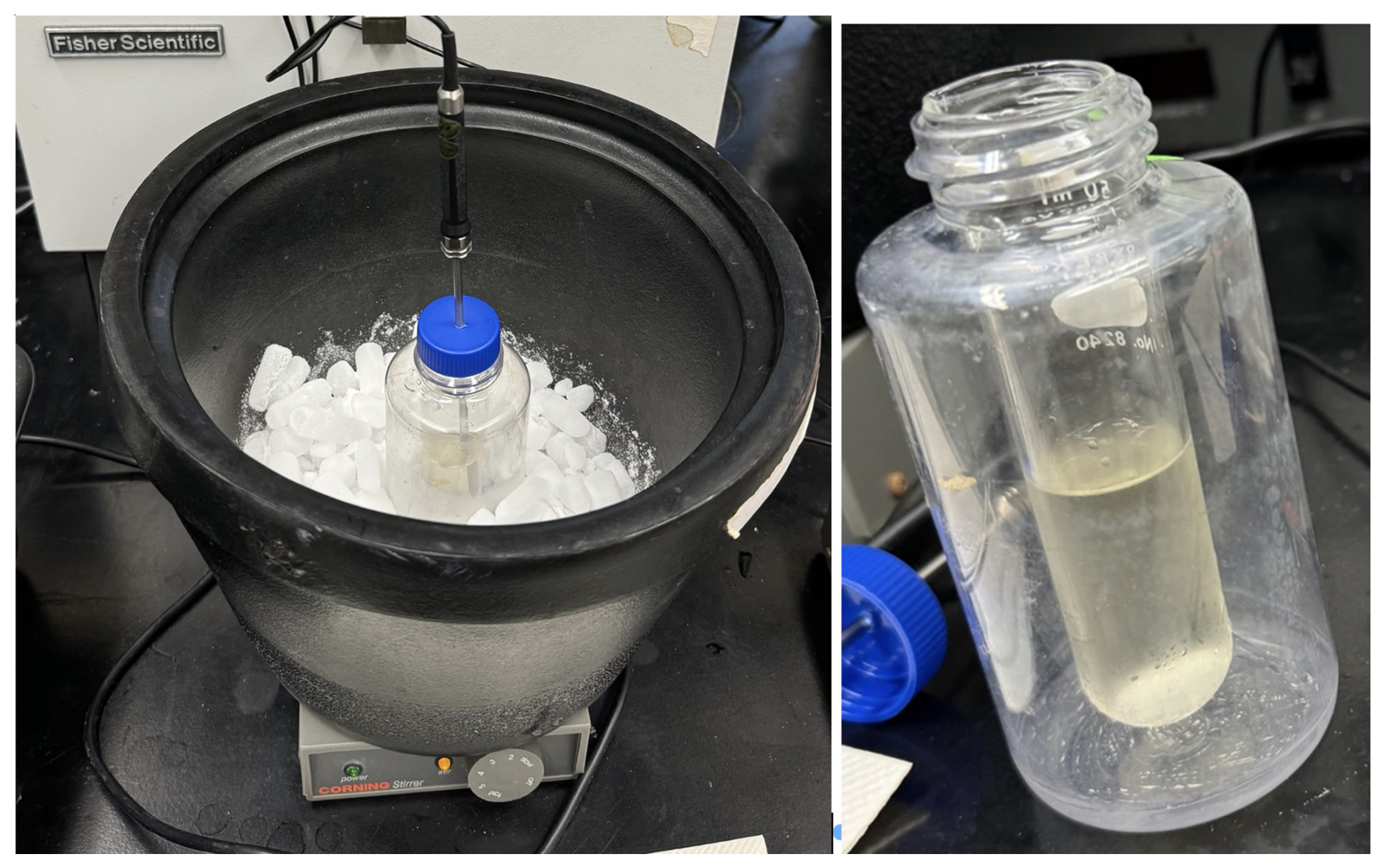
Figure 1 Freezing point measurement apparatus. Left: the thermal calorimetric apparatus constituted of an isolated bucket on a magnetic stir plate. The bucket contains dry ice in which a chamber is placed. Right: the chamber is composed of a 50 mL glass culture tube inside a polycarbonate 150 mL bottle.

3 Mathematical Model

Mathematical descriptions of phase behavior in abiotic sea ice have been based, often, on reaction-advection-diffusion equations for transport of bulk heat and salt, coupled to a liquidus relation (as described in Sect. 1.2) maintaining a local equilibrium between solid and brine phases (e.g., Worster, 1992, 1997). This equilibrium also sets local solid and brine phase volumes, which couple into a fluid dynamics description, typically modeled as a porous media (Darcy) flow. The entire system is driven by a temperature gradient vertically through the ice column, and can become quite complex. We employ a significant simplification of full sea ice dynamics, following Vancoppenolle et al. (2010); Griewank and Notz (2013); Turner et al. (2013); Griewank and Notz (2015), in which three dimensional mushy layer fluid dynamics are replaced by a one-dimensional (1D), parameterized reduction. That is, mushy ice velocity field u(x,t) is replaced by a 1D, non-negative upwards velocity $U(z,t)\widehat{\mathit{z}}$, driven by a modeled Rayleigh-Taylor instability mechanism. When the computed local Rayleigh number Ra(z,t) exceeds a critical Rayleigh number Ra_crit, material is removed and flushed into the ocean at rate proportional to Ra−Ra_crit, with U(z,t) computed so as to conserve mass, see Appendix A for more details. The principal novelty here arises from the addition of microbes and microbially-produced osmolyte, Eqs. (A3) and (A5), and the possibility of microbially-induced fluid flow. Note that a 1D sea ice system with microbes and limiting nutrient included, but without osmolyte and resulting induced convective flow, was considered in Vancoppenolle et al. (2010).

Two types of microbial communities are separately considered, though it can be expected that both types may occur simultaneously in actuality. First, we consider a sessile community (e.g., a biofilm community) that is fixed to the ice, and, second, we consider a mobile community (i.e., a planktonic community) that advects with the local fluid velocity. In the second case, there is the possibility of transient occupation in which microbes from an ocean reservoir only pass through the ice without any significant residence time, so we also consider growth and decay processes. In the sessile case, though, transience is not an issue so for simplicity we do not include growth/decay in the microbial model. That is, in the biofilm case, we suppose that growth and decay roughly balance.

For both types of communities, we include a mechanism for inhibition of activity in the upper part of the sea ice column – namely via high levels of effective salinity. (Recall that brine salinity must be high enough so that the freezing point matches temperature, so is high where temperature is low.) Other possible inhibitors include nutrient limitation or temperature effects, but we do not aim to explore their relative impacts here and thus focus on a single mechanism. Note that inhibition is not strictly necessary to examine the hypothesis of microbially induced convection and is, in fact, somewhat cosmetic for our purposes – we parameterize it so that it is significant only in regions above the convective zones.

A fixed thickness L is supposed for the ice column (in computations below, L=1 m). Ice thickness is fixed in time so as to better isolate the effects of the model microbial community on ice thickness and structure, without the additional complications of growth/decay of the ice itself. In physical terms, we are thus assuming that heat flux in/out of the ice-ocean interface is balanced without any latent heat sink or source. Including interface latent heat contributions, i.e., ice column growth/decay, changes a fixed boundary problem to a free boundary one and effectively requires knowledge of heat transport characteristics on the ocean side of the boundary which are subject to additional significant effects of ocean transport. A growing ice column also introduces abiotically induced flow resulting from excessively dense brine, again potentially obscuring effects of a local microbial community.

The 1 m thick ice domain supports transverse (through the ice column) profiles of conserved quantities bulk enthalpy mass density H_bulk(x,t), bulk salt volume density S_bulk(x,t), bulk osmolyte volume density O_bulk(x,t), limiting nutrient density C_bulk(x,t), and bulk microbial volume density B_bulk(x,t). From these quantities, temperature T(x,t), brine volume fraction ϕ_brine(x,t), salt brine density S_brine(x,t), osmolyte brine density O_brine(x,t), limiting nutrient brine density C_brine(x,t) and microbial brine density B_brine(x,t) can be computed, see Appendix A for details. Boundary temperatures are set at $T=-\mathrm{20}$ °C at the air-ice interface, and $T=-\mathrm{2}$ °C at the ice-ocean interface.

4 Results

4.1 Freezing Point Measurements

Experiments were conducted to measure effects of cultured diatoms on seawater freezing temperature, see Fig. 2. Chaetoceros abundance in the sample was approximately 7×10⁸ cell L⁻¹, as compared to reported measurements ranging (at least) from 10⁴ to 10⁹ cell L⁻¹ from algal cells in sea ice (Arrigo, 2017), with diatoms dominating in the bottom layer (van Leeuwe et al., 2018). Seawater solution (as used to culture diatoms) froze at $-\mathrm{1.75}\pm \mathrm{0.03}$ °C (Fig. 2, left), while seawater solution with the diatom culture froze at $-\mathrm{2.73}\pm \mathrm{0.05}$ °C (Fig. 2, middle). That is, the microalgae culture decreased the freezing temperature by approximately 1 °C. Supernatant liquid, from which the algal cells are centrifuged out, froze at $-\mathrm{2.70}\pm \mathrm{0.12}$ °C, see Fig. 2, right, again lowering by approximately 1 °C the freezing point compared to that of seawater solution alone, suggesting that algal cells, and any other material that centrifuges out, do not contribute substantially to the observed drop in freezing temperature. Using formula (A6), an equivalent solution without supernatant would require an increase of approximately an additional 18 ppt in salinity. That is, the equivalent salinity would be approximately 150 % that of seawater solution. While we don't know what dissolved compounds are in the supernatant, and note that culture conditions differ from those of a sea ice environment, this suggests that there may be a significant contribution to lowering of freezing point from extracellular osmolytes.

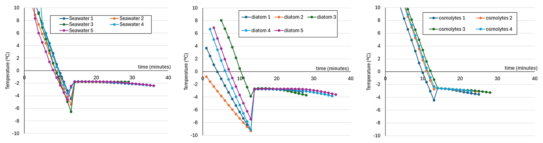
Figure 2 Change in temperature (°C) over time (minutes). Left: artificial seawater growth media (36 PSU Instant Ocean^® with $f/\mathrm{2}$ + Si media) without diatoms, middle: culture of diatoms in artificial seawater, right: supernatant of the diatom in artificial seawater culture, Each panel shows the temperature time series for four to five replicates. Note the initial drop in temperature to a supercooled state, followed by an abrupt increase to the freezing temperature. Data is recorded at 1 min intervals.

4.2 Model: Biofilm Community

Biofilms, suspected to be commonly present in sea ice (Krembs et al., 2002; Roukaerts et al., 2021), are communities of organisms anchored in place by self-secreted extracellular matrices of polymers and other substances (Hall-Stoodley et al., 2004). In environmental settings they are often observed in a pseudo-steady state in which inputs and outputs roughly balance; we approximate sea ice biofilms to be in such a state here, dropping Eqs. (A4)–(A5) and setting $B_{\mathrm{bulk}}(\mathit{x},t)=\mathrm{1}$ in Eq. (A3). The osmolyte production function in Eq. (A3) is defined to be

$$\begin{array}{}\text{(1)}& \begin{array}{rl}& P(S_{\mathrm{brine}},O_{\mathrm{brine}},O_{\mathrm{bulk}},B_{\mathrm{bulk}})\\ & =Y_{\mathrm{osmo}}{r}_{\mathrm{O}}{e}^{-(S_{\mathrm{brine}}+Y_{\mathrm{sal}}{O}_{\mathrm{brine}})/\mathit{\lambda }}{B}_{\mathrm{bulk}}-{\mathit{\gamma }}_{\mathrm{osmo}}{O}_{\mathrm{bulk}}\end{array}\end{array}$$

where λ is a salinity inhibition coefficient, γ_osmo is a decay coefficient, and Y_osmo is a yield coefficient. Production is proportional to bulk microbial concentration with a decay proportional to bulk osmolyte concentration. The exponential encodes production inhibition at high effective salinity measured relative to λ. Production rate coefficient r_O is set at r_O=0.1 h⁻¹ for the computation discussed below. See Appendix C for other parameter values.

See Fig. 3, left column, for results from a representative simulation. To set initial conditions, we simulate “inert” ice, that is, ice without biological activity ($B(z,t)=\mathrm{0}$ and $O_{\mathrm{bulk}}(z,t)=\mathrm{0}$) until an approximate steady state is reached, and use the resulting values of S_bulk and H_bulk as initial (t=0) conditions for the biofilm computation, together with $B(z,\mathrm{0})=\mathrm{1}$. After a transient period due to the abrupt introduction of biological activity, the simulation settles on an approximately periodic behavior with bursts of convective activity in an approximately 10 cm thick layer at the bottom, and an additional tapering flow up to an additional (approximately) 10 cm, Fig. 3 top left. Note also the slow build up of osmolyte in a layer near the top of the convective region, Fig. 3 middle left, where convection is slow due to low ice permeability; this layer eventually discharges as well (not shown). Thickness of the microbially-induced convective layer is limited by low permeability above this layer, which, effectively, does not allow convective draining to proceed fast enough to avoid salinity inhibition (recall the exponential inhibition term in Eq. 1). Non-biologically sourced salinities reach levels similar to osmolyte concentrations, Fig. 3 bottom left, although levels are higher at the bottom where seawater enters the ice.

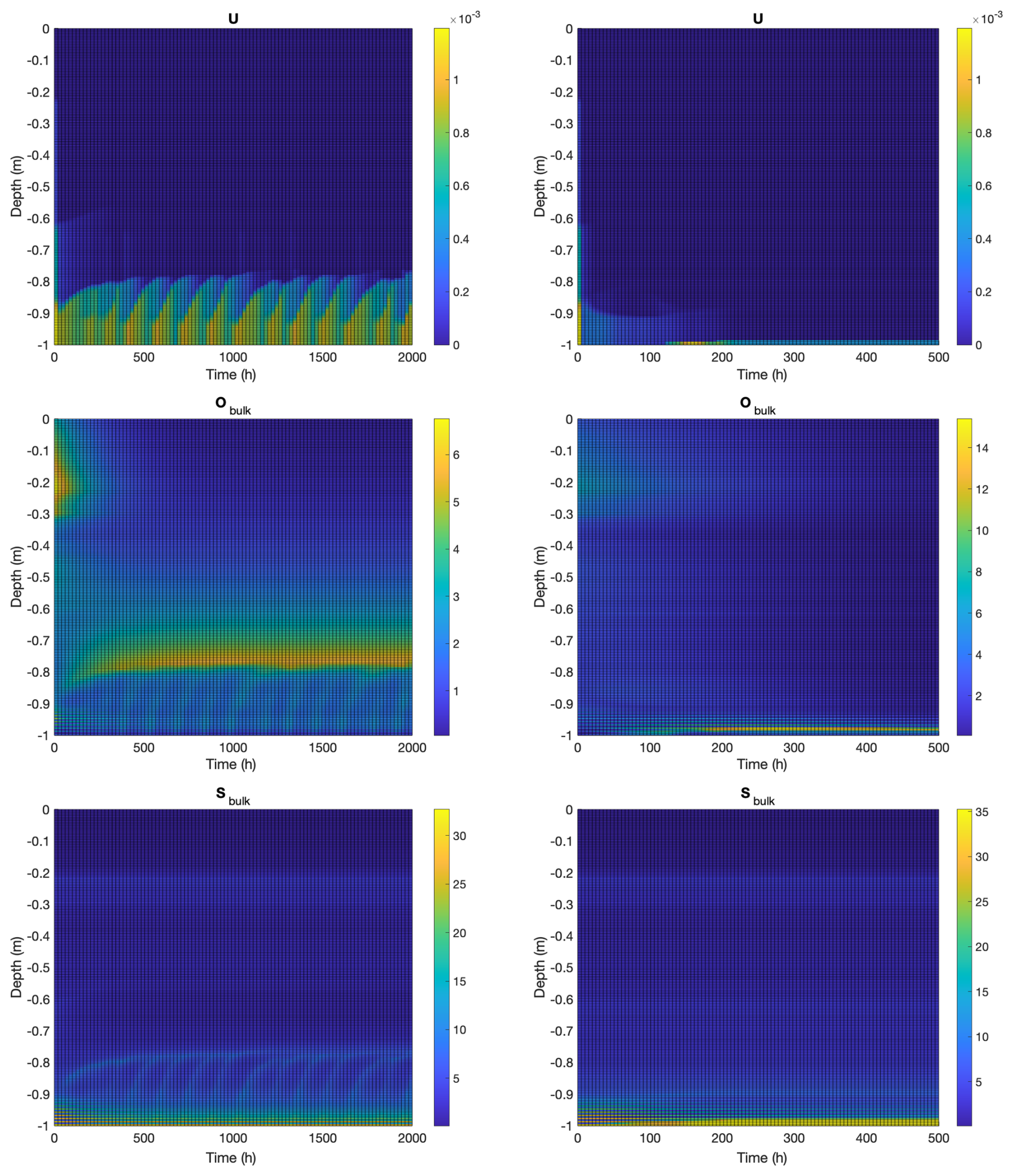
Figure 3 Computational results for a 1 m thick ice column with biofilm population for 2000 h (left) and planktonic population for 500 h (right). Vertical axes indicate depth from the ice-air interface at z=0. Initial conditions for both computations consist of an abiotic system at approximate steady state, with biological perturbation added. Transients seen in the early hours of the simulation are consequences of this transition. Top: vertical velocity (m h⁻¹). Middle: bulk osmolyte concentration (ppt). Bottom: bulk salinity (ppt).

4.3 Model: Planktonic Community

Alternatively, we consider the possibility of a microbial community in a planktonic state, i.e., not ice-attached, and allow this population to advect passively with any present convective flow. The ice column domain is appended with a sea compartment, near but below the ice, from which organisms can advect upward into the ice when the velocity U is non-zero, and into which organisms are ejected from ice regions where Ra exceeds Ra_crit. In addition, we include a nutrient supply, necessary (in the planktonic model) for microorganism growth, that is advectively transported upward into the ice with velocity U from a constant concentration source in the sea compartment. Osmolyte production function P was chosen as in Eq. (1), with r_O=0.2 h⁻¹. Again, see Appendix C for other parameter values. The nutrient usage term R in Eqs. (A4) and (A5) is chosen to be of Monod form, commonly chosen for microbial systems,

$$\begin{array}{}\text{(2)}& R(S_{\mathrm{brine}},O_{\mathrm{brine}},C_{\mathrm{brine}})=r_B{\displaystyle \frac{C_{\mathrm{brine}}}{K+C_{\mathrm{brine}}}}{e}^{-(S_{\mathrm{brine}}+Y_{\mathrm{sal}}{O}_{\mathrm{brine}})/\mathit{\lambda }},\end{array}$$

where K is a half-saturation (set to a large value in order to maintain first-order nutrient kinetics). The exponential term is the same effective salinity inhibition factor as in Eq. (1), for consistency. That is, inhibition of microbial activity is assumed to affect osmolyte production and nutrient usage equally. See Appendix A6 for additional details. Note that we did not see a significant nutrient depletion in the results, though, even with K large enough so that first order kinetics were maintained. This is likely in part due to ice formation inducing brine concentration. Also note that the presence of nutrients in sea ice, in the layer near the interface with the sea, has been reported to be correlated with high biomass concentrations, referred to in Roukaerts et al. (2021) as the sea-ice nutrient paradox. Here the association arises as a consequence of microbially-induced convection.

Initial conditions are set as in the biofilm model computation described in Sect. 4.2, except with $B_{\mathrm{bulk}}(z,\mathrm{0})=\left|z\right|/L$. This form of the initial biomass, with microbes concentrated more towards the ice-sea interface, is so as to allow the microbes a chance to form and sustain a convective layer. It also, though roughly, approximates the distribution of microorganisms that might be expected in a developed sea ice column.

The planktonic model is, as is the biofilm model, capable of formation of a convective layer at the bottom of the ice column, though only for sufficiently large rate of osmolyte production – otherwise microorganisms are excluded to the sea compartment only. In fact, setting r_O=0.1 h⁻¹, as in the biofilm computation, results in washout and no convective layer persisting. See Fig. 3, right column, for a representative simulation with r_O=0.2 h⁻¹ and resulting convective layer formation. Results are different in some important ways from those in the biofilm example. Note that an approximately 3–5 cm thick, steady convective layer forms at the very bottom of the ice column, with thickness here determined largely by the Rayleigh condition through the height h (see Eq. A14) of the top of the layer. That is, the top of the convective layer occurs approximately where the gravitational potential energy, from increased density, and decreased fluid viscosity, from increased permeability, is sufficient so as to trigger a convective instability. Because microorganisms advect with flow, unlike in the biofilm case, they then wash out back into the sea compartment. That is, in the planktonic model, microorganisms can only penetrate ice where upward flow advects them, whereas in the biofilm case, organisms can sit in non-convective ice regions, for a time, producing osmolyte until concentrations become large enough to trigger fluid instability, thus allowing, periodically, a significantly thicker advective layer.

4.4 Model: Transport Effects

Change in temperature $T(z,t)-T(z,\mathrm{0})$ is shown in Fig. 4. This quantity is the difference between the ice temperature, with biofilm of planktonic populations (at time t) and the temperature of the initial t=0 ice column approximate steady state, computed without biofilm (left) or planktonic (right) populations. In the biofilm case (left), as might be expected, temperature increases in the convective layer due to the influx of relatively warm seawater. Perhaps less expectedly, temperature above the convective layer actually decreases with introduction of biofilm activity. This seems to be a consequence of an increase in brine volume fraction there due to osmolyte production, which results in a drop in thermal conductivity, see Appendix A1. Note, as a consequence, heat flux density $-k(\partial /\partial z)T$ through the non-convective part of the ice column is reduced (thermal diffusivity k is nearly unchanged in the upper parts of the column since there is very little osmolyte present there). That is, the model predicts microbial activity can reduce heat transport through the ice a bit, despite advective transport in the convective layer. This prediction, though, may be dependent on model assumptions such as the form of the salinity inhibition factor in Eq. (1), and also may be overestimated since the liquidus relation used in computations tends to overestimate brine volume fraction at lower temperatures (see Appendix A3). In the planktonic model case (right), the temperature increment $T(z,t)-T(z,\mathrm{0})$ is negative throughout the ice column, even in the convective layer, again apparently as a consequence of an increase in brine volume fraction due to osmolyte production, which results in a drop in thermal conductivity. As in the biofilm model case, heat flux density through the non-convective part of the ice column is reduced.

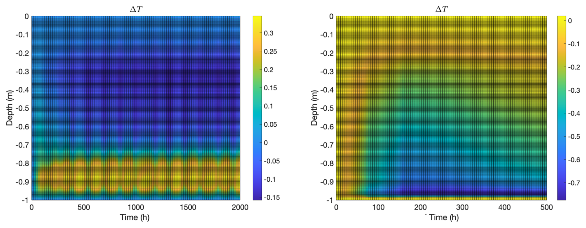
Figure 4 Temperature change $T(z,t)-T(z,\mathrm{0})$ after addition of microbes for the same computations as in Fig. 3, again with biofilm population for 2000 h (left) and planktonic population for 500 h (right). Vertical axes indicate depth from the ice-air interface at z=0. In the biofilm case, (1) temperature increases in the convective region because of inflow of relatively warm seawater and (2) temperature decreases in the mid-ice region likely because of smaller diffusivity (due to increased brine volume fraction). In the planktonic case, temperature decreases throughout the ice column, although the decrement is relatively small in the thin convective region at the bottom of the column.

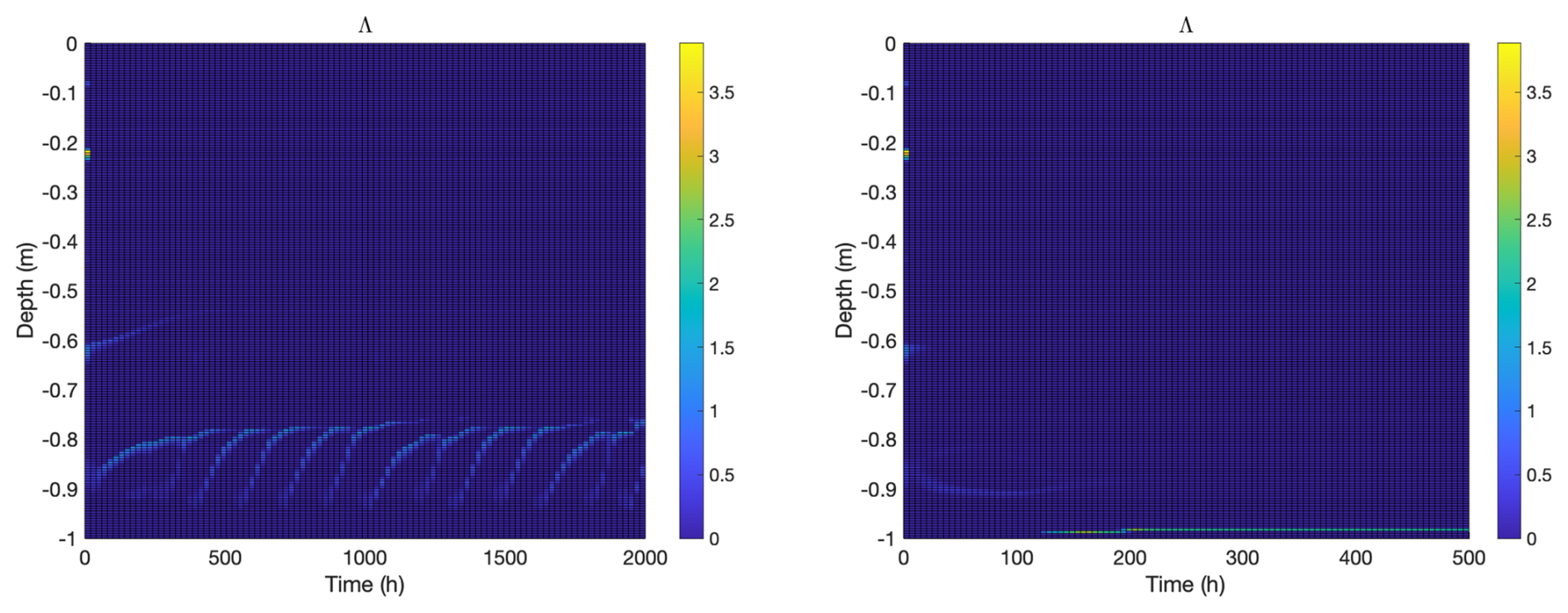
Figure 5 shows a plot of the ratio Λ of outflux to osmolyte production, $\mathrm{\Lambda }=\mathit{\alpha }max(\mathrm{0},\mathit{Ra}-{\mathit{Ra}}_{\mathrm{crit}})/P$, see Eqs. (A3) and (A16), for both the biofilm and planktonic model computations. Note that in both cases, the flows seen in Fig. 3 are largely driven by thin layers where the Rayleigh condition Ra>Ra_crit is satisfied. It is also interesting to note that, in these layers, the ratio Λ≈1 suggesting that the flow rate is effectively determined by the osmolyte production rate. That is, microorganisms can regulate the flow rate through the ice (and hence nutrient supply and byproduct expulsion) by their osmolyte production rate. This is not surprising: if flow rate is smaller than osmolyte production rate, then osmolyte will accumulate which will increase permeability, leading to higher flow rate, and vice-versa in the case that flow rate is higher than osmolyte production rate. In this way the ice community can function something like a self-regulated chemostat: by setting the osmolyte production rate, they also set the convective flux rate and, as a consequence, the rates of inflow of nutrients and outflow of byproducts.

Figure 5 The ratio $\mathrm{\Lambda }=\mathit{\alpha }max(\mathrm{0},\mathit{Ra}-{\mathit{Ra}}_{\mathrm{crit}})/P$ for the two computations shown in Figs. 3 and 4. In both cases, flow is caused by thin regions, where Λ≈1, that drive Rayleigh-Taylor convection, suggesting that microbes can control convective transport rate through osmolyte production P.

In the context of transport, it is also interesting to look at microbially-induced changes in ice permeability, see Fig. 6. Permeability relates flow rate through a material to flow driving force, see Darcy's Eq. (A13), and thus is the central material property for understanding fluid flow through sea ice. We see significant impacts on ice structure in both the biofilm and planktonic cases. Microbes, at least as predicted by the model presented here, can produce qualitative changes in ice structure with regards to fluid flow properties, and do this simply through production of osmolytes. Changing the local effective salinity regulates brine volume fraction, which is an important regulator for permeability, which in turn is an important regulator for transport rate of nutrients and byproducts. (As a side remark, we note that model results appear to be rather insensitive to choice of permeability model as a consequence of osmolyte accumulating until permeability triggers flow, regardless of choice of permeability model.)

The two model cases are different, though. “Biofilm” ice permeability exhibits the same temporal periodicity as observed in the induced convective flow (the activity bursts in Fig. 6, left panel, match well with those in Fig. 3, top left panel), but note that smaller permeability changes also occur well into the ice column, following biofilm activity. Permeability changes in “planktonic” ice are limited to a small bottom layer where microbes are found. On the other hand, permeability levels in that layer are relatively large, due in large part to active convection of warm ocean water. Note that permeability impacts actually spread beyond the convective regions, in both cases, largely because the harmonic averaging used in formula (A15) is somewhat blurring in nature.

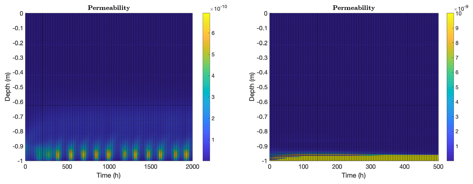
Figure 6 Ice permeability (m²), computed as in formula (A15), for the same computations as in Fig. 3, again with biofilm population for 2000 h (left) and planktonic population for 500 h (right). Vertical axes indicate depth from the ice-air interface at z=0. In the biofilm case, permeability exhibits periodic bursts corresponding to the convective activity shown in Fig. 3 (top left), with smaller permeability changes also occurring higher in the ice column. In the planktonic case, permeability changes are limited to a thin bottom layer where microbes reside, though permeability levels there are relatively large due to active convection of warm ocean water.

5 Conclusions

We have proposed a mechanism for induced convective flow within sea ice, based on microbial osmolyte production. The underlying idea is relatively simple: sea ice organisms produce osmolytes that increase local effective salinity, which in turn increases local brine volume fraction thus opening the ice to fluid flow. This effect is passively and stably self-regulating: fluid flow rate through the ice must match, on average, osmolyte production rate. If not, overly slow fluid flow would allow osmolytes to accumulate which further increases ice permeability, while overly fast fluid flow would flush osmolytes too fast and thus would lower permeability. As a consequence, we suggest that microbes, through production of osmolytes or substances with osmolytic properties, can induce and control continuing convection in a bottom layer of sea ice by themselves, essentially, even after inorganic salt would have largely drained out of biologically inert ice.

The hypothesis is supported first via a study of a C. neogracilis culture, a diatom observed in the field in sea ice, for which we measured a decrease in the freezing point of approximately 1 °C from an abiotic model of seawater, even from culture supernatant. Although the in situ microbial community is rarely monospecific, this particular species is frequently reported as dominant, e.g., Katsuki et al. (2009); Crawford et al. (2018). Note, though, that we only performed short-term measurements (30–40 min) using only lab cultured organisms, reducing opportunities for adaptation and acclimation, and conditions closer to those found in situ may produce a different response. So, while the results are suggestive, further studies looking at, for example, other species or species assemblages, the composition and role of osmolytes, and the direct role of cells on the freezing point are still needed.

Secondly, we present a mathematical model, an augmented version of a previous, abiotic one for density-driven salt draining that relies on entrainment of new seawater via advancing ice column growth. The new mathematical model includes simple representations of both biofilm and planktonic microbial communities and production of osmolyte. In support of the hypothesis, we observe sustained density-driven convective flow through the mechanism described above. That is, the model predicts osmolyte-driven convection in a bottom of a layer of sea ice. While the model simplifies what are likely complicated fluid dynamics, and we cannot rule out result dependence on those simplifications, the underlying mechanism nevertheless seems robust; microbial osmolyte production can eventually increase ice permeability until advective flow is triggered, and the two should balance over time. An additional note: the model predicts that biofilms, i.e., ice-attached organisms, increase the advective layer thickness in comparison to planktonic ones, as planktonic organisms tend to be washed out by the advection. While this observation may again depend on details of the fluid mechanics, it seems plausible, as sessile organisms would be most dependent on sustained brine advection.

We have focused on supporting the possibility of microbially-driven convective flow via osmolyte production, and arguing its mechanistic robustness. More quantitative predictions, e.g., thicknesses of convective layers, are likely generally dependent on parameter choices at least some of which are uncertain, e.g., osmolyte production rate r_O and osmolyte salinity yield Y_sal. Though to the extent possible we attempt to choose reasonable values, and we note that quantitative predictions in turn appear reasonable, nevertheless we would be cautious about interpretations of such results. This is already true within the constraints of the 1D model, even before considering the significant simplifications made in constructing it. It is also worth noting that we assume a steady environment for the purposes of demonstrating that the model can predict constant or, in the biofilm case, periodic behavior induced by microbial activity. Even leaving aside model predictions, the actual sea ice environment is far from steady, exhibiting temperature variations on various time scales, for example. Mechanical stressing by the underlying sea dynamics, not included in the model, is also likely to have significant impact. Also notable, we apply set initial conditions using a pre-simulation of an established, non-advecting (abiotic) ice column, thus imitating to an extent a winter-spring transition from biologically inactive to biologically active ice. This differs from what one might expect in the late fall during formation of first year ice, where a microbially-induced convective layer would form along with the growing ice column. We did not investigate this latter possibility here because of its coupling with ice column growth, which introduces additional complications that can obscure the main point. Nevertheless, we would expect that a similar microbially-influenced convective layer could be present, at least in model simulations.

Results suggest plausibility of significant microbial impact on sea ice structural and material properties, beyond albedo effects, even though the presentation here is conservative in some ways. Notably, we impose a relatively large 18ºC temperature difference between the air and ocean interfaces to argue robustness. This localizes effects to the bottom of the ice column, but for less extreme temperature differences it may be possible, even, for microbes to open channels and maintain activity through the entire ice column, which could have important implications on sea ice both as a microbial habitat and also as a nutrient cache. Indeed, recent observations support this possibility (Audh et al., 2023). Any impacts on brine channel microstructure, and induced thermal transport can impact thermal transport as well (Kraitzman et al., 2024). On another note, model results suggest the possibility of significant amounts of microbially produced osmolyte. Indeed, as an example, high concentrations of DMSP and DMS have been observed in sea ice environments, and their biological origins has attracted attention of astrobiologists (Madhusudhan et al., 2025).

In the broader picture, moving from static sea ice models to dynamic, mushy-layer sea-ice in climate models has shown significant influence on results, including increasing snow-ice and coastal ice production as well as enhancement of surface ocean salinity due to brine rejection (Turner and Hunke, 2015; Bailey et al., 2020; Singh et al., 2021; DuVivier et al., 2021), and also more accurate predictions of both low-level cloud cover around Antarctic coasts and atmospheric energy input (DuVivier et al., 2021). Results reported here suggest that including biological processes, specifically microbial modification of ice properties, may also merit attention.

Appendix A: Equations

A1 Conserved Scalar Fields

The model equations are largely standard (although we track bulk enthalpy H_bulk rather than, directly, temperature T, following Notz (2005); Griewank and Notz (2013)) except with the addition of transport equations for osmolyte, nutrient, and biomass concentrations (O_bulk, C_bulk, and B_bulk respectively). These quantities are governed by transport equations

$$\begin{array}{}\text{(A1)}& {\displaystyle \frac{\partial }{\partial t}}\left(\mathit{\rho }{H}_{\mathrm{bulk}}\right)=-\mathrm{\nabla }\cdot \left(\mathit{\rho }{H}_{\mathrm{brine}}\mathit{U}\right)+\mathrm{\nabla }\cdot \left(k\mathrm{\nabla }T\right),\text{(A2)}& {\displaystyle \frac{\partial }{\partial t}}{S}_{\mathrm{bulk}}=-\mathrm{\nabla }\cdot \left(S_{\mathrm{brine}}\mathit{U}\right)+\mathrm{\nabla }\cdot \left({\mathit{\kappa }}_S\mathrm{\nabla }{S}_{\mathrm{brine}}\right),\text{(A3)}& {\displaystyle }\begin{array}{rl}{\displaystyle \frac{\partial }{\partial t}}{O}_{\mathrm{bulk}}& =-\mathrm{\nabla }\cdot \left(O_{\mathrm{brine}}\mathit{U}\right)+\mathrm{\nabla }\cdot \left({\mathit{\kappa }}_{\mathrm{O}}\mathrm{\nabla }{O}_{\mathrm{brine}}\right)\\ & +P(S_{\mathrm{brine}},O_{\mathrm{brine}},C_{\mathrm{brine}},B_{\mathrm{bulk}}),\end{array}\text{(A4)}& {\displaystyle }\begin{array}{rl}{\displaystyle \frac{\partial }{\partial t}}{C}_{\mathrm{bulk}}& =-\mathrm{\nabla }\cdot \left(C_{\mathrm{brine}}\mathit{U}\right)+\mathrm{\nabla }\cdot \left({\mathit{\kappa }}_C\mathrm{\nabla }{C}_{\mathrm{brine}}\right)\\ & -R(S_{\mathrm{brine}},O_{\mathrm{brine}},C_{\mathrm{brine}})B_{\mathrm{bulk}},\end{array}\text{(A5)}& {\displaystyle }\begin{array}{rl}{\displaystyle \frac{\partial }{\partial t}}{B}_{\mathrm{bulk}}& =-\mathrm{\nabla }\cdot \left(B_{\mathrm{brine}}\mathit{U}\right)+\mathrm{\nabla }\cdot \left({\mathit{\kappa }}_B\mathrm{\nabla }{B}_{\mathrm{brine}}\right)\\ & +\left(Y_{B}R\right(S_{\mathrm{brine}},O_{\mathrm{brine}},C_{\mathrm{brine}})-{\mathit{\gamma }}_B)B_{\mathrm{bulk}},\end{array}\end{array}$$

where k is a thermal diffusivity and the various κ's are material diffusivities. Yield coefficient Y_B translate substrate usage into production of new biomass, and γ_B is a microbial decay rate. Functions P and R are osmolyte production and limiting nutrient reaction terms, respectively, discussed further below, with examples of particular choices given in Eqs. (1) and (2) respectively. Note that both can be inhibited at sufficiently high concentrations of salt and osmolyte, as a result of microbial activity inhibition. The last term in Eq. (A5) is the net biomass growth term, with growth term Y_BR supposed proportional to nutrient uptake R and including first order decay with rate γ_B. Definitions for bulk and brine quantities are discussed below.

We neglect the diffusion terms in Eqs. (A2)–(A5), as is common practice for an ideal mushy layer (Worster, 1992, 1997). Velocity U is discussed below. The thermal conductivity depends on brine volume fraction ϕ_brine, which we approximate in volume averaged form as $k=k_{\mathrm{b}}{\mathit{\varphi }}_{\mathrm{brine}}+k_{\mathrm{i}}(\mathrm{1}-{\mathit{\varphi }}_{\mathrm{brine}})$ where k_b, k_i are the thermal conductivities in brine and ice, respectively. Note that k_i is roughly a factor of 10 larger than k_b (Kannuluik and Carman, 1951; Yen, 1981; Thomas and Dieckmann, 2008), so that an increase in brine volume fraction ϕ_brine results in decreased thermal conductivity. Density ρ in Eq. (A1) is also in principle a weighted average over brine and ice densities, but we neglect the difference between the two densities (approximately 10 %), again as is frequently done (Worster, 1997). A consequence of this supposition is that we can impose $\mathrm{\nabla }\cdot \mathit{U}=\mathrm{0}$.

Equations (A2)–(A5) take no-flux boundary conditions at the ice-air interface (i.e., normal derivatives across the interface are zero), and, at the ice-ocean interface, flux is set to the inflowing advective flux, e.g. S_seaU⋅n for Eq. (A2) where n is an in-pointing interface normal vector. Equation (A1) takes Dirichlet boundary conditions using Eq. (A9) together with given values for air and sea temperatures ($T=-\mathrm{20}$ °C and $T=-\mathrm{2}$ °C, respectively). Note that these conditions depend on brine volume fraction ϕ_brine, but are approximated here using ϕ_brine=1 at the ice-ocean interface and ϕ_brine=0 at the ice-air interface.

A2 Salinities and Volume Fractions

Seawater is a solution of water and many salt species, as well as other dissolved and undissolved contaminants, but we simplify by dividing into water, microbially produced antifreeze chemicals (e.g., DMSP) lumped together under the designation “osmolyte”, and other dissolved chemical species lumped together under the designation “salt”. Undissolved contaminants, e.g., microbial cells, extracellular polymers, etc., are neglected here though could effect freezing properties. In a unit control volume V, we define (partial) bulk salt and osmolyte salinities (ppt) as

$$\begin{array}{c}{\displaystyle }{S}_{\mathrm{bulk}}={\displaystyle \frac{m_{\mathrm{salt}}}{m_{\mathrm{water},\mathrm{\ell }}+m_{\mathrm{water},\mathrm{s}}}}\times {\mathrm{10}}^{-\mathrm{3}}\mathrm{ppt},\\ {\displaystyle }{O}_{\mathrm{bulk}}={\displaystyle \frac{m_{\mathrm{osmo}}}{m_{\mathrm{water},\mathrm{\ell }}+m_{\mathrm{water},\mathrm{s}}}}\times {\mathrm{10}}^{-\mathrm{3}}\mathrm{ppt},\end{array}$$

where m_salt and m_osmo are the control volume masses of salt and osmolyte respectively, and m_water,ℓ and m_water,s are the control volume masses of liquid water and ice, respectively. Then (partial) brine volume fractions are defined as

$$\begin{array}{c}{\displaystyle }{S}_{\mathrm{brine}}={\displaystyle \frac{m_{\mathrm{salt}}}{m_{\mathrm{water},\mathrm{\ell }}}}\times {\mathrm{10}}^{-\mathrm{3}}\mathrm{ppt}={\mathit{\varphi }}_{\mathrm{b},\mathrm{m}}^{-\mathrm{1}}{S}_{\mathrm{bulk}},\\ {\displaystyle }{O}_{\mathrm{brine}}={\displaystyle \frac{m_{\mathrm{osmo}}}{m_{\mathrm{water},\mathrm{\ell }}}}\times {\mathrm{10}}^{-\mathrm{3}}\mathrm{ppt}={\mathit{\varphi }}_{\mathrm{b},\mathrm{m}}^{-\mathrm{1}}{O}_{\mathrm{bulk}},\end{array}$$

where

$${\mathit{\varphi }}_{\mathrm{b},\mathrm{m}}={\displaystyle \frac{m_{\mathrm{water},\mathrm{\ell }}}{m_{\mathrm{water},\mathrm{\ell }}+m_{\mathrm{water},\mathrm{s}}}}$$

is the brine mass fraction. Note that we are neglecting m_salt and m_osmo contributions to total mass as small. Finally, we define ϕ_brine to be the brine volume fraction, i.e., the ratio of brine volume to total volume in the unit control volume, and make the approximation ${\mathit{\varphi }}_{\mathrm{brine}}={\mathit{\varphi }}_{\mathrm{brine},\mathrm{m}}$.

These definitions, written in terms of mass, can also be written in terms of densities by multiplying the right-hand side by $V^{-\mathrm{1}}/V^{-\mathrm{1}}$, where V is a unit volume. Also note that, with the approximate equivalence of liquid and ice water volume, the quantity $V^{-\mathrm{1}}(m_{\mathrm{water},\mathrm{\ell }}+m_{\mathrm{water},\mathrm{s}})$ can be considered constant (in both space and time), and hence S_bulk and O_bulk are, approximately, functions of salt and osmolyte concentrations only. A similar observation holds for volume fraction ϕ_brine.

A3 Liquidus Relations

Solvent (here water) freezing temperature is generally lowered in the presence of a solute – briny water has a lower freezing point than pure water. Freezing temperature and brine salinity in a simple solution (a solution with a single solvent species) have been connected through a so-called liquidus relation S_brine=ℒ(T) (Worster, 1992, 1997; Feltham et al., 2006; Wells et al., 2011, 2019) where T is freezing temperature at concentration S_brine. Abiotic seawater is often approximated in this context as a simple solution of water and generic “sea salt” though seawater is more complicated, even without considering its insoluble component. A liquidus relation can still be applied, though it depends on the nature of the solution, and approximations of it have been constructed for seawater as a function of salinity (Notz, 2005).

The liquidus function ℒ is generally determined empirically for a given solution. For computations, we use here a linear approximation

$$\begin{array}{}\text{(A6)}& \mathcal{L}\left(T\right)=-T/\mathrm{0.05411}\end{array}$$

which generally works well for seawater at temperatures near or above −6 °C, approximately; for lower temperatures; Eq. (A6) overestimates brine concentration (Notz, 2005), but the effect on results here is small because ice permeability is too low, even with more accurate liquidus approximations, to allow significant flow channels to occur in regions with low temperatures.

Microbes are able in certain cases to produce osmolytic compounds to protect themselves from freezing. We suppose that these osmolytes can be found extracellularly, though we don't distinguish between active and passive (e.g., through cell lysing) excretion. For reference, note the reported wide-spread and significant concentrations of the compound DMSP associated with antarctic ocean algae and cyanobacteria communities – we aren't aware of evidence that it is, or isn't, actively excreted, but it has been measured in large concentrations regardless. To introduce effects of microbes, we divide solutes into two types, abiotic (e.g., inorganic salts) and biotic. In fact, nonsoluble biotic contaminants might also impact freezing temperature, but are not separately considered. That is, we consider a brine system with two solute types, one of which is subject to microbial control.

Extension of the liquidus relation to two (or more) solute types requires a short computation, as follows. Denoting abiotic and biotic concentrations by S_brine and O_brine respectively, we use the liquidus approximation as in the abiotic case in the form

$$\begin{array}{}\text{(A7)}& S_{\mathrm{brine}}+Y_{\mathrm{sal}}{O}_{\mathrm{brine}}=\mathcal{L}\left(T\right)\end{array}$$

where Y_sal is a salinity yield coefficient. That is, we don't assume that the biotic osmolyte has the same effect on freezing point, per mass, as the abiotic one. Note then the pointwise requirement $S_{\mathrm{brine}}/O_{\mathrm{brine}}=S_{\mathrm{bulk}}/O_{\mathrm{bulk}}$, together with Eq. (A7), results in the pair of liquidus-like relations

$$\begin{array}{}\text{(A8)}& \begin{array}{rl}{O}_{\mathrm{brine}}& ={\displaystyle \frac{O_{\mathrm{bulk}}}{S_{\mathrm{bulk}}+Y_{\mathrm{sal}}{O}_{\mathrm{bulk}}}}\mathcal{L}\left(T\right),\\ S_{\mathrm{brine}}& ={\displaystyle \frac{S_{\mathrm{bulk}}}{S_{\mathrm{bulk}}+Y_{\mathrm{sal}}{O}_{\mathrm{bulk}}}}\mathcal{L}\left(T\right).\end{array}\end{array}$$

Note 1. The value of the salinity yield Y_sal is unknown (and, indeed, effective salinity is an introduced idea here). Based on the results of Sect. 4.1, we suppose, lacking other measurements, that biologically-induced osmolyte is relatively effective in comparison to abiotic salinity and so have set Y_sal=5 in computations. Note that we have not observed significant qualitative differences for other O(1) choices of Y_sal in computations.

Note 2. The liquidus relation (A6) is an empirical one, intended for seawater relatively near to −1.8 °C in temperature. We don't know how accurate it is when osmolyte is included as in Eq. (A7), even in this same temperature range, as we don't have available a liquidus relation for the combined seawater plus microbially-produced osmolyte system. This is another reason to be cautious particularly about quantitative model predictions.

A4 Formulas for Brine Volume Fraction and Concentrations

We divide the various fields by slow and fast time scales. Bulk conserved quantities H_bulk, S_bulk, O_bulk, C_bulk, B_bulk are governed by Eqs. (A1)–(A5), and change on the relatively slow diffusive and advective time scales. Locally, it is commonly assumed that an ice-brine balance, consistent with liquidus relations (A8), is approached on a much faster time scale. That is, relations (A8) are imposed as constraints. Additionally, enthalpy and temperature are related by the approximation (Notz, 2005)

$$\begin{array}{}\text{(A9)}& H_{\mathrm{bulk}}=c_{s}T-(\mathrm{1}-{\mathit{\varphi }}_{\mathrm{brine}})L_{\mathrm{0}},\end{array}$$

where c_s is ice heat capacity, approximated to be a constant, independent of temperature and salinity, and L₀ is the latent heat of fusion. Note that $H_{\mathrm{bulk}}{|}_{T=\mathrm{0}}=\mathrm{0}$. Lastly, assuming that the ice phase is pure water, then

$$\begin{array}{}\text{(A10)}& \begin{array}{rl}{S}_{\mathrm{bulk}}& =S_{\mathrm{brine}}{\mathit{\varphi }}_{\mathrm{brine}},\\ O_{\mathrm{bulk}}& =O_{\mathrm{brine}}{\mathit{\varphi }}_{\mathrm{brine}},\\ B_{\mathrm{bulk}}& =B_{\mathrm{brine}}{\mathit{\varphi }}_{\mathrm{brine}}.\end{array}\end{array}$$

Combining these relations with Eq. (A7), we obtain

$$\begin{array}{}\text{(A11)}& {\displaystyle }{\mathit{\varphi }}_{\mathrm{brine}}={\displaystyle \frac{S_{\mathrm{bulk}}+Y_{\mathrm{sal}}{O}_{\mathrm{bulk}}}{\mathcal{L}\left(T\right)}}\text{(A12)}& {\displaystyle }{H}_{\mathrm{bulk}}=c_{s}T-L_{\mathrm{0}}+L_{\mathrm{0}}{\displaystyle \frac{S_{\mathrm{bulk}}+Y_{\mathrm{sal}}{O}_{\mathrm{bulk}}}{\mathcal{L}\left(T\right)}}\end{array}$$

Given H_bulk, S_bulk and O_bulk, the nonlinear Eq. (A12) is solved for T, and then Eq. (A11) for ϕ_brine, and then relations (A10) can be used to compute brine concentrations.

A5 Velocity

Dynamics within the sea ice are commonly modeled via a Darcy flow formulation (Worster, 1992)

$$\begin{array}{}\text{(A13)}& \mathit{\mu }\mathit{U}=\mathrm{\Pi }(-\mathrm{\nabla }p+(\mathit{\rho }-{\mathit{\rho }}_{\mathrm{0}}\left)\mathit{g}\right)\end{array}$$

where μ is the dynamic viscosity, $\mathit{g}=-g\widehat{\mathit{z}}$ (g is the gravitational constant), ρ₀ is a reference density (e.g., density of seawater just below the ice layer), Π is the sea ice permeability, and p and U are pressure and velocity, respectively. Pointwise ice permeability Π is modeled as $\mathrm{\Pi }=\mathrm{\Pi }\left({\mathit{\varphi }}_{\mathrm{brine}}\right)={\mathrm{\Pi }}_{\mathrm{0}}{\mathit{\varphi }}_{\mathrm{brine}}^{\mathrm{3}}$, although an average is used, see Eq. (A15) below. The velocity field U, with units of length per time, can be understood in the context of Darcy flow as volume flux, with units of volume per time per area, obtained by averaging over a local flux surface through a porous medium.

Darcy flow is in fact not applied here. Rather, we follow a parameterized flow model (Griewank and Notz, 2013; Turner et al., 2013; Griewank and Notz, 2015) in which it is supposed that convective flow, induced by a buoyancy driven Rayleigh-Taylor instability, can occur in the ice column. Presence/absence of such a flow is determined by the Rayleigh number Ra (see Sect. A6), which can be defined to be the ratio of two time scales:

1. Diffusive time scale t_D is the time scale for diffusive transport of heat from sea to local brine, approximately $t_{\mathrm{D}}=h^{\mathrm{2}}/\mathit{\kappa }$, where $\mathit{\kappa }=k/c\mathit{\rho }$ is the thermal diffusivity and h is the height above the ice-sea interface. Note: diffusive transport of heat, rather than salt, is appropriate here, as heat diffuses much more quickly and can reduce salinity by melting ice.

2. Convective time scale t_C is the time scale for local brine, at height h above sea, to reach the ocean by buoyancy-driven flow. Darcy flow speed is estimated as $g\mathrm{\Delta }\mathit{\rho }\mathrm{\Pi }/\mathit{\mu }$ where Δρ is density difference between local brine and seawater, so that $t_{\mathrm{C}}=h\mathit{\mu }/\left(\mathrm{\Pi }g\mathrm{\Delta }\mathit{\rho }\right)$.

We then define a local Rayleigh number Ra as the nondimensional ratio

$$\begin{array}{}\text{(A14)}& \mathit{Ra}={\displaystyle \frac{t_{\mathrm{D}}}{t_{\mathrm{C}}}}={\displaystyle \frac{g\mathrm{\Delta }\mathit{\rho }\mathrm{\Pi }h}{\mathit{\kappa }\mathit{\mu }}}={\displaystyle \frac{gc\mathit{\rho }\mathrm{\Delta }\mathit{\rho }\mathrm{\Pi }h}{k\mathit{\mu }}}\end{array}$$

where Δρ is the density difference between local brine and seawater. Permeability Π=Π(x) is spatially variable. We follow here the recommendation in Rees Jones and Worster (2014) and replace Π in our 1D computations by its harmonic average

$$\begin{array}{}\text{(A15)}& {\mathrm{\Pi }}_{\mathrm{harm}}\left(z\right)={\left[{\displaystyle \frac{\mathrm{1}}{z_{\mathrm{0}}-z}}\underset{z}{\overset{z_{\mathrm{0}}}{\int }}{\displaystyle \frac{\mathrm{1}}{\mathrm{\Pi }\left({\mathit{\varphi }}_{\mathrm{brine}}\right(\widehat{z}\left)\right)}}\mathrm{d}\widehat{z}\right]}^{-\mathrm{1}}\end{array}$$

where z₀ is the z coordinate of the sea-ice interface.

We employ a Boussinesq approximation, which suppose ρ constant (again, also neglecting change in density between solid and brine phases) except for buoyancy. That is, ρ is constant except for computation of buoyancy, in which case $\mathit{\rho }={\mathit{\rho }}_{\mathrm{0}}(\mathrm{1}+\mathit{\beta }\mathrm{\Delta }S)$, i.e., Δρ=βρ₀ΔS (where ρ₀ is density at S=0 and β is a buoyancy conversion factor from salinity to density), so

$$\mathit{Ra}={\displaystyle \frac{gc\mathit{\rho }\mathit{\beta }{\mathit{\rho }}_{\mathrm{0}}\mathrm{\Delta }S\mathrm{\Pi }h}{k\mathit{\mu }}},$$

again using Π=Π_harm in our 1D computations. Here S is total “salt”, i.e., $S=S_{\mathrm{brine}}+O_{\mathrm{brine}}$; recall that the osmolyte concentration is normalized so that it has the same density properties as salt (the two are distinguished, rather, by effects on freezing temperatures through the yield Y_sal). Note that there is a conservation of mass issue – osmolyte is, ultimately, generated from material present in the brine, and so new osmolyte might not change brine density. However, osmolyte solute properties likely differ from those of its chemical constituents and so can have different effects on brine density. The inclusion of osmolyte in the total salt S does not appear to have a large effect on results in any case.

A6 Parameterized Convection

The details of flow in sea ice generated by Rayleigh-Taylor instability are complex so instead we follow Griewank and Notz (2013), Turner et al. (2013), Griewank and Notz (2015) and replace the full flow description U in Eq.(A13) used in transport Eqs. (A1)–(A5) with a parameterized model of the form $\mathit{u}(\mathit{x},t)=(\mathrm{0},\mathrm{0},U(z,t\left)\right)$ where

$$\begin{array}{}\text{(A16)}& \begin{array}{rl}& U\left(z\right)=\underset{z_{\mathrm{0}}}{\overset{z}{\int }}\mathrm{\nabla }\cdot \mathit{u}\left(\widehat{z}\right)\mathrm{d}\widehat{z},\\ & \mathrm{\nabla }\cdot \mathit{u}\left(\widehat{z}\right)=\mathit{\alpha }max(\mathrm{0},\mathit{Ra}-{\mathit{Ra}}_{\mathrm{crit}}).\end{array}\end{array}$$

Here z₀ is the z coordinate of the sea-ice interface, and Ra_crit is the critical Rayleigh instability value, see Table C1. Note that u neglects much of the detail of the full flow by only tracking upward velocity. The motivation and intuition is that cold, salty downward flow occurs mostly in relatively large channels (formed because the temperature in colder downflow quickly equilibrates with that in surrounding warmer ice, and then excess salinity causes that surrounding ice to melt) that empty rather directly into the sea below with warmer less salty replacement fluid seeping upwards through surrounding mushy ice, see Fig. A1. The vertical velocity component U(z) accounts, in an averaged sense, for this upward replacement flow.

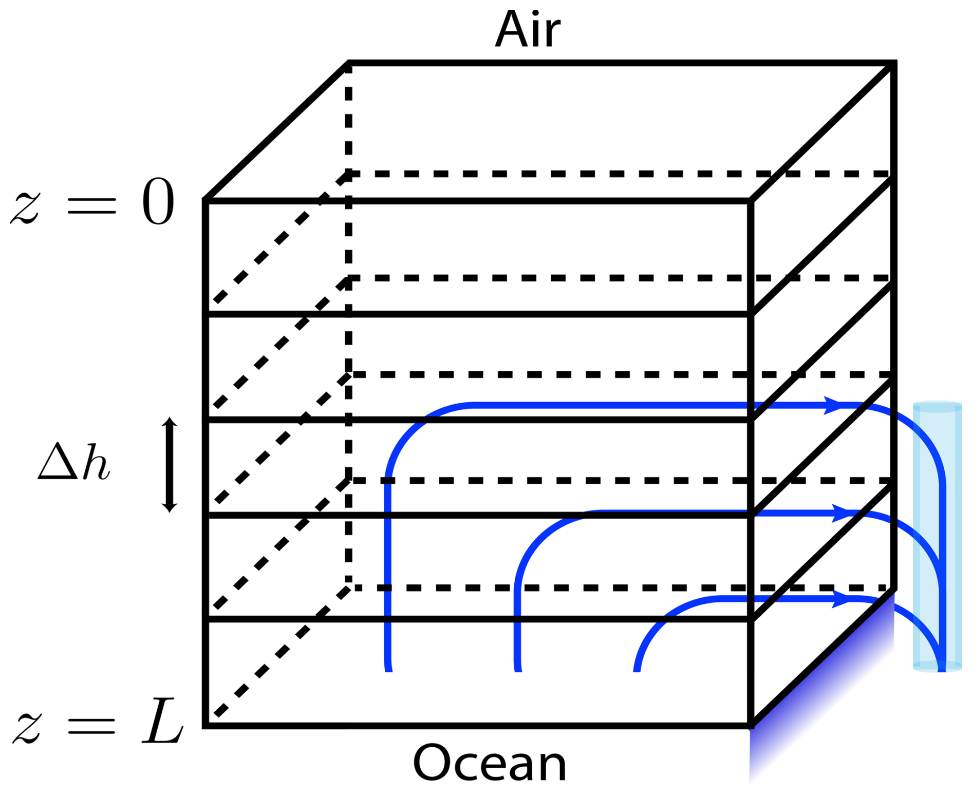
Figure A1 Parameterized flow diagram: flow moves upward (only) to account for drainage. Adaptation from Turner et al. (2013).

When convective flow is present, the planktonic microbial model (recall Sect. 4.3) includes a sea compartment microbe biomass B_sea(t), tracking microbes close to the bottom of the ice column, which receives influx from convectively drained flow according to

$${\displaystyle \frac{\mathrm{d}}{\mathrm{d}t}}{B}_{\mathrm{sea}}\left(t\right)=\underset{\mathrm{0}}{\overset{L}{\int }}{B}_{\mathrm{brine}}(z,t)\mathrm{\nabla }\cdot \mathit{u}\left(z\right)\mathrm{d}z+\mathit{\delta }(B_{\mathrm{sea},\mathrm{0}}-B_{\mathrm{sea}}),$$

where δ is a dilution coefficient. The second term represents mixing between the near ice column organisms and the background, given by constant B_sea,0.

Appendix B: Numerical Methods

Computations are conducted on a 1D domain z∈[0 L], $x,y\in \mathcal{R}$, see Fig. B1. All quantities are assumed to depend spatially only on z, i.e., the system is effectively 1D, with z=0 corresponding to the upper, ice-air interface, and z=L corresponding to the lower, ice-sea interface. The domain is discretized into N uniform subintervals of length Δh (with NΔh=L). In the computations illustrated in Figs. 3–5, we set N=200. Quantities of interest are discretized according to subintervals. Offset discretization is employed for the velocity U and for thermal conductivity, with values taken on subinterval boundaries, while other quantities (enthalpy, temperature, local Rayleigh number, brine volume fraction, and concentrations) are assigned values at each subinterval's midpoint z_i, $\mathrm{1}\le i\le N$. Thermal conductivity on the interface is computed as a harmonic average of the thermal conductivity in the neighboring subintervals, following Notz (2005). Equations (A1)–(A5) are integrated using central differencing for second order terms, and using offset central differencing for advective terms, with first order explicit time integration. Due to use of an explicit method, a small time step $\mathrm{\Delta }t=\mathrm{5}\times {\mathrm{10}}^{-\mathrm{6}}$ h was used.

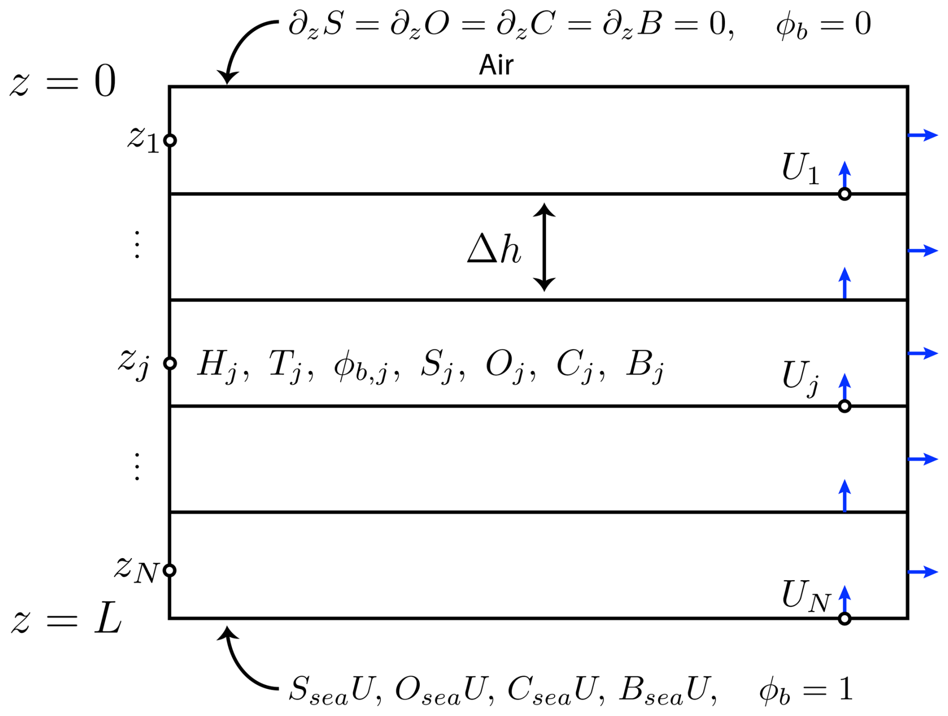
Figure B1 Representation of the computational grid. Velocity and thermal conductivity take values on the interfaces between discretized intervals. Other quantities take values inside the intervals. No-flux and in-flux boundary conditions are indicated, along with Dirichlet conditions for ϕ_brine.

Each iteration consists of the following sequence of computations: given “current” values of each bulk field (the conserved, slowly varying quantities) either from initial conditions or from the previous iteration,

1. Temperature profile is updated using the current enthalpy profile via Eq. (A12).

2. Using the current profile S_bulk+Y_salO_bulk, brine volume fraction is computed using Eq. (A11).

3. Current brine concentration fields S_brine, O_brine, C_brine, and B_brine are computed using Eq. (A10).

4. The local Rayleigh number for each subinterval is updated using the new S_brine profile and Eq. (A14) with, for subinterval i, $h=L-z_i$.

5. The parameterized velocity profile is updated using Eq. (A16).

6. The slow fields H, S_bulk, O_bulk, C_bulk, and B_bulk are updated using discretizations of Eqs. (A1)–(A5).

Initial conditions for abiotic fields are set to be profiles obtained by running the code without microbes and osmolyte to an approximate steady state. Initial conditions for biomass bulk concentration B_bulk are $B_{\mathrm{bulk}}(z,\mathrm{0})=\mathrm{1}$ for the biofilm case and $B_{\mathrm{bulk}}(z,\mathrm{0})=\left|z\right|/L$ for the planktonic case. Initial osmolyte bulk concentrations are $O_{\mathrm{bulk}}(z,\mathrm{0})=\mathrm{0}$ for the biofilm case and $O_{\mathrm{bulk}}(z,\mathrm{0})=\mathrm{5}\left|z\right|/L$ for the planktonic case.

Appendix C: Parameters and Fields

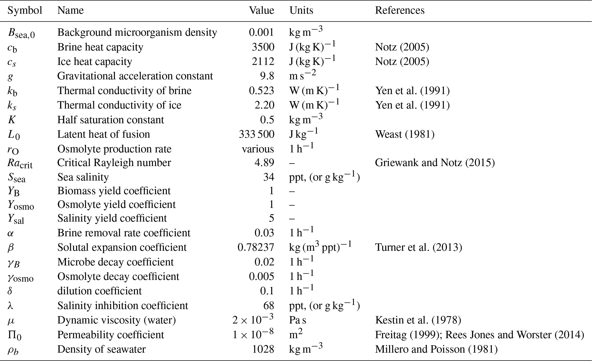
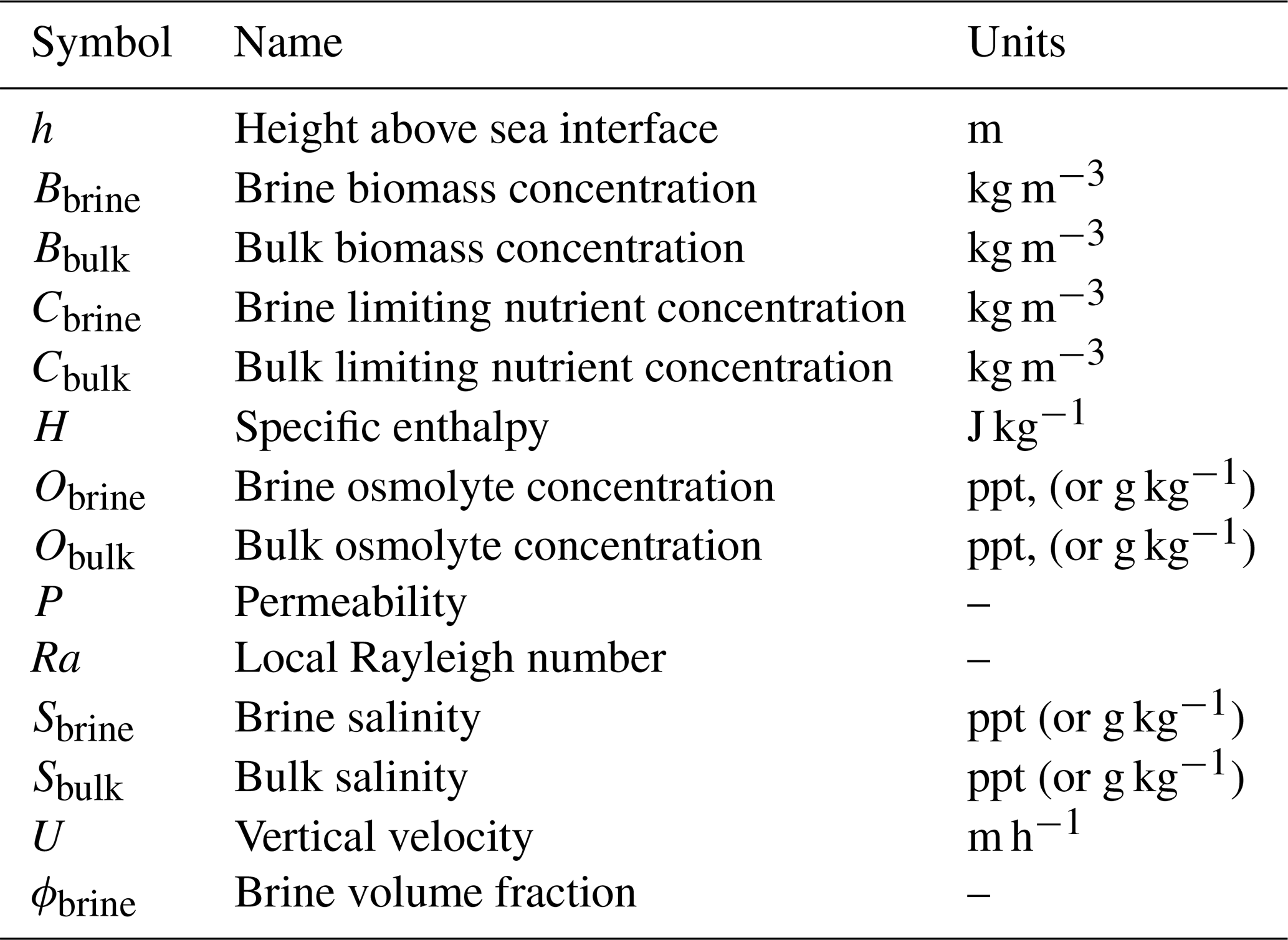
See Table C1 for a list of parameters, and Table C2 for a list of fields.

Notz (2005)Notz (2005)Yen et al. (1991)Yen et al. (1991)Weast (1981)Griewank and Notz (2015)Turner et al. (2013)Kestin et al. (1978)Freitag (1999); Rees Jones and Worster (2014)Millero and Poisson (1981)

Table C1 Model parameters. Some parameters are weakly temperature dependent – we approximate with (constant) values appropriate for seawater temperature.

Table C2 Model fields (all are functions of z and t).