Large regional differences in Antarctic ice shelf mass loss from Southern Ocean warming and meltwater feedbacks

The increasing release of Antarctic meltwater represents one of the most profound, yet uncertain, consequences of global climate change. The absence of interactive ice sheets in state-of-the-art climate models prevents the direct calculation of ice–ocean feedbacks, leaving significant uncertainty in the global and regional consequences of meltwater discharge. This study leverages results from the Southern Ocean Freshwater Input from Antarctica (SOFIA) initiative to assess the ocean response to a 0.1 Sv meltwater perturbation and infer the feedback on ice shelf basal melting across 10 CMIP6 models. We analyze meltwater-induced temperature anomalies across distinct continental shelf regimes and compare them with SSP5-8.5 warming-induced anomalies. We then translate these anomalies into basal melt rates using a parameterization calibrated with a new observational climatology, which reveals strongly regional melt sensitivities that cannot be captured with an Antarctic-wide coefficient. Although the meltwater feedback is generally thought to amplify basal melting, our results demonstrate large regional differences, with implied enhanced ice shelf mass loss in some sectors but suppressed basal melting in others. The model ensemble indicates a warming feedback on the continental shelf in most East Antarctic regions, whereas in West Antarctica, most models simulate either cooling or reduced warming, suggesting a negative feedback. This regional contrast implies that East Antarctica may play an increasingly dominant role in future ice shelf mass loss. Simulations support existing hypotheses linking these asymmetric temperature responses to strong regional connectivity and shelf-break dynamics, including a strengthened Antarctic Slope Front, an accelerated Antarctic Slope Current, and reduced dense shelf water formation.

1 Introduction

The release of Antarctic meltwater represents one of the most profound yet uncertain consequences of future global climate change. Observational evidence reveals that the Antarctic Ice Sheet and its ice shelves are undergoing significant mass loss (Adusumilli et al., 2020; Otosaka et al., 2023; Paolo et al., 2023; Davison et al., 2023, 2025), with the rate of loss accelerating particularly in regions undergoing rapid ice shelf melting (Paolo et al., 2015; Rignot et al., 2019). Projections from standalone ice sheet models indicate that this mass loss will continue to accelerate in response to anthropogenic greenhouse gas forcing (Seroussi et al., 2020, 2024), leading to further increases in meltwater discharge into the Southern Ocean. This mass loss is expected to become the primary contributor to global sea level rise in the coming decades and centuries (Edwards et al., 2021; Fox-Kemper et al., 2021), while associated meltwater also significantly affects regional and global climate (Bronselaer et al., 2018; Fyke et al., 2018; Golledge et al., 2019; Rye et al., 2020; Dong et al., 2022; Purich and England, 2023; Beadling et al., 2024; Fricker et al., 2025; Xu et al., 2025).

Because most coupled climate models, including those in the latest Coupled Model Intercomparison Project (CMIP6, Eyring et al., 2016), do not include fully interactive ice sheets and ice shelves, substantial uncertainty remains about the magnitude (Bamber et al., 2019; Levermann et al., 2020; Edwards et al., 2021) and impacts (Swart et al., 2023; Lambert et al., 2025) of meltwater discharge. This limitation prevents explicit calculation of ice-sheet–ocean–atmosphere feedback mechanisms linked to meltwater discharge, which represents a major source of uncertainty in future climate projections (Fyke et al., 2018; Golledge et al., 2019; Sadai et al., 2020; Lambert et al., 2025).

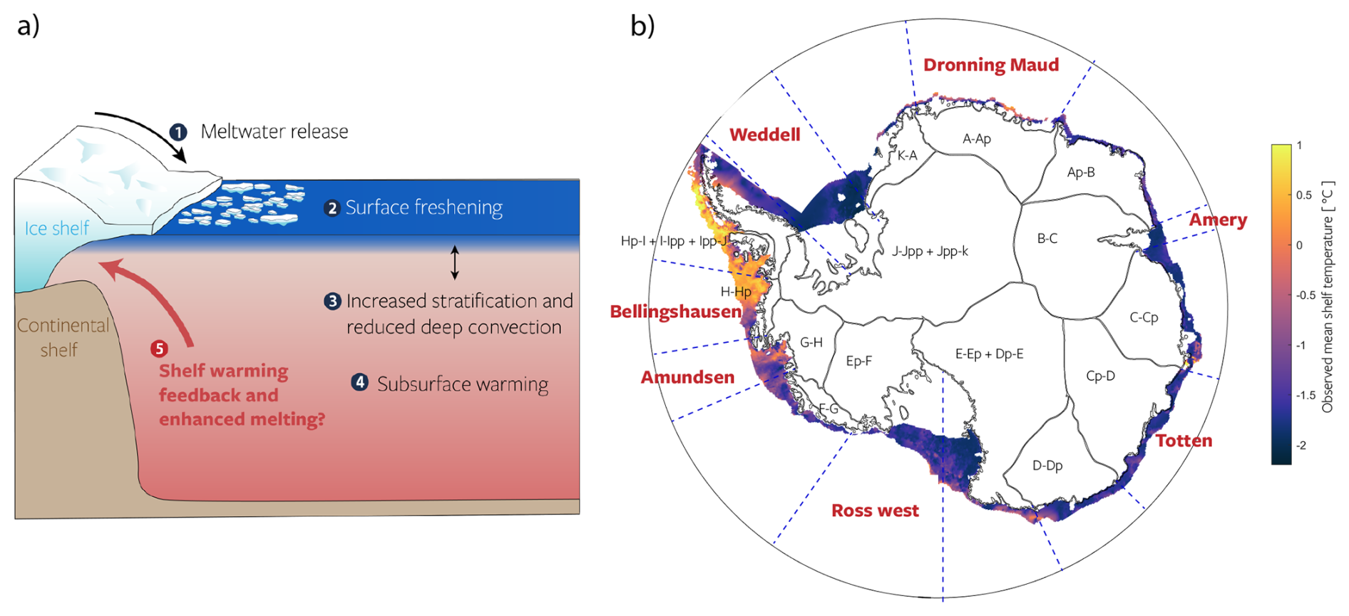
Figure 1 (a) Schematic illustrating the impact of Antarctic Ice Sheet meltwater on Southern Ocean hydrography, emphasizing the potential subsurface ocean warming and ice shelf melting feedback mechanisms explored in this study. (b) Antarctic Ocean sectors (blue dashed lines) used in this study, based on definitions by Jourdain et al. (2020), originally derived from Mouginot et al. (2017) and Rignot et al. (2019). Individual drainage basins (black contours) are shown but are not utilized here. For this study, the following original sectors have been combined: E–Ep + Dp–E, J–Jpp + Jpp–k, and all sectors on the Antarctic Peninsula. Color shadings indicate depth-average (surface-bottom) temperatures (°C) along the Antarctic shelf (poleward of the 1000 m isobath until the ice shelf front) from observations (Sect. 2.3; Zhou et al., 2026).

This problem is not new; over the past few decades, numerous studies have explored this topic on various spatial and temporal scales. A comprehensive list of these studies is provided in Swart et al. (2023). These studies typically rely on freshwater perturbation experiments, often referred to as “hosing experiments”, where the ocean is forced with additional freshwater using coupled climate models or ocean–sea-ice-only simulations. A key limitation of these studies is the lack of consistency in the experimental design. Approaches vary widely in the magnitude, spatial and temporal distribution of freshwater forcing, and the methods used to impose freshwater and heat fluxes associated with ice melt. Most models do not include ice shelves and icebergs, representing meltwater as runoff from the continent and simulating its entry into the ocean at the surface rather than at depth. Moreover, most Southern Ocean hosing experiments have been conducted using single models, ranging from simple theoretical frameworks and simplified intermediate-complexity models, to fully-coupled Earth System Models with varying but generally coarse spatial resolutions. As a result, the findings across these existing studies are highly model-dependent, often yielding divergent or even contradictory conclusions regarding responses on the continental shelf. Additionally, the diversity in experimental designs, including the background climate ranging from preindustrial to various global warming scenarios, and freshwater forcing styles not only complicates direct comparisons between studies but also hinders the assessment of model spread, which is typically achieved through coordinated intermodel comparison projects, e.g., the CMIP framework (Eyring et al., 2016).

Despite variations across previous studies, certain responses to additional meltwater appear qualitatively robust. Offshore from the continental break, the Southern Ocean water column is characterized by a cold surface layer overlying a warmer deep layer known as Circumpolar Deep Water (CDW). Models consistently show that additional freshwater reduces surface water density, strengthening water column stratification and isolating the (relatively) warm CDW from the surface where atmospheric cooling occurs. This creates cold near-surface temperature anomalies and warm anomalies at depth, (Fig. 1a). The effects of this redistribution of heat from freshwater “capping” includes the cooling of Southern Hemisphere sea surface and air temperatures (Stouffer et al., 2007; Beadling et al., 2024; Xu et al., 2025; Kaufman et al., 2025), the expansion of Antarctic sea ice (Beckmann and Goosse, 2003; Hellmer, 2004; Pauling et al., 2016, 2017; Merino et al., 2018; Purich et al., 2018), the reduction of Antarctic Bottom Water (AABW) formation (Fogwill et al., 2015; Lago and England, 2019; Mackie et al., 2020a; Li et al., 2023; Tesdal et al., 2023; Chen et al., 2023), and the warming of the deep ocean (Hansen et al., 2016; Bronselaer et al., 2018; Jeong et al., 2020; Haumann et al., 2020; Moorman et al., 2020; Beadling et al., 2022).

A key question is how these offshore changes interact with the different continental shelf regimes around Antarctica (Thompson et al., 2018), e.g., to what extent stratification-induced deep-ocean warming anomalies propagate to the coast (Thomas et al., 2023), where positive and negative feedbacks have been proposed in response to meltwater input (Bronselaer et al., 2018; Golledge et al., 2019; Snow et al., 2016; Hattermann and Levermann, 2010; Swingedouw et al., 2008).

Using a high-resolution ocean model, Moorman et al. (2020) showed that coastal freshening can both strengthen density gradients along the Antarctic Slope Front – reducing exchange between cold shelf waters and warmer offshore waters (Hellmer et al., 2017; Hattermann, 2018; Si et al., 2023) – and intensify the westward ASC and ACoC, enhancing lateral connectivity between shelf regions (Dawson et al., 2023). A stronger ASC and ACoC can transport colder waters from the western Weddell Sea into the warmer Bellingshausen and Amundsen Seas, driving cooling in West Antarctica (Beadling et al., 2022; Moorman et al., 2020). This westward advection of colder waters does not necessarily result only from strengthened currents; it can also result from a reduction in the formation of Dense Shelf Water (DSW) from the Weddell Sea. Coastal freshening produces slightly lower density DSW that is injected mid-depth rather than sinking and flowing offshore, causing these lighter waters to become entrained in coastal and slope currents and advected westward around the Antarctic Peninsula (Morrison et al., 2023a). Similar connective links between continental shelf sectors extend along the entire Antarctic margin (Dawson et al., 2023; Beadling, 2023); for example, upstream meltwater advection may also contribute to additional shelf warming in the southern Weddell Sea (Hoffman et al., 2024).

Capturing these processes and shelf connectivity depend on the model's ability to represent continental shelf and slope dynamics that govern heat transport between the shelf and the open ocean, such as localized dense shelf water overflows (Daae et al., 2020; Morrison and et al., 2020), interaction between the ASC and troughs at the continental shelf break (Gómez-Valdivia et al., 2023), episodic atmospheric wind forcing (Morrison et al., 2023b; Dundas et al., 2024), and eddy-driven shoreward transport of CDW (Stewart et al., 2018). Representation of these processes is resolution dependent as the Rossby radius of deformation approaches 1–2 km near the continental shelf (Hallberg, 2013) and a minimum nominal horizontal resolution of 50 km has been shown to be required to resolve robust westward flow along the slope (Mathiot et al., 2011). For example, Beadling et al. (2022) imposed a 0.1 Sv meltwater perturbation in two models with different ocean resolutions (GFDL-CM4 at 0.25° and GFDL-ESM4 at 0.5°) and found markedly different responses: the finer‐resolution GFDL-CM4 simulated a stronger ASC that insulated the West Antarctic shelf from offshore warming, whereas the coarser GFDL-ESM4 allowed meltwater to disperse offshore, leading to shelf warming. However, to what extent the interplay of stratification-induced warming, cross-shelf isolation, and along-shelf homogenization influences the response to meltwater input in other CMIP-style models remains unknown.

In addition to uncertainties in open ocean–shelf interactions, there is considerable regional and temporal variability and uncertainty about how continental shelf temperature anomalies influence basal melting. Ice shelf basal melting is primarily governed by the ocean properties beneath the ice and the turbulent processes that transport heat to the ice-ocean interface (Holland and Jenkins, 1999; Rosevear et al., 2025). Since most CMIP-style models do not include ice shelf cavities, basal melt rates in ice sheet models forced by climate models are typically derived using parameterizations that relate melting to ocean thermal forcing extrapolated from “far field” ocean conditions on the continental shelf (Jourdain et al., 2020). Thermal forcing is defined as the difference between the in situ temperature of the ocean and the melting temperature of the ice at the pressure of the ice shelf base. These parameterizations typically try to account for the modification of ocean properties by the buoyant melt plume along the ice shelf base and subsequent buoyancy-driven circulation in cavities (Jenkins, 1991; Burgard et al., 2022). Parameterizations commonly follow a quadratic function of thermal forcing (Holland, 2008), and approaches such as regional calibrations (Jourdain et al., 2020) and linear response function frameworks (Lambert et al., 2025) have been proposed to account for regional variations in the observed Antarctic melt rates. However, a significant challenge lies in the scarcity of observational data on oceanographic conditions needed to calibrate these parameterizations. Although basal melt rates can be estimated from remote sensing products (Rignot et al., 2019; Adusumilli et al., 2020; Paolo et al., 2023), direct measurements near or below the ice shelves remain exceedingly rare. As a result, basal melting parameterizations remain poorly constrained, contributing significant uncertainty to estimates of future ice shelf mass loss.

Another key challenge in assessing potential feedback mechanisms is separating the effects of meltwater forcing from broader changes induced by global warming. Some global warming trends, such as deep ocean warming (Purich and England, 2021), can produce spatial and temporal patterns similar to those driven by increasing meltwater input, making it difficult to isolate individual contributions. Furthermore, global warming alters the hydrological cycle and reduces brine rejection on the continental shelf as sea ice formation reduces, introducing additional freshwater sources that can have impacts similar to those of Antarctic meltwater discharge (Lockwood et al., 2021). For example, Goddard et al. (2017), Ong et al. (2025), and Dawson et al. (2025) found ASC responses similar to those reported by Moorman et al. (2020) in response to shelf freshening induced by global warming without additional meltwater forcing. Observational evidence suggests that some of these changes could already be playing out as warming trends in the deep Southern Ocean (Jacobs and Giulivi, 2010; Bintanja et al., 2013; Johnson and Purkey, 2024) suggest potential changes to AABW formation and export processes emanating from Antarctic shelf dynamics. However, it is unclear to what extent the observed trends in bottom water properties are influenced or driven by on-going changes in meltwater discharge versus other changes in the Southern Ocean freshwater cycle or general warming trends. Earlier simulations that incorporate meltwater forcing based on current Antarctic discharge estimates, combined with high greenhouse gas emission scenarios (RCP8.5), project deep ocean temperature increases between 1 and 2 °C (Bronselaer et al., 2018; Sadai et al., 2020). However, it remains uncertain to what extent these warming patterns are modified by processes identified in standalone meltwater experiments. Specifically, whether climate warming or meltwater input exerts a greater influence on continental shelf properties, or whether meltwater discharge amplifies or counteracts broader global warming-induced changes, also remains an open question (Mackie et al., 2020b).

All of the challenges discussed above are compounded by substantial biases in the ocean properties simulated by climate models. Climate models contributed to CMIP have been shown to exhibit significant variability in their representation of the water masses of the Southern Ocean (Sallée et al., 2013; Heuzé et al., 2013; Beadling et al., 2019, 2020; Heuzé, 2021), making it difficult to assess whether they realistically capture the conditions necessary to generate accurate ice sheet forcing (Barthel et al., 2020). To mitigate the influence of large mean-state biases, Jourdain et al. (2020) proposes using only anomalies relative to the modern era for ice shelf forcing. However, this approach does not fully resolve the issue, as biases in the mean state may still influence projected anomalies. The extent to which model responses depend on their mean state has yet to be fully quantified.

In summary, uncertainties in simulating ice shelf basal melting arise from multiple factors:

• a.

  model- and scenario-dependent climate response and feedback to meltwater discharge

• b.

  the complex interactions between the open ocean and the continental shelf

• c.

  the parameterization of basal melting, which remains poorly constrained due to limited observations

• d.

  the combined influence of meltwater and broader global warming-induced changes

• e.

  biases in climate models' representation of Southern Ocean water mass properties and incomplete representation of near-shelf dynamics

In this study, our objective is to assess all these contributing factors. To address (a), we use a unique set of experiments from a suite of climate models that contributed simulations to the Southern Ocean Freshwater Input from Antarctica (SOFIA) initiative (Swart et al., 2023). SOFIA provides an experimental framework and coordinated effort that is specifically designed to constrain the climate impacts of additional meltwater associated with Antarctic mass loss and quantify uncertainties from its exclusion in projections. Although similar in spirit to previous hosing experiments, the strength of SOFIA lies in its strict protocol on freshwater timing, magnitude, and distribution, ensuring consistency across models with differing horizontal and vertical resolution, vertical coordinates, subgrid-scale parameterizations, numerics, and mean-state biases.

Our work builds on Chen et al. (2023), who examined the Southern Ocean deep convection response to Antarctic meltwater in a subset of the SOFIA models. We additionally address (b) by assessing whether offshore reductions in deep convection induce continental shelf warming and by analyzing the spatial variability of this response.

To address (c), we update and calibrate a regional basal melting parameterization, assessing whether shelf warming amplifies ice shelf melting and accelerates Antarctic mass loss.

Furthermore, to address (d), we compare the ocean response to meltwater with the broader changes induced by global warming in SSP5-8.5 scenario simulations to examine whether meltwater is likely to reinforce or counteract warming-driven trends.

Finally, to address (e), we assess the relationship between model response and mean-state biases by incorporating a new high-resolution observational hydrographic climatology. This climatology also aids in refining the basal melting parameterization, providing new insights into the future of Antarctic mass loss.

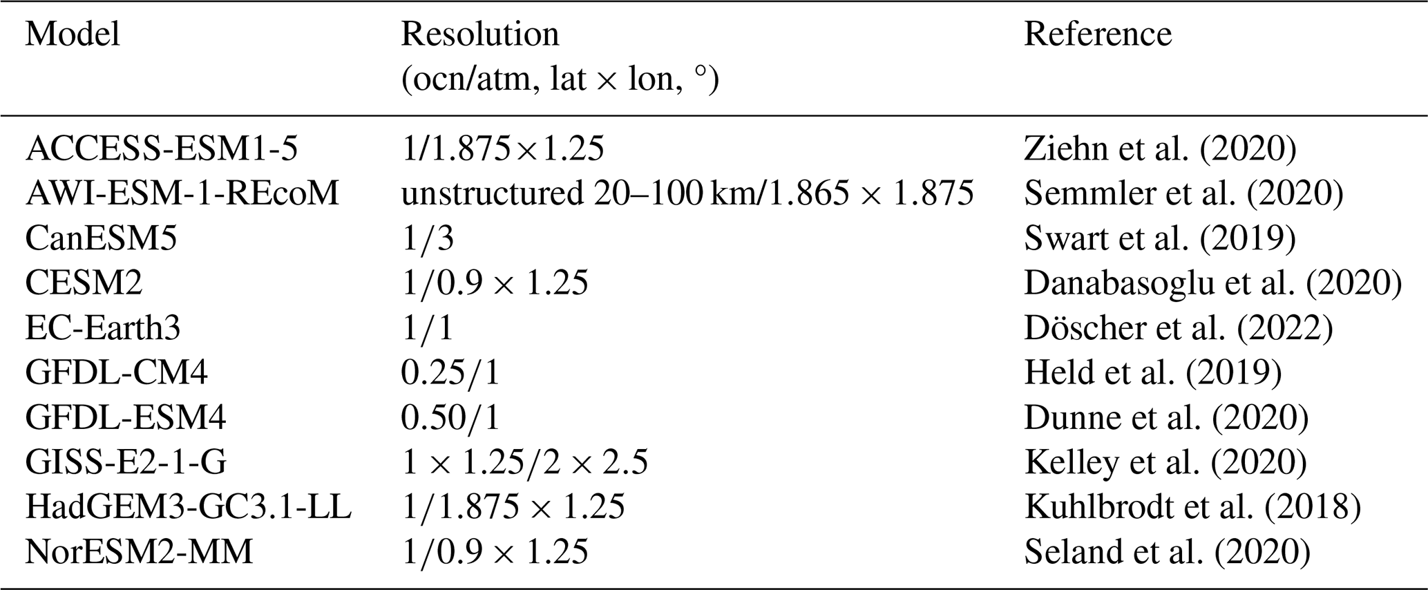
Ziehn et al. (2020)Semmler et al. (2020)Swart et al. (2019)Danabasoglu et al. (2020)Döscher et al. (2022)Held et al. (2019)Dunne et al. (2020)Kelley et al. (2020)Kuhlbrodt et al. (2018)Seland et al. (2020)

Table 1 List of models participating in the SOFIA Tier 1 antwater experiment used in this analysis. Throughout the manuscript we refer to ACCESS-ESM1-5 as ACCESS-ESM1, AWI-ESM-1-REcoM as AWI-ESM, GISS-E2-1-G as GISS-E2, HadGEM3-GC3.1-LL as HadGEM3 and NorESM2-MM as NorESM2.

2 Methods

2.1 Models and Experimental Design

We use monthly-mean model output obtained from 10 CMIP6 models (Table 1) participating in the antwater (Tier 1) experiment described in the SOFIA experimental design (Swart et al., 2023). The models used in this study are the same as those employed in a parallel study (Pauling et al., 2026), which evaluates the response to sea ice. Following the SOFIA protocol, the antwater experiments are branched from the (spun-up) model's piControl run. While all other external forcings are kept under the piControl conditions, a constant flux of 0.1 Sv (3154 Gt yr⁻¹) of additional meltwater is evenly distributed at the surface across all grid cells adjacent to the Antarctic coast. We note that this amount of meltwater is significantly larger than current observational estimates of basal melt rates on the ice shelf (Adusumilli et al., 2020; Paolo et al., 2023) or Antarctica's current mass imbalance (Slater et al., 2021; Otosaka et al., 2023). However, the antwater experiment is designed to generate a robust signal for model intercomparison, rather than to replicate observed melt rates, and it is not an excessive amount in terms of end-of-21st-century projections (IPCC, 2019). The models employ different vertical and horizontal resolution, but all implemented extra meltwater at the surface at each model time step. The antwater experiment runs for 100 years, and most of the results in our study are presented as anomalies that compare the time averages of the last 10 years antwater run against the corresponding time period of the CMIP6 piControl run.

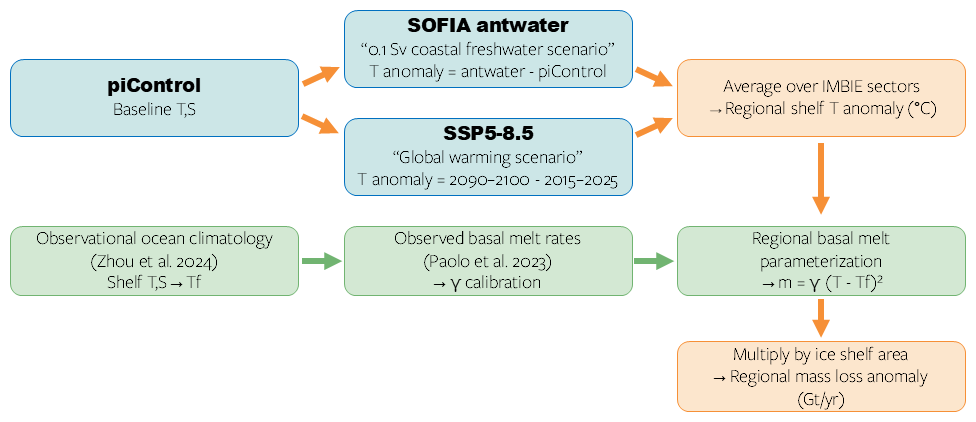
Figure 2 Overview of the simulations analyzed in this study and the methodology used to calculate total ice shelf mass loss anomalies based on ocean temperature anomalies.

SOFIA Tier 2 scenario experiments (Swart et al., 2023) are designed to assess the combined effects of added Antarctic meltwater forcing under future climate conditions. As these simulations are not yet available, we instead compare the antwater experiments with future scenario SSP5-8.5 (Meinshausen et al., 2020) anomalies from the CMIP6 ScenarioMIP simulations (O'Neill et al., 2016) from the same models to evaluate meltwater effects relative to broader global warming–induced trends. The SSP5-8.5 anomalies represent the change by the end of the 21st century, computed as difference between years 2090–2100 and years 2015–2025. An overview of the different simulations is presented in Fig. 2. For each model, only a single run was used, as not all models provided an ensemble. All computations were performed on the models' native grids, except AWI-ESM, whose native grid is unstructured. We calculate model bias as the difference between the model's piControl state (last 10 years) and an observationally-based climatology (Sect. 2.3), with the climatology regridded to match the respective model grids. Here, we use the term bias in a broad sense, as we are comparing preindustrial piControl conditions – nominally representing the year 1850 – with modern-day observations. While this is not a strict like-for-like comparison, the intent is not to assess the models' skill for a specific historical period. Rather, it is to illustrate the overall offset between the simulated piControl state and the observed climate system. We deliberately do not compare with historical simulations, as our aim is to evaluate the model state at the branching point of the antwater experiments. The model output used in this study include ocean potential temperature (“thetao”), salinity (“so”), eastward and northward ocean velocity (“uo” and “vo”), and the age of seawater since surface contact (“agessc”).

Although SSP5-8.5 simulations lack fully interactive ice sheets, they still include additional freshwater inputs from changes in the hydrological cycle, such as altered precipitation, evaporation, continental runoff, and sea ice processes. Models show that precipitation-evaporation (P−E) patterns have already changed (Purich et al., 2018) and are projected to change significantly in the future (Held and Soden, 2006; Bracegirdle et al., 2020; Seroussi et al., 2024). Furthermore, models without an interactive ice sheet likely reroute precipitation over the Antarctic continent directly into the ocean as runoff and/or calving. Seasonally and regionally averaged, sea ice growth and melt have a limited impact on the Southern Ocean's net freshwater budget, as most ice grows and melts locally. However, brine rejection remains an important process on the continental shelf (Dawson et al., 2025). To effectively compare the SSP5-8.5 simulations with the antwater experiments, it is thus essential to assess the changes in various surface freshwater sources and determine how they compare with the 0.1 Sv anomaly in antwater. Figure 3a shows the SSP5-8.5 end-of-the-century anomalies in total freshwater input (“wfo”), evaporation (“evs”), precipitation (“prra”), and river runoff (“friver”) integrated over the entire Southern Ocean south of 60° S. “wfo” includes fluxes associated with calving and sea ice growth and melt, but these are not included in the decomposition as they were not available for most models. Additionally, a small mismatch between the decomposed terms and the total “wfo” may arise because E-P represent fluxes over the entire grid cell and therefore include precipitation falling on sea ice and evaporation/sublimation from sea ice that do not directly enter the ocean but modify the sea ice/snow mass and ultimately the flux associated with melt and growth. Furthermore, potential flux-correction terms and the advection of sea ice are not accounted for in the decomposition.

The total freshwater anomaly in the SSP5-8.5 simulations is relatively consistent between models, with a multi-model mean of 0.14 Sv – slightly higher than the 0.1 Sv added in antwater. However, we note that, unlike the constant step forcing in antwater, this anomaly evolves over time and is seasonally dependent. In SSP5-8.5, additional surface freshwater is primarily driven by changes in precipitation minus evaporation (P−E; blue bars in Fig. 3a), with a smaller contribution from continental runoff (<20 % of the anomaly). The resulting surface salinity changes, spatially averaged over the Southern Ocean, range from −0.15 to −0.55 psu in SSP5-8.5, comparable to the salinity change in antwater. We note, however, that the horizontal distribution of the freshwater is very different. In most models, freshwater from runoff and calving is spread out over a much larger area, whereas in antwater the freshwater is added adjacent to the coast (see Fig. 1 in Kaufman et al., 2025). The purpose of this analysis is to clarify how to interpret the comparison between SSP5-8.5 and antwater anomalies. While antwater anomalies represent the isolated effect of meltwater alone, SSP5-8.5 anomalies reflect a combination of global warming-induced changes, including stratification changes due to freshwater anomalies of similar magnitude to antwater. However, since SSP5-8.5 does not include additional meltwater forcing, the changes induced by antwater could be considered additive to the broader effects observed in SSP5-8.5. Of course, this assumes a linear relationship, which is not entirely accurate (Sect. 4.2 and 4.4).

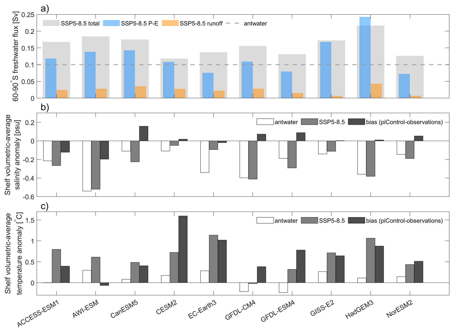
Figure 3 (a) Magnitude of total freshwater input (Sv) anomaly (shoreward of 60° S) under SSP5-8.5, decomposed into contributions from runoff and precipitation-evaporation (P−E), compared to the 0.1 Sv in the antwater experiment. The residual of this decomposition includes contributions from sea ice melt/freeze and iceberg calving, which are not available consistently across all models but are part of the total freshwater anomaly shown by the grey bars. Fluxes related to sea ice melt and freeze are important for seasonal freshwater redistribution but are of limited relevance in annual means and are therefore examined in detail by Pauling et al. (2026). (b) Volumetric-average salinity change and bias on the continental shelf (surface-bottom, poleward of the 1000 m isobath until the ice shelf front) in the meltwater perturbation experiments (antwater – piControl) and under SSP5-8.5 (comparing 2090–2100 with 2015–2025). (c) Same as (b) but for temperature.

2.2 Model Output Analysis

Following Jourdain et al. (2020), we assess both offshore deep ocean properties and continental shelf water masses, which are critical for ice shelf–ocean interactions. This approach contrasts with studies that rely on large-scale latitudinal averages (e.g., Levermann et al., 2020; Lambert et al., 2025). To systematically investigate spatial variability, we analyze different sectors around Antarctica (Fig. 1b), which, for consistency with the Ice Sheet Model Intercomparison Project (ISMIP6; Seroussi et al., 2020), follow the sector definitions of Jourdain et al. (2020). These sectors are based on the latest Ice Sheet Mass Balance Inter-comparison Exercise (IMBIE) assessment (IMBIE, 2018; Otosaka et al., 2023) and are delineated using drainage basin boundaries derived from satellite-observed ice sheet surface elevation and velocity data (Mouginot et al., 2017; Rignot et al., 2019). To ensure alignment with coarse model grids and observational data while avoiding the division of similar oceanic “basins”, we combine the following sectors: E–Ep + Dp–E, J–Jpp + Jpp–k, and all sectors on the Antarctic Peninsula. Our oceanic sectors are defined by the longitudinal boundaries of the drainage basins, which extend into the open ocean until they reach the continental shelf break. The boundary between the shelf and the open ocean is marked by the 1000 m isobath, except in the large embayments of the Ross and Weddell seas, where the offshore boundaries follow the definitions of Barthel et al. (2020), which use a combination of bathymetry shallower than 1000 m and fixed northern boundary at 74° S. We adhere to the IMBIE naming convention but focus specifically on seven key sectors, referred to here by their more commonly recognized names: Weddell, Dronning Maud Land, Amery, Totten, Ross West, Amundsen, and Bellingshausen (Fig. 1b).

Consistent with Barthel et al. (2020), who evaluated the output of the CMIP5 models for ice sheet forcing, the oceanic properties on the continental shelf are calculated as full-depth volume averages (from the surface to the bottom, down to 1000 m depth or less) poleward of the continental shelf break and extending to the “coast”. These boundaries vary between models depending on their resolution and bathymetry. By using the broadest definition (full water column), we reduce the influence of biases in the vertical distribution of water masses found in some models, and maintain consistency with previous studies. While we acknowledge that temperature responses on the shelf are not vertically uniform, the impact on final results is minor: for example, excluding or including the surface layer alters regional multi-model median temperature anomalies (Sect. 3.2) by only 0.001 to 0.028 °C, corresponding to relative changes below 7 %, with a median absolute difference of just 0.015 °C.

2.3 Contemporary Ocean Climatology

A key limitation in assessing ocean ice shelf interactions is the availability of accurate observational datasets, as many global ocean climatologies exhibit biases in coastal regions around Antarctica. In this study, we used a new regional ocean climatology derived from historical CTD, Argo, and seal-borne profiler data (Zhou et al., 2024), providing a more refined representation of Antarctic coastal ocean properties. The reader is referred to Zhou et al. (2026) for full details of the method used to generate the climatology. Here, we briefly introduce the assumption adopted in the creation of ocean climatology.

Assuming anisotropy in water mass properties along ocean currents, the climatology assembles and averages all temperature and salinity profiles within along-flow elongated ellipses. In turn, mean ocean flow is determined using sea surface height (SSH) contours, a proxy for the barotropic geostrophic component of ocean circulation. SSH is provided by the 139th iteration of the Southern Ocean State Estimate (SOSE, Mazloff et al., 2010), which assimilates observations of not only temperature/salinity profiles but also moored time series and surface measurements such as the height of the open ocean sea surface, temperature, salinity and sea ice concentration. The SSH field, therefore, covers the sea-ice area and provides a dynamically conserved estimation of the ocean circulation.

2.4 Basal Melting Parameterization

To evaluate the impact of meltwater‐induced and global‐warming‐induced changes, we use a simplified basal melt parameterization to convert simulated coastal ocean temperature anomalies into basal mass loss anomalies. Our approach follows the quadratic relationship between basal melt rates and thermal forcing proposed by Holland (2008) and widely applied in ice sheet modeling studies (Beckmann and Goosse, 2003; Favier et al., 2019; Jourdain et al., 2020). In this framework, basal melt depends on the difference between in situ ocean temperature and the local freezing point at the ice shelf base, scaled by an effective exchange velocity that captures the efficiency of heat transfer within the cavity. Previous work has shown that this efficiency varies regionally depending on ice shelf geometry and associated melt‐driven circulation (Jenkins, 1991; Little et al., 2009; Jourdain et al., 2020), motivating regionally calibrated melt coefficients.

2.4.1 Regional melt coefficient calibration

For each region j, we compute a local melt rate coefficient γ_j using observed ocean conditions (Sect. 2.3) and satellite‐derived basal melt rates (datasets described in Sect. 2.5). We first extract the climatological thermal forcing,

$$\begin{array}{}\text{(1)}& T_j^{\mathrm{obs}}-T_{\mathrm{f}}^{\mathrm{obs}},\end{array}$$

where $T_j^{\mathrm{obs}}$ is the observed volume‐averaged temperature on the continental shelf (south of the 1000 m isobath), and $T_{\mathrm{f}}^{\mathrm{obs}}$ is the in situ freezing temperature at the regional mean ice shelf draft, based on climatological salinity. The regional melt coefficient is then obtained following Jourdain et al. (2020):

$$\begin{array}{}\text{(2)}& {\mathit{\gamma }}_j={\displaystyle \frac{{\dot{m}}_j^{\mathrm{obs}}}{(T_j^{\mathrm{obs}}-T_{\mathrm{f}}^{\mathrm{obs}}{)}^{\mathrm{2}}}}\end{array}$$

2.4.2 Basal melt rate estimation

Once γ_j is determined, the basal melt rate ${\dot{m}}_j$ corresponding to simulated ocean conditions is calculated as:

$$\begin{array}{}\text{(3)}& {\dot{m}}_j={\mathit{\gamma }}_j{\left(T_j-T_{\mathrm{f}}\right)}^{\mathrm{2}},\end{array}$$

where T_j is the simulated shelf temperature anomaly averaged over region j, and T_f is the corresponding in situ freezing temperature at the ice shelf base. This formulation allows us to translate simulated thermal forcing anomalies into regional basal melt anomalies consistent with observed present‐day melt regimes.

2.5 Observed Melt Rates and Ice Shelf Draft

Our basal melting parameterization relies on the updated satellite-derived dataset of Antarctic ice shelf basal melt rates from Paolo et al. (2023), which provides a 26-year (1992–2017) pan-Antarctic time series of ice shelf thickness and melt rates at 3 km resolution using four radar altimeters. This dataset offers both longer temporal coverage and finer spatial resolution than previous Antarctica-wide estimates (Depoorter et al., 2013; Rignot et al., 2013; Adusumilli et al., 2020). For our application, we compute area-weighted mean melt rates for each sector over the full observation period. To determine the temperature difference relative to the in situ freezing point at the ice shelf base, we use the high-resolution ice shelf draft dataset developed by Moholdt and Maton (2024), averaged over the same sectors shown in Fig. 1b.

3 Results

3.1 Regionally Varying Meltwater-induced Subsurface Warming

As previously shown by Chen et al. (2023), the zonal mean temperature anomaly across the different models reveals distinct patterns of warming and cooling in the Southern Ocean in response to the antwater meltwater perturbations (Fig. 4). All models consistently show a cooling response at the surface and warming in the deeper ocean layers, which aligns with the expected stratification-induced effects of meltwater. For some models, the warming anomaly extends to the surface near the continent, but for most models, the maximum anomaly is below 1500 m. In general, the response is strongest around and south of 65° S latitude, corresponding to key regions of modeled (impeded) deep water formation (Heuzé, 2021, show that CMIP6 models typically fail to produce dense water in the same regions where it forms in the real world). There is a wide range of warming magnitudes, where models such as AWI-ESM, GFDL-CM4 and GISS-E2 exhibit pronounced warming (>1 °C), while others such as ACCESS-ESM1 and NorESM2 show relatively subdued warming. No clear relationship between model resolution and the simulated response is evident (all models are considered “coarse” (≈1°) except GFDL-CM4, GFDL-ESM4 and AWI-ESM). Above the subsurface warming, models consistently exhibit surface cooling (consistent with results from Kaufman et al., 2025), though its intensity and vertical extent vary across models. This cooling anomaly promotes the expansion of sea ice, as shown in a parallel study (Pauling et al., 2026), which also links the extent of surface cooling to mean-state stratification – consistent with our finding that models exhibiting strong surface cooling tend to show pronounced warming at depth.

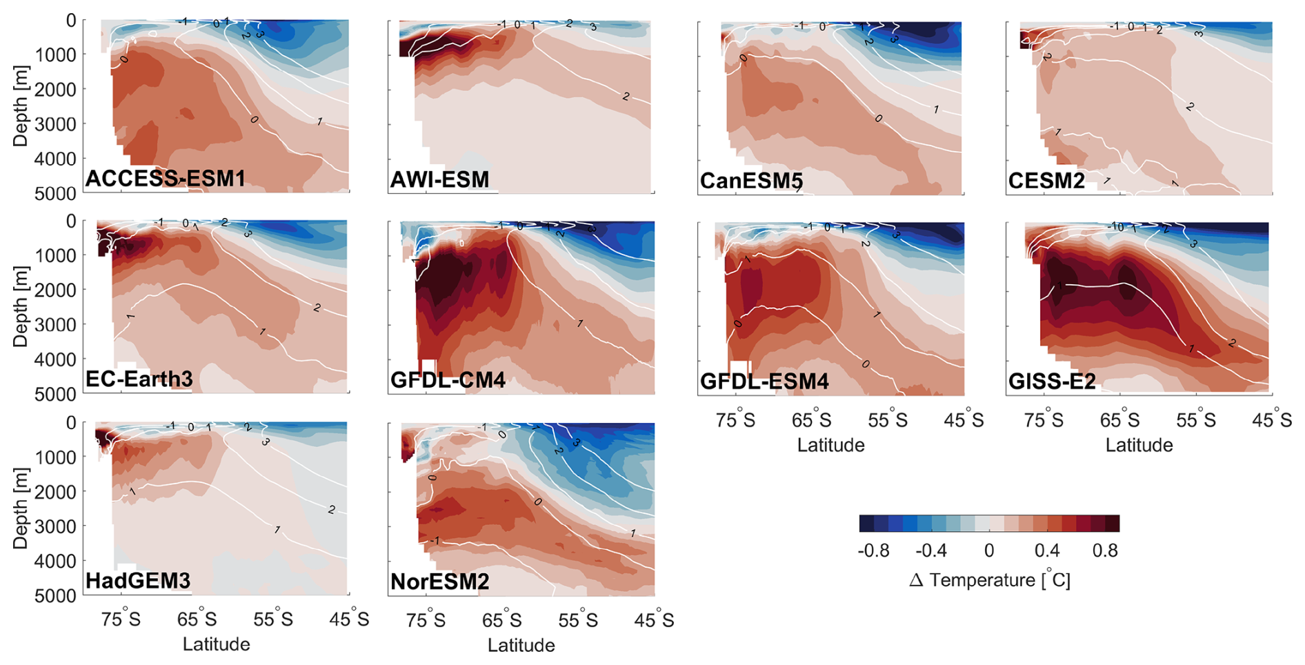
Figure 4 Zonal mean temperature change in response to meltwater perturbation (°C; antwater – piControl; last 10 years) for all models. White contours represent the climatological mean temperature in piControl.

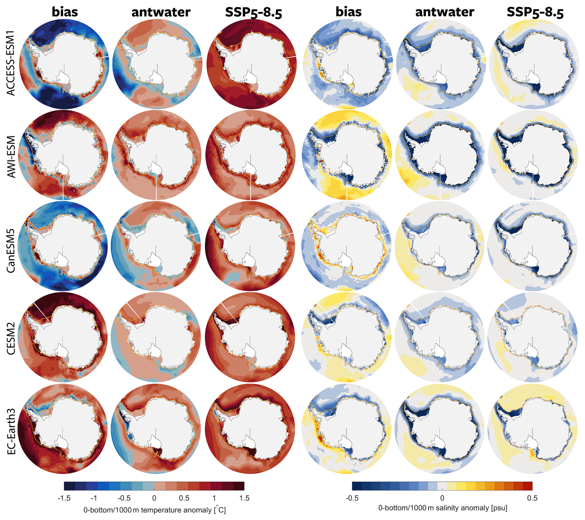
Figure 5 Spatial maps of surface–1000 m/bottom depth-averaged model temperature (°C) and salinity. The first column shows temperature bias (piControl–observations), the second column shows temperature change due to meltwater perturbation (antwater–piControl, comparing the last 10 years), and the third column shows temperature change under SSP5-8.5 (comparing 2090–2100 with 2015–2025). Columns 4–6 display the corresponding salinity maps. The 1000 m isobath, marking the boundary between the continental shelf and the open ocean, is contoured in each panel.

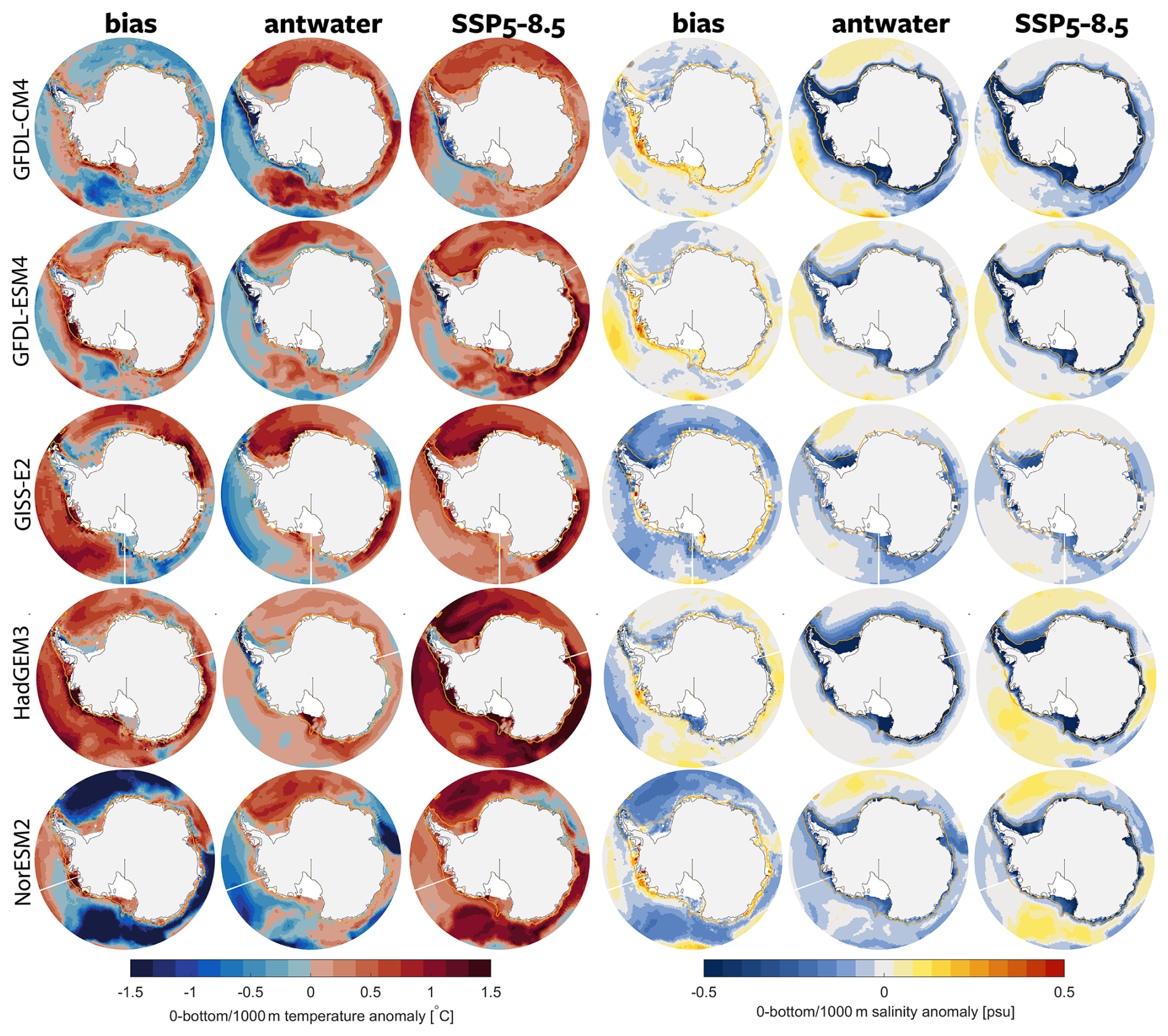
Figure 6 Continuation of the spatial anomaly maps shown in Fig. 5.

At the continental shelf break and on the continental shelf, there are pronounced inter-model differences in both the sign and magnitude of the temperature anomalies resulting from the antwater experiment. The zonal mean, volume-averaged temperature anomaly over the continental shelf (from surface to bottom, poleward of the 1000 m isobath) is generally positive across most models (as also shown in Fig. 3c), but notably negative in both GFDL models, discussed further below.

Although the zonal mean provides a broad overview of the temperature response to meltwater, previous studies (Beadling et al., 2022) have shown strong regional variations, and thus a zonal mean is less appropriate to study changes along the continental shelf, requiring us to examine how these responses differ between key sectors. Figures 5 and 6 present the spatial distribution of antwater anomalies in relation to model biases and the temperature anomalies projected under the SSP5-8.5 global warming scenario. In particular, the temperature biases in most models (first column in Figs. 5 and 6; piControl minus observations) are larger than the anomalies induced by the antwater experiment (second column). The biases exceed 1 °C in both positive and negative directions, displaying pronounced differences among models. It is important to note, however, that some degree of cool bias is expected, since the piControl simulations represent pre-industrial conditions, while the observations reflect a climate that has already experienced over a century of global warming. Consequently, warm biases in the models suggest they may be substantially too warm. Some models, such as CESM2, EC-Earth3, GISS-E2, and HadGEM3, show predominantly warm biases across all regions surrounding the Antarctic continent. In contrast, ACCESS-ESM1 and NorESM2 are predominantly biased cold, except in regions like West Antarctica and the Totten and Amery sectors. CanESM5 and both GFDL models show a distinct pattern of warm biases along the coast, transitioning to cold biases farther offshore.

Temperature biases are especially large on the continental shelf. Near the coast, most models exhibit warm biases, particularly in West Antarctica, with AWI-ESM being the only model that shows cold biases in this region. Salinity biases also tend to be large near the coast (fourth column in Figs. 5 and 6). Although most models exhibit a fresh bias across the open Southern Ocean (a well-known bias in CMIP6 models, Purich and England, 2021, shared with the CMIP5 predecessors; Beadling et al., 2019), coastal regions, particularly in West Antarctica, tend to be too saline, pointing to a bias in the properties, residence time or amount of CDW on the shelf. An exception of the too saline shelves is the southern Weddell Sea, where most models show a fresh bias even on the shelf, likely due to the absence of wind-driven coastal polynyas that facilitate the formation of sea ice and the densification of the shelf water masses (Vernet et al., 2019). Model resolution is likely a key factor; for example, the relatively high-resolution GFDL models form dense shelf water in the Weddell Sea via coastal polynyas in their mean state (Tesdal et al., 2023) and exhibit smaller salinity biases in this region.

Large biases on the continental shelf are expected, as these regions are difficult to resolve and require capturing cross-front exchanges and coastal water-mass transformation processes that depend on mesoscale eddies (Hallberg, 2013). Additionally, the observation based climatology also carries greater uncertainty on the continental shelf (Zhou et al., 2026) and may be affected by undersampling of internal variability.

Spatial patterns in response to the antwater meltwater simulations are remarkably consistent in all models, showing greater agreement than mean-state biases. Generally, a meltwater perturbation induces an offshore warming anomaly in the upper 1000 m, but this warming is not uniform across all regions. Figures 5 and 6 illustrate that the offshore circumpolar mean warming shown in Fig. 4 is primarily driven by warming in the Weddell Sea and along the east Antarctic coast, while an offshore cooling anomaly is evident in most models west of the Antarctic Peninsula. These patterns underscore substantial regional differences, demonstrating that a zonal mean alone is insufficient to represent changes in the Southern Ocean. As expected, the SSP5-8.5 simulations show a widespread warming in all models (third column in Figs. 5 and 6). Some regional differences also appear in the SSP5-8.5 simulations, though they are much weaker than in the antwater experiments, and only the GFDL models show any indication of cooling near the Antarctic Peninsula. This asymmetric response and the potential mechanisms driving the cooling will be addressed in detail in Sects. 3.2 and 4.3. It is also important to note that, even when averaging over multiple years, natural variability may still contribute to some of the spatial differences seen in the anomaly maps (Purich and England, 2021), as many of these models exhibit substantial multi-decadal and centennial-scale variability (see Supplement in Beadling et al., 2020).

In the antwater simulations, the models vary significantly in whether the warm offshore anomalies in the Weddell Sea and East Antarctica extend southward past the continental shelf break. In some models, the warming response is equally strong near the coast as offshore, while in others, the magnitude of coastal anomalies is somewhat reduced. In the SSP5-8.5 simulations, the most pronounced temperature increases occur in the open ocean, whereas coastal regions, particularly near the shelf break, exhibit more moderate warming. The Amundsen and Bellingshausen regions are exceptions, showing little or no gradient across the shelf break in both antwater and SSP5-8.5, consistent with the direct isopycnal connection characteristic of this “warm” shelf regime (Thompson et al., 2018). Although the spatial patterns of SSP5-8.5 anomalies are relatively consistent across models, there is considerable variation in magnitude.

Similar to the temperature response, models exhibit substantial variation in the northward extent of negative salinity anomalies: in some cases, freshening is confined to the immediate coastal zone, while in others it extends farther offshore. GFDL-CM4 and AWI-ESM show the strongest salinity response near the coast (see also Fig. 3b). Interestingly, these are the models with the highest spatial resolution along the coast. This is consistent with the findings of Beadling et al. (2022), who suggested that coarse-resolution models, due to a poorly resolved ASC, may allow meltwater to escape into the open ocean, thereby limiting shelf isolation and warming.

The spatial patterns of salinity anomalies are relatively similar between the SSP5-8.5 and antwater simulations, but arise from different mechanisms. Reflecting the prominent influence of P−E, which is not limited to the coastline, the negative salinity anomalies expand further north in most models under SSP5-8.5. Furthermore, reduced sea ice formation in SSP5-8.5 (Roach et al., 2020) leads to reduced brine rejection, further contributing to negative salinity anomalies.

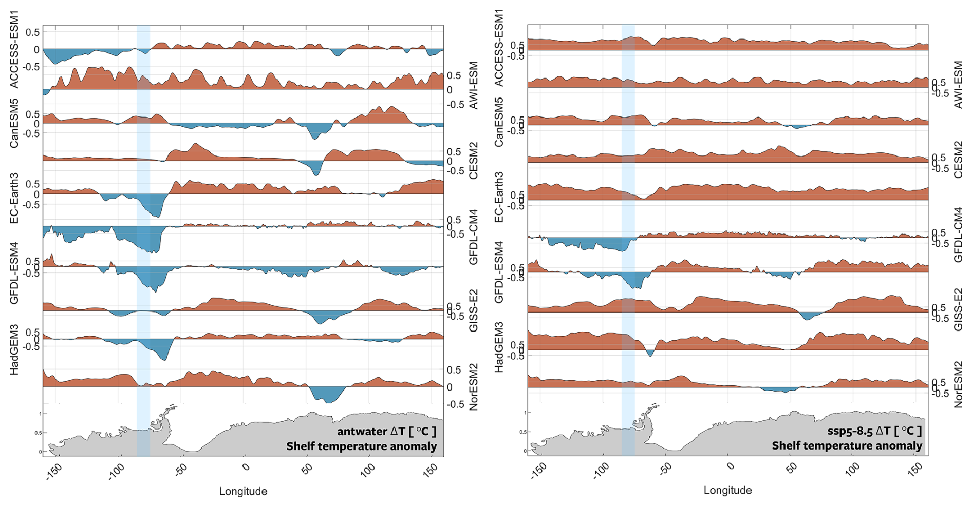
Figure 7 Circum-Antarctic mean shelf temperature change (0-bottom, poleward of the 1000 m isobath until the ice shelf front) in response to meltwater perturbation (antwater–piControl, comparing the last 10 years; left) and under SSP5-8.5 (comparing 2090–2100 with 2015–2025; right) for all models. Note the different scales on the y axis for the different models. Shaded regions indicate the Bellingshausen sector, where multiple models show negative anomalies, which are examined in detail later in the paper.

3.2 Warming or Cooling on the Continental Shelf

A key question for assessing potential melting feedbacks is whether offshore anomalies propagate onto the continental shelf and how they influence temperatures at the ice shelf front. Figures 7 and 8 present the volume-averaged continental shelf temperature anomalies from both the antwater and SSP5-8.5 simulations as a function of longitude. Notably, these results differ markedly from the zonal mean volume-averaged anomalies shown in Fig. 3c, highlighting the importance of regional variability. Taking into account the varying magnitude of the anomalies in different models (different scaling of the y axis in Fig. 7a), a consistent pattern emerges in the antwater simulations: warming anomalies dominate the Weddell Sea and much of the East Antarctic shelf, while cooling anomalies appear west of the Antarctic Peninsula in $\mathrm{6}/\mathrm{10}$ models with additional two models show weaker than zonally averaged warming. Warming anomalies typically reach up to 0.5 °C, while cooling anomalies range from −0.5 °C to as low as −1.5 °C, with the strongest cooling observed in the GFDL models. In contrast, the SSP5-8.5 simulations exhibit a more uniform warming signal along the Antarctic shelf. Shelf temperature anomalies under SSP5-8.5 typically reach up to 1 °C, reflecting the cumulative effects of long-term global warming.

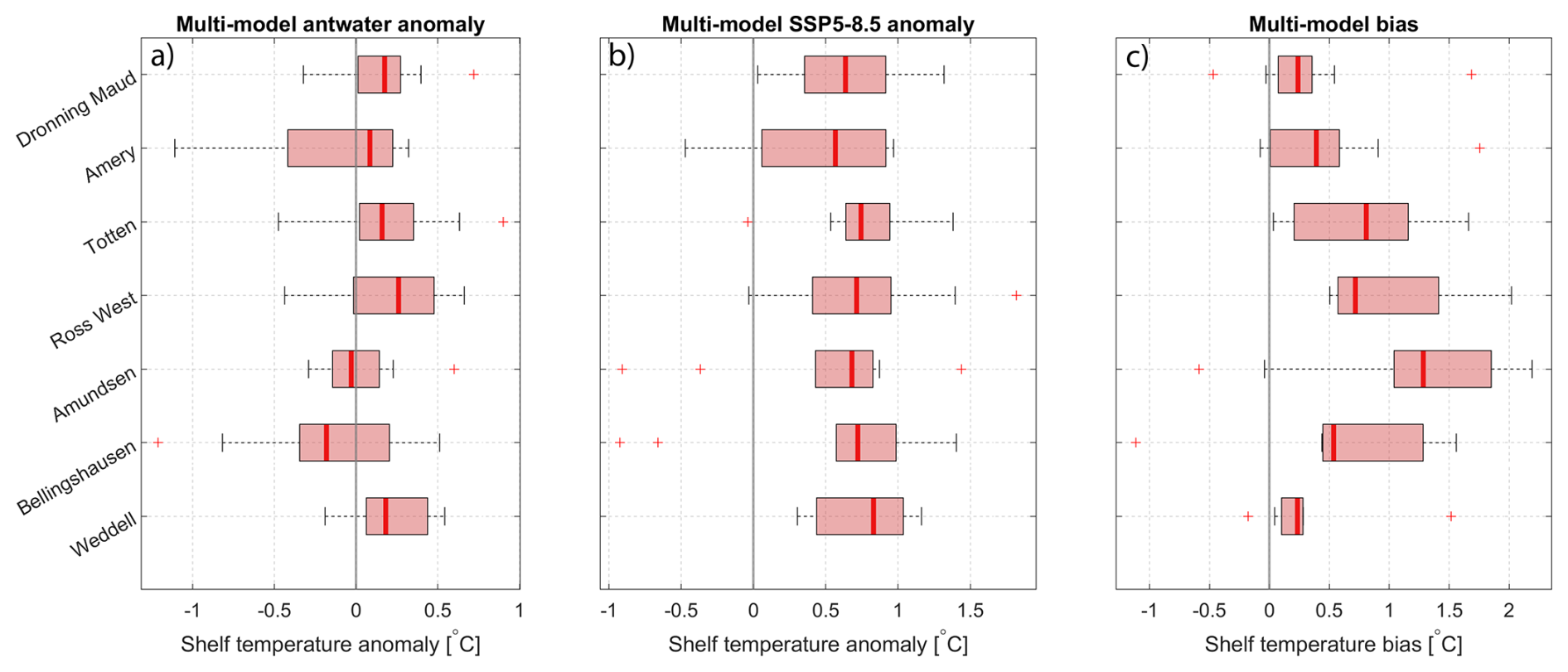
Figure 8 Box plots of shelf (0-bottom, poleward of the 1000 m isobath to the ice shelf front) temperature anomalies for all models combined in the regions defined in Fig. 1. The rectangle represents the second and third quartiles of all models, the red line indicates the multi-model median value, and the whiskers show the maximum model spread. Red plus signs indicate outliers (values beyond 1.5 times the interquartile range from the quartiles). The left column shows the multi-model temperature change due to meltwater perturbation (antwater – piControl, comparing the last 10 years), the second column illustrates the multi-model temperature change under SSP5-8.5 (comparing 2090–2100 with 2015–2025), and the third column shows the multi-model bias (piControl - observations).

The multi-model spread and median of continental shelf temperature anomalies across the regions defined in Fig. 1b are summarized in Fig. 8. Following the interquartile range, there is significant warming in response to antwater in Dronning Maud Land, Totten, Ross West and Weddell, while Amery, Amundsen and Bellingshausen are inconclusive. All show significant warming in SSP5-8.5. The Dronning Maud Land, Ross West, Totten, and Weddell regions show considerable multi-model median warming under antwater (0.17, 0.26, 0.16, and 0.18 °C, respectively), with even stronger warming under SSP5-8.5 (0.64, 0.65, 0.66, and 0.82 °C, respectively). In contrast, the Amundsen and Bellingshausen regions exhibit cooling in the antwater multi-model median. The Amery region is also notable for showing cooling or subdued warming anomalies in several models. Under SSP5-8.5, most models indicate warming, but both GFDL models still show cooling in the Amundsen and Bellingshausen regions, although other studies suggested that this signal may partly reflect internal variability within the model (Purich and England, 2021).

The cold anomaly in the Amundsen and Bellingshausen regions in response to meltwater was previously reported by Beadling et al. (2022) for the GFDL models in response to experiments similar to those studied here (0.1 Sv non-spatially-uniform forcing), but we now show that this feature is evident in $\mathrm{6}/\mathrm{10}$ of the SOFIA simulations. The mechanisms driving this cooling west of the Antarctic Peninsula are explored in Sect. 4.3, but in particular these regional patterns do not align with the piControl temperature distribution, which features the warmest waters in West Antarctica (not shown). Among models that do not show a distinct cooling anomaly in West Antarctica, CESM2 and NorESM2 exhibit reduced warming, suggesting that similar mechanisms may be at play, but to a lesser extent. Furthermore, both GFDL models show a cooling anomaly in West Antarctica under SSP5-8.5, implying that comparable processes may be influencing both experiments. However, in SSP5-8.5, the signal may be weaker, masked, or offset by the general warming of the Southern Ocean under global warming scenarios. The Amery region also exhibits a cold anomaly or, at minimum, a subdued warming response in several models under antwater, although the multimodel median remains positive.

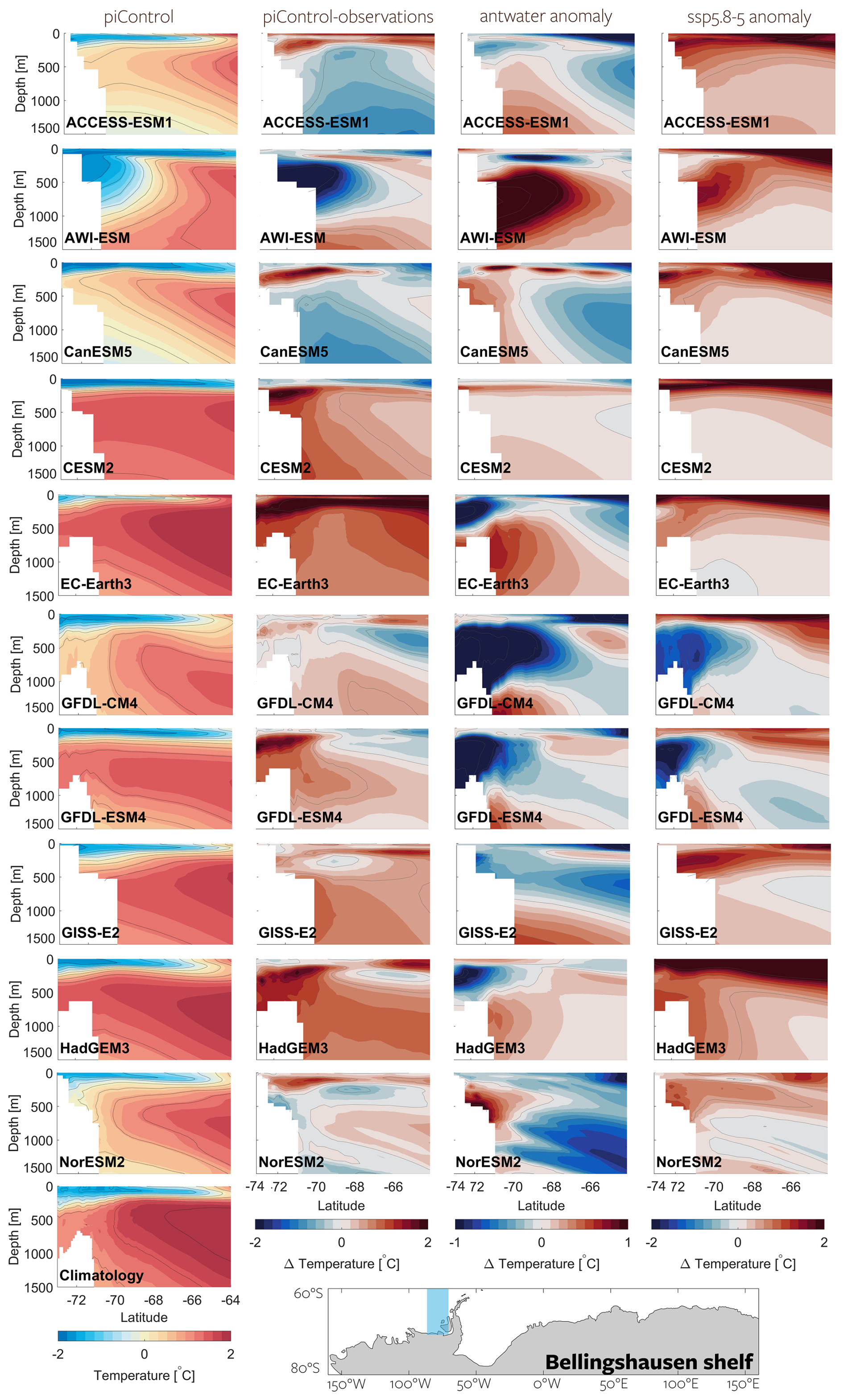
Figure 9 Example transect of the Bellingshausen region, where the shelf temperature response to an additional meltwater forcing is negative, contrasting with other regions. The first column presents the model's climatological mean temperature in the upper 1500 m, extending northward from the continental shelf. The second column shows the bias (piControl – observations), the third column displays the temperature change due to meltwater perturbation (antwater – piControl, comparing the last 10 years), and the fourth column illustrates the temperature change under SSP5-8.5 (comparing 2090–2100 with 2015–2025). Note that all data are plotted on the model's native grids, displaying varying horizontal and vertical resolutions and shelf extents (except AWI-ESM, whose native grid is unstructured). However, detailed bathymetry from each model is not shown. The observational climatological mean is shown at the bottom.

The intermodel spread varies considerably across regions, with the Bellingshausen and Amery regions standing out as having the largest overall spread. The pronounced intermodel variability, along with the multimodel median cooling response, highlights the need for further investigation of the Bellingshausen region. Figure 9 presents vertical sections of all models on the Bellingshausen shelf, illustrating the vertical and horizontal extent of these anomalies and their relationship to model biases in this region.

The Bellingshausen continental shelf is classified as a “warm” shelf regime (Thompson et al., 2018), characterized by the presence of a relatively warm and salty unmodified CDW on the continental shelf, and the absence of a pronounced ASF. Most models capture this direct isopycnal connection between the shelf and the deep ocean (first column, Fig. 9) and simulate warm waters reaching the coast. However, AWI-ESM stands out as the only model without a warm shelf regime here, consistent with its unique response to antwater compared to the other models (third column, Fig. 9). Although offshore temperature structures and mean states are relatively consistent across models, they differ in the southward extent of CDW intrusion and the steepness of temperature gradients near the shelf break. Some models (ACCESS-ESM1, GFDL-CM4, GISS-E2, HadGEM3, NorESM2) exhibit a distinct slope front, while others display flatter isotherms extending southward. The biases are generally the largest on the shelf and the lowest offshore, with most models showing a warm bias compared to the climatology in this region.

Models that exhibit a cold on-shelf response to antwater generally show the anomaly extending throughout most of the water column, from the shelf break toward the continent. However, the vertical and horizontal structure of this cooling varies across the ensemble, and in several models the signal is weak, confined to shallow layers, or offset by subsurface warming. Under SSP5-8.5, most models show robust upper-500 m shelf warming, though the GFDL models retain localized cooling. This suggests that the mechanisms contributing to the antwater cooling response may also modulate the SSP5-8.5 shelf response (see Sect. 4.3).

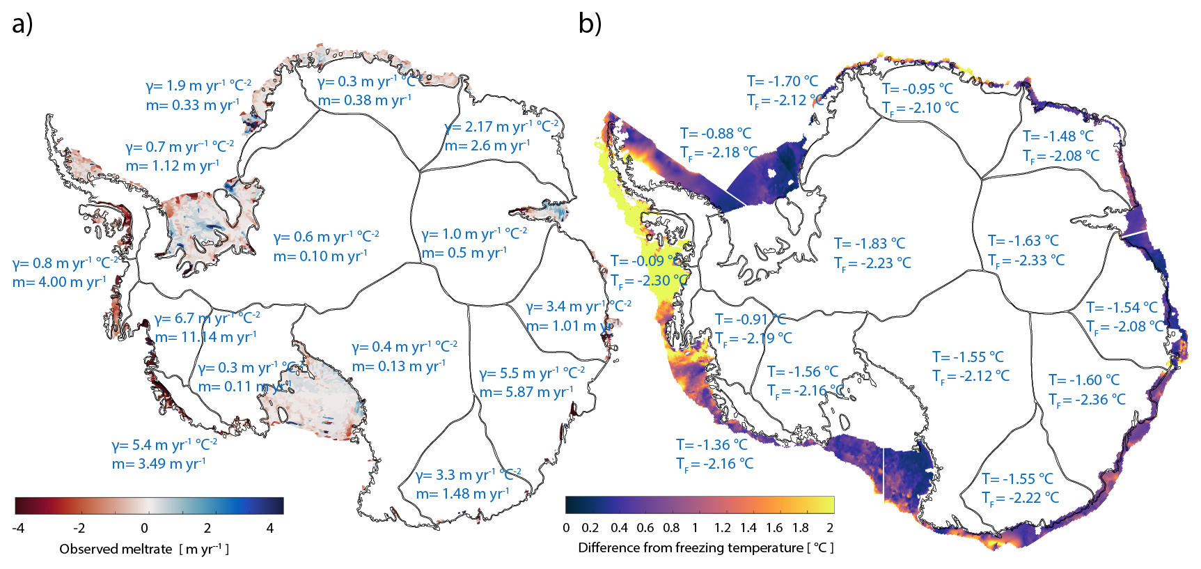
Figure 10 (a) Observed 1992–2017 mean basal melt rates (from Paolo et al., 2023) shown in color shading. Values represent regional mean melt rates and the γ coefficient, which is derived using the local quadratic melting parameterization, as described in Eq. (2). (b) Shelf thermal forcing (defined as the temperature above the local freezing point; colorbar), along with regional mean values of shelf temperature (T) and freezing temperature (T_f) at the depth of the ice shelf base (based on the spatially averaged ice shelf draft; see Sect. 2.5). Regions are defined as areas poleward of the 1000 m isobath extending to the ice shelf front. Temperature data are from observations (Sect. 2.3; Zhou et al., 2026).

3.3 Present Day Melt Rates and Regional Parameterizations

Following the approach of Jourdain et al. (2020), we translate simulated ocean temperature anomalies into basal mass loss anomalies (Sect. 2.4). Due to significant biases in the mean temperatures modeled around the Antarctic coast (Sect. 3.1), we use updated observationally-based climatology and updated satellite-derived basal melt rate estimates to calibrate the basal melt parameterization. Satellite-derived temporal mean basal melt rates for 1992–2017 are presented in Fig. 10a, with values representing the spatial mean for each IMBIE region.

Figure 10b presents the temporally averaged thermal forcing (Sect. 2.3), calculated from observational climatology, across the continental shelf from the 1000 m isobath to the ice shelf fronts (except in the Weddell and Ross regions where the northern boundary has been moved southward to account for the large shelf area). The values reflect the regional mean shelf temperatures (T) and the reference melting point temperatures (T_f) at the respective mean ice shelf drafts (Sect. 2.5). Thermal forcing is highest in the warm regions of West Antarctica, reaching up to 2.21 °C, while it remains relatively low in East Antarctica, typically ranging between 0.57 and 1.15 °C. Despite incorporating more recent data than other climatological datasets, the climatology remains subject to uncertainty and potential subsampling of temporal variability. For example, the estimated shelf temperatures in Dronning Maud Land ($T=-\mathrm{0.95}$ °C) are probably overestimated compared to Hattermann et al. (2012), Lauber et al. (2024), whereas they are likely underestimated in the Amundsen Sea ($T=-\mathrm{0.91}$ °C) compared to the observational estimates from Jenkins et al. (2010), Nakayama et al. (2019). Nonetheless, we use this temperature dataset throughout the analysis to ensure consistency across regions.

The regional melt-rate coefficients γ_j (Eq. 2) span a wide range (Fig. 10a). However, the spatial average γ_j is 2.1 m yr⁻¹ °C⁻², closely aligning with the spatial mean of 2.2 m yr⁻¹ °C⁻² suggested by Jourdain et al. (2020). These results highlight the considerable spatial variability in melt sensitivity, while also reflecting substantial uncertainty. Specifically, this uncertainty arises from the potential overestimation of thermal forcing in climatology and the inherent limitations in the formulation of melt rate parameterizations (Burgard et al., 2022).

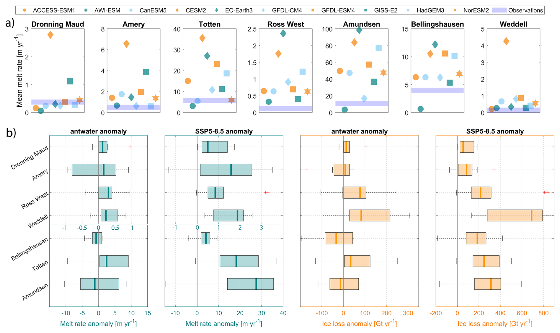
Figure 11 (a) Simulated mean melt rates (piControl) calculated using Eqs. (1) and (2) with simulated ocean temperatures and γ values from Fig. 10, compared with observed melt rates for regions defined in Fig. 1. (b) Box plots of multi-model simulated melt rate anomalies (left panels) and total ice shelf mass anomaly due to basal melt (right panels) for the same regions as in (a), based on meltwater experiments and under SSP5-8.5. Note different x axis scales for the melt rates in the Amundsen, Totten, and Bellingshausen regions. The rectangle represents the second and third quartiles of all models, the thick colored line indicates the multi-model median anomaly, and the whiskers show the maximum model spread. Melt rates are calculated using the calculated γ values and simulated temperature anomalies from Fig. 10.

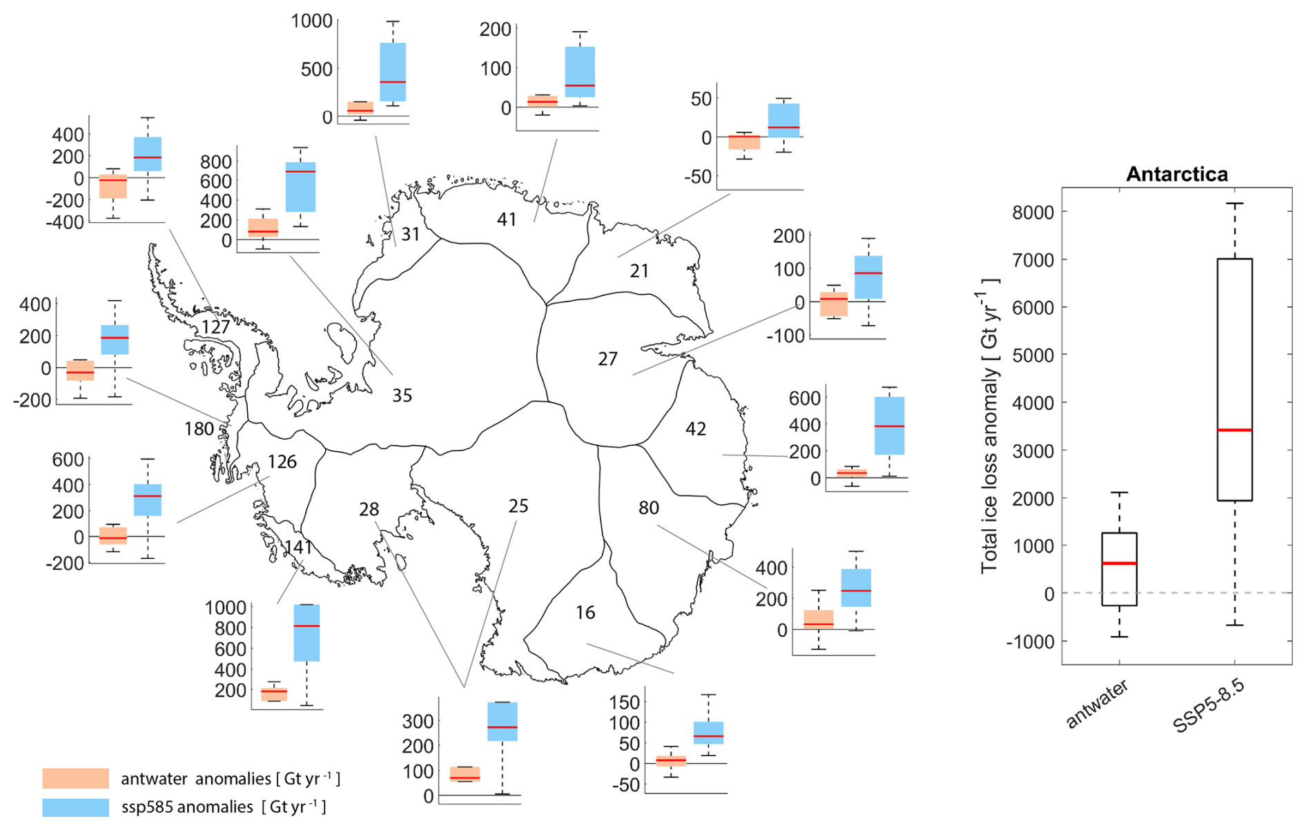
Figure 12 Map of Antarctic regions with box plots of multi-model anomalies of total ice shelf mass loss (melt rates multiplied by total ice shelf area) in response to the antwater experiments (orange) and under SSP5-8.5 (blue). Values on map indicate observed ice loss in Gt yr⁻¹ (1992–2017). On the right, a box plot shows the sum of all regions, representing the total uncertainty in ice shelf mass loss along the entire Antarctic continent due to the oceanic basal melting feedback in the meltwater experiments (antwater – piControl, comparing the last 10 years) and under the SSP5-8.5 simulations (comparing 2090–2100 with 2015–2025).

3.4 Future Melt Rates and Projected ice shelf mass loss

To assess the impact of model biases on melt rates, we first calculate the mean melt rate using the uncorrected bias piControl model temperatures for our selected regions (top row in Fig. 11). In general, melt rates derived from piControl are overestimated by a factor of 2 to 6 compared to present-day observations. However, in some regions – such as Dronning Maud Land and the Weddell Sea – the agreement is notably better. These findings underscore the need for bias correction or the use of temperature anomalies alone, as recommended by Jourdain et al. (2020), when employing climate model temperature fields to estimate basal melt rates. It is important to note that piControl and observational estimates cover different time periods; the absence of anthropogenic warming in piControl should lead to underestimated melt rates. Future experiments will repeat this setup under historical and future scenario forcing (Swart et al., 2023). Nevertheless, the regional pattern in calculated melt rates corresponds well with observations – regions with low observed melt also simulate low melt rates, and vice versa (noting the different y axis scales) – indicating that the regionally dependent γ parameter performs as intended. Lastly, we note that salinity variations have a negligible impact on freezing temperature in this context, with pressure and temperature exerting far greater influence.

We now explore the melt rate anomalies resulting from the antwater and SSP5-8.5 simulations, shown in the lower panels of Fig. 11. Figure 11 illustrates both the anomalous melt rates (left panels) and the corresponding regional mass loss (right panels), obtained by scaling the melt rate anomalies by the total ice shelf area in each region. As anticipated, the difference in the melting anomalies between antwater and SSP5-8.5 closely mirrors the pattern of their respective warming anomalies, with the highest melting observed under SSP5-8.5. Negative temperature anomalies correspond to negative melting anomalies, underscoring the direct link between ocean thermal forcing and basal melting. For antwater, the multi-model median melt rate anomalies range from −0.8 m yr⁻¹ in the Bellingshausen region to +2 m yr⁻¹ in the Totten region, but typically with an order of magnitude greater variability between different models. Under SSP5-8.5, the multimodel median melt rate anomalies increase to vary from +0.5 m yr⁻¹ in the Dronning Maud Land region to +28 m yr⁻¹ in the Amundsen region. The basal melt rates of the mean state are overestimated (top panels, Fig. 11), likely due to warm biases in the simulations of the model (Fig. 8). However, it is also possible that the parameterization itself is overly sensitive, contributing to the overestimation. If this is the case, then the melt rates derived from the temperature anomalies (lower panels, Fig. 11) may also be overestimated.

Translating melt rate anomalies into total ice shelf mass loss highlights the important role of ice shelf area in shaping regional differences. A key caveat here is that we assume homogeneous basal melting across the ice shelf base, whereas in reality, melting is typically concentrated near the grounding line. Unlike temperature anomalies (Fig. 8), total ice shelf mass loss patterns are influenced by both the sensitivity to thermal forcing and the spatial distribution of ice shelves. Under antwater, ice shelf mass loss varies from −40 Gt yr⁻¹ in the Bellingshausen region to +80 Gt yr⁻¹ in the Weddell region, while SSP5-8.5 simulations indicate a range from +55 Gt yr⁻¹ in Dronning Maud Land to +690 Gt yr⁻¹ in the Weddell. This pattern aligns with observations (Fig. 10), where high melt rates in the Totten region contribute less to total ice shelf mass loss due to its relatively small ice shelf area, while the Weddell region experiences the highest mass loss, reflecting its extensive ice shelf coverage.

The multimodel median and spread of these total ice shelf mass loss anomalies in all IMBIE regions are summarized in Fig. 12, providing a pan-Antarctic perspective on regional disparities. This figure demonstrates the accumulated uncertainty and the large regional differences in the loss of mass on the Antarctic ice shelf due to global warming (SSP5-8.5) and meltwater (antwater) feedbacks. These differences are shaped by a combination of regionally varying ocean temperature anomalies, ice shelf area, and variations in melt sensitivity, highlighting the intricate and uncertain nature of Antarctica's future mass balance.

4 Discussion

4.1 Does an Asymmetric Temperature Response Lead to a More Symmetric Ice Shelf Mass Loss Around the Continent?

Likely, yes: a more symmetric pattern emerges because cooling anomalies reduce melt in parts of West Antarctica, while East Antarctica, traditionally a cold-shelf region, shifts toward a warm-shelf regime and contributes more strongly to total mass loss. Present-day observations indicate that West Antarctica currently dominates basal melt–driven ice shelf mass loss, and recent modeling studies predict that continued increases in West Antarctic melt are unavoidable (Naughten et al., 2023). However, both the antwater and SSP5-8.5 simulations suggest that future ice shelf mass loss could become more evenly distributed around the continent. This emerging pattern aligns with evidence that East Antarctica may be more vulnerable to future warming and melt than previously assumed (Herraiz-Borreguero and Naveira Garabato, 2022). Although both experiments exhibit widespread subsurface warming, the antwater cooling response west of the Peninsula produces an asymmetric temperature pattern along the continental shelf (Fig. 7a). This redistribution is clearly illustrated in Fig. 13b, where adding the antwater anomalies to present-day melt rates shows the increasing relative contribution from East Antarctica as cooling suppresses melt in parts of West Antarctica.

Currently, the highest ice shelf mass loss occurs in the Bellingshausen sector (see sector definitions in Fig. 1b). However, when antwater anomalies are incorporated, the F-G sector (between the Amundsen and Ross Seas) emerges as the largest contributor, with the Totten and Weddell regions also gaining importance. In contrast, the Ap-B, Eastern Ross, and Amery sectors comparatively small contributors. In particular, the increasing importance of the F-G region is striking, as it shares a similar warm continental shelf with the Bellingshausen and Amundsen sectors in today's climatology, but it is not affected by the cooling anomalies that develop in those sectors under antwater.

A similar, though weaker, pattern emerges under SSP5-8.5. Some models exhibit an east–west asymmetry in temperature anomalies, with reduced warming in West Antarctica (Fig. 7b). When median SSP5-8.5 anomalies are added to present-day melt rates, East Antarctica and the Weddell sector show melt rates comparable to those in the Bellingshausen and Amundsen sectors, and the F–G sector again emerges as the largest individual contributor. The Eastern Ross, Ap–B, and Amery sectors remain among the smallest contributors in both experiments.

These regional responses are strongly model-dependent, particularly in antwater. Models that exhibit a strong negative feedback from meltwater in West Antarctica dominate the multi-model median, while others – such as AWI-ESM, show no cooling at all. The cause of these differences remain unclear, but differences in model physics likely contribute: for example, AWI-ESM is the only model using an unstructured mesh and does not display the warm-shelf regime in the Bellingshausen sector seen in most other models (Fig. 9). Model dependency is further exemplified by comparing our results with those of Naughten et al. (2023). Their CESM1-forced regional model projects strong Amundsen Sea warming (1.39 °C) in the Amundsen Sea region under RCP8.5. This is broadly consistent with our ensemble: the third quartile spans 0.5–1.0 °C under SSP5-8.5, and CESM2 – the successor to CESM1 – simulates a warming of 0.55 °C in this region (Fig. 8b), lower than the CESM1 estimate. Among the models considered, CESM1 therefore provides a high-end projection of shelf warming. The model used by Naughten et al. (2023) includes ice-shelf basal melt and the associated heat and freshwater fluxes, but is not coupled to an ice sheet and therefore does not account for additional freshwater input from ice sheet runoff. As such, it cannot capture the freshwater-induced continental shelf warming/cooling feedback investigated in our antwater experiment. Even if this feedback were included, CESM2 does not simulate a negative feedback in this region under antwater, suggesting that CESM1 may not either. Hence, as noted by Naughten et al. (2023), it remains uncertain whether CESM1 over- or underestimates future freshening and associated warming. This does not suggest that continued warming in the Amundsen Sea is unlikely. However, given that several models in our ensemble project a potential negative feedback in response to additional meltwater, and considering that CESM1 produces stronger regional warming than most models, it is plausible that future warming in this region may be somewhat lower than the CESM1-based estimate.

Additional processes may further shape these regional patterns. For example, in regions where meltwater induces cooling, including ice shelf feedbacks would likely reduce melt rates, thereby weakening the freshening that initially drives the cooling – highlighting the complex and nonlinear nature of ocean–ice shelf interactions. Moreover, climate-change-driven shifts in other freshwater sources not included in the antwater experiments, such as increased iceberg calving, altered sea ice melt and growth patterns, and regional variations in ice sheet surface mass balance, may substantially alter the spatial distribution of freshwater (as shown by Lockwood et al., 2021; Goddard et al., 2017) and thus modulate regional ocean warming or cooling.

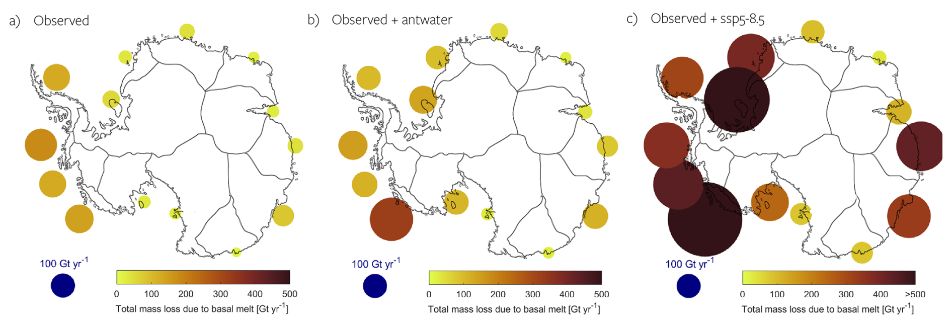
Figure 13 Map of Antarctic regions showing regional differences in total ice shelf mass loss due to basal melting: (a) observed, (b) observed plus multi-model median anomalies from meltwater perturbation experiments (antwater – piControl, comparing the last 10 years), and (c) observed plus multi-model median anomalies from the SSP5-8.5 scenario (comparing 2090–2100 with 2015–2025).

4.2 Does Meltwater Discharge Amplify or Suppress Global Warming-Induced Continental Shelf Warming?

Our results show that Antarctic meltwater discharge can either amplify or suppress global warming–induced shelf warming, and the sign of the response varies by region and model. Because the meltwater-driven and greenhouse-driven anomalies are of comparable magnitude, the net effect is strongly model- and region-dependent.

Anomalies of ice shelf basal melting under SSP5-8.5 exhibit substantial uncertainty (Fig. 12). Integrated across Antarctica, the multi-model median indicates an additional +3300 Gt yr⁻¹ melt by the end of the century, but the full range spans from −800 to +7900 Gt yr⁻¹, reflecting the wide spread in ocean warming. Notably, some models still simulate a net reduction in ice shelf mass loss (negative anomalies) despite the strong SSP5-8.5 warming.

The magnitude of the meltwater-driven response is similarly variable. Under preindustrial control conditions, the multi-model median antwater anomaly is approximately +750 Gt yr⁻¹, with individual models ranging from negative values to increases of nearly +1900 Gt yr⁻¹. For context, the current observed ice shelf mass loss from basal melting is about 1000 Gt yr⁻¹ (Rignot et al., 2019; Paolo et al., 2023; Davison et al., 2023). This highlights that meltwater feedbacks can either reinforce or counteract the SSP5-8.5 warming signal and are large enough to alter regional melt patterns substantially.

Because the antwater and SSP5-8.5 responses arise from different forcings, their impacts are not linear and cannot be assumed to be additive. Fully constraining their combined effect therefore requires scenario experiments that explicitly include meltwater forcing – such as the Tier 2 simulations proposed in the SOFIA experiment (Swart et al., 2023).

Although the net outcome remains uncertain, our results suggest that if the feedbacks seen in antwater also operate under SSP5-8.5, warming may be dampened in regions with a negative feedback and amplified where a positive feedback dominates. Because both signals are of comparable magnitude, their interaction is likely to be significant, with important implications for future Antarctic ice shelf change.

4.3 Is Cooling in West Antarctica Driven by Regional Ocean Connectivity?

Likely yes. In models that exhibit cooling along the West Antarctic shelf, the signal is consistently linked to enhanced westward advection of cold, fresh Weddell Sea waters via a strengthened ASC/ACoC system. However, this mechanism is not universal across models, reflecting differences in mean state biases and regional circulation responses.

Despite the uniformly applied meltwater perturbation in antwater, models differ substantially in their coastal temperature responses, raising the question of whether certain underlying mechanisms are active in some models but absent in others. In particular, the cooling anomaly in west Antarctica is evident in 6 of 10 models, but not all, underscoring considerable uncertainty in how the ice shelves in this region will respond to increased freshwater input. High-resolution simulations with ACCESS-OM2-01 (Moorman et al., 2020) demonstrate that meltwater-induced freshening can intensify along-slope and along-shelf density gradients, strengthening the westward ASC and ACoC and advecting cold Weddell Sea waters into the Bellingshausen and Amundsen Seas. Similar interpretations have been proposed in other meltwater perturbation studies (Beadling et al., 2022; Tesdal et al., 2023). This advective pathway from the Weddell Sea around the Antarctic Peninsula has been identified in earlier work (Heywood et al., 2004), mapped with Lagrangian particles (Dawson et al., 2023), and supported by seal-mounted CTD observations that trace the route into the Bellingshausen Sea (Schubert et al., 2021).

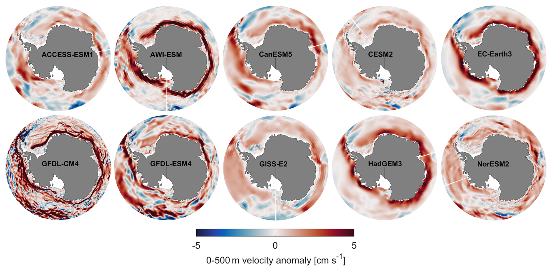
Figure 14 Spatial anomalies of vertically averaged (0–500 m) along-slope velocity (cm s⁻¹, with positive values indicating westward flow) in response to the meltwater perturbation experiments (antwater – piControl, comparing the last 10 years). Red values indicate a strengthening of westward currents (e.g., the along-slope Antarctic Slope Current (ASC) and on-shelf Antarctic Coastal Current (ACoC)), while blue values indicate a weakening of westward currents or a strengthening of eastward currents. 0–500 m is chosen as this is the vertical extent because this depth range corresponds to the core of the ASC in the models.

Our results support this interpretation: across the multi-model ensemble, strong cooling along the West Antarctic shelf generally coincides with ASC intensification. The spatial anomaly of along-slope velocity (Fig. 14) shows a pronounced strengthening of the westward ASC near the shelf break, and models with the strongest intensification also tend to show the most pronounced cold anomalies (except AWI-ESM). This could also represent a positive feedback, where a strong mean-state ASC traps more freshwater near the coast, further strengthening the ASC.

However, ASC strengthening alone does not fully explain the presence or absence of coastal cooling. For example, some models that do not show a cooling anomaly in the Bellingshausen or Amundsen regions – such as AWI-ESM, CanESM5, CESM2, and NorESM2 (Fig. 4a), also display a strengthened ASC. This discrepancy may arise from differences in the mean state. For instance, Fig. 9 shows that AWI-ESM does not feature a warm regime on the West Antarctic shelf to begin with, instead exhibiting a substantial cold bias. Additionally, differences in how models simulate the response to antwater in the Weddell Sea could influence the advection of anomalies, further affecting regional responses.

In Moorman et al. (2020), Beadling et al. (2022), Tesdal et al. (2023) cold anomalies along the West Antarctic shelf coincide with reduced DSW production in the Weddell Sea. This shift involves a transition from dense shelf water formation to the production of lighter dense waters that are too buoyant to overflow from the continental shelf and cascade to the ocean bottom. This enables cold, fresh Weddell waters to be advected westward around the Antarctic Peninsula into the Bellingshausen and Amundsen Seas. Assessments of seawater age in these studies further support this mechanism, with recently ventilated waters appearing in West Antarctica. If this mechanism is active in our ensemble, the cooling west of the Antarctic Peninsula should be accompanied by negative bottom age anomalies, indicating replacement of older CDW by recently ventilated Weddell waters.

Although not all models provide seawater age, those that do show a clear relationship between bottom age anomalies and regional cooling (Fig. 15). Several models exhibit pronounced negative bottom age anomalies in West Antarctica, consistent with strong cooling, while others show weaker or even positive anomalies, matching their muted or warm responses. These patterns support the idea that cooling west of the Antarctic Peninsula reflects the westward advection of recently ventilated Weddell Sea waters. Fully confirming this mechanism, however, will require detailed investigation of the water mass transformation processes and DSW production, which will be the focus of a future study.

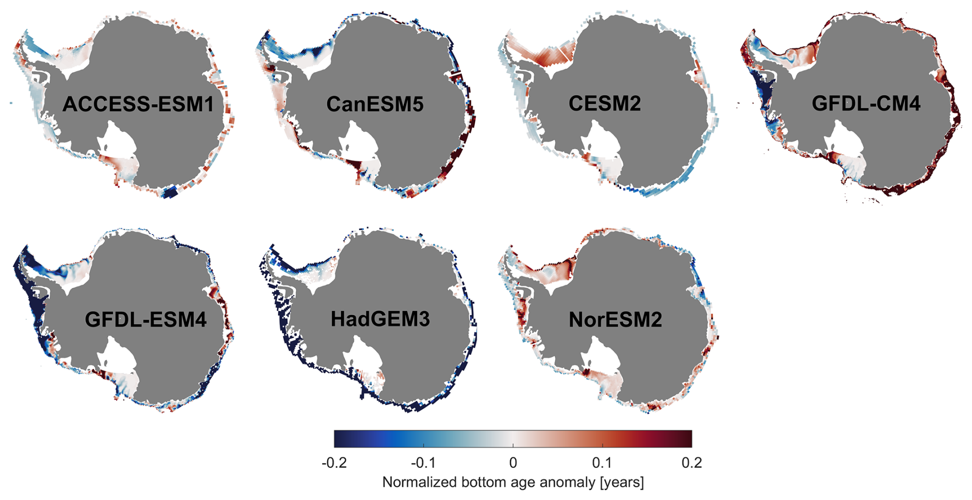
Figure 15 Spatial bottom age anomaly (years since surface contact) along the Antarctic shelf (southward of the 1000 m isobath) for the last 10 years of the antwater experiment. To normalize, the mean bottom age at each grid cell is divided by the spatial mean bottom age in the Southern Ocean (south of 30° S and deeper than 4000 m) from the piControl simulations. Negative values mean older water is being replaced by more recently ventilated water, and positive values indicate less ventilation of bottom waters. Adapted from Beadling et al. (2022), Fig. A3. The variable “agessc” was not available for the AWI-ESM1, EC-Earth3, and GISS-E2 models.

4.4 A combination of uncertainties from multiple factors

In the Introduction, we identified multiple factors contributing to uncertainty in simulating basal melting feedbacks: (a) model-dependent climate responses and feedbacks to meltwater discharge, (b) the complex interactions between the open ocean and the continental shelf, (c) uncertainties in basal melt parameterizations due to limited observations, (d) the interplay between meltwater-induced and global warming-driven changes, and (e) biases in climate models' representation of Southern Ocean water masses and near-shelf dynamics.

Our results show that the model spread in total ice shelf mass loss under antwater and SSP5-8.5 reflects the combined effect of all these uncertainties. This highlights the challenge of reliably downscaling and projecting future coastal ocean conditions that will influence Antarctic ice shelf mass loss. While we cannot isolate the dominant source of uncertainty, we can provide insights into each contributing factor and offer recommendations for future research:

• a.

  Multi-Model Perspectives on Meltwater Response.
  The SOFIA multi-model ensemble provides, for the first time, a direct comparison of how different climate models respond to identical meltwater forcing. Our results reveal consistent large-scale responses, including deep-ocean warming and shelf warming in some regions while others experience cooling. However, substantial differences exist in both magnitude and regional distribution. This finding reinforces the importance of using multi-model ensembles rather than relying on single-model interpretations, similar to other climate model studies. Other alternatives to large model ensembles are to evaluate models against observations and select those that best represent Southern Ocean conditions (e.g., Barthel et al., 2020), or to avoid models that are outliers in their response to either meltwater or global warming. The intermodel spread in temperature anomalies remains a significant source of uncertainty in projected ice shelf mass loss.

• b.

  Regionality of Meltwater Feedbacks.
  First and foremost, our results show that meltwater and global warming responses are highly regionally dependent. Zonal averages can be misleading and are inappropriate when considering changes along the different continental shelf regimes (Thompson et al., 2018). By analyzing regional responses, we reduce the uncertainties inherent in studies using zonal averages. For example, previous studies have suggested that the basal melting feedback to meltwater is predominantly positive (e.g., Bronselaer et al., 2018), which is accurate for the open-ocean Southern Ocean as a whole but not for individual shelf regimes (Figs. 5 and 6). Our findings also emphasize that local continental shelf dynamics – including slope front changes, deep shelf water (DSW) production, and strengthening of the Antarctic Slope Current (ASC) or Antarctic Coastal Current (ACoC) – are key to understanding meltwater impacts. Simply extrapolating offshore ocean properties onto the continental shelf is, therefore, inadequate. Instead, regional connectivity and advective pathways (Dawson et al., 2023) must be considered. We thus recommend that future studies avoid zonal mean approaches and instead focus on regional responses on the continental shelf when assessing ice-ocean interactions. Additionally, similar to findings by Tesdal et al. (2023) and Beadling et al. (2022), we find that coarse-resolution climate models (all in this study, except GFDL-CM4) poorly represent shelf break dynamics, likely influencing their simulated responses. This underscores the critical role of model resolution in capturing key feedbacks and highlights the importance of assessing whether models adequately resolve features such as the ASC and DSW formation, both of which strongly affect freshwater retention and the strength of ocean–ice feedback mechanisms.

• c.

  Uncertainty in Basal Melt Parameterization.
  Despite recent advances, basal melt parameterizations (Jourdain et al., 2020) remain a key source of uncertainty. Recent studies suggest that a quadratic relationship provides a reasonable approximation (Burgard et al., 2022), but a major challenge lies in the availability of unbiased observational data. For instance, overestimated temperatures in Dronning Maud Land and underestimated temperatures in the Amundsen Sea (Sect. 3.3) influence the inferred melt rate coefficient γ, leading to uncertainties in mass loss estimates. Nevertheless, the updated climatology used in this study incorporates the most comprehensive observational datasets to date, including marine mammal-derived measurements from beneath ice shelves. As a result, this climatology likely introduces fewer biases than global ocean products, which are known to have significant errors (Jourdain et al., 2020). A key takeaway from our work is the importance of regionally calibrated melt rate parameterizations rather than assuming a uniform γ across Antarctica, supporting findings from Jourdain et al. (2020) and Lambert et al. (2025). Additionally, as observational ocean climatologies are updated, they should be paired with updated basal melt rate datasets (e.g., Paolo et al., 2023) to ensure consistency.

• d.

  The Interaction Between Meltwater and Global Warming.
  Understanding the combined effects of meltwater discharge and global warming remains a challenge. Our comparison of antwater and SSP5-8.5 simulations provides insights into the consistency (or lack thereof) in their respective impacts on basal melting. However, caution is needed when interpreting these comparisons. While SSP5-8.5 does not explicitly include meltwater forcing, the two experiments cannot simply be summed due to potential nonlinearities and missing feedbacks. Nevertheless, comparing these scenarios offers insight into whether their effects are likely to amplify or counteract each other. Future experiments, such as the Tier 2 SOFIA simulations, which include both greenhouse gas forcing and additional meltwater (Swart et al., 2023), will provide a clearer picture of the combined effects. One key takeaway from our work – relevant for future Tier 1 vs. Tier 2 comparisons – is that the SSP5-8.5 simulations already include additional freshwater input through enhanced hydrological cycle and increased P−E. This freshwater input, which is comparable in magnitude to the 0.1 Sv forcing used in antwater, suggests that similar mechanisms may be active in both experiments, albeit masked or counteracted by competing warming trends.

• e.

  The Role of Model Bias.
  Model biases remain a major source of uncertainty in projecting future Antarctic mass loss (Barthel et al., 2020). Our results confirm that climate models struggle to accurately represent Southern Ocean water masses, with biases in the mean state also affecting responses to warming and meltwater perturbations. Additionally, biases in piControl climate simulations are often larger than the temperature anomalies driven by meltwater and nearly as large as those projected under high-emissions scenarios by the end of the century (Figs. 3b, c, and 8c). These findings underscore the need for a multi-model perspective in future studies. Improving the representation of Southern Ocean mean-state properties should also be a high priority for the climate modeling community. Antarctic water mass biases are particularly relevant when using global climate models to force regional simulations. We highly recommend evaluating models against observational datasets wherever possible and using caution when extrapolating real-world behavior in regions where model biases exceed the magnitude of the forced climate change signal. At the same time, it is important to acknowledge uncertainties in the observational datasets themselves, the challenges of comparing different time periods (e.g., pre-industrial simulations with present-day observations), and the influence of internal variability, which may be undersampled in both models and observations.

4.5 Experimental caveats

While the SOFIA antwater experiment provides a valuable framework to assess the impacts of meltwater in the Southern Ocean, several simplifications should be considered when interpreting the results. A key limitation is that meltwater is evenly distributed across all grid cells adjacent to the Antarctic coast at the surface, whereas in reality, meltwater enters the ocean through a combination of basal melting, where freshwater is introduced at depth, and calving, where icebergs melt at the surface but often far from the coastline. Moreover, the input of Antarctic meltwater is not uniform between regions, with the highest contributions originating from the Amundsen and Bellingshausen Seas, where the ice shelf melt rates are most pronounced (Seroussi et al., 2020). The impact of the horizontal and vertical distribution of meltwater has been examined in individual modeling studies (e.g., Merino et al., 2018; Mackie et al., 2020a; Thomas et al., 2023), as has the inclusion of latent heat associated with freshwater perturbations (Thomas et al., 2023), highlighting their critical role in shaping regional ocean responses. For example, using the SOFIA simulations, Kaufman et al. (2025), show that Southern Ocean SST trends are more sensitive to freshwater fluxes concentrated along the Antarctic margin versus more spatially distributed fluxes. The Tier 3 SOFIA experiments (Swart et al., 2023) will explicitly test the influence of the spatial distribution of the meltwater and the latent heat effects, providing a more refined understanding of these processes. Another important consideration is that the experiment accounts only for the freshening effect of meltwater, while neglecting the heat loss associated with adding water at the local freezing point and the latent heat loss due to melting. Previous studies (e.g., Hattermann and Levermann, 2010) suggest that this omission could lead to an underestimate of ocean cooling feedbacks. Finally, while biases in modeled ocean properties have been discussed, climate drift in long simulations is not explicitly accounted for, and natural internal variability within the models may also influence the results. For instance, it is possible that specific events – such as episodes of deep convection or variability in the tropical Pacific – may be subsampled, potentially contributing to the signals observed, as suggested by Purich and England (2021).

5 Conclusions

Using the SOFIA Tier 1 ensemble, we examined the ocean's response to a 0.1 Sv meltwater perturbation (antwater) and the resulting feedback on basal melting. Although meltwater feedback is generally thought to amplify basal melting, our results show that its impact varies regionally, enhancing basal melting in some sectors while suppressing basal melting in others. The multimodel median reveals a warming feedback on the continental shelf in most regions. In West Antarctica, however, the ensemble response differs markedly: several models simulate actual cooling of the continental shelf, while others show reduced (but still net positive) warming, particularly in the Bellingshausen and Amundsen Seas. A few models also indicate cooling in the Amery region. This highlights the limitations of zonal averages, which can obscure crucial regional differences across distinct continental shelf regimes, and aligns well with recent studies highlighting the importance of regional hydrography (Song et al., 2025).

The SOFIA simulations support existing hypotheses linking these asymmetric temperature responses to strong regional connectivity. Local shelf-break dynamics, including a strengthened Antarctic Slope Front (ASF) that limits Circumpolar Deep Water (CDW) intrusion, an accelerated Antarctic Slope Current (ASC) that advects anomalous Weddell waters, and reduced Dense Shelf Water (DSW) formation, play a crucial role in shaping regional responses. These processes are poorly resolved in coarse-resolution models, which likely affects their ability to simulate realistic meltwater-induced changes. This further implies that extrapolating offshore values onto the shelf is unrealistic, emphasizing the need for more refined approaches when assessing ice-ocean interactions.

A key question is how the effects of additional meltwater forcing compare to, and are modulated by, broader global warming–induced trends. While the SOFIA Tier 2 scenario experiments (Swart et al., 2023) – including added meltwater forcing under future climate conditions – are designed to address this, they are not yet available. In the meantime, by comparing the antwater experiments with SSP5-8.5 simulations – which reflect a wider range of global warming impacts, including substantial freshwater input from enhanced precipitation – we find that SSP5-8.5 generally produces a more spatially uniform warming along the Antarctic margin. On average, continental shelf warming is approximately three times stronger under SSP5-8.5 than under antwater. However, some models still exhibit cooling or reduced warming west of the Antarctic Peninsula, suggesting that similar mechanisms operate in both experiments but are masked or offset by competing warming trends in SSP5-8.5.

To translate these ocean temperature anomalies into basal melting, we updated and regionally calibrated a quadratic basal melt parameterization using a new regional ocean climatology and the most recent satellite-derived basal melt rates. This approach yields regional anomalies in ice shelf basal mass loss of the ice shelf from both the antwater and SSP5-8.5 simulations.

Integrated across the continent, the multimodel median suggests that the 0.1 Sv antwater forcing leads to an additional 750 Gt yr⁻¹ of ice shelf mass loss, while SSP5-8.5 simulations project an increase of 3400 Gt yr⁻¹ by the end of the century. For context, current observational estimates place ice shelf mass loss at approximately 1000 Gt yr⁻¹, indicating a potential 75 % increase driven by meltwater feedback alone and a 340 % increase under high greenhouse gas emissions.

However, substantial uncertainty persists, as the model spread represents a convolution of multiple sources of error, including biases in the model's mean state, limitations in the experimental design, poorly constrained melt parameterizations, and the complex interactions between the open ocean and diverse continental shelf regimes, which may not be adequately resolved in coarse-resolution climate models.

Despite these uncertainties, one consistent key finding emerges: in the West Antarctic regions where the greatest ice shelf mass loss has been observed in recent decades, most models project either cooling or reduced warming in the antwater simulation, indicating a dampening feedback due to meltwater input. This suggests that East Antarctica may become equally important in terms of future ice shelf basal mass loss, consistent with a broader shift “from cold shelf to warm shelf”. We therefore propose that the asymmetric temperature response to meltwater could drive a shift toward a more symmetric distribution of ice shelf mass loss across the continent – but at a higher overall rate. Future studies should assess whether reduced melt rates in West Antarctica could substantially lower the risk of marine ice sheet instability, which remains a key driver of high-end sea level rise projections from the West Antarctic Ice Sheet.