Mapping subsea permafrost around Tuktoyaktuk Island (Northwest Territories, Canada) using electrical resistivity tomography

Along much of the Arctic coast, shoreline retreat and sea level rise combine to inundate permafrost. Once inundated by seawater, permafrost usually begins to degrade. Tuktoyaktuk Island (Beaufort Sea, Northwest Territories, Canada) is an important natural barrier protecting the harbor of Tuktoyaktuk but will likely be breached within the next 2 decades. The state of subsea permafrost and its depth distribution around the island are, however, still largely unknown. We collected marine electrical resistivity tomography (ERT) surveys (vertical electrical soundings) north and south of Tuktoyaktuk Island using a floating cable with 13 electrodes in a quasi-symmetric Wenner–Schlumberger array configuration. We filtered the data with a new approach to eliminate potentially incorrect measurements due to a curved cable and inverted the profiles with a variety of parameterizations to estimate the position of the ice-bearing permafrost table (IBPT) below the seafloor. Our results indicate that north of Tuktoyaktuk Island, where coastal erosion is considerably faster, IBPT depths range from 5 m below sea level (120 m from the shoreline) to around 20 m b.s.l. (up to 800 m from the shoreline). South of the island, the IBPT dips more steeply and lies at 10 m b.s.l. a few meters from the shore, and 200 m from the shore, it is more than 30 m b.s.l. We discuss how marine ERT can be improved by accurately recording electrode positions, although choices made during data inversion are likely a greater source of uncertainty in the determination of the IBPT position. At Tuktoyaktuk Island, IBPT depths below the seafloor increase with distance from the shoreline; comparing the northern and southern sides of the island, the inclination is inversely proportional to coastline retreat rates. On the island's north side, the historical coastal retreat rate suggests a mean permafrost degradation rate of 5.3 ± 4.0 cm yr⁻¹.

1 Introduction

Coastal erosion and retreat have severe infrastructure and socioeconomic consequences in the Arctic (Irrgang et al., 2019; Ramage et al., 2021). They also transform permafrost from terrestrial to subsea, which may amplify erosion as it degrades (Solomon et al., 2008). In addition, the potential release of greenhouse gases from thawing permafrost might contribute to global warming as a positive feedback mechanism (Schuur et al., 2015), but despite the large subsea carbon stocks, the amount emitted to the atmosphere is still debated (Miesner et al., 2023). This study examines the use of a geophysical method to estimate the current degradation rate of ice-bearing subsea permafrost at Tuktoyaktuk Island (Beaufort Sea, Northwest Territories, Canada) and discusses potential sources of uncertainty that may arise from the survey design and technologies employed.

Subsea permafrost (the terms offshore, submarine or subaquatic can be used synonymously) is predominantly relic terrestrial permafrost formed during the Last Glacial Maximum (LGM) or earlier and inundated during marine transgression (Kitover et al., 2016). The occurrence of terrestrial permafrost is linked to the air temperature regime. In regions with a mean annual air temperature near the ground below 0 °C (or slightly above 0 °C because of the thermal offset effect), permafrost can form. This can be the case in polar regions (latitudinal permafrost) as well as in mountainous regions (altitudinal permafrost). Deep permafrost (several hundred meters) can last over centuries, even when mean annual air temperatures have risen above 0 °C. In contrast, subsea permafrost is bound to more specific conditions: the vast majority of subsea permafrost is relic terrestrial permafrost inundated during sea level rise. Heat and salt transfer from seawater thaws the permafrost from the top downwards; geothermal heat thaws it from below. Where relic permafrost is thick (several hundred meters), subsea permafrost can last over millennia. These conditions are met, for example, on the large Siberian Shelf, where subsea permafrost extends several hundred kilometers offshore, representing the largest subsea permafrost occurrence on Earth (Overduin et al., 2019; Obu et al., 2019). On a smaller scale, subsea permafrost can also be found along the Canadian coast, for example offshore of the Tuktoyaktuk Coastlands. Locally, subsea permafrost can also form in shallow waters when the water column freezes completely during winter (bottom-fast ice or bedfast ice), resulting in sub-zero benthic temperatures and freezing of the seabed sediment (Solomon et al., 2008). The seasonal presence of cryotic and/or frozen sediment on the seabed can be considered an active layer and has been observed in the Beaufort Sea near Prudhoe Bay, Alaska (Osterkamp et al., 1989). Since the LGM, the sea level has risen by approximately 120 m, resulting in an estimated subsea permafrost area of 2.5×10⁶ km² (Overduin et al., 2019).

After inundation, subsea permafrost naturally warms. Thawing can happen from below due to the geothermal gradient (bottom-up thawing) or from the top downwards if the bottom seawater temperatures are higher than the freezing point of the permafrost (top-down thawing). In marine environments, salt diffusion into the sediment porewater lowers the freezing point, which causes the thawing of permafrost below Arctic waters with a negative mean annual temperature (Angelopoulos et al., 2019). Such a lowering of the freezing point can result in ice-free permafrost (unfrozen), which is distinct from permafrost containing ice, termed ice-bearing permafrost (IBP). We refer to the ice-bearing permafrost table (IBPT) as the boundary between unfrozen and frozen sediment. Especially in saline environments, it is not necessarily concordant with the 0 °C isotherm, due to a lower freezing point. However, the IBPT as a physical boundary is a more useful target parameter in the context of subsea permafrost degradation and coastal stability. The lowering of the top of the permafrost, whether defined as the 0 °C isotherm or the top of ice-bearing permafrost, is referred to as permafrost degradation. Although this is a natural process, anthropogenic climate change and increasing air and water temperatures, especially in Arctic regions where atmospheric temperatures in some localities are rising 4 times faster than the global mean (Rantanen et al., 2022), may strongly accelerate subsea permafrost degradation (Wilkenskjeld et al., 2022).

Tuktoyaktuk Island is affected by rapid coastal erosion and is projected to be breached within the next 20 years (Whalen et al., 2022), which will have important socio-economic consequences for the hamlet of Tuktoyaktuk. The study of subsea permafrost around the island is important to understand the effects of coastal erosion and to support the planning of coastline protection measures. Subsea permafrost thaw may lead to enhanced coastal erosion as seafloor subsidence potentially allows for more powerful waves which accelerate erosion of the bluff (Dallimore et al., 1996). To mitigate coastal erosion and to prolong the sheltering effect of the island so that the community has more time to adapt, coastal protection measures are planned. Knowledge of the IBPT depth distribution around the island will provide useful information to build effective protection structures.

Marine electrical resistivity tomography (ERT) has been used to detect subsea permafrost (Angelopoulos, 2022). The method relies on the high resistivity contrast between frozen freshwater-saturated sediment (i.e., former terrestrial permafrost) and unfrozen saltwater-saturated sediment (i.e., degraded permafrost). In this case, the transition from ice-free to ice-bearing permafrost and that from saline to freshwater pore solution result in a compound effect, increasing the resistivity by orders of magnitude.

To measure sub-bottom resistivity, a floating electrode cable is dragged by a boat for current injection and voltage measurements. As opposed to terrestrial ERT surveys where electrode positions are fixed, a flexible cable in a marine ERT survey relies on potentially varying electrode positions. Previous studies have accounted for deviating electrode positions only by visually assessing the cable straightness from the boat during the measurements (cf. Overduin et al., 2012, 2016; Angelopoulos et al., 2019).

The objective of this study is to better understand how coastal retreat and permafrost degradation have shaped subsea permafrost around Tuktoyaktuk Island based on marine ERT surveys and to provide a more constrained estimation of the IBPT depth distribution over a greater spatial extent north and south of the island.

2 Methods

2.1 Study region

Tuktoyaktuk Island is a barrier island in the Beaufort Sea (Northwest Territories, Canada), next to the hamlet of Tuktoyaktuk (Fig. 1). The island provides protection for the hamlet and its harbor as it shelters them from both wind and waves. The northwestern shore is exposed to the ocean and characterized by a beach 1 to 6 m wide, followed by a ca. 4–6 m high cliff. Sediments making up the island consist of Quaternary-aged, ice-bonded sand and silt with some randomly distributed massive ice bodies which are deformed, indicating glacial overriding (Lapham et al., 2020). The top of the island is mostly flat and covered by lowland and highland tundra with active layer depths around 60 cm. The permafrost thickness in the area is estimated at 400 m (Hu et al., 2013).

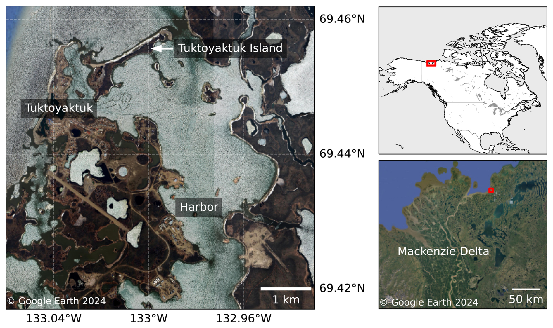
Figure 1 Overview map of the research area. Tuktoyaktuk Island is located close to the hamlet of Tuktoyaktuk, east of the Mackenzie Delta in northwestern Canada. The barrier island protects the harbor from incoming storms and waves.

Since the onset of Arctic amplification in 1970, air temperatures in the region are rising twice as fast as the global average (Hansen et al., 2010; Lenssen et al., 2019): 0.052 °C yr⁻¹ on average in the past 50 years to a current mean annual temperature of −8 °C (Lenssen et al., 2019; Lapham et al., 2020; GRID-Arendal, 2020). Rising temperatures lead to an extension of the open water period, enhancing thermoerosion: the permafrost-cemented cliffs are exposed to the heat transfer and mechanical abrasion from waves during a longer period of time, which accelerates permafrost thaw and thus coastal retreat (Berry et al., 2021). The coastal retreat rate at the island and the area of Tuktoyaktuk has been recorded since 1947 by the Geological Survey of Canada (GSC) using aerial photography, remote sensing and ground-based GPS surveys (Hynes et al., 2014). The northwestern coastline retreats particularly rapidly, at rates that have risen from 1.58 ± 0.05 to 1.80 ± 0.02 m yr⁻¹ in the past 20 years (Whalen et al., 2022). The southeastern coastline retreats much slower, but rates have also increased in the 21st century to 0.48 ± 0.04 m yr⁻¹ currently. Considering that the island measured only 36 m across at the narrowest point in 2022 and around 50 m over most of its stretch, Whalen et al. (2022) predict that it will be breached at the latest by the year 2044.

This will have severe consequences for the harbor of Tuktoyaktuk: it will be exposed to incoming storms as the most significant storms are from the N and NW (Manson and Solomon, 2007; Kokelj et al., 2012). The harbor has a traditional and economic importance to the community and to shipping, providing a basis for transportation and supply for other communities in the Inuvialuit Settlement Region, as well as an operating base for the Canadian Coast Guard. Numerous shore protection measures have been used to mitigate coastal erosion along the shoreface of the community starting in the 1970s, such as concrete blocks to fill up space left by thaw subsidence or geotextiles to protect the sediment from mobilization via the incoming waves, but all were damaged within a couple of years (Baird, 2019a). Currently, armorstone is still in place at several locations along the coast but does not prevent coastal retreat. A more recent study suggests mitigation of coastal erosion at the hamlet and at Tuktoyaktuk Island with sand reservoirs (Baird, 2019b).

2.2 Study design

In September 2021, we collected more than 30 marine ERT profiles around Tuktoyaktuk Island, oriented roughly parallel or perpendicular to the shoreline. Each profile consisted of numerous (tens to several hundred, depending on the length of the profile) adjacent vertical electrical soundings (VESs) in a quasi-symmetric reciprocal Wenner–Schlumberger array. The reciprocal array can result in a lower signal-to-noise ratio because the potential electrodes are located outside the innermost pair of current electrodes (Parsekian et al., 2017; Prins et al., 2019). However, the reciprocal array is suitable for the survey design as it allows for simultaneous measurements during the current injection (Fediuk et al., 2020). We used a floating multicore cable towed behind a boat at around 7 km h⁻¹ to collect the soundings at a spacing of around 5 m. The measurements were recorded with an IRIS Syscal Pro Deep Marine™ as a control unit, together with the IRIS Sysmar™ software on a connected field laptop. The IRIS Syscal Pro Deep Marine™ is designed to employ VESs with 13 electrodes (2 injection electrodes and 11 potential electrodes, measured simultaneously on 10 channels). We used a custom-made cable with 22 electrodes (leaving 9 electrodes unused). This allowed for various electrode configurations and achieved greater penetration depth due to its increased length compared to the standard 13-electrode cable. In the electrode configuration used, the 13 electrodes combine to 10 roughly vertically stacked soundings with a quasi-common center but different pseudo-depths (Fig. 2). Current was injected in the center of the cable with 10 m separation between the injection electrodes. The potential electrode pairs outside of the injection electrodes were separated by 15 to 115 m. The positions of electrode pairs at intermediate separations were slightly changed between the two days of acquisition. The GPS positions of the boat and at the center and tail of the cable were continuously recorded. The water depth was measured from the boat using an echosounder and later assigned to each sounding based on the coordinates of the cable center. In addition, water conductivity and temperature profiles were measured next to and in between some of the ERT profiles using either a SonTek CastAway™ or an AML Oceanographic™ CTD (conductivity–temperature–depth) instrument.

Assessment of the terrestrial and nearshore geology and of the nearshore bathymetry benefited from previous studies led by the Geological Survey of Canada (Boike and Dallimore, 2019), and completion of two terrestrial boreholes on Tuktoyaktuk Island and two nearshore boreholes was conducted in 2018 (Boike and Dallimore, 2019; Lapham et al., 2020).

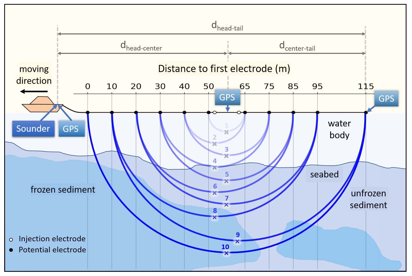
Figure 2 Marine ERT survey setup with floating electrodes. The potential electrode pairs have a quasi-common center but different pseudo-depths (depth of highest sensitivity, marked as “x”), thus forming VESs. GPS units were mounted on the boat (head), between the injection electrodes (center) and at the last potential electrode (tail), respectively, to assess the cable curvature based on the distances between the GPS units.

2.3 Analysis

The goal of the data analysis was to invert the ERT data to get a set of intersecting 2D resistivity models that could be used to determine the depth to the IBPT. We used the IBPT depth in combination with historical coastline data (Hynes et al., 2014) to estimate the resulting vertical permafrost degradation rate.

Before inverting the data, soundings with incorrect apparent resistivities needed to be removed. In a mobile marine survey electrode positions can potentially vary as the cable is flexible. A curved cable can lead to a change in the geometric factor and thus incorrect apparent resistivities as they are linearly dependent. Therefore, we quantified the curvature of the cable during the field measurements using the GPS data from the boat (“head”) and the center and tail of the cable. For a straight cable, the sum of the two segments “head–center” and “center–tail” is equal to the length “head–tail”. The difference between those distances $d_{\mathrm{d}}=d_{\text{head-center}}+d_{\text{center-tail}}-d_{\text{head-tail}}$ increases with increasing curvature. Under the simplest assumption of a circular bend, electrode positions along the curved cable could be determined for different values of d_d. Based on the modified electrode positions, the modified geometric factor k was calculated for every potential electrode pair (cf. Loke, 2001), considering the electrode positions and cable distortions in the horizontal plane. Taking into account the deviation of k for different degrees of curvature as well as the actual GPS data from the field, we derived a curvature (d_d) threshold above which measurements should be regarded as incorrect. Those soundings were excluded from the dataset. Where the exclusion led to data gaps in the profiles, the profiles were truncated into individual sections.

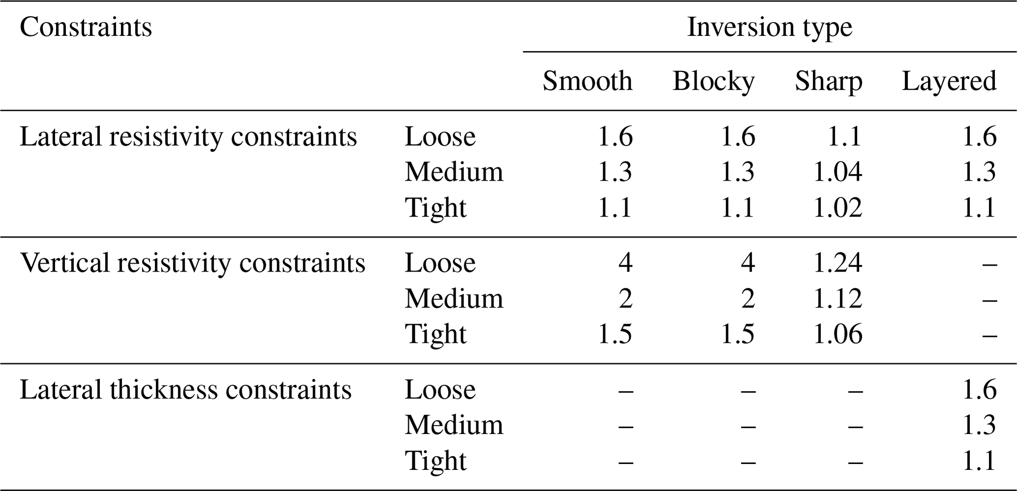
Every section in the filtered dataset was then inverted in 1D with lateral constraints (laterally constrained inversion, LCI) using Aarhus Workbench™ to construct 2D resistivity models (cf. Auken et al., 2005). Aarhus Workbench™ offers four inversion types: smooth, blocky, sharp and layered. The different inversion types have different penalizing parameters regarding the minimization of the lateral and vertical resistivity contrast between cells and thus result in models with different degrees of sharpness. The inversion can be refined for each inversion type by varying lateral and vertical resistivity constraints, i.e., by defining a maximum standard deviation of the resistivity contrasts between neighboring cells (Table 1). We followed the recommendations in the manual by varying the lateral and vertical resistivity constraints between the default values for loose, medium and tight constraints. The water layer resistivity was set to a starting value based on the CTD measurement closest to the profile and taken on the same day as the ERT, and its variation was constrained during inversion. The depth of investigation (DOI) was calculated internally during the inversion according to Vest Christiansen and Auken (2012) using a default sensitivity threshold of 0.75.

Goodness of fit between the forward response and the measured data was estimated using the data residual, a metric used by the inversion software Aarhus Workbench™. It can be regarded as the root mean square (RMS) weighted with the standard deviation (noise level) of the measurement. A data residual close to 1 indicates a good fit between the resistivity and the noise level of the model and the data. As we only roughly estimated the noise level (at 10 %), the data residual should be considered an error estimate for comparison between different profiles and not an exact measure for underfitting (data residual of > 1) or overfitting (data residual of < 1). The data residual and the RMS were calculated with the resistivity in logarithmic space.

Table 1 Default constraints for the different inversion types available in Aarhus Workbench™. The vertical constraints should always be looser than the lateral constraints for the representation of a layered medium. The discretization implies that the layered model has no vertical resistivity constraints and that the other three models have no lateral thickness constraints.

To provide a basis for comparison of the results from the four inversion types, we tested combinations of inversion types and constraints on a synthetic model to determine the most suited inversion technique for the specific setting. The synthetic model was set up in pyGIMLi (Rücker et al., 2017) and based on information on the local permafrost conditions from two technical reports that contain exemplary IBPT depths below the seabed and electrical resistivities of the terrestrial permafrost (Boike and Dallimore, 2019; Baird, 2020). The synthetic model consisted of three layers representing the water column, the unfrozen sediment and the frozen sediment, respectively (Fig. 3). Resistivities were constant throughout the layers at 6.1, 10 and 1000 Ω m. The water layer resistivity was based on field measurements, whereas the sediment resistivities were chosen based on Overduin et al. (2012). The water layer had a depth of around 5 m, and the interface between the second and third layer slightly dipped at varying angles. Through a forward operation following the survey design used in the field, ERT data were simulated that subsequently could be inverted in Aarhus Workbench™.

Figure 3 Synthetic model used to infer the most suited inversion technique for this specific setting. The model consists of three layers: the upper layer represents the waterbody with a depth of 5 m and a resistivity of 6.1 Ω m. The second and third layers have resistivities of 10 and 1000 Ω m, representing unfrozen and frozen sediment, respectively. The boundary between the two layers ranges from depths of 7 to 30 m and dips at varying angles, which is a plausible scenario for the IBPT in a profile perpendicular to the shoreline of Tuktoyaktuk Island.

In addition to testing four inversion types, we tested three approaches to determine the interface between unfrozen and frozen sediment (i.e., the IBPT depth): (1) a fixed resistivity range in which the transition from unfrozen to frozen is assumed to occur, in line with previous studies (Fortier et al., 1994; Overduin et al., 2012, 2016), (2) the highest vertical resistivity gradient in linear space and (3) the highest vertical resistivity gradient in logarithmic space. Those criteria were applied to the resistivity models obtained from the inversion of the simulated data. The combination of the inversion type, constraints and IBPT determination approach that resulted in the smallest offset between the estimated IBPT and the synthetic-model IBPT was assessed to provide the most accurate estimated IBPT depth and therefore applied to the entire dataset. We distinguished between the following terms:

• estimated IBPT, which is the depth of the highest vertical resistivity contrast in the inversion result (in linear or logarithmic space), and

• synthetic-model IBPT, which is the fixed boundary between the second and third layer in our synthetic model, representing the IBPT.

To quantify the offset, we used the RMS of the difference along each column of the inversion grid, aiming to put a stronger weight on columns with a greater offset between the estimated IBPT and the synthetic-model IBPT. RMS values for this offset are given in units of meters. Although centimeter scale values for this derived value are retained for comparison between profiles, this does not imply centimeter scale accuracy in IBPT depth estimates.

We used historical coastline data to estimate the time since inundation along our profiles. The coastlines were digitized from 19 aerial photographs taken between 1947 and 2001 and combined with more recent GPS measurements and satellite imagery. The data were first presented by Solomon (2005) and later compiled for geographic information system (GIS) application by Hynes et al. (2014). Since the vast majority of our profiles lines lay outside of the 1947 coastline, we extrapolated the time since inundation linearly to every sounding coordinate (with a mean coastal retreat rate of 2 m yr⁻¹). Along with the IBPT depth from our ERT surveys we used the time since inundation to estimate the average vertical permafrost degradation rate through linear regression.

3 Results

3.1 Inversion and IBPT depth

3.1.1 Analysis and calibration with synthetic data

We tested smooth, blocky, sharp and layered LCIs with varying lateral and vertical resistivity constraints (varying lateral resistivity and lateral thickness constraints in the layered inversion; see Table 1) on simulated ERT data from a synthetic model. The inverted models for medium lateral resistivity constraints and medium vertical resistivity (or lateral thickness) constraints are shown in Fig. 4 and illustrate the differences between the inversion types. The smooth inversion produced a model with a constant or only slightly varying resistivity gradient, which makes the determination of the highest vertical resistivity gradient ambiguous. In contrast, the layered model provides a defined boundary between the unfrozen and frozen layer. However, the resistivity and thickness of the unfrozen layer were strongly correlated, producing unrealistic models for most of the constraint combinations. The blocky and sharp inversions represent compromises between the smooth and layered inversion. Blocky inversions tended to show resistivity variations within the frozen layer, while sharp inversion models exhibited fewer variations within the layers but often displayed strong artifacts at the seabed boundary.

Comparing the different approaches to determine the IBPT from a given inversion as described in Sect. 2.3, we found that, overall, the IBPT depths calculated in logarithmic space were up to 10 times closer to the synthetic-model IBPT than the ones calculated in linear space. In only 5 out of 27 of the tested combinations was the estimated IBPT in linear space closer to the synthetic-model IBPT (up to 15 %). In addition, the IBPT calculated in the linear space lay mostly well below the DOI (>10 m deeper). In contrast, the IBPT calculated in logarithmic space lay mostly above the DOI and locally only one or maximum two cells below the DOI. The comparison between linear and logarithmic IBPT applies to the smooth, blocky and sharp inversions; in the layered inversions both are the same.

We imposed additional criteria on determinations of the IBPT, mostly to exclude false positives: (1) the IBPT depth had to exceed the water depth, as we expect unfrozen sediment on top of the IBP; (2) the resistivity below the IBPT had to exceed 10 Ω m, with a lower resistivity being assumed to correspond to unfrozen sediment (cf. Overduin et al., 2012); and (3) the median gradient for every model had to exceed 0.02 Ω m m⁻¹. This last criterion was determined empirically and applied to exclude inversions with only a subtle peak in the resistivity gradient that would not be a reliable indicator for the IBPT.

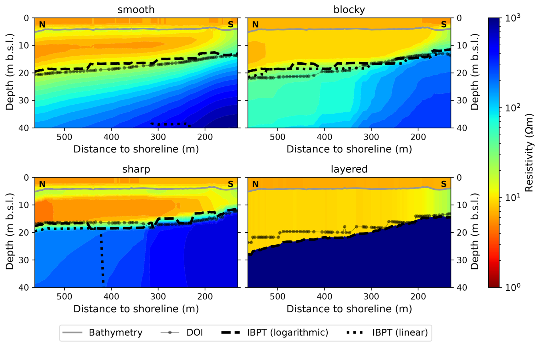
Figure 4 Comparison between the smooth, blocky, sharp and layered inversions (with medium lateral resistivity and medium vertical resistivity/lateral thickness constraints) of the simulated ERT data from the synthetic model. The models show different transitions between the second and the third layer (representing unfrozen and frozen sediment in Fig. 3). The inferred IBPT, identified as the highest vertical resistivity gradient in logarithmic space, is close to the DOI in all four models. The blocky model's inferred IBPT is closest to the actual boundary in the synthetic model.

A blocky inversion with tight lateral and medium vertical constraints and the corresponding IBPT calculated in logarithmic space respecting the criteria described above most precisely identified the IBPT in the synthetic model. The RMS of the offset between the inferred IBPT from the inversion and synthetic-model IBPT for this inversion type was 2.76 m. The estimated IBPT matched the synthetic-model IBPT to a precision below one grid cell size (2 m at 20 m depth); only towards the rim the offset was larger. A blocky inversion with tight lateral and tight vertical constraints and a sharp inversion with tight lateral and medium vertical constraints showed a similar performance (RMS offset of 2.80 and 3.08 m, respectively). The layered inversions were neglected in the comparison as they produced lower RMS offset values but unrealistic resistivity distributions (correlated electrical resistivity and water depth). For all inversion types, the data residual increased with tightening constraints but was only used as a secondary quality indicator as the noise level of the measurement cannot be determined and was therefore estimated to be 10 % for the calculation of the data residual. If only individual data points showed an extremely high residual, they were removed before re-running the inversion. This reduced the effect of the outliers on the inversion result and lowered the data residual.

3.1.2 Analysis of field data

The LCIs of field data are shown in Fig. 5 for a selection of profiles around Tuktoyaktuk Island. In each tomogram, the IBPT calculated in linear and logarithmic space was compared to the DOI. Gray dots represent the data points of the inversion and show the cell thickness. The water layer in each model was constrained by the CTD measurements taken closest to the profiles on the day of the ERT surveying. As the water column showed no stratification, the water resistivity of the model was constrained uniformly throughout the layer.

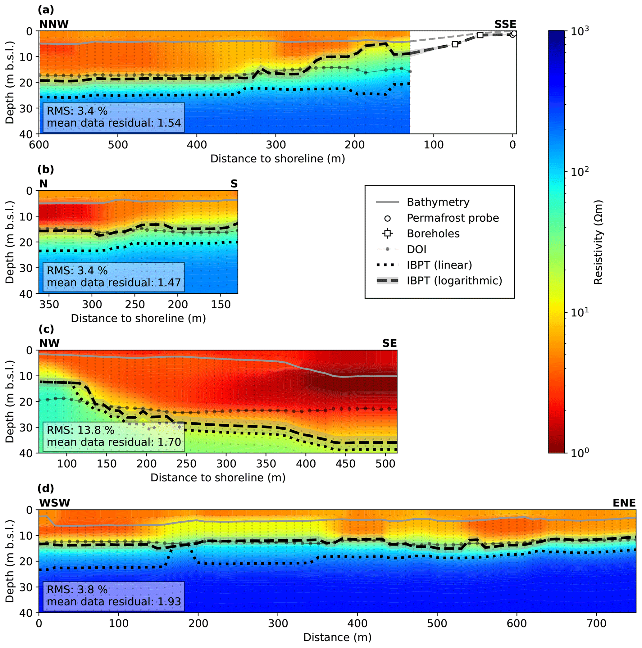
Figure 5 Comparison of IBPT calculations (linear and logarithmic) and DOI across selected inverted resistivity models. The locations of the selected profiles are indicated in Fig. 6. (a) The profile was located north of the island, perpendicular to the shoreline. The IBPT dipped towards the offshore part, where it remained constant for several hundred meters. Towards the shore, the IBPT was extended based on borehole information (Boike and Dallimore, 2019) and permafrost probe measurements. (b) The profile lay perpendicular to the northern shoreline, east of the profile in (a). The dipping of the IBPT from S to N was not as pronounced as for the profile shown in (a). (c) The profile lay south of Tuktoyaktuk Island and extended from NW (close to the coast) to SE (towards the harbor basin). The IBPT dipped steeply and lay deeper compared to the other profiles; however, the section lying several grid cells below the DOI should be treated with caution. (d) The profile ran parallel to the northern shoreline at around 15 m from the shore. The IBPT was mostly horizontal.

The profile corresponding to Fig. 5a lay north of the island and extended from the NNW to SSE. The IBPT inferred from the model was extended based on borehole information (Boike and Dallimore, 2019) and permafrost probe measurements conducted in September 2021. The water layer and the unfrozen sediment layer had a similar resistivity with slight variations that could be interpreted as compensation for a slight spatial variation in water resistivity. The transition from an unfrozen to a frozen layer (as identified by the highest logarithmic resistivity gradient) occurred between 10 and 50 Ω m, and the permafrost below showed resistivities of 50 Ω m to several hundred. The depth of the IBPT was shallow (5 to 10 m b.s.l.) at a distance up to 250 m from the shoreline and descended to a stable level around 20 m b.s.l. further offshore (250 to 600 m from the shore). The mean data residual was 1.54 (RMS = 3.4 %).

The profile corresponding to Fig. 5b lay perpendicular to the northern shoreline and extended from the N (offshore) to S (around 130 m from the coast). The water depth was around 4 to 5 m, and the IBPT was inferred at around 13 to 17 m b.s.l., close to the DOI. The dipping of the IBPT from the S to N was not as pronounced as for the profile shown in Fig. 5a but was rather at a constant depth below the slightly northwards dipping seafloor. The mean data residual was 1.47 (RMS = 3.4 %).

The profile corresponding to Fig. 5c lay south of Tuktoyaktuk Island and extended from the NW (close to the coast) to SE (towards the harbor basin). The water depth ranged from 2 m close to the coast to around 10 m. In the deep water, the resistivity below and slightly above the seabed was very low (below 1 Ω m), which could be an artifact compensating for changes in the resistivity of the deeper water. The IBPT ranged from 12 m b.s.l. close to the coast to around 35 m b.s.l. where the water was deeper. A significant stretch of the IBPT lay several meters below the DOI, where the sensitivity was very low and the IBPT depth should be treated with caution. However, we expected a deeper IBPT south of Tuktoyaktuk Island due to deeper water and slower coastal retreat rates that imply longer inundation times at similar distances from the coast and thus a longer period of subsea permafrost degradation. The mean data residual was 1.70 (RMS = 13.8 %).

The profile corresponding to Fig. 5d lay parallel to the northern shoreline and extended from the WNW to ENE at around 150 m from the shore. The water depth varied between 3 and 7 m, and the IBPT was inferred to be mostly horizontal between 12 and 16 m b.s.l. close to the DOI. The resistivity ranges were similar to the profile in Fig. 5a. The mean data residual was 1.93 (RMS = 3.8 %).

A blocky inversion with tight lateral and medium vertical constraints was applied to the whole dataset. Inferred IBPT depths are represented in Fig. 6. It appears that the IBPT depth ranged from 5 to 25 m b.s.l. north of the island at water depths from below 5 to over 20 m. The historical coastlines show that the northern shore facing the open ocean is subject to faster coastal erosion than the southern side. The profiles were mostly located outside the historical coastlines as the water was too shallow closer to the coast to be reached with the boat. Therefore, the borehole locations were not crossed by the ERT surveys. South of the island, the IBPT ranged from 10 to 30 m b.s.l. at water depths from 10 to over 35 m. Several profiles were removed south of the island (shaded lines) as they did not return reasonable IBPT depths (i.e., depths well below the DOI; see Discussion). Intersections between profiles were thus only found north of the island. They can be used to validate our IBPT determination method. Most intersections showed a difference in the IBPT depth below 10 %, which corresponds to a deviation of zero or one grid cell of the inversion and depending on the depth to an absolute deviation of up to 2 m. However, a few intersections showed differences in the 15 %–20 % range (two grid cells or up to 4 m), and one intersection even deviated by 35 %. These percentages are of course dependent on the grid size used in the inversion, and the distribution would be more scattered for a finer grid. The raw apparent resistivities at the intersections matched very well (average deviation of 0.9 ± 1.2 Ω m), which means that the measurement was not dependent on the orientation of the profiles. Deviations in the IBPT at the intersections therefore most probably originated from lateral constraints.

Figure 6 (a) Map view of the IBPT depth around Tuktoyaktuk Island. The red arrows indicate the directions of the highlighted profiles of Fig. 5a–d. South of the island, several profiles have been removed (transparent lines). The historical coastlines since 1947 show the faster degradation of the northern shoreline facing the open ocean (Hynes et al., 2014). Most of the profiles however lay beyond the shoreline of 1947. Boreholes from Boike and Dallimore (2019). (b) IBPT depth over the distance to the shore, south and north of Tuktoyaktuk Island. The remaining profiles south of the island indicated a steeper slope of the IBPT compared to the northern side. The profiles shown in Fig. 5 are highlighted in red.

The vertical subsea permafrost degradation rate was estimated north of the island under the assumption of a constant coastal retreat rate within the past 270 years. The IBPT depth used for the calculation was taken from the representative profile shown in Fig. 5a. At 20 m depth (approximate depth of the IBPT from 350 to 550 m offshore), the cell thickness was around 2 m, which lead to an even lower resolution at that depth and was also the reason for small but abrupt step-like changes in the IBPT depth within only a few meters in the lateral direction. The uncertainties in the IBPT depth due to an inversion resolution thus ranged from ±0.5 to ±1 m (half the layer thickness). The inundation time was extrapolated from historical coastline data. According to a linear regression, the vertical subsea permafrost degradation rate was 5.3 ± 4.0 cm yr⁻¹.

3.2 Geometry

3.2.1 Geometric factor variation

Marine electrical resistivity surveys using a floating cable towed behind a boat can introduce uncertainties in the positions of the electrodes. Because the cable is flexible, it may curve depending on conditions such as the boat's path, wind or currents. This curvature leads to two sources of uncertainty: (1) a deviation in the geometric factor compared to a straight cable, due to changes in the relative distances between the electrodes, and (2) a lateral deviation of the cable center (Fig. 7). It appears that for a perfectly circularly bent cable, the relative change in the geometric factor $k/k_{\mathrm{straight}}$ is proportional to the distance difference d_d (Fig. 7b). The rate of change increases with electrode spacing; i.e., the inner electrodes pairs deviate less than the outer electrode pairs. The deviation for a circular bend remains relatively small for all electrode pairs. Even for relatively high degrees of curvature (corresponding to d_d=3 m), k is only increased by 7 ‰ for the outermost electrode pair. For an irregularly bent cable, the ratios of the distances between electrodes can be expected to change to a greater degree and have a larger effect on the geometric factor. For example, the geometric factor variation is larger if the cable is only partly curved, as the electrode positions are no longer symmetrical and the ratios between the distances considered in the calculation of the geometric factor are disturbed. Although simulations showed that it is possible to have only a slight or even no variation in k with an asymmetrically bent cable (for very specific configurations) the deviation is most often larger. It is therefore not possible to choose a universal threshold for the deviation of k below which the soundings can be considered acceptable and to filter the data according to the corresponding distance difference. Instead, a distance difference threshold must be set empirically and by considering the second source of uncertainty as well.

3.2.2 Lateral deviation

The second source of uncertainty in a mobile marine survey is the lateral deviation of the cable center from the GPS-recorded boat path (Fig. 7c). The sensitivity of the electrode array is predominantly concentrated below the injection electrodes at the cable center. Therefore, a survey with a curved cable risks mapping a slightly different sounding location, where the boat path deviates from that of the cable center.

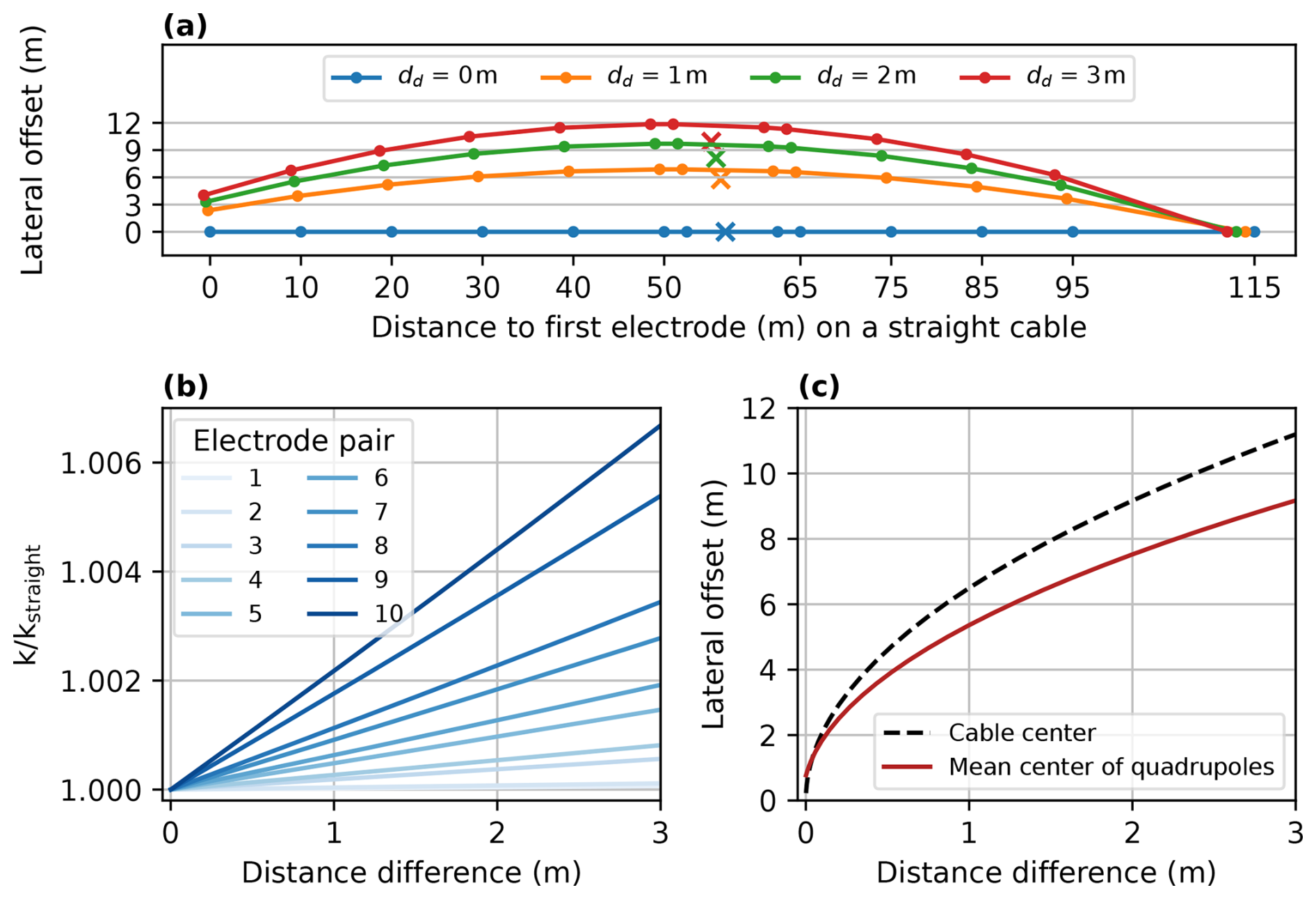
Figure 7 Sources of uncertainty arising from a curved cable. (a) Top view of curved-cable configurations. The dots represent the electrode positions along the cable for different degrees of curvature, and the crosses mark the corresponding highest-sensitivity area for a VES (i.e., the mean center of the 10 quadrupoles). (b) Relative change in the geometric factor depending on the distance difference for the 10 potential electrode pairs. (c) Lateral offset of the cable center and the mean center of quadrupoles depending on the distance difference.

Considering these two theoretical sources of error, we evaluated the performance of different d_d thresholds and found that a threshold of 1 m eliminated strongly curved parts of the profiles where both a lateral deviation of the cable center and a deviation of the true geometric factor were highly probable. Therefore soundings with d_d>1 m were removed from the dataset and not inverted. During part of the acquisition, the center GPS did not record. In this case, we used only the distance from the head to the tail as a curvature criterion. We applied a threshold of 125.7 m as a minimum distance between the head and the tail, which corresponds to the (mean) head-to-tail distance of the measurements with d_d=1 m. For some profiles the head-to-tail distance was slightly lower but constant. For those profiles we tolerated soundings with a head-to-tail distance of >125.0 m.

4 Discussion

4.1 Inversion

Our inversions showed a relatively high data residual throughout all four inversion types compared to similar studies (e.g., Angelopoulos et al., 2021). However the data residuals are relative values and cannot be used to evaluate the quality of the inversion since the ambient noise level of our measurements is unknown. In order to use the data residual for the comparison and assessment of the different inversion types, repeated measurements (e.g., by anchoring the boat and fixing the cable at the shore or using a second boat) would be needed to estimate the noise level. However the data residual still indicates the relative fit between data points of one model and is often unevenly distributed. This could be explained by slight spatial variations in water salinity or temperature, i.e., water resistivity (with salinity being the far more dominant factor since temperature changes were only minor). As the water makes up a large portion of the sensitivity area and the layer is constrained in the inversion, it might be difficult to fit the model to possibly inaccurate water resistivities. Arboleda-Zapata et al. (2022) showed how sensitively the inversion reacts to the water layer resistivity and thus how important it is to constrain the inversion based on a dense net of CTD measurements. In the case that the water layer is stratified it might even be useful to incorporate two water layers in the inversion, but our CTD measurements indicated a homogeneous water layer.

Although the data residual could not be used to compare the different inversion types and parameterizations, we were able to determine a best-suited inversion type for the specific application using a synthetic model. A three-layer model with constant resistivities is without a doubt oversimplified but is close enough to the real setting to evaluate the performance of the inversion types in the given setting. We evaluated whether the resistivity distribution obtained in the inversion of the simulated data reflected the (synthetic) IBPT by the highest gradient of the logarithmic resistivities. This approach led to a best-suited inversion type. This evaluation of inversion types is only valid for our specific case, but the approach could potentially be adopted in other studies.

We found that the IBPT was best represented using a blocky inversion with tight lateral and medium vertical constraints and by calculating the highest resistivity gradient in logarithmic space. A blocky inversion with tight lateral and tight vertical constraints performs almost equally well, so it was also tested on the field data and returned very similar IBPT depths. The IBPT is often close to the DOI, sometimes slightly below. This can be expected and does not refute our interpretation because the electric field is expected not to penetrate deep into the IBP due to its high resistivity so that the DOI is near the interface from unfrozen to frozen ground. This also implies that the actual resistivities of the IBP are not reliable and must be seen only as a contrast to the overlying lower resistivities. The potential ambiguity of the peak in the resistivity gradient is also important to consider. Especially in the smooth inversion, there are often multiple peaks along the vertical resistivity gradient so that there is no clear indication of the IBPT depth. In the blocky and sharp inversion, this problem does not occur and the peaks are always unique. Nonetheless, it is important to implement additional criteria to avoid undesired IBPT picks, such as the water–seabed interface being identified as the IBPT; IBP being suspected in areas of low resistivities; or a maximum gradient being picked, although there is no big vertical contrast over the whole depth of the model. We addressed this issue by setting a minimum depth (i.e., z_IBPT>z_water), a minimum resistivity (10 Ω m) and a minimum resistivity gradient (median of 0.02 Ω m m⁻¹ over the entire model). The latter serves to avoid finding boundaries in a homogeneous resistivity distribution and was set empirically. Especially for several profiles south of the island with water depths up to 18 m, the penetration depth of the applied measurement configuration is not sufficient to penetrate the sediment deeply enough to identify the IBPT. Therefore, the area above the DOI is homogeneous in resistivity (only water) and the automatically detected IBPT lies well below the DOI, where the inverted model is able to create greater resistivity contrasts without changing the forward operation. These profiles were neglected in the analysis.

When discussing uncertainties of the reconstructed depth of the IBPT, not only plausible alternative models but also the uncertainties of the “best-suited” model itself are important to consider. Due to the discretization using 30 cells with logarithmically increasing thickness below the seabed, the vertical spatial resolution of each model decreases with depth. The water layer thickness uncertainty is given by the resolution of the bathymetric measurements at an estimated uncertainty of 10 cm. The cell thickness of the first layer below the water layer is 1 m. Features that are smaller than the cell size cannot be resolved by the inversion. Our permafrost probe measurements at the shore revealed IBP depths greater than 1 m (which corresponds to the order of subaquatic active layer depths; Osterkamp et al., 1989).

But there is the potential to obtain a more precise IBPT depth. Besides a finer grid in the inversion, additional measurements in the field could help to reduce the non-uniqueness of the inversion. A more dense net of water resistivity measurements would be helpful, and Arboleda-Zapata et al. (2022) suggested that sampling of the sediment to narrow down its electrical resistivity and optimizing the electrode array for detection and characterization of permafrost layers may help to identify the boundary between frozen and unfrozen ground more precisely. Furthermore, the comparison with borehole data would be very valuable. Unfortunately, the boreholes available on the northern shore of Tuktoyaktuk are located in shallow water and were not reachable with the boat during our campaign in 2021. Future surveys may include measurements where the end of the cable is manually pulled towards the shore so that shallow parts can be covered, while the boat stays in deeper water.

In addition to marine ERT, other geophysical methods are able to detect the IBPT depth in subaquatic environments (Angelopoulos et al., 2020). Reflection and refraction seismic methods have been widely used, especially in deeper waters (Brothers et al., 2012), but often demand higher logistical costs. An alternative and easily deployable method for shallow coastal areas relying on seismic signals has been presented by Overduin et al. (2015), who use ambient noise to detect subsea permafrost. Ground-penetrating radar can be effective in non-saline water areas for mapping frozen sediment, especially in bedfast ice zones (Stevens et al., 2009). Transient and controlled source electromagnetic surveys have also proven to be useful in offshore environments (Koshurnikov et al., 2016; Sherman and Constable, 2018). Besides the presented inversion approaches, global ERT inversions have been shown to retrieve good results at estimating IBPT depths (Arboleda-Zapata et al., 2022). Identification of the IBPT independent of sediment and porewater characteristics, however, generally requires direct observation through drilling (Angelopoulos et al., 2020).

4.2 Permafrost degradation

We observed two distinct permafrost settings north and south of Tuktoyaktuk Island, each of which is explained by a different landscape evolution. North of the island, marine transgression led to an inundation and warming of continuous permafrost, resulting in degradation. The mean annual permafrost degradation rate decreases with increasing distance from the coastline (and thus greater inundation times) due to a weakening of the chemical and thermal gradient with increasing IBPT depth (Angelopoulos et al., 2019; Hutter and Straughan, 1997, 1999). The degradation rates calculated from the IBPT depths over the inundation times of the boreholes are 10.2 and 6.6 ± 3.0 cm yr⁻¹, respectively, thus also indicating faster degradation closer to the shore. However, the calculated degradation rate and its uncertainty range must be treated with caution as we are neglecting the error in inundation time induced by varying coastal erosion rates within approximately the past 270 years.

The sharpness of the transition from ice-free sediment to IBP over depth is unlikely to be the same everywhere. Certain sediment and porewater conditions facilitate a gradual transition: (1) clayey permafrost with high unfrozen water content; (2) pre-existing cryopeg prior to inundation; and (3) any environment in which salt diffusion keeps pace with heat diffusion, i.e., a subsea setting with significant convection. In any case, a long inundation period is generally required for a gradual transition to develop and is unlikely in such a coastal setting. The two borehole logs showed a sharp transition on the sub-centimeter spatial scale (Boike and Dallimore, 2019).

South of Tuktoyaktuk Island, the setting was different and the IBPT dipped more steeply than on the northern side, to depths of over 20 m b.s.l. at less than 100 m from the coast. At these depths, the sensitivity of the geoelectrical measurements is drastically reduced (Sellmann et al., 1989; Arboleda-Zapata et al., 2022). More advanced degradation is expected as the southern shoreline currently retreats at least 4 times more slowly than the northern shoreline, which implies longer inundation times at similar distances from the shore. However, a very deep IBPT or even the absence of IBP within the depth of investigation of the ERT might also be the result of taliks that were present prior to marine submergence. Such taliks would have existed below thermokarst lakes or river channels associated with the former outlet that shaped the Tuktoyaktuk harbor basin. Our bathymetric records locally showed water depths exceeding 20 m to the south of Tuktoyaktuk Island, which may be the result of dredging, the pre-inundation thermokarst lake floor position, seafloor subsidence following permafrost thaw or some combination of these.

The comparison between the data presented here from Tuktoyaktuk Island and other data from the Beaufort Sea showed that the IBPT at Tuktoyaktuk was a few meters deeper (for the same inundation time) than at other locations for which comparable data are available (Harding-Lawson-Associates, 1979; Osterkamp et al., 1989; Taylor et al., 1996; Angelopoulos et al., 2020). In the Alaskan Beaufort Sea, e.g., the IBPT was at least twice as deep as on the Canadian Shelf close to the Mackenzie Delta (Harding-Lawson-Associates, 1979). This also applies to inundation times of several thousands of years (Harding-Lawson-Associates, 1979; Osterkamp et al., 1989). As first explained by Harrison and Osterkamp (1978), the coarse sediments of the Canadian Beaufort Shelf could facilitate density-driven salt flow to the phase boundary, thereby enhancing salt diffusion at the IBPT and degradation of the IBPT. However, the discharge of the Mackenzie Delta is likely to be the dominant factor influencing the relatively rapid IBPT degradation. The year-round freshwater input can lead to particularly warm mean annual bottom temperatures (especially in shallow waters with <10 m depth), accelerating subsea permafrost degradation (Taylor et al., 2013). A similar effect has been observed at Muostakh Island, influenced by the Lena River discharge (Overduin et al., 2016; Shakhova et al., 2017).

4.3 Geometry

Our GPS data showed that the distance difference d_d is a reliable indicator for the degree of cable curvature, especially for slight curvatures. From our geometric considerations it is however not possible to quantify the exact deviation of the geometric factor resulting from the shifted electrode positions because the bent cable may have an asymmetric curvature rather than form a circular arc. However, even for an asymmetric curvature, soundings with d_d<1 m were only affected negligibly by a deviating geometric factor. To further elaborate the approach of quantifying the cable curvature and the exact deviation of the geometric factor, precise knowledge of all electrode positions would be needed. Given the exact positions, even soundings with a strongly curved cable could be corrected and still used in further analysis, increasing the amount of available data, especially in areas where extended straight boat paths may be unrealistic due to the local geography. During a small test campaign, we tested the use of GPS units at every electrode, but the accuracy of the devices was disturbed and thus not sufficient for exact positioning. Improved GPS accuracy would be desirable in future surveys as exact electrode positioning in marine surveys is very valuable. Other possibilities for reducing the error induced by a curved cable include directly controlling the cable straightness by making use of a second boat on the tail of the cable or using rigid supporting material along the cable.

5 Conclusions

In our study we presented the use of marine electrical resistivity data to estimate the depth to the IBPT at Tuktoyaktuk Island, a natural permafrost-stabilized barrier that protects the harbor of the hamlet of Tuktoyaktuk. We illustrated a possible analysis strategy that accounts for potential inaccuracies arising from the survey design, ambiguities of different inversion types and the difficulty in inferring the IBPT from a resistivity model.

Our findings indicated a slowly dipping IBPT north of Tuktoyaktuk Island that is consistent with the relatively fast coastal erosion rate there. In contrast, south of the island, where the coastal erosion is significantly slower, the IBPT dipped more steeply. Based on the historical coastal retreat rates, we inferred a mean vertical permafrost degradation rate north of the island of 5.3 ± 4.0 cm yr⁻¹.

We highlighted the potential of marine geoelectric surveys as well as the difficulties and possible measures for further improvement in both fieldwork and data analysis in order to narrow down the uncertainty of IBPT depths. Our filtering approach allowed us to rely on soundings with a minimal positional error in the inversion. We addressed the ambiguity of different LCI parameterizations by testing them on a representative synthetic model and presented approaches for simplifying data processing and interpretation for future field campaigns. Precise electrode positioning or more frequent CTD measurements, for example, promise to increase the reliability of the inversion and thus to make its interpretation easier.