Physically based modelling of glacier evolution under climate change in the tropical Andes

In recent years, opportunities have opened up to develop and validate glacier models in regions that have previously been infeasible due to observation and/or computational constraints thanks to the availability of globally capable glacier evolution modelling codes and spatially extensive geodetic validation data. The glaciers in the tropical Andes represent some of the least observed and modelled glaciers in the world, making their trajectories under climate change uncertain. Studies to date have typically adopted empirical models of the surface energy balance and ice flow to simulate glacier evolution under climate change, but these may miss important non-linearities in future glacier mass changes. We combine two globally capable modelling codes that provide a more physical representation of these processes:(i) the Joint UK Land Environment Simulator (JULES), which solves the full energy balance of snow and ice, and (ii) the Open Global Glacier Model (OGGM), which solves a flowline representation of the shallow-ice equation to simulate ice flow. JULES–OGGM is applied to over 500 tropical glaciers in the Vilcanota-Urubamba basin in Peru, home to more than 800 000 people that predominantly live in rural communities with low socioeconomic development and high vulnerability to climate change. The model is evaluated against available glaciological and geodetic mass balance observations to assess the potential for using the modelling workflow to simulate tropical glacier evolution over decadal timescales. We show that the JULES–OGGM model can be parameterized to capture decadal (2000–2018) mass changes in individual glaciers, but we also show that limitations in the JULES prognostic snow model prevent accurate replication of observed surface albedo fluctuations and mass changes across all glaciers simultaneously. Specifically, the model cannot replicate the feedbacks between the driving meteorology, surface energy balance, ablation processes, and snow darkening. Only by forcing the model with observed net radiation variables were we able to capture observed surface albedo dynamics. When driven with statistically downscaled climate change projections, the JULES–OGGM simulations indicate that, contrary to point-scale energy balance studies, sublimation plays a very minor role in glacier evolution at the basin scale and does not bring about significant non-linearities in the glacier response to climate warming. The ensemble mean simulation estimates that total glacier mass will decrease to 17 % and 6 % of that in 2000 by 2100 for Representative Concentration Pathway (RCP) 4.5 and RCP8.5, respectively, which is more conservative than estimates from some other global glacier models.

1 Introduction

Meltwater from tropical Andean glaciers buffers water supply to domestic users, agriculture, and energy supply during periods of drought (Buytaert et al., 2017; Carey et al., 2014; Ultee et al., 2022). The magnitude of buffering will be inhibited in the future as glaciers recede in a warming climate. Large-scale earth observation analyses of historical glacier extent and geodetic mass balance indicate that tropical Andean glaciers have been receding rapidly in recent decades. Dussaillant et al. (2019) found that between 2000 and 2018 the average mass balance of glaciers in the tropical Andes was −0.42 ± 0.24 m yr⁻¹ w.e. Seehaus et al. (2019) estimated that glacier extent in the Peruvian Andes, home to ∼ 70 % of the world's tropical glaciers, reduced by 29 % between 2000 and 2016, with over half of this retreat occurring in the last 3 years of this period. Taylor et al. (2022) estimated glacier area losses of between 54 % and 64 % (1970–2020) across three mountain ranges in the southern Peruvian Andes.

There is high confidence that temperatures in the Andes will continue to increase throughout the 21st century (IPCC, 2023; Yarleque et al., 2018). The diversity of meltwater end users and potential impacts of climate change necessitate reliable projections of glacier mass changes to inform policy and adaptation pathways (Johansen et al., 2018). This is especially true in the tropical Andes, where many aspects of future climate change remain highly uncertain due to inadequate climatic and glaciological monitoring networks.

Providing reliable projections of glacier mass changes for the tropical Andes is challenging, and this is due in part to the high spatiotemporal variability in ablation processes. At lower elevations below the equilibrium line altitude, ablation is dominated by melt. At higher elevations, point-scale energy balance studies show that sublimation can reduce the energy available for melting, particularly in the cooler dry season when humidity is low and the surface roughness of ice is higher (Gurgiser et al., 2013; Winkler et al., 2009). The implications of this for simulating glacier mass change were demonstrated by Fyffe et al. (2021). They applied an energy balance model at five on-ice meteorological stations in the Cordillera Blanca and Cordillera Vilcanota in Peru and perturbed precipitation and temperature inputs to explore the mechanisms of mass balance sensitivity to climate. They showed that at lower elevations the mass balance signal was driven by a switch from snow to rainfall. At higher elevations, the change in mass balance was driven by a switch from sublimation to melt processes. The mass balance response to climate warming should therefore be expected to be non-linear and spatially variable in response to temperature changes brought about by climate change. Indeed, Marzeion et al. (2012) concluded that the inability of their temperature index model to capture glacier mass dynamics in the tropics likely stemmed from the fact that it did not account for sublimation processes. Simulating mass changes over periods of decades is further complicated by the need to account for ice mass redistribution and the corresponding elevation feedback to accumulation and ablation processes (Huss et al., 2010; Van Tiel et al., 2018).

The sparsity of glacier monitoring data and meteorological observation networks in the tropics (Gärtner-Roer et al., 2019) has led many glacier evolution modelling studies to use simplified models that do not necessarily account for potentially important processes (e.g. Somers et al., 2019, did not explicitly model ice flow) or constrain their simulations to discrete on-ice locations where required observation data exist (Fyffe et al., 2021; Rabatel et al., 2013), limiting their usefulness for basin-scale assessments of meltwater perturbations under climate change. However, significant advances in methods to derive glacier mass variations from earth observation data has led to the development of regional and global geodetic datasets of glacier mass change in recent years (Dussaillant et al., 2019; Hugonnet et al., 2021). While they are subject to uncertainty, they provide the means to validate glacier evolution model simulations in regions that have previously been infeasible due to lack of field data. The availability of these data has coincided with the development of a growing number of large-scale (up to global) glacier evolution models (Marzeion et al., 2020). The Open Global Glacier Model (OGGM) is the first open-source “community” model for global glacier modelling (Maussion et al., 2019). It takes advantage of global glacier outline and topographic datasets, automated approaches for glacier geometry delineation, and global geodetic and glaciological mass balance data for parameter identification to provide a workflow through which users can build and run an ice dynamics model of any glacier in the world. The availability of flexible, globally capable glacier modelling codes like OGGM and spatially extensive geodetic mass data allowed Caro et al. (2024) to estimate the contribution of glacier meltwater runoff for 786 glacierized river basins in the Andes: a feat that would not have been possible until recently.

OGGM stands out from many other globally capable glacier models in that it implements an efficient, physically based flowline model to simulate ice redistribution rather than an empirical approach, such as volume–area scaling (Bahr et al., 2015), which employ parameterizations that are arguably less robust for decadal projections. A potential limitation of OGGM, however, is that it does not include a physical representation of the surface energy balance and therefore cannot necessarily capture the non-linearities in ice evolution under climate change that are expected to be observed for glaciers situated in the tropics.

A very different globally capable model is the Joint UK Land Environment Simulator (JULES), a community land surface model that was originally developed as the land surface component of the Met Office Unified (climate) Model (Best et al., 2011) but is now used more broadly by environmental scientists as a standalone model to simulate a range of land surface processes. This includes a physically consistent energy balance and snowpack model that can be used to simulate surface mass balance changes in snow and ice. While it has no representation of ice dynamics, Shannon et al. (2019) demonstrated that the snow and ice component of JULES can be used to simulate the surface mass balance of glaciers. In this study, we present a physically based glacier modelling workflow that combines the energy balance model in JULES with the ice dynamics model in OGGM. We apply the model to the Vilcanota-Urubamba Basin in southern Peru, which contains over 500 tropical glaciers, including the world's largest (Quelccaya), and is home to the second-largest tropical glacierized mountain range in the world. The basin is home to over 800 000 people, whose lives are characterized by mostly traditional livelihoods, low socioeconomic development, and high poverty. Water is used for irrigated agriculture and hydropower plants, which both rely on year-round runoff from glaciers. The basin also provides drinking water for the densely populated city of Cusco, which has experienced severe drought in recent years. With this study, we pursue the following aims.

1. We aim to assess the model against available geodetic and glaciological mass balance observations and on-ice energy balance observations to explore the potential for and limitations of a physically based glacier evolution model in a tropical setting.

2. We also aim to drive the model with 21st-century climate simulations to forecast changes in ice mass and area and explore the controls on these changes at the process level.

2 Methodology

2.1 Study basin

The study focuses on the glacierized Vilcanota-Urubamba Basin (VUB), situated in the Cusco region of southern Peru between the dry high-Andean Altiplano and more humid Amazon basin (Fig. 1). The VUB is characterized by a complex topography (∼ 1200–6400 m a.s.l.) that is dominated by the three glacierized mountain ranges: the Cordillera Vilcanota in the south-east and the Cordillera Urubamba and Cordillera Vilcabamba in the north-west. Total glacier area reduced by 37 % between 1988–2016 to ∼ 142 km² (Drenkhan et al., 2018). The remaining ice is situated between 4500–6000 m a.s.l. and is predominantly faces southward but with considerable variation across the basin. Typical glacier slope ranges between 20–40°, but a large number of glaciers are perched on the gentler rolling slopes in the Cordillera Vilcanota.

The climatology is typical of an outer tropical setting, with a pronounced wet and dry season (austral summer and winter, respectively; see Fig. 2b); however, hydroclimatology is highly variable within the basin. Mean annual precipitation ranges from ∼ 1000 mm in the drier Cordillera Vilcanota up to ∼ 2000 mm for glaciers on the western edge of the VUB. Temperature is strongly controlled by elevation, and the annual temperature range is generally small (∼ 4.5 °C between December and July, Fig. 2d).

2.2 Glacier outlines, mass balance, and volume data

The glacier outlines used in this study were derived by Drenkhan et al. (2018) from multi-spectral optical satellite data for the year 1998. These were chosen over the Randolph Glacier Inventory (RGI version 6 at the time of writing) as they have been ground-truthed and optimized to avoid known issues with seasonal snow cover that impact the RGI (RGI Consortium, 2023). Glacier intersects were manually determined, resulting in a total of 532 individual glaciers.

Two sources of glacier mass balance data were used in this study. The VUB benefits from glaciological mass balance measurements from an ablation stake network, made up of 13 stakes, on the Suyuparina glacier, which is situated within 1–2 km of the Quisoquipina meteorological station. The data span October 2013 to December 2014 at elevations between 5135 and 5190 m a.s.l. (Molina et al., 2015) and provide information on within-year mass balance dynamics. In addition, geodetic data were taken from Dussaillant et al. (2019), who generated glacier mass balance estimates over 2000–2018 for the entire Andes mountain range on a 30 m grid using the “Advanced Spaceborne Thermal Emission and Reflection Radiometer (ASTER) monitoring of ice towards extinction” geodetic method (Brun et al., 2017). These data are provided as mean annual elevation change rates over the 18-year time period that have been converted to mass loss with an assumed ice density of 917 kg m⁻³. They provide information on longer-term mass balance trends and spatial variability, which is known to be high in the tropical Andes (Clark and Barrand, 2020).

We also obtained glacier volume data from Millan et al. (2022), who use an ice motion mapping approach to estimate the ice thickness and volume of the world's glaciers. These data are subject to some uncertainty given the temporal mismatch between their ice velocity maps recorded for the years 2017 and 2018, glacier outlines based on maps of Drenkhan et al. (2018), and the digital elevation model. Nonetheless, they serve as a useful comparison for modelling studies of glacier dynamics.

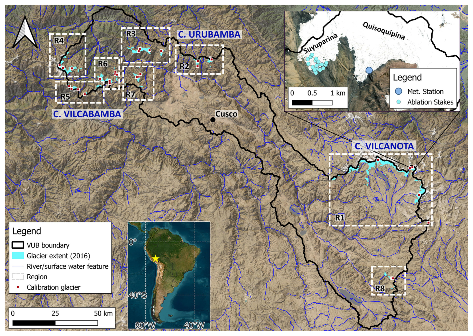
Figure 1 Vilcanota-Urubamba Basin. The inset on the bottom left shows the location of the basin in South America. The inset on the top right shows Quisoquipina and Suyuparina glaciers, with the meteorological station and ablation stake network also marked. The satellite imagery is sourced from Esri World Imagery: Esri, Maxar, Earthstar Geographics, and the GIS user community.

2.3 Climate data

Hourly historical meteorological variables, including near-surface air temperature, wind speed, total precipitation, specific humidity, surface air pressure, and incident shortwave and longwave radiation were taken from the Weather Research and Forecasting (WRF) model, run from 1980 to 2018, with an outer domain with 12 km grid spacing and inner domain covering the VUB with 4 km grid spacing. The precipitation and temperature variables were corrected for bias using station data from within and around the VUB. Equivalent data for the other variables were not available, and as such these were not adjusted for bias. The bias-corrected temperature and precipitation outputs were used as the “historical truth” to statistically downscale 30 global climate models from the Coupled Model Intercomparison Project 5 (CMIP5) to provide a 30-member ensemble of “future” hourly temperature and precipitation driving data from 2019 to 2100 for both Representative Concentration Pathway (RCP) 4.5 and RCP8.5 emission scenarios. The statistical method used was a variation on quantile mapping, following Cannon et al. (2015). This statistical method preserves the trends in the original CMIP5 models, while adjusting the absolute magnitude of temperature and precipitation and the number of wet days. While statistical downscaling methods like quantile mapping have been applied widely to temperature and precipitation variables in the past, they are not routinely used for other variables such as wind and radiation because of the weaker direct link between these variables across spatial scales. For example, a future increase in meridional near-surface wind in the CMIP5 models would not necessarily translate into a future increase in near-surface wind at the WRF model resolution due to the influence of local-scale topography. Similarly, radiation change may depend more on local temperature and humidity variability than large-scale radiation change. An additional challenge of applying statistical downscaling techniques to the other meteorological variables would have been the lack of validation data as the meteorological stations in the VUB only provide temperature and precipitation variables. For these reasons, we decided not to attempt to statistically downscale the CMIP5 projections of the other variables as this could have introduced additional unknown biases in our input data. Instead, equivalent future data for the other meteorological variables were generated by resampling (repeating) the 1980–2018 WRF simulations to produce a continuous 2019–2100 time series. By resampling in this way, we preserve the year-by-year sequencing of the climate variables. This approach was deemed preferable to randomly resampling the data as it preserves any multi-year cycling, e.g. El Niño–Southern Oscillation, which may be present in the driving data. The data were manually checked to ensure that this approach did not introduce any strange jumps in the driving data across the 2018 to 1980 crossover. Full details of the WRF modelling setup, the bias correction and the future statistical projections can be found in Potter et al. (2023).

In addition to the gridded climate data, daily on-ice meteorological measurements between May 2012 and October 2016 were made available after the work by Suarez et al. (2015). These were collected using an automatic weather station, which was situated in the ablation zone of Quisoquipina glacier (5180 m a.s.l.) in the north-east of the VUB (top-right inset of Fig. 1). The measurements include air temperature, relative humidity, incoming and outgoing shortwave and longwave radiation, wind speed, and wind direction.

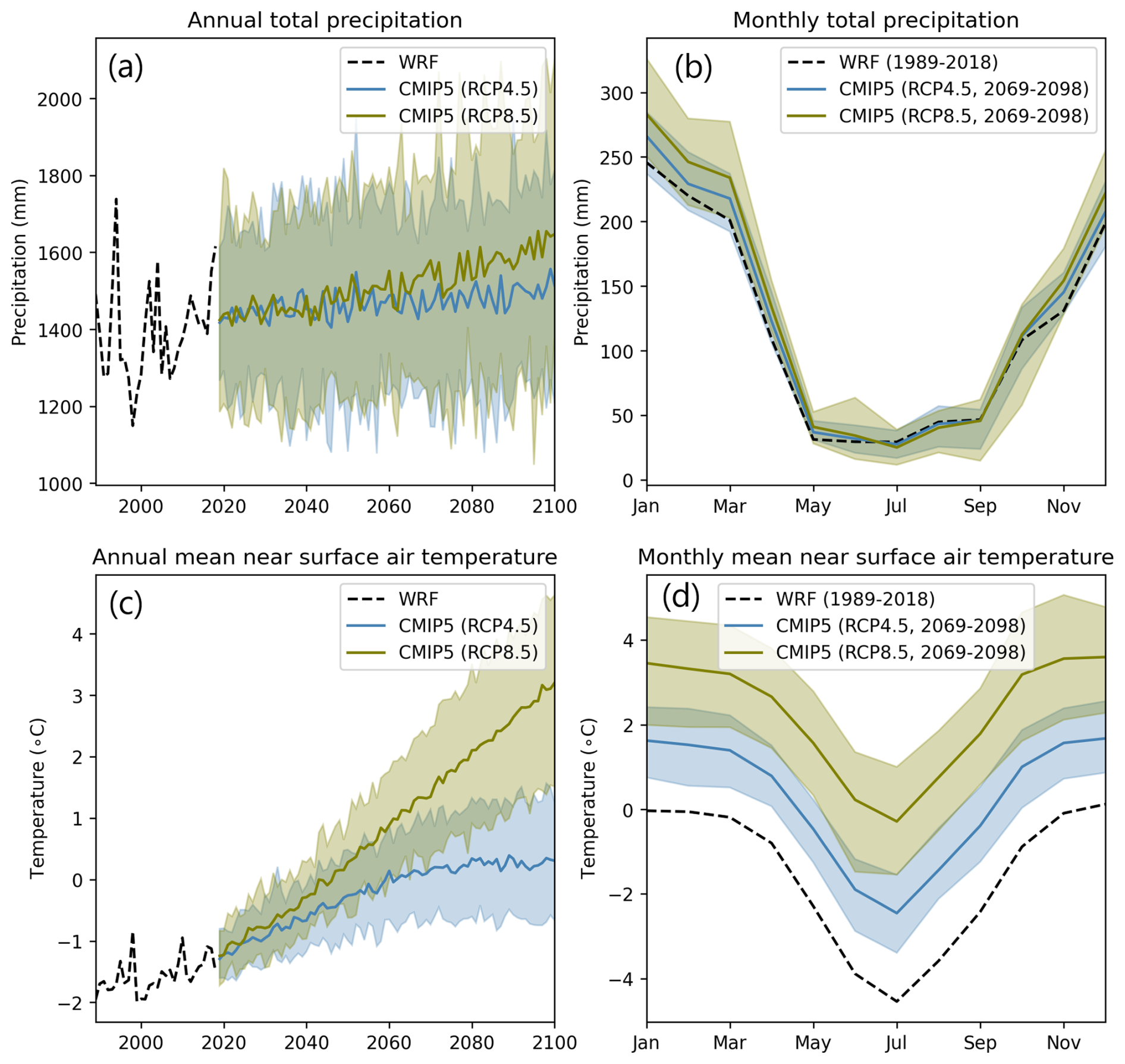
Figure 2 Mean annual on-ice precipitation (a) and temperature (c) and monthly average on-ice precipitation (b) and temperature (d) based on a single WRF historical climate simulation and ensemble of CMIP5 simulations with 90 % confidence bounds. Data taken from Potter et al. (2023).

2.4 JULES–OGGM glacier modelling workflow

JULES–OGGM is a workflow for simulating glacier evolution with climate forcing using the physically based energy balance and ice flow modelling schemes in JULES and OGGM, respectively. It facilitates the exchange of data and feedbacks between these models. This section describes the approach used to integrate them into a single workflow. The reader is referred to Best et al. (2011) and Maussion et al. (2019) for a more detailed explanation of the models.

2.4.1 Climate data pre-processing

JULES requires continuous time series of meteorological forcing variables, including near-surface air temperature, incident longwave and shortwave radiation, air pressure, specific humidity, and precipitation. The approach to deriving these is likely to be specific to each application. In the VUB, given glaciers are small (<8 km²) relative to WRF node areal coverage (16 km²), hourly driving data for each glacier were extracted from the climate model node closest to the centroid of the glacier. Analysis of temperature, surface air pressure, and specific-humidity simulations from WRF, when taken from the model nodes in the vicinity of the glaciers, showed lapse rates with a systematic seasonal cycle (Appendix A). Accordingly, 30 d moving-average hourly lapse rates were calculated for each glacier individually as estimated from the four nodes surrounding the glacier centroid. The median of these was then taken to estimate a regional lapse rate. This averaging step was necessary to remove what were deemed to be unrealistically high or low lapse rates inferred at some glaciers. Analysis of downward shortwave radiation and wind speed indicated no clear lapse rate, and thus these were assumed to be constant with elevation. However, incident shortwave radiation was adjusted to account for the fact that the glaciers have a tilted surface, whereas the flux from WRF is for a flat horizontal surface. The ratio of the direct incident shortwave radiation received on a tilted surface with respect to a horizontal surface can be calculated from the geometric factor, i.e. $R_b=\cos \mathit{\theta }/\cos {\mathit{\theta }}_{\mathrm{z}}$, where θ is the angle of incidence and θ_z is the solar zenith angle. We calculated hourly R_b over the simulation period using glacier slope and aspect derived from the Shuttle Radar Topography Mission (SRTM) digital elevation model and hourly simulations of the position of the sun in the sky that were calculated using the Pysolar Python package (version 0.11) (Stafford, 2023). The WRF incident shortwave radiation flux includes both direct and diffuse shortwave radiation. By default, JULES assumes that half of the incident shortwave radiation is direct, and there was no clear justification to change this. Accordingly, the adjustment was only applied to half of the shortwave radiation flux provided by WRF. Downward longwave radiation is internally adjusted for elevation within JULES as a function of temperature following Shannon et al. (2019). Given the potential for significant bias in precipitation at high elevation due to the lack of observation data, the precipitation lapse rate was reserved as a calibration parameter.

2.4.2 JULES

JULES resolves land surface processes, including the surface energy balance. The model domain is discretized into one or more grid box nodes that can be further discretized into tiles to incorporate sub-grid heterogeneity of the land surface and subsurface, e.g. ice cover and soil properties, respectively. Each grid box node resolves mass and energy fluxes in the vertical direction only. Because of this, computational efficiency can be improved by specifying the model grid as a set of discontinuous grid box nodes where spatially continuous outputs are not required. In the same vein, runtime may be improved by switching off process schemes entirely. Of relevance to glacier modelling is the multi-layer snowpack scheme. The scheme solves the full energy balance at the surface, given atmospheric forcing, following Eq. (1):

$$\begin{array}{}\text{(1)}& \begin{array}{rl}{C}_{\mathrm{s}}{\displaystyle \frac{\mathit{\delta }{T}_{\ast }}{\mathit{\delta }t}}& =\left(\mathrm{1}-\mathit{\alpha }\right){\mathrm{SW}}_{\downarrow }+\mathit{ϵ}{\mathrm{LW}}_{\downarrow }-\mathit{\sigma }\mathit{ϵ}{\left(T_{\ast }\right)}^{\mathrm{4}}-H\\ & -L_{\mathrm{c}}E-G,\end{array}\end{array}$$

where C_s is the heat capacity of the surface (J m⁻² K⁻¹), T_∗ is the surface temperature (K), α is the surface albedo, SW_↓ in the downward solar radiation at the surface (W m⁻²), σ is the Stefan–Boltzmann constant (W m⁻² K⁻⁴), ϵ is the surface emissivity, LW_↓ is the downward longwave radiation at the surface (W m⁻²), H is the turbulent heat flux (W m⁻²), L_c is the latent heat of condensation of water at 0 °C (J kg⁻¹), E is the turbulent moisture flux (kg m⁻² s⁻¹), and G is the heat flux to the material beneath (W m⁻²).

The snowpack scheme simulates vertical heat transfer between snowpack layers, snow compaction, ageing (grain size and darkening), and age- and density-dependent albedo evolution simulated using a prognostic albedo scheme based on the Wiscombe and Warren (1980) spectral snow model. Rainfall on the snowpack percolates through the layers if the pore space is sufficiently large, while any excess water contributes to surface runoff. Liquid water below the melting temperature can refreeze. Shannon et al. (2019) configured a 0.5° JULES model to simulate global glacier volume projections for the 21st century. Each grid box was configured with 46 tiles that had elevations ranging from 0–9000 m in increments of 250 m. For each grid box with glacier coverage, an initial dense ice layer at the base of the snowpack was included with proportional ice coverage across the tiles according to the cumulative observed hypsometry of glaciers within each grid box. Using hourly climate forcing data. Shannon et al. (2019) simulated changes in glacier volume but without any representation of ice flow.

In this study, version 6.0 of JULES was used, with a 10-layer snowpack and ice pack being used following Shannon et al. (2019). The first nine layers include 5 m of snow and firn with depths of 0.05, 0.1, 0.15, 0.2, 0.25, 0.5, 0.75, 1, and 2 m. The bottom layer was used to represent ice with a given thickness of 500 m and initial density of 917 kg m⁻³. The thickness was arbitrarily large to ensure that the entire ice thickness did not melt out at any JULES node during the simulation period. Given the thickness of the bottom layer and the fact that JULES does not account for layer density in its estimation of liquid water holding capacity, this capacity was set to zero to prevent excessive liquid water storage and refreezing. The snow and ice layer density, grain size, temperature, and albedo were dynamically initialized using 20 years (1981–2000) of hourly historical climate data. All model parameters, except those perturbed as part of the model calibration exercise (detailed below), were set to default values. All JULES modelling was performed on the UK NERC-JASMIN high-performance computing facility. A 120-year simulation for a single glacier (10 JULES grid boxes) takes ∼ 25 min to run on a single processor. All 10 JULES grid boxes were used for every glacier to ensure that the glacier hypsometry, regardless of its evolution over the simulation period, was covered by the JULES grid box node elevations.

2.4.3 OGGM

OGGM simulates glacier surface mass balance and ice flow. For any glacier with geometric and climate forcing data, OGGM represents it as one or more connected flowlines that are discretized into nodes and parameterized with approximations of glacier width, area, thickness, and bed shape. Ice flow is simulated by solving the continuity equation along each flowline:

$$\begin{array}{}\text{(2)}& {\displaystyle \frac{\partial S}{\partial t}}=w\dot{m}-\mathrm{\nabla }\cdot uS,\end{array}$$

where S is the area of the cross-section perpendicular to the flow line, w is the width of the cross-section, $\dot{m}$ is the mass balance [kg m⁻² s⁻¹], and u is the average ice flow velocity (m s⁻¹), which includes ice deformation (u_d) and basal sliding (u_s). The ice deformation component is calculated using the shallow-ice approximation:

$$\begin{array}{}\text{(3)}& u_{\mathrm{d}}={\displaystyle \frac{\mathrm{2}A}{n+\mathrm{2}}}h{\mathit{\tau }}^n,\end{array}$$

where A is the ice creep parameter (s⁻¹ Pa⁻³), h is the local ice thickness, τ is the basal shear stress, and n is the exponent in Glen's flow law. OGGM has an in-built temperature index model that runs alongside the ice flow model to simulate glacier evolution given temperature and precipitation forcing data.

OGGM version 1.4 with the default parameterization for ice dynamics (n=3, $A=\mathrm{2.4}\times {\mathrm{10}}^{-\mathrm{24}}$ s⁻¹ Pa⁻³, and u_s=0 m s⁻¹) was used throughout this study. The initial glacier hypsometry and thickness was established using the in-built OGGM functionality based on the glacier outlines from Drenkhan et al. (2018) and the SRTM digital elevation model. Here, ice thickness is estimated at each flowline node by solving the steady-state ice flow at each node. To do this, OGGM version 1.4 uses an “equilibrium mass balance” profile, where the cumulative mass balance across the glacier sums to zero. The thickness at each node is derived from the cumulative upstream surface mass balance. OGGM uses the in-built temperature index model to generate the equilibrium mass balance. For JULES–OGGM, this feature was bypassed, and an equilibrium mass balance for each glacier was instead derived from the calibrated JULES model simulation over the historical period (1981–2018). To satisfy the equilibrium mass balance requirement for each glacier, the mean mass balance at each glacier node was scaled to preserve the mass balance–elevation distribution while summing to zero. All OGGM modelling was performed at the UKRI-BGS high-performance computing facility. A 100-year simulation for a single glacier takes ∼ 90 s to run on a single processor.

2.4.4 Sequential coupling of JULES–OGGM

The basic principle of the JULES–OGGM workflow is to bypass the temperature index model in OGGM and drive the ice dynamics flowline model with surface mass balance simulations from JULES, i.e. substituting $\dot{m}$ in Eq. (2) at each OGGM flowline node. Given the elevation dependence of surface energy balance dynamics, JULES–OGGM must also account for influences of glacier geometry changes on surface mass balance. A workflow has been established that meets both of these requirements through two consecutive modelling steps that does not require dynamic model coupling.

• Step 1: generating mass balance data for each glacier using JULES.

  Each glacier is represented by N ice-covered JULES grid boxes with elevations that are equally spaced between z_min and z_max. For this study, z_min and z_max were set to 4000 and 6500 m a.s.l., respectively, over N=10 grid box nodes that are equally spaced by ∼ 278 m elevation. These elevations do not change during a simulation. The elevation range was instead selected to bound the elevation of all glacier ice over the simulation period, while N was selected to provide adequate representation of changes in mass balance with elevation. Climate data are pre-processed for each grid box using the prescribed lapse rates to represent the climate at that elevation for each glacier. JULES is configured to output annual accumulated snow and ice mass change (specific mass balance) at each grid box elevation of each glacier (hypothetical data for single glacier given in Fig. 3a). The outputs from JULES therefore indicate how surface mass balance changes as a function of elevation on each glacier. No other factors affecting the spatial variability in mass fluxes are accounted for at this stage.

• Step 2: driving OGGM with mass balance outputs from JULES.

  To bypass OGGM's built-in temperature index model, the OGGM source code (version 1.4) was modified to include a new function that reads in the mass balance outputs from JULES. For a given glacier, OGGM takes the annual specific mass balance from the JULES simulation over the N grid boxes (Fig. 3b). For each OGGM node of that glacier, the mass balance at the OGGM node elevation is extracted from the JULES grid box simulations (dashed yellow arrows, Fig. 3b and d) using linear interpolation. This approach allows for incrementation of the glacier mass balance with elevation and also implicitly accounts for the elevation feedback to surface mass balance without requiring two-way coupling between JULES and OGGM. The elevation feedback is demonstrated in Fig. 3c, where the subsequent retreat of the glacier over time results in the lowering of the ice surface (Fig. 3e), and OGGM consequently extracts the mass balance from the JULES simulations at lower elevations. OGGM is configured to output annual changes in glacier volume and area.

One important consideration in the presented JULES–OGGM coupling is how the model deals with the varying physics of surface energy fluxes on ice-free and ice-covered regions as a glacier advances and retreats in OGGM. This could be important, particularly when a glacier is advancing, as OGGM considers ice flowing into ice-free nodes in combination with surface accumulation and ablation processes when calculating the redistribution of ice mass into previously ice-free regions. It was decided to ignore these differences, not only because including an ice-free representation in JULES would effectively double the computational costs but also because all evidence suggests that glaciers in the VUB are and will continue to be in a retreat phase over the planned simulation period, which would render any differences in ice-free and ice-covered physics inconsequential. The implications of this simplification for this study and for other studies will be explored further in the discussion.

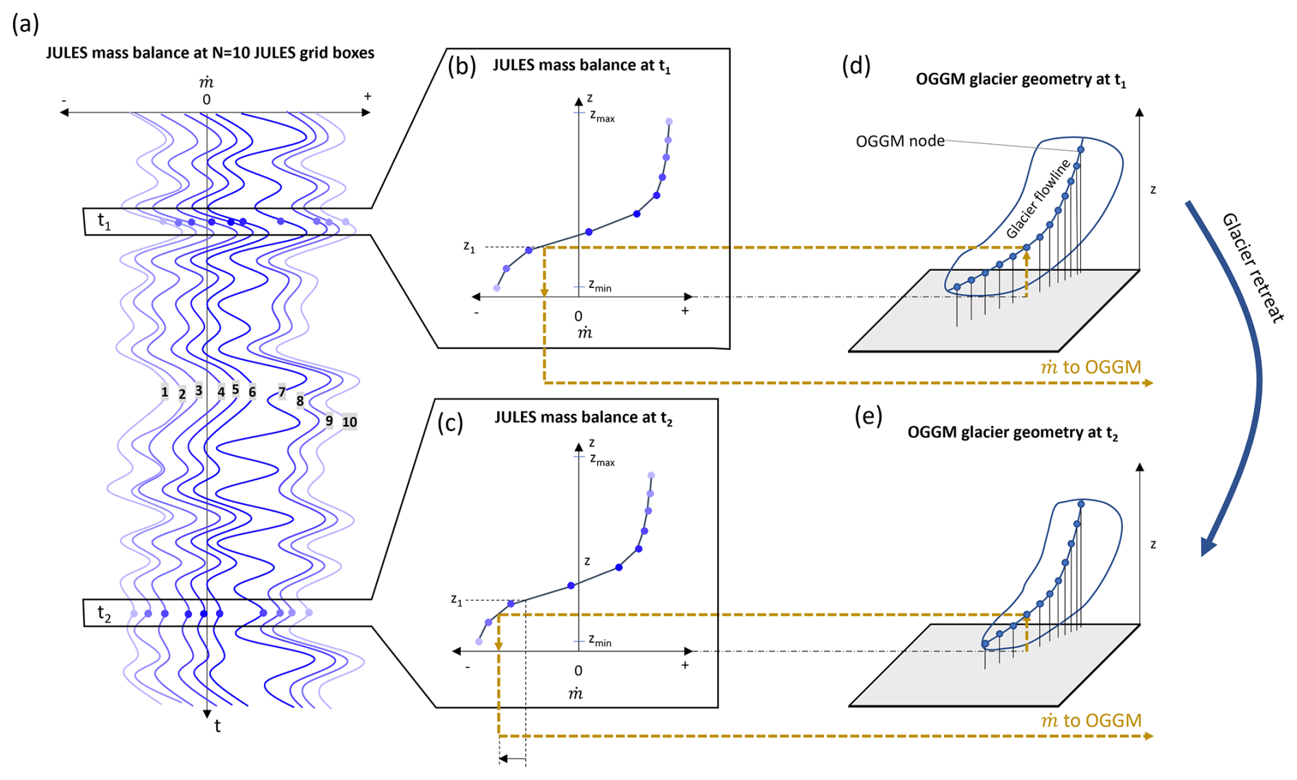
Figure 3 Hypothetical application of JULES–OGGM to single glacier including annual simulated specific mass balance at N=10 JULES grid boxes at different elevations on the glacier (a). The simulated annual mass balance at the 10 grid boxes for time = t₁ (b) and time = t₂ (c). The glacier flowline representation in OGGM at t₁ (d) and t₂ (e). The dashed yellow lines represent the mass balance extraction process from JULES to OGGM.

2.5 Model calibration, evaluation, and sensitivity analysis

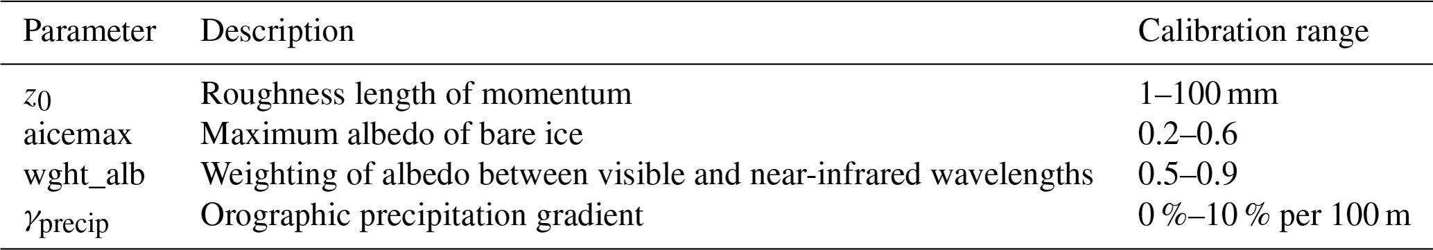
JULES and OGGM both use model parameters that are likely to be spatially variable and cannot easily be constrained from observation data. In this study, only the parameters of the energy balance in JULES were considered for calibration, while the default parameters for the ice flow component of OGGM were used. An iterative calibration strategy was undertaken to tune the JULES parameters to achieve the best fit to the geodetic mass balance data. Firstly, manual perturbations of the JULES model parameters were undertaken to identify those that exhibited sensitivity. We began with all seven parameters identified by Shannon et al. (2019) except for the temperature lapse rate. These include the fresh snow and ice albedo (for visible and near-infrared wavelengths), the precipitation gradient, and a wind speed scale factor. We also included (i) the roughness length of momentum, given its potential importance for sublimation processes; (ii) the temperature threshold below which precipitation falls as snow; (iii) the density above which snow is considered to be firn; and (iv) the weighting of albedo between visible and near-infrared wavelengths. From these experiments, we identified four potentially important parameters for model calibration and suitable calibration ranges (Table 1).

Table 1 Calibration parameters and ranges.

Having established the calibration parameters, model calibration was undertaken using the concept of Monte Carlo whereby random perturbations of these parameters were tested and assessed for their goodness of fit to glacier-wide estimates of specific mass balance over the 2000–2018 period from the geodetic observation data. The aim of the calibration procedure was to select the parameter set for JULES that minimized the sum of the glacier-area-weighted root-mean-square error (RMSE_w). A glacier-area-weighted bias (mean error) was also calculated (BIAS_w). Computational constraints limit the number of glaciers and number of random perturbations that can reasonably be implemented in the framework. Accordingly, a subset of 30 glaciers were identified for the calibration procedure (red squares, Fig. 1) and were selected to include glaciers with a range of elevation, aspect, and slope characteristics and have a good spread across the study basin. Given the uncertainty associated with geodetic measurements of small glaciers, those with the largest overall areas were selected where possible. A total of 1000 random perturbations of the parameters were tested and assessed for their goodness of fit to the geodetic data. The quasi-random Sobol sampling strategy (Bratley and Fox, 1988) was used to sample the parameter space efficiently. All parameters were sampled from a uniform distribution.

The calibration parameters were assessed for sensitivity using the PAWN density-based global sensitivity analysis method (Pianosi and Wagener, 2015) that uses cumulative distribution functions from model outputs conditioned on different parameterizations to estimate sensitivity to different parameters. The PAWN method provides a quantitative, global sensitivity analysis that has been used across environmental modelling applications (Amaranto et al., 2020; Laarabi et al., 2022; Lin et al., 2020). It can be applied to outputs from generic Monte Carlo experiments (Pianosi and Wagener, 2018) and uses the Kolmogorov–Smirnov statistic as the basis for quantifying parameter sensitivity, making it easy to interpret and compute. In this study, we calculated the PAWN sensitivity for each parameter across each calibration using the RMSE_w scores from the Monte Carlo experiment. All analysis was undertaken using the safepython Python library version 0.2.0 (Pianosi and Wagener, 2015). A total of 95 % confidence intervals were estimated for all metrics using the in-built bootstrapping algorithm. Following Pianosi and Wagener (2018), a dummy parameter, which has no impact on the model outputs, was introduced to the analysis to estimate the magnitude of approximation errors.

The calibrated parameters were then incorporated into the basin-wide JULES–OGGM model, which was subsequently evaluated for robustness against the geodetic observations of specific mass balance over all 532 glaciers in the VUB and against the glaciological mass balance observations on Quisoquipina and Suyuparina glaciers.

3 Results

3.1 Model calibration and sensitivity analysis

As a first assessment of the model appropriateness, the optimal simulation from the Monte Carlo experiment was extracted for each glacier individually. Figure 4a shows that for all calibration glaciers it is possible to achieve a close fit to the observed specific mass balance when the calibration parameters are tuned to each glacier separately. JULES–OGGM is able to capture the observed specific mass balance within 0.008 m w.e. of the observations for all glaciers. When the single best parameterization is chosen based on the RMSE_w across all glaciers, the errors are larger (Fig. 4b), ranging between −0.99 and 1.22 m w.e. with an RMSE_w of 0.56 m w.e. It would not be feasible to tune the parameters to each glacier individually. However, a single parameterization appears to degrade the performance of the model significantly. Accordingly, it was decided to investigate if an improved goodness of fit could be obtained by adopting a regional-parameterization approach. Here, we split the calibration glaciers into eight different regions (dashed white boxes in Fig. 1), which in part reflected known differences in glacier hypsometry and driving climate characteristics and ensured that at least two glaciers are obtained within each region. This resulted in eight parameterizations, which resulted in a modest improvement of the RMSE_w to 0.46 m w.e. (Fig. 4c). While the errors remain significant, the errors were reduced for 21 of the 30 calibration glaciers, and the spatial disaggregation makes upscaling the parameterization to all glaciers in the catchment easier. As a result, this regional approach was adopted for the remainder of the study. Note that because of this regional lapse rates were also applied (Appendix A).

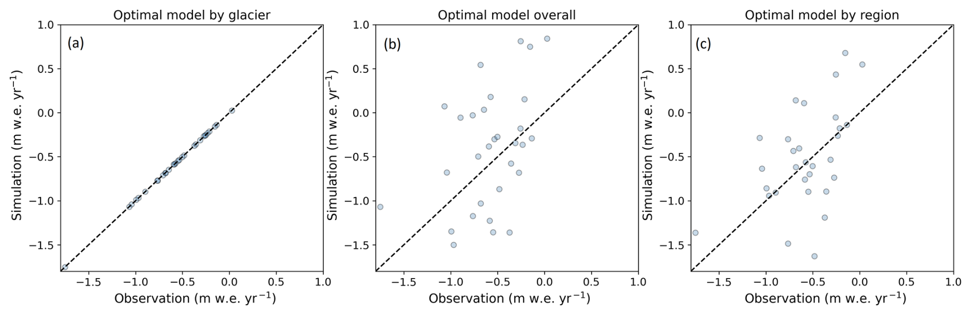
Figure 4 Simulated and observed mean annual specific mass balance over 2000–2018 for the 30 calibration glaciers using different calibrated parameterizations, including those obtained for each individual glacier (a); when using the single best overall parameterization based on the RMSE_w score (b); and when using the models optimized for the eight delineated regions (c).

The RMSE_w and BIAS_w scores range between 0.01–0.73 and −0.06–0.29 m yr⁻¹ w.e., respectively, across the regions (Table 2). The calibrated parameters typically span a large portion of the calibration range. The only exceptions to this is z₀, which does not exceed 7 mm for any of the regions.

Table 2 Calibrated parameter sets from the calibration parameters in Table 1 for each region and RMSE_w and BIAS_w scores.

The PAWN sensitivity analysis reveals that the modelled mass balance is most sensitive to the wght_alb parameter for all of the regions (Fig. 5). Furthermore, for all regions except for R6, the wght_alb parameter is the only parameter with a sensitivity index significantly greater than the magnitude of approximation errors, as shown by the dummy parameter. For R6, the simulated mass balance is also sensitive to the precipitation gradient, i.e. γ_precip. The simulated mass balance shows negligible sensitivity to the aicemax and z₀ parameters for all regions.

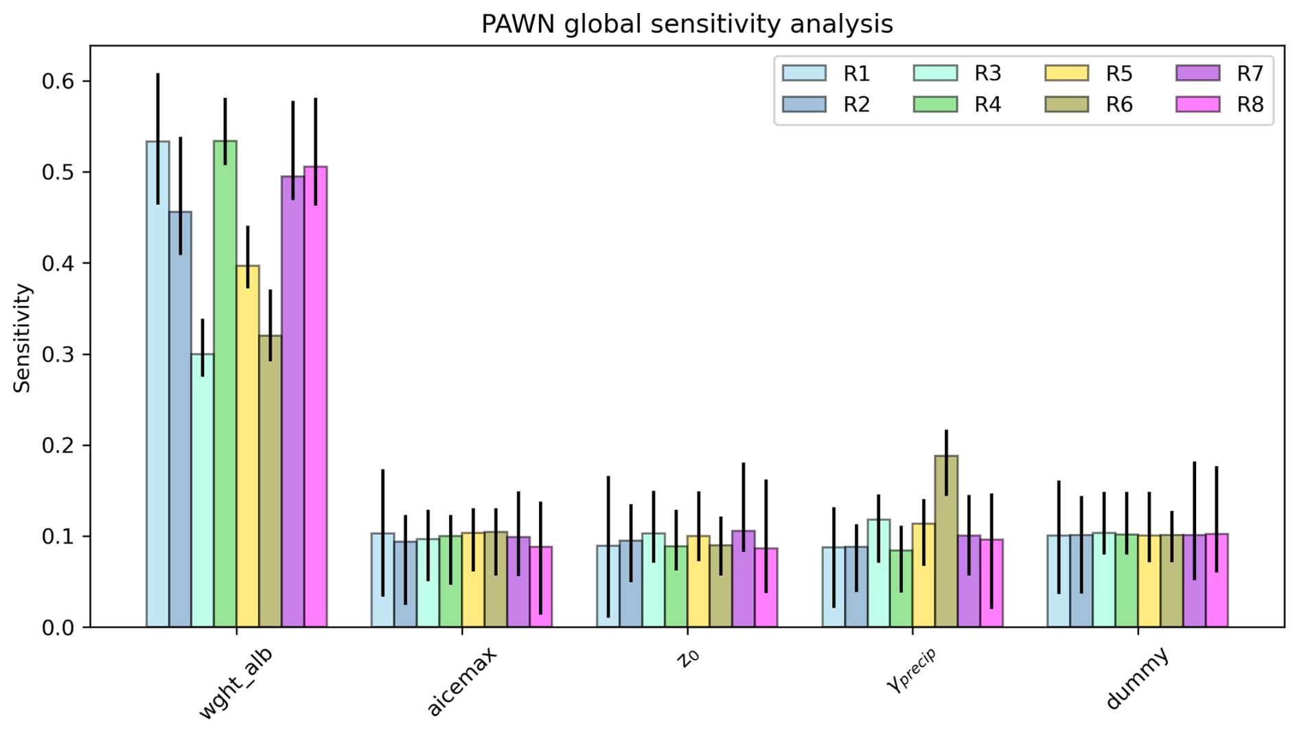
Figure 5 Region-specific PAWN sensitivity metrics and 95 % confidence intervals (black lines) for all calibration parameters and the dummy parameter.

3.2 Model evaluation

3.2.1 Basin-wide mass balance

When applied to all 532 glaciers, the simulated specific mass balance varies considerably, ranging from −4 to +4 m yr⁻¹ w.e., which is in line with the observed range (Fig. 6a). The area-weighted specific mass balance across all glaciers is −1.06 m yr⁻¹ w.e., approximately double that derived from the geodetic observations (−0.52 m yr⁻¹ w.e.), indicating that the model is losing mass too quickly over this period. In addition, the model does not capture within-basin variability in specific mass balance, with absolute errors as high as 3 m yr⁻¹ w.e. The sources of these errors are not clear. When aggregated to 0.05° tiles, there is considerable variability in the magnitude and direction of error across the basin and within the regions (Fig. 6b). A comparison of the mass balance errors to glacier area, aspect, slope, and elevation attributes showed no clear pattern of coherence to glacier characteristics (Fig. B1).

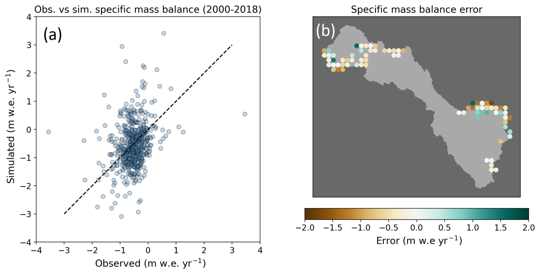
Figure 6 Observed vs. simulated annual-mean specific mass balance (2000–2018) for all glaciers in the VUB (a) and area-weighted annual mean specific mass balance errors aggregated to 0.05° tiles (b).

3.2.2 Glacier volume simulations

A comparison of the estimated glacier volumes from Millan et al. (2022) for the year 2018 against the JULES–OGGM simulation shows that there is generally good agreement, especially for the largest glaciers in the catchment (Fig. 7). JULES–OGGM does, however, show a tendency to underestimate the volume of the smallest glaciers (<10⁻² km³). The total JULES–OGGM ice volume for glaciers where Millan data are available is 7.19 km³, whereas Millan et al. (2022) estimate it as 8.16 km³.

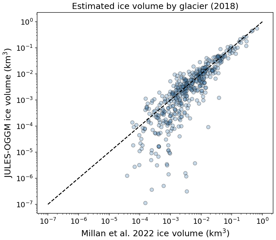
Figure 7 Estimated glacier volumes from Millan et al. (2022) vs. the JULES–OGGM ice volume simulation for 2018 for all glaciers where data are available in the VUB.

3.2.3 Quisoquipina and Suyuparina glaciers

To aid the evaluation of the robustness of the calibrated model parameters, a point-scale JULES model (no ice dynamics) was set up to evaluate against the ablation stake data on Suyuparina glacier. The model was parameterized with the corresponding R1 region parameterization. All WRF-driving climate variables were corrected for bias in the long-term mean using the daily Quisoquipina meteorological station data. Suyuparina and Quisoquipina glaciers are two of the 30 calibration glaciers. Bias correction of the hourly WRF data, rather than the raw daily meteorological station observations, were chosen due to the requirement of hourly data to drive JULES and to ensure consistency with the calibration-driving data. The model was run over an evaluation period of June 2012 to January 2016 as meteorological and ablation data are available for that period.

Using this model, the energy balance simulations (Fig. 8a) show that solar radiation (SW_net) is the dominant energy input for the majority of the simulation period, followed by sensible heat warming from the air (H). Latent heat fluxes (L_cE) are typically negative and smaller in magnitude. The net diffuse radiation flux (LW_net) has a marked seasonality: positive during the wet season (austral summer) when cloud cover is highest and negative during the cooler, clear-sky days during the austral winter. Interestingly, SW_net shows only weak seasonality, with a peak during the wet season. This appears to be related to the behaviour of albedo at the glacier surface (blue line, Fig. 8c), which rarely falls below 0.8 and appears to be highest in the dry season. This is in contrast to the observed albedo (black line, Fig. 8c), which typically peaks during the wet season when there is plentiful fresh snow and falls as low as 0.2 by the end of the dry season when fresh snow cover is minimal and the ice surface has darkened. Indeed, the simulated snow and ice layer density of the top 2 m (Fig. 8e) shows that even during the dry season the top 5–10 cm typically resides at <500 kg m⁻³, representative of old snow. In reality, at the Quisoquipina meteorological station, bare ice is exposed seasonally. The inability to capture ice exposure and darkening through the dry season is consistent with the simulated cumulative ablation (yellow line, Fig. 8g) underestimating observed ablation (black line, Fig. 8g) in 2014. This period is highlighted between the dashed lines in Fig. 8g.

As an additional experiment, the observed daily proportion of outgoing to incident solar and diffuse radiation at Quisoquipina met station were used to convert the hourly WRF radiation inputs to net radiation, which effectively bypasses the prognostic albedo model in JULES. When driving the model in this way it can be seen that the simulated SW_net and surface albedo are much more seasonally variable (Fig. 8b and d, respectively) and that the simulated albedo dynamics are more coherent with the observations. The model also better replicates the seasonal loss of the snowpack (Fig. 8f), where the top 5–10 cm routinely exceeds a density of 700 kg m⁻³. In addition, within the period bounded by the dashed lines in Fig. 8h, the simulated and observed ablation rates (gradients of yellow and black lines, respectively, in Fig. 8h) are more closely matched. Note, however, that the negative bias over the preceding wet season persists.

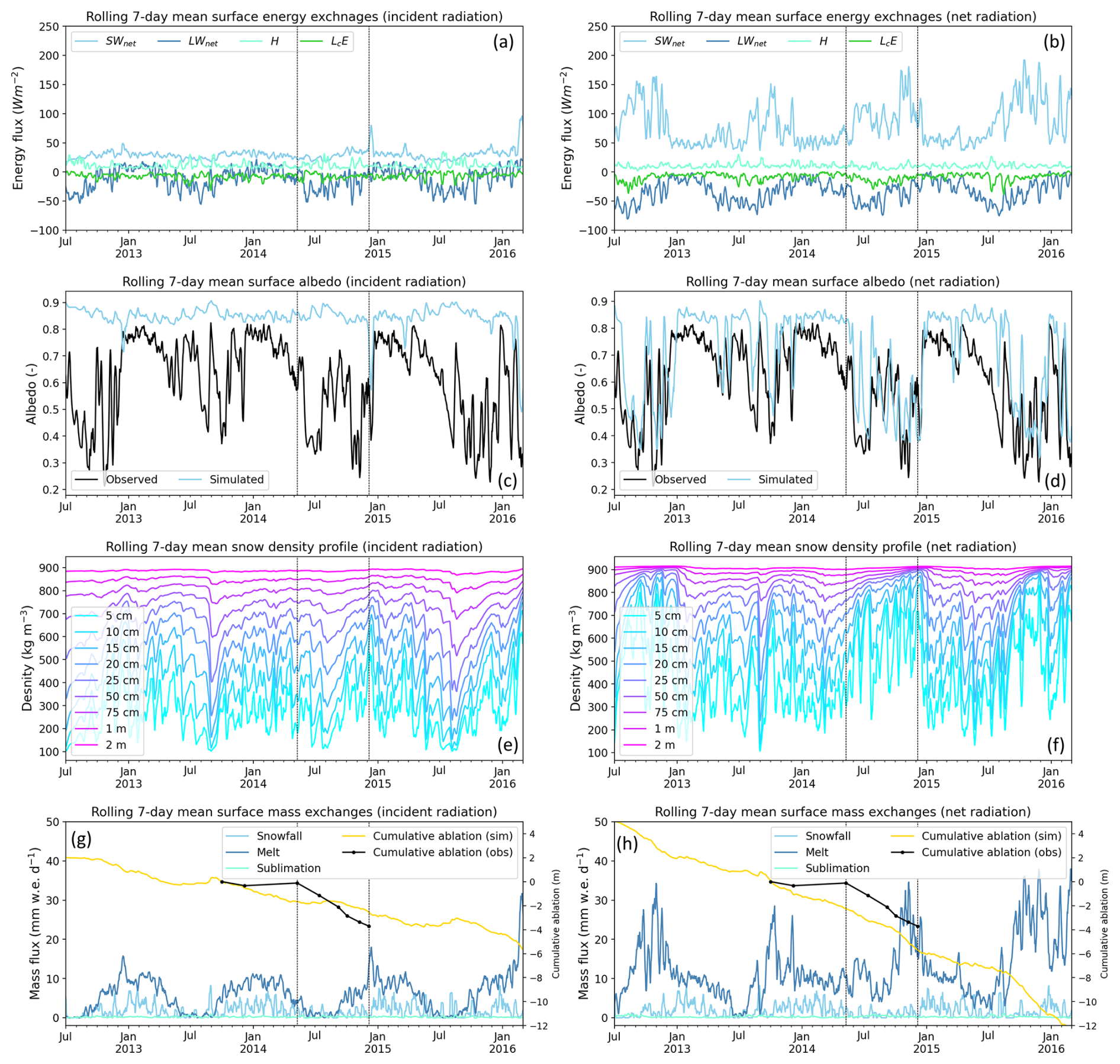
Figure 8 JULES energy balance simulations on Quisoquipina glacier from July 2012 to January 2016 (when local meteorological and mass balance data are available) for the model driven with incident radiation observations (a, c, e, g) and the model driven with net radiation observations (b, d, f, h). All variables are shown as 7 d moving averages for ease of interpretation. Note that sublimation, as output by JULES, is the net effect of sublimation minus the deposition processes.

3.3 Glacier projections for the 21st century

3.3.1 Area and mass evolution

The projections indicate that total glacier area and mass in the VUB have decreased year on year from the year 2000 and will continue to do so to the end of the 21st century under the RCP4.5 and RCP8.5 scenarios (Fig. 9). Relative to 2000, the glacier area is predicted to halve by 2047 (2043) under RCP4.5 (RCP8.5). The glacier mass is predicted to halve by 2027 for both RCPs. This close agreement is likely reflective of the relatively similar temperature and precipitation signal across both RCPs for the early 21st century. By the end of the century, the differences in predictions across the RCPs are more pronounced, with the total glacier area predicted to decrease to 28 % (11 %) of that in 2000, while the total glacier mass predicted to decrease to 17 % (6 %) of that in 2000 for RCP4.5 (RCP8.5).

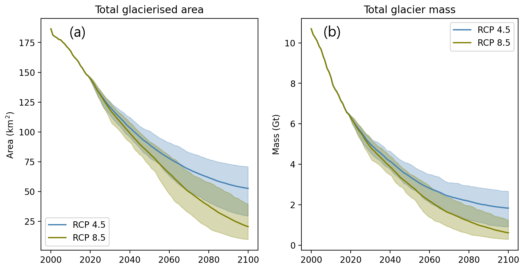
Figure 9 Simulated annual total glacierized area (a) and mass (b) for the VUB between 2000 and 2100 based on RCP4.5 and RCP8.5 scenarios. Each RCP is represented by the ensemble mean (solid line) and 90 % confidence interval (shaded area).

3.3.2 Variability in glacier response to climate change

K-means clustering was used to cluster the glaciers based on their ensemble mean simulated annual glacier mass time series over the future period of 2020 to 2100 under RCP8.5. Four clusters were found to have distinct mass evolution dynamics (Fig. 10a and b). Clusters 1 to 3 all show sustained mass loss over the simulation period, while cluster 4 shows initial mass gain up to the middle of the century that is followed by mass loss for the remainder of the century. The timing of this inflection in cluster 4 is approximately 5 years earlier in RCP8.5. The mass loss rate is greater in RCP8.5 than RCP4.5 for all clusters.

The proportional rate of retreat is progressively smaller from clusters 1 to 4. This corresponds to a progressively higher median elevation (Fig. 10f). At the two extremes, clusters 1 and 4 are typically small in surface area and at low and high elevations, respectively (Fig. 10e and f). Cluster 3 accounts for the largest proportion (>80 %) of glacier mass for the majority of the simulation period (Fig. 10c). This type of glacier is the dominant in the Cordillera Vilcanota in the east of the catchment. The lower-elevation glaciers (clusters 1 and 2) are more prevalent to the west of the catchment.

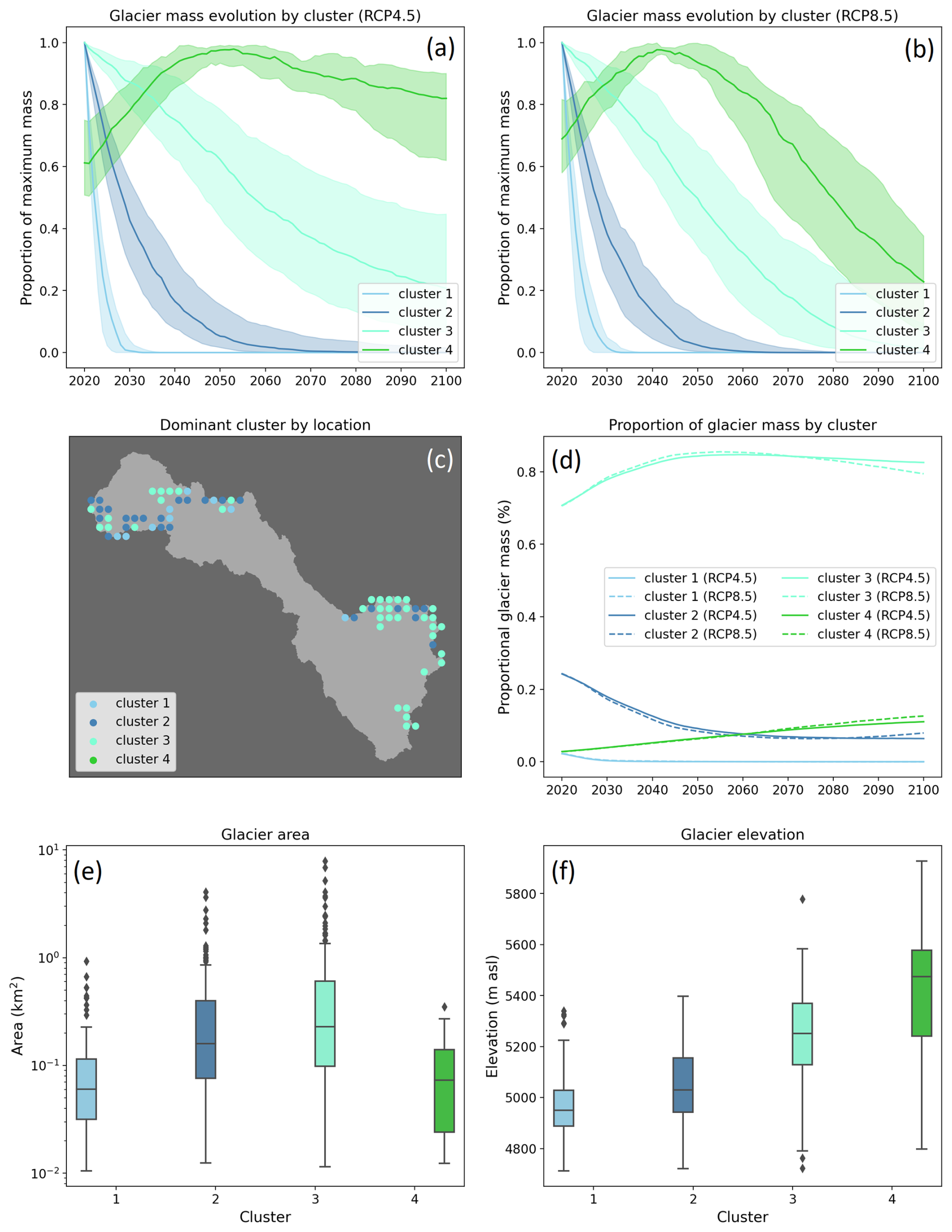
Figure 10 Annual glacier mass evolution of four identified clusters expressed as the proportion of the maximum simulated mass between 2020 and 2100 for RCP4.5 (a) and RCP8.5 (b) taken from the ensemble mean. Each cluster is represented by the median (solid line) and interquartile range (shaded area). The dominant cluster by 0.05° cell (c), the evolution of glacier mass distribution between clusters (d), the spread of glacier area based on initial mapped areas for the year 1998 (e), and the initial elevations based on SRTM elevation data for the year 2000 (f) within clusters expressed as box plots.

3.3.3 Mass and energy balance dynamics

Annual changes in ice elevation, specific mass balance, and energy balance have been calculated for each cluster and RCP combination (RCP8.5 in Fig. 11 and RCP4.5 in Fig. E1). These variables have been calculated as an average across only the active ice area to avoid zero fluxes due to the complete loss of glacier ice. This raises an additional challenge when interpreting the results over an ensemble of climate inputs given that the distribution of glaciers will not be the same across all ensemble members over time. Simply averaging across the ensemble therefore has the potential to obscure co-dependencies between different mass and energy fluxes. Rather than taking the mean over the full ensemble of simulations, we have used a single global climate model simulation (BNU-ESM) from the CMIP5 ensemble that was found to most closely follow the ensemble mean mass evolution of the clusters under both RCPs (Fig. D1).

Mass balance (middle row of Figs. 11 and E1) is consistently negative for all clusters, with the exception of cluster 4, where we see a transition from positive to negative mass balance in the mid to late 21st century. The remaining clusters show a positive trend in mass balance under RCP4.5 but a more mixed response under RCP8.5. These decadal trends are primarily controlled by changes in snowmelt and ice melt. The melt flux is typically more variable over the 21st century than the snowfall input and much higher in magnitude than the net mass flux due to sublimation and deposition, which is only very weakly positive for all of the clusters under both RCPs. Snowmelt and ice melt show some coherence with changes in near-surface air temperature, which is itself a function of climate warming and the retreat of glaciers up to cooler and higher elevations, a trend that is consistent across the catchment (top row in Figs. 11 and E1). The apparent stability in the snowfall input appears to be related to a compensatory effect, where the warming and transition of snowfall to rainfall is counter-balanced by (i) the retreat of glaciers to higher elevations where precipitation rates are higher and a smaller fraction of that precipitation falls as rain and (ii) the increase in total precipitation over time projected by the CMIP5 models. This, however, is only true for the larger glaciers of clusters 2 and 3 that span a large elevation range. For the smaller high-elevation glaciers (cluster 4), the reduction in mass input from snowfall due to rising temperatures is comparable to the magnitude of change in melt and serves to accelerate the retreat of the glaciers.

While there is generally good coherence between the snowmelt and ice melt flux and changes in near-surface air temperature, this co-variability does not always hold. For example, near-surface air temperature over the glaciers in clusters 2 and 3 shows a steady increase from 2040 onwards on average under RCP 8.5 (Fig. 11). The average melt flux increases steadily at first but then more rapidly from 2080 onwards, which is not reflected in the temperature data. Analysis of the surface energy balance components (bottom row in Figs. 11 and E1) reveals that the melt flux is more coherent with changes in net shortwave radiation, which is the dominant source of energy at the snow and ice surface for all clusters under both RCPs and is itself inversely proportional to the surface albedo. While higher temperatures facilitate more melt and inhibit snowfall, thereby lowering the albedo, it is changes in net shortwave radiation that primarily control decadal variability in melt rates and surface mass balance. Turbulent heat fluxes are smaller than radiative energy fluxes for all clusters and RCPs. Sensible heat fluxes typically increase with time, presumably due to the rising air temperature, while latent heat fluxes decrease.

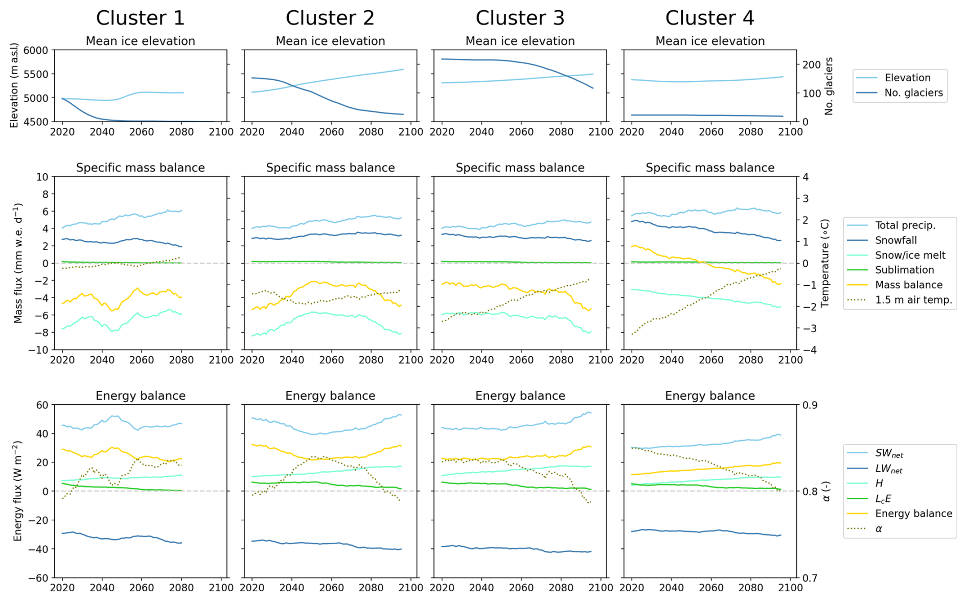
Figure 11 Simulated mean glacier-wide state variables from JULES–OGGM between 2020 and 2100 for each cluster (columns) and based on the BNU-ESM simulation under RCP8.5. The variables include ice elevation (top row), specific mass balance (middle row), and energy balance (bottom row). All variables are calculated over a 10-year moving-average window and are taken as the mean across all glaciers within a cluster as weighted by the glacier area.

4 Discussion

4.1 Model performance and limitations

The model calibration experiments suggest that the energy balance parameters in JULES–OGGM can be tuned to capture the decadal (2000–2018) glacier-wide mass balance of a range of glaciers in a tropical setting with a small error (<±0.01 m yr⁻¹ w.e.). This is encouraging for the future use of physically based models for modelling tropical glacier evolution. However, attempts to extrapolate these parameters across all 532 glaciers in the VUB resulted in inconsistencies in model performance. This extrapolation step was required given that the Monte Carlo calibration approach was too computationally demanding to afford tuning the model parameters to all glaciers individually like, for example, Aguayo et al. (2024), who tuned the parameters of a simpler temperature index model in OGGM for all of the glaciers in the Patagonian Andes. A more efficient calibration routine or the availability of sufficient computational resources would be required to calibrate the JULES parameters in this way. However, this approach would need careful consideration of how this model could reasonably be “validated” outside of its calibration data. One could also argue that the inherent uncertainties in geodetic mass balance data, particularly for the smallest glaciers (Dussaillant et al., 2019), could lead to significant model biases. In the same vein, it is fair to assume that at least some of the apparent model inconsistencies are themselves manifestations of the uncertainty in the geodetic validation data. While this may be true, the assessment of the model fit to the 30 calibration glaciers, which were chosen for their relatively large size, showed similar levels of inconsistency, which suggests the overall impact on interpretations of model deficiencies is minimal. In fact, the use of the geodetic data for calibration, we would argue, is more justifiable than using sparse glaciological data for this tropical setting. Indeed, when Shannon et al. (2019) calibrated JULES using a similar approach to that used here but with elevation-band specific mass balance observations from the World Glacier Monitoring Service (WGMS, 2023), their model showed an unrealistically negative bias for low-latitude regions.

Other improvements to the calibration strategy that could provide gains in model performance include a more suitable grouping of glaciers that better captures the differences in glacier properties (and model parameters) instead of the location-based regionalization implemented in this study. What the basis would be for this grouping, however, is not clear from this study, given that there was no clear coherence between simulated mass balance errors and glacier characteristics. One should also consider that the ice flow parameters in OGGM were not considered in the calibration procedure. This has obvious implications for the simulated ice dynamical response to climate forcing and for the initial ice thickness inversion step, both of which have the potential to introduce errors into the forward projections. The recent work of Aguayo et al. (2024) has shown how the OGGM creep parameter can be included in the calibration of OGGM. They propose a method whereby the this parameter is selected so that the ice thickness inversion step, used to identify the initial ice volume, matches that of an independent set of glacier volume estimates similar to those of Millan et al. (2022). Within their calibration routine, the model is further validated against RGI glacier outlines for the year 2000 by implementing a “dynamic spinup” of the model from 1980. Only when the model can capture the RGI glacier area, the glacier volume estimates, and geodetic mass balance data is the calibration deemed a success. Implementing this type of calibration approach with JULES–OGGM is feasible, although it comes with its own computational constraints that would not make this straightforward. Even so, it could be that additional gains in model performance are found by considering the ice dynamical parameters in the model calibration.

While modifications to the calibration strategy may be beneficial to model performance, the expected benefits can only be postulated here. This study suggests that meaningful improvements in model performance could be attained through targeting improvements to the prognostic snow albedo routine in JULES. Specifically, it appears that the model cannot accurately replicate the feedbacks between the driving meteorology, surface energy balance, ablation processes, and snow darkening. Because of this, the calibration problem was dominated by the sensitivity to the parameter that controls the weighting of albedo between visible and near-infrared wavelengths (wght_alb) in JULES: a parameter that is important in controlling the rate at which snow albedo drops as the snow ages and grain size increases. While this parameter can be tuned to capture long-term average estimates of glacier-wide mass balance, comparisons of simulated and observed surface albedo at the Quisoquipina meteorological station revealed an apparent case of “correct answer for the wrong reason”: a case that is likely to manifest itself in inconsistent performance outside of the spatiotemporal bounds of the calibration dataset. Only by forcing this aspect of the model with observed net radiation variables were we able to more-accurately capture day-to-day and seasonal variability in surface albedo and the observed ablation rates during the main ablation season. The prognostic snow albedo routine in JULES is based on the Wiscombe and Warren (1980) spectral snow model, which simulates changes to snow albedo in both the visible and infrared wavelengths as a function of effective snow grain size. The models of snow grain size development and spectral albedo are, in essence, empirical and validated against a small number of observation studies in the Antarctic and Canadian Archipelago, which raises the question of their validity in other settings. They also highlight two limitations of the model in the inability to account for (i) snow impurities and (ii) scattering properties of non-spherical snow grain shapes. Ice cores drilled from the Quelccaya ice cap on the eastern edge of the VUB show seasonal deposition of mineral dust during the dry season when westerly winds facilitate entrainment and transport from the dry Altiplano (Thompson et al., 2013). Reis et al. (2022) found that the average dry season dust concentration between the years 2002 and 2018 was 6.8 ± 1.8 ppm but could be as high as 23.1 ppm. A limited number of observation studies suggest that black carbon concentrations of less than 1 ppm can reduce snow albedo by several percent but that the effect of mineral dust is approximately 2 orders of magnitude smaller (Willeit and Ganopolski, 2018). However, recent numerical modelling studies suggest that the impact of mineral dust on snow albedo could be much more significant and is strongly influenced by snow grain size and non-sphericity. He et al. (2019) explicitly simulated the deposition and redistribution of dust through the snowpack and the scattering properties of non-spherical snow grain shapes in the stochastic aerosol–snow albedo model (Liou et al., 2014) and showed that snow albedo can be reduced in the visible wavelength spectrum by almost 20 % when the dust concentration is 100 ppm and the snow grain radius exceeds 1000 µm, although the magnitude of reduction is dampened for non-spherical snow grains. Hao et al. (2023) demonstrated that including these processes in the E3SM land surface model allowed them to more closely match observed albedo dynamics on the Tibetan Plateau. However, they highlight that the combined effects of non-sphericity and snow impurities on albedo are complex, non-linear, and may be negative or positive depending on the approach used to parameterize them. The composition of other impurities, e.g. biological communities that could also serve to reduce snow and ice albedo (Hotaling et al., 2021), have to our knowledge not been observed or quantified in the study region. Thus, while gains could be made through implementing improvements to the prognostic snow albedo routine in JULES, such improvements would need to be underpinned by appropriate observation data to appropriately parameterize them. Meeting this challenge will undoubtedly require improvements to our process models but likely also requires us to better constrain mountain snowfall timing and frequency, which have a significant influence on albedo dynamics (Johnson and Rupper, 2020).

4.2 The “ice-free” limitation

In the methodology, we noted that the JULES–OGGM sequential coupling does not explicitly account for differences between surface energy balance fluxes on ice-free and ice-covered surfaces, which could be important when OGGM determines if a glacier will advance into an ice-free node on a given time step. For ice-free nodes, OGGM takes the sum of the surface mass balance and ice flowing into that node from upstream. If this sum is positive, the glacier “grows” into this node. With the presented JULES–OGGM setup, the surface mass balance for the ice-free node is calculated as though it were covered by ice. This means that there could be some situations where JULES–OGGM simulates the advance of a glacier at a given time step when an identical model that accounts for the ice-free energy balance does not (and vice versa). As a thought experiment, we could hypothesize a JULES–OGGM model that has an equivalent set of ice-free JULES grid box nodes for each glacier spanning the full elevation range of the glacier. We could then force OGGM with surface mass balance simulations that are tailored to the ice coverage conditions at a given point in time. The overall impact that using such a model would have on the simulation is difficult to postulate given that it will depend a lot on how the exposed ground is parameterized in JULES, but we would hypothesize that sensitivity to this model limitation would be most pronounced for (i) advancing glaciers where the surface mass balance will impact the ice thickness at the margin during transition from an ice-free to ice-covered state and (ii) glaciers where simulated mass balance at the tongue is close to zero, meaning that small changes in the simulated mass balance on ice-free nodes could decide whether or not a glacier grows at a particular time step. For glaciers undergoing sustained retreat where the surface mass balance at the glacier margin is consistently negative, the choice of using JULES–OGGM with or without our hypothetical improvement would have no discernible effect on the simulation. For this reason and the fact that the mass balance of the glaciers in the VUB over the simulation period is negative (particularly at the glacier tongue), we would argue that discrepancies introduced by the ice-free limitation are likely to be small in this study.

4.3 The 21st-century simulations

Considerable variability in glacier response to climate exists across the VUB. We identified four broad mass evolution clusters, ranging from glaciers that lose most (if not all) of their mass before 2040 to those that showed an initial mass gain before subsequently retreating through the latter half of the 21st century. While the exact trajectory of the simulations needs to be considered within the limitations of the model, the results suggest that the dominant control on this variability is the glacier geometry. Specifically, the smallest glaciers at low- and high-elevation ranges represented the most and least rapidly retreating glaciers, respectively. Fyffe et al. (2021) also found that elevation plays an important role in controlling the non-linear response of tropical glaciers to changes in air temperature. At higher elevations, they suggest that decadal changes in mass balance are more strongly controlled by the transition of sublimation fluxes to melt. While this may be true at very localized high-elevation ice, we did not find any evidence of significant sublimation fluxes at the river basin scale. In fact, for all identified clusters, sublimation made a negligible contribution to annual glacier mass changes throughout the simulation period. This does raise the question of the gains achieved through applying energy balance models for basin-scale analyses like these and whether we should sacrifice the level of fit that can be achieved with a simpler temperature-based ablation model just for the sake of providing a more physically coherent model of the system. We suggest that this depends on the purpose of the application and the region of interest. The apparent insignificance of sublimation in the VUB should not be expected everywhere. Furthermore, our simulations still showed deviations between long-term temperature and mass balance trajectories. Specifically, the shortwave radiation was shown to be the dominant energy source across the glaciers and is controlled by the surface albedo, which was not necessarily coherent with temperature. Given the importance of shortwave radiation, a key limitation of the projections is that this variable was effectively assumed to be static for the future simulation period, and therefore the projections do not capture the impact of changes in the radiation balance in the future. To explore this limitation in more detail, we extracted the incident longwave and shortwave radiation data from each CMIP5 ensemble member at the point closest to the middle of the domain (at −13.69° N, −72.02° E). These data showed that the annual average incident longwave radiation is projected to increase by an average of 6.63 % from the 1980–2018 average to the 2061–2099 average under RCP8.5, with all models showing a statistically significant increase. These data also showed an increase in average incident shortwave radiation by 3.20 % over the same time period, with 22 models showing a statistically significant increase, 4 showing a statistically significant decrease, and 4 showing no significant change. While these changes would only result in a relatively small change in the radiation balance, they are not accounted for in our projections.

To provide some context for the simulated ice area and mass simulations, we obtained simulations for the VUB from the GlacierMIP experiments (Marzeion et al., 2020) for the GloGEM (Huss and Hock, 2015) and MAR2012 (Marzeion et al., 2012) models. These models are much simpler than JULES–OGGM, using temperature-based energy balance models and empirical ice evolution routines to account for mass redistribution. When driven with the same CMIP5 GCMs, the overall trajectory of total glacier area and mass is broadly similar across the three models (Fig. C1), showing a consistent decrease over time. However, JULES–OGGM is shown to be more conservative (slower retreat), particularly with respect to the change in glacier area. Under RCP4.5, JULES–OGGM estimates that 17 % of the ice mass will remain by 2100, while GloGEM and MAR2012 estimate this to be 2 %. For RCP8.5, JULES–OGGM estimates that 6 % of the ice mass will remain, while GloGEM and MAR2012 predict that less than 1 % will remain. These differences likely stem from a range of sources in addition to differences in the glacier models themselves. Arguably of major importance is the fact that JULES–OGGM was shown to overestimate surface albedo at one observation point in the basin, at least at the one observation point in the basin. If this behaviour is indicative of basin-wide simulations, the apparent conservativeness of the simulated retreat likely stems from this model deficiency. Additionally, as has been discussed, we did not use the raw CMIP 5 climate projections used to force the GloGEM and MAR2012 projections. Instead, we used a combination of statistically downscaled and resampled driving climate data that will have inherently different biases and trends over the 21st-century simulation period. Aguayo et al. (2024) compared the impact of perturbing various aspects of the model setup for OGGM on glacier runoff simulations for the Patagonian Andes and showed that the uncertainty in simulated glacier runoff mainly stemmed from the choice of historical climate data used to calibrate the model for 78 % ± 21 % of the catchment area. In contrast, “future” sources of uncertainty (choice of climate model, emission scenario, and method of bias correction) were only the main sources of uncertainty for 18 % ± 21 % of the catchment area. Similarly, Li et al. (2022) showed that the projected mass loss difference between two identical glacier dynamics models of central Asia with different initial glacier inventories was higher than that of adjacent emission scenario forcing data.

Aguayo et al. (2024) also showed the significance of other aspects of the model setup, such as the initial ice thickness and glacier outline maps. Indeed, our study used the more refined glacier outline maps of Drenkhan et al. (2018) than those in the GlacierMIP, and there are clearly differences in our initial glacier areas that we estimate to be significantly smaller (186.5 km²) compared to those from the GlacierMIP models that are based on the less accurate RGI 6.0 glacier outlines (250.1–264.3 km²). For the initial ice volume, it is important to note that our simulated ice mass for the year 2000 lies somewhere between that of GloGEM and MAR2012 (Fig. C1c and d), which suggests that this is not a principal driver of the differences in our simulations to these models. When we compared our ice volume simulations for 2018 against the estimates of Millan et al. (2022) the level of agreement was certainly encouraging, but there were some discrepancies, especially for the smallest glaciers where the JULES–OGGM simulations generally underestimate glacier volume. Even so, there are significant uncertainties in the Millan et al. (2022) ice volume estimates given the temporal mismatch in input data. They also note that errors in ice thickness (and thus volume) for areas with thicknesses below 100 m, which account for 95 % of the glacierized area in the VUB, are assumed to >50 %.

Perhaps most significantly, we tuned JULES–OGGM to geodetic data, while the GlacierMIP models were tuned to World Glacier Monitoring Service (WGMS) data. Indeed, this could explain why, even though the model evaluation showed JULES–OGGM to overestimate mass loss by a factor of 2, it is is shown to be more conservative than the GlacierMIP models. A crucial component in understanding how to improve physically based glacier evolution models like JULES–OGGM will be developing a fuller understanding of where the sensitivities (and potential sources of error) in the model setup lie. Implementing a framework akin to Aguayo et al. (2024) using JULES–OGGM should be a priority for developing this understanding. One should not expect the relative importance of different sources of uncertainty to be the same. Including more complex models like JULES–OGGM in large-scale model comparison studies like GlacierMIP where input and forcing data are standardized would also help to deduce sources for model discrepancies. The GlacierMIP results have already shown that the choice of glacier model can be the dominant source of uncertainty in projections, particularly for the low latitudes, highlighting the need to develop and test different modelling approaches (Marzeion et al., 2020). Indeed, both JULES and OGGM have been applied at the global scale, and while this study has identified potential aspects that should be prioritized for application to tropical glaciers, it remains to be seen how this model performs in other glacierized basins around the world.

5 Conclusions

We show that the model parameters in JULES–OGGM can be tuned to capture observations of long-term average glacier mass changes as determined from geodetic glacier mass balance data, but inconsistencies in model performance can be attributed, at least in part, to limitations of the JULES prognostic snow model that mean it cannot accurately replicate observed fluctuations in surface albedo that have important implications for the radiation balance of snow and ice. This study suggests that a key challenge in applying “physical” glacier evolution models at the scale of whole river basins in tropical regions lies in our limited understanding and ability to represent surface albedo dynamics. We suggest that this should be a priority development area for future applications of JULES–OGGM. Two key limitations of the current snow albedo routine are the lack of (i) representation of deposition and redistribution of snow impurities and (ii) parameterization of non-spherical snow particles. Furthermore, we have not examined the role of the ice flow component in the identified model deficiencies, and thus additional improvements could be made by, for example, including the ice flow parameters with the model calibration step.

The results from this study also indicate that, contrary to point-scale energy balance studies, sublimation will likely play a very minor role in the evolution of glaciers in VUB at the basin scale over the 21st century and will not be a significant source of non-linearities in the glacier response to climate warming. These results are not necessarily indicative of all glacierized basins in the tropics, but they do imply that sublimation processes may not be as important for long-term glacier evolution as some studies suggest. Indeed, we believe there is much to be learnt from applying a physically based, globally capable model like JULES–OGGM to other basins inside and outside of the tropics, and the availability of global geodetic datasets provides an opportunity to interrogate and validate the model for any almost any glacier in the world.

Appendix A: Lapse rates

The plots below show the annual lapse rate cycle for all years of historical data (1980–2018) for each calibration region of glaciers in Fig. 1. The lapse rates were first estimated for each glacier individually based on the climate simulations from the four bounding WRF nodes of the glacier centroid. The median of these was then taken for each calibration region.

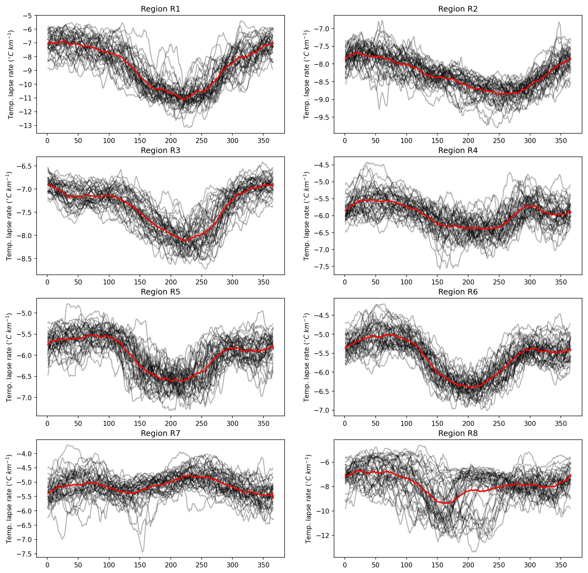
Figure A1 Annual temperature lapse rate cycles for all historical years (1980–2018, black lines) overlain with the median annual cycle (red line).

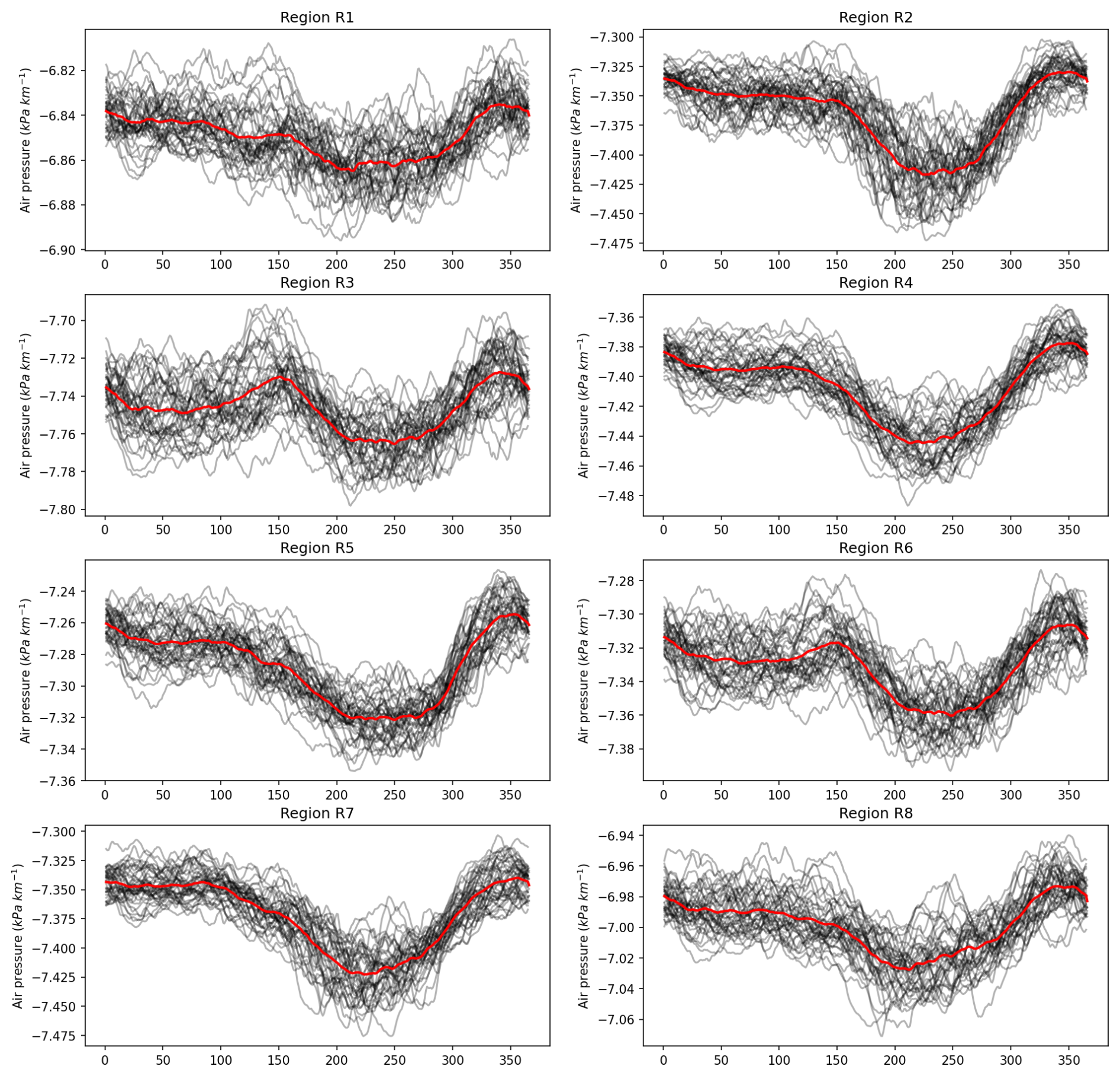
Figure A2 Annual surface pressure lapse rate cycles for all historical years (1980–2018, black lines) overlain with the median annual cycle (red line).

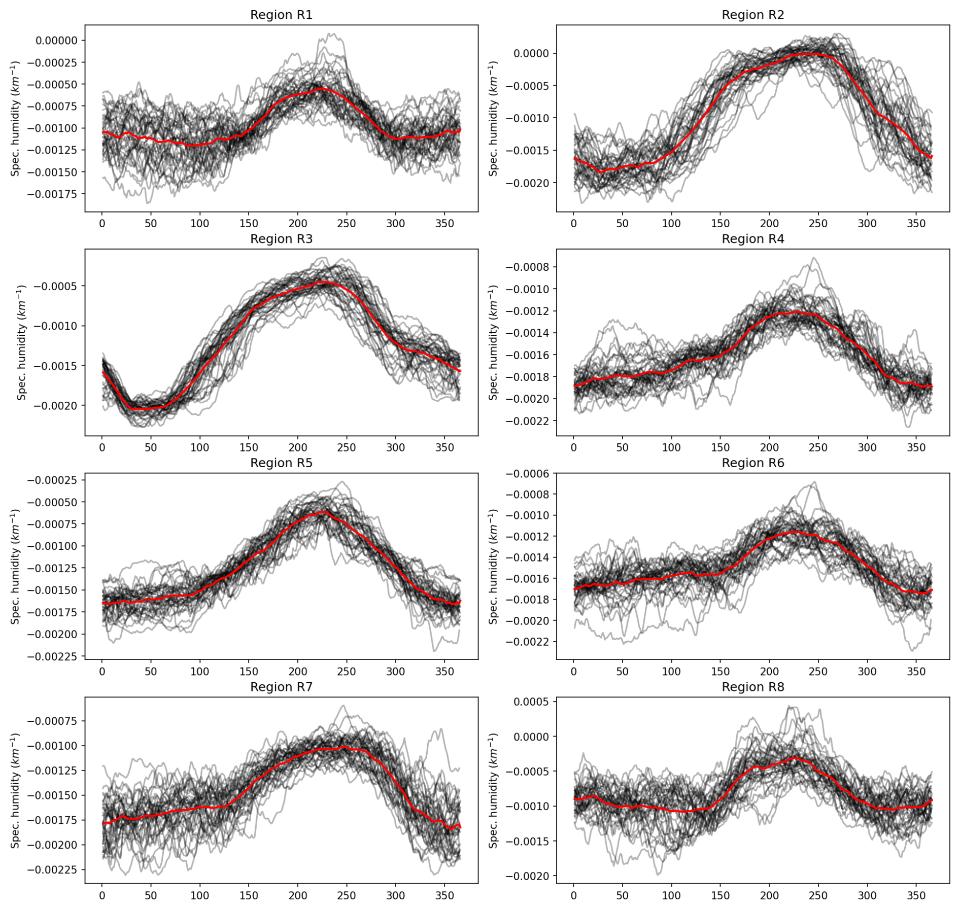
Figure A3 Annual specific-humidity lapse rate cycles for all historical years (1980–2018, black lines) overlain with the median annual cycle (red line).

Appendix B: Assessment of relationship between glacier characteristics and simulated mass balance errors

Figure B1 Comparison of simulated mass balance errors to six glacier characteristics.

Appendix C: Comparison of JULES–OGGM simulations to a subset of GlacierMIP simulations

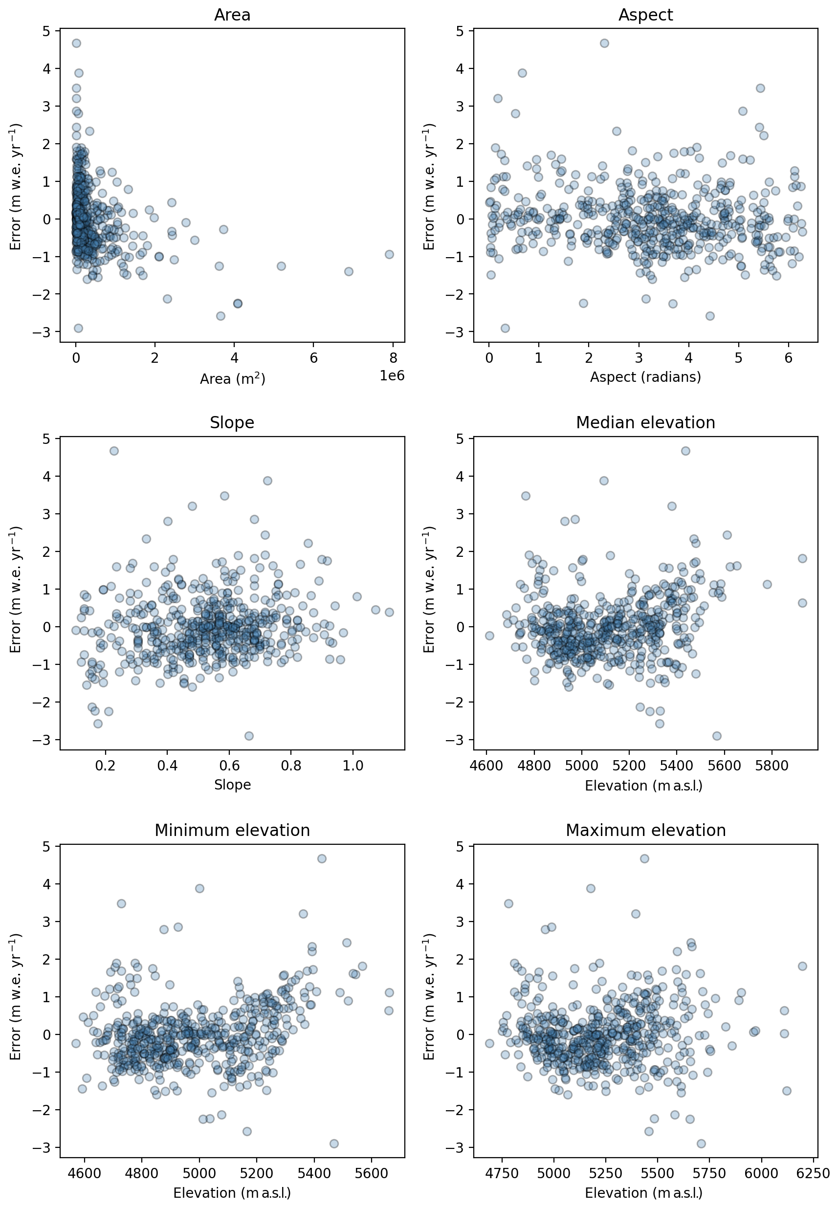
Figure C1 Simulated annual total glacier area (a, b) and mass (c, d) for the VUB between 2000 and 2100 based on RCP4.5 and RCP8.5 scenarios. Simulations include JULES–OGGM and those from the GloGEM and MAR2012 models from the GlacierMIP experiments (Marzeion et al., 2020). Solid lines represent the ensemble mean simulations using all available GCMs that are not coherent across glacier models. Dashed lines represent simulations driven with the subset GCMs that are coherent across the glacier models. Shaded areas represent the 90 % confidence bounds.

Appendix D: Selection of the BNU-ESM simulation

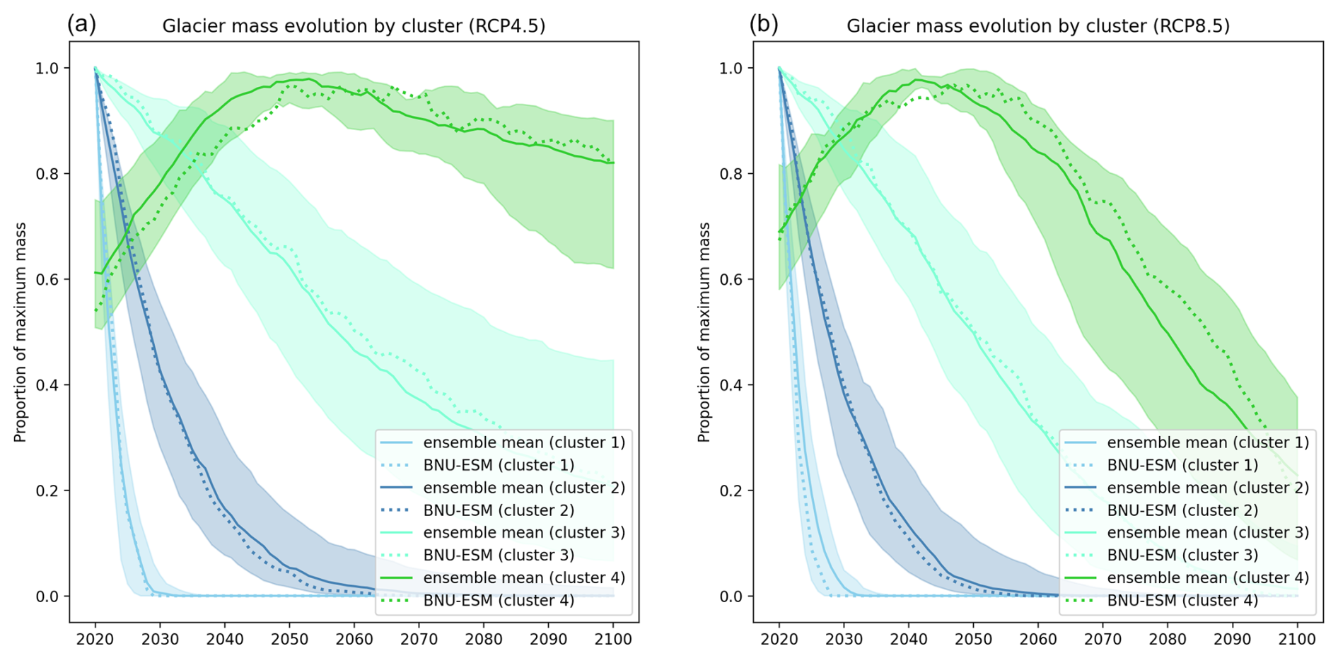
Figure D1 Annual glacier mass evolution of four identified clusters expressed as the proportion of the maximum simulated mass between 2020 and 2100 for RCP4.5 (a) and RCP8.5 (b) overlain with the BNU-ESM simulation, which was selected to most closely match the ensemble mean. Annual glacier mass evolution of four identified clusters expressed as the proportion of the maximum simulated mass between 2020 and 2100 for RCP4.5 (a) and RCP8.5 (b) taken from the ensemble mean. Each cluster is represented by the median (solid line) and interquartile range (shaded area).

Appendix E: Mass and energy balance simulations under RCP4.5

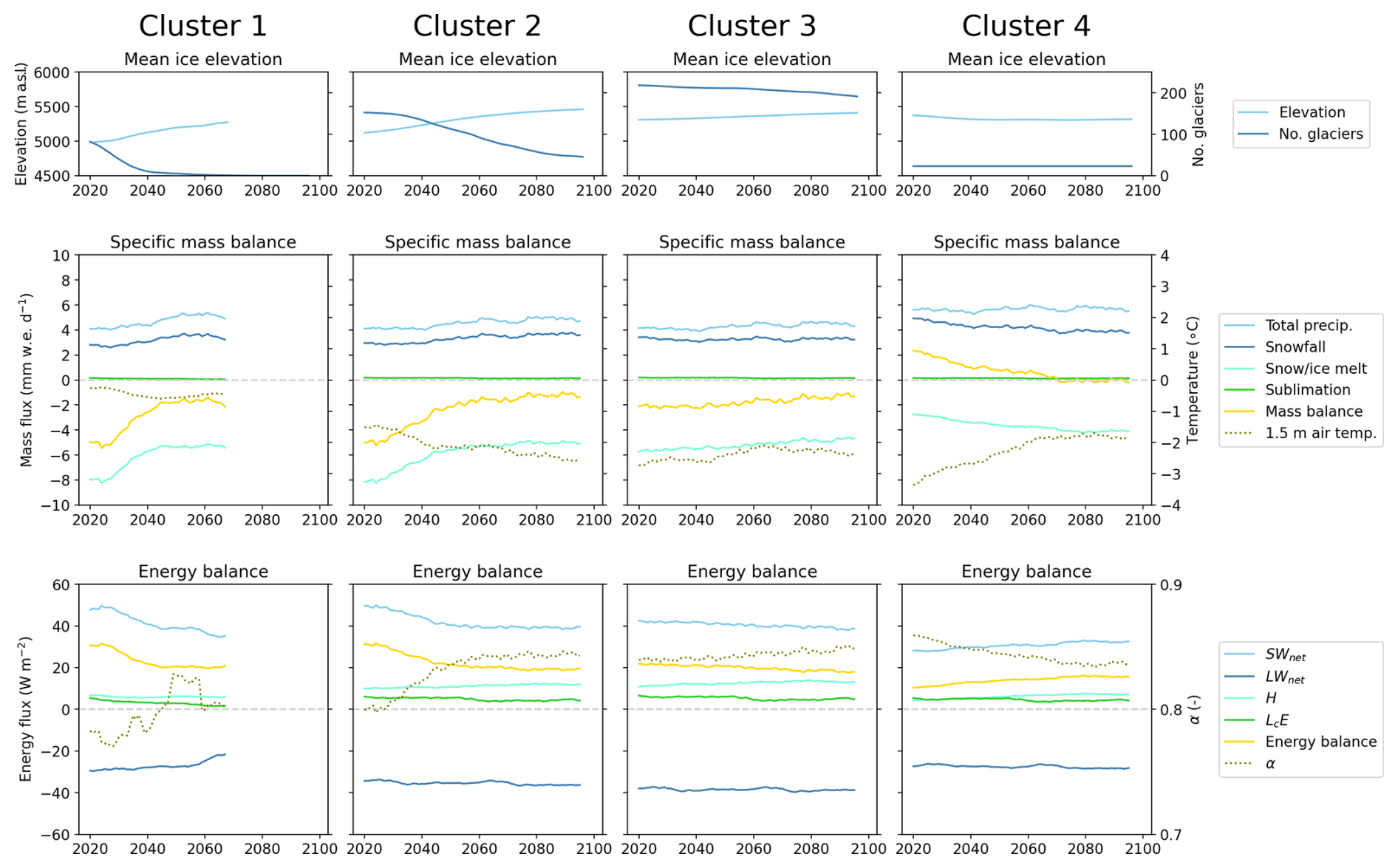
Figure E1 Simulated mean glacier-wide state variables from JULES–OGGM between 2020 and 2100 for each cluster (columns) and based on the BNU-ESM simulation under RCP4.5. The variables include ice elevation (top row), specific mass balance (middle row), and energy balance (bottom row). All variables are calculated over a 10-year moving-average window and are taken as the mean across all glaciers within a cluster as weighted by the glacier area.