Assessing uncertainties in modeling the climate of the Siberian frozen soils by contrasting CMIP6 and LS3MIP

Climate models and their land components still exhibit notable discrepancies in frozen soil simulations. Contrasting the historical runs of seven land-only models of the Land Surface, Snow, and Soil Moisture Model Intercomparison Project (LS3MIP) with their Coupled Model Intercomparison Project Phase 6 (CMIP6) counterparts allowed quantifying the contributions of the land surface parameterization scheme and the atmospheric forcing to the discrepancies. The simulation capabilities were assessed using observational data from 152 sites in Siberia and reanalysis data. In the winter months (December, January, and February), the LS3MIP ensemble bias in 0.2 m soil temperature was larger than the CMIP6 bias (−3.6 vs. −2.7 °C). The spread of winter 0.2 m soil temperatures was also larger in the LS3MIP ensemble (4.6 °C) than in the CMIP6 ensemble (3.0 °C). For permafrost sites, for all CMIP6 simulations, the correlations between winter soil temperatures with observations were below 0.6, and the correlations for spring/autumn correlations of snow depth were below 0.8. In the CMIP6 simulations, the median 0.2 m soil temperature was 0.3 °C warmer than in the observations when the simulated soil temperature dropped below −5 °C. However, the LS3MIP simulations were colder, with a cold bias in the median of 0.7 °C. The biases of 2 m temperature in coupled simulations had an opposite sign and were amplified in magnitude compared to the biases of their soil temperatures, especially below 0 °C. Our results indicate that land-only models have limited capability in reproducing soil temperatures and snow depth under severe cold conditions (surface air temperature below −15 °C). Furthermore, four climate models and their land components underestimated the insulating role of snow. In cases with shallow snow depth (0–0.2 m), the models simulated air-soil temperature differences of up to 10 °C, whereas in situ measurements indicated even larger differences. The CMIP6 models tended to compensate for errors in their land component with errors in the atmospheric model component. Therefore, to improve frozen soil modeling in climate projections, a more accurate representation of the surface-soil insulation is essential.

1 Introduction

Under current climate conditions, an amplification effect up to 2–4 times is evident in warming trends within Arctic regions compared to global averages (Rantanen et al., 2022). Specifically, from 1979 to 2018, near-surface temperature growth rates in the land area surrounding the Arctic (0.51 °C per decade) were more than 1.5 times that of the Northern Hemisphere average (0.33 °C per decade), according to Climate Research Unit (CRU) TS4.02 (Wang et al., 2022). Climate simulations indicate that the Arctic experienced a warming rate of 0.66 ± 0.32 °C per decade from 1979 to 2014 (Cai et al., 2021). Additionally, under a moderate scenario, high-latitude regions could see temperature increases ranging from 1.2 to 5.3 °C between 2005 and 2100 (Koven et al., 2013). Higher temperatures drive the degradation of permafrost, especially in discontinuous and sporadic permafrost regions. The most significant changes occur in regions where the mean annual air temperatures are around 0 °C (Romanovsky et al., 2007; Åkerman and Johansson, 2008; You et al., 2021). The soil temperature at zero annual amplitude depth of continuous permafrost sites on a global scale warmed for 0.39 ± 0.15 °C during 2007–2016. This warming is two to 3 times larger than that observed at discontinuous permafrost sites (Biskaborn et al., 2019; Smith et al., 2022), raising concerns about the potential for more substantial permafrost degradation in the future.

Large amounts of soil carbon are stored in permafrost (Tarnocai et al., 2009; Fuchs et al., 2018), and when permafrost thaws, the soil carbon could be emitted as carbon dioxide or methane into the atmosphere at a faster rate (Schädel et al., 2018). In environments such as lakes and wetlands, the impact of thawed carbon on the climate is even more pronounced due to the low-oxygen conditions, which further increase the proportion of methane emitted alongside other greenhouse gases (Koven et al., 2015; Walter Anthony et al., 2018). Processes such as thermokarst result in sudden thaw events that greatly enhance the decomposition and release of frozen soil carbon, potentially increasing carbon emissions by up to 50 % (Abbott and Jones, 2015; Turetsky et al., 2019). The winter contribution to total Arctic methane emissions is predicted to reach 39 % (Rößger et al., 2022). Permafrost thaw alters hydrothermal conditions, which can alter surface vegetation depending on soil moisture. In lowland regions with ice-rich permafrost, abrupt thawing is often followed by vegetation recovery. Under stronger or prolonged changes, the system may reach a tipping point, beyond which widespread ecosystem disruption can occur (Heijmans et al., 2022).

Despite its critical role in climate feedback processes, frozen soil remains one of the more uncertain components in Earth system models (Koven et al., 2013; Yokohata et al., 2020). In the land surface component of climate models, heat transfer through the soil is typically simulated as one-dimensional vertical transport. Models account for their specific soil layering schemes, where the thickness of soil layers generally increases with depth. By calculating the water and thermal balance at different depths, land surface models can derive the current state of soil moisture and temperature. Model parameters for hydrothermal transport are governed by soil texture, surface organic matter, moisture dynamics, and freeze-thaw conditions (Woo, 2012; Andresen et al., 2020; Yang et al., 2022). In permafrost regions, these factors determine the thermal offset (Kudryavtsev et al., 1977) – the temperature difference between the ground surface and the top of the permafrost – by altering soil hydrothermal properties. For example, the presence of solid and liquid water in frozen soil greatly affects the hydrothermal properties of the soil, which is described in various ways by different models (Niu and Yang, 2006; Li et al., 2010). Incorporating soil ice and water dynamics into land surface models improves simulations of active layer hydrothermal conditions by capturing seasonal freeze-thaw processes and moisture effects, such as summer cooling and winter warming of permafrost due to increased soil moisture (Swenson et al., 2012; Li et al., 2021; Du et al., 2023). Including soil ice dynamics in models allows for the simulation of ice-wedge degradation and associated ground subsidence, capturing rapid landscape changes such as thermokarst under strong warming scenarios (Liljedahl et al., 2016; Nitzbon et al., 2020; Cai et al., 2020). The parameterizations in land surface models are crucial for accurately representing permafrost dynamics and their associated climate feedback processes (Yokohata et al., 2020), and they also determine the inclusion of key physical and biogeochemical processes essential for modeling permafrost carbon emissions (Ekici et al., 2015; Matthes et al., 2017, 2025).

The timescales of major physical processes differ largely between the soil and the atmosphere. For instance, key variables such as temperature and humidity in the near-surface atmosphere can experience substantial fluctuations within hours or even minutes. In contrast, changes in water and thermal states within the soil become much slower as depth increases. At depths of several tens of meters beneath permafrost, soil temperatures may not exhibit any noticeable variation over decades. In this context, it is essential to recognize that the soil surface serves as a critical interface for atmospheric interactions (Beringer et al., 2001; Langer et al., 2011a, b). Snow cover plays an important role by insulating soils while affecting surface energy balance through changes to local albedo as well as other characteristics such as emissivity and roughness. The impact of snow on soil temperature exhibits spatial heterogeneity based on snow's own attributes – specifically, thickness, density, and duration (Zhang, 2005; Zhang et al., 2018). A thick snowpack provides stronger thermal insulation, which limits soil heat loss in winter and delays thawing in spring. Lower-density snow insulates more effectively due to its reduced thermal conductivity. The duration of snow cover determines the length of the insulated period, which affects the timing and amplitude of seasonal soil temperature changes. Research has shown that changes in snow conditions (snow depth, density, and duration) account for over 50 % of variations in soil temperatures observed in northeastern Siberia (Park et al., 2014, 2015). An accurate representation of snow cover is essential for climate models, as a recent study has shown significant discrepancies in snow representations across different seasonal forecasting systems over Siberia due to different snow parameterizations and initialization methods (Risto et al., 2022).

The Coupled Model Intercomparison Project Phase 6 (CMIP6), launched by the World Climate Research Program (WCRP), aims to explore various topics related to climate change (Eyring et al., 2016). It allows evaluation of the ability of the latest generation of climate models to simulate frozen soil by providing an ensemble of climate models at resolutions fine enough to distinguish different frozen soil regions. The extent and characteristics of frozen soil can vary abruptly over short distances, especially in complex terrain or transition zones between different types of permafrost. Research efforts have been conducted to improve the simulation capabilities of land surface models participating in CMIP, focusing on biological and physical processes in frozen soil areas (Ekici et al., 2014; Chadburn et al., 2015; Decharme et al., 2016; Brunke et al., 2016; Jafarov and Schaefer, 2016; Guimberteau et al., 2018; Cuntz and Haverd, 2018; Damseaux et al., 2025). The Land Surface, Snow, and Soil Moisture Model Intercomparison Project (LS3MIP) is designed to enhance our comprehension of land surface processes by assessing the effectiveness of various land-only models in simulating soil temperature and moisture, snow cover, and related hydrological dynamics. It also aims to generate valuable insights that can aid in refining land-only models (van den Hurk et al., 2016). In LS3MIP, experiments are designed so that different land-only models use the same atmospheric forcing. Therefore, LS3MIP provides an opportunity to distinguish the impact of distinct climate variabilities produced by different atmospheric models in corresponding CMIP6 models.

In CMIP6 and LS3MIP, the setup of the land cover/land use scenario and the radiative forcing conditions follow the same protocol. However, the parameterization schemes of the climate models differ, and this is considered a main source of uncertainty in climate modeling (Deng et al., 2021; de Vrese et al., 2023; Kuma et al., 2023). In addition, the presence of internal climate variability can also lead to differences in uncertainty (Ye and Messori, 2021; Rashid, 2021; Schwarzwald and Lenssen, 2022; Jain et al., 2023). Understanding and isolating these uncertainties is essential for improving model reliability.

Northern Eurasia contains more than two-thirds of the Earth's permafrost area (Groisman and Bartalev, 2007), with the majority located in Siberia. The potential degradation of permafrost in Siberia could have far-reaching consequences for climate and ecosystems throughout Eurasia and globally (Schuur et al., 2015; Streletskiy et al., 2025). Within this region, we used the soil temperature observational dataset at standardized depths, as provided by the All-Russian Scientific Research Institute of Hydrometeorological Information-World Data Center (RIHMI-WDC; Frauenfeld and Zhang, 2011; Sherstyukov, 2012a; Zhang et al., 2018).

The characteristics of frozen soil surface dynamics are assessed by comparing model outputs with references, including reanalysis and observational data. This research focuses on the shallow soil temperature response to atmospheric forcing, explicitly targeting a depth of 0.2 m. We will analyze the discrepancies between the climate models in CMIP6 and their land-only models in LS3MIP to quantify the bias and uncertainty present in frozen soil regions, attributing them to land-only models versus those resulting from atmospheric forcing. CMIP6 models include fully coupled components, such as the atmosphere, ocean, land, and sea ice, whereas LS3MIP models only include the land surface model and prescribe atmospheric forcing from reanalysis or historical simulations. As land surface models are designed to simulate the response of surface and soil parameters to prescribed atmospheric forcing, they are better constrained as driven by observation-based atmospheric conditions. Therefore, under identical observation-based atmospheric forcing, LS3MIP models are generally expected to reproduce soil conditions more accurately than their CMIP6 counterparts. If not, discrepancies may indicate limitations within the land surface models themselves, such as deficiencies in parameterization or missing processes that impair their ability to respond appropriately to atmospheric forcing. Conversely, errors found in coupled CMIP6 simulations may result from biases in atmospheric forcing, such as misrepresentation of near-surface air temperature, precipitation, or surface radiation. The experimental design of LS3MIP provides a framework that enables an evaluation of the respective contributions of these models to biases and uncertainties in soil temperature simulations within climate models. Specifically, we will explore inter-model variations within LS3MIP and assess how specific structural features, such as bottom boundary conditions and snow thermal conductivity parameterizations, relate to model performance in frozen soil regions.

2 Data and Methods

We used the data from climate models, reanalysis, observations, and processing methods of target variables for our analysis. We only included data from 1985 to 2014 in this research, as this period offers the best collection of observation records, and CMIP6 historical experiments are limited to 2014.

2.1 CMIP6 and LS3MIP Simulations

The CMIP6 multi-model ensemble provides historical climate simulations based on the same external forcing (solar radiation, greenhouse gases, aerosols, etc.) (Eyring et al., 2016). Our study used the historical simulations with predefined CO₂ concentrations, which contain distinctive combinations of atmospheric and land models. The Land-Hist experiments from LS3MIP are offline, land-only simulations with no feedback to the atmosphere and no dynamic forcing from atmospheric models (van den Hurk et al., 2016). All the LS3MIP simulations employed the same atmospheric forcing derived from the Global Soil Wetness Project Phase 3 (GSWP3) and the same land surface setup as in the CMIP6 experiments (van den Hurk et al., 2016). GSWP3 is a global land surface modeling project that provides long-term meteorological gridded forcing data based on the 20th Century Reanalysis (20CR), bias-corrected with observational datasets. This setup allowed us to directly compare CMIP6 and LS3MIP results and disentangle the relative contributions of coupling-related errors and land model deficiencies to biases in frozen soil regions.

Table 1 Selected CMIP6/LS3MIP experiment pairs, the layering and resolution. For other features and references, see Table 2.

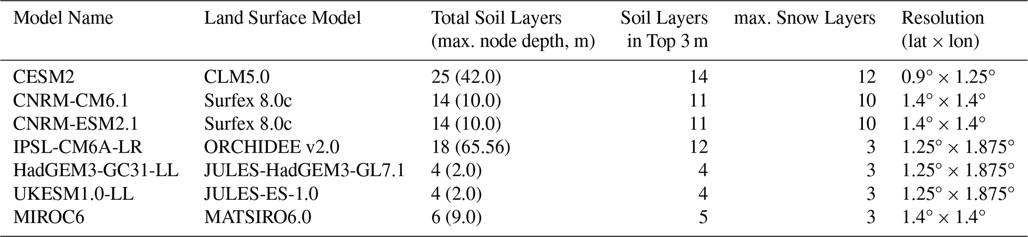
We chose seven climate models involved in both projects, incorporating six different land models. The selected models are listed in Table 1. Other climate models, which also participated in both projects, could not be included in this study as they either turned off the freeze option in frozen soil in the CMIP6 version or did not provide data for all our target variables. Hereafter, we refer to the CMIP6 as Group C and the LS3MIP as Group L in plots and analysis. Four variables are collected for this study: 2 m air temperature (tas), soil temperature in 0.2 m depth (tsl), snow depth (snd), and precipitation (pr). Both CMIP6 and LS3MIP data can be accessed at https://aims2.llnl.gov/search/cmip6 (22 May 2023).

Van Kampenhout et al. (2017)Jordan (1991)Lawrence et al. (2019)Vionnet et al. (2012)Yen (1981)Decharme et al. (2019)Wang et al. (2013)Bowring et al. (2019)Clark et al. (2011)Calonne et al. (2011)Walters et al. (2019)Wiltshire et al. (2020c)Sellar et al. (2019)Calonne et al. (2011)McNeall et al. (2024)Takata et al. (2003)Guo et al. (2021)

Table 2 Features of the land surface models. MC indicates mechanical compaction.

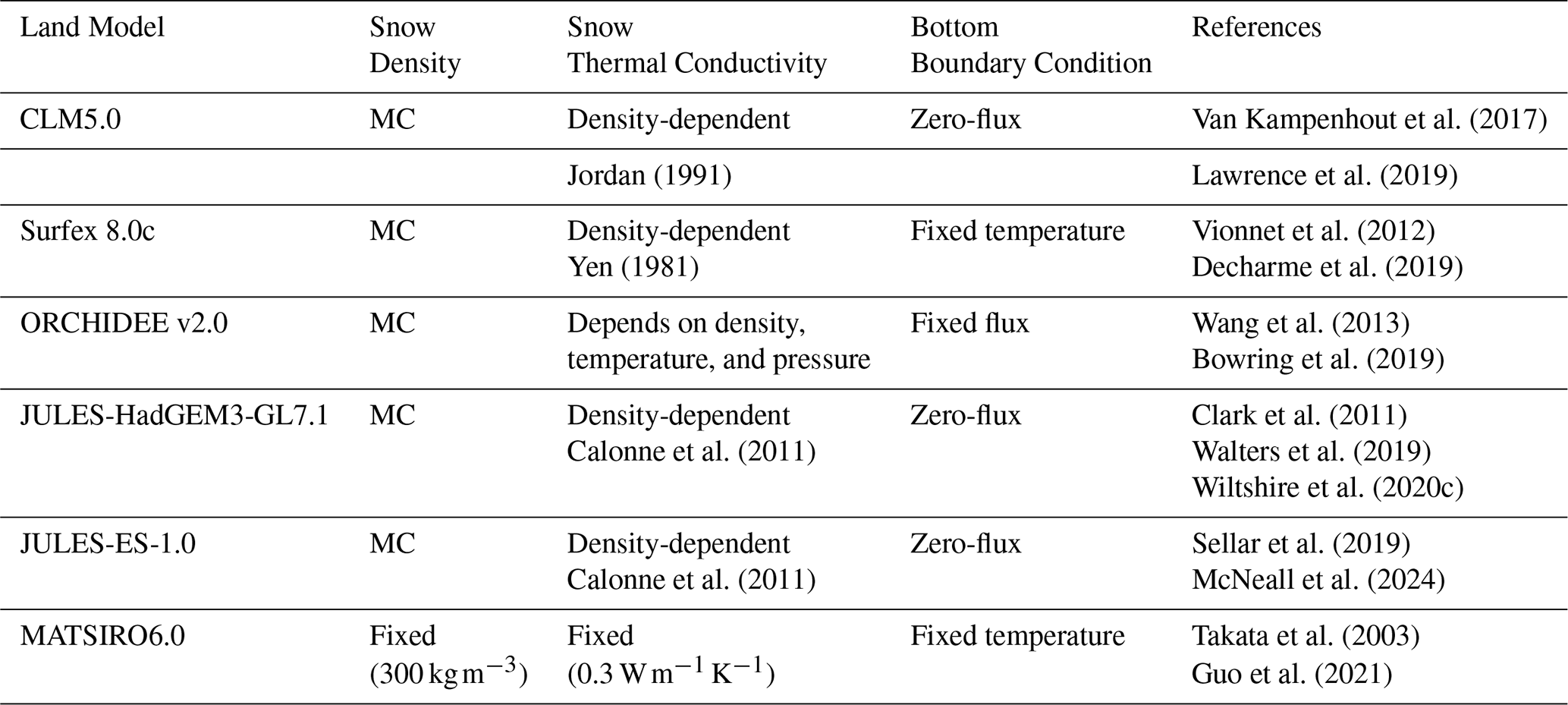
Table 2 highlights several attributes of each land model, focusing on their key characteristics related to the surface energy balance and associated processes. For a more general comparison of land-only models and their features regarding snow parameterization, see Menard et al. (2021). The land models differ in their representation of critical processes related to surface energy balance, snow physics, boundary conditions, and surface organic matter. The thermal conductivity of snow is modeled using density-dependent formulations as a power function (Yen, 1981) or a quadratic function (Jordan, 1991; Calonne et al., 2011; Wang et al., 2013), or using fixed values. Snow density is treated either dynamically through mechanical compaction (MC) or as a constant. The soil bottom boundary is handled with zero-flux assumption, fixed temperature, or fixed temperature gradients.

2.2 ERA5-Land Reanalysis

We utilized monthly averaged ERA5-Land reanalysis data from the European Centre for Medium-Range Weather Forecasts. ERA5-Land is a numerical land surface model product forced by atmospheric variables of ERA5, featuring a high horizontal resolution of 0.1° × 0.1° (Muñoz-Sabater et al., 2021; Muñoz-Sabater, 2019). Monthly data provided by ERA5-Land include 2 m temperature, snow depth, and soil temperature at four depths (0 to 0.07 m, 0.07 to 0.28 m, 0.28 to 1.0 m, 1.0 to 2.89 m). Soil temperature was linearly interpolated to a depth of 0.2 m to directly compare with observations. We also remapped ERA5-Land to a coarser horizontal resolution of 100 km (the finest resolution of the selected CMIP6 models). This remapped dataset is referred to as E5LC. Comparing ERA5-Land with its coarsened version allowed us to assess the impact of resolution on simulation outcomes. This also provided an opportunity to evaluate the reliability of ERA5-Land in representing conditions within permafrost-affected areas.

2.3 Observational Data

Observational daily data were gathered from 236 meteorology sites by RIHMI-WDC (Sherstyukov, 2012a; Bulygina et al., 2014a, b; Zhang et al., 2018). We filtered the data from 1985 to 2014 based on the quality flag (Sherstyukov, 2012b) provided in the dataset and employed only sites with a minimum of 330 valid days per year for all four target variables and at least 15 years of valid data. We only used the highest quality data, flagged as 0. Stations west of 60° E, east of 120° E, and south of 45° N were excluded to eliminate most stations with warmer climates. Moreover, sites were classified based on their winter 2 m air temperature. These criteria were put in place to ensure the accuracy and reliability of the data analyzed. A total of 152 stations were selected.

2.4 Data Preprocessing

We interpolated tas, tsl, pr, and snd for all model simulations at the station sites' coordinates by choosing the nearest-neighbor grid cell values. This introduced additional, but small uncertainty when comparing modeled data with observed data as will be shown below. In time dimension, we considered only 30 year monthly averaged data for evaluations aiming to minimize uncertainties due to climate variability and phase shifts in CMIP6 simulations.

2.5 Evaluation Metrics

To evaluate the models, we quantified their ability to simulate a reasonable climate mean state and internal climate variability.

The variability of target variables was quantified using the interquartile range (IQR), which measures the spread of the simulations. If the model over- or underestimated the observed IQR_o, the model over- or underestimated climate variability, respectively. Thus, we used the relative spread

$$\begin{array}{}\text{(1)}& {\text{RS}}_{\mathrm{m},i}={\displaystyle \frac{{\text{IQR}}_{\mathrm{m},i}}{{\text{IQR}}_{\mathrm{o},i}}}\end{array}$$

with m indicating the model, o the observation, and i the target variable.

The central climate state of the models and the observations were quantified by the median (med). We used the standardized model medians med_m,i, naming it relative bias RB,

$$\begin{array}{}\text{(2)}& {\text{RB}}_{\mathrm{m},i}={\displaystyle \frac{{\text{med}}_{\mathrm{m},i}-{\text{med}}_{\mathrm{o},i}}{{\text{IQR}}_{\mathrm{o},i}}}\end{array}$$

as a measure of systematic model errors.

RS assesses a model's capability to reproduce the observed variability. This is essential for determining a model's reliability in simulating dynamic climate systems.RB, on the other hand, addresses systematic deviations using the median data values. It was standardized using observed variability (IQR_o), which facilitates comparisons of biases across different variables. RB emphasizes whether systematic errors are pronounced relative to natural variability (informs if the error is smaller (${\text{RB}}_{\mathrm{m},i}<\mathrm{1}$) or larger (> 1) compared to the observed climate variability), helping prioritize improvements in model development.

For the quantification of the error heterogeneity of the 2 multi-model ensembles at the sites' locations, we defined the ensemble means of the models' 30 year median biases as follows

$$\begin{array}{}\text{(3)}& {\text{EB}}_{i,\mathrm{s}}=\sum _{m=\mathrm{1}}^{\mathrm{M}}{\displaystyle \frac{\mathrm{1}}{F{N}_{\mathrm{m}}}}({\text{med}}_{\mathrm{m},i,\mathrm{s}}-{\text{med}}_{\mathrm{o},i,\mathrm{s}})\end{array}$$

where s indicates the seasons, F=5 represents the number of “model families” and N_m, which represents the number of “family members” (either 1 or 2 in this study), was used to properly weight similar models, as described in Kuma et al. (2023). We then calculated the ensemble spreads of median biases ES_i,s, which were defined as the standard deviations.

The ensemble mean biases EB_i,s and spreads were calculated for both the CMIP6 and LS3MIP model ensembles with M=7 members each. The analyses were done in different seasons to distinguish the impact of different freeze/thaw periods on ensemble performance. In this study, seasons were defined by months. Winter was defined as December, January, and February (DJF); spring as March, April, and May (MAM); summer as June, July, and August (JJA); and autumn as September, October, and November (SON).

The simulation performance at specified sites was quantified using Taylor diagrams (Taylor, 2001). The data were compared with observations across all seasons in the permafrost region. The correlation coefficient was computed from two-dimensional data (19 stations × 3 months), thereby reflecting the agreement between the model and observations in both spatial distribution and sub-seasonal variation.

We applied additional statistical analysis to the temperature variables of CMIP6 and LS3MIP ensembles, focusing on temperature states, including interquartiles, medians, means, standard deviations, and kurtosis. The kurtosis characterizes the shape of a distribution, where a value of 0 indicates a normal distribution. When the standard deviations are comparable, a higher kurtosis indicates a distribution with heavier tails, i.e., more extreme deviations from the mean.

2.6 Categorization of Stations

We aimed to assess the models' performance under different climate conditions to determine whether simulation uncertainties increase at lower temperatures or remain similar. To distinguish between different climate regimes, one possible approach is to categorize stations based on their average DJF 2 m air temperature (Wang et al., 2016).

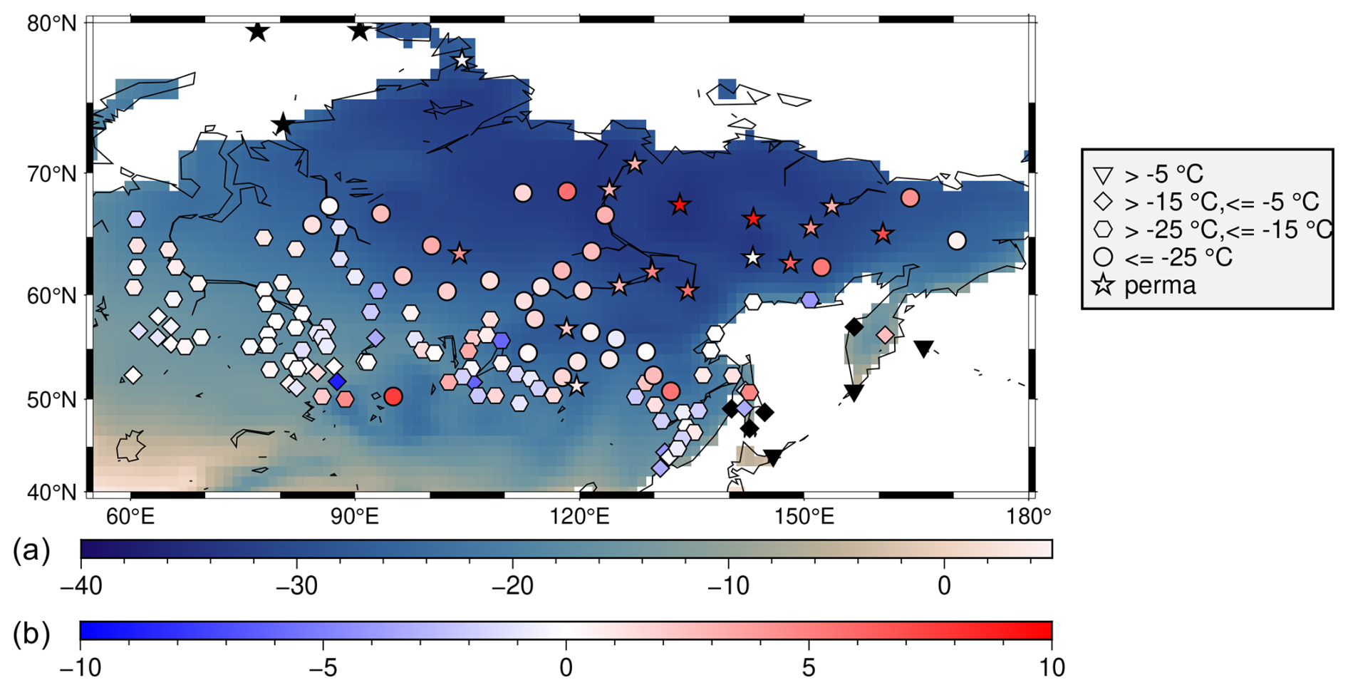
Figure 1 Mean near-surface air temperature (a) as given by the weighted multi-model ensemble from CMIP6, and the difference between the ensemble mean and the observational data (b) at sites for winter (DJF) in 1985–2014 in °C. Symbols indicate the climate state at the observational sites (see legend), and symbol colors show the difference between the ensemble mean and the observational data.

We expanded the scope by focusing on air temperatures when snow is present, not just during the DJF period, and linked the results to the insulating effect of snow. To investigate the climatology in the permafrost area, sites were further identified as valid permafrost sites using the definition of Lawrence and Slater (2005). If a station had at least 300 d of valid data every year and 24 consecutive months of lower than 0 °C in any layer below 0.2 m depth, it was defined as a valid permafrost station. Using this method, we selected 19 valid permafrost stations among all observation sites.

3 Results

3.1 Winter 2 m Temperature in Target Area

Figure 1 shows the map of average winter (DJF from 1985 to 2014) 2 m air temperatures (tas) from the CMIP6 multi-model ensemble, and the symbols correspond to the observation data from RIHMI-WDC. As shown in the map, winter-time tas in the target area is colder in the northeast and warmer in the southwest. Within the area north of 45° N and from 50 to 185° E, the average DJF tas is generally below 0 °C. The region colder than −25 °C had a large overlap with the continuous permafrost region (Brown et al., 1997; Obu et al., 2019).

The temperature categories were listed in the legend of Fig. 1. There were 3 sites with average tas warmer than −5 °C, 25 sites between −15 and −5 °C, 76 sites between −25 and −15 °C, and 29 stations with tas below −25 °C. Besides, 19 sites were identified as valid permafrost (“perma”) sites using the method introduced by Lawrence and Slater (2005) (soil layer temperatures continuously below 0 °C for at least two years) and labeled by stars. All “perma” sites had average winter tas values below −23 °C.

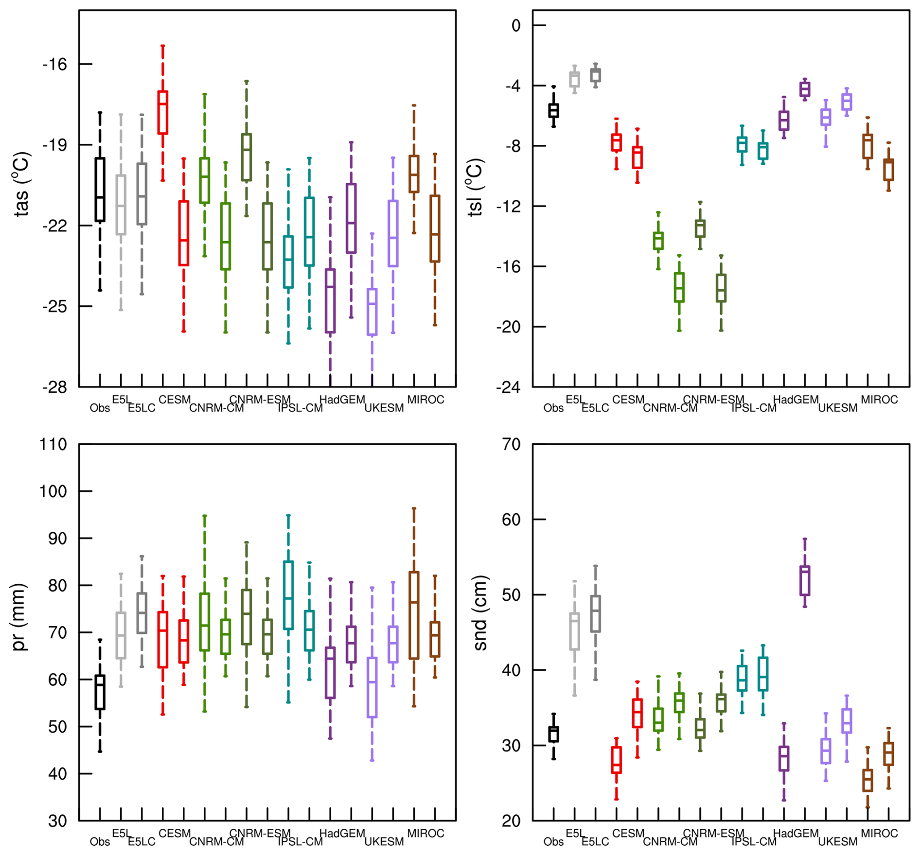
Figure 2 Sites' averaged DJF-climates (1985–2014) of hydrothermal variables as observed and simulated. Names on the x-axis and the colors indicate the different data sources. In addition to observations, ERA5-Land (E5L) and its coarsened variant, E5LC, are included to enable comparison at the same horizontal resolution as CMIP6 and LS3MIP. Model names indicate CMIP6 model output (left), and LS3MIP (right; see Table 1). Each CMIP6-LS3MIP pair shares the same color. The boxes represent the medians, first and third quartiles; the ± 1.5 × IQR or the maximum and minimum values, if within the former range, are taken as the whiskers' length.

3.2 Model Climatologies

The sites' averaged winter climatologies (DJF) of the four target variables for the different datasets from 1985 to 2014 are shown in Fig. 2. All model variables were interpolated into the site's locations using the nearest neighbor method.

ERA5-Land's tas and tsl climatologies are closer to the observed climatologies than those of most models, though this is not the case for pr and snd. Both ERA5-Land and E5LC were interpolated into the sites' locations using the nearest neighbor method. Although the coarser resolution yielded slightly higher values for the four analyzed variables, the median differences between ERA5-Land and E5LC were all smaller than one interquartile range of the observations.

In LS3MIP, tas and pr were derived from the same forcing data. However, Fig. 2 shows slight discrepancies of tas (less than 1 °C) and pr (less than 3 mm) among land-only models. The LS3MIPs' tas climatologies were systematically colder by more than 1 °C than observations and E5LC, and their pr climatologies aligned better with E5LC than with observations (which have on average about 15 % smaller values).

The CMIP6 models' tas climatologies scattered substantially. CESM2's tas median was shifted by more than +3 °C against observations, while tas medians of HadGEM3-GC31-LL and UKESM1.0-LL were shifted by more than −3 °C.

Most models' tsl climatologies were colder than observed. The CNRM simulations exhibited the lowest soil temperatures overall (Fig. 2) with the climatologies of being more than 8 °C lower in both CMIP6 and LS3MIP. The strong cold bias of CNRM-CM6.1 and CNRM-ESM2.1 is also shown during spring and autumn (Fig. A3). As expected, the temporal variability, quantified by the box plots' IQR, was smaller in tsl than in tas. Substantial inter-model variability was observed in soil temperature simulations. The differences between a model's CMIP6 and LS3MIP tsl were much smaller than their differences from observations. Land-only models that belong to the same family (the land components of two CNRM models and the models HadGEM and UKESM, see Table 1) exhibited similarities in tsl medians and IQRs.

In the other seasons, the spread of tas and tsl climatologies was, respectively smaller than in DJF. During JJA (Fig. A1), model differences in tas variability were clearly reflected in tsl, particularly as snow was absent at most sites during summer (median value less than 0.3 cm).

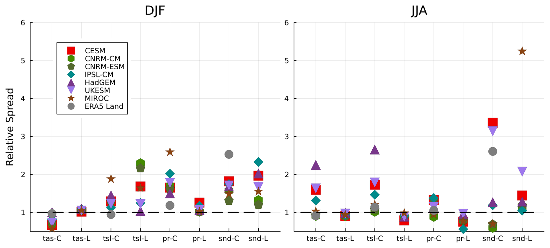
Figure 3 Relative spread (RS) of the sites-averaged climates (1985–2014) of the four variables in both ensembles and in E5LC with reference observations for DJF and JJA. The colors indicate the models, and the x-axes show the variables and ensembles (C indicates CMIP6, and L indicates LS3MIP runs).

In both CMIP6 and LS3MIP runs, the DJF pr values were typically 10 mm higher than in the observations. UKESM1.0-LL simulated relatively good pr in CMIP6, with less than 3 mm overestimation in DJF average. The observed DJF snd was approximately 30 cm. It was overestimated by 70 % in HadGEM3-GC31-LL (LS3MIP run) and by 50 % in E5LC. Overall, the models were diverse in simulating DJF medians snd, with high temporal variability.

3.2.1 Relative Spread and Relative Bias

This subsection compares the relative spread (RS) and relative biases (RB) of E5LC and the different models compared to observations for all four target variables and all seasons. The RS assesses the sites-averaged temporal climate variability, and RB is the shift of the climatologies.

Most CMIP6 models underestimated tas DJF climate variability and overestimated tsl climate variability (Fig. 3). The LS3MIP models showed an even larger tsl diversity in winter, ranging from 1 to almost 2.7, but performed better in simulating JJA variability of tsl, though with a general underestimation. In DJF and SON, the tas RS for all CMIP6 models were within the range of 0.5 to 1. In MAM, they were within the range of 0.7 to 1.7. CESM2, HadGEM3-GC31-LL, and UKESM1.0-LL exceeded 1.5 RS of tas in JJA. Larger variability differences in simulated tsl were observed for LS3MIP simulations in DJF and SON, even though their tas share almost identical RS.

The DJF pr relative spreads of CMIP6 models were all higher than 1.3. In spring and autumn, most climate models simulated good interannual variability of pr, with less than a 20 % difference to observation (Fig. A2). Both groups and E5LC overestimated the snd spread in DJF with large inter-model discrepancies. The RS of snd scatter between 0.8 and 1.8 in SON, and 1 and 1.6 in MAM for most models (except for E5LC, CNRM-CM and MIROC in CMIP6, and HadGEM in LS3MIP).

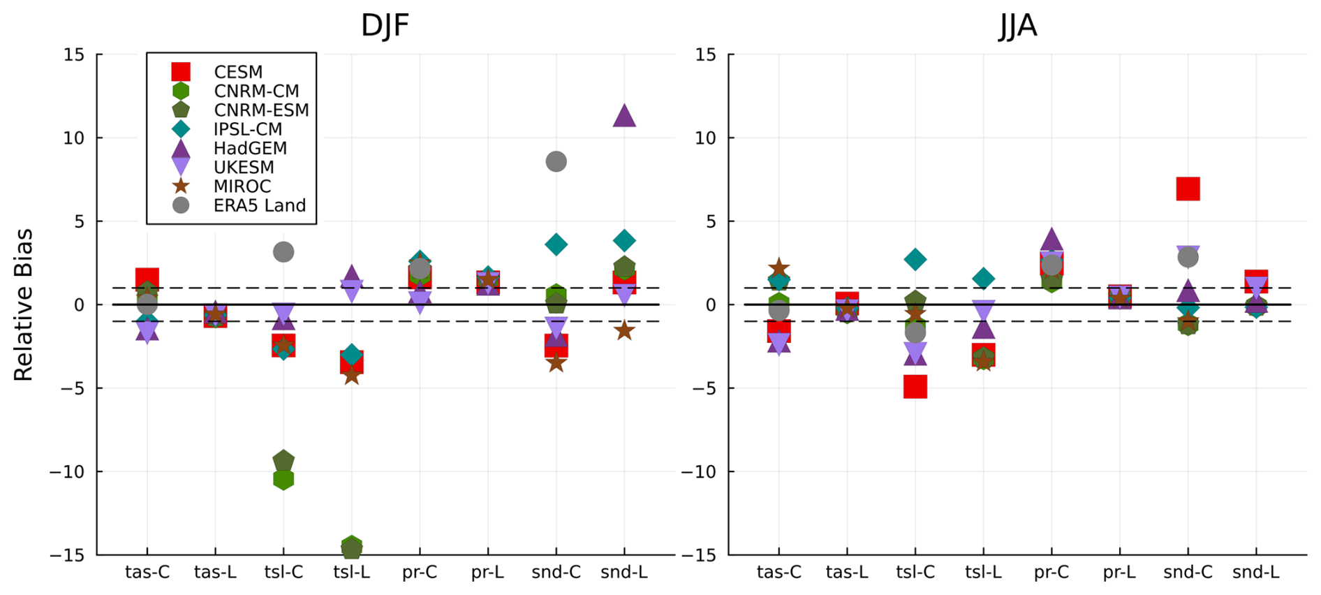
Figure 4 Same as in Fig. 3, but for relative biases (RB). The dashed lines indicate the range of absolute median differences smaller than the observation's IQR.

The relative bias RB of all variables calculated in all seasons is shown in Fig. 4. If a model's absolute RB is less than one, its performance is considered adequate. For example, the winter RB of all LS3MIP models was within the dashed line zone in Fig. 4 for tas, and at or slightly above 1 for the DJF pr as they are derived from the same atmospheric forcing data. All CMIP6 and LS3MIP models exhibited a positive relative pr bias. The relative snd bias was much more diverse; models only showed a consistent positive snd bias in MAM (Fig. A3). The CMIP6 runs of HadGEM3-GC31-LL and UKESM1.0-LL underestimated the values of tas and tsl in all seasons. The tsl RB in DJF for CNRM simulations exceeded −15 to −9 times the observed IQR, while other models were all within a range of ± 5 times in both groups. The RB of CMIP6 and LS3MIP in tsl were all negative in the transition seasons (Fig. A3), and also high discrepancies were shown in snd RB values.

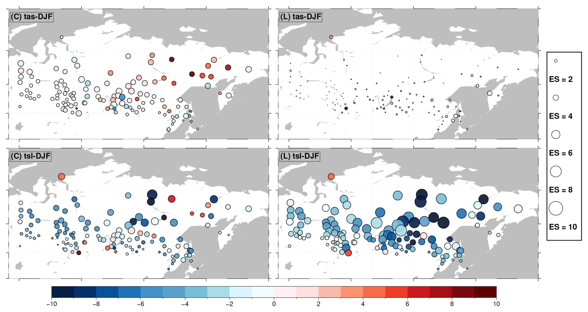
Figure 5 Weighted DJF multi-model mean biases (EB) and their standard deviations (ES) of tas and tsl at observational sites in °C. The top-left subtitles of each subplot indicate the presented model ensemble (C for CMIP6 and L for LS3MIP), the variable, and the season. Colors indicate the bias value (in °C), while the circle radii represent biases' standard deviations (in °C), i.e., the ensemble spread.

3.2.2 Spatial Heterogeneity

In DJF, the multi-model ensembles exhibited the largest EB and ES (Fig. 5). On average, the CMIP6 models overestimated tas by more than 0.5 °C, with a large ES of 3.0 °C, while LS3MIP showed a mean EB of −0.5 °C and a smaller ES of 0.7 °C. CMIP6 models tended to produce warm tas biases, whereas LS3MIP land models exhibited cold tsl biases at the same locations, particularly in Siberia.

In the other seasons (Fig. A4), EB and ES were distinctly smaller, with most CMIP6 runs' tas slightly too cold in spring at most stations and slightly too warm in autumn in northeastern Siberia. The tas EB of the forced models was small at most sites (exceptions were near water bodies, e.g., Lake Baikal and sea coasts, which indicated interpolation artifacts due to the selected grids).

The tsl EB and ES were larger in magnitude than for tas, especially in winter, with spatial averaged EB of −2.7 and −3.6 °C for CMIP6 and LS3MIP runs, respectively. Additionally, the LS3MIP runs had a larger bias spread than the CMIP6 runs in all seasons except summer. In winter, the ES were 3.0 °C for the CMIP6 and as large as 4.6 °C for the LS3MIP runs.

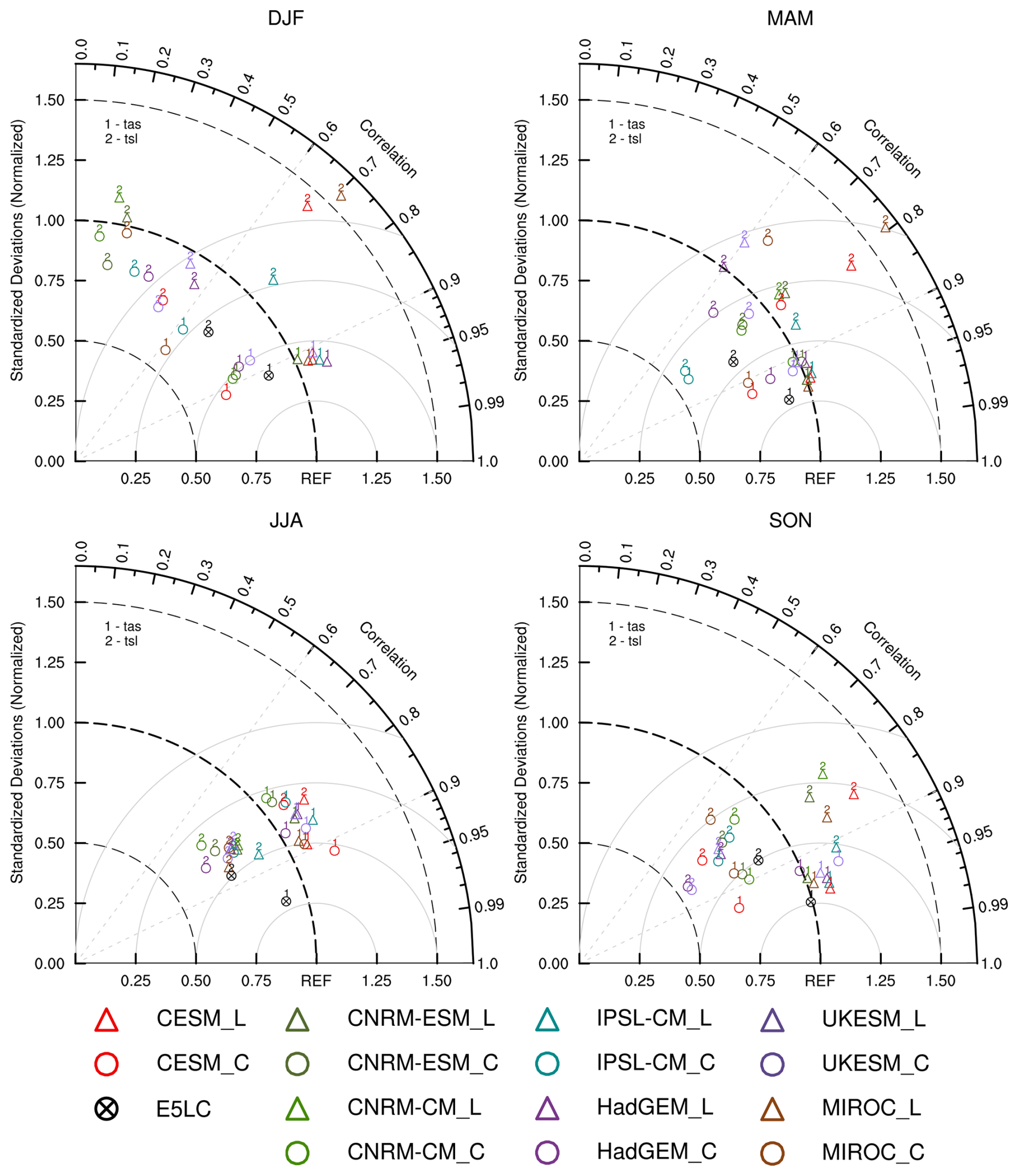
Figure 6 Taylor diagrams indicating the correlation, normalized standard deviation, and unbiased root-mean-square (RMS) difference (gray circles) for the four seasons of the simulated variables tas, tsl (labeled by numbers) against observations (REF) at valid permafrost sites (here: sites with mean winter tas < −25 °C). Normalization is applied using the standard deviations of the observations. The correlation used in this figure is the Pearson correlation coefficient. Colors indicate different models, and black crossed circles indicate E5LC. Triangles show the results of the LS3MIP runs, and solid circles of the CMIP6 runs. The REF indicates the corresponding observation.

3.3 Permafrost Region

Using the classic definition of permafrost, which requires more than two consecutive years of temperatures below 0 °C, we categorized 19 valid permafrost sites (see Sect. 2.6). Notice that in the permafrost region, the largest EB and ES are shown (see Fig. 5).

In JJA, both ensembles showed a high correlation with the observations (higher than 0.7). Both ensembles simulated JJA tas within a normalized standard deviation ranging from 1.00 to 1.20, while E5LC's normalized standard deviation was lower than 0.95. In the other seasons, the tas simulations had correlations higher than 0.6; however, most CMIP6 models underestimated the normalized standard deviation of tas. In MAM and SON, tas correlations were all above 0.85, which was slightly higher than tas correlations in JJA.

Almost all CMIP6 and LS3MIP models struggled to simulate tsl at valid permafrost sites, exhibiting low correlations and large RMSE, especially during DJF. The correlations were generally higher than 0.6 for both temperature variables in the other seasons. E5LC had similar DJF tas simulation performance as the CMIP6 models, but it simulated DJF tsl with the smallest RMSE of all models. For model pairs from CMIP6 and LS3MIP, the land-only simulations consistently showed higher DJF tsl correlations than the corresponding coupled simulations.

From spring to autumn, the CMIP6 models tended to overestimate precipitation variability (see Fig. A5). Overall, the LS3MIP models and E5LC showed higher correlations than the CMIP6 models in the MAM and SON snd simulations. In MAM, the normalized standard deviation of LS3MIP snd was considerably larger than in DJF and SON, generally exceeding 1.25 times the reference value. Using the same forcing, the snd correlations improved from autumn to spring, with all values above 0.8 except for UKESM1.0-LL, which had a correlation around 0.7 in SON and MAM. The correlations of CMIP6 pr were similarly lower than 0.9 from autumn to spring. LS3MIP showed a high correlation (higher than 0.85) and a stable normalized standard deviation (1.25 to 1.50) for pr in SON, DJF, and MAM. Most LS3MIP models were able to simulate snd correlations higher than 0.8 in these seasons.

3.4 Climate Dependency of Modeled Temperatures

Larger model biases and discrepancies were found in permafrost regions. To evaluate how model errors depend on the temperature conditions, we categorized all the model outputs of tas and tsl based on their values and compared these outputs to the corresponding observations. For each model, the monthly data from every site was calculated as an average over 30 years. We then examined the corresponding values for the same site and month with valid observations, calculating the median values, quartiles, and deciles for each interval.

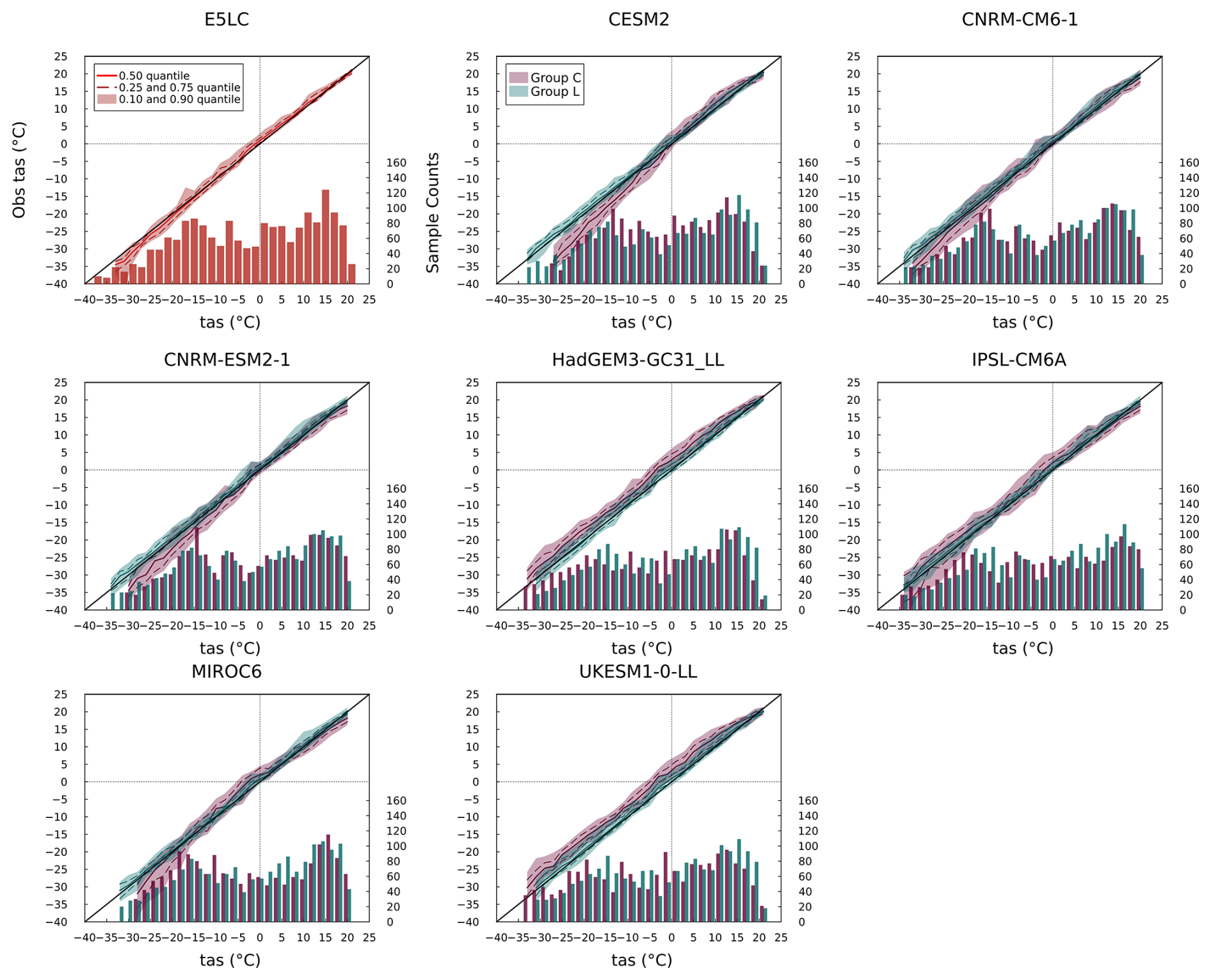
Figure 7 Quantile-Quantile (Q-Q) and histogram plots (Wilks, 2019) for tas. The plots show 30 year mean monthly tas data of models at all sites and their observational values. The model simulations are binned into 2 °C intervals. Each bar (or pair of bars for CMIP6 and LS3MIP) is plotted at the center of its interval (e.g., 1 °C for 0 to 2 °C). The solid and dashed colored curves represent the median and $\mathrm{1}\mathrm{st}/\mathrm{3}\mathrm{rd}$ quartiles, respectively, of the corresponding observations for all data points within the temperature interval. The shaded area indicates the interdecile range. The histograms represent the sample size within each temperature interval, and temperature intervals with sample sizes smaller than 20 are excluded from the Q-Q plots. The further away the data is from the diagonal line, the larger the model's simulation bias is at certain temperature states. A higher vertical quantile range indicates more inconsistency with observation under identical temperature conditions.

As shown in Fig. 7, LS3MIP models generally reproduced the observed sample distribution of tas and maintained narrow quantile spreads across the full temperature range. In contrast, CMIP6 models exhibited larger deviations. For example, CESM2, CNRM-CM6.1, and CNRM-ESM2.1 tended to simulate tas higher than observed when the observed tas was below 0 °C, with median differences exceeding +3 °C. HadGEM3-GC31-LL and UKESM1.0-LL, by contrast, consistently produced tas values approximately 5 °C lower than observed across a broad range of frozen conditions. IPSL-CM6A-LR showed persistent cold biases of over −5 °C in most subzero-temperature cases. MIROC6 produced tas values that were lower than the observed values between −10 and 2 °C, but the simulated tas values were increasingly higher than the observed values when simulated tas dropped below −20 °C. A common feature of CMIP6 models was a wider spread of quantiles in the below-freezing temperature range, especially when tas dropped below −15 °C.

Figure 8 Same as Fig. 7, but for tsl.

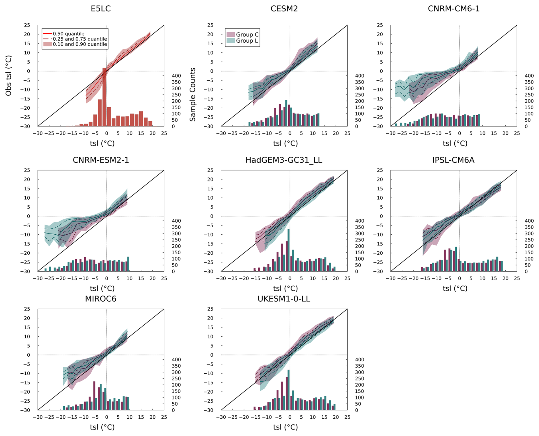
Compared to tas, quantile spreads were generally larger in the tsl simulations. For instance, the E5LC model exhibited a bimodal tas sample distribution (Fig. 7), with one peak near 15 °C and another around −15 °C, whereas its tsl sample distribution (Fig. 8) showed a single dominant peak between −5 and 2 °C. E5LC also displayed smaller and more centered tsl quantiles above 0 °C, but it showed an increasing warm bias and quantile spread as tsl dropped below freezing. Similar near-surface soil warming was observed in the LS3MIP run of HadGEM3-GC31-LL, which was associated with excessive snow depth. CNRM-CM6.1 and CNRM-ESM2.1 were the only models that did not show a cluster of tsl values near 0 °C. Instead, their tsl sample distributions were shifted toward much lower values (with extreme values lower than −15 °C), showing median differences from observations reaching −17 °C. CESM2 and MIROC6 also displayed systematic cold biases, with median tsl differences of −5 and −6 °C, respectively, when the observed tsl was around −10 °C. LS3MIP models varied more in magnitude but generally showed positive tsl biases below 0 °C.

The two groups also showed distinct differences in simulating cold temperature extremes, particularly in the minimum tas. For example, CESM2's minimum tas in the coupled simulation was 6 °C higher than in its land-only simulation, indicating a notable warm bias in the coupled system at the lower extreme. In contrast, HadGEM3-GC31-LL and UKESM1.0-LL simulated minimum tas values that were 2 °C lower in the coupled runs than in their land-only counterparts. These discrepancies in tas at the cold end of the sample distribution were also reflected in the tsl simulations. In particular, the minimum tsl values differed by up to ± 6 °C between models in the two groups.

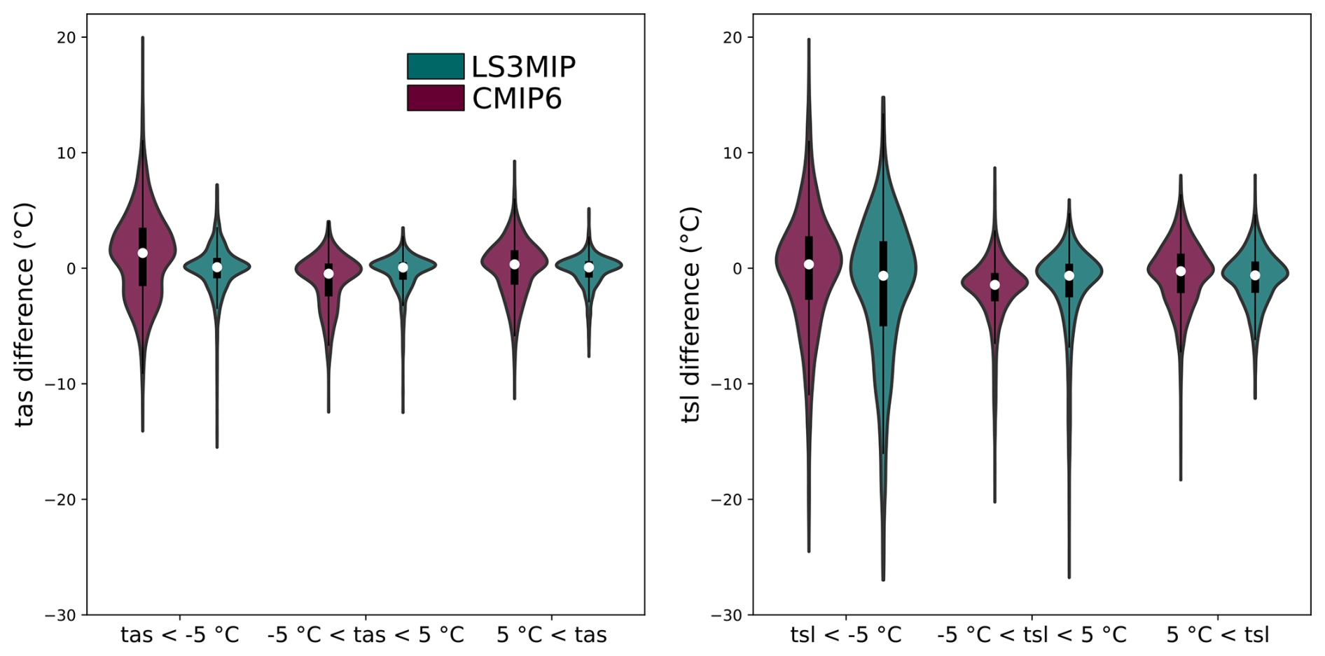
Figure 9 Difference between model tas (left), tsl (right) and corresponding observations. The x-axis represents different temperature intervals, and the y-axis is the 30 year average temperature difference (T_model−T_obs). Differences are categorized into three sets according to the 30 year average temperatures of every month at the observation sites: below −5 °C (Set Frozen), −5 to 5 °C (Set Intermediate), and above 5 °C (Set Warm). The violin plots show the distribution of the data. The width represents the density of the data points. The white dots show the median values, and the thick vertical black lines show the interquartile range.

We subtracted the 30 year average of monthly observational data from all stations with the corresponding simulated values and then sorted them into observed temperature intervals, as shown in Fig. 9. The boundary of −5 and 5 °C was chosen to make sure the soil is completely frozen/thawed in the Set Frozen/Set Warm.

Table 3 Statistics of the differences between the weighted multi-model ensembles and the observations of tas and tsl, as illustrated in Fig. 9. Here, kurtosis refers to excess kurtosis, which is kurtosis minus three.

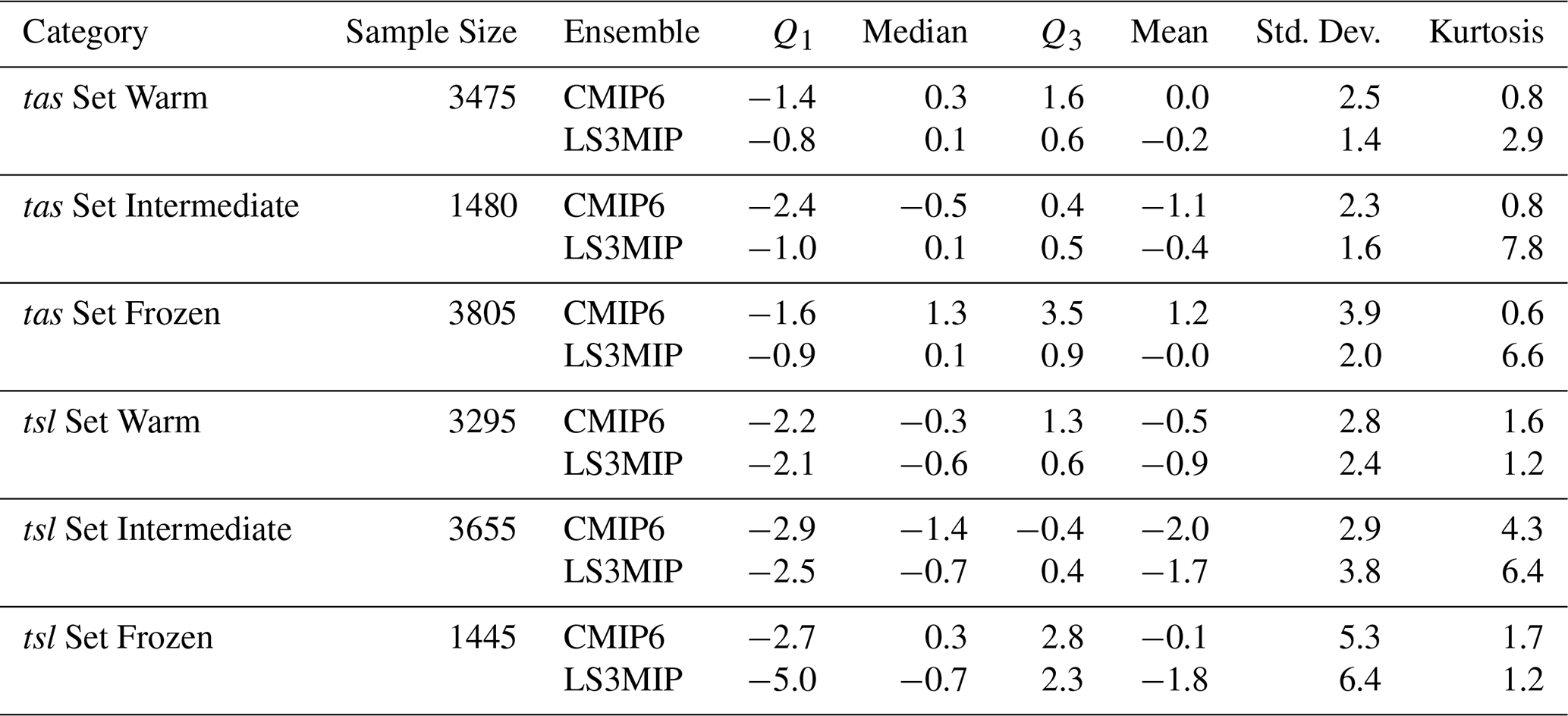
Statistical values of Fig. 9 were listed in Table 3. Set Frozen and Set Warm tas data sample sizes were more than twice as large as in Set Intermediate. Set Frozen had the largest standard deviations, 3.9 °C in CMIP6 runs, and 2.1 °C in LS3MIP runs. The mean tas values of the CMIP6 runs ranged from −1.1 and 1.2 °C. CMIP6 shows tas kurtosis from 0.6 to 0.8 in all three Sets. LS3MIP shows higher kurtosis, especially in Set Intermediate and Set Frozen (7.8 and 6.6, respectively).

The tsl samples were mainly concentrated in Set Intermediate and Set Warm. In contrast, there were also higher standard deviations in Set Frozen, 5.3 and 6.4 °C for CMIP6 and LS3MIP runs, respectively. The standard deviations of Set Frozen and Set Intermediate in LS3MIP runs were higher than those in CMIP6 runs by 1.2 and 0.9 °C, respectively. The mean and minimum values of tsl bias were much lower than those of tas bias, and this negative bias was shown in all corresponding sets of both groups in Table 3. And tsl below −5 °C showed higher overall variability in LS3MIP than in CMIP6, with the highest IQR of 7.4 °C, and the highest standard deviation of 6.4 °C among all categories. The kurtosis values of the two ensembles are more similar in tsl than in tas.

3.5 Snow Insulation

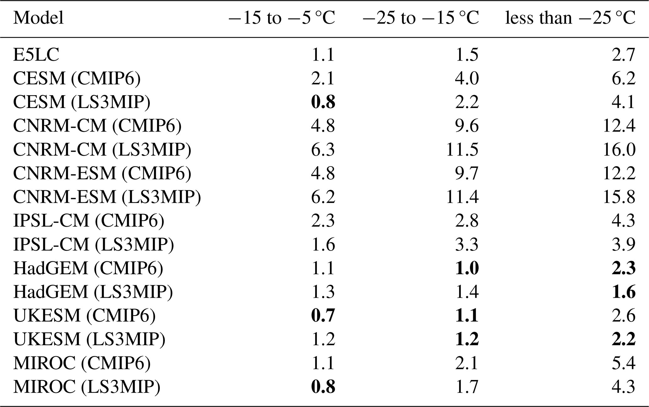
To better understand the insulating effect of snow in the models, we applied a method similar to that used in previous model evaluations (Wang et al., 2016; Burke et al., 2020). We collected the monthly observational data samples containing tas, tsl and snd and characterized them by three different tas intervals (−15 to −5 °C, −25 to −15 °C, and less than −25 °C). Analyzing the relationship between the temperature difference ΔT = tsl−tas and snow depth allowed us to understand each model's snow insulation effect under different tas and snd conditions.

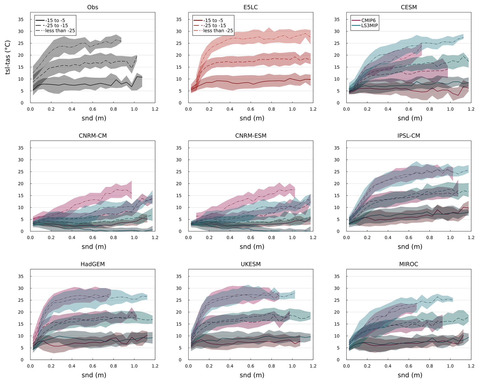
Figure 10 Snow depth and soil-surface temperature differences. The temperature categorization method follows Wang et al. (2016) but includes data from all seasons. The plots use different line styles and color schemes to distinguish between different temperature (tas) categories and ensembles (CMIP6 in red and LS3MIP in blue). Our sampling technique involves binning data at 0.05 m intervals, with coverage of 0–1.2 m snd, and each interval contains a minimum of ten samples for accuracy. The lines represent the median values, while the shaded areas indicate the interquartile range (25th–75th percentile).

According to the observations shown in Fig. 10, even when snd was very thin there was a large insulating effect. The observed insulating effect ranged from 3 to 16 °C depending on tas. The impact of snow varied most with shallow snow depths. However, once the snow depth exceeded some threshold, tsl stabilized near 0 °C or slightly below, becoming nearly constant and minimally affected by tas. For tas in −15 to −5 °C, this threshold was reached with snd about 0.1 m. For colder temperatures, it was reached at depths around 0.2 to 0.3 m. Thicker snow conditions limited the cooling of the underlying soils, as indicated by the strong relationship observed between ΔT and tas when snd exceeded 0.3 m. Beyond the stabilization threshold, ΔT for the −5 to −15 °C category was approximately 7.5 °C, for the −15 to −25 °C category it was 15 °C, and it reached 24 °C when tas was below −25 °C. Thus, tsl dropped by ∼ 1 °C for every 4 to 5 °C decrease in tas. E5LC showed similar insulation for thick snow, but less and tas-independent insulation for very thin snow.

Only the land-only models of HadGEM3-GC31-LL and UKESM1.0-LL exhibited ΔT curves similar to the observations', with comparable insulation for thin snow depths and with stabilization beyond comparable thresholds. IPSL-CM6A-LR and MIROC6's and CESM2's land models identified the thresholds, but did not stabilize. The CNRM models did not identify the threshold and largely underestimated the insulation with even negative ΔT in the warmest tas category.

Comparing the CMIP6 runs with the corresponding LS3MIP runs, HadGEM3-GC31-LL, UKESM1.0-LL, IPSL-CM6A-LR, and MIROC6 showed similar snow insulation effects in both ensembles with some underestimation in the warm tas category. The coupled CESM2 underestimated insulation in all tas categories, the CNRM-CM6.1 and CNRM-ESM2.1 overestimated insulation in all categories compared to its LS3MIP runs.

4 Discussion

4.1 Atmospheric Forcing in LS3MIP

In this study, one focus is the LS3MIP models' ability to simulate snd and tsl when driven by the same prescribed atmospheric forcing. The similar underestimation of tas and overestimation of pr in LS3MIP and E5LC of about the observations' IQR, suggest similar biases in forcing and reanalysis. This reflects (a) the scale mismatch between the site observations and the gridded data that are aggregated data constrained by grid resolution, and (b) that the forcing is based on uncertain reanalysis data. The representation on a coarser horizontal grid has a minimal impact on the bias, as demonstrated by the differences between the ERA5-Land and E5LC models shown in Fig. 2. But station observations are influenced by local conditions and may not represent the broader grid-scale climate. Therefore, high consistency between station observations and modeled climate does not necessarily imply good model performance and vice versa without further representativity investigation and without averaging across an ensemble of observation sites.

Even though the LS3MIP models were driven with identical atmospheric forcing, their tas and pr differed slightly (Figs. 2 and A1). These variations result from differences in how each model pre-processes the atmospheric forcing (e.g., elevation-dependent temperature adjustments based on the lapse rate due to differences in elevation between the model and the forcing data).

4.2 General Performance

The large inter-model spread in CMIP6 tas climatologies highlights that even under the same historical radiative forcing, models simulate divergent near-surface climates in regions with frozen soils. This spread suggests substantial differences in model configurations and parameterizations. However, there are four models which belong to two model families (the two CNRM models, and the HadGEM/UKESM models) and show similar biases in tsl within their model family. Therefore, as suggested by Kuma et al. (2023), weighting by family-size should be considered when evaluating multi-model ensembles.

Besides the snow model itself, the criterion for snowfall can be a potential source of uncertainty for the snd simulation. The land-only models use different criteria to determine whether precipitation falls as rain or snow, as well as the density of freshly fallen snow. The positive winter bias of pr, along with the larger bias of snd across most models, suggests a possible misalignment between precipitation input and snow accumulation. Both ensembles exhibited similarly large spreads and inconsistent biases in snd, even under the identical precipitation conditions in LS3MIP.

The land surface models themselves were the major source of error in frozen soil climate simulations, even more influential than the atmospheric models. The LS3MIP simulations' tsl mean ensemble bias (EB) magnitudes were substantially larger than their tas EB, exceeding the magnitude of CMIP6 simulations' tsl and even tas EBs (e.g., Fig. 5). This indicates that there were error compensation mechanisms between the land and atmospheric components in the CMIP6 ensemble. Especially, in frozen conditions, the spread in tsl bias is large in both ensembles (Fig. 9 and Table 3), even larger in the LS3MIP than in the CMIP6 ensemble. This indicates a large spread in soil-snow insulation parameterization in frozen conditions.

The large RMSEs and low correlations of tsl in DJF (Fig. 6), compared to the other seasons, highlight seasonal dependency in simulation skill and reflect model deficiencies in the representation of snow insulation. The cold biases in tsl of some models (Fig. 4) were primarily due to insufficient surface insulation in these models, which will be discussed in more detail in the following subsection.

The large difference in the correlation performance of SON snd between LS3MIP and CMIP6 (Fig. A5) underlines the importance of a reliable pr simulation during the snow accumulation period. Additionally, the low correlations and high normalized standard deviations of the MAM and SON pr of CMIP6 models indicate the need for improvements in simulating precipitation.

In JJA, three CMIP6 models (CESM2, HadGEM3-GC31-LL, and UKESM1.0-LL) exhibited an excessive spread in tas, pointing to an overestimation of summer variability by the atmospheric component. All CMIP6 models simulated lower tas correlations with observations in JJA than in MAM and SON at the permafrost sites (Fig. 6). This reduced skill reflects deficiencies in representing summer surface energy exchange, when the absence of snow cover enhances land-atmosphere coupling and its complexity (more spatial variability in surface albedo, higher solar radiation, more intense soil-atmosphere energy flux, etc.). Nevertheless, tsl simulations performed best in the summer season, suggesting that, under unfrozen conditions, the representation of soil processes is comparably reliable.

In deeper soil layers (0.8 and 1.6 m) tsl cold biases were present in all thermal regimes in both ensembles (Figs. A6 and A7). This suggests deficiencies in the representation of soil heat conductivity and capacity. One possible cause is an underestimation of soil moisture, which reduces the effective thermal conductivity and heat capacity while weakening the buffering effect of phase-change latent heat.

4.3 Model Features

The impact of snow on ΔT (tsl−tas) showed the greatest variability when the snow depth was shallow and tsl stabilized near 0 °C or lower once the snow depth exceeded about 0.2 m. This stabilization was minimally affected by tas, with snd threshold reached at different depths depending on temperature. The insulating effect of snow is due to its low thermal conductivity, which ranges from about 0.05 $\mathrm{W}{\mathrm{m}}^{-\mathrm{1}}{\mathrm{K}}^{-\mathrm{1}}$ for fresh snow to about 0.7 $\mathrm{W}{\mathrm{m}}^{-\mathrm{1}}{\mathrm{K}}^{-\mathrm{1}}$ for dense snow (e.g., Sturm et al., 1997; Calonne et al., 2011). This low thermal conductivity reduces heat loss from the soil and depends mainly on snow density. The insulation effect becomes more pronounced at lower tas as the temperature difference (ΔT) increases.

Four land models mentioned in this study were newer versions of the land models studied by Wang et al. (2016). Comparing Table A1 with the findings of Wang et al. (2016) revealed advancements in the newer model versions. The newer versions of JULES, used in HadGEM3-GC31-LL and UKESM1.0-LL, provided more realistic initial insulation at low snd values and did not overestimate the insulation effect at higher snd values (lower RMSEs in all 3 categories). In particular, they updated the snow thermal conductivity formulation from that described in Yen (1981) to that described in Calonne et al. (2011). Compared to their previous versions, ORCHIDEE (IPSL-CM6A-LR) and MIROC6 exhibited a larger, closer to observations snow insulation effect (lower RMSEs in all 3 categories).

CLM5.0 (indicated as CESM LS3MIP in Fig. 10) generated ΔT profiles that more closely resemble observed values within the range of −5 to −15 °C with an RMSE of 0.8 °C (Table A1) compared to CLM4.5 (RMSE of 1.5 °C in Wang et al., 2016). However, in the colder categories, it did not show improvements. Dutch et al. (2022) and Damseaux et al. (2025) used an alternative parameterization of snow thermal conductivity (Sturm et al., 1997) in CLM5.0 simulations in the Arctic tundra, which reduced the cold-soil temperature bias. Furthermore, the study by Burke et al. (2020) compared the insulation effect of various CMIP6 and CMIP5 models, but only within the −15 to −25 °C category. Surprisingly, their results showed a degradation from CESM1 to CESM2 (CLM4.5 to CLM5.0) when it comes to representing snow insulation. Our results (CESM CMIP6 in Fig. 10) confirmed their finding, but with a better performance of the land-only simulation (CESM LS3MIP).

In CESM2, the coupled run generally exhibits weaker insulating effects than the land-only run across all temperatures. If the biases in snow insulation were solely due to snow depth, the two ensembles would exhibit converging temperature difference curves in Fig. 10. Thus, additional processes in the coupling influence and potentially diminish the insulating effect of snow. Evaluating the snow insulation effect based on LS3MIP or CMIP6 runs separately would lead to different conclusions.

The CNRM models simulated a winter cold tsl bias and low snow insulation compared to observations (see Figs. 4 and 10). Their land model allows for a snow-free fraction within vegetated areas, even at higher snow depths, depending on the vegetation fraction, roughness length, and snow depth (Decharme et al., 2019). This approach reduces the grid-scale thermal insulating effect of snow in boreal forests, where only 20 %–50 % of the grid cell is considered to be snow-covered (Wang et al., 2016). The low snow insulation in the CNRM simulations cannot be attributed to its snow thermal conductivity formulation, as it uses the same formulation as ERA5-Land. Here, we use the observation as the reference, but it should be noted that observational sites are typically located in areas with low vegetation, which might yield large snow insulation effects at site locations. Furthermore, land surface temperatures in boreal forests are typically warmer in winter compared to openly snow-covered areas (Li et al., 2015). Snow-vegetation interaction is a key source of uncertainty in soil temperature that must be considered when evaluating model performance against site observations.

MIROC6 relies on fixed-value parameters in snow density, snow thermal conductivity, and bottom boundary condition (Table 2). However, the performance in the land-only simulations was average compared to the other models. Still, the snow thermal insulation effect was underestimated (Fig. 10). Also, the tsl of coupled MIROC6 shows the highest variability (about 2 times the observed variability) among CMIP6 models (see Fig. 3). Thus, this model could benefit from using a more dynamic snow parameterization.

Another important factor for frozen soil modeling performance is the soil bottom boundary conditions. HadGEM3-GC31-LL and UKESM1.0-LL had good performance in simulating tsl with their shallow soil column. Specifically, the zero-flux assumption is likely more influential on the soil surface when applied to a shallower soil column, as it constrains the RS of soil temperature in winter. In general, defining a bottom flux showed better results than providing fixed values when considering the impact of bottom boundary conditions on soil temperature (see Table 2 and Figs. A6 and A7).

When snd was below 0.05 m, all models simulated too small ΔT values. The shortage could be due to an insufficient representation of the soil insulation, which is controlled by factors such as soil texture, soil moisture, and surface organic matter. Organic matter accumulates up to 15 cm on top of the surface of frozen soil with porosity greater than 0.95 (Boike et al., 2013), and it is an important factor in the thermal dynamics of the soil surface (Zhu et al., 2019). Therefore, incorporating the impact of the surface organic layer improved the soil temperature simulation in land surface models (Ekici et al., 2014; Chadburn et al., 2015). The HadGEM3-GC31-LL, UKESM1.0-LL, and IPSL-CM6A-LR models exhibited the best surface-soil insulation (cf. RS and RB of summer tsl). Under low snd (lower than 0.05 m), the UKESM1.0-LL simulated large insulation effects of 4 to 12 °C, which was closest to the observation and which might guide further refinements. However, the contribution of surface-soil insulation remained insufficiently represented in the other models. Soil moisture critically governs permafrost thermal behavior: high water content lowers frozen-soil thermal conductivity and heat capacity (Langer et al., 2011a; Jafarov et al., 2020). Low soil moisture content and the absence of an explicit phase change process can lead to a cold bias in model simulations, making soil temperatures more sensitive to atmospheric forcing. For example, models such as IPSL-CM6A-LR exhibit rapid summer thawing, likely due to insufficient latent heat buffering from soil moisture (Burke et al., 2020).

5 Conclusions

This research investigated coupled CMIP6 and land-only LS3MIP historical climate simulations in frozen soil areas. Errors caused by the land surface models versus the errors caused by atmospheric forcing or coupled models were quantified and discussed.

In winter and in the transition seasons, relative biases (down to −15) and overestimated relative variability (up to 2.5) in the CMIP6 and LS3MIP simulations' soil temperature were mainly caused by deficiencies in the land surface models. Better soil temperature and snow performance in CMIP6 than in LS3MIP simulations do not indicate that the land surface component is responding realistically to atmospheric forcing, but that the atmospheric component compensated for errors in the land component. Similarly, improved precipitation simulation does not necessarily lead to improved snow depth results in winter and spring, but in autumn (as shown by comparison with the realistically forced LS3MIP simulations). Balancing and tuning of coupled climate models against forced land-only simulations is a path to more robust future CMIP simulations.

While improved parameterization schemes can enhance the realism of permafrost simulations, they often increase model complexity and may introduce additional sources of uncertainty. For example, increasing the number of soil layers and depth in land surface models can improve the physical representation, but this comes at the cost of larger parameter uncertainty. Achieving a balance between physical realism and model performance remains a necessary step in advancing climate modeling in permafrost.

The models showed limitations in reproducing the thermal insulation effect in freezing conditions. Snow insulation plays a critical role in modulating soil temperatures. Updating the parameterization of snow thermal conductivity, as done in recent models such as HadGEM3-GC31-LL and UKESM1.0-LL, enhanced the representation of the snow insulation effect. Similarly, Damseaux et al. (2025) showed that using a snow thermal conductivity parameterization better suited to permafrost regions in CLM5.0 improved the thermal insulation effect. However, the insulation effect is not solely determined by thermal conductivity parameterization. Accurate parameterizations of snow density, snow depth, and snow cover fraction are also important factors. Furthermore, land surface models need to incorporate or improve processes related to frozen soil and soil hydrothermal dynamics in frozen conditions. This includes enhancing the simulation of soil moisture content, refining soil thermal and hydraulic parameterizations in frozen states, and representing key features of frozen soil, such as excess ground ice and surface organic matter.

It is challenging to identify specific model features that influence the surface energy balance without conducting sensitivity experiments. As discussed, different representations of physical processes in land surface models interact with each other in complex ways. These interactions can either amplify or dampen climate variability, and thus affect the models' simulation capability. Future studies should focus on isolating the effects of various processes to determine if simulation errors resulted from one specific parameterization or from multiple interacting parameterizations.

Note that the main scope of this study was limited to soil depths down to 0.2 m and that the thermal state of frozen soils is not determined solely by temperature (Groenke et al., 2023). Various hydrothermal processes within the deeper soil, including thermal offset, permafrost active layers, seasonal freezing depth, and transport of heat and water, are additional critical factors in capturing frozen soil dynamics and must be investigated further.

Appendix A: Additional Figures

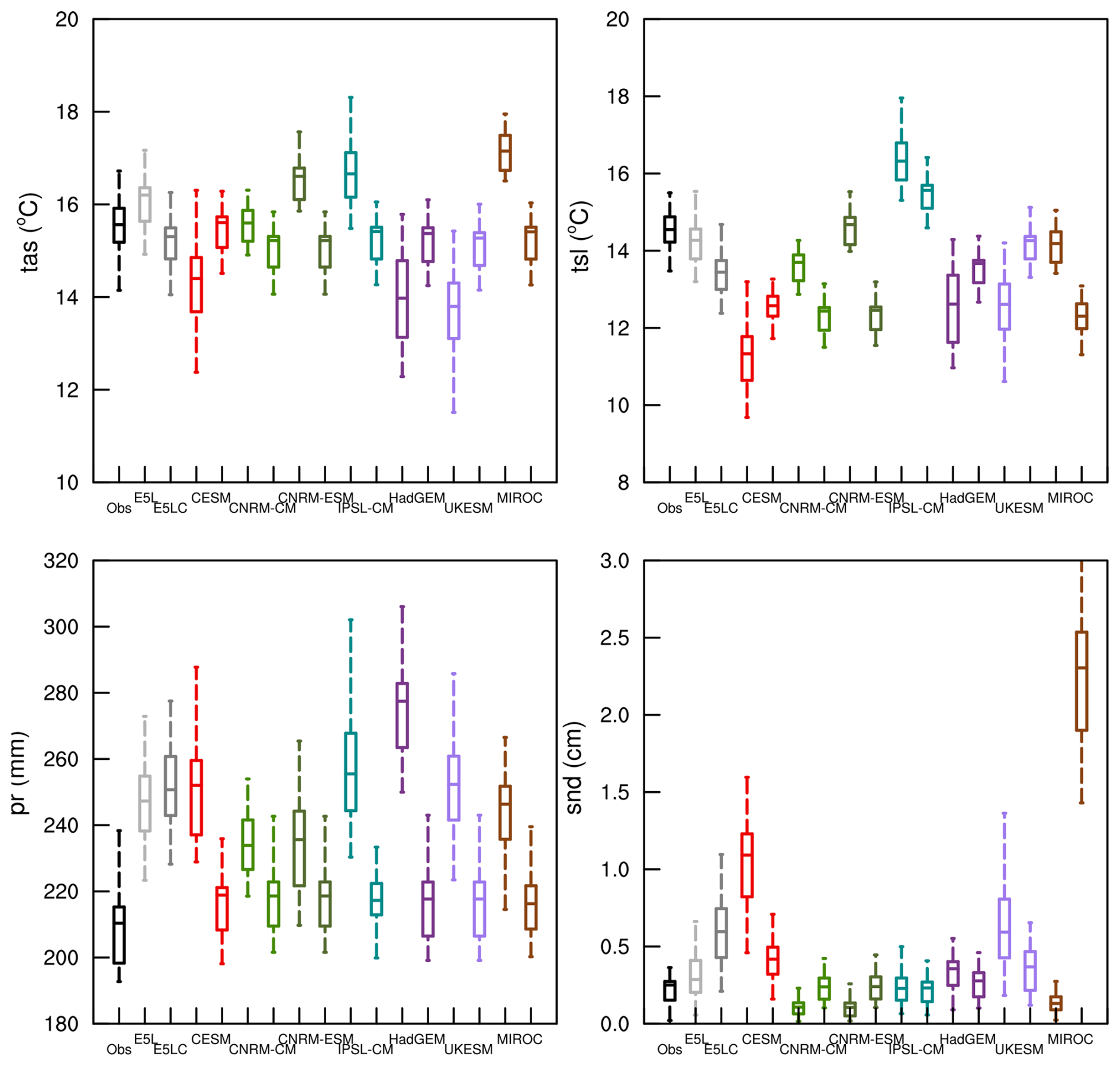
Figure A1 Sites' locations averaged JJA-climates (1985–2014) of hydrothermal variables as observed and simulated. Names on the x-axis and the colors indicate the different data sources. Model names indicate CMIP6 model output (left), and LS3MIP (right; see Table 1). Each CMIP6-LS3MIP pair shares the same color. The boxes represent the medians, first and third quartiles; the ± 1.5 × IQR or the maximum and minimum values, if within the former range, are taken as the whiskers' length.

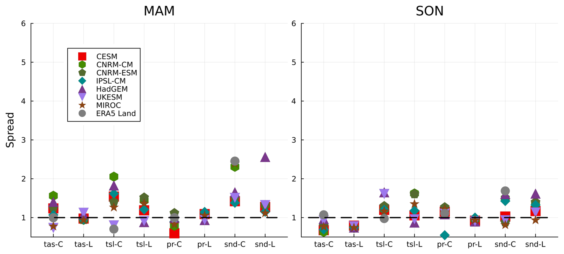
Figure A2 Relative spread (RS) of the sites-averaged climates (1985–2014) of the four variables in both ensembles and in E5LC with reference observations for all seasons. The colors indicate the models, and the x-axes show the variables and ensembles (C indicates CMIP6, and L indicates LS3MIP runs).

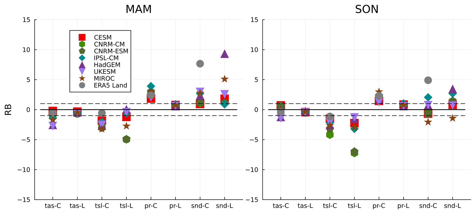
Figure A3 Same as in Fig. A2, but for relative biases (RB). The dashed lines (from −1 to 1) indicate the range of absolute median differences smaller than the observation's IQR.

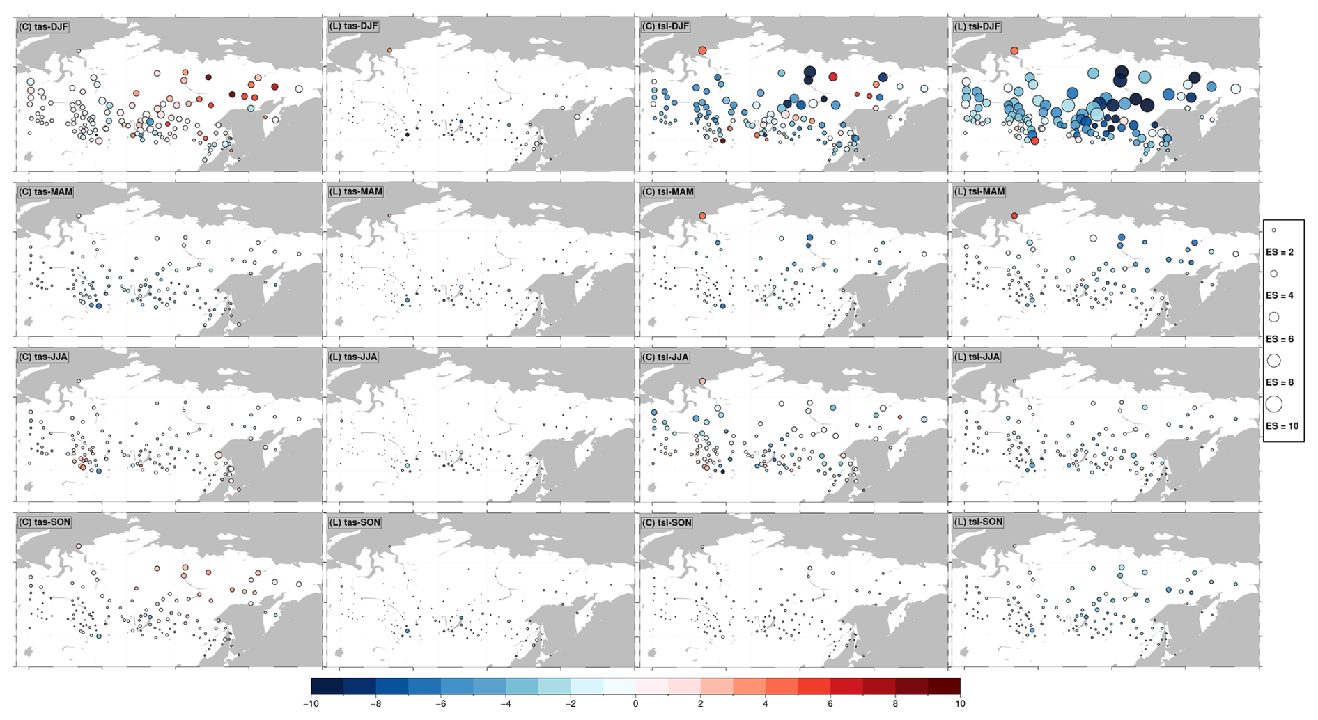
Figure A4 Weighted multi-model mean biases (EB) and their standard deviations (ES) of tas and tsl at observational sites in °C. The first and third columns are the results of CMIP6 models, and the second and fourth columns are the results of LS3MIP models. The first to fourth rows show the DJF, MAM, JJA, and SON seasons, respectively. Colors indicate the bias value, while the circle radii represent biases' standard deviations, i.e., the ensemble spread.

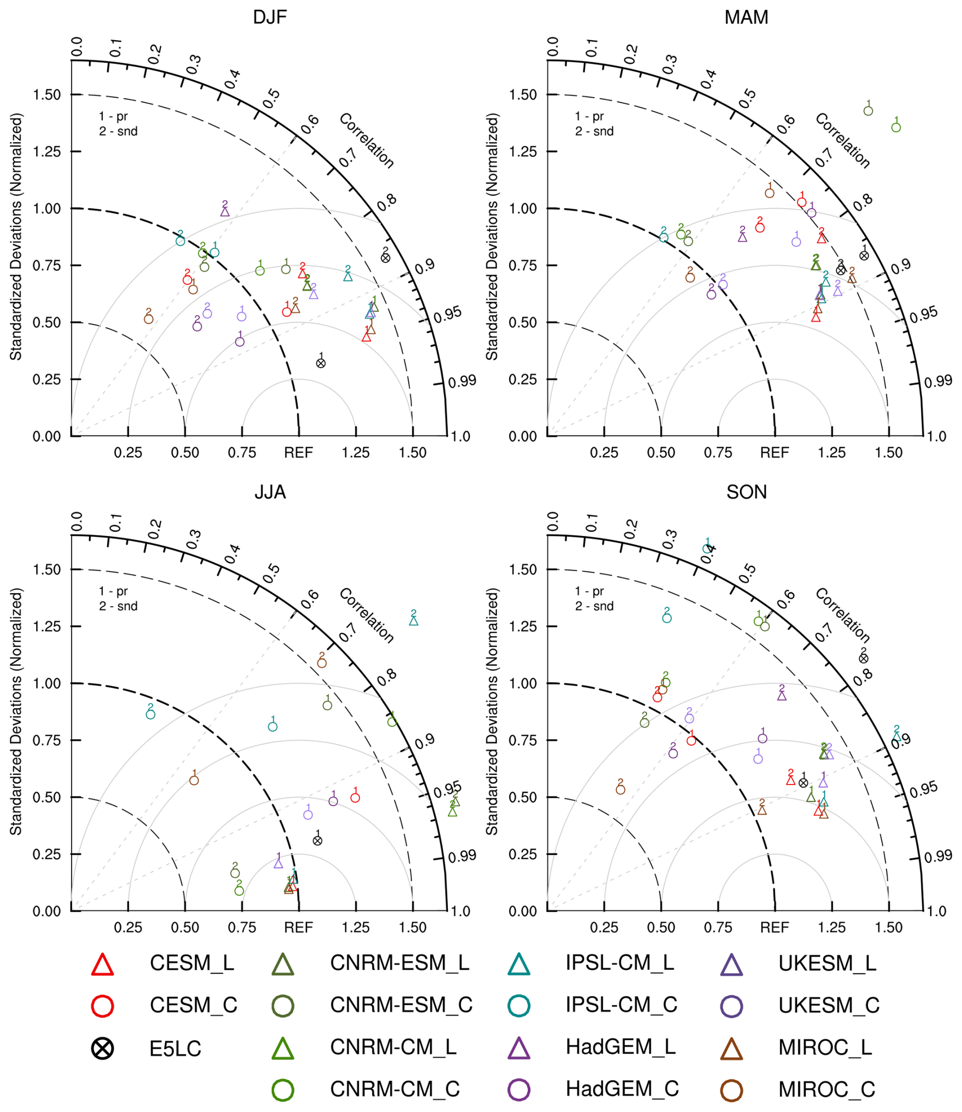
Figure A5 Taylor diagrams indicating the spatial correlation, standard deviation, and unbiased root-mean-square (RMS) difference (gray circles) for the four seasons of the simulated variables pr, snd (labeled by numbers) against observations at valid permafrost sites (here: sites with mean winter tas < −25 °C). Normalization is applied using the standard deviations of the observations. Colors indicate different models, and black crossed circles indicate E5LC. Triangles show the results of the LS3MIP runs, and solid circles of the CMIP6 runs.

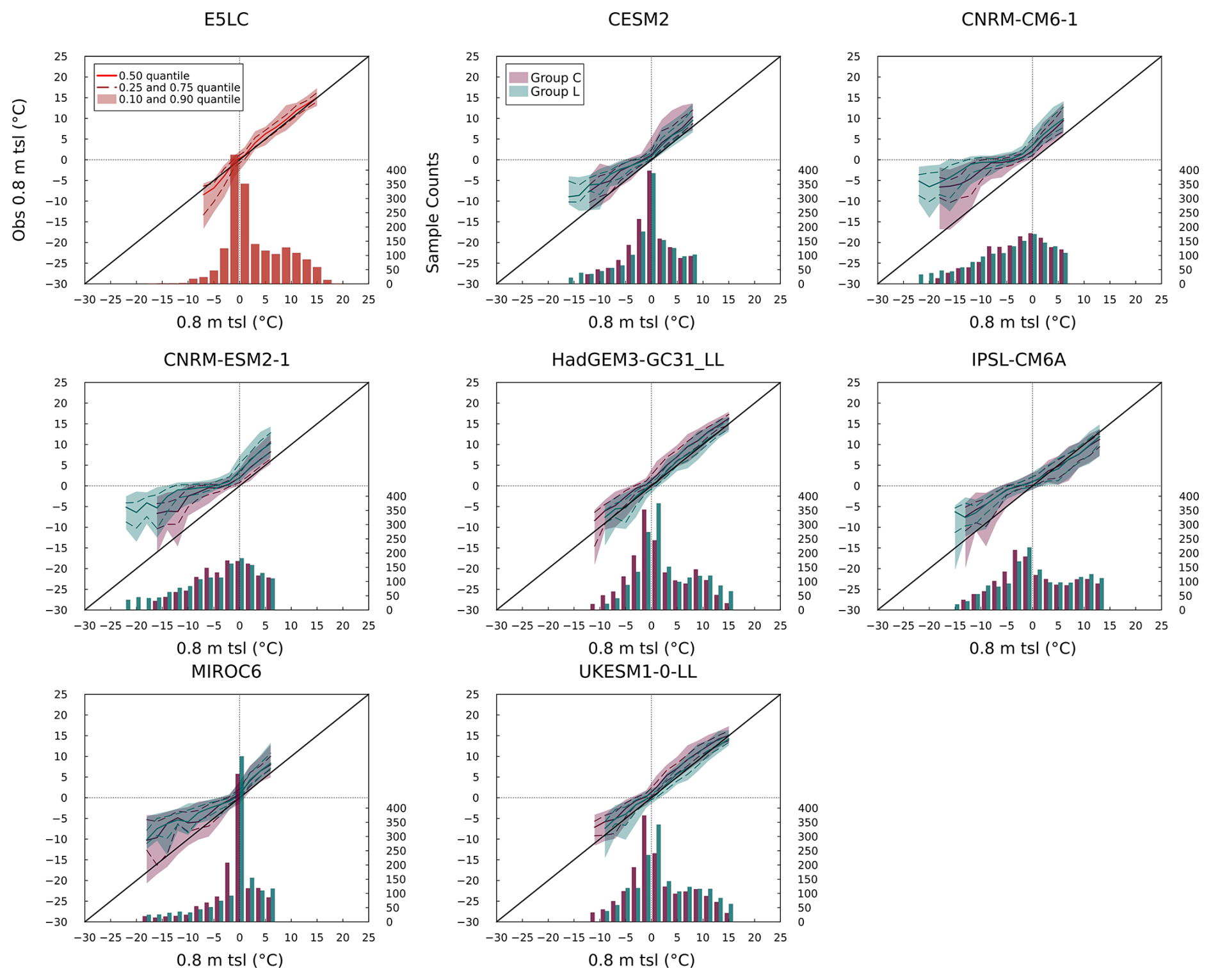
Figure A6 Quantile-Quantile (Q-Q) and histogram plots for soil temperature in depth 0.8 m. The plots show 30 year mean monthly 0.8 m tsl data of models at all sites and their observational values. The model simulations are binned into 2 °C intervals. Each bar (or pair of bars for CMIP6 and LS3MIP) is plotted at the center of its interval (e.g., 1 °C for 0 to 2 °C). The solid and dashed colored curves represent the median and $\mathrm{1}\mathrm{st}/\mathrm{3}\mathrm{rd}$ quartiles, respectively, of the corresponding observations for all data points within the temperature interval. The shaded area indicates the interdecile range. The histograms represent the sample size within each temperature interval, and temperature intervals with sample sizes smaller than 20 are excluded from the Q-Q plots. The further away the data is from the diagonal line, the larger the model's simulation bias is at certain temperature states. A higher vertical quantile range indicates more inconsistency with observation under identical temperature conditions.

Figure A7 Same method as Fig. A6, but for soil temperature at a depth of 1.6 m.

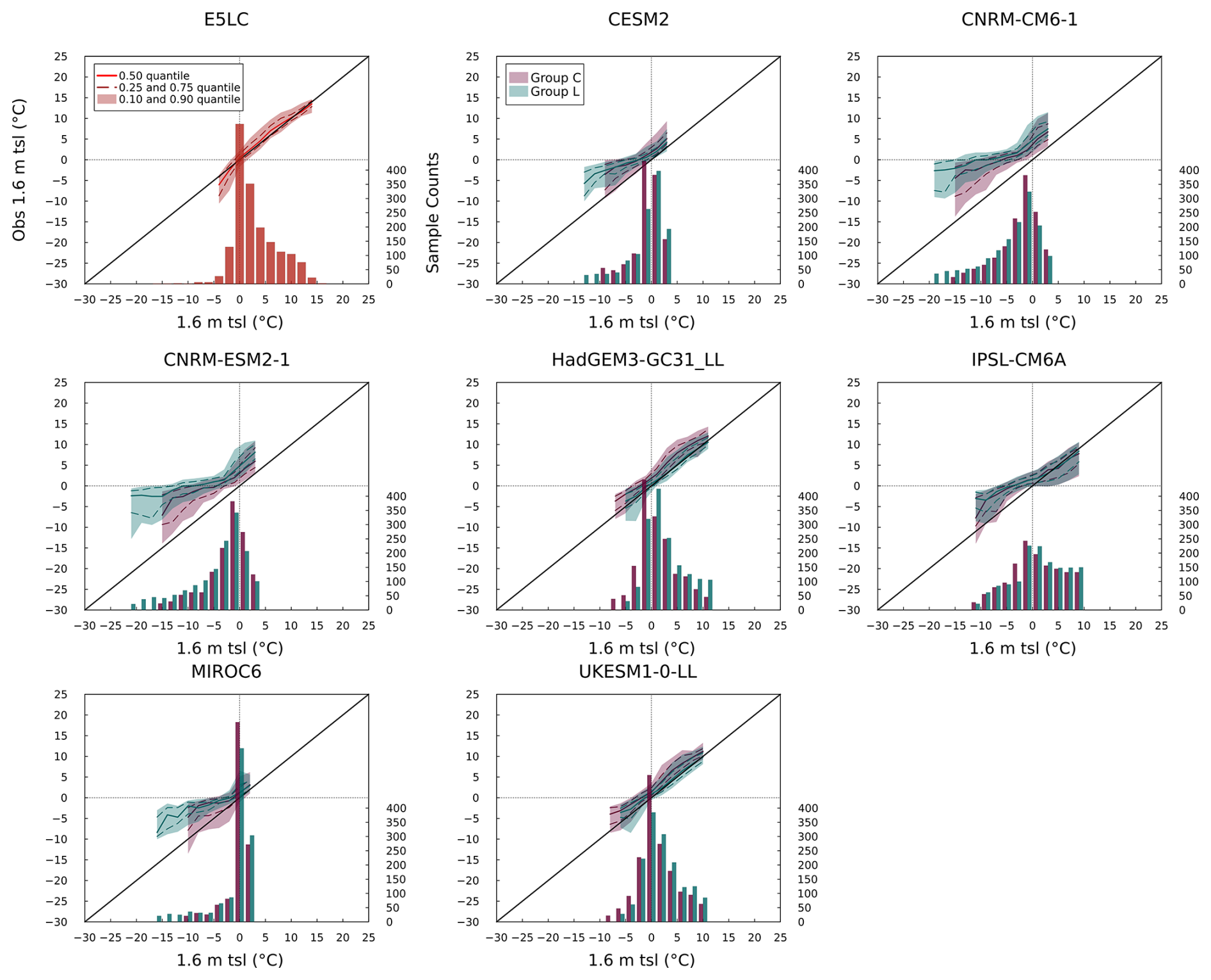
Table A1 Root-mean-square error (RMSE) between modeled and observed snow insulation effect (relationship between snow depth and soil–air temperature differences) across three tas categories, within the 0–0.8 m snow depth range (excluding fill-values) in °C, as illustrated in Fig. 10. The three lowest RMSE values in each column are indicated by bold font.