Lessons for multi-model ensemble design drawn from emulator experiments: application to a large ensemble for 2100 sea level contributions of the Greenland ice sheet

Multi-model ensembles (MME) are key ingredients for future climate projections and the quantification of their uncertainties. Developing robust protocols to design balanced and complete computer experiments for MME is a matter of active research. In this study, we take advantage of a large-size MME produced for Greenland ice sheet contributions to future sea level by 2100 to define a series of computer experiments that are closely related to practical MME design decisions: what is the added value of including a specific set of members in the projections, i.e. either adding new models (Regional Climate Model, RCM, or Ice Sheet Model, ISM) or extending the range of some parameter values? We use these experiments to build a random-forest-based emulator, whose predictive capability to assess Greenland sea level rise contributions in 2100 proves very satisfactory for low and high levels of warming but less effective for intermediate levels. On this basis, we assess the changes in the emulator's predictive performance, both in terms of prediction accuracy and uncertainty, and the emulator-based probabilistic predictions, in terms of changes in the 17th, 50th and 83rd percentiles, for given temperature scenarios, compared to the reference solution built using all members. For the considered MME, several aspects are outlined: (1) the highest impact of removing the most selected RCM, i.e., MAR, due to the large number of simulations available; (2) the significant impact of excluding the SSP5-8.5 scenario for high temperature scenarios, and of the Community Ice Sheet Model (CISM) for low temperature scenarios leading to absolute changes up to 30 % of the high and low percentiles respectively; (3) the non-negligible impact of having a MME designed with a unique ISM or a unique RCM, i.e., CISM or MAR model in our case, leading to percentile absolute changes ranging between 10 % and 20 % compared to the reference solution; (4) the lesser importance of the choice in the range of the Greenland tidewater glacier retreat parameter. These results point to the size of the training set as the key driver of the changes, which supports the need for large ensembles to develop accurate and reliable emulators, hence encouraging large participation to projects such as the Ice Sheet Model Intercomparison Project ISMIP. We also expect our recommendations to be informative for the design of next generations of MME, in particular for the next Ice Sheet Model Intercomparison Project in preparation (ISMIP7).

1 Introduction

Multi-model ensembles (MME) are key ingredients for future climate projections and the quantification of their uncertainties. They consist of sets of numerical experiments performed under common forcing conditions with different model designs (i.e. different model formulations, input parameter values, initial conditions, etc.) to generate multiple realisations known as ensemble members. This is the approach of Model Intercomparison Projects, MIPs, which are key for the understanding of past, present, and future climates and contribute to assessments from the Intergovernmental Panel on Climate Change (IPCC; e.g., Lee et al., 2021). In this study, we are interested in projected Greenland ice sheet contributions to sea level change this century, which are the subject of recent MME studies (Goelzer et al., 2018, 2020) within the Ice Sheet Model Intercomparison Project for CMIP6 (ISMIP6: Nowicki et al., 2016, 2020).

However, interpreting MME results is complicated by the choices made in their construction (e.g., Knutti et al., 2010). Ideally, the MME should evenly span a representative and exhaustive set of plausible realisations of the combined sources of uncertainty, e.g. distinct climate models with different but plausible strategies for simulating the global climate (GCMs), equally represented by a single model run. However, members of a MME are often structurally similar, and the degree of their dependence is difficult to quantify (e.g., Merrifield et al., 2020). This difficulty is particularly emblematic of the Coupled Model Intercomparison Project (CMIP), coined an “ensemble of opportunity” (Tebaldi and Knutti, 2007) because it collects “best guesses” (Merrifield et al., 2020) from modelling groups with the capacity to participate. This capacity may range from substantial resources to develop climate models and perform relatively large ensembles through to the ability to perform only a small number of simulations with an existing version of a climate model. These disparities, combined with the high computational expense of climate models and the partial dependence of MME members, results in limited and unbalanced multi-model ensemble designs, in which various combinations of modelling choices and forcing conditions are either over-represented or missing in the MME, and a full sampling of modelling uncertainties is impossible to perform or even to define. Section 2.1 provides in the following an illustration for the MME considered in this study.

Emulators (also named surrogate models) have been proposed to address these limitations. An emulator is a fast statistical approximation of a computationally expensive numerical model, often building on machine learning techniques like linear-regression (Levermann et al., 2020), Gaussian process regression (Edwards et al., 2021), random forest regression (Rohmer et al., 2022), and deep learning-based methods (Van Katwyk et al., 2025). Their key advantage is that they can be used to predict with low computational cost the numerical model's response at untried input values, and to explore the uncertain input space far more thoroughly. They can therefore potentially overcome the incompleteness of ensemble designs, which is essential for producing reliable probabilistic projections.

Some emulation studies have broadened this approach to represent entire MME at once, rather than individual models. One example in this field is provided by Edwards et al. (2021), who emulate ISMIP6 simulations for the Greenland and Antarctic ice sheets and multi-model glacier ensembles, driven by multi-model climate model ensemble simulations, to estimate land ice contributions to twenty-first-century sea level rise. Emulating an MME requires an assumption (and check) that the simulations are quasi-independent, i.e., that the differences induced by different model setups (in particular, initialisation) outweigh any similarities induced by common model structures. This was found by Edwards et al. (2021) to be the case for ice sheet and glacier MMEs. Another example is the study by Seroussi et al. (2023), who used a statistical emulator to recreate some of the missing simulations as done by Edwards et al. (2021) in order to investigate the dynamic vulnerability of major Antarctic glaciers using the ISMIP6 ensemble of ice flow simulations. Finally, another type of application is illustrated by Van Breedam et al. (2021) who used emulators to perform a large number of sensitivity tests with numerical simulations of ice sheet–climate interactions on a multi-million-year timescale.

In this study, we aim to explore how the results provided by an emulator can be informative for the design of an MME. Key design questions relate to the added value of including specific sets of experiments in the projections, i.e. either adding new models (e.g. new Regional Climate Model, RCM, new GCM, etc.) or extending the range of some parameter values (e.g., the Antarctic basal melt parameter or Greenland tidewater glacier retreat parameter described by Edwards et al., 2021). To address these questions, we take advantage of a large MME of Greenland ice sheet contributions to sea level this century, based on which we define a series of numerical experiments (referred to as emulator's experiments) that are closely related to practical MME design decisions. These experiments consist in leaving out specific results from the original MME assuming that all members have the same weight in the ensemble. The evaluation of the emulator prediction capability as well as the changes in probabilistic predictions induced by each of these emulator experiments provides us with information on the added value of including specific set of members and the impact of excluding groups of members.

The paper is organized as follows. We first describe the sea level numerical simulations as well as details of the statistical methods used to build the emulator and assess the different design questions (Sect. 2). In Sect. 3, we apply the experiments and assess the influence of each design question. We discuss results in Sect. 4, and we draw lessons and guidance related to the MME design, and discuss the implications from a stakeholder's point of view. Finally, we conclude in Sect. 5.

2 Data and methods

2.1 Multi-model ensemble case study

We focus on the sea level contribution, denoted slc (expressed in meters sea level equivalent, SLE, with respect to 2014), from the Greenland ice sheet (GrIS). Our study is based on a new MME study performed for the European Union's Horizon 2020 project PROTECT (http://protect-slr.eu, last access: 28 November 2025). Some modelling choices are taken from the protocols of the ISMIP6 initiative (Goelzer et al., 2020; in particular, the two main emissions scenarios, and the retreat parametrisation described below). This MME has been designed as an extension of ISMIP6 MME through the inclusion of:

• a wider range of CMIP6 climate model output as well as more climate change scenarios {SSP1-2.6, SSP2-4.5, SSP5-8.5};

• the surface mass balance forcing from several RCMs, i.e., MAR, RACMO, and HIRHAM as well as a statistical downscaling approach of a given GCM;

• retreat forcing before 2015 that is calculated from reconstructions of past runoff and ocean thermal forcing (Slater et al., 2019, 2020), hence allowing for a consistent forcing of the models in past and future (Rahlves et al., 2025) and to consider historical retreat of the outlet glaciers, which was an important source of mass loss after 1990.

We provide here a brief summary of the GrIS MME dataset and refer the interested reader to Goelzer et al. (2025) for further details, where appropriate. The full modelling chain for these projections combines: (1) a number of CMIP5 and CMIP6 GCMs that produce climate projections according to different emissions scenarios; (2) different RCMs, and their variants, that locally downscale the GCM forcing to the GrIS surface; (3) a range of ISM models that produce projections of ice mass changes and slc (initialised to reproduce the present-day state of the GrIS as best as possible, at a given initial year sometime before the start of emissions scenarios in 2015). The ISMs are forced by surface mass balance (SMB) anomalies from the RCMs, added to their own reference SMB assumed during initialisation. Ocean forcing is integrated based on an empirically derived retreat parameterization that relates changes in meltwater runoff from the RCM and ocean temperature changes from the GCM to the retreat of calving front positions (Slater et al., 2019, 2020). The parameter that controls retreat is denoted κ. It represents the sensitivity of the ocean forcing as a whole, and defines the sensitivity of the downscaling from global model to local ice sheet scale. Figure 1 shows the general approach used for forcing the ISMs and producing the projections. The MME design questions addressed in this study are related to the modelling choices made for each of the boxes outlined in Fig. 1.

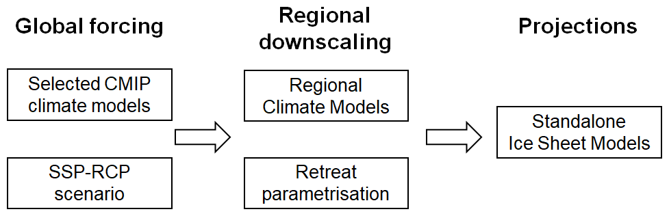
Figure 1 General forcing approach for Greenland ice sheet model projections. The questions relevant for the MME design (detailed in Table 2) are related to the modelling choices made for each of the boxes.

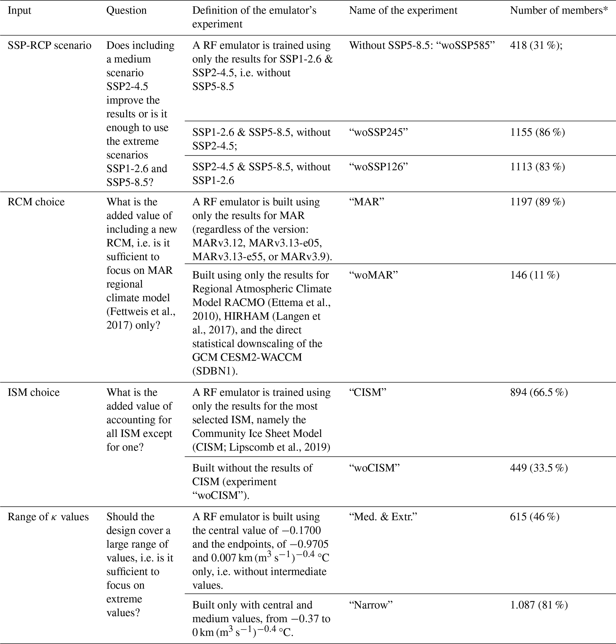
In what follows, we use the generic term “inputs” to designate all the choices made throughout the modelling chain, i.e. the choices in the models used, the choices in the scenarios and the ice-sheet parameter values. The inputs are described in detail in Table 1. All abbreviations used in the text are explained in Appendix E. The inputs below the double line in Table 1 are those used for the building of the RF emulator, in particular with the use of global annual mean surface air temperature change relative to 1995–2014, denoted GSAT, that corresponds to a combination of SSP-RCP and GCM by following a similar approach as Edwards et al. (2021).

Table 1 Inputs considered in the GrIS MME. The inputs below the double line are those used for the building of the RF emulator described in Sect. 2.2.

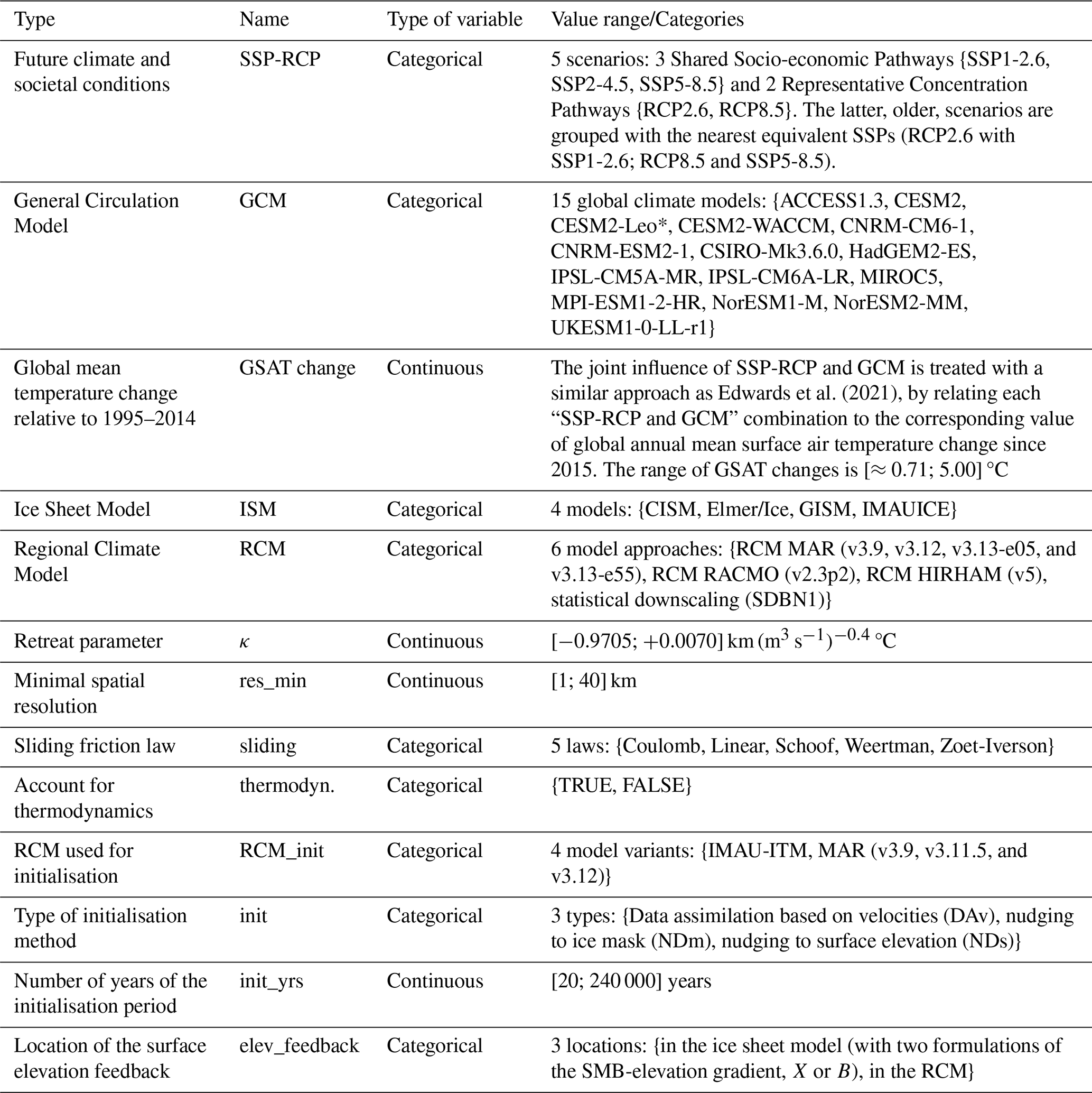
* CESM2-Leo is a variant pre-dating the official CESM2 release for CMIP6. It can be considered as another ensemble member of CESM2.

One input setting, i.e., a particular combination of inputs, defines a member of the MME. Formally, the inputs are either treated as continuous variables (e.g., for κ, minimum resolution), or as categorical variables (e.g., RCM or ISM choice). Figures 2 and 3 show the histograms for a selection of the continuous and categorical variables described in Table 1. For sake of space, we focus here on the 7 of 11 variables identified as having the largest influence on slc in 2100 (see Sect. 3 and Appendix C). Both Figs. 2 and 3 show that the design of experiments is unbalanced: some categories (like CISM model for instance for ISM in Fig. 2, top, left) or some values (like minimum resolution at 16 km, Fig. 3, centre) are more frequent than others. The design is also incomplete with large gaps in the continuous class. This is for instance the case for κ between −0.9705 and −0.3700 km (m³ s${}^{-\mathrm{1}}{)}^{-\mathrm{0.4}}$ °C (Fig. 2, left), because this parameter was sampled for only 3 different values by most models (the median, the 25 % and the 75 % percentile), and the additional 2 values were only sampled by one ISM at a later stage to broaden the parameter range.

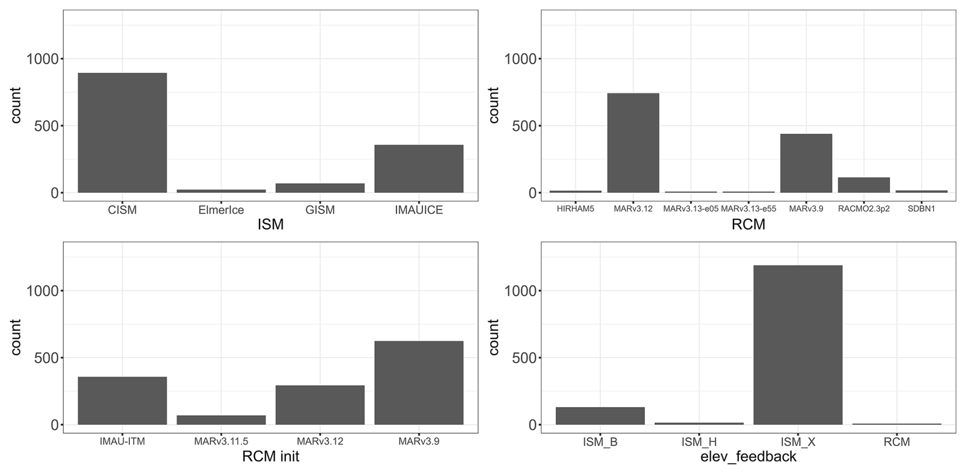
Figure 2 Count number of the MME members with respect to the different inputs classified as “categorical” in Table 1: ISM (ice sheet model), RCM (regional climate model used for downscaling climate projections), RCM init (regional climate model used for initialisation climate), and elev_feedback (approach to representing the feedback between the ice sheet surface elevation and climate).

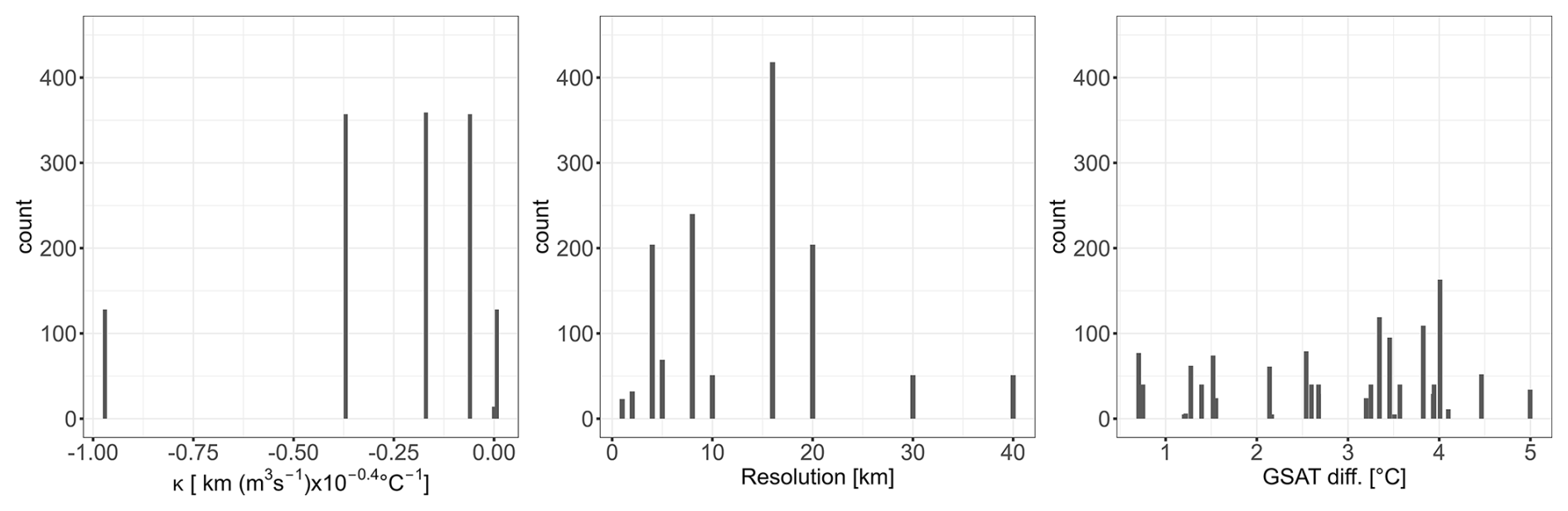
Figure 3 Count number of the MME members with respect to the different inputs classified as “continuous” in Table 1: κ (ice sheet tidewater glacier retreat parameter), minimum spatial resolution of the ice sheet model, and GSAT diff (global mean surface air temperature change relative to 1995–2014 during the driving global climate model simulation).

The considered MME comprises n=1343 members, which are used to estimate slc in 2100. In this study, we assume that each member has the same weight, in particular, without differentiating members based on their reliability (e.g., low-resolution models compared with high-resolution models) or any observational constraints (as done for instance by Aschwanden and Brinkerhoff, 2022). Under this assumption of uniform weighting, Fig. 4 shows a probability density distribution of slc constructed directly using the members of the MME, which has a median value of 8.7 cm SLE and 17 % and 83 % quantiles of 4.1 and 14.0 cm; the latter being used to define the 66 % confidence interval named “likely” following the IPCC terminology (Mastrandrea et al., 2010).

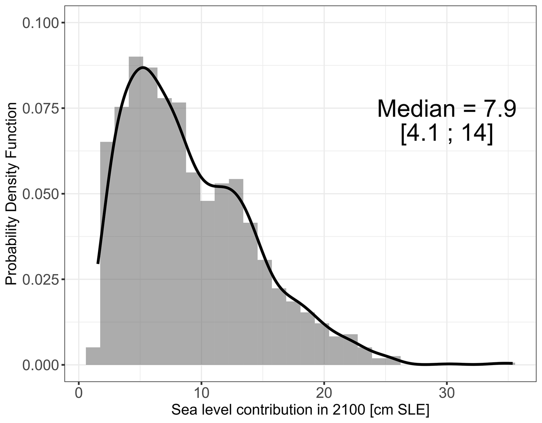
Figure 4 Probability density function of the sea level contribution of the Greenland ice-sheet in 2100, with respect to 2014, based on the raw MME ensemble data considered in this study assuming that each member has the same weight. The black straight line provides the smoothed density function. The median value and the likely range (66 % confidence interval) are also indicated.

Table 2 Design questions and corresponding emulator's experiments. Modelling choices are evaluated based on the RF emulator performance and the probability estimate of slc in 2100 given GSAT change relative to 1995–2014 at 2, or 4 °C (±0.5 °C).

* % of the total number of members

2.2 Emulator experiments related to design questions

In this study, we address a series of questions described in Table 2 that are relevant for the design of MMEs. In general, the central concern is to investigate what is the added value of including a specific set of experiments in the projections. This could be subsets in already defined value range/categories, or subsets not currently categorised. For four different categories of inputs related to specific modelling choices (choice in SSP-RCP, choice in RCM, choice in ISM, and range of κ values), the design questions are formalised in Table 2. To assess the added value of including a specific set of experiments in the projections, we propose to construct emulators by leaving out specific results from the original MME without differentiating the members, i.e., by assuming that all members have the same weight in the ensemble. The last column of Table 2 translates the design questions into a specific emulator's experiment. The modelling details are provided in Sect. 2.3.

To measure the influence of removing specific members from the original MME, we assess if the emulators constructed from the reduced MME can reproduce the results of an emulator trained with the complete original MME, named the “reference solution” in the following. We analyse the changes in two types of criteria: (1) emulator performance to predict slc in 2100 for input configurations unseen during the training; (2) probabilistic predictions for slc in 2100 given future GSAT change scenarios, here chosen at 2 °C (±0.5 °C) or 4 °C (±0.5 °C) relative to 1995–2014. The details of this assessment are explained in Sect. 2.4. Quantified criterion changes are then used to rank the different emulator experiments in terms of the magnitude of their impact on emulator performance and emulator-based probabilistic predictions.

2.3 Prediction with random forest emulators

The objective is to predict slc in 2100 from any values (configurations) of the different inputs (described in Table 1). We replace the chain of numerical models described in Sect. 2.1 by a machine-learning-based proxy (named emulator) built using the MME results. Among the different types of emulators (see a recent overview by Yoo et al., 2025), we focus in this study on the Random Forest (RF) regression model, as introduced by Breiman (2001). RF has shown high efficiency in diverse domains of application (sea level science, Tadesse et al., 2020; water resources, Tyralis et al., 2019; flood assessments, Rohmer et al., 2018), and more particularly for sea level projection studies (Hough and Wong, 2022; Rohmer et al., 2022; Turner et al., 2024).

The RF regression model is a non-parametric technique based on a combination (ensemble) of tree predictors (using regression tree, Breiman et al., 1984). By construction, tree models are well adapted to deal with mixed types of variables, categorical or continuous, as is the case here (see Table 1). Each tree in the ensemble (named forest) is built based on the principle of recursive partitioning, which aims at finding an optimal partition of the input parameters' space by dividing it into disjoint subsets to have homogeneous slc values in each set by minimizing the variance splitting criterion (Breiman et al., 1984). A more complete technical description is provided in Appendix A.

A key aspect of our study is to be able to handle many categorical variables with large number of levels (unordered values). However, the partitioning algorithm described above tends to favour categorical predictors with many levels (Hastie et al. (2009): Chap. 9.2.4). To alleviate this problem, we rely on the computationally efficient algorithm proposed by Wright and König (2019) based on ordering the levels a priori, here by their slc mean response.

A second key aspect is to be able to predict for new levels of the categorical variables, since the emulator experiments defined in Sect. 2.1 involve leaving out specific members from the original MME assigned to a given model, RCM/ISM, or a given SSP-RCP scenario, i.e., some specific levels. This problem is related to the more general “absent levels” problem for RF models (Au, 2018), which arises when a level of a categorical variable is absent when a tree is grown, but is present in a new observation for prediction. Here, the chosen ordering algorithm of Wright and König (2019) alleviates this problem: by treating the categorical variables as ordinal, levels not present at a given partition during the splitting procedure can still be assigned to a next partition in the next iteration by directing all observations with absent levels down the same branch of the tree (in our implementation, chosen as the “left” branch). In this manner, the observations with absent levels are kept together and can be split down the tree by another input variable. In our study, this means that the emulator experiments test whether the information left in the MME after removing specific members is sufficient to predict slc at a reasonable accuracy.

Finally, it is important to note that the emulator is a statistical approximation whatever the regression method used, i.e. it uses only a limited number of numerical results, i.e. inputs-slc pairs (corresponding to the training data), to perform predictions given a “yet-unseen” inputs' configuration. Such an approximation introduces a new source of uncertainty referred to as “emulator uncertainty” as discussed by Storlie et al. (2009). To assess this type of uncertainty, we rely on the RF variant specifically developed by Meinshausen (2006) for predicting quantiles, i.e. the quantile RF model (qRF) as described in Appendix B. The advantage is that prediction intervals can be calculated at any level, which can be used to reflect the uncertainty of the RF emulator in emulator predictions.

In summary, the emulator provides a “best estimate”, corresponding to the mean provided by the RF model (Appendix A), and prediction intervals at level α, denoted PI^α, constructed from the conditional quantiles of the qRF model (Appendix B). In what follows, we indifferently designate the emulator used as the “RF model”.

2.4 Criteria for measuring the impact of the design questions

2.4.1 Emulator performance

The first criterion measures the decrease in the predictive performance of the emulator. It is assessed through a validation test exercise that consists in repeating 25 times the following procedure:

1. Split the original MME into a test set T composed of n_test randomly selected test samples and a training set MME_tr;

2. Apply the emulator experiments “exp” described in Table 2 by removing specific members from MME_tr. The resulting reduced set ${\mathrm{MME}}_{\mathrm{tr}}^{\exp }$ is used for the training of the emulator RF^exp;

3. The trained models RF^exp are used in turn to predict slc for the prediction samples of T;

4. Train an emulator RF^ref with all samples of MME_tr. This emulator is used to estimate the reference solution using T.

In this study, we are more particularly interested in the ability of the emulator to perform well over a wide range of GSAT change values. This is important in our case, because constraining the predictions to temperature constraints can help end-users to interpret the projections as illustrated by recent projections for France by Le Cozannet et al. (2025), although it should be noted that our definition of GSAT change does not correspond to the usual definition of global warming level (GWL) as being relative to the preindustrial.

We propose a procedure for selecting the test samples at step (1) of the validation procedure as follows: (i) the GSAT changes are classified into a finite number of intervals, the ends of which are defined by the GSAT change percentiles, with levels ranging from 0 % to 100 % with a fixed increase of 25 %. This results in the following GSAT change intervals, [0.705; 2.14 °C], [2.14; 3.34 °C], [3.34; 3.83 °C], and [3.83; 5.00 °C]; (ii) for each interval, 50 samples are randomly selected. Consequently, for one iteration of the validation procedure, a total of n_test=200 test samples are randomly selected. By doing so, we ensure that the RF model is tested at each of the 25 iterations on samples that cover the full range of GSAT change values, with a fixed number of samples in each interval. This would not necessarily be the case when using the standard cross validation procedure (Hastie et al., 2009), where the test samples would be randomly selected regardless of their GSAT change value.

Five performance criteria (formally described in Appendix D) are considered:

• the mean relative absolute error, RAE, which measures the RF predictive capability, i.e. whether the RF emulator can predict slc with high accuracy given yet-unseen instances of the inputs. High predictive capability is achieved for a RAE value close to zero;

• the coefficient of determination, Q², which also measures the RF predictive capability by quantifying the amount of variance explained by the RF model. A high predictive capability is achieved for a Q² value close to one. A negative Q² means that the emulator performs worse than simply predicting the mean as a constant output prediction;

• the continuous ranked probability score, denoted CRPS, as used for validating probabilistic weather forecast (Gneiting et al., 2005), that jointly quantifies the calibration of qRF probability distribution, i.e. the reliability of the estimation, and its sharpness (i.e. the concentration/dispersion of the probability distribution). The lower CRPS, the higher the quality of the qRF probabilistic predictions, with a lower limit of zero;

• the coverage αCA¹⁻ of the RF prediction intervals PI^α at significance level α, which measures the proportion of slc values of the test set that falls within the bounds of the intervals. If αCA¹⁻ is close to the theoretical value of 1−α, this means that the prediction interval is statistically well calibrated, and its reliability can be considered satisfactory;

• the ratio of performance to the interquartile distance IQR (Bellon-Maurel et al., 2010), which compares the emulator prediction uncertainty, measured by the difference between the 75th and the 25th quantiles – named interquartile distance, with the prediction error measured by the root mean square error. If IQR ≈1, the interquartile distance provides valuable information about the prediction error. If IQR <1 (>1), this means that the emulator prediction uncertainty under-(over-)estimates the prediction error, i.e., the emulator provides over-(under-)confident predictions.

2.4.2 Emulator-based probabilistic predictions

The second set of criteria measures the changes in the emulator-based probabilistic predictions, which are assessed through a Monte-Carlo random sampling procedure by considering two GSAT change scenarios of 2 and 4 °C. The procedure holds as follows:

1. Randomly and uniformly sample the GSAT change values within the range defined by the GSAT change scenario value ±0.5 °C;

2. Randomly sample the input variables by assuming a uniform discrete probability distribution for the categorical variables, and a uniform probability distribution for the continuous variables except for κ which is sampled as in Edwards et al. (2021) from the smoothed version of the empirical density function by Slater et al. (2019). A total of 10 000 random samples is considered;

3. Apply the emulator experiments by removing specific members from the original MME, and train the corresponding emulator RF^exp;

4. Use RF^exp to predict slc for each random sample and estimate the median, i.e., the 50th percentile (denoted Q50%) and the endpoints of the 66 % confidence interval, named “likely range” following the IPCC terminology, defined here by the 17th and 83rd percentile, denoted Q17% and Q83%.

To derive the reference solution of the quantiles of interest, the afore-described procedure is applied to the RF emulator trained with the original MME. In addition, the emulator uncertainty is propagated by following the procedure based on the quantile RF emulator (Appendix B). The emulator-based probabilistic results thus jointly reflect the impact of the uncertainty of the input variables and of the emulator uncertainty. The probabilistic predictions should however not be interpreted as calibrated uncertainty accounting for model-observation misfits (e.g., Aschwanden and Brinkerhoff, 2022), and neither do they represent the slc probability distribution from the MME, because the uniform distribution over the input space is not representative of the MME itself.

3 Results

3.1 Emulator reference solution

We train a RF emulator to predict slc in 2100 using the results of the GrIS MME (see implementation details in Appendix A). A preliminary screening analysis was conducted (detailed in Appendix C), and showed that four predictor variables have no significant influence: the choice to account for thermodynamics, the choice in sliding law, the type of initialisation and the number of years for the initialisation phase. We therefore build the RF emulator using only 7 out of 11 possible input variables described in Sect. 2.

Figure 5 Boxplot of the RAE (a), Q² (b), CRPS (c), CA⁹⁰ (d), CA⁵⁰ (e), and IQR (f) performance criterion for different ranges of GSAT change values (indicated on the x axis). The performance statistics are computed over test samples unseen during emulator training by applying the validation procedure described in Sect. 2.4.1 repeated 25 times. The horizontal red dashed line indicates the median value calculated over all validation tests considering the whole range of GSAT change.

Based on the full MME, we compute the reference solution for the criteria used to investigate the influence of the design questions. First, the RF model's predictive performance is tested by applying the repeated validation procedure described in Sect. 2.4.1. The performance of the RF emulator shows satisfactory levels of predictive capability, with a median RAE value (calculated over all the validation tests defined by the repeated validation procedure) of no more than 8 %, a median Q² value close to 90 % and a median CRPS value close to zero as indicated by the dashed red horizontal line in Fig. 5a–c. In addition, the RF emulator appears to be well calibrated both in terms of coverage of the prediction intervals at the 10 % (Fig. 5d) and the 50 % (Fig. 5e) significance level, and in terms of interquartile distance with a median IQR close to 100 % (Fig. 5f).

The examination of the performance depending on the GSAT change interval of the test samples (coloured boxplots in Fig. 5) further shows that the highest performance is achieved for low GSAT change below 2.14 °C (dark blue boxplots in Fig. 5) although we note a small overestimation of the coverage at 50 %, and a tendency for underconfident predictions with IQR >100 %. The worst performance is achieved for GSAT change between 3.34 and 3.83 °C (green boxplot in Fig. 5). The performance for the other GSAT change intervals, and in particular for the highest GSAT change values above 3.83 °C, can be considered satisfactory with a median RAE not larger than 9 %, a median Q² value close to 90 %. The prediction intervals are well calibrated with a median coverage CA⁹⁰ and CA⁵⁰ of 86 % and of 46 %, and with a small tendency for overconfident predictions with a median IQR of ≈82 %.

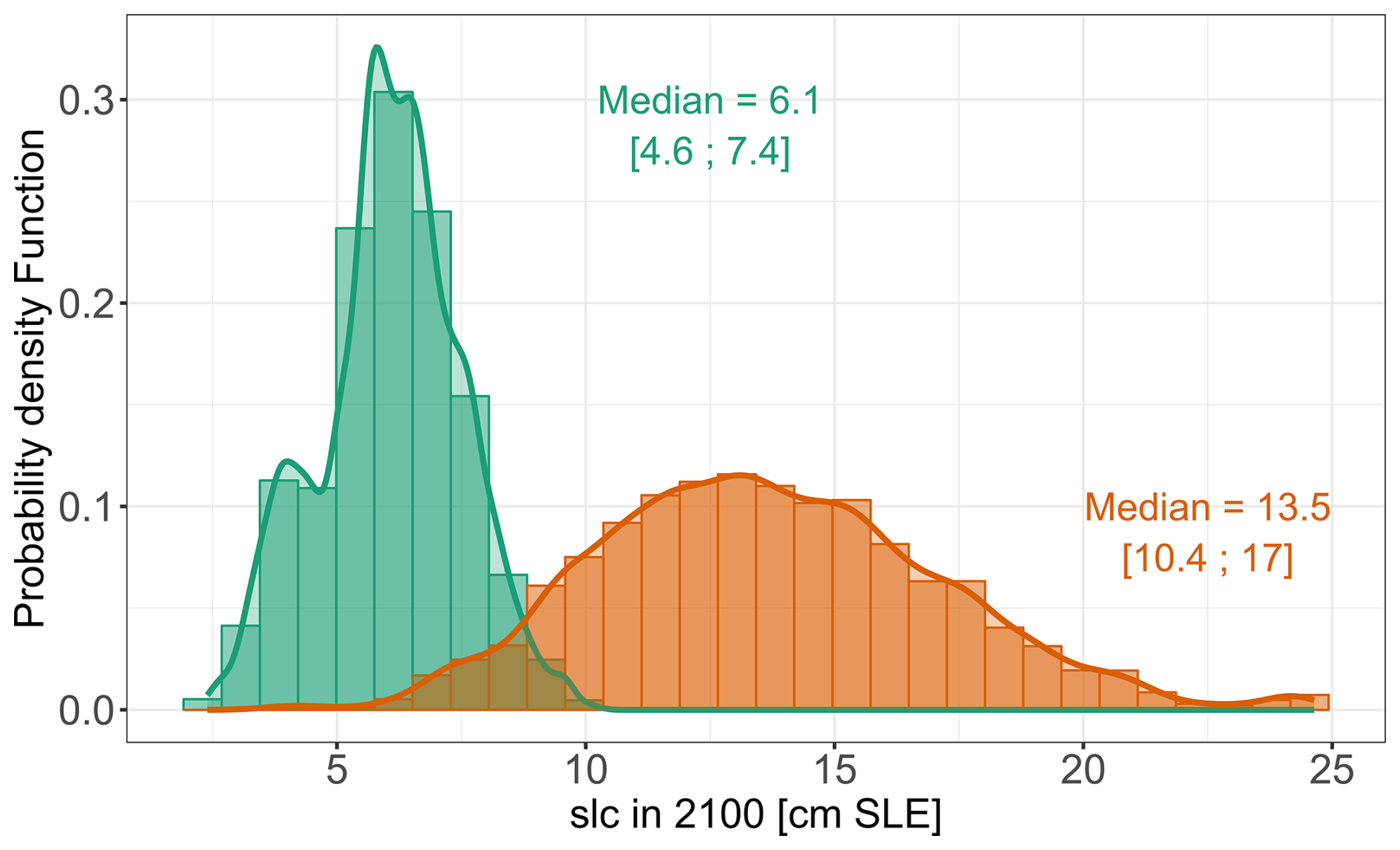
Figure 6 Emulator-based probabilistic predictions in the form of the probability density function of slc in 2100 (with respect to 2014) constructed using the Monte-Carlo-based procedure (with 10 000 random samples, see Sect. 2.4) for two GSAT change values of 2±0.5 °C (green), and 4±0.5 °C (orange) relative to 1995–2014. This results in a median value of respectively 6.7 and 13.5 cm with a likely range of [4.6; 7.4] cm, and [10.5; 17.0] cm. The straight line corresponds to the smoothed density function. The number and interval indicate the median value and the likely range. Note these probability density functions are derived using the mean of the RF emulator (Appendix A) and do not include uncertainty arising from the emulator itself.

Second, the probability distribution of slc in 2100 relative to 2014 (Fig. 6) is constructed using the Monte-Carlo-based procedure (with 10 000 random samples) described in Sect. 2.4.2 given GSAT change values fixed at 2 and 4 °C (±0.5 °C). The choice of GSAT change scenarios used here is supported by the afore-described analysis, which points out that the RF emulator should be used cautiously over the range of GSAT change values around 3 °C. The emulator-based probabilistic prediction results in a median value of respectively 6.1 and 13.5 cm for slc with a likely range of [4.6; 7.4] cm, and [10.4; 17.0] cm. The results are computed using the mean of the RF emulator (Appendix A), and do not include uncertainty arising from the emulator itself. The procedure described in Appendix B is further applied to assess the impact of the emulator uncertainty, and shows that the width of the 90 % confidence interval for the percentiles considered remains in the order of 0.1 cm, hence indicating minor influence of the emulator uncertainty in this case.

3.2 Impact of design decisions on the emulator performance

We analyse in Fig. 7 the impact of design decisions on the RF predictive capability and on the reliability of the RF prediction intervals. The decrease of RF predictive capability is measured by the decrease of the relative differences of RAE and CRPS (Fig. 7a, c) and the increase of the relative differences of Q² (Fig. 7b). The reliability of the RF prediction intervals is measured by CA⁹⁰ and CA⁵⁰ (Fig. 7d, e), which are respectively related to the prediction intervals at the 10 % and 50 % significance level, and by IQR (Fig. 7f). This assessment is conducted relative to the performance metrics of the reference solution computed from the validation test applied without excluding the experiments as explained in Sect. 2.4.1.

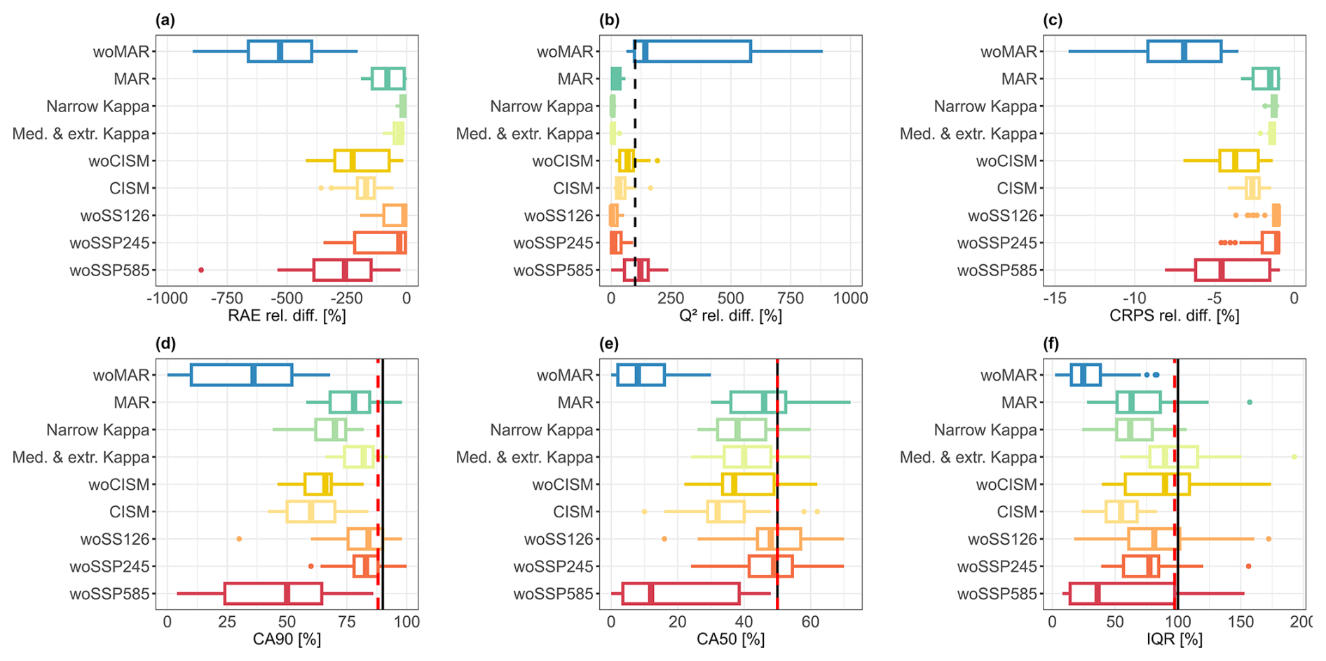
Figure 7 Relative difference (in %) of the performance criteria for RAE (a), Q² (b), CRPS (c). Evolution of CA⁹⁰ (d), CA⁵⁰, and IQR (f). The performance statistics are computed over test samples unseen during emulator training by applying the validation procedure described in Sect. 2.4.1 repeated 25 times. The dashed black line in panel (b) indicates the threshold under which the emulator performs worse than simply predicting the mean as a constant output prediction. The straight black line in panels (d)–(f) indicates the theoretical threshold that the emulator should reach. The red dashed line indicates the median value of the RF reference solution.

Figure 7 shows that excluding MAR (experiment “woMAR”) has the largest impact for every performance criterion. This is also shown when considering a given GSAT change interval in the validation procedure (Figs. 8 and 9 and Sect. S1). This means that excluding MAR impacts both facets of the predictive capability of the emulator, i.e., the explained variance of the emulator Q² and the relative errors RAE (Fig. 7a, b). In particular, the resulting relative difference is >100 %, i.e., Q²<0, hence showing that the emulator performs worse than simply predicting the mean as a constant output prediction. This performance decrease goes with a decrease of the reliability in the prediction intervals as shown by the increase in CRPS (Fig. 7c). This is confirmed by the coverage values which largely deviate from the expected values (outlined in black in Fig. 7d, e). In addition, overconfident predictions are clearly shown by the low value of IQR. The examination of the opposite situation, i.e., the “MAR” experiment, shows that training the RF model with only the members associated with this particular RCM cannot be considered satisfactory. This is highlighted by the non-negligible changes in performance, specifically in terms of increases in RAE and CRPS and decreases in IQR (dark green box plots in Fig. 7), although they are significantly smaller in magnitude than those in the “woMAR” experiment.

The second most important driver of the emulator performance is the exclusion of the extreme SSP scenario SSP5-8.5 (dark red boxplot in Fig. 7) which induces a performance reduction of around half that of “woMAR” for RAE and CRPS. As for “woMAR”, the Q² reduction is so high that the resulting performance is worse than that of simply taking the mean value for prediction. The reliability of the prediction intervals appears to be very poor as well with large deviations from the expected values. The third most important contributor of the emulator performance is the exclusion of CISM with RAE and CRPS median values close to that of “woSSP585”, but with higher performance in terms of explained variance as indicated by a lower Q² relative difference, and more reliable prediction intervals.

Figure 8 Relative difference (in %) of the performance criteria considering the lowest GSAT change values below 2.14 °C (top) and the highest GSAT change values above 3.83 °C (bottom) for RAE (a, d), Q² (b, e), and CRPS (c, f). The performance statistics are computed over the same test samples as in Fig. 7. The black line in panels (b) and (e) indicates the threshold under which the emulator performance is worse than predicting the mean as a constant output prediction.

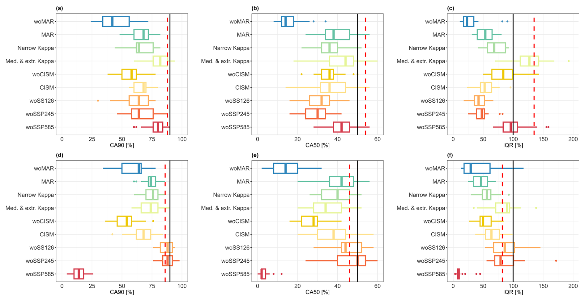
Figure 9 Evolution of the performance criteria considering the lowest GSAT change values below 2.14 °C (top) and the highest GSAT change values above 3.83 °C (bottom) for CA⁹⁰ (a, d), CA⁵⁰ (b, e), and IQR (c, f). The performance statistics are computed over the same test samples as in Fig. 7. The red dashed line indicates the median value of the RF reference solution. The black line indicates the threshold against which the performance criterion should be compared.

The ranking in terms of influence depends however on the range of GSAT changes considered. On the one hand, the following observations can be made for the highest GSAT change values:

• the application of experiments “woSSP585” and “woMAR” affects almost equivalently the emulator performance by inducing large changes in terms of RAE (Fig. 8d), Q² (Fig. 8e) and CRPS (Fig. 8f) relative differences. Here, the resulting predictive performance is worse than that of simply taking the mean value for prediction;

• the analysis of the prediction intervals (Fig. 9, bottom) shows that their reliability for “woSSP585” is worse than that of “woMAR” with very low coverage at any level (Fig. 9d, e) and extremely high overconfidence in the predictions (Fig. 9f);

• the influence of the “woCISM” experiment ranks third, with a decline in predictive capability on the same order of magnitude than that of “woSSP585” or “woMAR”, particularly in terms of RAE (Fig. 8d), but with higher reliability of the prediction intervals (Fig. 9, bottom);

• the analysis of “woSSP126” and “woSSP245” shows that the exclusion of these SSP scenarios has negligible impact for the highest GSAT change values.

On the other hand, the following observations can be made for the lowest GSAT change values:

• the experiment “woSSP585” is no longer the highest contributor to the predictive capability. The prediction intervals for “woSSP585” even reach coverage close to the expected value and the interquartile distance compares well with the prediction error;

• among the different SSP scenarios considered, it is the “woSSP245” scenario and, to a lesser extent, the “woSSP126” scenario, that causes the most significant reduction in performance for the lowest GSAT change scenario;

• the exclusion of CISM or of MAR drives here the most the performance with almost the same order of magnitude (Fig. 8, top). It is however the exclusion of MAR (Fig. 9a, b) that worsens the most the reliability of the prediction intervals.

Regardless of the GSAT change scenario considered, restricting the analysis to a unique ISM or RCM model, here CISM or MAR, has a non-negligible impact on the emulator performance, both in terms of predictive capability and reliability of the prediction intervals as shown by the analysis of the dark green and light orange boxplots in Figs. 8 and 9. The analysis for another GSAT change interval, i.e., [3.34; 3.83] °C (Sect. S1) shows that the impact of the “CISM” experiment can be as high as that of “woSSP585”. Finally, the experiments for κ appear not to affect much the performance regarding the predictive capability (Fig. 8); both experiments having the lowest influence. The conclusion is to some extent the same for the reliability of the prediction intervals at the exception of the coverage at low GSAT change value, where the exclusion of extreme κ values (experiment “Narrow Kappa”) appears to be the most influential between both experiments.

3.3 Impact of design decisions on the emulator-based probabilistic predictions

In this section, we analyse the impact of removing specific groups of members from the original MME on the RF-based probabilistic predictions. To do this, we use a different set of samples from the one used for Sect. 3.2, applying the procedure explained in Sect. 2.4.2 to draw random samples used for probabilistic predictions. Since the impact on the percentiles has more interest from the perspective of end-users, we primarily focus the analysis on the changes in the slc percentiles, Q17%, Q50% and Q83% in Fig. 10. The interested reader can refer to Sect. S2 for an analysis of the whole slc probability distributions' changes. Here the results include estimates of uncertainty arising from the emulator itself.

Figure 10 shows that the probabilistic predictions are perturbed in different ways, depending on the GSAT change scenario and on the level of the considered percentile.

For the highest GSAT change scenario, Fig. 10 (right) shows the following results:

• as expected from Sect. 3.2, the exclusion of MAR has a significant impact leading to absolute changes of the percentiles on the order of 10 % regardless of the percentile level;

• the higher the percentile level, the higher the influence of excluding SSP5-8.5 with absolute changes ranging from <10 % to >30 % when the level increases from 17 % to 83 %.

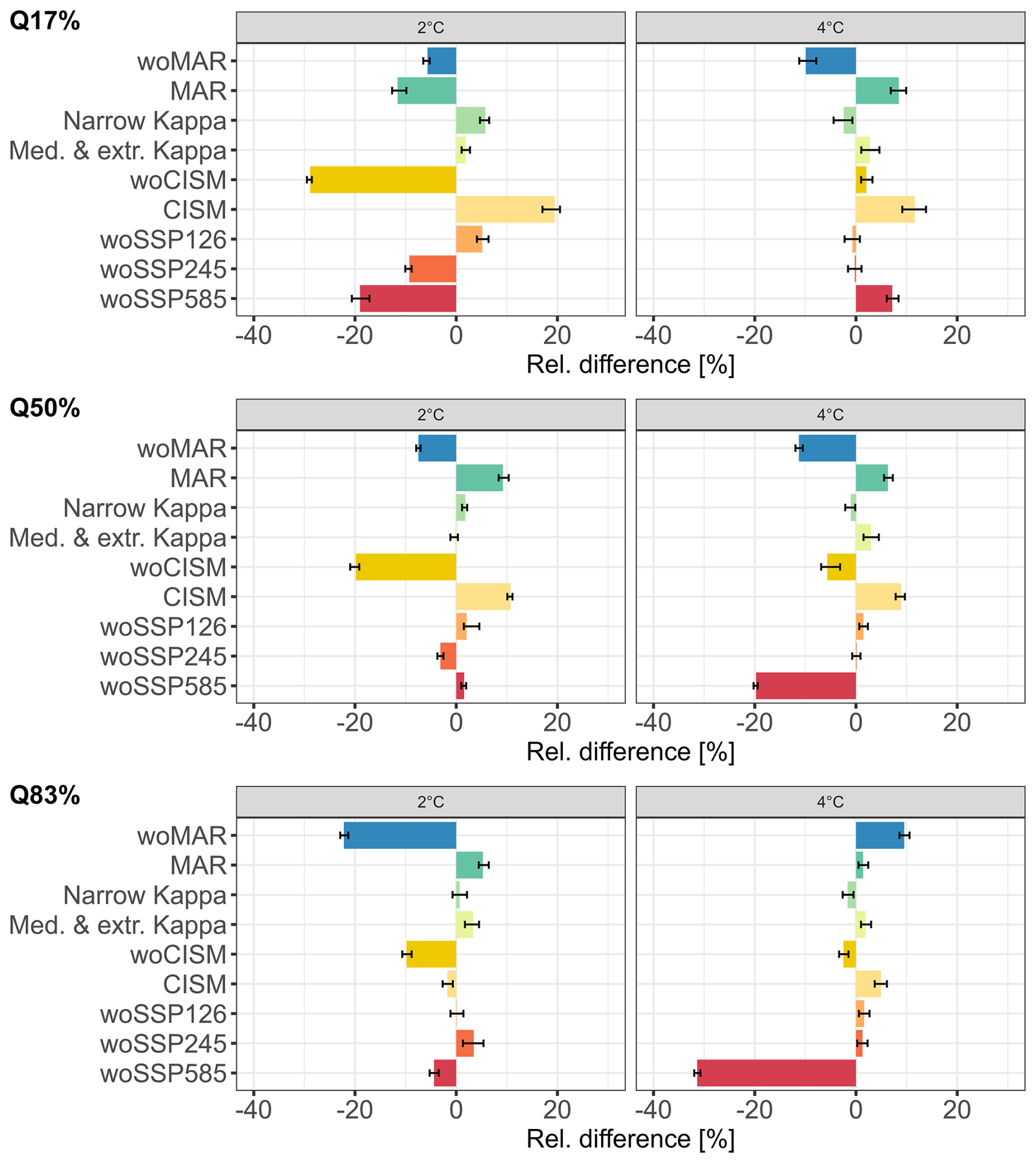
Figure 10 Relative difference (in %) between the RF reference solution and the RF model trained when considering the experiments indicated in the y axis (see Table 2 for full details) for the estimates of three slc percentiles in 2100 relative to 2014, the median and the quantile at 17 % (Q17%) and at 83 % (Q83%), using the random samples generated via the procedure described in Sect. 2.4.2 considering two GSAT changes, 2 °C (±0.5 °C), and 4 °C (±0.5 °C). The endpoints of the error-bars correspond to the 5 % and the 95 % quantiles calculated by applying 100 times the procedure described in Appendix B to reflect the emulator uncertainty.

For the lowest GSAT change scenario, Fig. 10 (left) shows the following results:

• the exclusion of MAR has a significant impact with a particularly high absolute change up to ∼20 % for Q83%;

• the influence of “woCISM” as the percentile level increases goes in oppositive direction compared to “woSSP5-8.5” experiment for the highest GSAT change scenario. The higher the percentile level, the lower the influence of excluding CISM with absolute changes ranging from ∼30 % to ∼5 % when the level increases from 17 % to 83 %;

• for this GSAT change scenario, excluding SSP5-8.5 only substantially influences Q17%, with an absolute change of ∼20 %.

Similarly as for the performance analysis in Sect. 3.2, including a unique ISM, here CISM, or a unique RCM, here MAR, in the MME has a non-negligible influence leading to absolute changes between ∼10 % to ∼20 % mainly for low-to-moderate percentile levels regardless of the GSAT change scenario considered. Overall, the design decision for κ has only a minor impact, which can be considered negligible since its influence is on the same order of the emulator uncertainty indicated by the width of the error-bars for most GSAT change scenarios and percentiles considered with the exception of “Narrow Kappa” experiment for Q17% and GSAT change of 2 °C. This result agrees well with the analysis on the RF predictive capability in Sect. 3.2.

4 Synthesis and Discussion

4.1 Implications for MME design

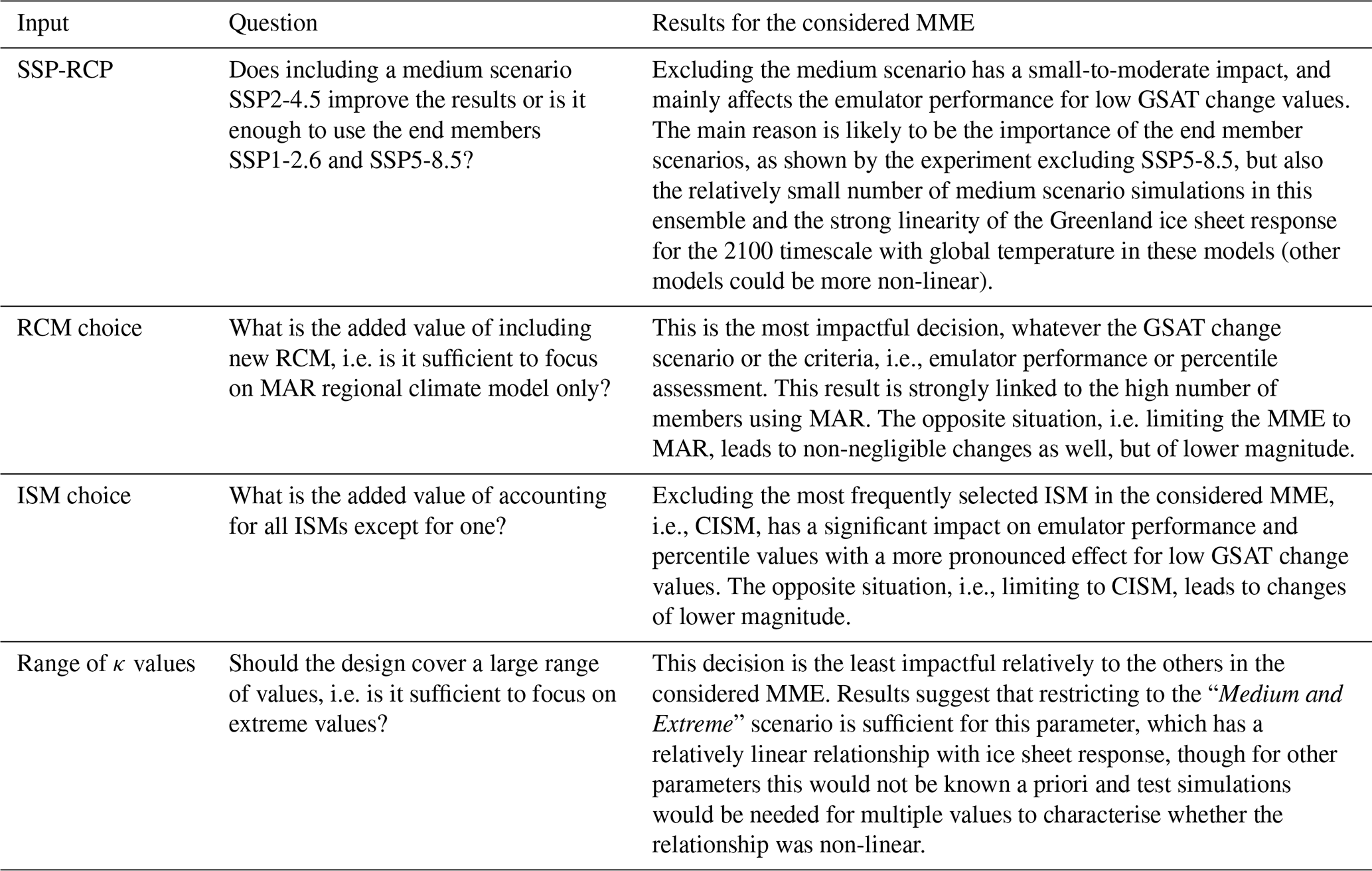
Table 3 summarises the main results from the emulator's experiments for each design question considering the MME of this study. In the following, we take the viewpoint of a MME designer, and derive the practical recommendations from these results.

Table 3 Summary of the results from the emulator's experiments for each design question considering the MME of this study.

On the one hand, some conclusions were expected beforehand, namely the highest influence of the emulator experiment leading to the highest decrease in the MME size of ≈90 %, i.e., “woMAR”. This decrease logically degrades the predictive capability and the reliability of the prediction intervals since the RF is trained on a small dataset (Sect. 3.2). The comparison in Fig. 11a of the slc cumulative distribution function (CDF) of the original MME and that of the reduced MME illustrates the gaps in the training data as indicated by the step-like shape of the CDF. On the other hand, some other conclusions could not necessarily have been anticipated in detail more particularly the implications on the percentile assessment (Sect. 3.3). Our results show that the magnitude of the influence depends on the GSAT change scenario considered, the performance criterion and the target percentile level. For the high GSAT change scenario, the exclusion of SSP5-8.5 has as much impact as the exclusion of MAR on emulator performance, and is even the biggest contributor to changes in the high percentiles. For the low GSAT change scenario, excluding CISM has as much impact as excluding MAR on the emulator performance, and contributes most to changes in the low percentiles. The decrease in MME size induced by “woCISM” and “woSSP585” is smaller than that induced by “woMAR”, on the order of 70 %, suggesting that it is not only a problem of “size” but also a problem of the type of information that is removed from the MME. Figure 11c shows that, when applying “woSSP585” experiment, the emulator is learned with slc spanning a restricted range lower than that of the original MME. This means that the emulator is built with little information on large slc values, and to predict cases associated to high GSAT change scenarios, the RF model mainly relies on extrapolation. This is a situation where emulator methods such as RF can fail completely; see e.g., Buriticá and Engelke (2024). Analysis of Fig. 11a and b helps to understand why “woMAR” and “woCISM” induce roughly equivalent changes for the 2 °C GSAT change scenario, as the slc CDF appears to be similarly disrupted by the application of these experiments with a CDF shifted towards low-to-moderate slc values, particularly in the slc range of ∼5 to ∼15 cm. This means that the emulators are built on members whose slc values span approximately the same range.

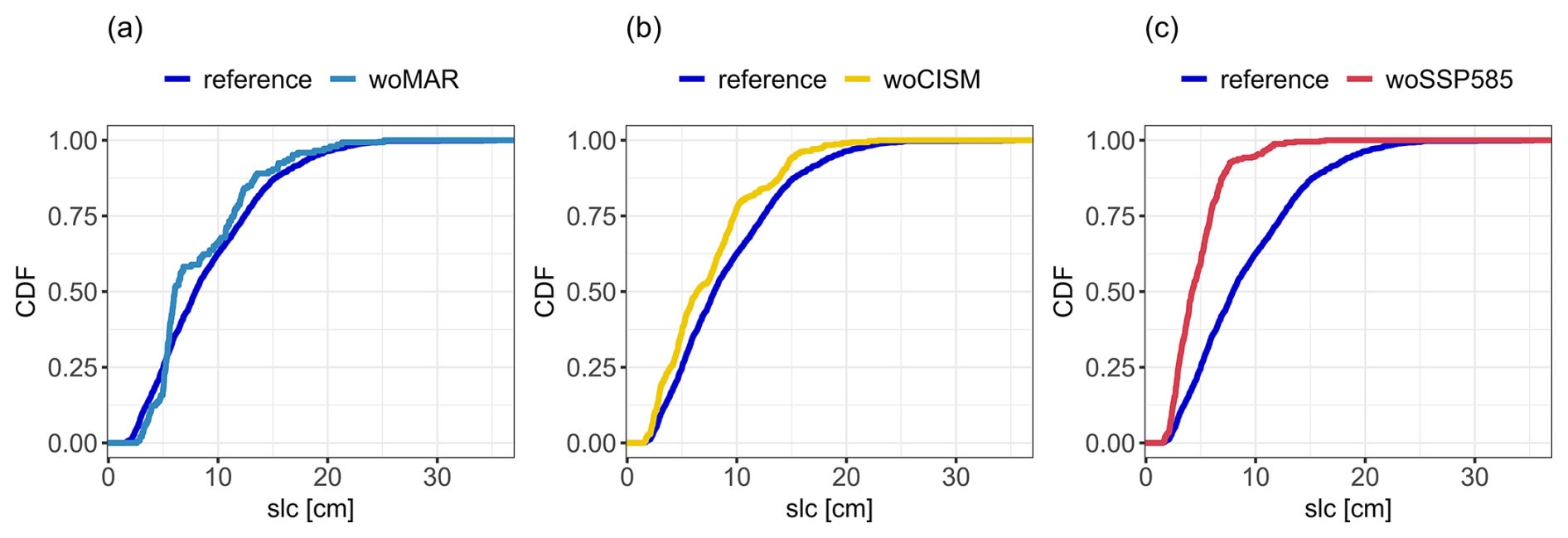
Figure 11 Comparison between the Cumulative Distribution Function (CDF) of slc in 2100 of the original MME (reference) and of the reduced MME after application of the emulator experiments, “woMAR” (a), “woCISM” (b), “woSSP585” (c).

The oppositive experiments that consist in using MME restricted to members to a specific ISM or a particular RCM, here CISM or MAR respectively, are also informative. Although the corresponding emulator experiments imply a reduction of less than 30 % of the MME size, the decline in emulator performance or changes in percentiles cannot be considered negligible. This suggests that removing members associated with other ISMs/RCMs from the training set has an impact, because these members contain information relevant to the RF emulator capability to make predictions, especially in the situations explained in Sect. 2.3, for levels of categorical variables not seen in the training dataset.

The interaction between the reduction in the size of the MME and the type of information important for the training of the emulator is however complex to analyse due to the multiple joint effects to be taken into account between the inputs. Analysis of Fig. 11 reveals certain similarities in the effect of the different emulation experiments, but is not sufficient to explain all aspects of the problem; for example, this type of analysis does not fully explain why “woCISM” has a stronger impact on performance at GSAT change of 2 °C than 4 °C. From a methodological viewpoint, this calls for further developments, in particular by relying on the data valuation domain (Sim et al., 2022). These types of tools aim to study the worth of data in machine learning models based on similar methods as the ones used by Rohmer et al. (2022) in the context of sea level projections. Transposed to the MME context, these tools could be used in future studies to assess the impact of each member in the emulator's predictions, i.e. the worth of each member. From a broader perspective on collaborative research, our results on the influence of RCM and ISM models can be seen as an additional justification for intensifying the model intercomparison efforts initiated in the past, in particular ISMIP6 (Nowicki et al., 2016), which included coupled ISMs as well as stand-alone ISMs in CMIP for the first time. They also support, to some extent, a posteriori, the choices that have been made for the construction of the MME considered here (based on Goelzer et al., 2020).

Finally, a very practical implication can be derived from the κ experiments: results indicate that restricting to the extreme and medium scenario is sufficient here because of the lesser impact between the two experiments, “Med. & Extr.” or “Narrow”. This result is interpreted as being linked to a quasi-linear relationship between κ and slc as shown in Rohmer et al. (2022) using the MME of ISMIP6 for Greenland. This was confirmed by the analysis detailed in Sect. S3. In practice, this result implies that the number of scenarios explored in the MME can be limited to a three-scenario approach (low-medium-high value), i.e. the number of members can be reduced, thus reducing the number of long numerical simulations required.

4.2 Implications from stakeholders' point of view

Our work can help stakeholders in several ways. First, our study contributes to a better understanding of the estimated contribution of Greenland ice sheet melting to sea level rise. According to the latest authoritative sea level projections developed by the IPCC (Fox-Kemper et al., 2021) the GIS contribution to sea level rise is projected to reach 8 cm [4; 13] (median [likely range]) by 2100 for the SSP2-4.5 scenario. This means Greenland has a sizeable share to the total global mean sea level rise and their uncertainties, which were estimated at 56 cm [44; 76] for this scenario according to the same report. Here, we showed that some choices made by modelers, such as the tidewater glacier retreat parameter, have a minor impact on the spread of the Greenland sea level rise contribution, whereas others, such as using only MAR as RCM, have a large impact. These findings can be useful to inform future modelling experiments, and could help identifying where modelling efforts could focus to better characterize the spread of the projected contribution of the Greenland ice-sheet and to increase our understanding of that spread. Second, our results support coastal adaptation practitioners in their decision-making. Our emulator experiments in Sect. 3.2 and 3.3 highlight how the different modelling choices affect differently the median or the upper tail (here measured by the Q83% percentile). This difference is important, because the literature on adaptation decision-making has clearly shown that knowing the median is not sufficient for coastal adaptation practitioners managing long-living critical infrastructures or making strategic decisions for regions or countries (Hinkel et al., 2019). These practitioners need credible assessments of the uncertainties in ice mass losses in Greenland, including for the low probability scenarios corresponding to the tail of probabilistic projection. For example, France selected a unique climate scenario of 3 °C GWL used in France within its 3^rd development plan published in 2025. To define the associated sea level scenarios to be mainstreamed in public policies, a detailed consideration of uncertainties is required to understand which security margins are taken (Le Cozannet et al., 2025). Thus, our study supports the need for improved experimental designs by making some practical recommendations, especially regarding the consideration of ISM, RCM and RCP8.5/SSP5-8.5 simulations.

Finally, the importance of SSP5-8.5, although expected, also underlines the fact that a wide range of emissions scenarios and climate simulations should continue to be considered in the future. The SSP5.8-5 scenario in this ensemble contains many simulations and covers a wide range of global warming levels at 2100. To represent plausible outcomes of failure of states to meet their own commitments, or political backlashes leading to climate policy setbacks (see recent discussion by Meinshausen et al., 2024), medium and medium-high emissions scenarios (e.g. radiative forcing reaching between 4.5 and 7.0 W m⁻² in 2100) should continue to be used for simulations of climate impacts such as for the Greenland ice sheet, so that these do not rely too much on emulators interpolating from end member scenarios. Furthermore, the current design of the SSP3-7.0 involves very high aerosol emissions, so that the resulting simulations need to be considered carefully (Shiogama et al., 2023). Being able to use more intermediate climate simulations reaching radiative forcing between 4.5 and 7.0 W m⁻² in 2100 is all the more important as another need is now emerging: projections of ice mass loss for specific levels of global warming relative to preindustrial (as in the IPCC: Fox-Kemper et al., 2021). For example, the latest adaptation plan in France requires adaptation practitioners to test their adaptation measures against a climate change scenario reaching 2 °C in 2050 and 3 °C in 2100 globally (Le Cozannet et al., 2025). Motivations for considering these GWLs rather than SSP or RCP scenarios include their perceived clarity for a wide range of adaptation practitioners, as well as the direct links that can be made with the climate objectives set out in the Paris agreement to stabilize climate change well below 2 °C GWL. For all scenarios, including global warming levels, the development of probabilistic projections requires emulators, whose accuracy and precision can be improved by better experimental design.

5 Concluding remarks and further work

Developing robust protocols to design balanced and complete numerical experiments for MME is a matter of active research that has called for multiple studies either for sea level projections via selection criteria (Barthel et al., 2020) or from an uncertainty assessment's perspective (Aschwanden et al., 2021), and more generally for regional impact assessment (Evin et al., 2019; Merrifield et al., 2023). In this study, we took advantage of a large MME produced for Greenland ice sheet contributions to future sea level by 2100 to define a series of emulator's experiments that are closely related to practical MME design decisions. Our results confirm the high importance of including the SSP5-8.5 scenario in terms of emulator performance and percentile estimates. They also show that an ensemble designed only with a unique ISM and RCM model, i.e., here with the one that is most frequently selected in the considered MME, has non-negligible implications. These results point to the size of the training set as the key driver of the changes in the emulator performance and percentile estimates, hence underlying the need for building large ensembles to develop accurate and reliable emulators. Broad participation in projects such as ISMIP, with as many simulations as possible contributed by numerous groups, appears to be an effective option to this end. Finally, the less impactful choice in this ensemble is the one in the sampling of the Greenland tidewater glacier retreat parameter, because it has a relatively linear relationship with sea level contribution. These recommendations (detailed in Table 3) can be informative for the design of next generation MME for Greenland (ISMIP7: Nowicki et al., 2023).

Although the MME considered in this study covers a large spectrum of situations (multiple SSP scenarios, different RCMs and ISMs), with more than 1,000 members, a series of aspects need to be considered in the future to further increase the robustness of these results. First, our procedure should be tested on additional MMEs of interest to improve the transferability of our results, in particular for Antarctica (Seroussi et al., 2020), for multi-centennial projections (e.g., Seroussi et al., 2024), and for glaciers (Marzeion et al., 2020). These tests should also include new types of MMEs that are combined with calibration (e.g., Aschwanden and Brinkerhoff, 2022). They make it possible to circumvent an assumption in our study, namely that all members have the same weight, by taking into account the reliability of the different members or observational constraints, provided that good-quality data are available over a sufficiently long period in the past and that the numerical implementation of the ISMs is suitable for calibration. To address this question, a wider range of uncertainties should be considered, more specifically model and structural uncertainties (i.e., uncertainty in the formulation of the model and its ability to represent the physics of the system), in addition to uncertainties in model parameters (related to ice dynamics and atmospheric/oceanic forcing), but also irreducible uncertainties such as internal climate variability as investigated by Verjans et al. (2025) on Greenland sea level contribution projections. Here, emulators are expected to play a key role to explore this wide uncertain space thoroughly.

Second, our results are based on the use of an emulator, i.e., a statistical approximation of the “true” chain of numerical models. The RF emulator trained in our study showed satisfactory predictive capabilities for low and high levels of warning (GSAT changes of respectively 2 and 4 °C). The emulator performance remained however unsatisfactory at intermediate levels of warming (3 °C). Despite, the efforts made in our study to nuance the results by including indicators of the emulator uncertainty, the emulator training should be improved in the future by considering alternative emulator models (e.g., Yoo et al., 2025) but also more robust approaches for hyperparameter tuning (Bischl et al., 2023), and more particularly more advanced categorical variables' encoding (Au, 2018; Smith et al., 2024), which is key to apply the proposed emulator experiments.

Finally, our recommendations are derived, by construction, a posteriori, i.e., based on the available members of a large-size MME. Therefore, a third avenue here is to derive recommendations earlier on in the process, i.e., early during the construction of the MME design. This could be done iteratively. The procedure could alternate between simulation phases, i.e. either test simulations to assess sensitivity to different inputs, or small exploratory sets that do not use all the available computing time/human/project resources, and training and retraining of the emulator.

Appendix A: Random Forest regression model

Let us first denote slc${}_{i=\mathrm{1},\mathrm{\dots },n}$ the ith value of sea level contribution calculated relative to the ith vector of p input parameters' values ${\mathit{x}}_{i=\mathrm{1},\mathrm{\dots },n}=\mathit{\{}{x}_{\mathrm{1}},x_{\mathrm{2}},\mathrm{\dots },x_p{\mathit{\}}}_{i=\mathrm{1},\mathrm{\dots },n}$ where n is the total number of experiments. The Random Forest (RF) regression model is a non-parametric technique based on a combination (ensemble) of tree predictors (using regression tree, Breiman et al., 1984). By construction, tree models can deal with mixed types of variables, categorical or continuous. Each tree in the ensemble (forest) is built based on the principle of recursive partitioning, which aims at finding an optimal partition of the input parameters' space by dividing it into L disjoint sets R₁, …, R_L to have homogeneous slc_i values in each set $R_{l=\mathrm{1},\mathrm{\dots },L}$ by minimizing a splitting criterion, which is chosen in this study as the sum of squared errors (Breiman et al., 1984). The minimal number of observations in each partition is termed nodesize (denoted “ns”).

The RF model, as introduced by Breiman (2001), aggregates the different regression trees as follows: (1) random bootstrap sample from the training data and randomly select m_try variables at each split; (2) construct n_tree trees T(α), where α_t denotes the parameter vector based on which the tth tree is built; (3) aggregate the results from the prediction of each single tree to estimate the conditional mean of slc as:

$$\begin{array}{}\text{(A1)}& E\left(\mathrm{slc}\right|\mathbf{X}=\mathit{x})=\sum _{j=\mathrm{1}}^n{w}_j(\mathit{x}){\mathrm{slc}}_j,\end{array}$$

where E is the mathematical expectation, and the weights w_j are defined as

$$\begin{array}{}\text{(A2)}& \begin{array}{rl}& w_j\left(\mathit{x}\right)={\displaystyle \frac{\sum _{t=\mathrm{1}}^{n_{\mathrm{tree}}}{w}_j(\mathit{x},{\mathit{\alpha }}_t)}{n_{\mathrm{tree}}}},\\ & \text{with }{w}_j(\mathit{x},\mathit{\alpha })={\displaystyle \frac{I_{\left\{X_j\mathit{ϵ}{R}_{l(x,\mathit{\alpha })}\right\}}}{\mathit{\#}\left\{i:X_i\mathit{ϵ}{R}_{l(x,\mathit{\alpha })}\right\}}},\end{array}\end{array}$$

where I_{A} is the indicator operator which equals 1 if A is true, 0 otherwise; R_l(x,α) is the partition of the tree model with parameter α which contains x.

The RF hyperparameters considered in the study are ns and m_try which have shown to have a large impact on the RF performance (Probst et al., 2019). To select values for these parameters, we rely on an approach based on a 10-fold cross validation exercise (Hastie et al., 2009), which consists in varying ns from 1 to 10, and m_try from 1 to 7, and in selecting the most optimal combination with respect to cross-validation predictive error. The number of random trees is fixed at 1000; preliminary tests having showed that this latter parameter has little influence provided that it is large enough.

An additional difficulty of our study is the presence of a large number of categorical variables with large number of levels (unordered values). The partitioning algorithm described above tends to favour categorical predictors with many levels (Hastie et al., 2009: Chap. 9.2.4). To alleviate this problem, we rely on the computationally efficient algorithm proposed by Wright and König (2019) based on ordering the levels a priori, here by their slc mean response.

Appendix B: Accounting for the emulator uncertainty

The RF method described in Appendix A is very flexible and can be adapted to predict quantiles, which can be used to assess the RF emulator uncertainty. To do so, we rely on the quantile regression forest (qRF) model, which was originally developed by Meinshausen (2006), who proposed to estimate the conditional quantile τq(slc|x) at level τ as

$$\begin{array}{}\text{(B1)}& q^{\mathit{\tau }}\left(\mathrm{slc}\mathrm{|}\mathit{x}\right)=\inf (\mathit{x}:F_{\mathrm{SLC}\mathrm{|}\mathbf{X}}(\mathrm{slc}\mathrm{|}\mathit{x})\ge \mathit{\tau }),\end{array}$$

where inf(.) is the infimum function, and,

$$\begin{array}{}\text{(B2)}& F_{\mathrm{SLC}\mathrm{|}\mathbf{X}}\left(\mathrm{slc}\mathrm{|}\mathit{x}\right)=\sum _{j=\mathrm{1}}^n{w}_j\left(\mathit{x}\right)I_{\left\{{\mathrm{slc}}_j\le \mathrm{slc}\right\}},\end{array}$$

where the weights are calculated in the same manner as for the regression RF model (described in Appendix A). The major difference with the formulation for regression RF is that the qRF model computes a weighted empirical cumulative distribution function of slc for each partition instead of computing a weighted average value.

The quantiles computed using the qRF model can directly be used to define the prediction intervals at any level α: $\text{PI}\left({\mathit{x}}^{\ast }\right)=\left[q^{\frac{\mathit{\alpha }}{\mathrm{2}}}\left(\mathrm{slc}\mathrm{|}{\mathit{x}}^{\ast }\right);q^{\mathrm{1}-\frac{\mathit{\alpha }}{\mathrm{2}}}\left(\mathrm{slc}\mathrm{|}{\mathit{x}}^{\ast }\right)\right]$, which can be used to reflect the RF emulator uncertainty when providing the emulator predictions.

When performing the probabilistic predictions (Sect. 2.4.2), the emulator uncertainty is propagated in addition to the uncertainty of the different input variables based on the following procedure:

Step 1. Draw N random realizations of the input variables $\stackrel{\mathrm{̃}}{x}$;

Step 2.1. Draw N random number $\stackrel{\mathrm{̃}}{u}$ between 0 and 1 by assuming a uniform random distribution;

Step 2.2. Approximate the cumulative distribution function of $\mathrm{slc}\mathrm{|}\stackrel{\mathrm{̃}}{x}$ by computing the N values $\stackrel{\mathrm{̃}}{\mathrm{slc}}=q^{\stackrel{\mathrm{̃}}{u}}\left(\mathrm{slc}\mathrm{|}\stackrel{\mathrm{̃}}{x}\right)$ given $\stackrel{\mathrm{̃}}{u}$ and $\stackrel{\mathrm{̃}}{x}$ using the qRF model;

Step 2.3. Compute the quantile Q^τ at the chosen level τ from the set of N values of $\stackrel{\mathrm{̃}}{\mathrm{slc}}$. The range $\left[Q^{\frac{\mathit{\alpha }}{\mathrm{2}}};Q^{\mathrm{1}-\frac{\mathit{\alpha }}{\mathrm{2}}}\right]$ then provides the 1−α confidence interval of the emulator prediction for $\left(\mathrm{slc}\mathrm{|}\stackrel{\mathrm{̃}}{x}\right)$;

Step 3. Repeat N₀ times Steps 2.1 to 2.3. At Step 2.2, $\stackrel{\mathrm{̃}}{slc}$ are calculated for the same set of random input variables $\stackrel{\mathrm{̃}}{x}$ defined at Step 1, but each time a newly randomly generated set of levels $\stackrel{\mathrm{̃}}{u}$ is used based on Step 2.1. This means that, at Step 2.3, the newly calculated quantiles Q^τ vary for each of the repetitions.

The output of the procedure is a set of N₀ quantile values $(Q_{\left(\mathrm{1}\right)}^{\mathit{\tau }},Q_{\left(\mathrm{2}\right)}^{\mathit{\tau }},\mathrm{\dots },Q_{\left(N_{\mathrm{0}}\right)}^{\mathit{\tau }})$. The variability among these values reflects the emulator uncertainty and can be summarized by the 1−α % confidence interval with lower and upper bounds defined by the $\mathit{\alpha }/\mathrm{2}$, and the $\mathrm{1}-\mathit{\alpha }/\mathrm{2}$ quantile of Q^τ. In this study, we choose N=10,000, N₀=100 and α=10 %.

Appendix C: Screening analysis

We rely on the hypothesis testing of Altmann et al. (2010). To identify the significant predictor variables, the null hypothesis “no association between slc and the corresponding predictor variable” is tested. The corresponding p value is evaluated by (1) computing the probability distribution of the importance measure of each predictor variable through multiple replications (here 1000) of permuting slc; (2) training a RF model; and (3) computing the permutation-based variable importance. In this procedure, the p values quantify how unlikely the variable importance in the non-permuted data is with respect to the null distribution of variable importance reached from the permutations. In practice, when the p value is below a given significance threshold (typically of 5 %), it indicates that the null hypothesis should be rejected, i.e., the considered predictor variable has a significant influence on slc. Figure C1 shows that four predictor variables have non-significant influence with p values above 5 %, namely the choice in the account for thermodynamics, the choice in the sliding law, the type of initialisation and the number of years for initialisation phase.

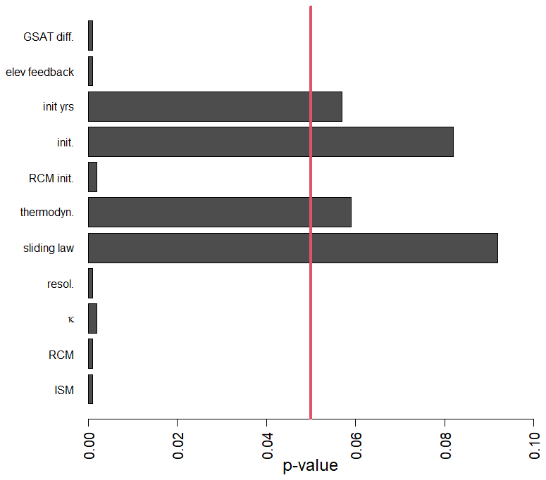
Figure C1 Screening analysis showing the p values of the RF variable importance-based test of independence of Altmann et al. (2010). The vertical red line indicates the significance threshold at 5 %. When the p value is below 5 %, it indicates that the null hypothesis should be rejected, i.e., the considered variable has a significant influence, and should be retained in the RF construction.

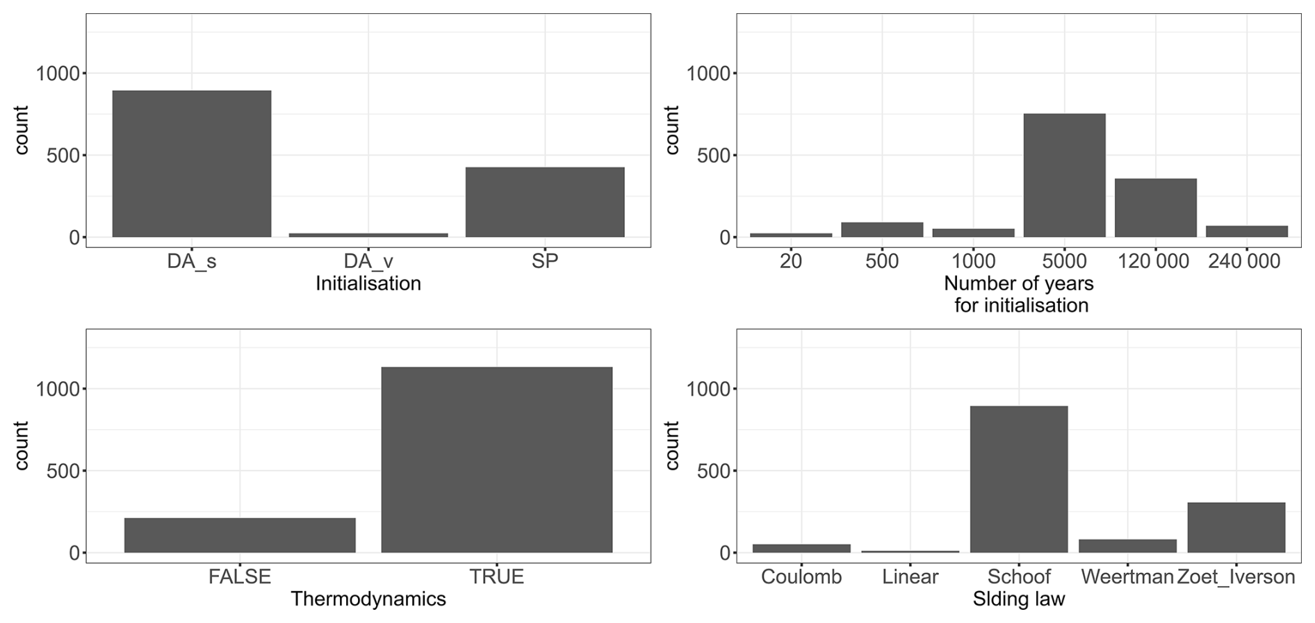
Figure C2 Count number of the MME members with respect to the variables identified as non-influential.

Appendix D: Formal definition of the performance criteria

Let us consider the slc prediction error, i.e. $e^{\left(i\right)}={\mathrm{slc}}^{\left(i\right)}-{\widehat{\mathrm{slc}}}^{\left(i\right)}$ for each test sample i=1, …, n_test with $\widehat{\mathrm{slc}}$ the mean value provided by the RF model (see Appendix A). We consider the following performance criteria:

• the relative absolute error (quoted as a percentage),

  $$\begin{array}{}\text{(D1)}& \text{RAE}={\displaystyle \frac{\mathrm{1}}{n_{\mathrm{test}}}}\sum _{i=\mathrm{1}}^{n_{\mathrm{test}}}\left|{\displaystyle \frac{e^{\left(i\right)}}{{\mathrm{slc}}^{\left(i\right)}}}\right|,\end{array}$$

• the coefficient of determination,

  $$\begin{array}{}\text{(D2)}& Q^{\mathrm{2}}=\mathrm{1}-{\displaystyle \frac{\sum _{i=\mathrm{1}}^{n_{\mathrm{test}}}{\left(e^{\left(i\right)}\right)}^{\mathrm{2}}}{\sum _{i=\mathrm{1}}^{n_{\mathrm{test}}}{\left({\mathrm{slc}}^{\left(i\right)}-\stackrel{\mathrm{‾}}{\mathrm{slc}}\right)}^{\mathrm{2}}}}\end{array}$$

  where $\stackrel{\mathrm{‾}}{\mathrm{slc}}$ is the average value of slc calculated over the test set;

• the continuous rank probability score CRPS, that jointly quantifies the calibration of qRF probability distribution, i.e. the reliability of the estimation, and its sharpness (i.e. the concentration/dispersion of the probability distribution). To evaluate CRPS, the formulation based on quantiles (Bracher et al., 2021: Sect. 2.2) is used:

  $$\begin{array}{}\text{(D3)}& \begin{array}{rl}\text{CRPS}& =\mathrm{2}\underset{\mathrm{0}}{\overset{\mathrm{1}}{\int }}B(q^{\mathit{\tau }}\left(\mathrm{slc}\mathrm{|}{\mathit{x}}^{\ast }\right),{\mathrm{slc}}^{\mathrm{true}})\mathrm{d}\mathit{\tau }\\ & \approx {\displaystyle \frac{\mathrm{2}}{P}}\sum _{\mathit{\tau }\in \mathrm{\Gamma }}B\left(q^{\mathit{\tau }}\left(\mathrm{slc}\mathrm{|}{\mathit{x}}^{\ast }\right),{\mathrm{slc}}^{\mathrm{true}}\right)\end{array}\end{array}$$

  where the term $\mathit{\tau }B\left(q^{\mathit{\tau }}\left(\mathrm{slc}\mathrm{|}{\mathit{x}}^{\ast }\right),{\mathrm{slc}}^{\mathrm{true}}\right)$ is the quantile loss function and defined as:

  $$\left\{\begin{array}{ll}\left(\mathrm{1}-\mathit{\tau }\right)\left(q^{\mathit{\tau }}\left(\mathrm{slc}\mathrm{|}{\mathit{x}}^{\ast }\right)-{\mathrm{slc}}^{\mathrm{true}}\right)& \text{if }{\mathrm{slc}}^{\mathrm{true}}<q^{\mathit{\tau }}\left(\mathrm{slc}\mathrm{|}{\mathit{x}}^{\ast }\right)\\ \mathit{\tau }\left({\mathrm{slc}}^{\mathrm{true}}-q^{\mathit{\tau }}\left(\mathrm{slc}\mathrm{|}{\mathit{x}}^{\ast }\right)\right)& \text{if }{\mathrm{slc}}^{\mathrm{true}}\ge q^{\mathit{\tau }}\left(\mathrm{slc}\mathrm{|}{\mathit{x}}^{\ast }\right)\end{array}\right.,$$

  where slc^true is the true value of the sea level contribution, and where the quantiles q^τ(slc|x^∗) are evaluated using the trained qRF model at given instance of the input variables x^∗ for an equidistant dense grid of quantile levels $({\mathit{\tau }}_{\mathrm{1}},\mathrm{\dots },{\mathit{\tau }}_P)$ with ${\mathit{\tau }}_i<{\mathit{\tau }}_{i+\mathrm{1}}$ and ${\mathit{\tau }}_{i+\mathrm{1}}-{\mathit{\tau }}_i=\mathrm{1}/P$. In this study, we consider level τ₁=5 % and τ_P=95 % with $\mathrm{1}/P=\mathrm{5}$ %.

• the coverage αCA¹⁻ of the prediction intervals PI^α at significance level α defined as

  $$\begin{array}{}\text{(D4)}& {\text{CA}}^{\mathrm{1}-\mathit{\alpha }}={\displaystyle \frac{\mathrm{1}}{n_{\mathrm{test}}}}\sum _{i=\mathrm{1}}^{n_{\mathrm{test}}}{I}_{\mathit{\{}{\mathrm{slc}}_i\in {\mathrm{PI}}^{\mathit{\alpha }}\left({\mathit{x}}^i\right)\mathit{\}}},\end{array}$$

  where I_{A} is the indicator function. CA^1−α evaluates the proportion of “true” slc that fall within the bounds of the prediction interval. The interval PI^α is well calibrated when CA^1−α is close to the theoretical value of 1−α;

• the inter-quartile ratio ${\text{iqr}}_i=\left(q^{\mathrm{0.75}}\left(\mathrm{slc}\mathrm{|}{\mathit{x}}^{\ast }\right)-q^{\mathrm{0.25}}\left(\mathrm{slc}\mathrm{|}{\mathit{x}}^{\ast }\right)\right)/\text{RMSE}$ for the ith element of the test set (Bellon-Maurel et al., 2010). This ratio allows to assess whether the emulator prediction uncertainty measured by the difference $q^{\mathrm{0.75}}\left(\mathrm{slc}\mathrm{|}{\mathit{x}}^{\ast }\right)-q^{\mathrm{0.25}}\left(\mathrm{slc}\mathrm{|}{\mathit{x}}^{\ast }\right)$ is on the same order than the prediction error measured by the root mean square error $\text{RMSE}=\sqrt{\frac{\mathrm{1}}{n_{\mathrm{test}}}\sum _{i=\mathrm{1}}^{n_{\mathrm{test}}}(e^{\left(i\right)}{)}^{\mathrm{2}}}$. If iqr <1 (>1), this indicates over- (under-) confidence in the emulator prediction. An aggregated score is defined as:

  $$\begin{array}{}\text{(D5)}& \text{IQR}={\displaystyle \frac{\mathrm{1}}{n_{\mathrm{test}}}}\sum _{i=\mathrm{1}}^{n_{\mathrm{test}}}\left({\text{iqr}}_i\right)\end{array}$$

Appendix E: List of acronyms/abbreviations

AR	Assessment Report
CMIP	Coupled Model Intercomparison Project
CRPS	Continuous Ranked Probability Score
GCM	Global Climate Model
GrIS	Greenland Ice-Sheet
GSAT	Global Surface Atmosphere Temperature
GWL	Global Warming Level
IPCC	Intergovernmental Panel on Climate Change
IQR	Ratio of performance to the interquartile distance
ISM	Ice-Sheet Model
ISMIP	Inter-Sectoral Impact Model Intercomparison Project
PI	Prediction interval
qRF	Quantile Random Forest
MME	Multi-model ensemble
RAE	Relative Absolue Error
RCM	Regional Climate Model
RCP	Representative Concentration Pathway
RF	Random Forest
RMSE	Root Mean Square Error
slc	Sea level contribution
SMB	Surface Mass Balance
SSP	Shared Socio-economic Pathways