Sea ice concentration estimates from ICESat-2 linear ice fraction – Part 2: Gridded data comparison and bias estimation

Sea ice coverage is a key indicator of changes in the global climate. Estimates of sea ice area and extent are primarily derived from satellite measurements of surface microwave emissions, from which local sea ice concentration (SIC) is derived. Passive microwave (PM) satellite sensors remain the sole global product for understanding SIC variability but may be sensitive to consistent biases. In Part I (Buckley et al., 2025) we explored these in a multi-sensor intercomparison of optical, passive microwave, and lidar data, showing that a new SIC product, the linear ice fraction (LIF), derived from ICESat-2 (IS2) laser altimetry, could be used to quantify and understand PM SIC biases. Here in Part II, we develop and assess the reliability of larger-scale estimates of SIC from IS2 LIF. We develop an LIF emulator that samples optical imagery using the distribution of possible orientation angles for IS2 to understand the limitations of this one-dimensional product. We find that the error qualities of the LIF product are improved when combining multiple IS2 tracks and discuss intrinsic but correctable biases that emerge in the combination of multiple IS2 measurements. We use these to develop a monthly LIF product, covering up to 46 % of the Arctic sea ice cover, which has similar or better error qualities compared to PM data, subject to uncertainties in surface-type classification associated with surface melting and differences between IS2's weak and strong beams. We then discuss pathways to improving LIF and enhancing PM-SIC data in the future.

1 Introduction

Sea ice concentration (SIC), the fraction of an ocean area covered by sea ice, is critically important for understanding polar climate variability. SIC is estimated globally using passive microwave (PM) satellites at both hemispheres, with PM-derived SIC the standard for assessing sea ice state and change (Meredith et al., 2022). Increasingly, SIC products are assimilated into state-of-the-art forecast and climate models at both hemispheres (Mazloff et al., 2010; Sakov et al., 2012; Massonnet et al., 2015; Verdy and Mazloff, 2017; Fritzner et al., 2019; Zhang et al., 2021), making potential improvements in global SIC observations important for accurate climate analysis and prediction. Local errors in PM SIC are observed to have a compensating effect when integrated over the Arctic or Antarctic; hence the impact of algorithmic uncertainty or bias on estimates of total (Arctic or Antarctic) sea ice area is estimated to be small, even in summer (Notz, 2015; Meier and Stewart, 2019; Kern et al., 2020). Still, no remote sensing alternatives to PM exist for measuring SIC from local to global scales that do not require information about the PM signature of sea ice.

In Part 1 of this two-part study (Buckley et al., 2025), we compared daily retrievals from state-of-the-art PM sensors and PM-SIC algorithms against high-resolution optical data from NASA's Operation IceBridge (OIB). We calculated SIC from optical imagery by applying a surface-type classification algorithm (Buckley et al., 2020) to the images, defining each pixel as open water, sea ice, or melt pond, and determined a sea ice concentration for each ∼  400 m by ∼  600 m image. We found that PM-SIC products demonstrated consistent positive biases (1 %–6 %) over compact sea ice, potentially because of the presence of small crack features in the sea ice mosaic that cover a limited portion of the overall surface and are challenging to capture with large PM grid sizes (6.25 to 25 km cells), similar to findings in related studied of PM-SIC and optical data (Kern et al., 2019). However, these fractures may contribute greatly to air–sea exchange. This intercomparison showed a wide uncertainty range for PM-SIC summer months (May–September) because of the well-known challenges in retrieval of SIC over ponded sea ice. Part I includes details of these biases and limitations of PM products.

We showed in Part I that NASA's ICESat-2 satellite (IS2) can be used to develop a linear SIC estimate, which we call the linear ice fraction (LIF), which has reduced or similar bias compared to PM over a set of imagery coincident with IS2 overflights in Arctic winter conditions. IS2 is a photon-counting laser altimeter with 0.7 m along-track sampling, an 11 m footprint, and high skill in differentiating sea ice and open water in non-summer months (Farrell et al., 2020; Kwok et al., 2020, 2021). IS2 can resolve Arctic leads at the meter scale (Petty et al., 2021; Kwok et al., 2021), especially in winter, when leads are the primary source of air–sea exchange. The geographic extent of LIF can depend on PM SIC because ATL07 segments are only produced in regions where SIC from the NSIDC Climate Data Record (Meier et al., 2021) exceeds 15 %. LIF itself is derived exclusively from the classification of IS2 photon returns (at a wavelength of 532 nm) and does not rely on microwave emissions (wavelengths on the order of 1 cm) or related algorithms and therefore has independent and separate uncertainties from PM SIC. Such uncertainties are presently unconstrained and, thus, potentially larger than PM-SIC products, which are the focus of this work.

Here we explore error bounds with IS2 LIF and the possibility of using multiple consecutive IS2 passes to build a gridded LIF product on monthly timescales. We first discuss the uncertainties that will arise when building an IS2-derived gridded product. To understand them, we develop an IS2 emulator which we apply to the optically classified sea ice data explored in Buckley et al. (2025) in Sect. 2.1, using it to derive bounds on how unsupervised errors in SIC retrieval decay as a function of the number of intersections of the sea ice surface by IS2.

Using the error bounds obtained from emulation, in Sect. 3, we build a monthly Arctic LIF product that covers roughly 60 % of Arctic seasonal sea ice extent and explore differences between it and a set of commonly used PM-SIC products at different resolutions. Over these areas, PM SIC is approximately 3 %–4 % higher in non-summer months, with LIF estimating approximately twice as much open water than PM-SIC products, similar to what was obtained from optical comparisons. Finally, we explore prospects for improving LIF skill and how, either in single IS2 passes or as a gridded product, it could be used to augment existing PM SIC data in Sect. 4.

2 ICESat-2 and the linear ice fraction

IS2 is a six-beam laser altimeter with high precision and skill in retrieving sea ice properties (e.g., Kwok et al., 2019a). In this work, and in Buckley et al. (2025), we use Version 6 of the sea ice height product, ATL07, which generates along-satellite-track “segments” from collections of sequential 150 photons (Kwok et al., 2023). Based on the statistical properties of such photons retrievals, each segment is identified with a surface type (water, ice, or cloud covered) (Kwok et al., 2019b). These segments are provided in locations where the local daily NSIDC-CDR sea ice concentration exceeds 15 % and their length averages ∼ 15 m for the three strong beams and ∼ 60 m for the three weak beams (Kwok et al., 2019a).

For any collection of measured IS2 segments, we define the IS2 linear ice fraction (LIF) as

$$\begin{array}{}\text{(1)}& \mathrm{LIF}=\mathrm{100}\times {\displaystyle \frac{\text{length of ice segments}}{\text{length of all surface segments}}}.\end{array}$$

We represent the LIF as a percentage for consistency with typical usage of SIC data. The details of the ATL07 segment-type classification can be found in the Algorithm Theoretical Basis Document (Kwok et al., 2019a), and we follow the preprocessing methods in Horvat et al. (2020b). We exclude all cloud segments, sections with fewer than two segments within 1 km along track, and all segments over 200 m long. Although LIF is calculated with a high-precision instrument and not subject to the passive microwave biases in SIC determination, we note other independent sources of uncertainty.

U1: Classification uncertainty.

The construction of LIF relies upon the IS2 ATL07 classification of along-track segments of the ice-ocean surface as being ice or two types of open water: “specular” leads and “dark” leads. Uncertainty and errors in the ice-water discrimination, which is higher in summer due to the presence of meltwater on the ice surface (Tilling et al., 2020; Farrell et al., 2020; Koo et al., 2023), could lead to systematic error in LIF calculations.

U2: Orientation uncertainty.

The relative orientation of near-linear features in the sea ice mosaic is unknown with respect to the satellite path. While the local azimuth of the IS2 satellite is constrained as a function of latitude (see Fig. 1 and Sect. 2.1), the orientation of sea ice features is not. This can distort the fraction of the observed surface that is ice or open water if the alignment of cracks and IS2 ground tracks is correlated (Rothrock and Thorndike, 1984; Horvat et al., 2020a; Hell and Horvat, 2024).

U3: Coverage uncertainty.

PM satellite products yield daily SIC observations, even in cloudy conditions. IS2, however, makes approximately 15 orbits each day, with its six beams covering a region approximately 6.6 km across, and its photons do not reach the sea ice surface through optically thick clouds. IS2 cannot produce specific measurements of the sea ice surface at any one location at the daily or twice-daily repeat time of PM satellites. Gridded products can only therefore be formed by averaging temporally intermittent IS2 samples over longer periods than the daily or twice daily PM repeat timescale.

Improving classification uncertainty (U1) is an important area of research within the IS2 science team (Petty et al., 2021; Koo et al., 2023; Liu et al., 2025). This source of uncertainty is not the focus of this work, but constraining its impact on LIF-SIC comparisons is important for understanding the quality of LIF estimates. In Buckley et al. (2025), we explored U1 by intercomparing IS2 overflights and PM-SIC measurements over four coincident high-resolution optical images. The present classification scheme in ATL07 version 6 yields single-pass LIF (LIF₁) values similar to or better than PM-SIC products in their estimation of SIC – with a single overflight of IS2 over an image leading to an average 2.4 % bias, with PM-SIC biases over the same areas of 2.9 % or greater and averaging 3.8 % (Buckley et al., 2025). Here a “crossing” refers to the independent sampling of the sea ice surface by one IS2 beam, whereas an “overflight” refers to a general sampling of the surface by the IS2 satellite – this leads to six “crossings” by the three weak and three strong beams. Because the azimuthal angles of beam crossings are heavily constrained as a function of latitude (see Fig. 1), we consider each beam in an overflight as an independent sampling of the surface, and below in Sect. 4 we consider differences between weak and strong beams.

Still, even when IS2 classification is “perfect”, by sampling the “true” classification data from the optical imagery along the ATL07 footprints, the “best-case” error is 1.0 % in the set of imagery examined. Thus uncertainty U1 introduces, in this selected set of imagery, a bias of approximately 1.4 %. In this case, the 1.0 % “best-case” error is uncertainty U2, which is related to the incomplete sampling of the sea ice surface due to the one-dimensional coverage by the IS2 ground tracks, as well as the unknown relative orientation of IS2 ground tracks and geometric features of the sea ice mosaic.

Since the orientation and coverage of an area of sea ice are random a priori, repeat crossings of the same region should reduce the error associated with uncertainty U2. However, sea ice dynamic and thermodynamic variability can change the makeup of the sea ice surface in a specified grid. The repeat time of IS2 ground tracks is 91 d, and the frequency with which IS2 orbits will intersect a given grid varies with latitude and can be several days. Combining repeated and unsupervised IS2 overflights at different times to form an LIF product therefore will introduce uncertainty U3 associated with unknown coverage. When building a gridded LIF product, some compromise is therefore needed between incorporating more repeat tracks (reducing U2), incorporating more variable ice (increasing U3), and maintaining a useful temporal resolution of the gridded product.

In this study, we endeavor to encompass the largest sea-ice-covered-area as possible while still minimizing error U2. To evaluate how such a product can be built, we build an IS2 emulator, which simulates IS2 passing over the same optically classified sea ice as was examined in Buckley et al. (2025). We use this emulator to investigate the statistics of U2 as a function of crossing number in Sect. 2.1. To minimize U3, we design a monthly product that only provides data in areas with limited intra-month variability in SIC derived from PM satellites and detail the requirements of this product in Sect. 3 when comparing the gridded LIF data to PM-SIC datasets.

2.1 Estimating ground-track-related orientation uncertainty (U2) in LIF using emulation

To understand orientation uncertainty U2, we build an IS2 emulator, schematically shown in Fig. 2 over an example OIB image. The emulator code is provided publicly in Horvat (2024b) (see “Code and data availability”). We describe the emulator in detail below, but in summary, for each image we build a series of synthetic single-beam crossings that match the known orientation of IS2 reference ground tracks (RGTs) at the image location. The surface is then intersected with a number of such appropriately oriented tracks, and LIF is calculated for each along-track intersection. We apply this technique to the full set of 70 000+ optically classified images described in Buckley et al. (2025). These images are 17 000 scenes from the OIB summer campaign in July 2016 and July 2017 and 53 000 scenes from the winter campaign in March and April 2018. Using this extensive dataset, we can investigate how LIF error changes with the number of passes and latitude.

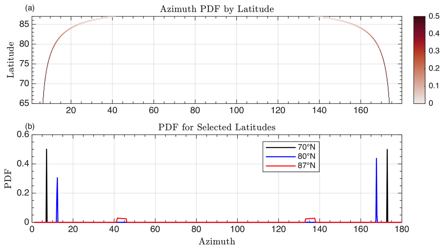
Figure 1 Direction of IS2 transit with respect to a line of longitude (satellite azimuth) as a function of latitude. (a) Probability distribution of azimuthal angle as a function of latitude for all Arctic IS2 RGTs. (b) Probability distribution for latitudes 70° N (black), 80° N (blue), or 87° N (red).

We first identify each optically classified image with its corresponding latitude. The distribution of RGT azimuths (angles with respect to local north) varies as a function of latitude alone and is specified according to the IS2 91 d repeat cycle. Thus at each latitude, we identify the distribution of possible RGT azimuths from the IS2 Technical Specifications (Neumann et al., 2019), with the probability distribution shown in Fig. 1a. We sample from this distribution at each latitude using inverse transform sampling to obtain a distribution of RGT orientations for a Monte Carlo-style emulation of the LIF computation. For most latitudes, the RGT azimuth distribution has approximately only two possible directions (Fig. 1b), though because of the increased track density, the distribution widens approaching the pole (compare the azimuth PDF at 87° N (red) to 70° N (black)).

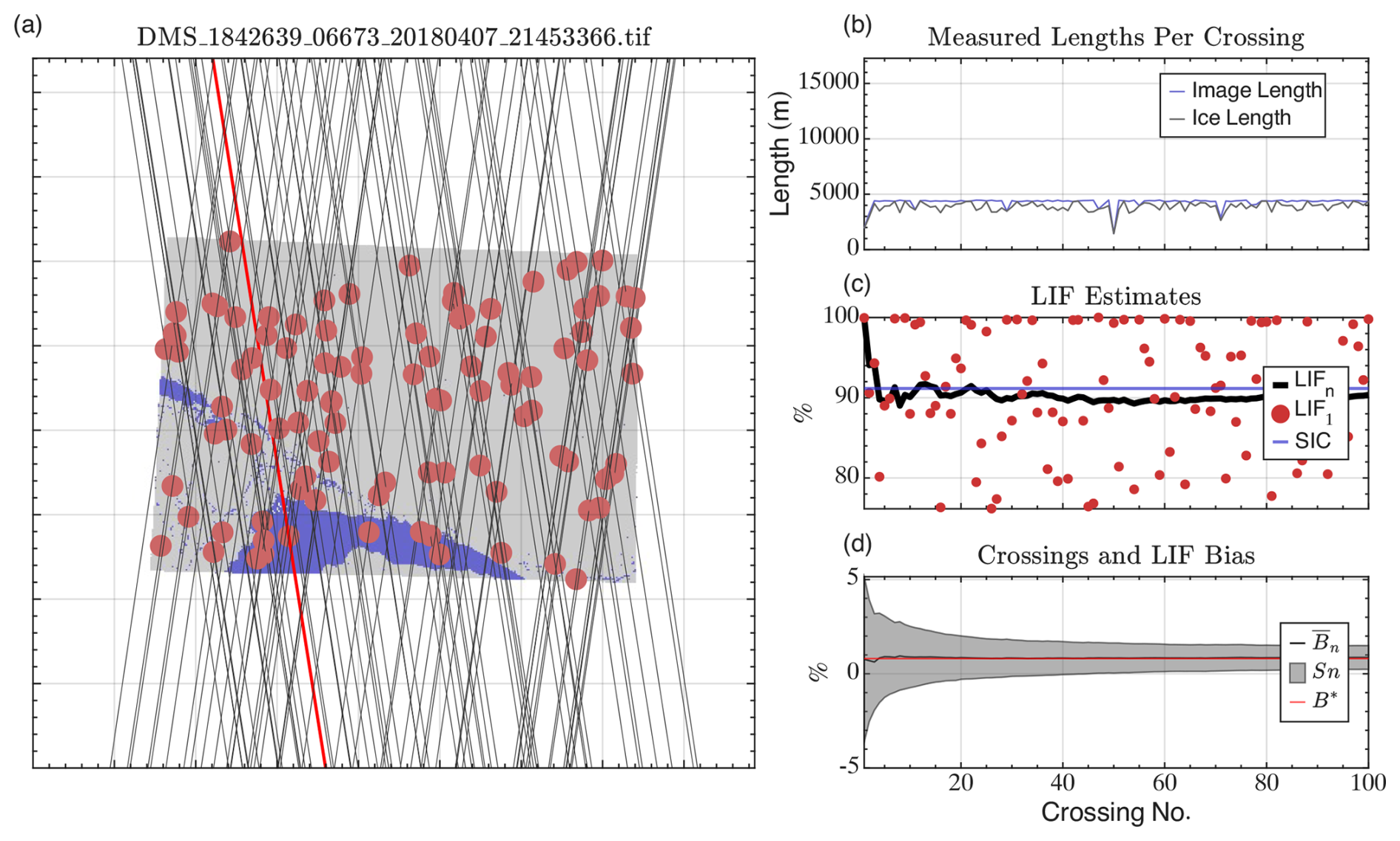
Figure 2 Example application of IS2 emulator to a classified DMS image from OIB. (a) Classified optical image from OIB. Blue points are water, and grey points are ice. Black lines are synthetic IS2 RGTs, which pass through randomly generated tie points (red dots) at the angle distribution appropriate from Fig. 1. The SRGT leading to the most extreme bias is shown as a red line. (b) The total length of all pixels sampled (blue) and the total length of ice pixels sampled (grey) for each SRGT crossing in (a). (c) Single-pass LIF (LIF₁) estimates from each crossing in (b) (red dots), with cumulative LIF_n derived by integrating crossings from (b) in order (solid black line). The true-image SIC is given as a blue horizontal line. (d) The mean (black line) and standard deviation (shaded region) of the LIF_n bias from true SIC (black line), evaluated using all possible permutations of crossings from (a) at cumulative step n. Red line is $B_i^{*}$, the “best-case bias” after sampling all possible crossings. For this image, $B_i^{*}\approx \mathrm{0.8}$ %.

Figure 2 shows the emulation procedure and statistics obtained using the emulator applied to a single image from the optically classified dataset used in Buckley et al. (2025). The particular image shown in the Figure was acquired on 7 April 2018 north of the Beaufort Sea at 75.51° N, 159.3° W and has a sea ice concentration of 92 %. We first take a sample from the appropriate RGT azimuth distribution for this latitude, which at this latitude is approximately 8.75 and −9.1° from due north. For each angle, we then randomly select a corresponding “tie point” in the image (red dots, a) and draw a straight-line crossing through that tie point at the specified orientation angle (black lines). For each such synthetic ground track (SGT_k), we compute the length of ice-covered points, L_I,k, and ice-free points, L_O,k, it intersects and store them as a function of the SGT (Fig. 2b, blue and grey lines). Because the classified imagery is provided on an equal-area grid, we simply count the number of ice and ocean points intersected by the SGT when evaluating the along-track lengths. When applied to real IS2 data (see Eq. 1 and Sect. 3 below), we compute the LIF by weighing ATL07 segments by their length. We repeat this process M=100 times for each image. Each of the M unique SGTs has its corresponding single-crossing LIF, which for image i we term LIF_i,1 (red dots, Fig. 2c). Values of LIF₁ vary significantly given the complex geometry of the scene and distribution of possible tie points and orientation angles. This single-crossing uncertainty for individual images was the subject of analysis for a set of high-resolution images in Buckley et al. (2025). Here for the example image (Fig. 2a), while the mean (across all SGTs) difference between LIF₁ and the true SIC is −1.7 %, the standard deviation is ± 13.55 %. On pass 8 (red line, Fig. 2a), for example, the SGT intersects a large region of open water, recording an LIF₁ of just 75.1 % (not shown in (c)).

The potential high variance in LIF measured from single crossings of the ice surface is uncertainty U2 and necessitates the inclusion of multiple crossings in an ultimate LIF product. To understand the relationship between crossing number and LIF bias, we investigate the convergence of LIF values towards an “optimal” LIF for each image, given its latitude and the preferred orientation of IS2 RGTs. With a set of M SGTs, there are M! different permutations of the set in which the SGTs can be applied. At crossing number n, there are $\left(\genfrac{}{}{0ex}{}{M}{n}\right)=\frac{M\mathrm{!}}{n\mathrm{!}M-n\mathrm{!}}$ unique possible SGT choices from this initial set that could yield an LIF estimate. Given an image, i, crossing number n, and ordered list of SGT indices K, we define the LIF as

$$\begin{array}{}\text{(2)}& {\mathrm{LIF}}_{i,n,K}=\mathrm{100}\times {\displaystyle \frac{\sum _{k\in K}{L}_{I,k}}{\sum _{k\in K}{L}_{I,k}+L_{O,k}}}.\end{array}$$

It is not practical to explore the entire phase space of all possible SGT crossings – instead for each image we select a set of 𝒫 unique sets formed from the SGT list of length M, by sampling with replacement to form sets P_i,k of SGT indices. By sampling with replacement, we form bootstrap estimates of LIF statistics that can be applied in an operational context, when fewer crossings may be available. Without loss of generality, we use the same set of indices for all images (as the individual SGTs are randomly sampled in each image) and drop the i subscript from P, $P_{i,k}=P_k$. Then for each crossing number $n\in [\mathrm{0},M]$, and for each $k\in [\mathrm{1},\mathcal{P}]$, we define the LIF as

$$\begin{array}{}\text{(3)}& \begin{array}{rl}& {\mathrm{LIF}}_{i,n,k}=\mathrm{100}\times {\displaystyle \frac{\sum _{j=\mathrm{1}}^n{L}_{I,P_k\left(j\right)}}{\sum _{j=\mathrm{1}}^n{L}_{I,P_k\left(j\right)}+L_{I,P_k\left(j\right)}}}=\\ & {\displaystyle \frac{\text{length of}\mathit{\text{ice}}\text{points for the first}n\text{crossings in SGT permutation}k}{\text{length of}\mathit{\text{all}}\text{points for the first}n\text{crossings in SGT permutation}k}},\end{array}\end{array}$$

where in this notation P_k(j) is the jth index in the kth SGT list. Each LIF${}_{i,n,P_k}$ is also identified with a bias value:

$$\begin{array}{}\text{(4)}& B_{i,n,k}={\mathrm{LIF}}_{i,n,k}-\mathrm{SIC}.\end{array}$$

With M=100, we select a total number of 𝒫 unique SGT lists, with 𝒫=1000 for each image – and therefore a set of $\left|\mathcal{P}\right|\times M=\mathrm{100}\mathrm{000}$ different estimates of LIF, varying the crossing number and SGT ordering. In total, applied to the 70 225 individually classified images, we have 7 billion emulated LIF calculations. For a given image and crossing number, we use an overbar to denote the average over all SGT replicates (the lists of SGT indices). For example, in image i after n crossings, we define $\stackrel{\mathrm{‾}}{B_{i,n}}={\stackrel{\mathrm{‾}}{B}}_n$ as the mean bias and Si,n the standard deviation of LIF${}_{i,n,k}$ across the 𝒫 replicates. For each image we define the “optimal” LIF, LIF${}_i^{*}$, that is obtained as the bootstrap mean LIF using all M RGTs,

$$\begin{array}{}\text{(5)}& {\mathrm{LIF}}_i^{*}\equiv \stackrel{\mathrm{‾}}{{\mathrm{LIF}}_{i,M,k}}={\stackrel{\mathrm{‾}}{\mathrm{LIF}}}_{i,M}.\end{array}$$

From the “optimal LIF”, we also define the corresponding “optimal bias”,

$$\begin{array}{}\text{(6)}& B_i^{*}\equiv {\mathrm{LIF}}_i^{*}-\mathrm{SIC},\end{array}$$

which has a bootstrap standard error $E_i=S_{i,M}/\sqrt{P}$. We treat $B_i^{*}$ as the “best-case” U2 error, obtained by compiling statistics from the 1000 replicates of 100 crossings of the surface. For the image in Fig. 2, the value of $B_i^{*}$ is 0.8 %, the standard deviation of individual estimates of $B_i^{*}$ is $S_{i,M}=\mathrm{0.6}$ %, and the bootstrap standard error in B^*s is 0.02 %. We examine the statistics of these quantities across all OIB images below and as Fig. 3.

2.2 Bounds on orientation uncertainty as a function of crossing number

Because each replicate is different, the progression from the set of single-crossing LIFs, LIF${}_{i,\mathrm{1},k}$, to LIF${}_{i,\mathrm{1},M}\approx {\mathrm{LIF}}_i^{*}$ is as well. This means that even when the best-case bias $B_i^{*}\sim \mathrm{0}$, there is uncertainty at smaller values of n associated with the variable convergence to the best-case error. For example, when accumulating SGT lengths as ordered in Fig. 2(b), we obtain a sequential list of LIF_n (dropping i and k) values, plotted as a black line in Fig. 2c. The mean absolute bias is less than 2.5 % after four crossings and less than 2.0 % after eight crossings. However the approach to LIF^* differs depending on the replicate, and we can estimate the uncertainty in the estimate of LIF^* by examining the standard deviation across the replicates for each n, S_n. In panel (d) of Fig. 2, we plot both the bootstrap mean bias ${\stackrel{\mathrm{‾}}{B}}_n$ (black line) and the envelope ±S_n (shaded curve). Here we visualize the convergence to S_M=0.6 %. For smaller n there can be substantial variability in S_n: for example it takes five crossings for 2.5 % to lie outside of the interquartile range of B_n,k.

The uncertainty associated with the unknown sampling order declines with increasing n, and for a given image we capture it using the standard deviation among replicates, S_i,n. In a practical application, we will want to know how many intersections would yield an accurate depiction of the SIC, given that we do not know the underlying set of image crossings. This will be represented by the expected value of S_i,n across as many scenes as possible. We take the set of all OIB images and apply the same sampling methodology as detailed above in the example of Fig. 2. This leads to more than 7 billion total replicate LIF${}_{i,n,k}$ and biases $B_{i,n,k}$, which allows us to compute 700 000 sequential estimates of uncertainty in the LIF S_i,n as a function of crossing number, associated with 70 000 best-case-bias estimates $B_i^{*}$. Here we will denote an average across all images using angle brackets – in this notation, $\langle B_i^{*}\rangle =-\mathrm{0.06}$ % is the mean best-case bias across all images. The histogram of best-case biases $B_i^{*}$ is shown as Fig. 3a, which shows the near-zero-mean distribution, as expected given that the orientation between SGTs and sea ice features is random a priori. Best-case biases are generally small, with an interquartile range of (−0.60 %, 0.48 %) (shown as vertical solid black lines in Fig. 3a) and a (5,95) confidence interval of (−2.2 %, 2.1 %) (vertical dashed black lines). The standard deviation of these data is $\langle S_{i,M}\rangle \equiv S^{*}=\mathrm{0.8}$ %, which we will use to represent the fundamental uncertainty in the estimation of SIC with IS2 at a single location, up to 100 image crossings.

As in Fig. 2d (black and red lines), at any crossing number, the bootstrap-mean bias for each individual image approximates the best-case bias for that image: $\stackrel{\mathrm{‾}}{B_{i,n,k}}\equiv {\stackrel{\mathrm{‾}}{B}}_{i,n}\approx B_i^{*}$ for all n. In Fig. 3(b), we show the mean across all images of ${\stackrel{\mathrm{‾}}{B}}_{i,n}$ as a function of crossing number, $\langle \stackrel{\mathrm{‾}}{B_{i,n,k}}\rangle \equiv \langle \stackrel{\mathrm{‾}}{B}{\rangle }_n$ as a black line. As expected, the distribution of this field mirrors $B_i^{*}$ at all crossing numbers and is nearly zero. This demonstrates that, emulated across the set of OIB images, the expected bias from applying the LIF is approximately zero for any crossing number. Thus in a wide application of the LIF to many scenes or many gridded locations, errors in the LIF should approximately cancel out. Still, for accurately estimating LIF in a single area or scene, we note there is significant spread in the bias as a function of crossing number, which results from the variability in sampling for each crossing. In Fig. 3b, therefore, we shade the expected uncertainty as a function of crossing number, $\langle S_{i,n}\rangle \equiv \langle S{\rangle }_n$. Given the near-zero expected bias $\langle \stackrel{\mathrm{‾}}{B}{\rangle }_n$, 〈S〉_n is also the expected error in SIC at crossing n. Whereas $\langle \stackrel{\mathrm{‾}}{B}{\rangle }_n$ quantifies the expected bias for a typical scene, 〈S〉_n quantifies the uncertainty in the bias estimate for that particular scene. For a single crossing, we see that $\langle S_{i,\mathrm{1}}\rangle =\mathrm{9.02}$ % – which, while lower than the single-crossing uncertainty from the example image in Fig. 2, is still significant. This uncertainty declines with increasing n. From the analysis of Buckley et al. (2025), we found that a typical overestimation of SIC from PM products compared to the OIB data was 2.5 %. Thus we are interested in the number of crossings so that uncertainty in the typical LIF measurement is less than this. In Fig. 3b, as a solid line we show the first value of n, which we call n^*, with 〈S〉_n<2.5 %. This occurs when $n^{*}=\mathrm{11}$ crossings. While at $n^{*}=\mathrm{11}$, 〈S〉_n<2.5 %, the distribution of $S_{i,n^{*}}$ is non-uniform. We show the histogram of $S_{i,n^{*}}$ as Fig. 3c, along with the interquartile range and (5,95) intervals. The uncertainty in the bias for any scene is positive–definite, 75 % (95 %) of all $S_{i,n^{*}}$ values less than 3.63 % (6.35 %).

To summarize our findings, we implemented an emulation system to draw accurately oriented IS2 “crossings” over 70 000 segmented images from OIB. We find that there is no systematic bias in LIF associated with the orientation of tracks, i.e., $\langle B{\rangle }_n\sim \langle B^{*}\rangle \approx \mathrm{0}$. While this implies that many separate measurements of LIF will have an average bias near zero, this is not true for individual scenes. The error in approximating SIC for a given scene declines with crossing number, and after 11 crossings we find that the uncertainty in estimating the SIC, $\langle S_{i,n^{*}}\rangle$, is less than 2.5 %. The distribution of actual errors after 11 crossings has a long tail, but 95 % will have a bias below 6.35 %. Below, when developing a gridded LIF product, we will ensure that any grid cell where LIF is reported and compared to PM SIC has at least this many crossings.

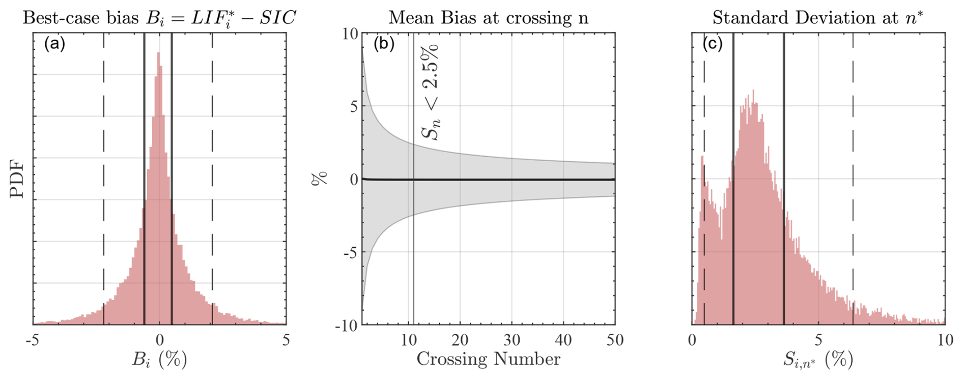
Figure 3 Statistics of bias and uncertainty associated with LIF when using data from all 70 225 classified OIB images. (a) Histogram of best-case bias in SIC, $B_i={\mathrm{LIF}}_i^{*}-\mathrm{SIC}$. Vertical lines are interquartile range (solid, −0.60 % to 0.49 %) and (5,95) interval (dashed, −2.23 % to 2.10 %). (b) Cross-image average of bootstrap-averaged bias (black line) as a function of intersection number, $\langle \stackrel{\mathrm{‾}}{B}{\rangle }_n$. Shaded region encompasses cross-image-average of bootstrap-averaged standard deviation 〈S〉_n. Vertical line shows the crossing number, $n^{*}=\mathrm{11}$, after which 〈S〉_n is less than 2.5 %. (c) Histogram of $S_{i,n^{*}}$ at crossing number n^*. Vertical lines are interquartile range (solid, 1.64 % to 3.63 %) and (5,95) interval (dashed, 0.49 % to 6.35 %).

3 A Global ICESat-2-based linear ice fraction product

Leveraging the uncertainty information obtained through emulation, we next seek to build an SIC product built from the IS2 LIF. As the data evaluation of Buckley et al. (2025) focused on Arctic scenes, we will focus on Arctic data only – though we do provide Antarctic LIF data in Horvat (2024a). These data and code for generating a global gridded product of LIF-based SIC are provided through the MATLAB-based package IS2-Grid version 0.4 (Horvat, 2024a). This software package is designed to produce modular gridded sea-ice-related products at requested temporal and spatial gridding through an accumulation of multiple tracks, for comparison with climate model and observational data. It permits the rapid development of cumulative statistics over chosen temporal windows and currently provides estimates of the floe size distribution, significant wave height, and sequential LIF along with other ancillary statistics. This code is modular and provides a simple way for creating gridded products from along-track-calculated statistics. Here we use that code to generate an LIF product on a monthly timescale on the 25 km Arctic polar stereographic grid.

This monthly 25 km LIF dataset is evaluated against six widely used PM-SIC products. Four rely on brightness temperatures from the Special Sensor Microwave – Imager/Sounders (SSMI/S) on board US Defense Meteorological Satellite Program flight units 16–18. They are (1) the NASATeam (NT) (Cavalieri et al., 1984) algorithm; (2) the Bootstrap (BT) algorithm (Comiso and Sullivan, 1986); (3) the NSIDC Climate Data Record (CDR), equal to the maximum of the Bootstrap and NASATeam algorithms (Meier et al., 2014); and (4) the OSISAF Global Sea Ice Concentration climate data record (OSI450-a, up to 31 December 2020) and interim climate data record (OSI430-a, up to 2023) (Lavergne et al., 2019a). We also include two algorithms using brightness temperature data from the Advanced Microwave Scanning Radiometer 2 (AMSR2) sensor on board the JAXA GCOM-W satellite, computed using (5) the NASAteam2 algorithm (Meier, 2018) and (6) the ASI-ARTIST algorithm (Spreen et al., 2008). Products (1)–(3) and (5) are provided on the NSIDC 25 km polar stereographic grid. We use OSI450/430 products (4) on the 25 km EASE grid and (6) the ASI-ARTIST product on a 6.25 km polar stereographic grid, both of which we regrid to the NSIDC 25 km polar stereographic grid. We analyze PM-SIC and IS2 data across the time period from the launch of the IS2 satellite in October 2018 until December 2023 for 63 months including 5 full calendar years. Further details on the PM-SIC algorithms and satellite platforms used can be found in Buckley et al. (2025).

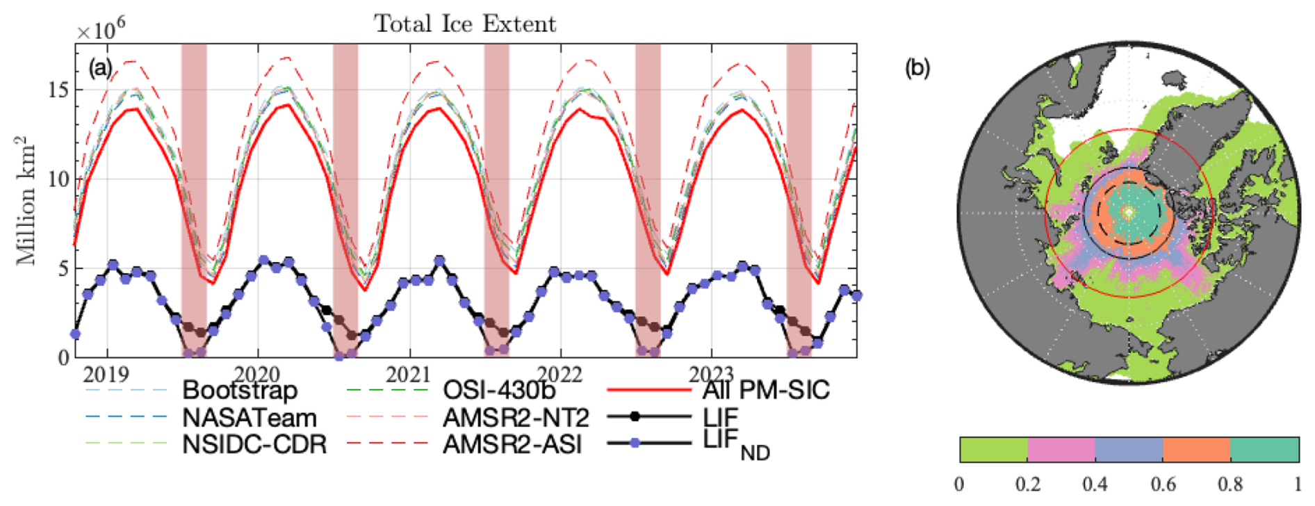
Figure 4 Comparison of coverage of IS2 LIF data to commonly used PM-SIC products. (a) Arctic sea ice extent of 6 PM-SIC products (dashed colored lines) compared to the area well-sampled by IS2 (black line, black scatter) from October 2018–December 2023. Black line with blue scatter is the IS2 extent when excluding areas with more than 2.5 % dark lead fraction, LIF_ND. “Summer months” have red background. (b) Percentage of months from October 2018–December 2023 where PM-SIC record sea ice and IS2 tracks are sufficiently dense. Red latitude circle shows average latitude of grid cells which have 15 % or more SIC in all PM products. Black latitude circle shows average latitude of LIF extent. Dashed black circle shows average latitude of LIF extent in summer months.

3.1 Uncertainty in temporal sampling from IS2

In addition to the uncertainties with orientation and surface classification, when building a longer-timescale product, we must consider that IS2 overflights exhibit temporal intermittency compared to PM measurements that are retrieved daily. At each grid point, we define an “IS2 intermittent” PM SIC, $\stackrel{\mathrm{̃}}{c}$, equal to the segment-averaged PM sea ice concentration using the along-track-defined PM SIC. Two reference PM datasets are included along track with the IS2 ATL07 product, the NSIDC CDR (all ATL07 versions) and the AMSR2-NT2 product (ATL06 v6 and later), and we use both for this purpose. We define the “temporal intermittency bias”, B_T, from a monthly average SIC, $\stackrel{\mathrm{‾}}{c}$, as

$$\begin{array}{}\text{(7)}& B_{\mathrm{T}}=\stackrel{\mathrm{̃}}{c}-\stackrel{\mathrm{‾}}{c}.\end{array}$$

The value of B_T measures how different the monthly PM-SIC product would be if it included only data from the days when IS2 flew overhead. Thus it estimates a potential bias in SIC introduced by IS2's intermittent temporal sampling. As we do not want to consider this additional uncertainty, we ignore any grid cell where $\Vert B_{\mathrm{T}}\Vert$ exceeds 2.5 % in either of the AMSR2-NT2 or NSIDC-CDR products. This reduces the number of grid cells over which we develop an LIF product. We combine this restriction with the requirement that the grid cell was intersected by at least 11 separate IS2 beam crossings. We also require that all PM-SIC estimates have greater than 15 % SIC at any location, eliminating any potential dependency of intercompared LIF data on the PM-SIC 15 % cutoff used to define ATL07. In Fig. 4a, we plot sea ice extent for all PM products (dashed lines), equal to the sum of grid areas where local PM SIC exceeds 15 %. We use the quality control restrictions to define two further sea ice extents. The first is the “comparable” sea ice extent, which is the sum of all grid areas where each local PM-SIC value exceeds 15 %. In Fig. 4 this is plotted as a solid black line. We show the “LIF extent” as the comparable sea ice extent with at least 11 IS2 beam crossings as a solid black line. Comparable sea ice extent ranges from 3.7 and 14.1×10⁶ km². The LIF extent is smaller, ranging from 0.9 to 5.5×10⁶ km². As a percentage of the comparable sea ice extent, this is between 21 % and 46 % of the total. For comparison, if we do not impose a restriction on $\Vert B_{\mathrm{T}}\Vert$, the LIF extent ranges from 1.8 to 5.8×10⁶ km² (from 21 % to 62 % of comparable sea ice extent), with the most significant impact in summer months.

Because of the higher track density near the pole, areas that make up the LIF extent are typically at high latitudes and have correspondingly high SIC. In Fig. 4b, we plot the fraction of all months when a grid cell both is “comparable” (with sufficient SIC as recorded by PM algorithms) and has enough IS2 crossings to be compared. For regions above 80° N, this is nearly all months. Whereas the average latitude of the comparable sea ice points is 75.1° N, denoted by a solid red line of latitude in Fig. 4b, it is 82.0° N for points within the LIF extent, which is denoted by a solid black line of latitude and is significantly more poleward. The densest coverage of IS2 is at these high latitudes, in areas of compact sea ice with leads. This makes LIF particularly appropriate for comparison with PM SIC, given the focus of Buckley et al. (2025) on the overestimation of SIC by PM in these sea ice regions.

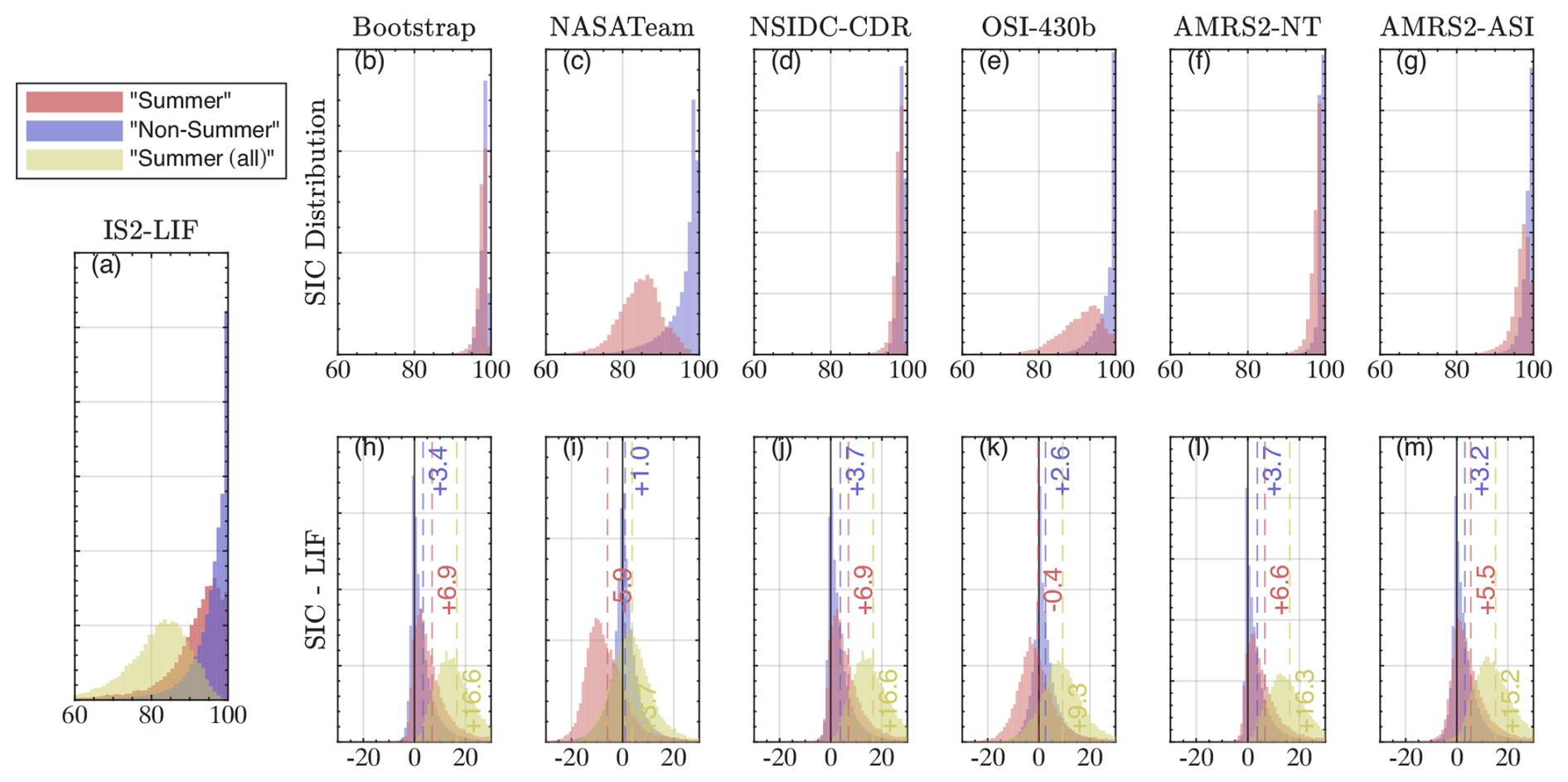
Figure 5 (a) Histogram of IS2-LIF, using specular returns only in “summer” (July and August, red) and non-summer months (blue). Gold shows LIF distribution in summer months when including dark leads. Top row: (b–g) same as (a) for the six PM-SIC products. Bottom row: (h–m)) difference from PM-SIC products and the three LIF products in (a). Summary statistics are provided in Table 1. Vertical lines and labels are mean Δ values between PM SIC and the corresponding LIF product.

3.2 Comparison of gridded LIF data with passive microwave products

Figure 5 shows histograms of SIC values (top row, b–g), and the differences from LIF, Δ (bottom row, h–m) for all data, for each PM-SIC product. Figure S1 shows the distribution of LIF values in each month for two LIF products. Qualitatively and quantitatively, when including all dark leads as open water (see below), the LIF distribution is different in the months of July and August from the rest of the year, which is also the case for some PM-SIC products. Including dark leads in those months leads to a median LIF of 82 % and 84 %, compared to above 92 % in all other months. July and August are also where melt ponding is significant at the high latitudes we consider here (Istomina et al., 2025). To differentiate between these potentially melt-affected results, we segment the LIF data into “summer” or pond-affected months covering July and August (Fig. 5 red and gold) and “non-summer” data covering September to June (Fig. 5, blue). The months of June, September, and October also are distinct from the other non-summer months in that the modal LIF is not 100 %. While there are distinct histograms of PM SIC and LIF during these months (see Table 1), they have significantly higher LIF than in July and August, and the overall results of this study are not materially affected by their inclusion as “non-summer” months.

3.3 Dark vs. specular leads in LIF retrievals

The IS2 surface type field includes two radiometrically derived classification for open-water points: “specular” or “dark” leads. Each could potentially be considered open-water segments in this work. Leads in ICESat-2 are identified where the ATL07 segment has a high photon rate, a narrow photon distribution, and Lambertian surface characteristics as determined by the ratio of the photon rate to the background photon rate normalized by the sun elevation. Dark leads are identified as the leads with the lowest photon rate. These “dark leads” can be at least partially contaminated with both open water and cloudy returns (Saha et al., 2024) and are responsible for a significant difference between summer and non-summer LIF data due to known issues in classifying surface meltwater in both PM and IS2 products (Kwok et al., 2019b; Tilling et al., 2020; Farrell et al., 2020; Herzfeld et al., 2023). In Fig. 5, we plot histograms in summer months that include (gold) or exclude (blue) dark lead segments as open water. We show histograms of the difference in the LIF between the two as Fig. S2 in the Supplement as a function of month. We additionally show in Fig. 6a the difference between LIF_spec and LIF using all dark leads as open water in summer and non-summer months. As seen in Fig. S2, the inclusion of dark lead classifications plays an important role only in July and August but not in other months. The impact of dark lead segments on the overall LIF distribution can be seen in Fig. 5, where the shape of the LIF histogram including all dark leads in summer months (gold histogram) peaks at 81 %, with no areas of 100 % LIF. On average, including dark leads as open water leads to a reduction in LIF by 9.7 % in July and August. By contrast, the specular LIF (blue) is significantly closer to 100 % and more closely resembles both the non-summer LIF values (blue) and those derived from PM algorithms (top row), up to the biases seen in non-summer months. Outside of July and August, the net impact of including dark leads in the LIF calculation is very small as there are few dark leads contributing a mean difference in LIF of 0.4 % (Fig. 6a, blue histogram).

The peaked distribution of LIF including dark leads contrasts with the histogram of LIF values in all other months (see “non-summer” months in Figs. 5 and S1 and S2), where the histogram of LIF values increases monotonically as LIF increases. As the characteristic response of leads likely does not change season to season, this points to a potential role of sea ice surface melt in altering the surface returns and possible misidentification of “dark lead” segments. Investigations of summer sea ice melt have shown melt ponds identified as both dark and specular leads (Farrell et al., 2020), and the melting snow/slush layer may also be misclassified as leads. Summer Δ values (right columns, Table 1, and vertical lines, Fig. 5h–m) are typically large and positive when including these dark lead segments. Two PM-SIC products also show a peaked distribution of SIC values in July and August, the NASATeam and OSI-430 algorithms, which both are implemented on the SSMI/S sensor platform. The OSI-430 algorithm (Lavergne et al., 2019a) is tuned to represent the NASATeam algorithm for high SIC values (Lavergne et al., 2019b; see Sect. 3.2.4) and therefore may also reflect similar biases in the Comiso and Sullivan (1986) algorithm. Analysis of NASATeam-based SIC data in Arctic summer has shown these months to have both enhanced variability and enhanced uncertainty (Brucker et al., 2014) related to melt ponding. For the summer comparisons, the mean latitude of comparable LIF data is 84.5° N (dashed line, Fig. 4). For each calendar month, as in Fig. S4, we show the fraction of the period when IS2 is operational and where we find sufficient IS2 crossings to produce the LIF product. In most months this is highly restricted to the highest latitudes, especially in summer months. Sea ice in this region is typically compact. Given the known uncertainty in both lead detection and PM-SIC retrievals from the NASATeam over ponded sea ice, this dually suggests that the low mean SIC and LIF values during these months may be due to errors induced by surface melting.

Because of the potential errors associated with dark lead classification, the similarity in SIC histograms with other PM-SIC products that are known to be biased or more uncertainty in summer months, and the minimal impact of dark leads outside of months with surface melting, here we provide the product that includes only “specular” leads as open water in all months as the core LIF product, which we denote LIF_spec. In the comparisons that follow, we also generate a LIF product which masks any grid cells where the dark lead fraction greater than 2.5 %, which we term LIF_ND. The coverage of this reduced dataset is plotted as a dashed black line with blue scatter in Fig. 4a. Eliminating areas with high dark lead fraction reduces LIF coverage by 85 % in summer but just 3 % outside of the melt season and in total reduces LIF extent by 18 % by significantly limiting summer intercomparisons.

Some dark lead segments are appropriately classified as open water (Petty et al., 2021; Koo et al., 2023; Liu et al., 2025; Buckley et al., 2025), and therefore LIF may be reduced by up to 0.4 % outside of the melt season or 9.7 % in summer depending on what fraction of these dark leads are truly non-sea-ice points. As discussed as uncertainty U1 (classification uncertainty), some areas of open water may be inappropriately classified as sea ice. Improved classification of IS2 segments, including by adding additional radiometric features and machine learning (e.g., Liu et al., 2025), can lead to enhanced confidence in LIF, especially in summer months. We repeat Fig. 5 using LIF_ND as Fig. S3 but find this does not materially affect the qualitative and quantitative analysis of biases between LIF and PM-SIC products that follows. We focus our analysis on LIF_spec alone but discuss the implication and use of LIF_ND in Sect. 4.

Statistics derived from the distributions shown in Fig. 4 is given in Table 1, along with interquartile ranges and mean differences from LIF, $\stackrel{\mathrm{‾}}{\mathrm{\Delta }}$. There are approximately 25 000 “summer” comparison points, covering 17×10⁶ km², and 278 000 “non-summer” comparison points, covering 182×10⁶ km² – larger because of the larger spatial extent of sea ice and greater number of months included. The sea ice areas being intercompared here are highly compact – with a mean SIC for NSIDC-CDR of 98 % in summer and 99 % non-summer months, reflecting a similar sea ice regime, as was examined in Buckley et al. (2025), and the possibility of overestimation of SIC in both seasons. All PM-SIC products indicate a higher ice fraction than the LIF in all seasons. Non-summer biases are similar to that found in OIB data as well as in classified optical data, with a median positive difference of 0.5 %–2.1 % for sea ice that was recorded by LIF as being 94.3 % ice-covered on average and 98.2 % on average for the NSIDC-CDR PM-SIC product.

Table 1 Comparison of “summer” (July and August) and “non-summer” (all other months) statistics of IS2 global LIF product and related products and the set of six examined PM-SIC products. Δ values are differences from standard LIF product, which includes only specular leads in summer and all leads in non-summer months. Values in parentheses next to strong/weak beam LIF products indicate fraction of LIF extent with sufficient data. $\stackrel{\mathrm{‾}}{\mathrm{\Delta }}$ is the mean difference from the LIF product LIF_spec. Values in parentheses show the interquartile range of Δs (25 %–75 % intervals). Percentages for LIF products are the fractions of total LIF coverage for each product.

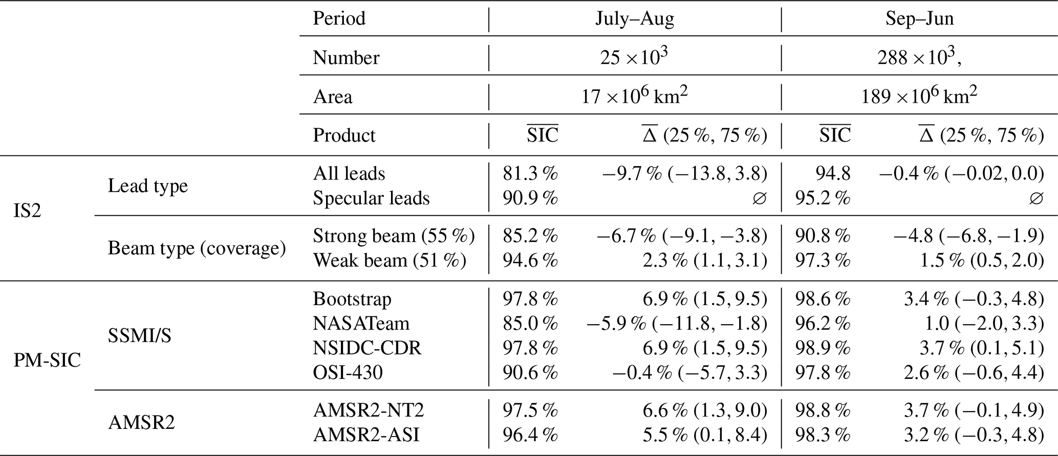
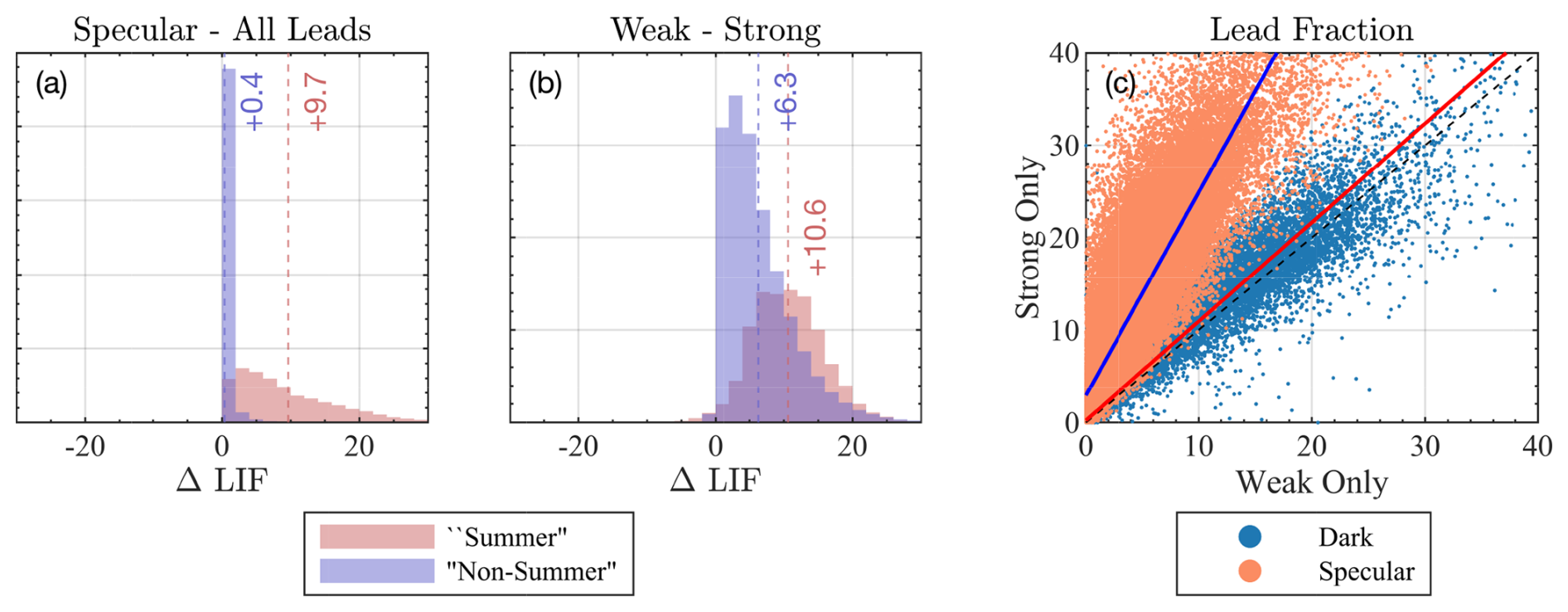
Figure 6 (a) Histogram in “summer” (July–August, red) and “non-summer” (September–June, blue) months showing the difference between LIF evaluated using specular returns only (LIF_spec) and including dark leads as open water. (b) Same but for the LIF calculated using only weak beams minus using only strong beams. Calculations for (a) are taken over the entire LIF extent. Calculations for (b) are taken over the area where there are at least 11 separate strong beam and weak beam crossings, which is approximately 50 % of the LIF extent. (c) Comparison of dark (blue) or specular (orange) lead fraction for strong beams only (y axis) or weak beams only (x axis). Dashed black line is 1 : 1 line. Solid red lines are linear fits to each respective set of data for all points with nonzero lead fraction.

3.4 Strong vs. weak beam retrievals

IS2 has six separate beams, of which the three strong beams have 4 times the energy of the weak beam and consequently 4 times the photon return and approximately 4 times the along-track resolution (Markus et al., 2017). The difference in beam energy leads to differences in the classifications of lead segments. We compute summary statistics of LIF data evaluated using strong and weak beams alone in Table 1. To determine the LIF using just a single beam strength, we apply the same quality control on the reduced subset of IS2 crossings: for example we require at least 11 strong beam crossings to produce an LIF product in a given month and location. Doing so restricts the area over which such products can be compared, with the strong beam coverage just 55 % of the overall LIF extent and the weak beam coverage just 51 %. In these areas, we see significant biases between each and the overall LIF product, which blends the two. From September–June, the strong beam has an offset of −4.8 % from LIF_spec, whereas the weak beam has a positive offset of 1.5 %. In this period, months, weak-only LIF reports an SIC of 97.3 %, which is similar in magnitude to that from the PM-SIC products, whereas the strong-only LIF is significantly lower.

Since LIF_spec can include both weak and strong beams to reach 11 crossings, to additionally compare a strong-only and weak-only LIF product, we examine only those areas where there are both 11 weak beam crossings and 11 strong beam crossings. In those areas, we plot the summer and non-summer histograms of LIF calculated using just weak beams and just strong beams as Fig. 6b. Overall, this is an area covering 50 % of the LIF extent. In this area, weak-beam-only LIF is on average 10.6 % higher than strong-beam-only LIF from July–August and 6.3 % higher from September–June. In non-summer months the modal weak-strong offset is near 0 %, but there is a peak in July and August around the mean offset of 6.3 %.

The difference between strong and weak beams is caused by an increased fraction of specular lead classifications by the strong beam. The specular lead classification requires a higher photon rate compared to the dark lead classification and thus is more common in the beams with higher energy. In Fig. 6c we scatter dark (blue) and specular (orange) lead fraction for the strong-only (y axis) or weak-only (blue axis) LIF data. As in (b), these data are presented only for grid areas where there are more than 11 strong and more than 11 weak beam crossings, a total of 157 000 distinct measurements points. For those points, there is a high correlation (r²=0.97) between the dark lead fraction in the two datasets, with the best linear fit (red line, slope 1.06) nearly 1–1 (dashed black line). In contrast, there is still a weaker correlation between respective specular lead fractions (r²=0.89), and the best linear fit is closer to 2–1 (blue line, slope 2.18). Out of the 157 000 points, 133 000 (85 %) have nonzero dark and specular lead fractions in both strong and weak products. Of these, the median strong beam LIF measurement has a specular lead fraction 5.3 % higher than its corresponding weak beam LIF, but the median dark lead fraction difference is just 0.06 %.

4 Conclusions

In this study, we developed a new gridded data product from the IS2 laser altimeter, the LIF. We evaluated errors in the representation of the sea ice surface using an emulator which is run on a set of classified optical images from NASA's OIB. We showed that, in general, PM-SIC measurements were positively biased against IS2 estimates, particularly in non-summer months, as was the case when compared to imagery in Buckley et al. (2025) and in the previous literature (e.g., Kern et al., 2019). IS2 is particularly effective at estimating SIC, even with a limited number of beam crossings, especially in regions of compact sea ice with leads. With further validation of the ATL07 surface classification scheme, this product may help reduce open-water biases significantly.

The IS2-LIF product is provided as a global, monthly product covering 21 %–46 % of the Arctic sea ice zone. This data product is available through December 2024 (see “Code and data availability”). Because of the available comparative data from OIB, we only included Arctic comparisons in this work, though the data product has been made available in both hemispheres. In months from September–June (“non-summer”), we found that the offset between LIF data and PM-SIC product data was of the same order of the bias between the OIB optically classified imagery and PM-SIC data we found in Buckley et al. (2025). Because of this consistency, we suggest that this captures an overestimation bias in the PM-SIC products, and this offset is not from misclassification error in the ATL07 product. In periods of the year associated with surface melting (here, July and August, when high-latitude sea ice is experiencing peak melt), we found that high levels of possible misclassification of surface water in the form of “dark leads” can degrade the quality of the LIF product in similar ways to PM-SIC products. Because the impact of dark lead classifications on LIF is only significant in these months, we suggest the use of only specular leads for calculating LIF, especially in months where there is the potential for surface melting. Because of the ambiguity in dark leads, we also examined a product which eliminated grid cells with an appreciable dark lead fraction, LIF_ND. This leads to a substantial reduction in LIF extent in summer months but little change in non-summer months. Overall, non-summer month statistics are similar compared to LIF_spec (see Fig. S3), with larger positive offsets in the PM data in summer. In general, because of the association of dark leads with surface melting and errors in classification, we advise excluding dark leads from the analysis by using the “specular” LIF product LIF_spec.

In examining differences between IS2's weak and strong beams, we found that the classification of “dark” leads by weak and strong beams was nearly identical as a portion of overall sea ice segment length but that specular leads were approximately twice as common in strong beam samples than weak beam samples, similar to findings in Petty et al. (2021). This leads to consistent weak–strong LIF differences of up to 10 % in summer months. Since weak and strong beams are sampling approximately the same sea ice, the difference is likely a consequence of differences in the processing of sea ice surface returns between the two products. The weak-only LIF product aligns with estimates of SIC from PM-SIC products, but with a power and resolution one-quarter that of the strong beams, it is possible that openings in the sea ice cover are missed or averaged over that are captured by the strong beam. In other studies, weak beam data can be degraded relative to strong beam data when evaluating variable along-track statistics (Zhu et al., 2020), with strong beam measurements of higher quality for reconstructing surface types from classified imagery (Liu et al., 2025). Future work aimed at understanding weak–strong differences in collocated imagery will be important in understanding whether weak beam returns should be disregarded or strong beam retrievals overestimate the fraction of open water along track or a combination of both.

While we have constrained the errors in LIF arising from uncertain temporal and spatial sampling through emulation, there is significant room to improve the LIF product through surface-type classification. This comes about in two ways: first by improving the classification of “dark lead” segments in summer and second by constraining the differences between weak and strong beam reconstructions of the surface. Typical summer dark lead fractions are 9.7 %, and whether this represents melt ponding, surface melt, or open water can be further constrained. The variable inclusion of weak or strong beams alters LIF significantly in all months, due to an approximate doubling of specular leads in the strong beams relative to the weak beams. Both weak-only and strong-only products show an overestimation of SIC by PM products, but the degree and importance of this overestimation should be further understood and rectified by assessing which of the two accurately depicts the sea ice surface.

The evaluation of LIF in representing local SIC primarily focused on areas of compact sea ice in Buckley et al. (2025), and because of the preprocessing steps employed in generating the monthly LIF product, nearly all locations of intercomparison in Sect. 3 were also compact ice. For example, as indicated in Table 1, mean NSIDC-CDR in the intercompared regions for producing Fig. 5 exceeds 98 % – just 0.07 % of points had an NSIDC-CDR less than 80 %. This limits the degree to which the 15 % NSIDC-CDR mask used to define the ATL07 can influence LIF data. The LIF product has not yet been validated for low-concentration ice or the CDR-defined marginal ice zones, and its utility in those regions remains an open question, although these areas are critical for understanding overall sea ice variability (Bennetts et al., 2022; Squire, 2022; Horvat, 2022). The LIF product therefore may provide an independent and possibly improved estimate of SIC in high-concentration, non-melt-affected months, though it has not been examined in areas where the sea ice has a low concentration or is highly variable.

In general, evaluating LIF_spec including both weak and strong beam crossings, we find a positively skewed distribution of July–August SIC values in all PM-SIC products except the NASATeam and OSI-430. As discussed, these two PM-SIC products may be overly sensitive to surface melting. Other products all report compact sea ice and distributions of SIC that resemble non-summer months, with positive biases of 5.5 % to 6.9 %. For example, compared to the NSIDC-CDR, LIF_spec suggests there is more than 400 % more open water in these months. In non-summer months, we see overestimation biases in all PM-SIC products, with from 1.0 % (NASATeam) to 3.7 % (NSIDC-CDR) more SIC in the PM products, which varies depending on whether weak beam data are included or excluded. Again, compared to the NSIDC-CDR, LIF_spec suggests there is more than 400 % more open water in compact ice zones at high latitudes in the non-summer months. These overestimations match in magnitude with the comparisons between IS2 and PM-SIC data as well as comparisons between PM-SIC and optically classified OIB data in Buckley et al. (2025) as well as other intercomparisons (Ivanova et al., 2015; Kern et al., 2019).

As it illuminates biases, particularly in compact sea ice in non-summer months, LIF derived from IS2 offers an opportunity to enhance estimates of sea ice concentration. Underestimations of SIC outside of the melt season may not be large, but these differences correspond to large increases in open water fraction, which can drive ocean and atmospheric variability. Climate models that are tuned to reproduce sea ice anomalies from PM satellites, or that assimilate PM SIC for forecasts, may underestimate the magnitude of this air–sea exchange. We used validation data from high-resolution optical imagery and an emulation tool. It will be necessary to enrich this LIF data with more constraints to ascertain the year-round and repeat skill of LIF and its potential for developing a new SIC data product on shorter timescales. IS2 offers a high-resolution and repeatable opportunity to provide improved PM-SIC measurements and greater understanding of overall sea ice variability in the polar seas.