Improved permafrost modelling in mountain environments by including air convection in a hydrological model

Permafrost occurrence in mountainous regions is influenced by complex topography and surficial geology, leading to high spatial heterogeneity. Coarse sediments create a unique thermal regime that allows permafrost to persist even under positive mean annual air temperatures due to natural convection lowering ground temperatures. Although this process has been recognized as a key factor in explaining the persistence of permafrost formation within coarse sediments, studies assessing the impact of natural convection on ground temperatures and permafrost are limited, partly due to the absence of hydrological models that take this process into account. This article expands on a well-established hydrological model to incorporate the effects of natural air convection on heat transfer. The modified model includes airflow through Darcy's equation and the Oberbeck–Boussinesq approximation to account for density-driven buoyancy effects, as well as a heat advection–conduction equation for the air phase without assuming local thermal equilibrium between the air and the other phases. The model was tested on a talus slope in the Canadian Rockies, where conventional models failed to represent field-based evidence of permafrost. The results revealed that coarse-sized sediments can lower ground temperatures by several degrees when natural convection is considered. Additionally, the study demonstrated that local thermal equilibrium approaches underestimate the impact of natural convection especially on short timescales. This enhanced model improves our understanding of permafrost dynamics in alpine landforms and enables a more accurate analysis of permafrost extent and its influence on groundwater discharges.

1 Introduction

Mountains play a fundamental role in providing water resources for the environment and society, with nearly 40 % of the global population relying on mountain runoff (Viviroli et al., 2020). These environments possess unique hydrological characteristics, sustaining streams throughout the year through diverse water storage processes – groundwater, lakes, snow, glaciers, and permafrost – collectively supplying water across broad timescales (Jones et al., 2019). Within mountains, particular landforms like talus slopes, moraines, and rock glaciers stand out as key hydrological and ecological components of high-altitude basins. Recent field-based studies have shown that water released from these landforms contributes a relatively large fraction of the annual streamflow despite covering a relatively small area (Chen et al., 2018; Harrington et al., 2018; Hayashi, 2020; Somers et al., 2016; Winkler et al., 2016). Additionally, mountainous landforms exhibit unique thermal characteristics, where the presence of coarse sediments creates a distinctive ground thermal regime, establishing them as cold-condition strongholds since their persistently cold discharges are critical for the ecological balance of mountain ecosystems (Brighenti et al., 2021; Harrington et al., 2017; Morard et al., 2008). Permafrost, defined as the subsurface material with temperatures below 0 °C for at least 2 consecutive years (van Everdingen, 1998), is likely to occur within these landforms, even under positive mean annual air temperature (MAAT) (Wicky and Hauck, 2017; Delaloye and Lambiel, 2005; Haeberli et al., 2011; Gorbunov et al., 2004; Bächler, 1930; Hoelzle, 1992). This context underscores the importance of understanding the thermal processes occurring in mountainous landforms as a necessary step to characterize the influence of permafrost in the hydrological balance of mountain environments.

The presence of permafrost directly influences subsurface water flow. As soil reaches freezing temperatures, water becomes ice, hindering or blocking flow depending on the ice content. Permafrost generally acts as a confining layer, creating two main flow paths: near-surface flow above the permafrost (supra-permafrost) and deeper subsurface flow (sub-permafrost) (Giardino et al., 1992; Woo et al., 1994; Langston et al., 2011; Harrington et al., 2018). However, when permafrost is discontinuous or contains low ice content, intra-permafrost flow may also occur. Regarding the contribution of ice melt to streamflow, several studies have shown it is not highly significant in alpine landforms (Krainer and Mostler, 2002; Arenson and Jakob, 2010; Harrington et al., 2018; Hayashi, 2020). Thus, the primary function of permafrost in alpine hydrogeology is to control the subsurface water flow paths.

A relevant factor controlling permafrost occurrence in mountainous landforms is the presence of coarse, blocky sediments. Studies have shown that coarse sediments can sustain lower temperatures than adjacent fine-grained soils, primarily due to the combined influence of density-driven air convection and lower thermal conductivity (Gorbunov et al., 2004; Haeberli et al., 2011; Gruber and Hoelzle, 2008). Abnormally low ground temperatures at relatively low elevations, often indicative of isolated permafrost patches, have long been documented in porous debris accumulations such as talus slopes and, in some cases, relict rock glaciers (Wakonigg, 1996; Morard et al., 2010; Sawada et al., 2003). During winter, large temperature gradients between the ground and the air can promote air convection inside high-permeability deposits, resulting in a strong coupling of the heat transfer processes between the atmosphere and the subsurface (e.g. Juliussen and Humlum, 2008; Pruessner et al., 2018). One example of this effect can be seen in landforms with steep slopes, such as talus slopes, where non-vertical air convection occurs during winter and summer, generating a thermal anomaly. While, in general, air and ground surface temperatures decrease with elevation (Rolland, 2003), internal air convection can override this relationship and lead to colder conditions on the lower part of a talus slope (e.g. Morard et al., 2008; Delaloye and Lambiel, 2005; Wagner et al., 2019; Wicky and Hauck, 2017; Wiegand and Kneisel, 2024). In addition, the coarse sediments' low thermal conductivity influences the seasonality of heat transfer, contributing to an overall decrease in ground temperatures (Gruber and Hoelzle, 2008). The heterogeneous nature of snow cover over these complex, non-smooth surfaces further influences heat transfer processes in coarse sediments, reducing the snow insulation effect (Haeberli et al., 2011).

Various numerical models have been developed to examine the complex interplay of processes influencing permafrost occurrence (Grenier et al., 2018). They have contributed to understanding the influence of groundwater flow in permafrost environments by coupling the flow and heat transport equations, including dynamic freeze–thaw processes. For example, SUTRA-ICE (McKenzie et al., 2007) and PFLOTRAN-ICE (Karra et al., 2014) are comprehensive subsurface three-dimensional (3D) models considering heat transport, water flow, and ice-related processes. However, they do not account for energy exchanges with the atmosphere, requiring coupling with other models to simulate the surface energy balance and snow cover (e.g. Rush et al., 2021). In contrast, GEOtop, a well-known 3D model in mountain hydrology (Endrizzi et al., 2014; Rigon et al., 2006; Soltani et al., 2019; Fiddes et al., 2015; Dall'Amico et al., 2018), integrates surface and subsurface energy and water balances by solving the 3D Richards' equation to simulate subsurface flow and a 1D conduction equation in the vertical direction for the energy balance. It is specifically designed to represent complex mountain terrain, considering the interaction between topography and radiation, a feature not commonly found in other hydrological models.

One major drawback of the models mentioned above is that none account for the necessary processes that lead to density-driven air convection, which restricts their usefulness in studying permafrost occurrence in coarse-grained landforms. While some studies have examined the influence of air convection on the thermal behaviour of coarse sediments and permafrost occurrence (e.g. Arenson et al., 2006; Wicky and Hauck, 2020; Lebeau and Konrad, 2016; Kong et al., 2021; Guodong et al., 2007; Marchenko, 2001; Tanaka et al., 2000; Wicky et al., 2024), these applications are often limited to two-dimensional problems and are not coupled with atmospheric processes. Furthermore, except for the work by Wicky and Hauck (2017, 2020), these studies are rarely discussed in the context of mountain environments. Models aiming to incorporate the effects of air convection commonly formulate the heat transport equation assuming local thermal equilibrium (LTE), meaning that the temperatures of all the phases within the porous medium (sediment grains, water, ice, and air) are assumed to be identical within the representative elementary volume. While the LTE assumption might be suitable for modelling the advective water heat transport (due to its slower dynamics), it may not hold true for an accurate characterization of air convection, where the air can exhibit much faster dynamics (Nield and Bejan, 2017). Consequently, there is a need for a comprehensive cryo-hydrogeology model that integrates the physical processes influencing heat transport in coarse-grained landforms to improve the capability to predict and forecast permafrost occurrence.

Taking advantage of the versatility of the GEOtop model for hydrogeological studies in mountain environments, this article extends GEOtop 3.0 to better represent the thermal behaviour of coarse sediments in mountain environments by incorporating density-driven air convection into the model. The study specifically formulates the heat transport using a local thermal non-equilibrium (LTNE) approach. To the best of the authors' knowledge, this is the first instance of the LTNE approach being used in the context of permafrost modelling. The main objectives of this study are to (i) assess the validity of the commonly adopted local thermal equilibrium (LTE) approach for describing air convection within coarse sediments, (ii) enhance the understanding of the impact of air convection on the energy balance of coarse sediments and improve the capabilities of the GEOtop model to predict permafrost occurrence in mountainous landforms, and (iii) advance the understanding of permafrost's influence on the hydrological balance of talus slopes. To achieve these objectives, the study is based on the analysis of hypothetical test cases comparing the simulated ground temperatures of coarse sediments obtained with the existing GEOtop 3.0 and the new convection-enhanced GEOtop, with a particular focus on the implications of applying the LTNE approach. The new model is further evaluated on a talus slope located in the Canadian Rockies, where field evidence of permafrost is available.

2 Model description

2.1 Natural convection

Natural convection, also known as density-driven convection, occurs when fluid flow is driven by density gradients, unlike forced convection, where an external force (e.g. pressure gradient) drives the flow. In coarse sediments, natural convection can be generated when there is a large enough temperature gradient between the sediments and the external air. As a consequence, a density gradient develops between the lower (warmer) and upper (colder) boundaries, leading to the upward movement of warmer, less dense air and the downward movement of colder, denser air (Fig. 1). This pattern forms clockwise and counter-clockwise convection cells side by side, resulting in a bottom-up energy transfer by the convection cells (Narasimhan, 1999).

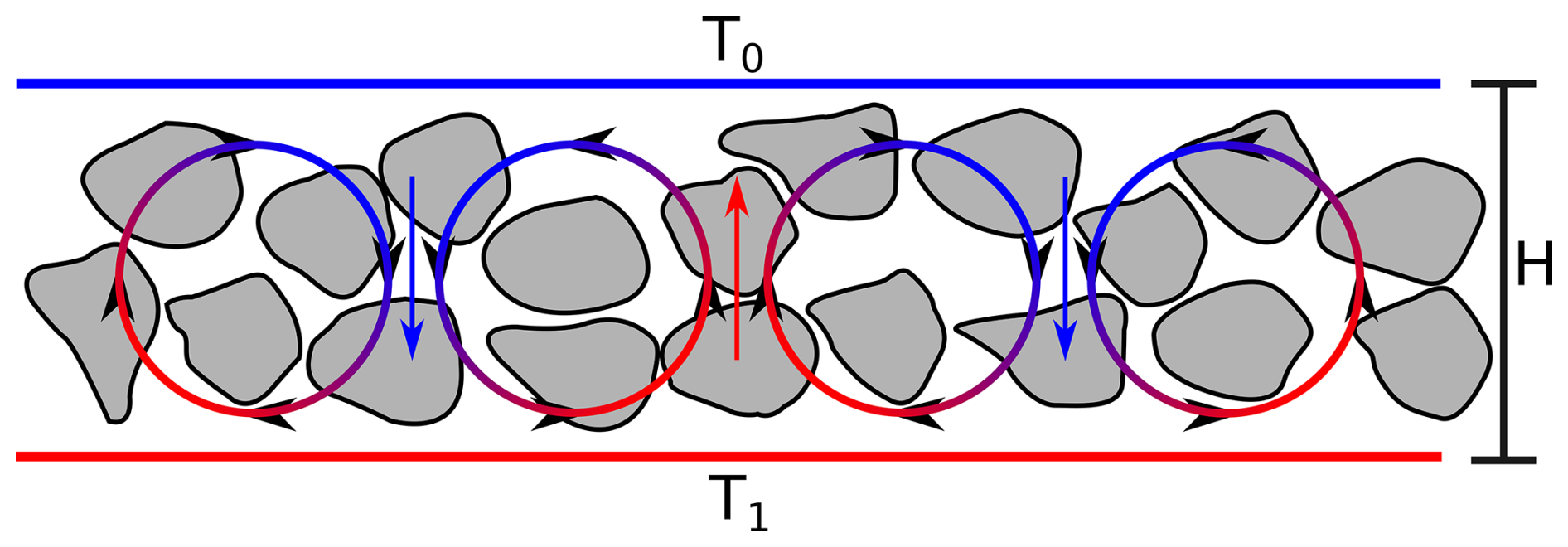
Figure 1 Density-driven air convection. The temperature at the bottom is higher than at the top (T₁>T₀). Adapted from Guodong et al. (2007).

The strength of natural convection in a porous medium is quantified by the Rayleigh–Darcy number (Ra) (Bories and Combarnous, 1973; Otero et al., 2004):

$$\begin{array}{}\text{(1)}& {\displaystyle }{\displaystyle }\mathit{Ra}=g{\displaystyle \frac{{\mathit{\beta }}_{\mathrm{a}}{\mathit{\rho }}_{\mathrm{a}}{c}_{\mathrm{a}}k}{{\mathit{\nu }}_{\mathrm{a}}\mathit{\lambda }}}\mathrm{\Delta }{T}_{\mathrm{a}}H,\end{array}$$

where g (m s⁻²) is the gravitational acceleration; β_a (K⁻¹) is the volumetric thermal expansion coefficient of the air; ρ_a (kg m⁻³), c_a ($\mathrm{J}{\mathrm{kg}}^{-\mathrm{1}}{\mathrm{K}}^{-\mathrm{1}}$), and ν_a (m² s⁻¹) are the density, specific heat capacity, and kinematic viscosity of the air, respectively; k (m²) is the medium permeability; λ ($\mathrm{W}{\mathrm{m}}^{-\mathrm{1}}{\mathrm{K}}^{-\mathrm{1}}$) is the thermal conductivity of the medium; and ΔT_a (K) is the difference in air temperature between two plains separated by a distance H (m). The onset of natural convection is defined by the critical Rayleigh number (Ra_c), which ranges from 27 to 40 depending on the upper-surface characteristics (Lapwood, 1948). The lower limit can be considered to be representative of an open surface (e.g. coarse surface sediments without snow cover), whereas the upper limit can be taken to be representative of an upper surface impermeable to airflow (e.g. coarse surface sediments with thick snow cover).

The Rayleigh number is particularly sensitive to the permeability of the porous medium, which can vary by several orders of magnitude for natural materials depending on the characteristic grain size (Nield and Bejan, 2017). Permeability is commonly estimated using the Kozeny–Carman equation:

$$\begin{array}{}\text{(2)}& {\displaystyle }{\displaystyle }k=A{d}_{\mathrm{10}}^{\mathrm{2}}{\displaystyle \frac{n^{\mathrm{3}}}{(\mathrm{1}-n{)}^{\mathrm{2}}}},\end{array}$$

where d₁₀ (m) is a characteristic grain diameter such that 10 % of the sediment particles are finer than d₁₀, n is the porosity, and $A=\mathrm{0.0056}/\mathrm{4.25}$ is a constant proposed by Côté et al. (2011) that improves the estimation of permeabilities for coarse sediments.

Natural convection in coarse sediments has a strong seasonal variability resulting from air temperature fluctuations. In winter, temperatures inside the sediments are higher than the external air temperature. Air convection intensifies the energy exchange with the atmosphere, causing the sediments to lose energy to the air. In summer, the opposite happens; the temperature inside the sediments is lower than the external air. Since the cold air is heavier than the exterior air, no air convection occurs, and energy exchange is controlled by conduction. The small contact areas between the sediments and the low thermal conductivity of the air result in the sediments acting as a thermal insulator, reducing the amount of energy gained by the ground from the atmosphere (Gruber and Hoelzle, 2008). Over the year, the imbalance of increased energy losses in winter and reduced energy gains in summer produces a net energy loss, lowering the average ground temperature (Guodong et al., 2007).

2.2 GEOtop

GEOtop is a versatile 3D hydrological model that effectively integrates ground energy and water budgets while accounting for atmospheric energy exchange and a multilayer snowpack (Endrizzi et al., 2014; Rigon et al., 2006; Bertoldi et al., 2006; Dall'Amico et al., 2011). This makes it suitable for modelling permafrost-relevant variables such as snow and ground temperatures. This work refers to GEOtop 3.0 as the standard GEOtop (S-GEOtop). The system of equations for the water flow and energy balance in S-GEOtop is as follows:

$$\begin{array}{}\text{(3)}& {\displaystyle }& {\displaystyle \frac{\partial {\mathrm{\Phi }}_m}{\partial t}}+\mathrm{\nabla }\cdot {\mathit{J}}_{\mathrm{w}}+F_{\mathrm{w}}=\mathrm{0},\text{(4)}& {\displaystyle }& {\displaystyle \frac{\partial U}{\partial t}}+{\displaystyle \frac{\partial G}{\partial z}}=\mathrm{0},\end{array}$$

where ${\mathrm{\Phi }}_m=\frac{M_{\mathrm{w}}+M_{\mathrm{i}}}{{\mathit{\rho }}_{\mathrm{w}}{V}_{\mathrm{c}}}$ is a dimensionless variable representing total water content expressed as liquid water, with M_w and M_i being the mass of liquid water and ice, respectively; ρ_w (kg m⁻³) being the density of liquid water; and V_c (m³) being a control volume. ${\mathit{J}}_{\mathrm{w}}=-\frac{k_{\text{rw}}k}{{\mathit{\mu }}_{\mathrm{w}}}(\mathrm{\nabla }P-{\mathit{\rho }}_{\mathrm{w}}\mathit{g})$ (m s⁻¹) is the water flux, with k_rw being the relative permeability of water, μ_w (Pa s) being the dynamic viscosity of liquid water, ∇P (Pa m⁻¹) being the pressure gradient, and g (m s⁻²) being the gravity vector. F_w (s⁻¹) is a sink term representing evapotranspiration, which can act in the first layers of the sediments. $U=C_{\mathrm{m}}(T-T_{\text{ref}})+{\mathit{\rho }}_{\mathrm{w}}{L}_{\mathrm{f}}{\mathit{\theta }}_{\mathrm{w}}$ (J m⁻³) is the internal energy, where C_m ($\mathrm{J}{\mathrm{m}}^{-\mathrm{3}}{\mathrm{K}}^{-\mathrm{1}}$) is the medium volumetric heat capacity, T (K) is the temperature within V_c, T_ref is a reference temperature, L_f (J Kg⁻¹) is the latent heat of fusion, and θ_w is the volumetric liquid water content. $G=-{\mathit{\lambda }}_{\mathrm{T}}\frac{\partial T}{\partial z}$ (W m⁻²) represents the vertical component of the conduction flux, where λ_T ($\mathrm{W}{\mathrm{m}}^{-\mathrm{1}}{\mathrm{K}}^{-\mathrm{1}}$) is the effective thermal conductivity within V_c.

Prior research has utilized S-GEOtop in mountain regions to model snow cover (Dall'Amico et al., 2018), water and energy fluxes (Rigon et al., 2006; Soltani et al., 2019), and permafrost distribution (Wani et al., 2021; Fiddes et al., 2015). However, as the model does not consider airflow in porous media, it fails to accurately represent the thermal behaviour of coarse sediments, leading to inaccurate representation of permafrost distribution in mountain landforms such as talus slopes, moraines, and rock glaciers.

2.3 Convection-enhanced GEOtop

2.3.1 Governing equations

To incorporate natural convection into the S-GEOtop model, a new set of transport equations is implemented to solve for the airflow within the sediments and the air heat transport, creating a new model version referred to as convection-enhanced GEOtop (CE-GEOtop). While the S-GEOtop formulation assumes that all phases are in thermal equilibrium within a control volume (Fig. 2a), CE-GEOtop uses the local thermal non-equilibrium (LTNE) approach to characterize the energy balance of the air phase (Yang et al., 2012; Su and Davidson, 2015).

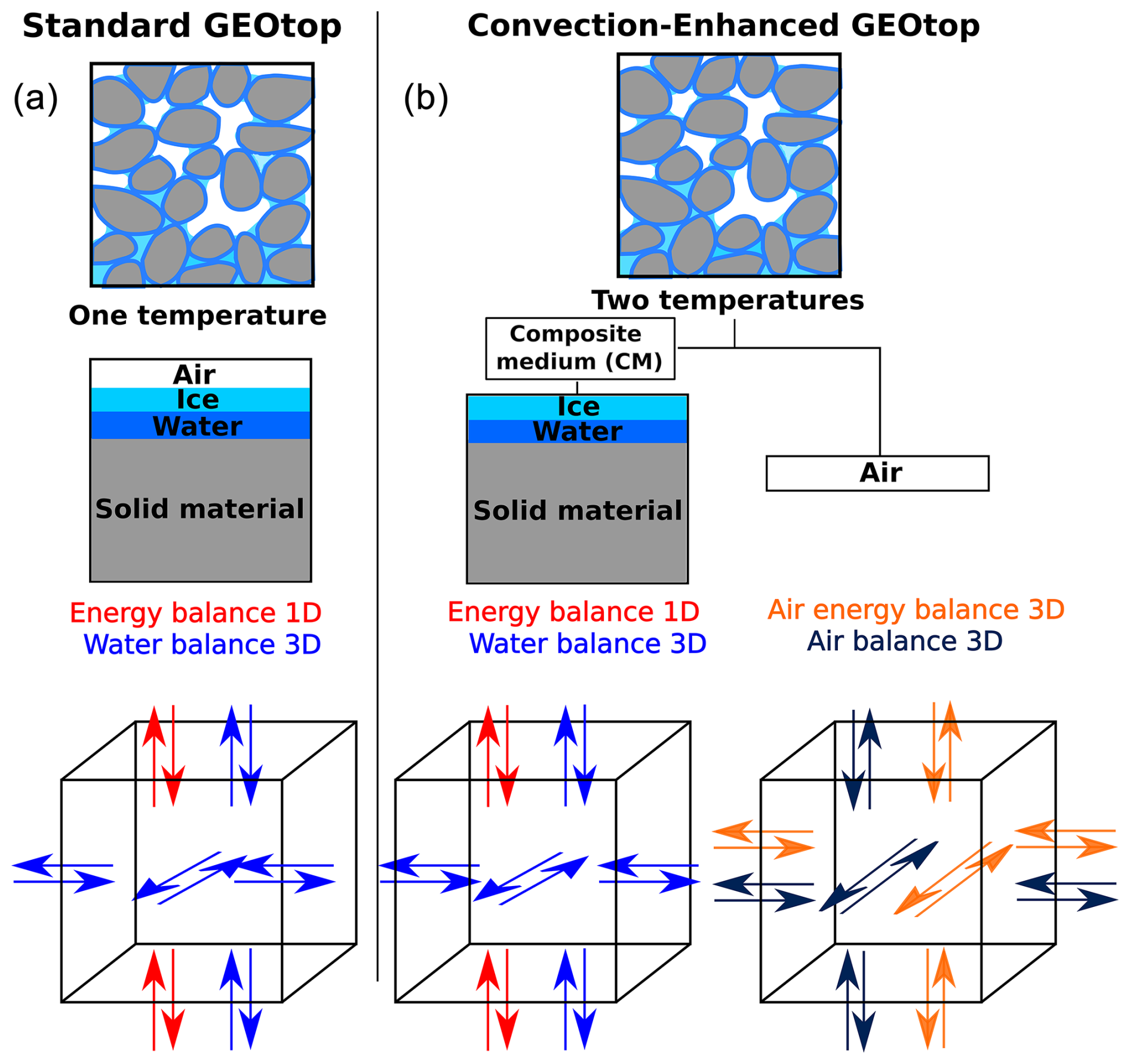
Figure 2 (a) The conceptual model of the standard GEOtop model. (b) The conceptual model of the convection-enhanced GEOtop model.

According to this approach, the air temperature differs from the temperature of the other phases in the control volume (Fig. 2b). In this context, the group of all non-air phases will be referred to as the composite medium (CM). These phases are considered to be in local thermal equilibrium (LTE), as in the original implementation of S-GEOtop, meaning that for each control volume, the new model will keep track of two different temperatures and the heat transfer processes between these two main phases. Although the LTNE approach requires additional parameters to determine the inter-phase heat transfer, it explicitly accounts for the decoupling between the temperature of the air phase and the CM, leading to a more realistic representation of convective heat transfer.

Analogously to the water mass balance, the air mass balance is formulated using Richards' equation, with the key distinction that air density is now temperature-dependent to account for buoyancy forces driving natural convection. The airflow equation is solved using the Oberbeck–Boussinesq approximation, which treats air flux as incompressible (Eq. 5) while retaining density variation solely within Darcy's law (Barletta, 2009; Landman and Schotting, 2007). This assumption is commonly applied in systems where pressure or temperature changes are not significant, simplifying the numerical solution. However, neglecting air compressibility may limit the model's applicability in cases dominated by strong vertical gradients. Regarding external pressure, the model assumes it increases with elevation and influences boundary conditions but does not affect air density. As detailed in Appendix A2, the airflow equations are expressed as

$$\begin{array}{}\text{(5)}& {\displaystyle }& {\displaystyle }{\mathit{\rho }}_{\mathrm{a}}\mathrm{\nabla }\cdot {\mathit{V}}_{\mathrm{a}}=\mathrm{0},\text{(6)}& {\displaystyle }& {\displaystyle }{\mathit{V}}_{\mathrm{a}}={\displaystyle \frac{k_{\text{ra}}k}{{\mathit{\mu }}_{\mathrm{a}}}}(\mathrm{\nabla }P-{\mathit{\rho }}_{\mathrm{a}}\mathit{g}),\end{array}$$

where V_a (m s⁻¹) is the air velocity, k_ra is the relative permeability of the air, and μ_a (Pa s) is the dynamic viscosity of air. The air density is calculated as ${\mathit{\rho }}_{\mathrm{a}}\left(T_{\mathrm{a}}\right)={\mathit{\rho }}_{\mathrm{a}}\left(T_{\text{ref}}\right)\left[\mathrm{1}-\mathit{\beta }\cdot (T_{\mathrm{a}}-T_{\text{ref}})\right]$ (Nield and Bejan, 2017). k_ra is calculated by the van Genuchten approach as proposed by Mahabadi et al. (2016), which uses the same parameters for both the water and the air relative permeabilities:

$$\begin{array}{}\text{(7)}& {\displaystyle }{\displaystyle }{k}_{\text{ra}}=(\mathrm{1}-{\overline{S}}_{\mathrm{a}}{)}^{\mathrm{0.5}}{\left[\mathrm{1}-{\overline{S}}_{\mathrm{a}}^{\mathrm{1}/m}\right]}^{\mathrm{2}m},{\overline{S}}_{\mathrm{a}}={\displaystyle \frac{S_{\mathrm{w}}-S_{\text{rw}}}{\mathrm{1}-S_{\text{rw}}}},\end{array}$$

where S_rw is the residual water saturation, m is a van Genuchten parameter, and $S_{\mathrm{w}}=\frac{{\mathit{\theta }}_{\mathrm{w}}}{n}$ is the relative liquid water content. To solve Eq. (5), the lateral and bottom domain boundaries are assumed to be impermeable, whereas the top boundary condition is snow-dependent; in snow-free pixels, an open boundary condition is applied, allowing air exchange between the soil and the atmosphere, while a no-flux boundary is applied to snow-covered pixels. Some authors have reported air infiltration in the soil even with snow cover up to 0.5–1 m (Delaloye and Lambiel, 2005; Scherler et al., 2013; Morard et al., 2008; Amschwand et al., 2024); therefore, a threshold parameter, H_ai (m), is included to account for potential air infiltration in snow-covered pixels. For snow depths below H_ai, the airflow remains unimpeded by snow cover (open boundary condition).

The energy transport equation in the air phase combines advection and conduction processes:

$$\begin{array}{}\text{(8)}& {\displaystyle }{\displaystyle \frac{\partial U_{\mathrm{a}}}{\partial t}}+\mathrm{\nabla }\cdot ({\mathit{G}}_{\mathrm{a}}+{\mathit{J}}_{\mathrm{a}})-h(T_{\text{cm}}-T_{\mathrm{a}})=\mathrm{0},\end{array}$$

where $U_{\mathrm{a}}=C_{\mathrm{a}}(T_{\mathrm{a}}-T_{\text{ref}})$ (J m⁻³) is the air internal energy, T_a (K) and T_cm (K) are the temperatures of the air and the composite medium, respectively, and C_a ($\mathrm{J}{\mathrm{m}}^{-\mathrm{3}}{\mathrm{K}}^{-\mathrm{1}}$) is the air volumetric heat capacity. The heat conduction flux is denoted by ${\mathit{G}}_{\mathrm{a}}=-{\mathit{\lambda }}_{\mathrm{a}}\mathrm{\nabla }{T}_{\mathrm{a}}$ (W m⁻²), where λ_a ($\mathrm{W}{\mathrm{m}}^{-\mathrm{1}}{\mathrm{K}}^{-\mathrm{1}}$) is the air thermal conductivity, while the heat advected by the airflow is given by ${\mathit{J}}_{\mathrm{a}}={\mathit{\rho }}_{\mathrm{a}}{C}_{\mathrm{a}}(T_{\mathrm{a}}-T_{\text{ref}}){\mathit{V}}_{\mathrm{a}}$ (W m⁻²). Lastly, h ($\mathrm{W}{\mathrm{m}}^{-\mathrm{3}}{\mathrm{K}}^{-\mathrm{1}}$) is a heat transfer coefficient describing the heat exchange between the air and the composite medium. For a proper representation of the coupling between the two phases, the heat exchange term included in Eq. (8) should be included with the opposite sign in the energy balance for the composite medium (Eq. 4). Following the approach proposed by Su and Davidson (2015), the heat transfer coefficient h is calculated as

$$\begin{array}{}\text{(9)}& {\displaystyle }{\displaystyle }h={\displaystyle \frac{A_{\mathrm{p}}{h}_{\text{cm–a}}(\mathrm{1}-{\mathit{\theta }}_{\mathrm{a}})}{V_{\mathrm{p}}}},\end{array}$$

where A_p (m²) and V_p (m³) are the surface area and volume, respectively, of a spherical particle with diameter d_p, θ_a is the air content, and h_cm–a ($\mathrm{W}{\mathrm{m}}^{-\mathrm{2}}{\mathrm{K}}^{-\mathrm{1}}$) is the heat transfer coefficient between the CM and the air interface calculated as

$$\begin{array}{}\text{(10)}& {\displaystyle }{\displaystyle }{h}_{\text{cm–a}}={\displaystyle \frac{{\mathit{Nu}}_{\text{sa}}{\mathit{\lambda }}_{\mathrm{a}}}{d_{\mathrm{p}}}}.\end{array}$$

In the previous expression, Nu_sa is the solid-to-air Nusselt number, which is expressed as

$$\begin{array}{}\text{(11)}& {\displaystyle }{\displaystyle }{\mathit{Nu}}_{\text{sa}}=a+b\cdot {\mathit{\text{Pr}}}_{\mathrm{a}}^{\mathrm{1}/\mathrm{3}}\cdot {\mathit{\text{Re}}}_{\mathrm{p}}^c,\end{array}$$

where ${\mathit{\text{Re}}}_{\mathrm{p}}=\frac{\left|{\mathit{V}}_{\mathrm{a}}\right|d_{\mathrm{p}}}{{\mathit{\nu }}_{\mathrm{a}}}$ is the particle Reynolds number and Pr_a is the air Prandtl number. At atmospheric pressure, Pr_a is fairly constant for temperatures between −10 and 25 °C, so a constant value of Pr_a=0.711 is used, corresponding to its value for 0 °C. In Eq. (11), the coefficients a, b, and c are the heat transfer model constants; for packed spheres, they were estimated to be a=2, b=0.5, and $c=\mathrm{1}/\mathrm{3}$ (Whitaker, 1977).

2.3.2 Thermal conductivity

Thermal conductivity plays a fundamental role in the sediment's conductive heat transport and, thus, in the exchange of heat with the atmosphere. Particularly, the low thermal conductivity of coarse sediments leads to an overall decrease in ground temperatures (Gruber and Hoelzle, 2008). Currently, S-GEOtop calculates the sediment's effective thermal conductivity λ_T, using the approach proposed by Cosenza et al. (2003):

$$\begin{array}{}\text{(12)}& {\displaystyle }{\displaystyle }{\mathit{\lambda }}_{\mathrm{T}}={\left[(\mathrm{1}-n)\sqrt{{\mathit{\lambda }}_{\mathrm{s}}}+{\mathit{\theta }}_{\mathrm{w}}\sqrt{{\mathit{\lambda }}_{\mathrm{w}}}+{\mathit{\theta }}_{\mathrm{i}}\sqrt{{\mathit{\lambda }}_{\mathrm{i}}}+{\mathit{\theta }}_{\mathrm{a}}\sqrt{{\mathit{\lambda }}_{\mathrm{a}}}\right]}^{\mathrm{2}},\end{array}$$

where θ_i is the volumetric fraction of ice, λ_s the thermal conductivity of sediment particles, λ_w the thermal conductivity of water, and λ_i the thermal conductivity of ice. This approach generally leads to a reasonable estimation of the sediments' thermal conductivity, although it overestimates the conductivity in dry conditions. Using Eq. (12), the minimum thermal conductivity is ${\mathit{\lambda }}_{\mathrm{T}}=\left[\right(\mathrm{1}-n)\sqrt{{\mathit{\lambda }}_{\mathrm{s}}}+{\mathit{\theta }}_{\mathrm{a}}\sqrt{{\mathit{\lambda }}_{\mathrm{a}}}{]}^{\mathrm{2}}\sim \mathrm{0.9}$ $\mathrm{W}{\mathrm{m}}^{-\mathrm{1}}{\mathrm{K}}^{-\mathrm{1}}$ for a case with negligible water content, porosity of 40 %, and solid thermal conductivity of 2.2 $\mathrm{W}{\mathrm{m}}^{-\mathrm{1}}{\mathrm{K}}^{-\mathrm{1}}$. However, previous authors have shown that for liquid water contents lower than 5 %–10 %, λ_T∼0.3–0.5 $\mathrm{W}{\mathrm{m}}^{-\mathrm{1}}{\mathrm{K}}^{-\mathrm{1}}$ (Bristow, 2018; Côté and Konrad, 2009), which is about the half of the value estimated using Eq. (12). These low thermal conductivities under dry conditions occur since the rock-to-rock contacts are minimal due to the rock roughness (Cheng and Wong, 2022). Those small open spaces on the rock-to-rock contact are filled with air for dry conditions, hindering thermal conduction (Bristow, 2018).

In CE-GEOtop, a new approach to calculating the thermal conductivity was implemented. Particularly, the estimation of the thermal conductivity for low-water-content conditions is improved using the Farouki–de Vries model (Farouki, 1981; Tian et al., 2016):

$$\begin{array}{}\text{(13)}& {\displaystyle }{\mathit{\lambda }}_{\mathrm{T}}={\displaystyle \frac{{\mathit{\theta }}_{\mathrm{w}}\cdot {\mathit{\lambda }}_{\mathrm{w}}+w_{\mathrm{i}}\cdot {\mathit{\theta }}_{\mathrm{i}}\cdot {\mathit{\lambda }}_{\mathrm{i}}+w_{\mathrm{a}}\cdot {\mathit{\theta }}_{\mathrm{a}}\cdot {\mathit{\lambda }}_{\mathrm{a}}+w_{\mathrm{s}}\cdot (\mathrm{1}-n)\cdot {\mathit{\lambda }}_{\mathrm{s}}}{{\mathit{\theta }}_{\mathrm{w}}+w_{\mathrm{i}}\cdot {\mathit{\theta }}_{\mathrm{i}}+w_{\mathrm{a}}\cdot f_{\mathrm{a}}+w_{\mathrm{s}}\cdot (\mathrm{1}-n)}},\text{(14)}& {\displaystyle }\begin{array}{rl}{w}_n& ={\displaystyle \frac{\mathrm{2}\cdot g_n}{\mathrm{3}}}{\left[\mathrm{1}+\left({\displaystyle \frac{{\mathit{\lambda }}_n}{{\mathit{\lambda }}_{\mathrm{w}}}}-\mathrm{1}\right)\right]}^{-\mathrm{1}}\\ & +{\displaystyle \frac{\mathrm{1}}{\mathrm{3}}}{\left[\mathrm{1}+\left({\displaystyle \frac{{\mathit{\lambda }}_n}{{\mathit{\lambda }}_{\mathrm{w}}}}-\mathrm{1}\right)\left(\mathrm{1}-\mathrm{2}{g}_n\right)\right]}^{-\mathrm{1}},n\in \mathit{\{}a,i,s\mathit{\}},\end{array}\end{array}$$

where w_n denotes the weighting factors of air (a), ice (i), and solid particles, respectively. g_n denotes the shape factors of the individual phases, where uniform shape factors $g_{\mathrm{i}}=g_{\mathrm{s}}=\mathrm{0.125}$ are adopted for ice and solid particles, while the shape factor of air (g_a) depends on the water content:

$$\begin{array}{}\text{(15)}& {\displaystyle }{\displaystyle }{g}_{\mathrm{a}}=\left\{\begin{array}{ll}\mathrm{0.333}-(\mathrm{0.333}-\mathrm{0.035}){\mathit{\theta }}_{\mathrm{a}}/n& \text{if }{\mathit{\theta }}_{\mathrm{w}}\ge \mathrm{0.09},\\ \mathrm{0.013}+\mathrm{0.944}{\mathit{\theta }}_{\mathrm{w}}& \text{if }{\mathit{\theta }}_{\mathrm{w}}<\mathrm{0.09}.\end{array}\right.\end{array}$$

The Farouki–de Vries model sets liquid water as the continuum medium and sediment minerals as uniform particles to estimate λ_T of unfrozen and frozen soil. Under the same dry conditions mentioned earlier, the Farouki–de Vries model will predict thermal conductivity of λ_T=0.32 $\mathrm{W}{\mathrm{m}}^{-\mathrm{1}}{\mathrm{K}}^{-\mathrm{1}}$, which is consistent with the reported sediment's thermal conductivity for dry conditions (λ_T∼0.3–0.5 $\mathrm{W}{\mathrm{m}}^{-\mathrm{1}}{\mathrm{K}}^{-\mathrm{1}}$; Bristow, 2018; Côté and Konrad, 2009).

One of the limitations of the CE-GEOtop model for simulating the thermal dynamics of coarse sediments is its exclusion of thermal radiation effects. Although some methods exist for estimating radiation in dry, coarse sediments (e.g. Fillion et al., 2011), the influence of water and ice content on thermal radiation requires further attention.

2.3.3 Numerical solver

The four main transport equations are solved sequentially in a time-lagged manner (Panday and Huyakorn, 2004): (i) air mass balance (Eq. 5), (ii) air energy balance (Eq. 8), (iii) composite-medium energy balance (Eq. 4), and (iv) water mass balance (Eq. 3). Each equation is solved using the implicit finite-volume scheme originally implemented in S-GEOtop. The solver is based on a Newton–Raphson iterative scheme (more details in Appendix A1).

Given the non-linear nature of the system of equations, maintaining control over the numerical convergence of the simulation becomes crucial. Arenson et al. (2006), in their study involving air convection simulations, underscored the challenge of establishing an appropriate relationship between the medium permeability and the numerical resolution parameters (time step and mesh spacing). They emphasized that numerical instabilities may arise rapidly when these factors are not adequately balanced.

In the CE-GEOtop, a mechanism has been implemented to monitor the stability of the numerical solution using the maximum grid Courant number for the air velocities (Cu):

$$\begin{array}{}\text{(16)}& {\displaystyle }{\displaystyle }\mathit{Cu}=\text{max}\left(\left\{\mathrm{\Delta }t{\displaystyle \frac{{\mathit{V}}_{\mathrm{a}}}{\mathrm{\Delta }d}}{\mathrm{|}}_i,i=\mathrm{1},\mathrm{\dots },N\right\}\right),\end{array}$$

where V_a|_i, and Δd|_i are the air velocity and spacing, respectively, at the ith face of the grid and N is the number of faces in the grid. At each iteration, the model examines the Cu and reduces the Δt if Cu surpasses the user-defined maximum value, Cu_max. Despite the utilization of an implicit numerical scheme, it is generally advised to maintain Cu_max<10 to ensure both stability and accuracy of the numerical solution (Rai and Chakravarthy, 1986).

2.3.4 Shadows

Radiation plays an important role in the ground–surface energy balance. In complex terrain, careful considerations are necessary for an accurate estimation of the total radiation that the surface receives. S-GEOtop accounts for both cast shadows from surrounding topography and the view factor's impact on radiation (Endrizzi et al., 2014). However, during the development of the new code, it was detected that the method for calculating cast shadows could be improved to provide a more accurate estimation of the shadows in rugged terrain. The original approach in S-GEOtop uses the model digital elevation mode (DEM) to calculate cast shadows, but it often fails to account for shadows cast from peaks outside the model's domain. In CE-GEOtop, this limitation is addressed by allowing for the input of a second larger DEM specifically for calculating cast shadows. This enhancement improves the model's capacity to represent shadow conditions without expanding the model's dimensions.

3 Case study – Babylon talus slope

To evaluate CE-GEOtop's performance in a realistic scenario, the model is applied to the Babylon talus slope in the Lake O'Hara watershed, Yoho National Park, Canada, where field evidence suggests permafrost presence (Fig. 3). The Babylon basin is approximately 0.28 km² in surface area and is drained by Babylon Creek, which exits the northeast corner of the basin.

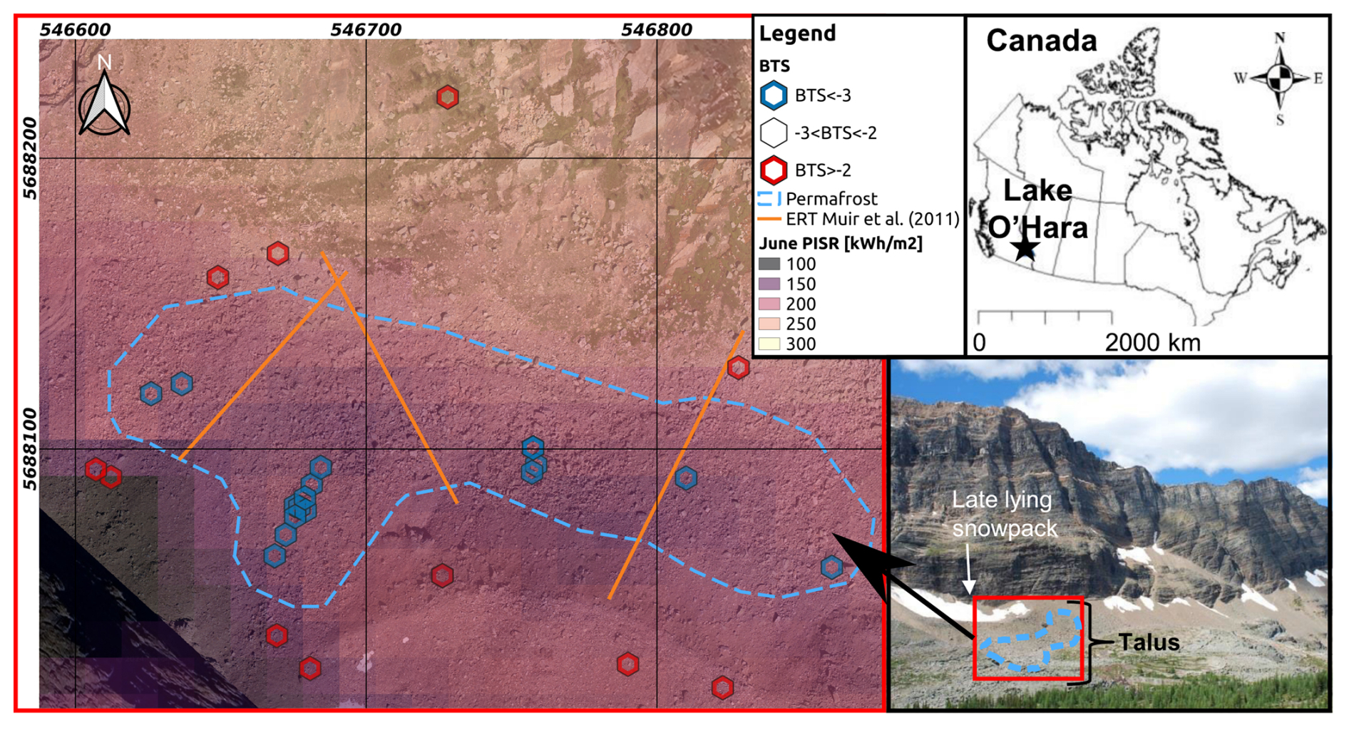
Figure 3 Map of Babylon talus slope showing the locations of basal temperature (BTS) sensors (hexagons), electrical resistivity tomography profiles (orange lines), and estimated permafrost extent (blue line). June potential incoming solar radiation (PISR) was calculated using SAGA GIS (version 2.3.1; http://saga-gis.org, last access: November 2023) and the satellite digital elevation model ALOS PALSAR (12.5 m×12.5 m: JAXA/METI ALOS PALSAR L1.0 2007).

The bedrock underlying the talus is from the Lower Cambrian Gog Group, mainly consisting of quartzite, while Middle Cambrian carbonates cap the peaks surrounding the watershed (Price et al., 1980). The talus is predominantly composed of cobble- to boulder-sized rocks, and geophysical surveys combined with hydrograph analysis indicate an openwork matrix with large void spaces without the presence of fine material (Muir et al., 2011). This coarse, blocky surface supports only sparse vegetation, making it difficult to infer thermally anomalous zones from vegetation patterns.

Meteorological data from a nearby weather station show that the mean monthly air temperature in the area ranges from −9.7 °C in January to 10.4 °C in July, with annual precipitation of 1000–1200 mm, predominantly in the form of snow (He and Hayashi, 2019). Two small springs at the base of the Babylon talus flow toward Babylon Creek along the bedrock plane. Discharge and temperature were measured weekly at Babylon Creek from July to September 2008, with continuous stage recording every 10 min using pressure transducers in a stilling well (AquaTroll 200, In-Situ Inc.; Muir et al., 2011). Discharge was estimated using a stage–discharge rating curve developed from manual water stage measurements.

In specific sections of the Babylon talus slope, high electrical resistivity values exceeding 50 kΩ m were observed (Muir et al., 2011), indicating the presence of permafrost (Hauck and Kneisel, 2008). To verify this, surface temperature sensors (iButtons DL1925 and DS1921Z-F5) were deployed during the winter seasons of 2016, 2021, and 2022. By correlating high-resistivity zones with low basal temperatures of the snowpack (BTS), permafrost was identified in the middle–bottom section of the Babylon talus slope (Fig. 3). The presence of permafrost in the middle–bottom section of the talus and within coarser sediments suggests that natural convection influences permafrost occurrence at the Babylon talus slope, making it an interesting case study for evaluating CE-GEOtop under actual field conditions.

4 Results and discussions

Thoroughly evaluating the CE-GEOtop model presents a challenge due to the absence of an analytical solution encompassing all the processes the model accounts for. Nonetheless, the standard GEOtop model has been validated by previous studies (Endrizzi et al., 2014; Dall'Amico et al., 2011); hence, this study will focus on a comparative analysis of the new air convection module in CE-GEOtop with respect to equivalent simulations performed with S-GEOtop. This section begins by examining the effects of local thermal non-equilibrium (LTNE) using a synthetic case. Following this, the performance of the air convection module is assessed on the Babylon talus slope.

4.1 Effect of Rayleigh number and local thermal non-equilibrium (LTNE)

Simulations using CE-GEOtop were conducted to evaluate the differences between a case considering the classical LTE assumption and a case using the LTNE approach. These simulations evaluated the impact of considering different heat transport processes in the sediment's temperature without considering surface energy fluxes. The LTE simulations were achieved by artificially increasing the heat transfer term (h; Eq. 9), thus enforcing the same temperature between the air and the composite medium. Additionally, S-GEOtop simulations were performed to establish a baseline for comparison with CE-GEOtop. Since S-GEOtop exclusively considers conduction as the heat transport mechanism, any agreement between the results of CE-GEOtop and S-GEOtop implies the absence of natural convection.

The numerical experiment involved a synthetic geometry representing a flat square domain with dimensions of 33 m by 33 m and a 3 m layer of coarse sediments with a permeability of $\mathrm{1.0}\times {\mathrm{10}}^{-\mathrm{6}}$ m² (d₁₀∼70 mm). The domain was discretized into 12 vertical layers of 0.25 m each and a grid size of 1.5 m, resulting in 22 grid cells in both the longitudinal and the transversal directions.

To limit the interaction with the atmosphere, the surface energy balance was removed, which included eliminating shortwave and longwave radiation (by setting surface albedo to 1 and surface emissivity to 0), latent heat (by setting sediment water content to θ_w=0 and using a low air relative humidity), and sensible heat (by setting a low wind velocity). The sediments were initialized with a temperature of 15 °C, and a no-flux lower boundary condition was applied for the heat transfer. On the top boundary, a fixed temperature (T_top) was applied to the sediments and air throughout the simulation. The simulations were carried out for various values of T_top, resulting in a range of Rayleigh numbers from 25 to 265. With a lower impermeable boundary and an upper open surface, Ra_c was estimated to be 27 (Lapwood, 1948). The simulations were conducted with constant boundary conditions over a period of 30 d. The results were analyzed in terms of the layer-averaged normalized temperature $T_t^{*}\left(z\right)$:

$$\begin{array}{}\text{(17)}& {\displaystyle }{\displaystyle }{T}_t^{*}\left(z\right)={\displaystyle \frac{\stackrel{\mathrm{‾}}{T_t\left(z\right)}-T_{\text{top}}}{T_{\text{ini}}-T_{\text{top}}}},\end{array}$$

where $\stackrel{\mathrm{‾}}{T_t\left(z\right)}$ (K) is the temperature average over the layer at time t (s) and T_ini (K) is the initial temperature.

All simulations exhibit identical temperature profiles for the lowest Rayleigh number (Ra=25), indicating the absence of natural convection (Fig. 4). However, with a slightly higher Rayleigh number (Ra=65), natural convection influences the sediment temperature profiles after approximately 15–20 d in the LTNE simulation. This suggests that although the Rayleigh number exceeds its critical value, natural convection is not strong enough to affect ground temperatures over short periods. Analysis of the results of the higher Ra values reveals that natural convection becomes increasingly significant for Ra>100 as evidenced by the temperature profiles while considering the LTNE approach.

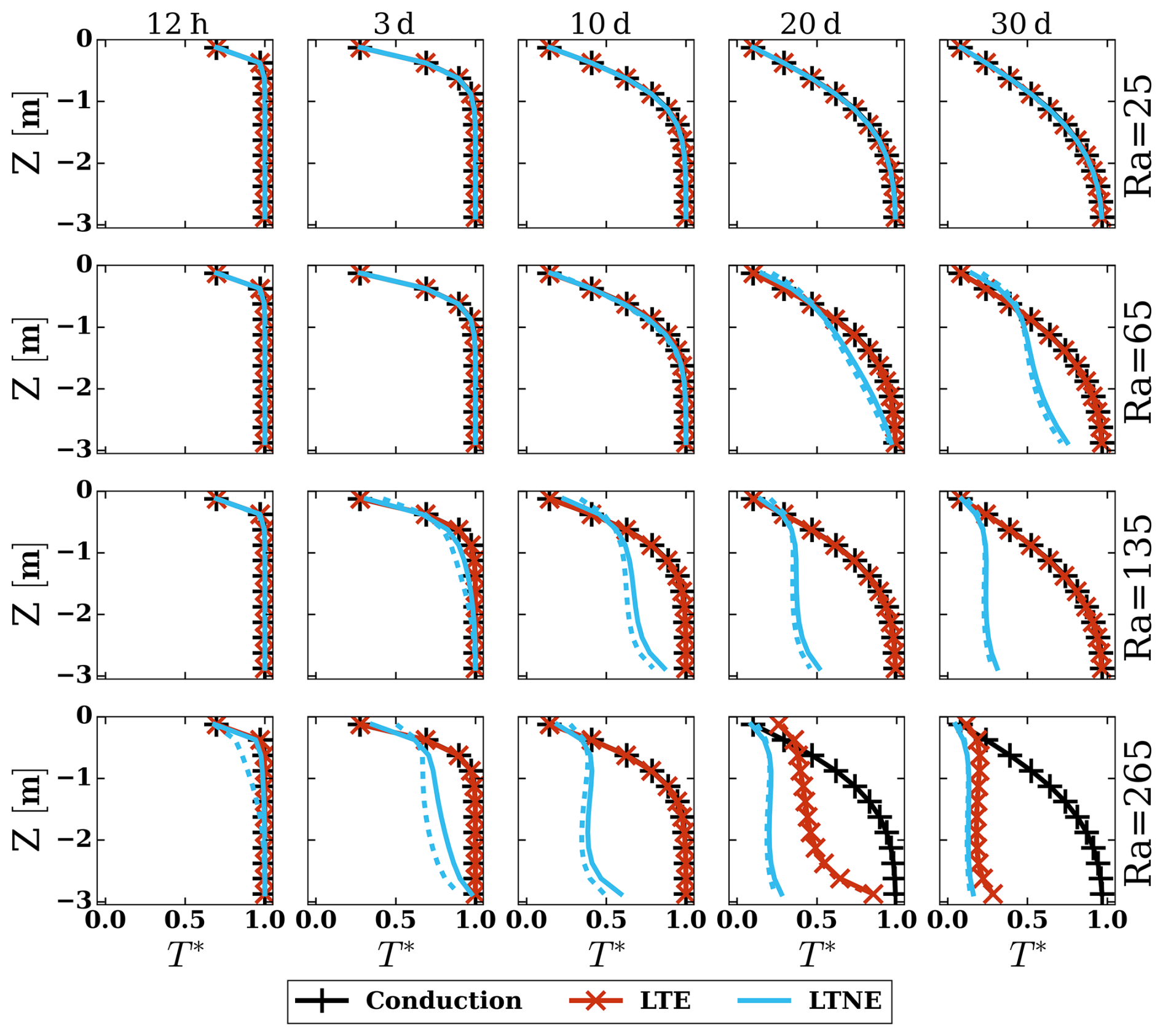
Figure 4 Layer-averaged temperature profiles for different Ra values plotted against normalized temperature (T^*) for S-GEOtop (conduction only), CE-GEOtop (LTE), and CE-GEOtop (LTNE). The solid lines represent the sediment temperature, and the dashed lines represent the air temperature.

At monthly timescales, the LTE simulations are indistinguishable from the pure conduction simulations in all cases except for Ra=265. In this last case with the highest Rayleigh number, LTE simulations show lower temperatures than the pure conduction case after 20 d and eventually resemble the LTNE simulations after 30 d, indicating that the system reaches local thermal equilibrium. However, significant disparities are observed for shorter times or lower Rayleigh numbers, highlighting the system's non-thermal equilibrium state. This is evident in the air temperature profiles for the LTNE case (dashed cyan lines), where early air temperature indicates lower temperatures than those of the sediment. As a result, the thermal non-equilibrium state leads to a faster decrease in the temperature of the sediments. Therefore, adopting the LTE approach affects the short-term response of the sediments' temperature and hinders natural convection effects.

4.2 Thermal anomalies at talus slopes

Topoclimatic factors, such as air temperature and potential incoming solar radiation (PISR), are typically used to delineate permafrost zones. For the Babylon talus slope case study, these variables would suggest that the upper part of the talus is the most favourable zone for the occurrence of permafrost due to the lower air temperatures and PISR. However, the observed permafrost zone is in the middle–bottom part of the talus (Fig. 3), similar to observations in previous studies elsewhere (e.g. Morard et al., 2008; Popescu et al., 2017; Delaloye and Lambiel, 2005; Phillips et al., 2009). This thermal anomaly could be caused by air convection in two characteristic regimes: the winter regime, in which cold external air induces the influx of air into the bottom of the slope and warm air outflow at the top (Fig. 5a), and the summer regime, in which higher external air temperature causes the influx of warm air at the top and the outflow of cold air at the bottom (Fig. 5b). Similar convective patterns can also occur on a diurnal timescale: surface cooling by longwave radiation at night can drive upslope air movement, while daytime heating by shortwave radiation can reverse this flow as surface temperatures rise.

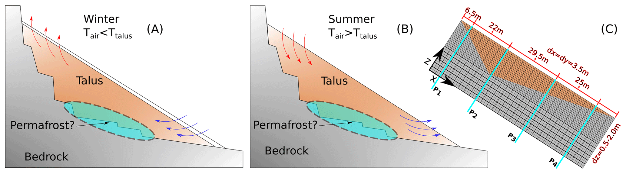
Figure 5 Conceptual model of the talus slope: (a) winter regime and (b) summer regime (modified from Morard et al., 2008); (c) a cross-section of the 3D model along the longitudinal line running in the center of the slope (y=19.25 m), where vertical lines show the positions of temperature profiles (P₁, P₂, P₃, and P₄).

To assess whether the CE-GEOtop model can represent the air convection fluxes on a talus slop, the summer and winter regimes will be simulated. The CE-GEOtop (with LTNE) and S-GEOtop models were configured using the dimensions of the Babylon talus slope with a constant slope angle of 21° derived from a DEM. The 3D model domain is confined within the boundaries of the geophysical survey (Muir et al., 2011), with the talus slope's longitudinal axis measuring 94.5 m and the transversal axis 38.5 m. Figure 5c shows a cross-section of the model along the longitudinal centerline of the slope. The grid size is set at 3.5 m, resulting in 27 grid cells in the longitudinal direction and 12 in the transversal direction. The bedrock depth, based on Muir et al. (2011), reaches a maximum of 16 m at the middle section of the talus slope, gradually decreasing to 0 m at the top and bottom regions. Consequently, the initial 16 m of the sediment domain is discretized into 32 layers, each one with a thickness of 0.5 m, while the subsequent 12 layers representing the bedrock have varying thicknesses ranging from 0.5 to 2 m, in total reaching to a depth of 33.25 m. A constant geothermal heat flux of 0.03 W m⁻² was set as the model's lower boundary condition (Scherler et al., 2013).

For each regime, three cases were run; the first, CG-HK, used the CE-GEOtop model with coarse sediments and a high permeability of $k=\mathrm{1.5}\times {\mathrm{10}}^{-\mathrm{6}}$ m² representing low-end values for cobble-sized materials based on laboratory measurements (Côté et al., 2011). The second is SG-HK, which utilized the standard GEOtop model with coarse sediments ($k=\mathrm{1.5}\times {\mathrm{10}}^{-\mathrm{6}}$ m²). The last one is CG-LK, employing CE-GEOtop with sand-sized sediments with low permeability ($k=\mathrm{1}\times {\mathrm{10}}^{-\mathrm{10}}$ m²) instead of coarse sediments. For all cases, bedrock is assumed to be almost impermeable with $k=\mathrm{2}\times {\mathrm{10}}^{-\mathrm{15}}$ m² (Hayashi, 2020).

Although CE-GEOtop is capable of incorporating fully time-varying meteorological forcings, the summer and winter regime simulations were conducted with constant boundary conditions for 10 d to isolate the direct effects of higher or lower air temperatures on airflow patterns. As in the preceding simulations, all surface energy balance terms were neglected.

4.2.1 Winter regime

The talus and bedrock's initial temperature were set to T=10 °C, whereas the external air temperature was set to 2.5 °C. Figure 6 compares the simulated temperatures at four different profiles located along the center line of the model domain: P₁, P₂, P₃, and P₄ (see Fig. 5c for locations).

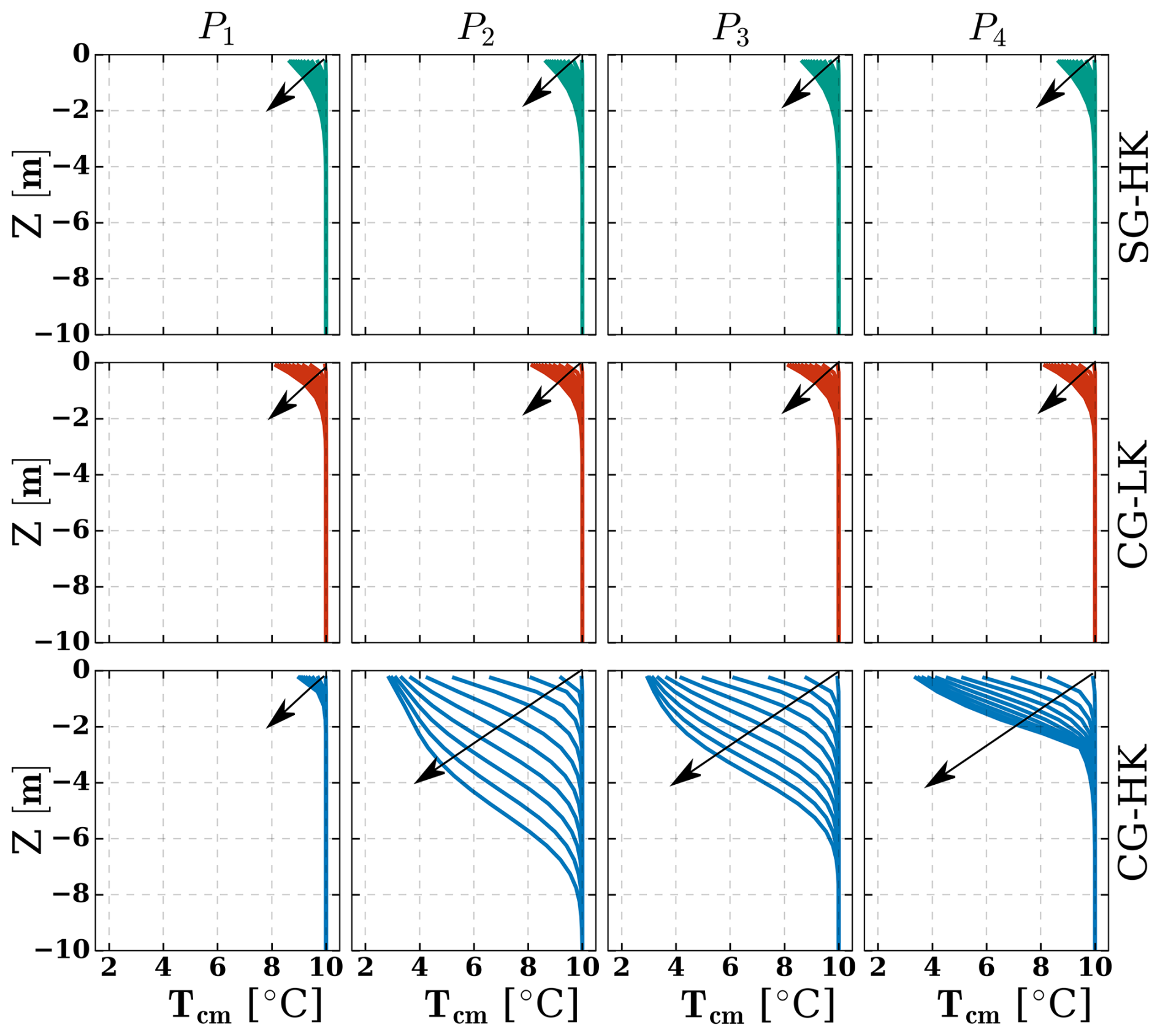
Figure 6 Daily sediment temperature profiles for the winter regime up to 10 d. Arrows indicate time progression from beginning (right) to end (left). Green lines represent the SG-HK case (S-GEOtop with high permeability), red lines represent the CG-LK case (CE-GEOtop with low permeability), and blue lines represent the CG-HK case (CE-GEOtop with high permeability). Profiles at P₁, P₂, P₃, and P₄ correspond to the upper, two middle, and bottom sections of the talus slope (Fig. 5c).

In the SG-HK case, all temperature profiles show similar behaviour due to heat transfer restricted to one-dimensional vertical heat conduction. After 10 d, a slight surface cooling of about 1.5 °C is observed. Similarly, there is a small temperature drop in the CG-LK case, and temperatures are very similar in magnitude to those obtained in the SG-HK case, except they are slightly higher at the surface. The differences between CG-LK and SG-HK at the surface can be attributed to the different thermal conductivity calculations, with SG-HK overestimating the thermal conductivity of dry sediments (as outlined in Sect. 2.3.2). Conversely, the CG-HK case, which considers coarse sediments, displays distinctive differences among the four profiles. The upper section (P₁) exhibits higher temperatures, while a more pronounced cooling is evident in the middle (P₂ and P₃) and bottom (P₄) sections. The middle section cools by 7 °C and the bottom section by 6.5 °C, with lower temperatures penetrating to depths of 4–6 m.

In the CG-HK case, the airflow streamlines indicate that the temperature distributions are influenced by natural convection (Fig. 7). Initially, cold air infiltrates mainly at the bottom of the talus slope, pushing out warmer air at the top, leading to the most substantial temperature drop in the lower section (Fig. 7a). As the simulation progresses, the primary infiltration area shifts to the middle, forming a V-shaped pattern in the streamlines. The perpendicular nature of the air infiltration in this section allows for the cold front to penetrate deeper into the slope. This flow pattern correlates with the talus slope's geometry, where the middle part, having the highest Rayleigh number (Eq. 1), exhibits the greatest potential for natural convection and airflow. These results align with previous studies on talus slopes (Morard et al., 2008; Popescu et al., 2017), indicating that cold air enters the middle–bottom section and warm air rises to the top. This explains the temperature distribution in Fig. 6, where cold-air infiltration decreases temperatures in the middle–bottom section, while warmer air maintains a stable temperature in the top section.

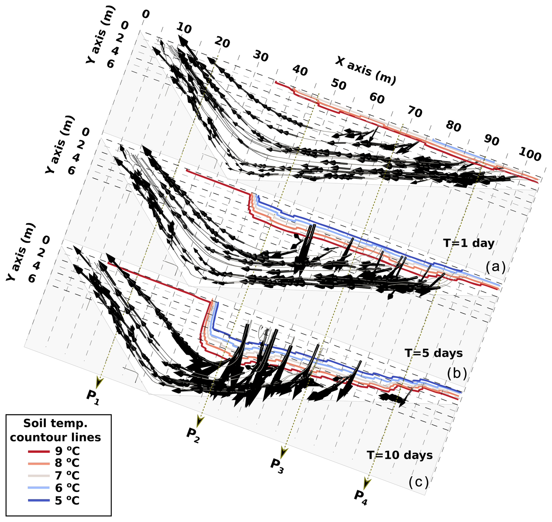
Figure 7 Airflow streamlines in the talus slope for the case CG-HK during the winter phase after 1, 5, and 10 d of simulation. The grey lines show the air streamlines, while the arrows represent the direction and relative magnitude of the airflow velocity. The coloured lines represent the sediment temperature contour lines.

4.2.2 Summer regime

To simulate the summer regime, the initial temperature of the talus and bedrock was set to 10 °C, while the external air temperature was set to 17.5 °C. All temperature profiles show similar patterns for the SG-HK case (see Fig. 8), with a surface temperature increase of approximately 1.5 °C after 10 d. The CG-LK case once again demonstrates a lack of natural convection in lower-permeability sediments, leading to temperature profiles similar to those of the SG-HK case. Conversely, the CG-HK scenario predicts a slight temperature increase at the bottom section surface and a stronger increase at the top section surface (5 °C). Interestingly, the higher temperatures in the middle top section of the talus for this case suggest that convection creates less favourable conditions for permafrost occurrence.

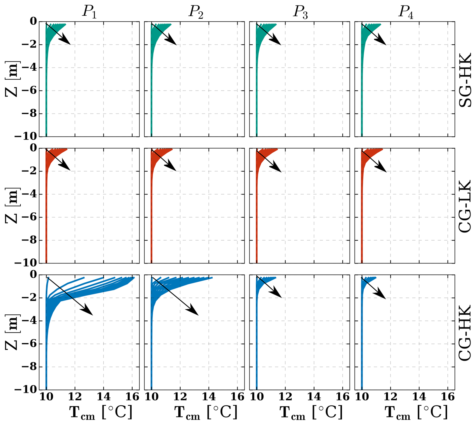
Figure 8 Daily sediment temperature profiles for the summer regime up to 10 d. Arrows indicate time progression from beginning (left) to end (right). Green lines represent the SG-HK case (S-GEOtop with high permeability), red lines represent the CG-LK case (CE-GEOtop with low permeability), and blue lines represent the CG-HK case (CE-GEOtop with high permeability). Profiles at P₁, P₂, P₃, and P₄ correspond to the upper, two middle, and bottom sections of the talus slope (Fig. 5c).

The airflow streamlines for the summer CG-HK case reveal that the temperature distributions are explained by a reversal of the airflow that goes from the top to the bottom of the talus (Fig. 9). This reversal leads to an increase in temperature in the upper section due to warm air infiltration, while the lower zone maintains a temperature of around 10–11 °C throughout the simulation as air flows from within the talus slope. This flow pattern supports the “cold reservoir” observations, where a cooler airflow persists in summer, keeping some middle–lower zones at low temperatures (Popescu et al., 2017; Morard et al., 2008).

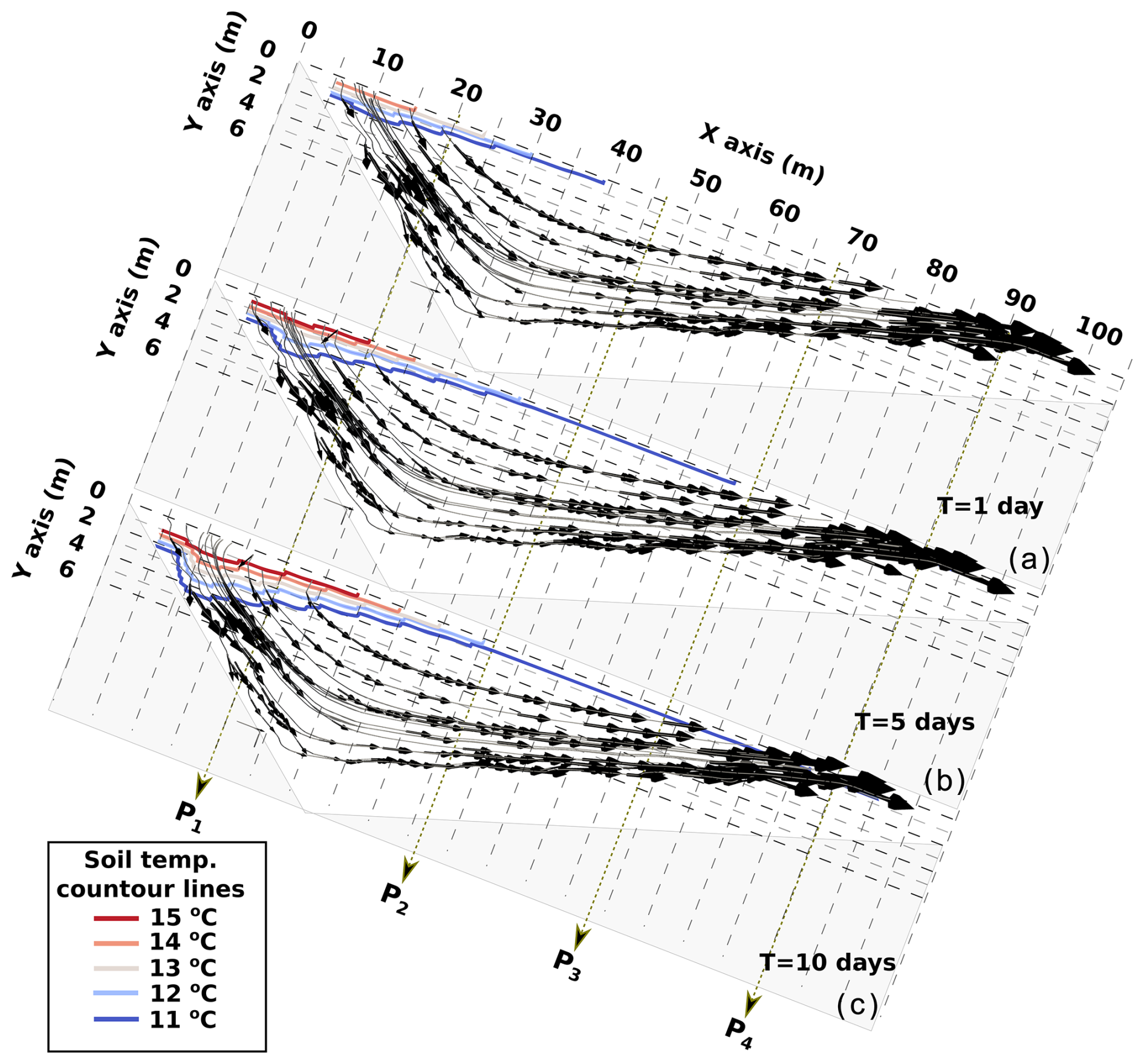
Figure 9 Airflow streamlines in the talus slope for the case CG-HK during the summer phase after 1, 5, and 10 d of simulation. The grey lines show the air streamlines, while the arrows represent the direction and magnitude of the airflow velocity.

4.3 Permafrost predictions

This section elaborates on the CE-GEOtop model's capability to predict permafrost distribution within the Babylon talus slope. The model is forced with half-hourly meteorological data from the nearby (∼0.5 km) Opabin weather station (He and Hayashi, 2019), including precipitation, wind speed and direction, relative humidity, air temperature, incoming longwave radiation, and cloud fraction. Due to the high spatial variability in solar radiation resulting from topographic shading (see Sect. 2.3.4), direct use of measured shortwave radiation is not feasible. Instead, the half-hourly cloud fraction is derived from measured incoming solar radiation (Long et al., 2006) and combined with the hourly sun position and topographic shading to calculate pixel-specific incoming solar radiation across the model domain. The spatial distribution of precipitation, relative humidity, and air temperature was achieved using lapse rates calculated by Hood (2013) from measurements along an elevation transect in the local area.

The model's dimensions, including spatial discretization and the bedrock depth, are consistent with the setup described in the preceding section (Fig. 5c). However, this analysis incorporates distinct sediment permeability and thermal properties. Based on the findings of Kurylyk and Hayashi (2017), a low-conductivity layer ($k=\mathrm{3.75}\times {\mathrm{10}}^{-\mathrm{11}}$ m²) was incorporated in the bottom of the talus sediments. Given that the talus is predominantly composed of cobble- to boulder-sized rocks and lacks fine sediments (Muir et al., 2011), a uniform permeability of $\mathrm{1.5}\times {\mathrm{10}}^{-\mathrm{6}}$ m² (d₁₀=80 mm) was chosen to represent the entire unit, which is likely conservative considering the larger sediments observed in the field. The sediment lithology is assumed to mirror the overlying rockwall, with approximately 65 % quartzite and 35 % limestone (Price et al., 1980). Quartzite possesses thermal conductivity of λ_T=5.7 $\mathrm{W}{\mathrm{m}}^{-\mathrm{1}}{\mathrm{K}}^{-\mathrm{1}}$ (Jones, 2003), while limestone has thermal conductivity of λ_T=2.9 $\mathrm{W}{\mathrm{m}}^{-\mathrm{1}}{\mathrm{K}}^{-\mathrm{1}}$ (Thomas et al., 1973). Additionally, the volumetric heat capacity of limestone (2.1×10⁶ $\mathrm{J}{\mathrm{m}}^{-\mathrm{3}}{\mathrm{K}}^{-\mathrm{1}}$; Shen et al., 2018) is slightly higher than that of quartzite (1.9×10⁶ $\mathrm{J}{\mathrm{m}}^{-\mathrm{3}}{\mathrm{K}}^{-\mathrm{1}}$; Jones, 2003). Consequently, the thermal properties of the talus sediments were calculated proportionally to the quantities of quartzite and limestone.

The presence of snow has a strong effect on sediments' temperature. To verify the accuracy of CE-GEOtop's simulated snow water equivalent (SWE), it was compared to the snow cover evolution estimated by Hood and Hayashi (2015) in the Opabin watershed, which includes the Babylon talus slope. Hood and Hayashi (2015) validated the Utah Energy Balance (UEB) model using extensive field campaigns. The Babylon talus slope falls within the regions covered by oblique-angle terrestrial photography used for UEB model validation, so it is aimed to match the snow cover period rather than the exact SWE values.

The surface aerodynamic roughness was set to 20 mm and the rain threshold temperature to 1 °C in CE-GEOtop (Hood and Hayashi, 2015). While Hood and Hayashi (2015) simulations began in mid-April with measured snow water equivalent (SWE) as the starting condition, CE-GEOtop simulations, driven solely by meteorological data, spanned 2 years to mitigate the uncertainty in initial conditions. Figure 10b compares SWE from CE-GEOtop and UEB. Although there are differences in the magnitude and timing of peak SWE, both models capture similar snow depletion patterns, coinciding in the timing of snow-free ground. This suggests that CE-GEOtop can reasonably reproduce SWE dynamics in the Babylon talus slope, supporting its applicability in permafrost-related studies.

Figure 10 (a) The observed air temperature. The left axis of (b) shows the simulated SWE, where the green line represents the CE-GEOtop simulated SWE, while the red line represents the UEB-simulated SWE. The right axis of (b) shows the total precipitation histogram.

4.3.1 Long-term simulation

The long-term effects of natural convection on sediment temperatures at the Babylon talus slope were examined through multi-year simulations, focusing on an average hydrological year from the period of 2005–2020, where the MAAT was −1.4 °C and the average maximum snow depth was 1.6 m. Consequently, the hydrological year of 2009–2010 was chosen due to its air temperatures and snow depth closely aligning with the period's average (MAAT: −1.3 °C; max snow depth: 1.8 m). A spin-up simulation was performed to establish a stable thermal regime by repeating the meteorological forcings for the 2009–2010 hydrological year across 100 cycles (Ross et al., 2021).

The analysis considered four cases using the same permeability of $k=\mathrm{1.5}\times {\mathrm{10}}^{-\mathrm{6}}$ m²: (i) S-GEOtop (SG), (ii) CE-GEOtop and the air convection module turned off (CG-AO), (iii) CE-GEOtop (CG), and (iv) CE-GEOtop assuming local thermal equilibrium conditions (CG-LTE). Figure 11 shows the sediment temperature profiles for the last day of each month for the last (i.e. 100th) simulated year. For all cases, bedrock is assumed to be almost impermeable with $k=\mathrm{2}\times {\mathrm{10}}^{-\mathrm{15}}$ m² (Hayashi, 2020).

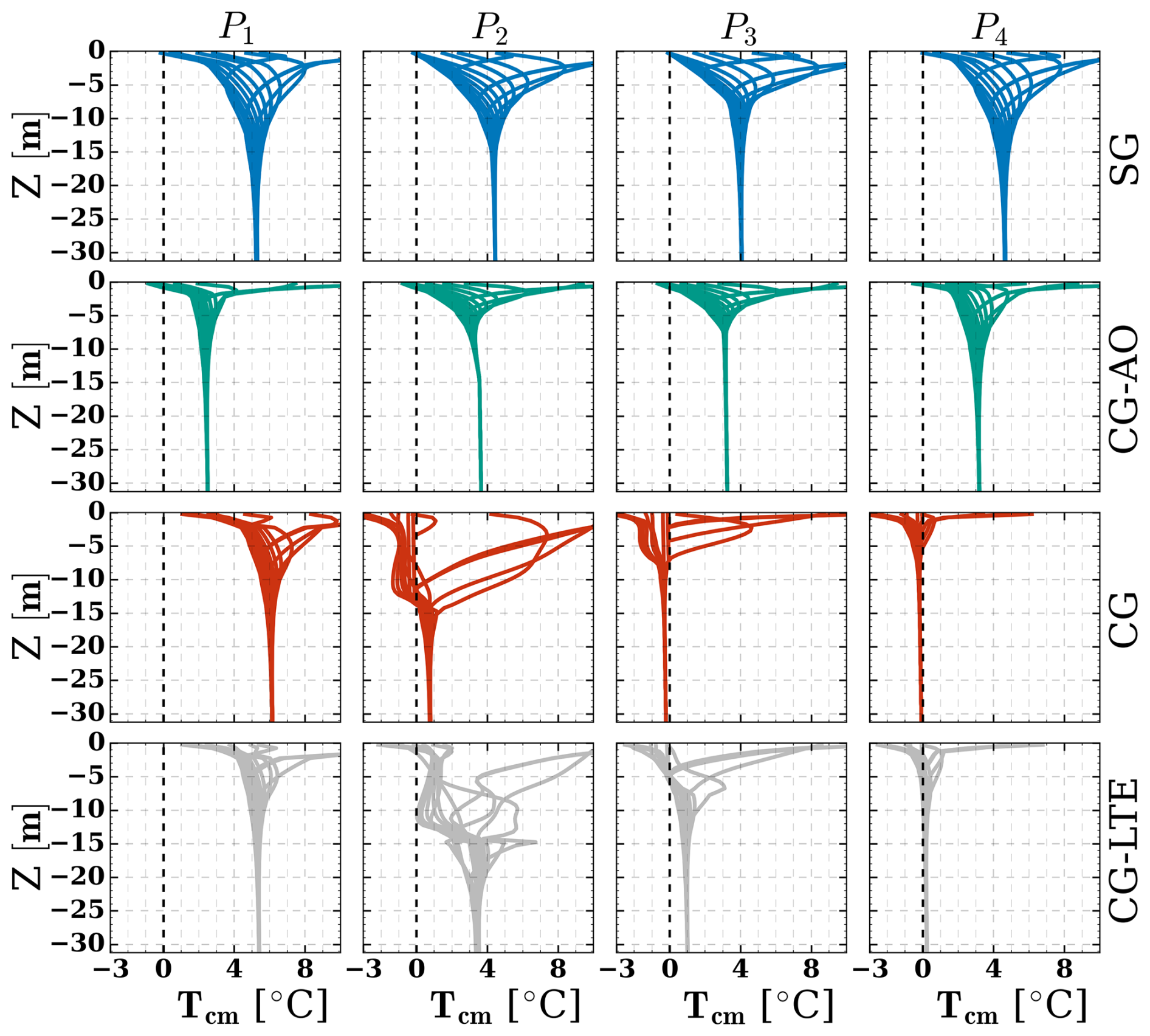
Figure 11 Sediment temperature profiles for the last day of each month for the last simulated year. The blue lines show the temperature profiles for the S-GEOtop case (SG), the green lines show the temperature profiles for the CE-GEOtop case with the air convection module turned off (CG-AO), the red lines show the temperature profiles for the CE-GEOtop case (CG), and the grey lines show the temperature profiles for the CE-GEOtop case assuming LTE (CG-LTE). Profiles at P₁, P₂, P₃, and P₄ correspond to the upper, two middle, and bottom sections of the talus slope (Fig. 5c).

The SG case results indicate no permafrost in the Babylon talus slope, and temperatures remain relatively consistent across all profiles. Surface temperatures drop below freezing for almost half the year, while temperatures at greater depths stabilize around 5 °C. Similarly, the CG-AO results show no indication of permafrost. A comparison of the SG and CG-AO results shows the effect of CE-GEOtop's shadow calculation and thermal conductivity modifications. The modified shadow computations result in lower temperatures in the upper profiles (P₁ and P₂) in the CG-AO case, as the upper zone of the talus is closer to the rockwall, reducing incoming solar radiation. Conversely, the narrower temperature range at greater depths in CG-AO is due to the changes in thermal conductivity estimations, where lower thermal conductivity leads to increased surface temperature gradients but reduces temperature changes with depth. These simulations, when compared with observed permafrost (Fig. 3), suggest that current climate conditions might not sustain permafrost, indicating permafrost thawing and initial formation under cooler climatic conditions.

The CG simulation, however, reveals a different situation and predicts the existence of permafrost at depths ranging from 10 to 35 m in the middle–lower section of the talus slope. Profiles P₁, P₂, and P₃ exhibit similar temperatures, whereas the upper profile P₄ indicates warmer conditions. These results indicate that the current climate conditions are capable of maintaining permafrost, with natural convection playing a critical role in preserving cold temperatures and permafrost in coarse sediments. A comparison of the CG and CG-AO results indicates that natural convection leads to a 3–4 °C reduction in temperatures in the lower profiles (P₃ and P₄).

In the LTE simulation (CG-LTE), temperature profiles closely resemble those from the LTNE simulation (CG) at the extremities of the talus slope (P₁ and P₄). However, differences arise in the midsection (P₂ and P₃), where the LTNE approach indicates lower temperatures between 15–35 m. Conversely, the LTE approach reduces the cooling effect of natural convection and fails to predict permafrost. Natural convection's effectiveness in sediment cooling relies not only on air flux initiation but also on the sinking of colder, denser air, which facilitates energy transfer throughout the sediment profile. This dynamic is overlooked in the LTE approach, where cold air cannot descend, restricting energy transfer from the surface to deeper depths. This phenomenon is evident in the temperature profiles at P₂ and P₃, where both simulations exhibit negative temperatures within the top 5 m of sediment. However, only the LTNE simulation shows deep-reaching cold-temperature effects.

4.4 Permafrost effect on discharges

This section examines the effect of permafrost on spring discharges and temperatures by comparing the results of CG and CG-AO cases. The hydrological year of 2007–2008 was simulated because measured discharge and temperature data of the Babylon basin were available for July–September 2008 (Muir et al., 2011). Figure 12 shows the summer 2008 simulated discharge and spring temperature. Since the GEOtop domain is smaller than the Babylon basin, the discharges are normalized by the area and shown in mm d⁻¹. For profiles P₃ and P₄, sediment temperature, liquid water content, and ice content for four instants during this period are shown in Appendix B (Fig. B1).

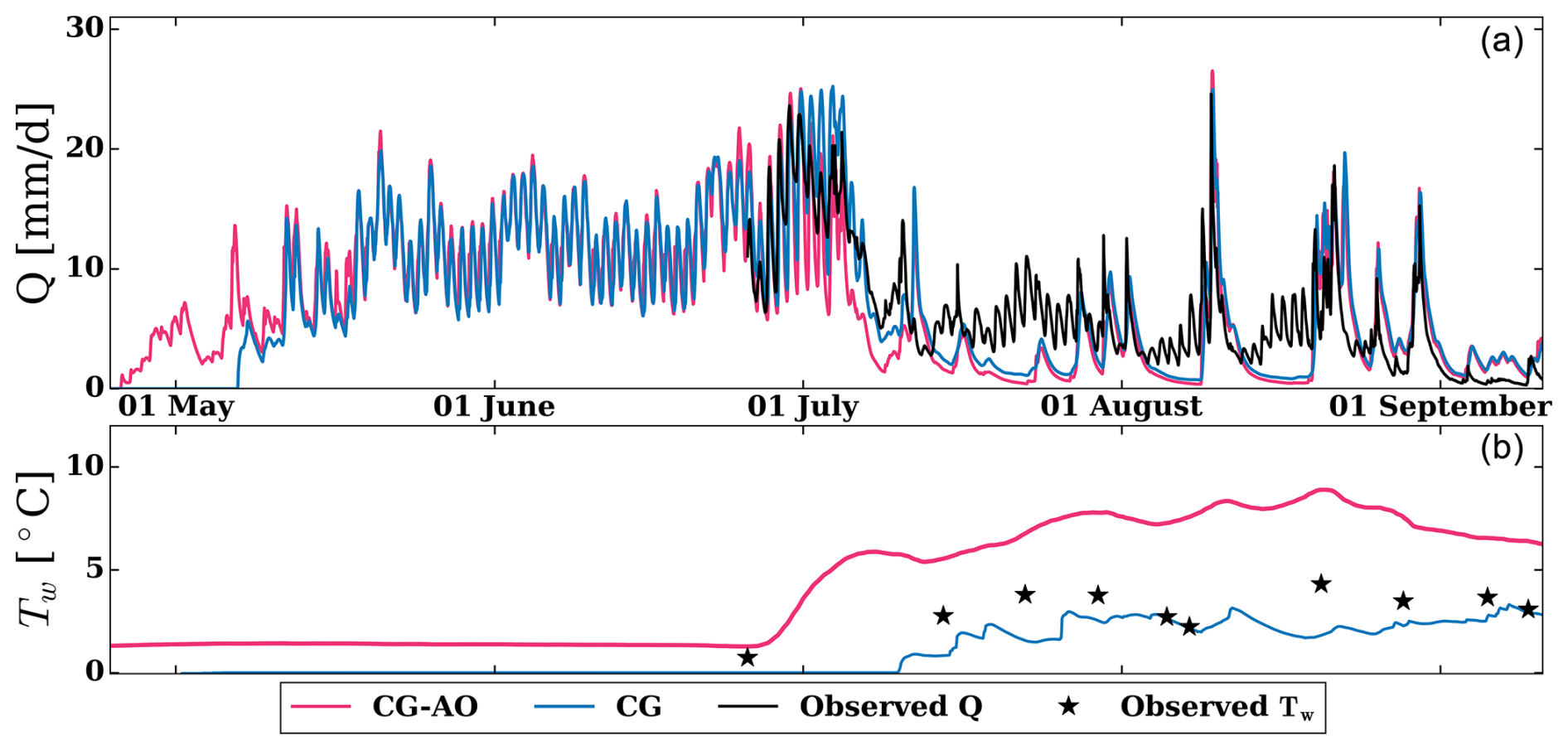
Figure 12 Effects of permafrost on discharge rates and spring water temperatures. (a) Hourly simulated and observed discharges. (b) Hourly simulated and observed temperatures. Pink lines show simulation results from the CE-GEOtop case with the air convection module turned off (CG-AO), while blue lines represent the CE-GEOtop case with air convection enabled (CG). In (a), black lines indicate measured discharge; in (b), black stars indicate measured water temperatures.

The simulations for the scenario involving permafrost (CG) showed that the onset of spring flow occurred approximately 2 weeks later compared to the scenario without permafrost (CG-AO). In early May, the CG case exhibited negative temperatures and low water content throughout the talus, impeding infiltration and groundwater movement. On the other hand, the CG-AO scenario had positive temperatures, enabling groundwater to reach the base of the talus, increasing water content in this area, and resulting in earlier discharge at the model outlet.

These differences are attributable to intra-talus groundwater flow processes. The simulated permafrost within the talus slope is discontinuous and characterized by relatively low ice content, which prevents the formation of a continuous impermeable permafrost layer and consequently precludes supra-permafrost runoff. Thus, the hydrological behaviour is dominated primarily by vertical infiltration through more conductive upper talus layers to deeper, less conductive but more saturated zones near the bedrock.

From mid-May to July, both cases displayed similar behaviour. However, slightly negative temperatures persisted in the middle–lower sections of the talus in the case with permafrost, temporarily delaying groundwater flow by partially freezing and retaining infiltrated water. These conditions explain the subtle differences in discharge observed during May and June. Specifically, in the permafrost scenario (CG), discharge minimums tended to be higher, and the discharge maximums lower, reflecting a more buffered hydrological response to snowmelt and rainfall events. This buffering effect arises from water re-freezing and reduced hydraulic conductivity associated with negative temperatures and higher ice content within profiles P₃ and P₄ during this period.

The Nash–Sutcliffe efficiency (NSE) coefficient was calculated using daily discharge values, yielding an overall NSE of 0.48 for the CG-AO case and 0.55 for the CG case. According to Moriasi et al. (2015), daily NSE values greater than 0.5 are considered satisfactory, indicating that the model incorporating permafrost (CG case) provided a more accurate representation of basin discharge. Particularly, both cases aligned more closely with observed discharge during the last week of June and the first week of July. However, from mid-July onward, contributions from late-lying snowpack in zones not considered in the model became more significant (present in the upper part of the Babylon talus slope as depicted in Fig. 3). As a result, the simulated discharge showed lower magnitudes than the observed values, matching the observed discharges only during precipitation events. Additionally, when comparing the spring temperatures to the measured data, it is evident that the temperatures from the model with permafrost closely resemble the measured values, while the case without permafrost overestimates the spring temperatures. These findings support the idea that the low water temperature during the summer may be related to the presence of coarse sediments and permafrost occurrence.

5 Conclusions

This study improved the GEOtop 3.0 model (S-GEOtop) by incorporating natural convection through the local thermal non-equilibrium (LTNE) approach. The LTNE approach accounts for a different temperature for the air inside the sediment pores with respect to the other phases, including water, ice, and sediments. Additionally, adjustments were made to the thermal conductivity calculations and cast shadows to enhance the energy simulations in alpine landforms. The modified convection-enhanced GEOtop (CE-GEOtop) model was evaluated on a talus slope in the Canadian Rockies with permafrost identification from field data.

Talus slopes with coarse sediments exhibit a thermal anomaly, where the middle–lower sections present lower temperatures than the top of the talus. The CE-GEOtop model successfully captured this phenomenon, depicting an inflow of cold air at the base of the talus slope and warmer air exiting at the top during winter months, as well as a reversal of this flow during summer months. The strength of natural convection is defined by the Darcy–Rayleigh number (Ra). Simulations indicated that flow is initiated when Ra exceeds Ra_c, but larger Ra is necessary for natural convection impacting sediment temperatures. Moreover, on longer timescales, sporadic instances with large Ra are insufficient for inducing cooling, necessitating either recurrent or prolonged periods with elevated temperature gradients.

The simulations showed that air temperature within the sediments rarely reaches local thermal equilibrium with the other phases in the presence of natural convection. As a result, the long-term simulations performed using the local thermal equilibrium approach overestimated temperatures and failed to predict permafrost presence in the talus slope, underscoring the significance of considering thermal non-equilibrium conditions.

The S-GEOtop simulations under current climate conditions also failed to predict permafrost in the talus, but the CE-GEOtop model successfully predicted permafrost from depths of 10–35 m in the middle–bottom section of the slope. This highlights the important role of natural convection in coarse sediments' energy balance and the relevance of using the LTNE approach to represent this process correctly. The presence of permafrost affects the hydrological response of the talus, resulting in delayed discharges after snowmelt and rain due to partial groundwater freezing in the lower layer of the sediments. During summer, persistently cold discharges were simulated when permafrost was present, matching the measured temperatures at the talus outlet. Overall, this study demonstrated the important role of natural convection in permafrost dynamics within alpine landforms, as well as the necessity to consider this physical process in heat transport modelling in cold environments dominated by coarse, blocky sediments.

CE-GEOtop offers comprehensive capabilities to simulate snow cover, ground temperatures, permafrost, and water budgets, providing a new framework to analyze the interplay between groundwater discharge and permafrost, as well as the effects of surficial geology on temperature distribution. Future research should address the interplay between air temperatures, snow depth, and natural convection under a warmer climate, particularly to forecast sediment temperature, permafrost extent, and groundwater discharges. Additionally, further examination of the effect of surficial geology on permafrost distribution and natural convection is necessary, with particular attention given to the role of spatial heterogeneities in permeability, deposit depth, and bedrock configuration. All these factors strongly influence the strength of natural convection and the patterns of airflow within the sediments.

Appendix A: Governing equations

A1 Numerical implementation

The four main equations are solved in a time-lagged manner, in the following order: (i) air mass balance (Eq. 5), (ii) air energy balance (Eq. 8), (iii) composite-medium energy balance (Eq. 4), and (iv) water mass balance (Eq. 3). These equations can be generalized using the following form:

$$\begin{array}{}\text{(A1)}& {\displaystyle }{\displaystyle \frac{\partial F\left(\mathit{\chi }\right)}{\partial t}}+\mathrm{\nabla }\cdot (-L(\mathit{\chi }\left)\mathrm{\nabla }\mathit{\chi }\right)+S=\mathrm{0}.\end{array}$$

Here, χ represents the unknown variable function of space and time, F is a non-linear function, S is the sink term, and L is a property dependent on χ. By integrating this equation over a control volume V_c and using an implicit approach, we obtain

$$\begin{array}{}\text{(A2)}& \begin{array}{rl}& {\displaystyle \frac{\left(F\left({\mathit{\chi }}_i^{n+\mathrm{1}}\right)-F\left({\mathit{\chi }}_i^n\right)\right)\mathrm{\Omega }\mathrm{\Delta }z}{\mathrm{\Delta }t}}-\sum _j^M{\displaystyle \frac{L_{ij}^{n+\mathrm{1}}{\mathrm{\Omega }}_{ij}}{D_{ij}}}\left({\mathit{\chi }}_j^{n+\mathrm{1}}-{\mathit{\chi }}_i^{n+\mathrm{1}}\right)\\ & +S_{\mathrm{w}}\mathrm{\Omega }\mathrm{\Delta }z=G_{il}\left({\mathit{\chi }}^{n+\mathrm{1}}\right)\approx \mathrm{0}.\end{array}\end{array}$$

This equation is written for the generic ith cell, where n represents the previous time step at which the solution is known and n+1 is the next time step at which the solution is unknown. Δt is the time step, j is the index of the m adjacent cells with which the ith cell can exchange fluxes, L_ij represents the conductivity between cell i and j, D_ij denotes the distance between the centers of cells i and j, S_w represents the sink terms, and G_i is the residual to be minimized to find a solution. As explained in Endrizzi et al. (2014), Eq. (A2) is solved using the Newton–Raphson method.

A2 Mass balance

The governing coupled equation for two-phase flow is the following (Nield and Bejan, 2017):

$$\begin{array}{ll}{\displaystyle }& {\displaystyle \frac{\partial ({\mathit{\rho }}_{\mathrm{w}}{\mathit{\theta }}_{\mathrm{w}}+{\mathit{\rho }}_{\mathrm{i}}{\mathit{\theta }}_{\mathrm{i}})}{\partial t}}+{\displaystyle \frac{\partial {\mathit{\rho }}_{\mathrm{a}}{\mathit{\theta }}_{\mathrm{a}}}{\partial t}}+{\mathit{\rho }}_{\mathrm{w}}\mathrm{\nabla }\cdot \left({\mathit{J}}_{\mathrm{w}}\right)+{\mathit{\rho }}_{\mathrm{a}}\mathrm{\nabla }\cdot \left({\mathit{J}}_{\mathrm{a}}\right)\\ \text{(A3)}& {\displaystyle }& {\displaystyle }+S_g+S_{\mathrm{w}}=\mathrm{0}.\end{array}$$

To solve this system, we will not consider the interplay between the fluxes of water and air. This means that the movement of water will not cause air movement and air movement will not cause water movement. With this assumption, we can separate Eq. (A3) using the split method, getting

$$\begin{array}{}\text{(A4)}& {\displaystyle }& {\displaystyle \frac{\partial ({\mathit{\rho }}_{\mathrm{w}}{\mathit{\theta }}_{\mathrm{w}}+{\mathit{\rho }}_{\mathrm{i}}{\mathit{\theta }}_{\mathrm{i}})}{\partial t}}+{\mathit{\rho }}_{\mathrm{w}}\mathrm{\nabla }\cdot \left({\mathit{J}}_{\mathrm{w}}\right)+S_{\mathrm{w}}=\mathrm{0},\text{(A5)}& {\displaystyle }& {\displaystyle \frac{\partial \left({\mathit{\rho }}_{\mathrm{a}}{\mathit{\theta }}_{\mathrm{a}}\right)}{\partial t}}+{\mathit{\rho }}_{\mathrm{a}}\mathrm{\nabla }\cdot \left({\mathit{J}}_{\mathrm{a}}\right)+S_{\mathrm{a}}=\mathrm{0}.\end{array}$$

Equation (A4) is used to solve the water flow and Eq. (A5) to solve the airflow. Using the Oberbeck–Boussinesq approximation to solve the airflow, the air density (ρ_a) can go out of the partial time derivative. The air content in a control volume can only change if there is a change in water or ice content ($\partial {\mathit{\theta }}_{\mathrm{a}}=-\partial {\mathit{\theta }}_{\mathrm{w}}-\partial {\mathit{\theta }}_{\mathrm{i}}$), but since we neglected the interplay between the fluxes of water and air, we get $\frac{\partial \left({\mathit{\theta }}_{\mathrm{a}}\right)}{\partial t}\sim \mathrm{0}$. This assumption is valid as, in this case, temperature gradients dominate the air fluxes, rather than air fluxes being induced by water movement. Since moisture in the air has a minimal effect on air density at temperatures below 20 °C, this formulation also neglects the effect of moisture on air density. Thus, the airflow equation reduces to

$$\begin{array}{}\text{(A6)}& {\displaystyle }{\displaystyle }{\mathit{\rho }}_{\mathrm{a}}\mathrm{\nabla }\cdot \left({\mathit{J}}_{\mathrm{a}}\right)+S_g=\mathrm{0}.\end{array}$$

This equation is integrated over a volume V_c, and considering that $J_{\mathrm{a}}=-\frac{k_{\text{ra}}k}{{\mathit{\mu }}_{\mathrm{a}}}(\mathrm{\nabla }P-{\mathit{\rho }}_{\mathrm{a}}\mathit{g})$, this yields

$$\begin{array}{ll}{\displaystyle }& {\displaystyle }-\sum _j^M{\displaystyle \frac{k_{ij\mathrm{a}}^{n+\mathrm{1}}{\mathrm{\Omega }}_{ij}}{D_{ij}}}\left(P_{jg}^{n+\mathrm{1}}-P_{i\mathrm{a}}^{n+\mathrm{1}}\right)\\ {\displaystyle }& {\displaystyle }-{\displaystyle \frac{K_{ij\mathrm{a}}^{n+\mathrm{1}}{\mathrm{\Omega }}_{ij}}{D_{ij}}}{\text{Tb}}_{i\mathrm{a}}^{n+\mathrm{1}}(z_{jg}-z_{i\mathrm{a}}){|}_{\text{top}}\\ {\displaystyle }& {\displaystyle }-{\displaystyle \frac{K_{ij\mathrm{a}}^{n+\mathrm{1}}{\mathrm{\Omega }}_{ij}}{D_{ij}}}{\text{Tb}}_{i\mathrm{a}}^{n+\mathrm{1}}(z_{jg}-z_{i\mathrm{a}}){|}_{\text{bottom}}\\ \text{(A7)}& {\displaystyle }& {\displaystyle }+S_g\mathrm{\Omega }\mathrm{\Delta }z=G_{i\mathrm{a}}\left(P_{i\mathrm{a}}^{n+\mathrm{1}}\right)\sim \mathrm{0}.\end{array}$$

${\text{Tb}}_i^{n+\mathrm{1}}={\mathit{\rho }}_{\mathrm{r}g}g(\mathrm{1}-\mathit{\beta }(T_{i\mathrm{a}}^{n+\mathrm{1}}-T_{\text{ref}}\left)\right)$ represents the buoyancy term and $K_{\mathrm{a}}=\frac{k_{\text{ra}}k}{{\mathit{\mu }}_{\mathrm{a}}}$ the air conductivity.

A3 Energy balance

The heat transport equation to solve for the air energy balance is presented in Eq. (8). Similarly, as before, this equation is integrated over a volume V_c:

$$\begin{array}{ll}{\displaystyle }& {\displaystyle \frac{\mathrm{\Delta }z{\mathit{\rho }}_{\mathrm{a}}{C}_{\mathrm{a}}\mathrm{\Omega }}{\mathrm{\Delta }t}}\left({\mathit{\theta }}_{i\mathrm{a}}^{n+\mathrm{1}}\left(T_{i\mathrm{a}}^{n+\mathrm{1}}-T_{i\mathrm{a}}^n\right)\right)\\ {\displaystyle }& {\displaystyle }-\sum _j^M{\displaystyle \frac{{\mathit{\theta }}_{gij}{\mathit{\lambda }}_g{\mathrm{\Omega }}_{ij}}{D_{ij}}}\left(T_{jg}^{n+\mathrm{1}}-T_{i\mathrm{a}}^{n+\mathrm{1}}\right)\\ {\displaystyle }& {\displaystyle }+\sum _j^M\left({\mathit{J}}_{ijg}^n{\mathrm{\Omega }}_{ij}{\mathit{\rho }}_{\mathrm{a}}{C}_{\mathrm{a}}\left(T_{ijg}^{n+\mathrm{1}}-T_{\text{ref}}\right)\right){|}_{\text{face}}\\ {\displaystyle }& {\displaystyle }+\mathrm{\Delta }z\mathrm{\Omega }h{T}_{i\mathrm{a}}^{n+\mathrm{1}}-\mathrm{\Delta }z\mathrm{\Omega }h{T}_{\text{icm}}^{n+\mathrm{1}}\\ \text{(A8)}& {\displaystyle }& {\displaystyle }+S_g\mathrm{\Omega }\mathrm{\Delta }z=R{G}_{i\mathrm{a}}\left(T_{i\mathrm{a}}^{n+\mathrm{1}}\right)\sim \mathrm{0}.\end{array}$$

Appendix B: Additional figure

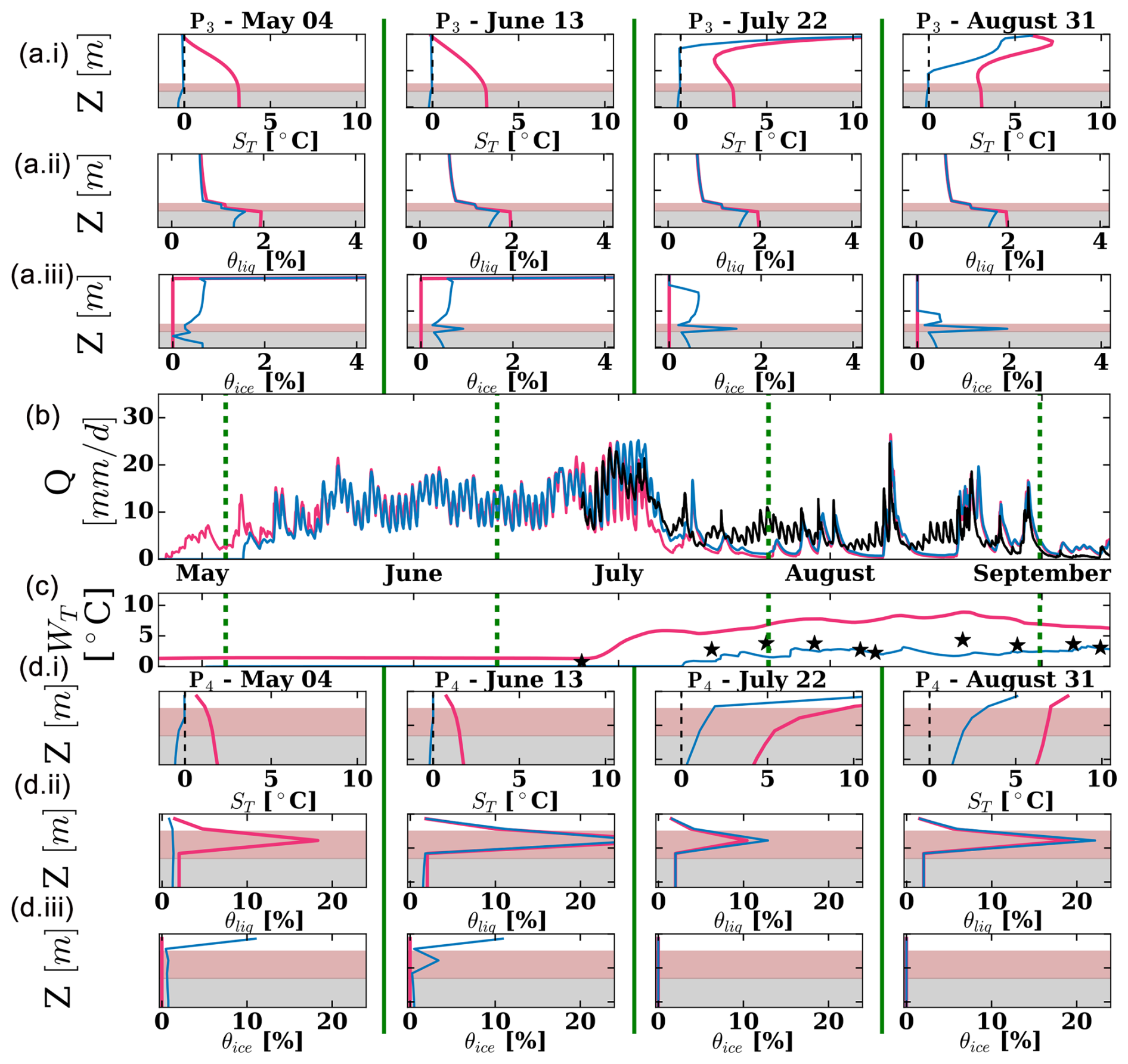
Figure B1 Effects of permafrost on discharge rates and spring water temperatures. Blue lines represent the results for the CG case, while pink lines correspond to the CG-AO case. (a.i–a.iii) The simulated sediment temperatures (S_T), liquid water content (θ_liq), and ice content (θ_ice), respectively, for profile P₃ at four distinct times during the summer of 2008. In these panels, the fine sediment layer is indicated with a brown colour and the bedrock is indicated with a grey colour. (b) The simulated discharges compared with the observed discharges (represented by the black line). (c) The simulated temperatures contrasted with the observed temperatures (indicated by black stars). The dashed vertical green lines in (b) and (c) indicate the four distinct times where the profiles P₃ and P₄ are shown. (d.i–d.iii) The simulated sediment temperatures (S_T), liquid water content (θ_liq), and ice content (θ_ice), respectively, for profile P₄ at four distinct times during the summer of 2008. In these panels, the fine sediment layer is indicated with a brown colour and the bedrock is indicated with a grey colour.