Analyzing vegetation effects on snow depth variability in Alaska's boreal forests with airborne lidar

Lidar-derived snow depth and canopy height maps were used to analyze snow depth spatial variability at a boreal forest site in Alaska. High-resolution (0.5 m) airborne lidar data were acquired during NASA's SnowEx Alaska field campaigns during peak snow-on accumulation (March 2022) and snow-off (May 2022). The impact of canopy height on snow distribution was studied at the Caribou Poker Creeks Research Watershed, located northeast of Fairbanks, Alaska, US. Ground-based snow depth measurements were collected concurrently with the March snow-on lidar survey and were compared to collocated lidar-derived snow depths. The comparison between ground-based and lidar-derived snow depths produced a bias of 2.0 cm and a root mean square error (RMSE) of 12.0 cm. The lidar snow depth map showed a mean snow depth of $\stackrel{\mathrm{‾}}{HS}=\mathrm{98}$ cm and a standard deviation of SD=15 cm for the study site. The influence of vegetation on end-of-winter snow depth distribution was analyzed using three canopy height classes: (1) forest, (2) shrub and short stature trees (SSS), and (3) treeless. Results showed a statistically significant difference in median snow depths across canopy height classes, with the largest significant differences between forest and treeless (12–14 cm) and between forest and SSS (8–14 cm). These differences in snow depth correspond to a snow water equivalent range of approximately 20–30 mm. This study provides insights into the spatial variability of snow depths in Alaska's boreal forests by using ground-based measurements to evaluate the accuracy of airborne lidar to estimate snow depths in a boreal forest ecosystem. The results of this research can be used to assist water and resource managers in determining best practices for estimating snow depth and its spatial variability in the boreal forest of Alaska.

1 Introduction

Snow plays a significant role in hydrologic, atmospheric, and ecological processes globally. Snow cover impacts the thermal regime of the soil, water and energy balances, land use decisions, winter recreation, and the timing and volume of spring runoff (Barnett et al., 2005; Boelman et al., 2019; Chapin et al., 2000, 2005). In the boreal forest seasonal snowpack and its melting dominate annual hydrological and climatic patterns (Barnett et al., 2004; Kane and Yang, 2004; Kozii et al., 2017). The snowpack accumulates from the fall through the following spring with few melt or runoff events. The spring snowmelt is often the major hydrological event each year and usually correlates with the peak discharge of the season (Kane and Yang, 2004; Kozii et al., 2017; Tennant et al., 2017).

In boreal forest regions, the spatial and temporal variability of snow depth (HS) can be significant due to static controls such as land cover, topography, soil, and permafrost (Cho et al., 2021; Pastick et al., 2015; Woo, 2012) and due to dynamic processes including canopy–snow interactions (Hojatimalekshah et al., 2021; Kozii et al., 2017; Uhlmann et al., 2018), wind distribution (Homan and Kane, 2015; Liston and Sturm, 1998), longwave and shortwave radiation (Lundquist et al., 2013), and solid and liquid precipitation trends (Bolton et al., 2004; Brown and Goodison, 1996; Kane and Yang, 2004; Lader et al., 2020). Boreal forest snow is classified as cold with thin to moderate (0.3–1.3 m) snow depths and low-density (217 kg m⁻³) snow cover (Sturm and Liston, 2021). The low density is due to the extensive depth hoar (occupying $\mathrm{2}/\mathrm{3}$ to virtually all the snow cover) and few to no melt events during the winter season. New and recent snow layers at the surface of the snow retain their basic snow crystal structures for days due to the cold air temperatures, relatively low amounts of precipitation, and the absence of wind (Sturm and Liston, 2021).

The boreal forest is one of the world's largest forest biomes, making up approximately 30 % of the world's forested regions (Askne et al., 2017). In the Northern Hemisphere, 20 % of the seasonal snow cover occurs within forested regions (Güntner et al., 2007). Forests canopies modify snow accumulation, ablation rates, and overall snow storage by intercepting snowfall (Dickerson-Lange et al., 2021; Lundquist et al., 2013; Storck et al., 2002; Uhlmann et al., 2018). Intercepted snow can account for as much as 40 %–60 % of annual snowfall in boreal forests (Kozii et al., 2017; Pomeroy et al., 2002). All these processes are strongly controlled by the structure of the forest canopy at small spatial scales that interact to create variable snow distribution patterns (Broxton et al., 2015, 2019; Dickerson-Lange et al., 2021; Mazzotti et al., 2019). In boreal regions land cover is a mixture of spruce, deciduous, and mixed forests, shrublands, and low-lying herbaceous wetlands. Snow depth can be noticeably different across land cover types under the same climatic conditions. Accurately accounting for forest effects on snow storage and distribution will become even more important as forests change due to warming climate conditions, forest disturbances, wildfires, insect infestation, and permafrost degradation (Panda et al., 2010; Smith et al., 2021). In turn, these changing forests impact hydrological regimes, water availability, timing and magnitude of snowmelt runoff, and water resources for land and civilian uses (Dickerson-Lange et al., 2021; Hopkinson et al., 2004; Mazzotti et al., 2019; Webb et al., 2020).

Monitoring forest changes and subsequent snow storage and distribution effects is vitally important to water and resource managers. Remote sensing techniques are advancing our understanding of links between forest snow distribution and canopy structure by providing high-resolution spatial data on snow on the ground and the detailed structure of forest canopies at landscape scales and across previously unavailable extends (Harpold et al., 2014; Jacobs et al., 2021; Li et al., 2021). One remote sensing technique, airborne-based light detection and ranging (lidar), has been used for almost two decades to describe snow depths in forests (Hopkinson et al., 2004), and lidar techniques are evolving to better characterize forest properties (land cover, canopy density, height, gaps, etc.) relevant to snow distribution (Li et al., 2021; Mazzotti et al., 2019; Moeser et al., 2016; Tennant et al., 2017; Yang et al., 2018; Zheng et al., 2016). Studies show that, compared to traditional manual measurements, lidar data that provide spatially continuous, high-resolution snow depth maps have greatly advanced the capacity to characterize the spatial variability in snow depth at a mesoscale, i.e., watershed scale (Deems et al., 2013; Harder et al., 2020; Hopkinson et al., 2004, 2012; Jacobs et al., 2021; Nolan et al., 2015; Painter et al., 2016; Trujillo et al., 2007), while maintaining a statistically significant relationship between lidar-derived snow depths and manual field measurements (Douglas and Zhang, 2021; Harpold et al., 2014; Hopkinson et al., 2004, 2012; Jacobs et al., 2021; Mazzotti et al., 2019; Reutebuch et al., 2003). However, when comparing lidar accuracy between forest and non-forested areas, existing validation studies yield contrasting conclusions (Harpold et al., 2014). Despite considerable literature on airborne lidar snow depth retrievals in forested environments, little research has been published on its ability to measure snow depth in boreal forests, and results are varied in identifying what vegetation characteristics are driving snow depth variability in boreal forest ecosystems.

The purpose of this paper is to contribute to limited boreal forest snow remote sensing research by analyzing ground-based snow depth measurements and airborne lidar data to improve snow depth estimation at a watershed scale. Specifically, we ask the following. (1) Can combining ground-based measurements with airborne lidar improve snow depth estimation in the Caribou Poker Creeks Research Watershed (CPCRW)? (2) How does vegetation height influence snow depth variability within CPCRW? Two new airborne lidar-derived data products obtained during the NASA SnowEx Alaska campaigns are used for the analysis. A lidar-derived snow depth map is compared to ground-based measurements to evaluate the accuracy of lidar to estimate snow depths in an Alaska boreal forest. A lidar-derived canopy height map is used to evaluate a vegetation metric that quantifies the spatial variability of snow depths in boreal forests. The results can then be used to educate and assist water and resource managers in the effectiveness of airborne lidar to accurately estimate snow depth and snow water equivalent (SWE) in boreal forests of Alaska. The utility of the lidar-derived vegetation metric can further enhance understanding of vegetation and snow interactions while improving snow modeling applications.

2 Study site and data

2.1 Study site

The study was conducted in the Caribou Poker Creeks Research Watershed located approximately 48 km northwest of Fairbanks, Alaska (Fig. 1). CPCRW is a relatively pristine, 104 km² basin reserved for meteorologic, hydrologic, and ecologic research. The site was established in 1987 as part of the National Science Foundation's Long Term Ecological Research (LTER) Program, and it is one of only two designated forest research facilities in the true boreal forest zone of the United States (USDA Forest Service Pacific Northwest Research Station, 2023). The watershed spans an elevation of 200–830 m and reports a mean annual air temperature of −3.3 °C and mean annual precipitation of 625 mm (USDA Natural Resources Conservation Service), 40 % of which can be snowfall (Liston and Hiemstra, 2011; USDA Forest Service Pacific Northwest Research Station, 2023). Approximately 30 % of its area is underlain by continuous and discontinuous permafrost (Fig. 1) (Bonanza Creek LTER; Haugen et al., 1982).

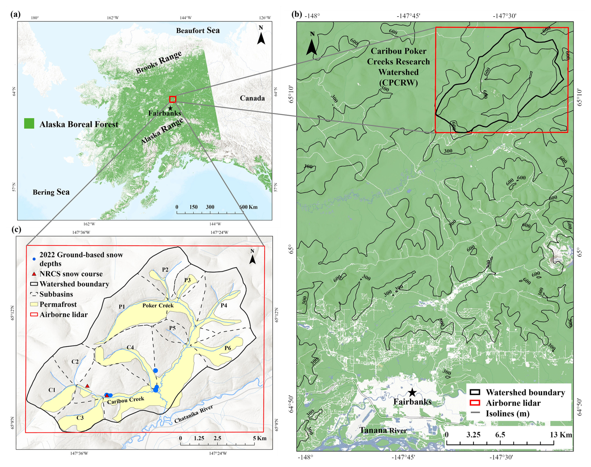
Figure 1 Map of the Alaska boreal forest ecozone (a) and the location of the Caribou Poker Creeks Research Watershed (b). Subbasins of the CPCRW, permafrost areas, the location of ground-based snow depth measurements taken on 11 March 2022, and the coverage of the lidar flight flown on 11 March 2022 are shown on the map in panel (c). Base map source: ESRI.

Two streams are found within CPCRW, Caribou Creek and Poker Creek. The Caribou Creek watershed is divided into four subbasins (C1, C2, C3, and C4), and the Poker Creek watershed is divided into six subbasins (P1, P2, P3, P4, P5, and P6) (Fig. 1) (Haugen et al., 1982). The drainage pattern of the two streams is dendritic, and stream channels in the subdrainages are generally steep-walled and narrow, while the main channels are wider, often with alternating pools and riffles (Bredthauer and Hoch, 1979). The two streams converge at the south-central portion of the watershed and then flow into the Chatanika River. The Chatanika joins the Tolovana River, which flows into the Tanana River and then into the Yukon River. The vegetative cover within the watershed consists of deciduous, evergreen and mixed forests, shrublands, and woody wetlands. A dense understory persists throughout the watershed. South-facing slopes are dominated by well-drained deciduous and mixed forests of aspen (Populus tremuloides), poplar (Populus balsamifera), birch (Betula neoalaskana), and white spruce (Picea glauca). The understory consists of patchy alder (Alnus viridis) and willow (Salix spp.). North-facing slopes are dominated by evergreen forests with black spruce (Picea mariana) as the dominant species. Understories contain dwarf shrubs (e.g., Betula nana, Salix spp., Ledum groenlandicum), feather moss, and lichen (Bonanza Creek LTER, 2023).

2.2 Data

2.2.1 Ground-based snow depths

Ground-based snow depths were obtained from snow measurements conducted in the CPCRW on 11 March 2022 (May et al., 2024) during the planning phase for the NASA SnowEx Alaska campaigns. SnowEx was a multiyear program initiated and funded by the NASA Terrestrial Hydrology Program. Using fieldwork and various remote sensing technologies, SnowEx Alaska aims to determine (Vuyovich et al., 2024) the answer to the following question: how well can we characterize the spatial variability of snow depth and density needed for accurate SWE estimates in the boreal forest by measuring snow depth, density, and vegetation characteristics? In 2022 and 2023, the NASA SnowEx campaigns focused on the Arctic tundra and boreal forest regions of Alaska.

A total of 2114 ground-based snow depth measurements were collected at the study site in a spiral pattern, approximately 1–3 m apart, with a GPS-enabled snow depth measurement device called a magnaprobe (Sturm and Holmgren, 2018). The magnaprobe consists of a 1.3 m long ∼ 1 cm diameter rod with a moveable basket that uses a GPS and a magneto restrictive material inside the rod to record snow depth and location in seconds (Sturm and Holmgren, 2018). GPS horizontal location accuracy is ±2.5 m in open areas but may decrease to 10–15 m in dense forest (Douglas and Zhang, 2021; Sturm and Holmgren, 2018). Snow depth measurements were taken at four sample locations within the CPCRW (Fig. 1); measurements were used as validation points to determine the accuracy of the lidar-derived snow depth map.

Two additional snow depth measurements were obtained from snow course sites operated by the USDA Natural Resources Conservation Service (NRCS) within CPCRW (Fig. 1). Snow depth records date back to December 1969 at both sites, with the 30-year (1991–2020) median snow depths available for the start of each month. At the start of March, the 30-year median snow depth for the Caribou Creek snow course was 58 cm and for the Caribou Snow Pillow snow course was 56 cm (USDA Natural Resources Conservation Service, 2022). Snow depths recorded on 1 March 2022 from the Caribou Creek and Caribou Snow Pillow snow course sites were compared to the SnowEx Alaska ground-based and lidar-derived snow depth values collected on 11 March 2022.

2.2.2 Airborne lidar

Airborne lidar, an active remote sensing system, records the time required for emitted light to travel to the ground and back to an airplane-mounted sensor. The sensor includes a GPS that identifies the X,Y, and Z location of the light energy and an internal measurement unit that provides the orientation of the plane in the sky. The resultant data can be used to create a high-resolution digital terrain model (DTM) that approximates a bare earth surface. Differencing a snow-free from a snow-on surface elevation data set allows for a straightforward mapping of snow depth. In addition to providing spatial data on snow distribution, airborne lidar can produce spatial data on canopy heights by subtracting a bare earth digital terrain model from a digital surface model (DSM). A DSM models the canopy and the top of the vegetation by accounting for all the first, or only, lidar pulses returned to the sensor.

Two airborne lidar surveys were flown over CPCRW (Larsen, 2024). The first was flown prior to the onset of snowmelt on 11 March 2022. The second was flown on 29 May 2022 during snow-free conditions. The lidar flight area of coverage is represented by the red box in Fig. 1 and constitutes the study site. All references to CPCRW and all statistical analysis performed in this study are in reference to the larger area within the lidar box, not the boundary of the watershed (Fig. 1). The 11 March 2022 lidar survey occurred concurrently with ground-based snow depth measurements taken on the same day. Differencing the May snow-free DSM from the May snow-free DTM produced a lidar-derived canopy height map.

The lidar and stereophotogrammetry instruments are combined on a rigid mount and deployed simultaneously in a Cessna T206 aircraft. The lidar scanner uses a 1064 nm wavelength laser and has adjustable pulse repetition frequency up to 2000 kHz. The scanner has a rotating mirror that sweeps the beam across 75° (±37.5° off nadir), resulting in shot lines perpendicular to the flight path (MacGregor et al., 2021). Flight lines are planned with >50 % sidelap to target 20 points per square meter for each survey coverage. The higher pulse frequency and point rate increase the probability of sufficient laser points penetrating the canopy, reaching the ground, and returning to the sensor (Campbell et al., 2018; Deems et al., 2013). The vertical and horizontal accuracy of the lidar snow depth and canopy height maps is ±5.0 cm.

3 Methods

3.1 Lidar data review

The lidar data products were reviewed for quality control and visually inspected for abnormalities. Lidar snow depth and canopy height pixel values that represented unlikely snow depths or canopy heights for the CPCRW, or that displayed abnormal distribution patterns, were removed from the analysis. Negative pixel values, which are usually the result of error points in one of the lidar data sets, were assigned a “no data” code during quality control.

The lidar snow depth map contained pixel values ranging from −300 to 499 cm, an implausible range in snow depths for CPCRW. We referenced the maximum ground-based SnowEx snow depths, the maximum NRCS snow course measurements, and a histogram of the lidar snow depths to determine a plausible snow depth range for CPCRW. A color scale map of the lidar snow depths was generated to identify potential patterns indicating the presence of unlikely snow depth values. The lidar snow depth map was then corrected to include only pixels occurring within the plausible snow depth range, and all remaining pixels were classified as “no data.”

The lidar canopy height map contained pixel values ranging from −3 to 40 m. All positive canopy height values were included in the analysis and classified according to the vegetation found within CPCRW. Canopy height classes were determined after referencing the vegetation classification used in the US Geological Survey National Land Cover Database (NLCD) 2016 Land Cover – Alaska (ver. 2.0, July 2020) (Dewitz, 2019) and the Fuel Model Guide to Alaska Vegetation (Alaska Fuel Model Guide Task Group, 2018).

3.2 Collocated ground-based and lidar-derived snow depths

Ground-based measurements were used as validation points to evaluate the accuracy of the lidar-derived snow depth map. GPS coordinates for every ground-based snow depth measurement were extracted from the magnaprobe data logger, quality-assured/quality-controlled, and uploaded into a GIS software program. The corrected lidar-derived snow depth map, containing only plausible snow depth values, and before any reduction techniques, was uploaded at the same time. Using the nearest-neighbor sampling technique, a single ground-based measurement was collocated to a corresponding lidar pixel (0.5 m resolution), and a lidar-derived snow depth value was extracted for each ground-based measurement. Error statistics were calculated using the ground-based and lidar-derived snow depth measurements to verify the accuracy of the lidar-derived snow depth map.

3.3 Lidar data reduction

The lidar snow depth and canopy height rasters contain approximately 86 million positive pixels each. After the snow depth and canopy height maps were reviewed and corrected, a size reduction of both rasters was necessary for practical processing times during the statistical analysis.

The first data reduction technique used for the statistical analysis was to determine the distance at which snow depths were no longer spatially autocorrelated. To determine spatial autocorrelation, 15 smaller areas of the lidar snow depth map were partitioned, and a semivariogram was developed for each area. The range value of each semivariogram was estimated using the ordinary kriging (OK) interpolation method. Ordinary kriging is a frequently used interpolation method for estimating snow depth because it is easy to implement, considers the variables of variation and distance between points, and assumes a constant mean (Ashtiani and Deutsch, 2024; Carroll and Cressie, 1996; Erxleben et al., 2002; Huang et al., 2015; Lloyd and Atkinson, 2001; Ohmer et al., 2017; Tabari et al., 2010). The semivariogram ranges were then averaged over the 15 areas, and the spatial resolution of the lidar snow depth map was adjusted based on the semivariogram range, to effectively eliminate spatial autocorrelation from contiguous pixels. The resulting snow depth map displays the independent snow depths required for the statistical analysis. The spatial resolution of the lidar canopy height map was altered to the same resolution as the new snow depth map with corresponding pixel sizes. Lidar maps were resampled using the nearest-neighbor technique. To further reduce the lidar snow depth map to a size that allowed for practical processing times, three spatial subsets were created. Each spatial subset was partitioned to exhibit land cover and canopy height percentages comparable to those of the entire study site. The new lidar snow depth and canopy height maps were then clipped with each spatial subset. The clipping allowed the lidar snow depth map to be reduced from 86 million pixels to approximately 2 million pixels for each spatial subset. The lidar-derived snow depths from each spatial subset were used in the statistical analyses and the lidar canopy height data were utilized for classification purposes. The lidar data review, reduction, and comparison with ground-based measurements were performed using ArcGIS Pro (ESRI, 2024) and R 4.1.2 statistical programming (R Core Team, 2022) software.

3.4 Statistical analysis

The statistical analysis was performed with the reduced lidar snow depth data. The Kruskal–Wallis statistical test was conducted to determine if a statistically significant difference in average snow depth existed between canopy height classes. The standard one-way analysis of variance (ANOVA) test was not used because normality of the residuals was not satisfied, as determined by the shape of the normal Q–Q plots for each subset. The Kruskal–Wallis test is the nonparametric equivalent of the ANOVA, does not assume normality in the data, and is much less sensitive to outliers than the ANOVA (Kruskal and Wallis, 1985).

Assumptions for the Kruskal–Wallis test are a continuous response variable, independence, and that distributions have similar shapes (Kruskal and Wallis, 1952). The assumption of independence was met by thinning the data according to the semivariogram range and applying the range to the resampling technique. The assumption of similarly shaped distributions was verified through basic histogram examination. The null hypothesis states that all the median snow depths among canopy height classes are equal.

The Kruskal–Wallis test uses the ranks of the data to calculate the test statistic, H, given by Eq. (1):

$$\begin{array}{}\text{(1)}& H=\left[{\displaystyle \frac{\mathrm{12}}{n(n+\mathrm{1})}}{\sum }_{j=\mathrm{1}}^c{\displaystyle \frac{T_j^{\mathrm{2}}}{n_j}}\right]-\mathrm{3}(n+\mathrm{1}),\end{array}$$

where n is the total sample size (number of snow depths), c is the number of groups (canopy height classes) we are comparing, T_j is the sum of ranks for group j, and n_j is the sample size of group j (number of snow depths within the canopy height class). H is then compared to a critical cutoff point determined by the chi-square distribution with (c−1) degrees of freedom. The chi-square is the sum of the squared deviations and is applied for accurate approximation of the distribution of H under the null hypothesis. If significant deviations are present, then the chi-square is large, and the p value is small enough to be considered evidence of significant deviations from chance (Diez and Barr, 2012). If the H statistic is significant (H is larger than the cutoff) then the null hypothesis is rejected. If the H statistic is not significant (H is smaller than the cutoff) then the null hypothesis is retained. The Kruskal–Wallis test was applied to obtain the chi-square and p values.

To further characterize significance, the empirical Wilcoxon rank sum test was utilized to identify canopy height pairs with significantly different median snow depths and to compute the pairwise differences in median snow depths between each pair. The three canopy height pairs used in the Wilcoxon rank sum test are forest and SSS, forest and treeless, and SSS and treeless. The result will be used to determine what effect canopy height has on snow depth variability in the study site. The Wilcoxon rank sum test is a nonparametric alternative to the two-sample t test. It has two assumptions: independence and equal variance (Mann and Whitney, 1947). Independence was met by thinning the data, while equal variance was verified using histograms. The Wilcoxon test is based upon ranking the n₁+n₂ observations of the combined sample. Each observation has a rank: the smallest has rank 1, the second smallest rank 2, and so on (Mann and Whitney, 1947). The null hypothesis of the Wilcoxon rank sum test states that the median snow depths of the two samples are the same.

The test statistics for the Wilcoxon rank sum test are denoted by U and defined as the smaller of U₁ and U₂ below in Eqs. (2) and (3):

$$\begin{array}{}\text{(2)}& {\displaystyle }{U}_{\mathrm{1}}=n_{\mathrm{1}}{n}_{\mathrm{2}}+{\displaystyle \frac{n_{\mathrm{1}}(n_{\mathrm{1}}+\mathrm{1})}{\mathrm{2}}}-R_{\mathrm{1}},\text{(3)}& {\displaystyle }{U}_{\mathrm{2}}=n_{\mathrm{1}}{n}_{\mathrm{2}}+{\displaystyle \frac{n_{\mathrm{2}}(n_{\mathrm{2}}+\mathrm{1})}{\mathrm{2}}}-R_{\mathrm{2}},\end{array}$$

where R₁ is the sum of the ranks for group 1 and R₂ is the sum of the ranks for group 2 (Mann and Whitney, 1947). The test was conducted to calculate the p value, which indicates a statistically significant difference in median snow depths between the two sampled classes. The difference between median snow depths was computed for each vegetation class pair. SWE values were calculated using the end-of-winter snow density statistic for the boreal forest climate class (217 kg m⁻³) following the rationale outlined in Sturm et al. (2010). The Kruskal–Wallis and Wilcoxon rank sum tests were run using the R 4.1.2 statistical programming environment (R Core Team, 2022) to obtain corresponding chi-square and p values for each spatial subset.

4 Results

4.1 Canopy height classes

Three canopy height classes were selected to study the effect of vegetation on snow depth variability: (1) forest, (2) shrub and short stature trees (SSS), and (3) treeless. Vegetation pixels with a lidar canopy height greater than 5.0 m were classified as “forest”; forest pixels constituted 25.9 % of the study area (Fig. 2). Vegetation pixels with a lidar canopy height ranging between 0.2 and 5.0 m were classified as “SSS”. and pixels with a lidar canopy height of less than 0.2 m were classified as “treeless”. SSS pixels constituted 27.1 %, and treeless pixels constituted 47.0 % of the study site (Fig. 2). The percentage of canopy height pixels for each of the watershed subbasins can be found in Table 1. Subbasins P3 and P5, within the Poker Creek watershed, contain the highest percentage of forest pixels. The southernmost subbasins for each watershed, P6 and C3, contain the highest SSS pixels, and subbasins P6 and C2 contain the highest treeless pixels. The three canopy height classes were used to classify ground-based and lidar-derived snow depths in the statistical analysis. Photographs of the study site showing vegetative examples of each canopy height classification without snow cover can be found in Fig. 3.

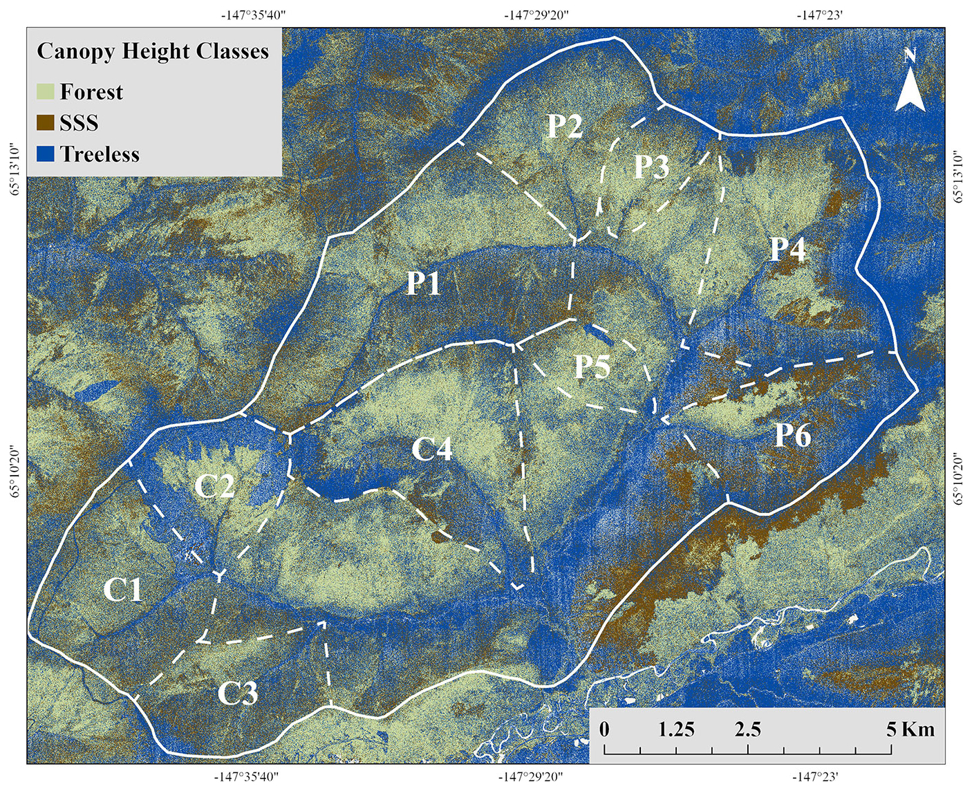
Figure 2 Canopy height map with color scale applied to show canopy height class distribution and subbasins (dashed white lines) within CPCRW (solid white line).

Table 1 Canopy height percentages for each of the watershed subbasins located within the CPCRW.

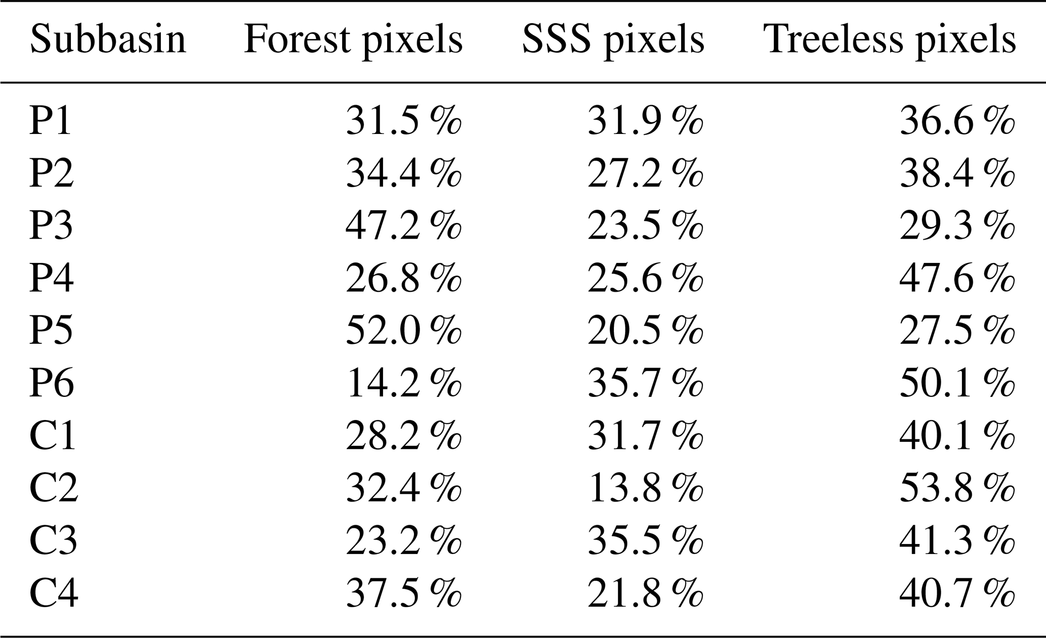
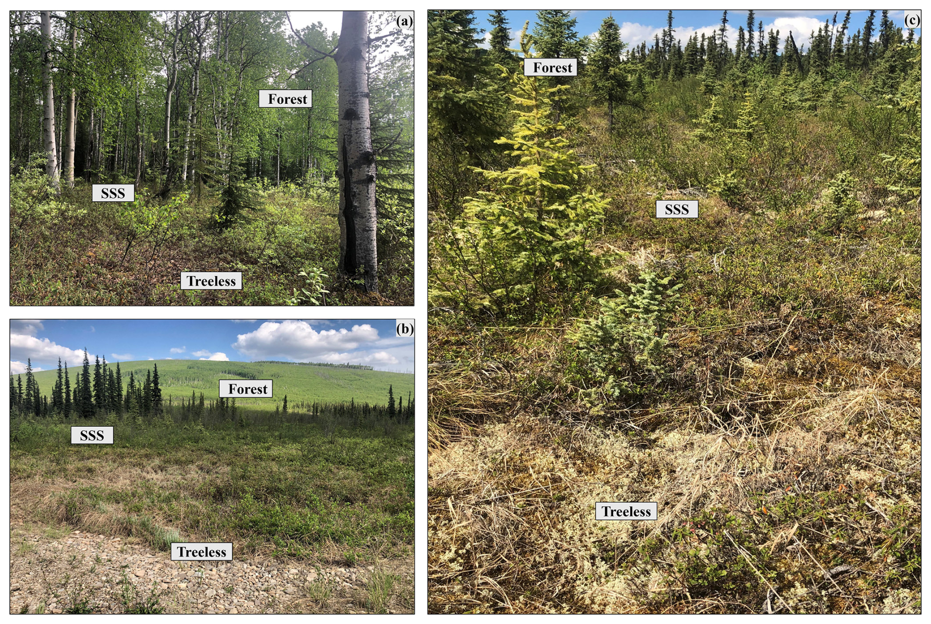
Figure 3 Photographs of the vegetative land cover taken in CPCRW on 2 June 2022, showing forest and understory examples of each canopy height class.

4.2 Comparison of ground-based and lidar-derived snow depths

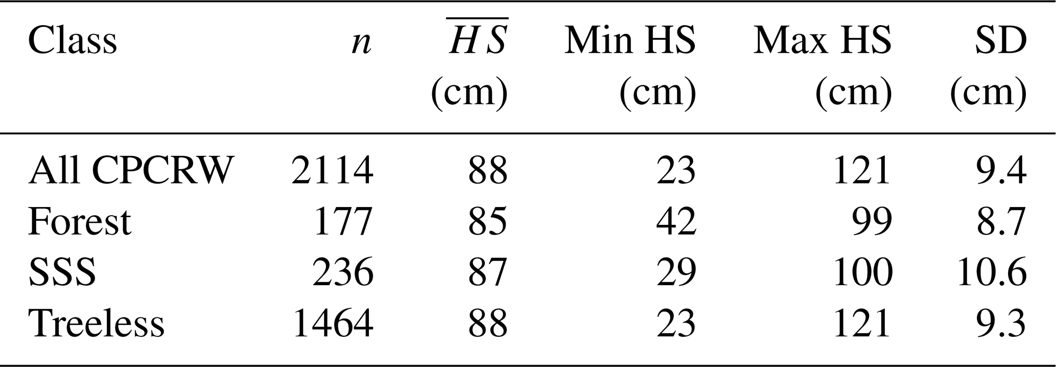
Ground-based snow depth measurements cover approximately 0.4 km² of the watershed area. The mean for all ground-based snow depths in the study site ($\stackrel{\mathrm{‾}}{HS}=\mathrm{88}$ cm) was similar to the mean snow depth calculated for ground-based measurements classified by canopy height forest ($\stackrel{\mathrm{‾}}{HS}=\mathrm{85}$ cm), SSS ($\stackrel{\mathrm{‾}}{HS}=\mathrm{87}$ cm), and treeless ($\stackrel{\mathrm{‾}}{HS}=\mathrm{88}$ cm) (Table 2). The range for all ground-based snow depths was 23–121 cm (Table 2).

Table 2 The mean manual snow depth ($\stackrel{\mathrm{‾}}{HS}$), range, standard deviation (SD), and number of ground-based measurements (n) recorded for the CPCRW and each canopy height class.

During March 2022 the snow depth at the USDA Caribou Snow Pillow snow course was 94 cm. This represents a 61 % increase from the 30-year median snow depth of 58 cm. At the USDA Caribou Creek snow course, the March 2022 snow depth was 89 cm, a 59 % increase from its 30-year median of 56 cm (USDA Natural Resources Conservation Service, 2022). These statistics demonstrate 2022 as an above-normal snowpack year.

The lidar data review resulted in a plausible snow depth range of 0–180 cm, which represents 99.98 % of the snow-covered area sampled by lidar. The remaining 0.02 % represents pixels that were located surrounding gaps (no data pixels) in the lidar, adjacent to structures, along trails, or scattered in patterns that do not reflect natural snowpack conditions. These pixels were omitted from the analysis.

Ground-based and lidar-derived snow depths were compared to quantify lidar accuracy and analyze snow depth variability within the study site. The average lidar-derived snow depth and standard deviation at in situ (ground-based) locations, at the study site, and in each canopy height class can be found in Table 3. For the study site, the mean lidar snow depth was calculated to be 98 cm (Table 3). The mean lidar snow depth at in situ locations was 90 cm. As suggested by this research, the sample variance of snow depths from airborne lidar minimally exceeds the sample variance from ground-based snow depths at the study site. The mean lidar-derived snow depths at collocated in situ locations was 2 cm more than the magnaprobe measurements from March 2022, and the mean lidar snow depth for the entire study site was 10 cm more than the magnaprobe measurements. Calculated standard deviations indicate that ground-based snow depth measurements vary by 9 cm, whereas lidar-derived snow depths for the study site vary by 15 cm. At the subbasin level, the mean lidar snow depths for all subbasins varied by 11 cm, with standard deviations ranging from 12–17 cm (Fig. 4). When comparing mean snow depths with the two snow course snow depths (89 and 94 cm), ground-based mean snow depths were all lower, while mean lidar snow depths were all between, or above, the snow course snow depths. The mean lidar snow depths for canopy height classes increased by 5 cm for forest, 15 cm for SSS, and 14 cm for treeless when compared to the corresponding mean snow depth at in situ locations based on canopy height. A box and whisker plot representing the mean lidar snow depth and standard deviation for the subbasins is found in Fig. 4.

Table 3 The mean lidar-derived snow depth ($\stackrel{\mathrm{‾}}{HS}$), standard deviation (SD), and number of lidar pixels (n) for the study site and canopy height classes.

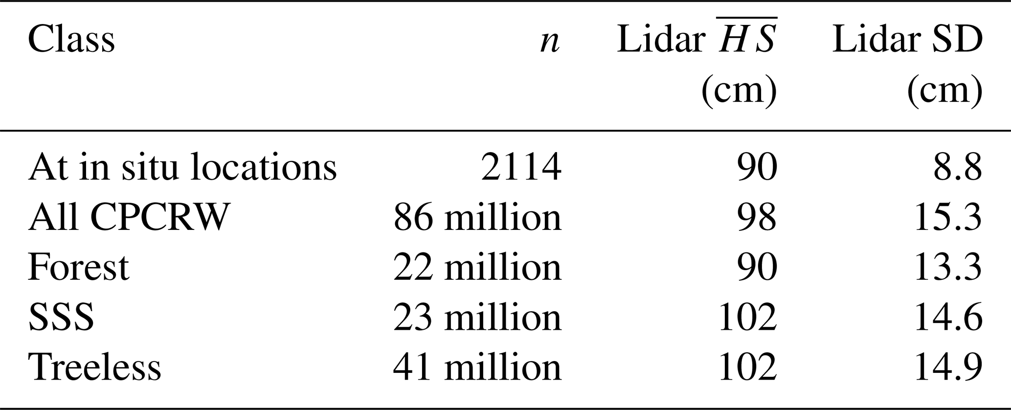
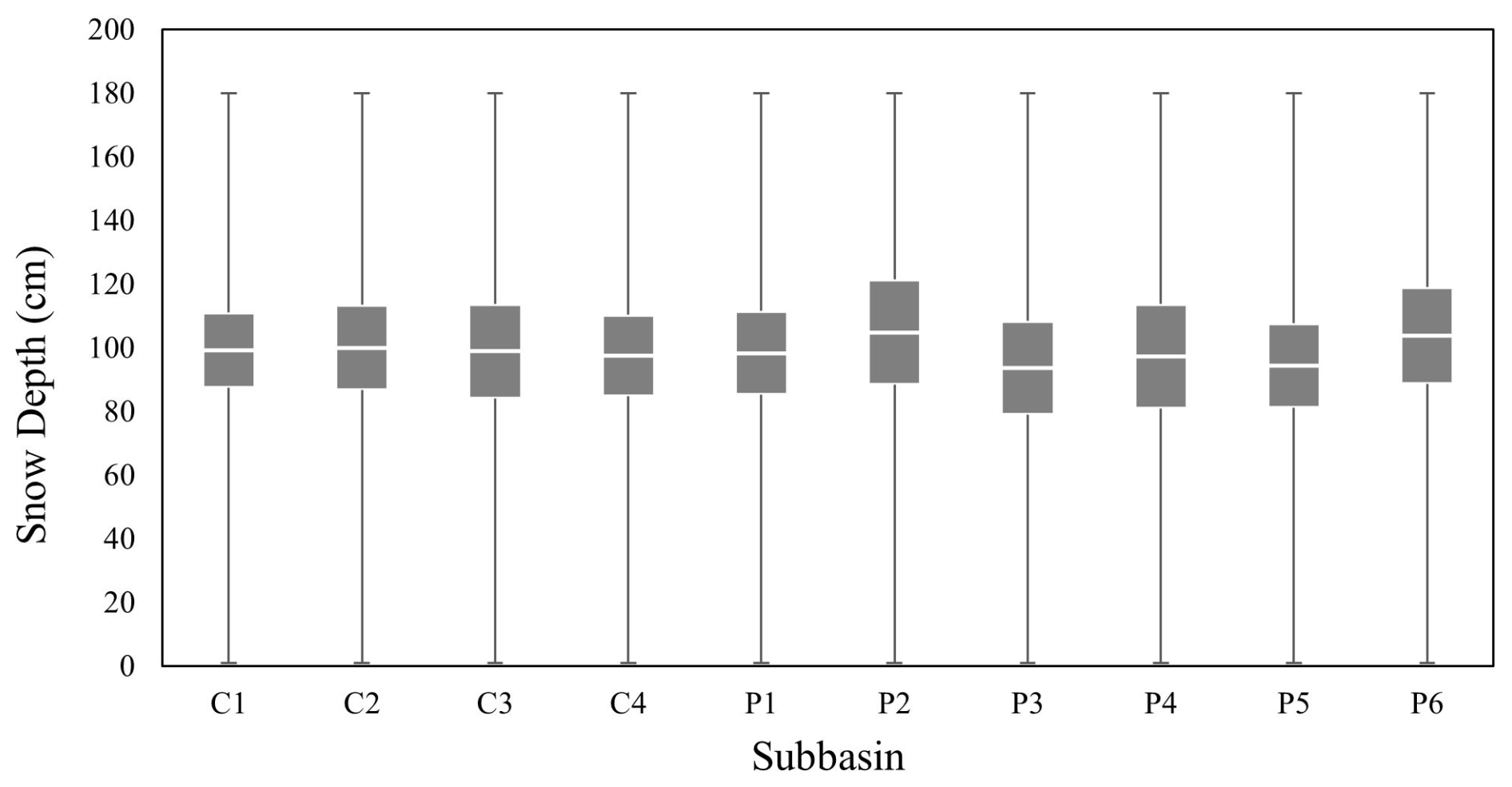
Figure 4 Box and whisker plot representing lidar snow depths within each subbasin in the CPCRW. The white bar represents the mean lidar snow depth, the gray boxes represent ±1 standard deviation, and the whiskers represent the minimum and maximum lidar snow depth within each subbasin.

To quantify lidar accuracy, lidar-derived snow depths and concurrent ground-based snow depths were compared statistically. A scatterplot for all ground-based and lidar-derived snow depths, and a corresponding 1:1 line, is displayed in Fig. 5. Error statistics from the lidar validation analysis produced a bias of 2.0 cm, an RMSE of 12.0 cm, and an R² value of 0.012 (Fig. 5). Error statistics and scatterplots for ground-based and lidar-derived snow depths based on canopy height resulted in a bias of 2 cm and an RMSE of 12 cm for SSS and treeless and a bias of 0 cm and an RMSE of 12 cm for forest (Fig. 5). All three canopy height classes had low R² values (Fig. 5).

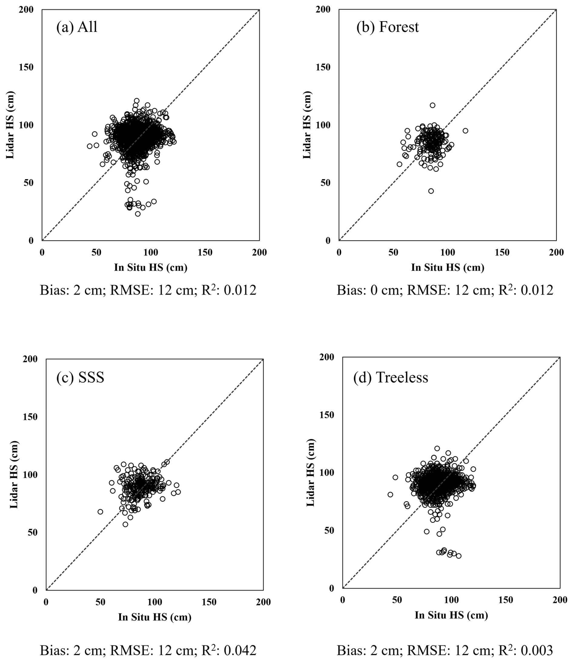
Figure 5 Scatterplots comparing ground-based snow depths with collocated lidar snow depths with a corresponding 1:1 line for all ground-based measurements within CPCRW (a), as well as for ground-based measurements classified into forest (b), SSS (c), and treeless (d) canopy height classes. Error statistics for each classification are displayed.

4.3 Statistical analysis of lidar-derived snow depths based on canopy height

To statistically compare lidar-derived snow depths between canopy height classes, it was necessary to create a snow depth map with independent observations that had eliminated spatial autocorrelation. The semivariogram analysis showed the average semivariogram range for the lidar-derived snow depth map to be 1.0 m. The lidar snow depth map was resampled to a 1.5 m spatial resolution to eliminate spatial autocorrelation. The lidar canopy height map was resampled to a 1.5 m spatial resolution to correspond to the lidar snow depth map pixel size.

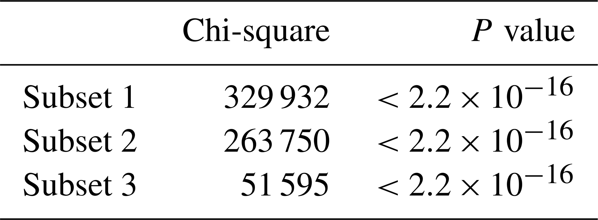
The lidar-derived snow depths and canopy heights from the three spatial subsets were used as variables to run the statistical Kruskal–Wallis test. Results of the Kruskal–Wallis test (Table 4) show that the p values comparing lidar-derived snow depths with canopy height are below the required value for significance (p value<0.05). A small p value and a large chi-square statistic allowed for a rejection of the null hypothesis, which states that the median lidar-derived snow depths between the canopy height classes are equal. A rejection of the null hypothesis supports the finding that there is a statistically significant difference in snow depths between canopy height classes for all three spatial subsets.

Table 4 Results of the Kruskal–Wallis test comparing median lidar snow depths based on canopy height class for each subset.

After a statistically significant difference in lidar-derived snow depths for the three spatial subsets was determined, the Wilcoxon rank sum test was used to calculate the p value of the median snow depth between specific canopy height pairs. The results of the Wilcoxon rank sum test show a statistically significant difference in the snow depth medians between each of the following canopy height pairs: SSS and forest, treeless and forest, and treeless and SSS had a p value of $<\mathrm{2}\times {\mathrm{10}}^{-\mathrm{16}}$ for all three subsets, except treeless and SSS for subset 2, which had a p value of $<\mathrm{6.2}\times {\mathrm{10}}^{-\mathrm{5}}$.

4.4 Influence of canopy height on snow depth estimation

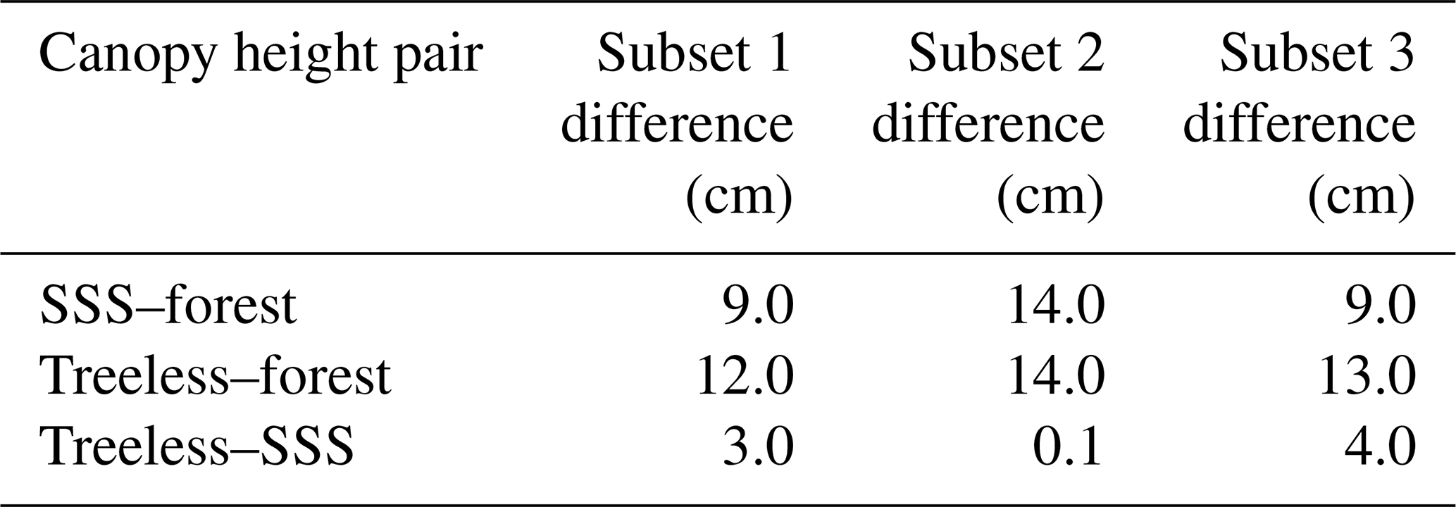
To analyze the influence of canopy height on snow depth distribution within the study site, the snow depth difference between specific canopy height pairs was calculated. This result was accomplished by observing the pairwise difference in median snow depths calculated by the Wilcoxon rank sum test. The pairwise difference was used to estimate the lidar snow depth variability between each canopy height pair. The difference in mean lidar-derived snow depths between each canopy height pair for the three spatial subsets is shown in Table 5. Two canopy height class pairs, SSS and forest as well as treeless and forest, had mean snow depth differences that were greater than the ±5 cm lidar vertical accuracy range for all three spatial subsets. When comparing the mean snow depth differences between these two class pairs, SSS averaged 9–14 cm more snow than forest (Table 5), and treeless averaged 12–14 cm more snow than forest (Table 5) for all three spatial subsets. This difference in snow depths is equivalent to an SWE range of approximately 20–30 mm. Canopy height SSS averaged slightly less snow than treeless, but the mean snow depth differences for the three spatial subsets fell within the ±5 cm lidar vertical accuracy range.

Table 5 Difference in mean lidar-derived snow depth between canopy height class pairs. The mean snow depth of the second class listed is subtracted from the mean snow depth of the first class listed.

5 Discussion

5.1 Sources of error and uncertainty in lidar-derived snow depths

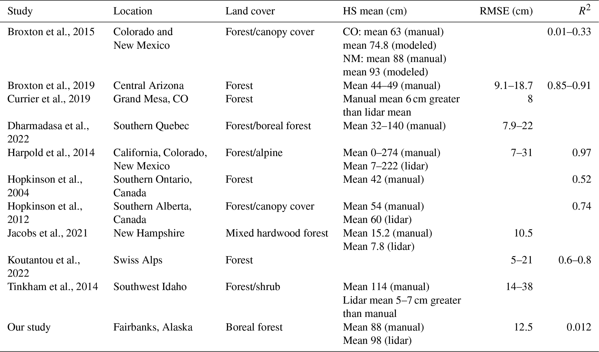
Ground-based snow depth measurements provide an independent data set for the assessment of errors and uncertainties in data collected remotely. A total of 10 previous studies that used ground-based measurements to validate airborne lidar (Table 6) in forested areas found RMSEs ranging from 3 to 37 cm. Koutantou et al. (2022) found that their boreal forest site had the highest RMSE (19–22 cm) compared to their deciduous forest and field sites. This study's calculated RMSE for comparing lidar-derived snow depths with ground-based measurements (RMSE=12.5 cm) falls within a range that is generally acceptable for most research (Harpold et al., 2014). However, the coefficient of determination between ground-based and lidar-derived snow depths (R²=0.012) is considerably lower for this study compared to the studies listed in Table 6. We suggest that the low correlation between our lidar-derived and ground-based snow depth measurements is primarily due to vegetation, specifically the dense understory. A prominent non-processing source of error in airborne lidar data is vegetation-induced errors (Deems et al., 2013). Deems et al. (2013) found that the ground return point density decreases inversely with canopy and subcanopy density and is influenced by canopy and understory structure. Reutebuch et al. (2003) found that when using airborne lidar to measure ground elevations in a forested area, the accuracy of the ground points was reduced by approximately 10 cm because the dense canopy and understory vegetation reduced the strength of the return signal back to the sensor, making it harder to precisely pinpoint the ground surface. Prior studies noted similar lidar errors occurring in vegetative landscapes where shrubs were prominent (Contreras et al., 2017; Gould et al., 2013; Spaete et al., 2011). The dense understory of the canopy height classes of SSS and treeless areas, which comprise approximately 74 % of CPCRW (Fig. 3), prevents lidar laser pulses from reaching and accurately mapping the ground surface. During snow-on acquisition dense ground vegetation could further introduce error into the snow-on DTM by compacting beneath the snowpack or elevating snow on top of dense vegetation. Errors in both snow-free and snow-on DTMs caused by the dense understory can lead to a less accurate snow depth map, which in turn affects the correlation between ground-based and lidar-derived snow depth measurements.

Table 6 Studies that compare lidar-derived snow depths with manual snow depth measurements are listed in the table. Information on location, land cover type, manual and lidar snow depth means, and error statistics are provided for each study.

In addition to the dense understory, further explanations for a low R² value could include sampling restrictions and spatial scale. Ground-based snow depth measurements were clustered together and occurred at lower elevations as a result of difficult terrain and limited access within the study site. The magnaprobe GPS units have a horizontal positioning error of ±2.5 m in open areas and 10–15 m in dense forest, which could impact the correlation of ground-based snow depths with collocated lidar-derived snow depths. Efforts to minimize positioning errors involved taking ground-based measurements approximately 1–3 m apart, followed by visually inspecting the measurement pattern for outliers and ensuring alignment with a road or a trail. Lastly, snow depth variability at the sub-meter scale could be influencing the low R² values when we compare a single magnaprobe measurement to its collocated lidar pixel. During the March 2022 SnowEx field campaign, evidence of snow depth variability over a single meter of distance was repeatedly seen in all vegetation types while taking ground-based measurements. Tussocks, understory brush, downfall, and the snowpack itself all impacted snow depths within a meter. Ground-based snow depth variability observed on a sub-meter scale, in all three canopy height classes, supports the calculated semivariogram range of 1.0 m for spatial autocorrelation.

While sub-meter snow depth variability can be high (Komarov and Sturm, 2023), we found that when comparing snow depth variability at the watershed scale, all ground-based, lidar, and canopy height mean snow depths fell within 1 standard deviation of each other, which represents 10 %–16 % of the mean snow depth (Table 3). Results from an analysis performed using ground-based and airborne lidar data from the March 2023 SnowEx Alaska campaign for this study site found similar statistical results (16 %–18 % of mean snow depth). This provides evidence of consistently lower variability in snow depths at the mesoscale over two snowpack years at CPCRW.

5.2 Implications for water and resource management

Water and resource managers use snow data, including snow depth and SWE, to assess the availability of water resources in regions dependent on snowmelt (Dickerson-Lange et al., 2021; Siirila-Woodburn et al., 2021). Our study site had a mean lidar snow depth of 98 cm, which is equivalent to approximately 210 mm of SWE. When comparing median snow depths our analysis showed a statistically significant difference in median snow depths between all canopy height classes, with differences in snow depths, based on canopy height, equivalent to an SWE range of roughly 20–30 mm. This information can be utilized by water and resource managers to make informed decisions about water supply, flood control, evaluating the impact of climate change on precipitation and snow accumulation/melt patterns, land use decisions, and wildlife and conservation efforts (Dickerson-Lange et al., 2021; Hopkinson et al., 2004; Mazzotti et al., 2019; Reinking et al., 2022; Webb et al., 2020).

Snow data obtained through various platforms, including ground-based, aircraft, satellite, or estimated through modeling tools, can be incorporated together to produce more accurate and sophisticated spatiotemporal snow distribution estimations than are possible with any single measurement technique performed alone (Boelman et al., 2019; Stuefer et al., 2013). Our study used ground-based measurements to validate an airborne lidar snow depth map in a boreal forest ecotype. As evidenced in Table 6, only one additional study that compared ground-based measurements to airborne lidar occurred within a boreal forest site. The comparison of ground-based measurements to airborne lidar by Dharmadasa et al. (2022) produced an RMSE of 19–22 cm at their boreal forest site. Our study produced an RMSE of 12.5 cm when validating airborne lidar with ground-based snow depth measurements. Validated lidar snow depth maps have advanced our ability to characterize the spatial variability in snow depths at a watershed scale and, when coupled with an airborne lidar canopy height map, can be applied to snow and hydrological modeling applications to improve hydrological forecasts and SWE estimates at even larger regional or global scales (Deems et al., 2013; Hopkinson et al., 2004, 2012; Jacobs et al., 2021; Nolan et al., 2015; Painter et al., 2016; Trujillo et al., 2007). To further improve validated lidar snow depth maps, future snow research occurring in boreal forests should include snowpack profile measurements that could be used to identify and quantify vegetation-induced errors in ground-based measurement techniques and airborne lidar data products associated with the complicated and dense boreal forest understory.

Accurately accounting for vegetation effects on snow storage and distribution is important as forests are changing due to warming climate conditions, forest disturbances, wildfires, insect infestation, and permafrost degradation (Panda et al., 2010; Smith et al., 2021). These changes are occurring in boreal forests, but research is limited as to how Alaska boreal forest vegetation impacts snow distribution. A literature review found one study occurring in an Alaska boreal forest, by Douglas and Zhang (2021), that looked at vegetation impacts on snow storage using lidar and machine learning. They found that in their Alaska boreal forest sites mixed forest ecotypes had the shallowest snowpack, while tussock tundra (equivalent to our treeless) and moss spruce forest (equivalent to our SSS) were associated with the deepest snowpack. The results of our vegetation analysis show that canopy height has a statistically significant effect on the spatial variability of snow depths at our study site. The canopy height pairs of SSS and forest as well as treeless and forest had snow depth differences that fell outside the lidar error range for all three spatial subsets and differed in SWE by 10 mm. The canopy height pair of treeless and SSS yielded results that fell within the lidar error range for all three spatial subsets, making it difficult to clearly attribute snow depth variability between the two classes to vegetation or lidar accuracy. This result implies that there is less variability in snow depths between treeless and SSS canopy height classifications. In terms of canopy height classification, two canopy height classes of less than 5 m and greater than 5 m could be sufficient to quantify the mean snow depths in CPCRW.

6 Conclusion

Despite considerable literature on airborne lidar snow depth retrievals in forested environments, little research has been published on its ability to measure snow depth in boreal forests. We demonstrate the utility of a high-resolution airborne lidar snow depth map to characterize the spatial variability of snow depths within a boreal forest study site where snow remote sensing research is limited. The validation efforts showed that lidar-derived snow depths had an RMSE of 12.0 cm and a bias of 2.0 cm when compared to data from 2114 ground-based field measurements. While these results show a statistically significant relationship between lidar-derived snow depths and manual field measurements, errors and uncertainties caused by dense understory vegetation need to be considered with detailed snowpack profile measurements. We further demonstrate that an airborne lidar canopy height map can be used to analyze the impact of vegetation on snow depth variability in a complex boreal forest ecosystem and that two canopy height classes may be sufficient to characterize the snow depth spatial variability therein.

Lastly, we show that snow depth variability between subbasins within CPCRW, and at the watershed scale, is 10 %–16 % of the mean snow depth. This is evidenced by all mean snow depths (ground-based, lidar, canopy height class, subbasins, and overall) occurring within 1 standard deviation of each other. This study demonstrates that airborne lidar-derived data products can effectively estimate and quantify the variability of snow depths in an Alaska boreal forest but should be validated and assessed for vegetative errors using ground-based measurements.