Changes in Antarctic surface conditions and potential for ice shelf hydrofracturing from 1850 to 2200

A mixed statistical–physical approach is used to emulate the spatio-temporal variability of the Antarctic Ice Sheet surface mass balance and surface melt rates of a regional climate model. We demonstrate the ability of this simple method to extend existing regional climate simulations to periods, scenarios, or climate models that were not originally simulated. This method is useful to quickly populate ensembles of surface mass balance and melt rates, which are needed to constrain ice sheet model ensembles. Here we apply this method to estimate (i) the changes in Antarctic surface mass balance over 1850–2200 and the associated effect on sea level and (ii) the changes in potential for ice shelf hydrofracturing.

After weighting 16 climate models to obtain a realistic distribution of the equilibrium climate sensitivity, we find a likely contribution of surface mass balance to sea level rise of −2.2 to −0.4 cm from 1900 to 2010 and −3.4 to −0.1 cm from 2000 to 2099 under the SSP1-2.6 scenario versus −4.4 to −1.4 cm under SSP2-4.5, and −7.8 to −4.0 cm under SSP5-8.5. The contribution from 2000 to 2200 is highly uncertain: between −10 and −1 cm in SSP1-2.6 and between −33 and +6 cm in SSP5-8.5 depending on the climate model.

Based on a criterion on the presence of liquid water beyond firn saturation in our emulated ensemble, we estimate the surface conditions that make ice shelves prone to hydrofracturing. Our results suggest that a majority of Antarctic ice shelves could remain safe from hydrofracturing under the SSP1-2.6 scenario, but all of them could become prone to hydrofracturing before 2150 under the SSP5-8.5 scenario.

1 Introduction

In the 21st century, increasing snowfall over the Antarctic Ice Sheet is expected to compensate a significant part of the dynamical ice mass loss triggered by ocean warming, which mitigates the Antarctic contribution to sea level rise (e.g. Seroussi et al., 2020; Edwards et al., 2021; Fox-Kemper et al., 2021). However, models suggest that if air temperatures exceed ∼ 7.5 °C above the 1981–2010 average, the increase in accumulation starts to be overwhelmed by the mass loss through surface meltwater runoff into the ocean (Kittel et al., 2021; Coulon et al., 2024).

Runoff is a negative contribution to the surface mass balance. It is produced if surface melt and/or rain rates are high enough to (i) percolate and bring the temperature of underlying snow and firn layers to the freezing point; (ii) saturate the pore space in the snow and firn layers, which is sometimes referred to as firn air depletion (Pfeffer et al., 1991; Kuipers Munneke et al., 2014; Alley et al., 2018); and (iii) flow into the ocean. The liquid water beyond firn saturation, hereafter often referred to as excess liquid water, does not necessarily flow into the ocean, especially in the case of a relatively flat surface. Excess liquid water can indeed alternatively form ponds or be transported horizontally within the firn or at the ice surface (Kingslake et al., 2017; Bell et al., 2018).

The presence of excess liquid water can trigger ice shelf break-up through hydrofracturing: in favourable conditions of ice shelf stress, the weight of liquid water can destabilize a fracture and lead to its unstoppable propagation as long as liquid water keeps filling the fracture (Weertman, 1973; Lai et al., 2020). Stress variations associated with surface meltwater ponding and drainage, causing flexure and fracture, can amplify this mechanism and propagate its effects spatially (Banwell et al., 2013, 2019). An entire ice shelf break-up nonetheless likely requires high meltwater production all over its surface, as observed before the break-up of Larsen A in 1995 and Larsen B in 2002 (Skvarca et al., 2004; Scambos et al., 2003; van den Broeke, 2005; Sergienko and Macayeal, 2005; Robel and Banwell, 2019; Wille et al., 2022).

When occurring on ice shelf parts that buttress the upstream flow, hydrofracturing and the resulting ice shelf collapse may strongly enhance the contribution of upstream glaciers to sea level rise (Fürst et al., 2016; Sun et al., 2020; Seroussi et al., 2024). Gilbert and Kittel (2021) estimated that 34 % of Antarctic ice shelf area could be vulnerable to hydrofracturing at 4 °C of warming above pre-industrial levels. The exact warming level needed to trigger the widespread presence of liquid water on a given ice shelf depends on the amount of snowfall and the snow/firn temperature and density (Donat-Magnin et al., 2021; van Wessem et al., 2023).

The contribution of ice sheets to changes in sea level are estimated through ice sheet simulations driven, among other things, by spatio-temporal variations in surface mass balance (SMB) and sometimes by the dates of collapse for individual ice shelves. In the Ice Sheet Model Intercomparison Project for the sixth Coupled Model Intercomparison Project (CMIP6, Eyring et al., 2016; ISMIP6, Nowicki et al., 2016), these conditions were directly calculated from CMIP model outputs (Nowicki et al., 2020; Seroussi et al., 2024). Despite progress in their representation of the Antarctic climate (Dunmire et al., 2022), the CMIP models often have a coarse resolution and include a relatively poor representation of snow processes over ice sheets, in particular with regard to firn saturation by meltwater and subsequent ponding or runoff (Nowicki et al., 2020).

Regional climate models (RCMs) dedicated to polar regions and constrained by CMIP projections offer a good alternative to the direct use of CMIP models for the estimation of surface conditions (e.g. Kuipers Munneke et al., 2014; Kittel et al., 2021). Despite detailed snow physics, a major weakness of RCMs is nonetheless the associated requirement for additional skills and processing/computing time, which is why RCM outputs were not ready on time for ISMIP6-Antarctica (Nowicki et al., 2020; Seroussi et al., 2020). Because of these difficulties, only a limited number of RCM-based projections is usually produced, which is generally insufficient to sample the CMIP model diversity. This may affect the representation of the recent period (Barthel et al., 2020) and the sensitivity to increasing anthropogenic emissions (e.g. Hausfather et al., 2022) in the small RCM ensemble.

Over the years, Antarctic Ice Sheet modellers have often scaled their best estimates of present-day accumulation to temperature anomalies from the CMIP models (e.g. based on the Clausius–Clapeyron relationship as in Gregory and Huybrechts, 2006), while positive degree-day models have sometimes been used to derive melt rates (e.g. Rodehacke et al., 2020; Zheng et al., 2023). The latter are based on daily air temperatures projected by the CMIP models and can be calibrated to match RCM projections (Coulon et al., 2024). Other methods are emerging based on the emulation of more complex models like RCMs (van der Meer et al., 2023) or firn models (Dunmire et al., 2024). In this paper, we present and evaluate a novel statistical–physical method that emulates the spatio-temporal evolution of the surface mass balance (SMB) and surface melt rates of a regional climate model (Sect. 2). This method is applied in Sect. 3 to provide confidence intervals on the changes in SMB and the associated changes in sea level and on the changes in production of excess liquid water and the implications for ice shelf hydrofracturing.

2 Methods

2.1 Approach

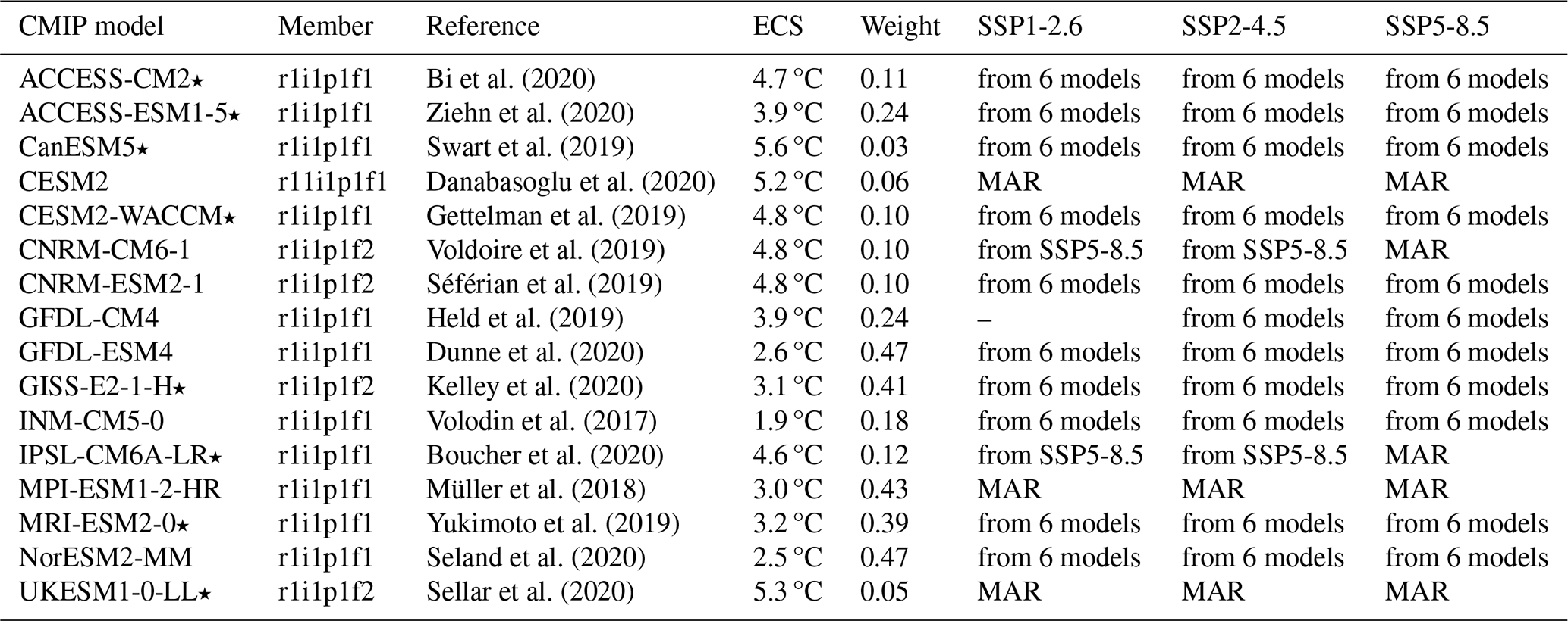
Here we estimate both the SMB evolution over the grounded ice sheet for its equivalent change in global sea level and the evolution of the liquid water production beyond firn saturation for its potential to induce hydrofracturing. We build an ensemble of estimates over Antarctica, for the 1850–2100 period, driven by 16 CMIP6 models and 3 SSP (Shared Socioeconomic Pathway; O’Neill et al., 2014) scenarios (Table 1). A smaller ensemble covers the 1850–2200 period, driven by only eight CMIP6 models (see stars in Table 1) and two SSP scenarios (SSP1-2.6 and SSP5-8.5).

Our approach is based on a limited number of RCM simulations covering 1980–2100 or 1980–2200 (Sect. 2.2), and the full ensemble is populated using a statistical–physical emulation method (Sect. 2.3). The emulation method can be used to extend a given RCM simulation in time, to produce data for a scenario that was not covered by the RCM, or to produce data for a CMIP model that was never used to force the RCM (Fig. 1). These approaches are first evaluated separately (Sect. 2.3.3 to 2.3.5), and then they are combined (Sect. 2.4) to produce the ensemble projections described in Sect. 3.

Bi et al. (2020)Ziehn et al. (2020)Swart et al. (2019)Danabasoglu et al. (2020)Gettelman et al. (2019)Voldoire et al. (2019)Séférian et al. (2019)Held et al. (2019)Dunne et al. (2020)Kelley et al. (2020)Volodin et al. (2017)Boucher et al. (2020)Müller et al. (2018)Yukimoto et al. (2019)Seland et al. (2020)Sellar et al. (2020)

Table 1 CMIP6 models used to drive MAR simulations or emulations until 2100 in Sect. 3. ECS stands for equilibrium climate sensitivity, and the indicated values are from Meehl et al. (2020), except for NorESM2-MM, which is from Seland et al. (2020). Stars beside model names indicate that the CMIP6 simulations were extended to 2200 under the SSP1-2.6 and SSP5-8.5 pathways. The entries for the three SSP pathways indicate whether it was derived from the actual MAR simulation driven by this CMIP model under this scenario (MAR), from a MAR simulation driven by this CMIP model but for a warmer scenario (“from SSP5-8.5”, i.e. method described in Sect. 2.3.4), or emulated from six MAR simulations driven by different CMIP models (“from 6 models”, i.e. method described in Sect. 2.3.5). The historical period was directly available from the five CMIP models for which at least one MAR projection was available, and it was emulated from six models for the other CMIP models.

2.2 Regional climate model projections

We make use of the MAR-3.11 regional climate model (Gallée and Schayes, 1994; Gallée, 1995; Kittel et al., 2021, 2022), which parameterizes multiple processes relevant for polar environments. In MAR, the atmosphere is coupled to a 30-layer model representing the first 20 m of snow/firn with a refined resolution at the surface. The snow/firn model solves prognostic equations for temperature, mass, water content, and snow properties (dendricity, sphericity, and grain size). In the presence of surface melting or rainfall, liquid water percolates downward into the next firn layers with a water retention of 5 % of the porosity in each successive layer. The firn layers are fully permeable until they reach a close-off density of 830 kg m⁻³. To account for possible cracks in ice lenses and moulins, the part of available water that is transmitted downward to the next layer decreases as a linear function of firn density, from 100 % transmitted at the close-off density to zero at 900 kg m⁻³ and beyond. If liquid water is not able to percolate further down, it remains where it is. When the entire porosity space in the uppermost snow/firn layer is filled with liquid water or if the uppermost snow/firn layer is denser than 900 kg m⁻³, any additional surface melt is considered runoff and removed from the snow/firn model. There is no representation of ponds or horizontal routing.

The surface mass balance and melting conditions produced by MAR have been evaluated in comparison to observational products in several studies, and a qualitative comparison to a satellite estimate of melt pond volume indicates that MAR is able to capture the main characteristics of the present-day surface conditions (Appendix A).

The MAR simulations were run at 35 km resolution, and the outputs were conservatively interpolated onto a 4 km stereographic grid following the atmospheric forcing protocol in ISMIP6. Unless specified otherwise, we use these 4 km data, and all spatial integrals presented in this study were calculated by accounting for the stereographic scale factor. The ice mask and the surface elevation are based on Bedmap2 (Fretwell et al., 2013). The actual grounded ice sheet and ice shelf areas are 12.286 and 1.737 million km², respectively.

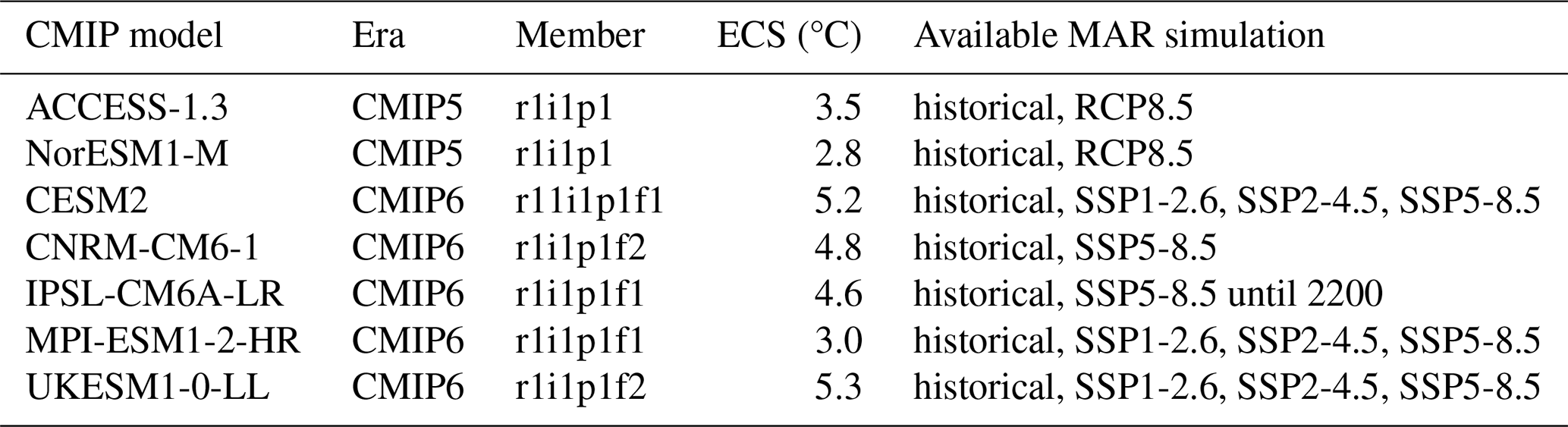
Our MAR simulations cover 1980–2100 and are driven by two CMIP5 and five CMIP6 models under a number of scenarios, as listed in Table 2. The MAR–IPSL-CM6A-LR projection goes until 2200 following the extended SSP5-8.5 scenario (Shared Socioeconomic Pathway; Meinshausen et al., 2020). The selection of these specific CMIP models was based on the availability of 6-hourly outputs (required to provide MAR boundary conditions), the evaluation of their present-day mean characteristics (Agosta et al., 2019, 2024; Barthel et al., 2020), and the diversity of their sensitivity to anthropogenic emissions. The final criterion is characterized by the equilibrium climate sensitivity (ECS (Hausfather et al., 2022)), which is the increase in global mean surface air temperature that follows a doubling of atmospheric carbon dioxide.

For computational reasons, all simulation years were run in parallel with 20 years of spin-up to equilibrate the firn properties (e.g. 2051 is spun up from the transient 2031–2050 period). The initial state (e.g. 1 January 2031 for the simulation of 2051) is taken from the MAR–ACCESS-1.3 RCP8.5 simulation (Table 2), itself spun up from a previous version of MAR at 50 km resolution driven by NorESM1-M under RCP8.5 and spun up for 30 years from a present-day MAR simulation. A spin up of 20 years is generally sufficient to remove any sensitivity to the initial state (Donat-Magnin et al., 2021, their Fig. 12).

Table 2 List of CMIP models, their ensemble member number, their equilibrium climate sensitivity (ECS; provided by Meehl et al., 2020) and the scenarios for which we have a MAR simulation driven by this CMIP model. The historical MAR simulations only start in 1980, and the projections go until 2100 unless specified otherwise. The model references are provided in Table 1.

2.3 Statistical–physical emulation method

Hereafter, we first describe how the RCM projections of surface mass balance, surface melting, and production of liquid water beyond firn saturation can be extended in time and to other scenarios or CMIP models. Then, we evaluate these emulated projections in comparison to the actual RCM projections. In this subsection, we assume that runoff is equal to the production of liquid water beyond firn saturation as in the RCM, but we use a different approach for the projections presented in Sect. 3.

2.3.1 Rationale

Precipitation in Antarctica mostly consists of snowfall even in a warmer climate (Kittel et al., 2021; Donat-Magnin et al., 2021; see also Appendix B). In the first approximation, snowfall in Antarctica (SNF) thus increases with air temperature following the Clausius–Clapeyron law, which can be approximated as follows:

$$\begin{array}{}\text{(1)}& \mathrm{SNF}\left(T_{\mathrm{ref}}+\mathrm{\Delta }T\right)=\mathrm{SNF}\left(T_{\mathrm{ref}}\right)\times e^{a\mathrm{\Delta }T},\end{array}$$

where T_ref is a reference air temperature, ΔT the air warming, and a typically 0.07 in polar conditions (Donat-Magnin et al., 2021).

Previous modelling studies also found an empirical exponential relationship between the surface melt rate (MLT) and air warming:

$$\begin{array}{}\text{(2)}& \mathrm{MLT}\left(T_{\mathrm{ref}}+\mathrm{\Delta }T\right)=\mathrm{MLT}\left(T_{\mathrm{ref}}\right)\times e^{b\mathrm{\Delta }T},\end{array}$$

where b is typically between 0.3 and 0.6 in Antarctica (Trusel et al., 2015; Donat-Magnin et al., 2021). In the following, we assume that ΔT is a variation in near-surface air temperature in both Eqs. (1) and (2), which is a reasonable approximation given that the troposphere warms relatively uniformly from the surface to ∼ 300 hPa (Donat-Magnin et al., 2021, their Fig. 1).

Then, we introduce the r parameter, a threshold over which liquid water is produced beyond firn saturation, which occurs when the melt rate exceeds what can be stored and refrozen in the ongoing snow/firn accumulation (Pfeffer et al., 1991; Kuipers Munneke et al., 2014; Donat-Magnin et al., 2021; van Wessem et al., 2023), i.e. if

$$\begin{array}{}\text{(3)}& {\displaystyle \frac{\mathrm{MLT}}{\mathrm{SNF}}}\ge r,\end{array}$$

where r is typically between 0.60 and 0.85 depending on the snow properties (Donat-Magnin et al., 2021). Here we do not attempt to determine whether the excess of liquid water forms ponds or flows directly into the ocean (runoff), which is why the same r value is used on the grounded ice sheet and on ice shelves.

In Eq. (3), the effect of rainfall, sublimation, and drifting-snow erosion are assumed to be negligible. Sublimation remains below 10 % of snowfall even in a warmer climate (Kittel et al., 2021, their Tables S2–S3), and drifting-snow erosion is at least an order of magnitude smaller than sublimation (Gadde and van de Berg, 2024). As shown in Appendix B, rainfall represents less than 15 % of the total precipitation on the grounded ice sheet until 2200 and on the ice shelves until 2100. The impact of neglecting rainfall in our method is discussed in Appendix B.

In this paper, we use these relationships to extrapolate the SMB, melt rates, and production of liquid water beyond firn saturation to warmer or colder surface conditions. We assume that all the quantities at near-surface air temperature T_ref are perfectly known from the RCM, and we want to estimate them for a temperature change of ΔT that is provided by a CMIP model. To do so, we use the following sequence of equations, in which RU is the rate of mass loss through runoff (<0), while surface melt rate is defined as positive:

$$\begin{array}{}\text{(4)}& \left\{\begin{array}{lll}\mathrm{SNF}\left(T_{\mathrm{ref}}+\mathrm{\Delta }T\right)& =& \left(\mathrm{S}\mathrm{M}\mathrm{B}\left(T_{\mathrm{ref}}\right)-\mathrm{RU}\left(T_{\mathrm{ref}}\right)\right)\times e^{a\mathrm{\Delta }T},\\ \mathrm{MLT}\left(T_{\mathrm{ref}}+\mathrm{\Delta }T\right)& =& min\left\{\mathrm{MLT}\left(T_{\mathrm{ref}}\right)\times e^{b\mathrm{\Delta }T},m\right\},\\ \mathrm{RU}\left(T_{\mathrm{ref}}+\mathrm{\Delta }T\right)& =& -max\left\{\mathrm{0},\mathrm{MLT}\left(T_{\mathrm{ref}}+\mathrm{\Delta }T\right)\right.\\ & & \left.-r\mathrm{SNF}\left(T_{\mathrm{ref}}+\mathrm{\Delta }T\right)\right\},\\ \mathrm{S}\mathrm{M}\mathrm{B}\left(T_{\mathrm{ref}}+\mathrm{\Delta }T\right)& =& \mathrm{SNF}\left(T_{\mathrm{ref}}+\mathrm{\Delta }T\right)\\ & & +\mathrm{RU}\left(T_{\mathrm{ref}}+\mathrm{\Delta }T\right),\end{array}\right.\end{array}$$

where a, b, m, and r are the method parameters. The m parameter is introduced to avoid unrealistically high melt rates. For the emulation, we assume that the emulated runoff (RU) is equal to the production rate of liquid water beyond firn saturation as in the RCM.

In Sect. 3, we emulate surface conditions for periods (Fig. 1a), scenarios (Fig. 1b), or CMIP models (Fig. 1c) that are not covered by existing MAR simulations. Our aim is to populate a large ensemble of surface conditions that can be used to drive ensembles of ice sheet and sea level projections without the cost of running many RCM simulations and the associated need for 6-hourly outputs in the corresponding CMIP simulations. We first assess the performance of the emulation method for other periods, scenarios, and CMIP models in Sect. 2.3.3 to 2.3.5, and then we combine them in Sect. 3 based on this assessment.

In this work, we use annual means for all the variables, which is consistent with usual datasets available for ice sheet models (e.g. Nowicki et al., 2020). To emulate a surface variable at a given warming or cooling level, we always calculate the emulation from 20 different years (i.e. different values of T_ref and ΔT), and then we average the 20 emulated values (Fig. 1). This is done to better sample natural variability and to generate an emulated variability that is mostly related to CMIP model temperatures. It also makes the emulation more robust from a statistical point of view.

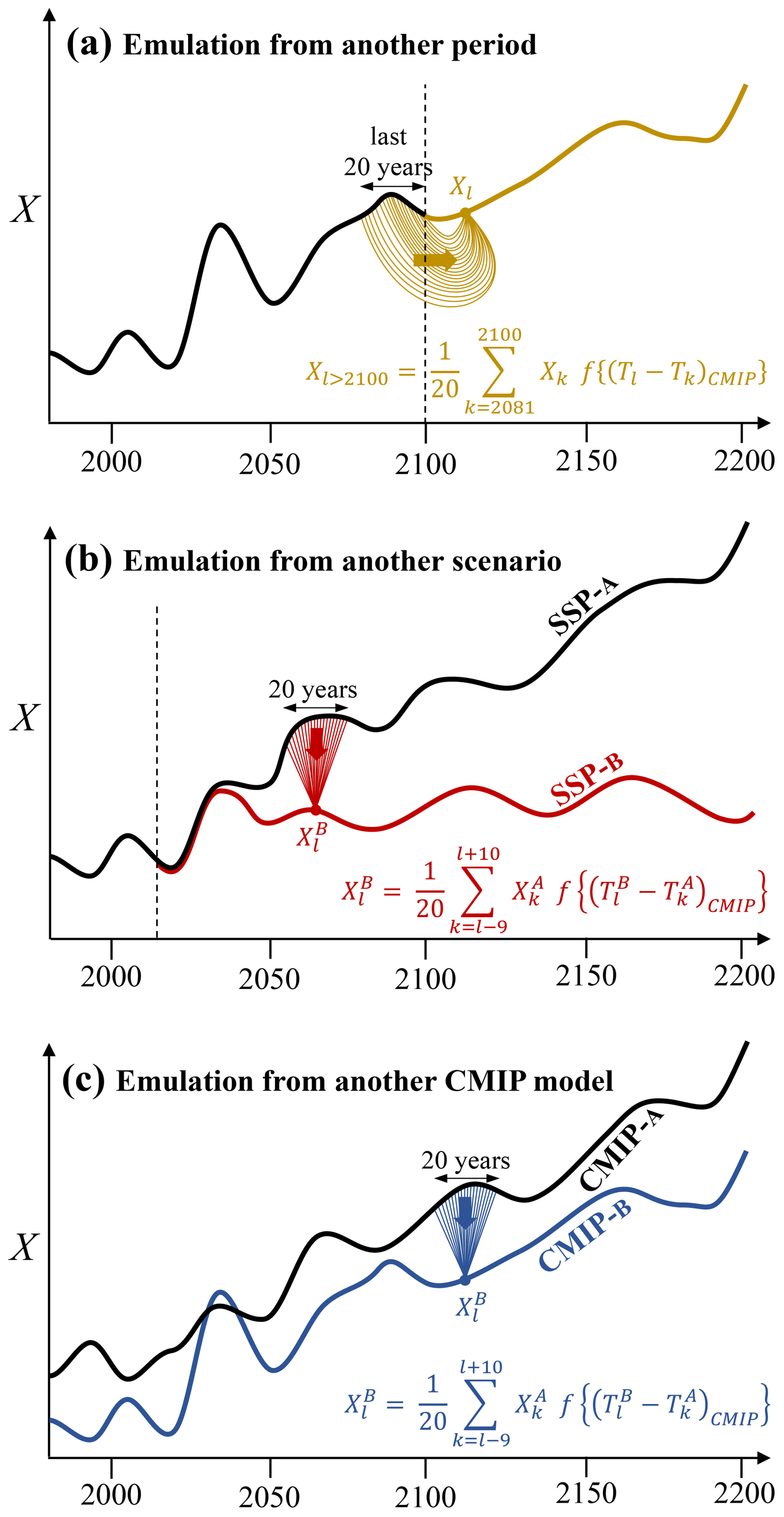
Figure 1 Schematic of the application of our emulation methodology (Eq. 4) to (a) extend the data to periods not simulated by MAR (Sect. 2.3.3), (b) extend the data to scenarios not simulated by MAR (Sect. 2.3.4), and (c) extend the data to CMIP models not downscaled by MAR (Sect. 2.3.5). Variable X represents either SMB or surface melt rate. Function f represents one of the functions of ΔT provided in Eq. (4).

2.3.2 Parameter calibration

The a and b parameters are obtained through a least-mean-squares fitting of an exponential curve for SMB minus model runoff on the one hand and for the surface melt rate on the other hand. Appendix C provides more details on the fitting method and gives the a and b values for individual models. On average, a=0.068, and b=0.320.

The maximum local melt rate (m parameter in Eq. 4) is set to the 99.99th percentile of 1980–2100 local melt rates ($m=\mathrm{1.80}\times {\mathrm{10}}^{-\mathrm{4}}$ $\mathrm{kg}{\mathrm{m}}^{-\mathrm{2}}{\mathrm{s}}^{-\mathrm{1}}$, i.e. 15.5 mm d⁻¹). The value of r is more difficult to calibrate as it depends on the density and temperature of snow and on the threshold used to consider the fact that liquid water is produced beyond firn saturation (Pfeffer et al., 1991; Donat-Magnin et al., 2021), so we assess values in the 0.50–0.90 range, which includes the values used in previous work.

2.3.3 Emulation from another period

We first assess the ability of our emulation method (Eq. 4) to extend a RCM simulation backward or forward in time, based on the air temperatures of the corresponding CMIP model over the extended periods (Fig. 1a). The benefits of this method would be to extend 1980–2100 RCM simulations to 1850–2200.

For the evaluation, we emulate backward and forward in time from the 2081–2100 period of MAR–IPSL-CM6A-LR–SSP5-8.5, and we compare the emulated fields to the original MAR simulation (Fig. 2). In the original MAR simulation, the grounded ice sheet SMB increases linearly until ∼ 2100 due to increasing snowfall and then decreases when surface melt and resulting runoff become important (black lines in Fig. 2a, c, e). Over the ice shelves, the SMB in the original MAR simulation remains steady until ∼ 2090 and then drops due to increased runoff, with an SMB in 2200 that is 2000 Gt yr⁻¹ lower than in 1995–2014 (black lines in Fig. 2b, d, f).

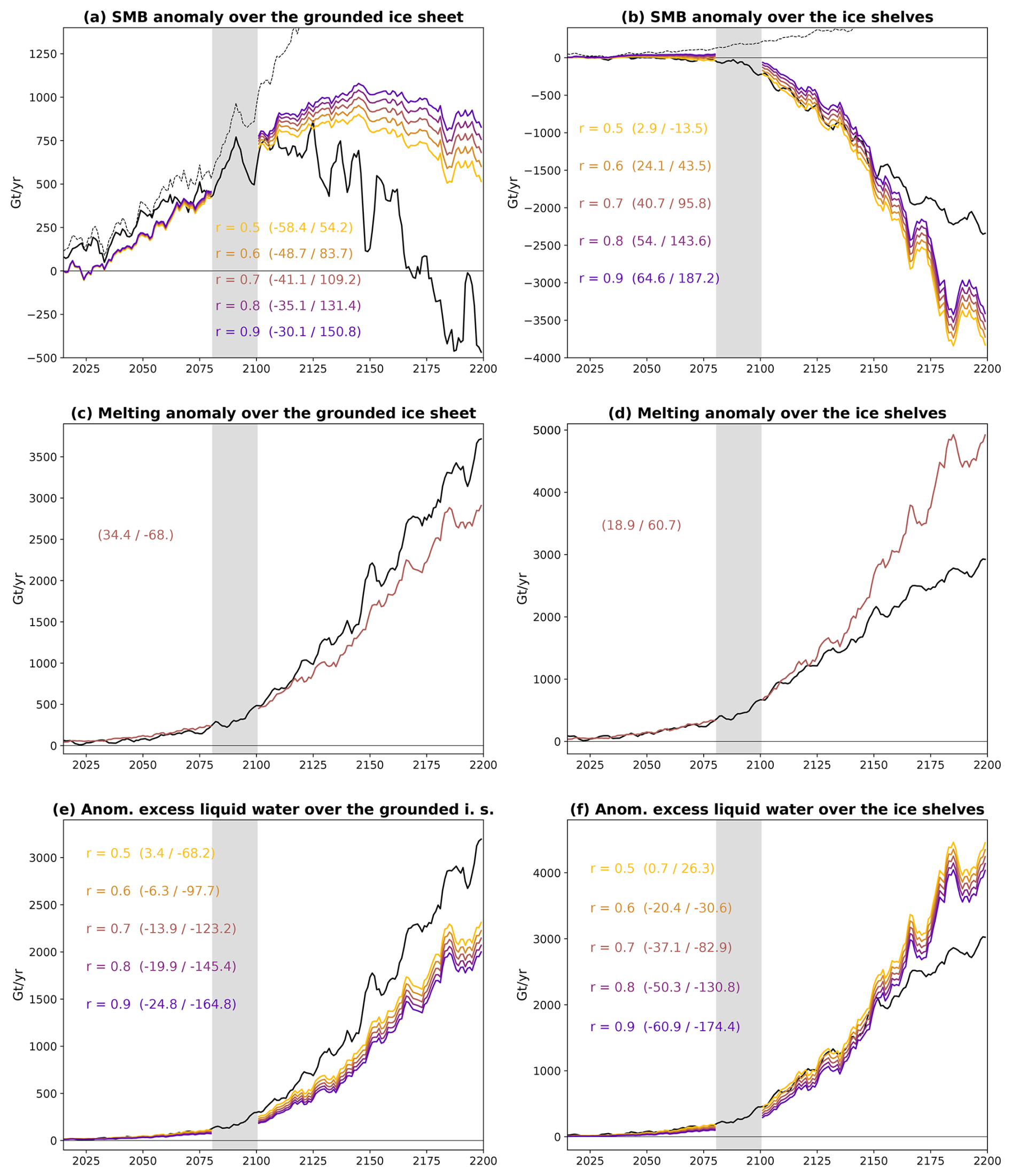
Figure 2 Evaluation of the emulation from another period (Fig. 1a) over the grounded ice sheet (a, c, e) and over the ice shelves (b, d, f) for SMB (a, b), surface melting (c, d), and production of liquid water beyond firn saturation (e, f). The solid black lines show the original MAR–IPSL-CM6A-LR simulation. The coloured lines are the emulations from the 2081–2100 period (shaded in grey), both backward in time (left side of the grey area) and forward in time (right side of the grey area). The emulation is shown for several values of r (see Eq. 4), and the bias values are indicated for both 2061–2080 (20-year backward emulation) and 2101–2120 (20-year forward emulation). The dashed black lines in panels (a) and (b) show the SMB directly calculated from the IPSL-CM6A-LR outputs following the ISMIP6 approach (Nowicki et al., 2020, their Appendix C). The anomalies are calculated with respect to the 1995–2014 mean. The time series on this plot are filtered through a 5-year running average.

The emulation backward to pre-2081, i.e. toward a colder climate, is less biased than the emulation forward to post-2100, i.e. toward a warmer climate (Fig. 2). Over the grounded ice sheet, the forward-emulated SMB has biases that remain small over the first 10 years and reasonable (∼ 10 %) over the first 20 years for r=0.5 and r=0.6. However, the forward emulation fails to represent SMB after 2120 due to a significantly underestimated runoff. This is largely due to the inability of our emulation method to initiate melting at locations that never experienced melting over 2081–2100. The backward emulation over the grounded ice sheet is quite accurate for the first 20 years, i.e. for moderate changes in climate conditions, and is moderately low-biased back to 2015.

Over the ice shelves, the emulation forward is accurate in the first 50 years (Fig. 2b, d, f). The best results over this first period are obtained for r=0.50 and r=0.60. After 2150, melt rates in the original MAR simulation start increasing more linearly with time, and our emulation overestimates melt rates and therefore mass loss. This is likely due to feedbacks that are represented in the MAR simulations but not in the IPSL-CM6A-LR model or in our emulation method. Indeed, the appearance of bare ice and changes in the cloud radiative properties have a strong impact on the projected SMB over Greenland (Hofer et al., 2020; Mostue et al., 2024), and a similar effect was found in warmer conditions in Antarctica (Kittel et al., 2022). For a CMIP model like IPSL-CM6A-LR that fails to represent meltwater runoff, our emulation method toward a warmer climate is nonetheless preferable to directly estimating the SMB from CMIP model outputs (see dashed black lines in Fig. 2a, b).

From this first evaluation, we conclude that our emulation method is suitable for the extension of RCM simulations into a warmer future for a maximum of 20 years over the grounded ice sheet and 50 years over the ice shelves. The extension to colder conditions in the past is more accurate as our emulation method is more suitable for reducing melt rates than for creating new melting areas. In the following, we use r=0.60 as it fits well the original simulation while remaining within the range of previous studies. The spatial patterns are also well represented by this method (Appendix D, Fig. D1).

2.3.4 Emulation from another scenario

We now assess the ability of our method to emulate several scenarios from a MAR simulation driven by a warmer scenario (Fig. 1b). As mentioned previously, our method is not able to create new melting areas, but it is well suited to decrease melt rates in colder conditions. We therefore consider the three MAR simulations for which we have the SSP1-2.6, SSP2-4.5, and SSP5-8.5 scenarios (MAR–CESM2, and MAR–UKESM1-0-LL, MAR–MPI-ESM1-2-HR), and we evaluate the emulation of both SSP1-2.6 and SSP2-4.5 from SSP5-8.5. The calculations are done separately for each of the corresponding simulations (based on the parameters in Table C1), but the results are presented in Fig. 3 as averages over the three CMIP models.

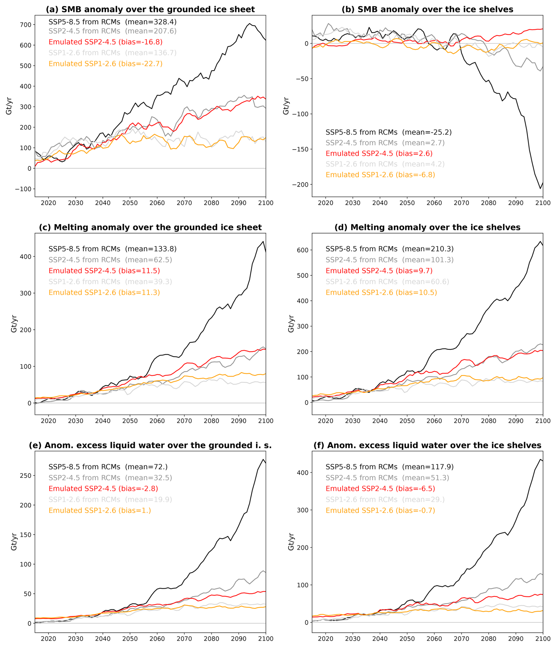
Figure 3 Evaluation of the emulation from a warmer scenario (Fig. 1b) over the grounded ice sheet (a, c, e) and over the ice shelves (b, d, f) for SMB (a, b), surface melting (c, d), and production of liquid water beyond firn saturation (e, f). The black and grey lines show the original MAR simulations, while the coloured lines correspond to the emulated SSP1-2.6 and SSP2-4.5 scenarios based on the SSP5-8.5 MAR simulation and the CMIP near-surface air temperatures. Every line on this plot is the average of three simulations or emulations: MAR–CESM2, MAR–UKESM1-0-LL, and MAR–MPI-ESM1-2-HR. The anomalies are calculated with respect to the 1995–2014 mean. The time series are filtered through a 5-year running average. The mean and biases over 2015–2100 are indicated on each panel.

Similarly to the previous subsection, each emulated year is the average of 20 emulations from a reference ranging from 10 years before to 9 years after the emulated year (Fig. 1b). Doing so, the interannual variability in the extended variables is only attributed to the air temperature variability in the corresponding scenario.

The SSP1-2.6 and SSP2-4.5 emulated fields are quite accurate over the grounded ice sheet during the 21st century: the biases indicated in Fig. 3 for the emulated values are relatively low compared to the mean values simulated by MAR. The bias in emulated runoff becomes larger at the end of the 21st century in the SSP2-4.5 scenario (Fig. 3e–f). This bias has little impact on the grounded ice sheet SMB (Fig. 3a) but cancels the small negative SMB anomaly simulated over the ice shelves near 2100 (Fig. 3b). These biases are small and limited to the end of the 21st century, so we conclude that our method is suitable for the emulation of multiple SSP scenarios based on an existing MAR simulation in a warmer scenario (here SSP5-8.5). The spatial patterns are also well represented by this method (Appendix D, Fig. D2).

2.3.5 Emulation from other CMIP models

Here we assess the ability of our method to emulate MAR simulations driven by other CMIP models (Fig. 1c). We consider five MAR simulations driven by different CMIP models under either SSP5-8.5 or RCP8.5, which have a similar radiative forcing. We assess the emulation from the same simulation (for verification of our method) and from six MAR simulations driven by other CMIP models. We use a similar methodology as in the previous subsection, calculating the average emulation of every year from 20 reference years (Fig. 1c), but instead of using the actual temperature as in the two previous subsections, we use the temperature anomaly with respect to each model's climatology. This was needed given that typical values of near-surface air temperature may vary from one CMIP model to another, in particular due to differences in the first level height and in their ability to represent stable surface boundary layers over ice sheets.

The method is evaluated in Fig. 4. First of all, the minimal differences between the black dots on each radial and the coloured dot corresponding to the same climate model show that the biases are small for MAR simulations derived from themselves. This shows that our methodology and its implementation are robust. We nonetheless note larger differences between the black dots on each radial and the coloured dots corresponding to the other climate models in Fig. 4c, d, indicating significant biases in melt rates when a MAR simulation is derived from another one. This alters the emulated SMB (Fig. 4a, b). MAR–ACCESS1.3 is an outlier and leads to melt emulation with the largest biases for the four other models. The realistic SMB emulations derived from MAR–ACCESS1.3 are mostly compensations between overestimated melt (Fig. 4c, d) and overestimated accumulation. The other CMIP5 simulation, MAR–NorESM1-M, is closer to the CMIP6 simulations even if the SMB is generally overestimated over the grounded ice sheet. The CMIP5 models have a relatively low ECS, and starting from MAR forced by any of these CMIP5 models does not give good emulations of models like CESM2 or CNRM-CM6-1 that both experience particularly strong warming over the 21st century (Kittel et al., 2021, 2022).

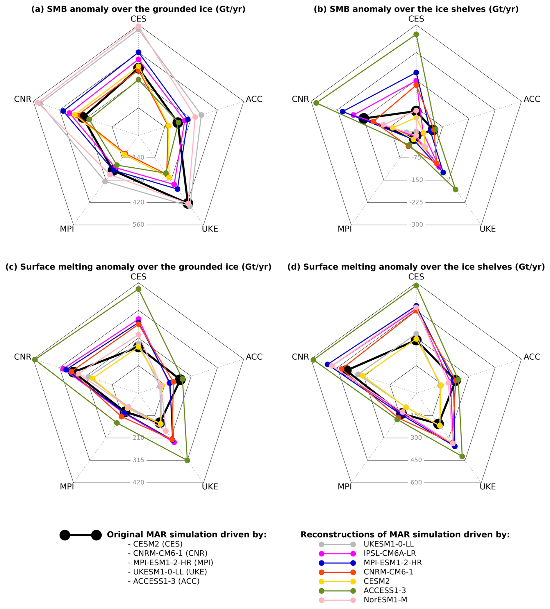
Figure 4 Evaluation of the emulation from other CMIP models (Fig. 1c) for SMB (a, b) and surface melting (c, d). The five radial lines correspond to five original MAR simulations driven by different CMIP6 or CMIP5 models, with the radial distance (thick black dots) indicating the SMB or melt rate values. The coloured dots correspond to the emulated values from surface temperatures of another CMIP model. The black and coloured pentagons link the dots for a better overview. The thin grey pentagons indicate the SMB or melt rate isovalues. The anomalies are calculated over 2015–2100 with respect to 1995–2014 under the SSP5-8.5 or RCP8.5 scenarios.

Given the biases of the emulation from a single model, we now assess the average of five emulations from different MAR simulations (excluding the simulation itself and the MAR–ACCESS1.3 outlier). The emulation is made for three SSP scenarios based on the five MAR simulations under the same scenario if available or SSP5-8.5 otherwise. For clarity, we present the average results for MAR–CESM2, MAR–UKESM1-0-LL, and MAR–MPI-ESM1-2-HR, which are the three MAR simulations for which we have all three scenarios (Fig. 5).

Averaging the emulation from several MAR simulations clearly improves the results, and the emulated SMB is generally quite accurate throughout the 21st century (Fig. 5a, b), although the mass loss at the surface of ice shelves is overestimated under SSP5-8.5 due to overestimated melt and runoff (Fig. 5d, f). Decreasing the r value would reduce the runoff bias here, but changing the r value would neither be consistent with the results of the previous sections nor reflect physical processes.

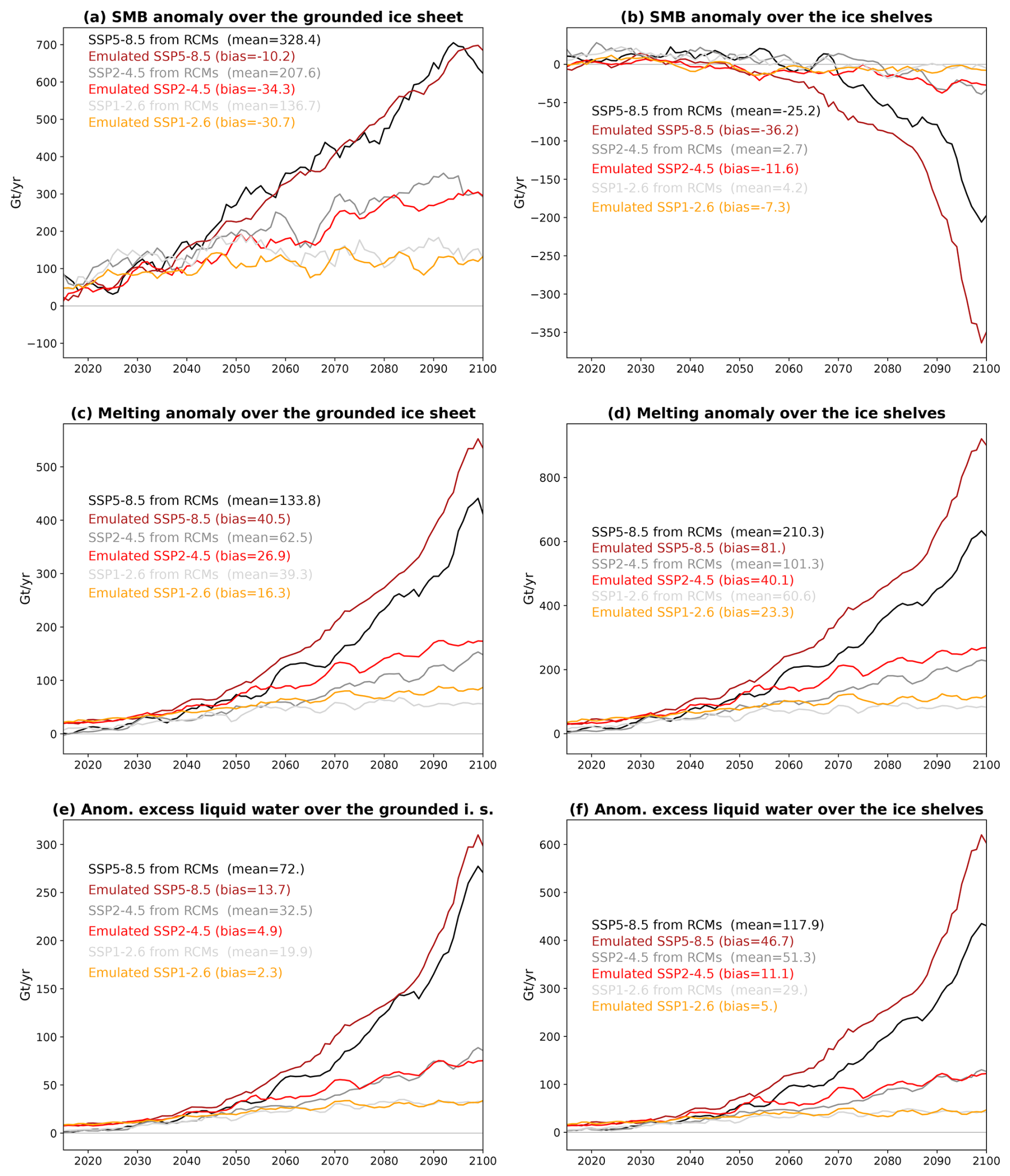
Figure 5 Evaluation of the emulation from five other CMIP models (Fig. 1c) over the grounded ice sheet (a, c, e) and over the ice shelves (b, d, f) for SMB (a, b), surface melting (c, d), and production of liquid water beyond firn saturation (e, f). The black and grey lines show the original MAR simulations for three SSP scenarios, while the coloured lines correspond to the emulation of these simulations from five independent models. Every line on this plot is the average of three simulations or emulations: MAR–CESM2, MAR–UKESM1-0-LL, and MAR–MPI-ESM1-2-HR. The anomalies are calculated with respect to the 1995–2014 mean. The time series are filtered through a 5-year running average. The mean and biases over 2015-2100 are indicated on each panel.

From this evaluation, we conclude that our multi-model emulation method is suitable for the emulation of MAR simulations driven by CMIP models that have never actually been used to drive MAR simulations. The spatial patterns are also well represented by this method (Appendix D, Fig. D3). It is important to stress that this method only gives meaningful results because of the average over several CMIP models, possibly due to the various responses of clouds and snow albedo from one model to another for a given warming level (Kittel et al., 2022).

2.4 Method used to build the ensemble of projections

Here we explain how we combine the three types of emulations summarized in Fig. 1 and how we weight the CMIP models to build our ensemble of projections. Then we explain how the liquid water beyond firn saturation is used in the SMB calculation and to estimate the potential for ice shelf hydrofracturing.

First, when the SSP5-8.5 MAR simulation driven by a given CMIP model is available but not the other scenarios, we emulate the SSP2-4.5 and SSP1-2.6 scenarios from SSP5-8.5 (blue curve in Fig. 6a). If MAR has not been driven at all by a given CMIP model, we emulate all scenarios from six MAR simulations driven by six CMIP models, taking the closest available scenario of a given model if several are available (see 1980–2100 in Fig. 6b). We then emulate the historical period from 1850 to 1979 for all models based on the 1980–1999 period, which is the earliest period covered by the MAR simulations (grey curves in Fig. 6). For this, we use the method for emulating from another period (Fig. 1a).

For the projections between 2101 and 2200, we have a single MAR simulation forced by IPSL-CM6A-LR under SSP5-8.5 due to the non availability of 6-hourly 3-dimensional atmospheric data beyond 2100 for most CMIP models. The CMIP near-surface air temperatures are nonetheless available until 2200 for seven other simulations for both SSP1-2.6 and SSP5-8.5 (see stars in Table 1). For these seven simulations, we emulate the 22nd century based on the CMIP model temperatures and the MAR–IPSL-CM6A-LR simulation (see 2121–2200 in Fig. 6b). To ensure some continuity around 2100 and to benefit from better emulations before 2100, we apply a 20-year ramping transition (yellow area in Fig. 6b) over which we use a linear combination of the emulation from the 2081–2100 period and the emulation from MAR–IPSL-CM6A-LR. For the emulation of MAR–UKESM1-0-LL after 2100, we use the ensemble member r4i1p1f2 instead of r1i1p1f2 in the actual MAR simulations because this is the only one available beyond 2100.

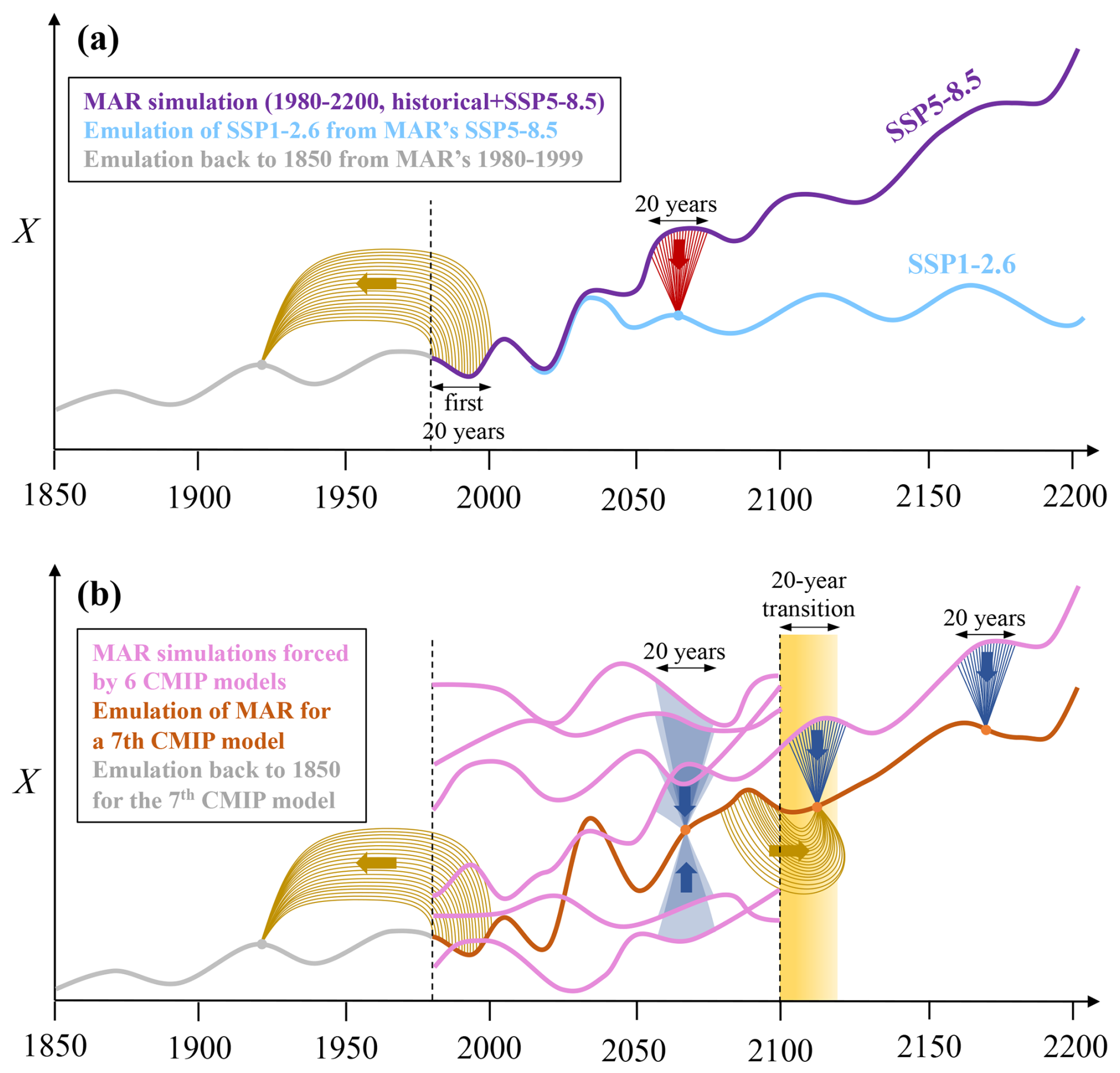
Figure 6 Schematic of the methods used to build our ensemble of projections. (a) A MAR simulation from 1980 to 2200 under SSP5-8.5 is used to obtain SSP1-2.6. (b) Six MAR simulations forced by six different CMIP models from 1980 to 2100 under a given scenario are used to emulate the corresponding MAR simulation for a seventh CMIP model. The methods are described in Sect. 2, and the colours used to represent the emulation methods are the same as in Fig. 1. Variable X represents either SMB minus runoff or the surface melt rate.

The median ECS of this 16-model ensemble is 4.2 °C, and the ECS of 3 models out of 16 exceeds 5.0 °C, which is high compared to the best estimate of 3.0 °C and the 90 % confidence interval of 2.0–5.0 °C estimated in the IPCC Sixth Assessment Report (Forster et al., 2021). To build a realistic ensemble mean, we therefore attribute weights to individual models, which are the probability of a skew-normal distribution fitted to obtain the 5th, 50th, and 95th percentiles at ECS of 2.0, 3.0, and 5.0 °C (Fig. 7). The corresponding weights are listed in Table 1. Despite the imperfect model sampling, the weighted 16-model mean ECS falls from 4.0 to 3.3 °C thanks to weighting, which is closer to the best ECS estimates (Forster et al., 2021) and to the CMIP5 multi-model mean (3.2 °C in Meehl et al., 2020). To calculate the percentiles of the weighted distribution, we consider a number of values equal to 100 times the weight for each model, which shifts the multi-model ECS distribution much closer to the ECS very likely range (see small triangles in Fig. 7). We keep the same weights for the ensemble until 2200 even though the 8-model sampling is not as good as a 16-model sampling, giving an ECS weighted mean of 3.7 °C (versus 4.4 °C for the unweighted mean).

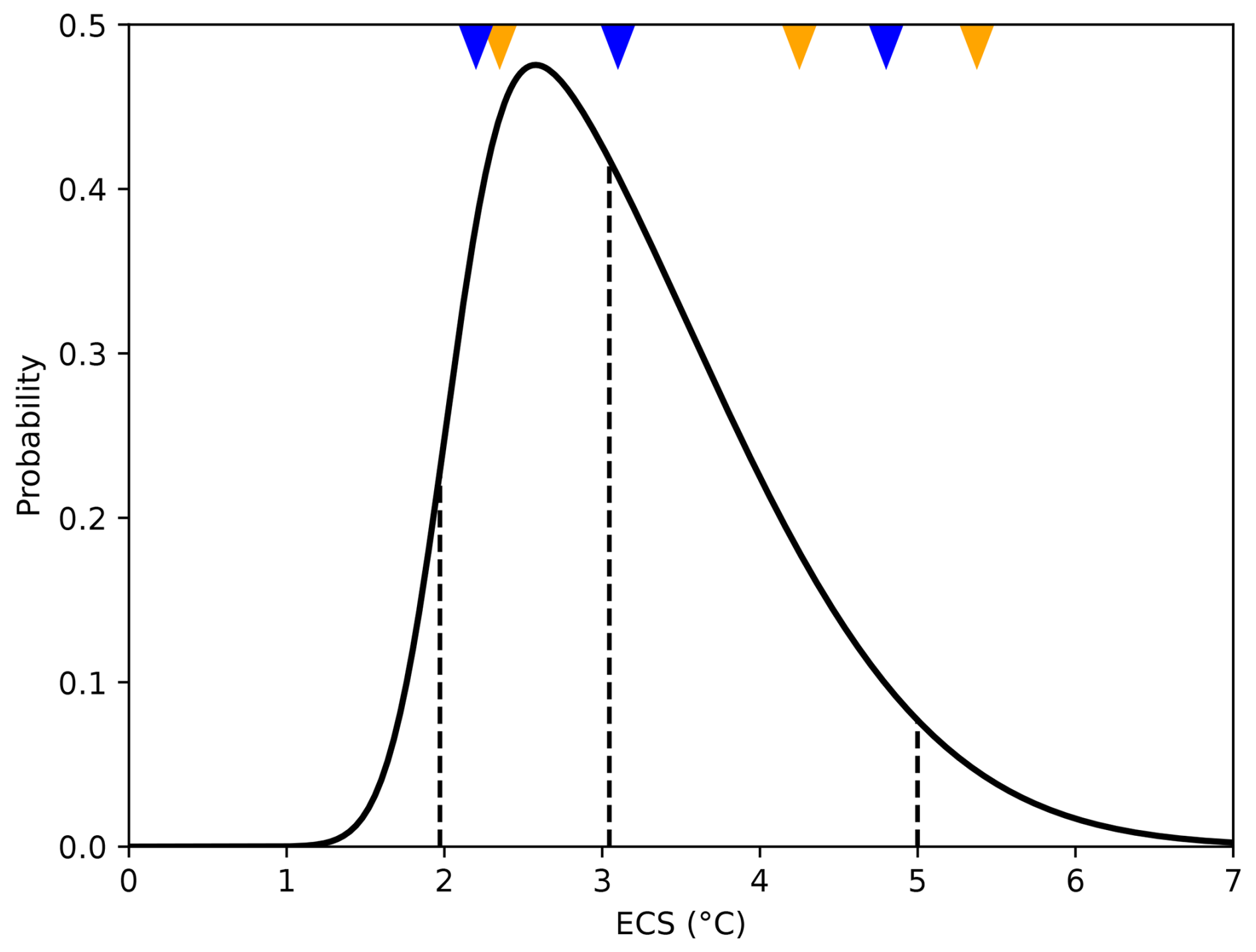
Figure 7 Skew-normal ECS probability (solid line) fitted to obtain its 5th, 50th, and 95th percentiles at 2.0, 3.0, and 5.0 °C (dashed lines). The orange triangles indicate the 5th, 50th, and 95th percentiles of the ECS of the unweighted 16-CMIP-model distribution, and the blue triangles show the equivalent for the weighted distribution. The skew-normal distribution was generated using the skewnorm.pdf function of the scipy.stats package (Virtanen et al., 2020), with a skewness parameter of 5.08, an offset parameter (loc) of 2.02 °C, and a scale parameter of 1.52.

In the next section, we first use our methodology to estimate the SMB contribution to changes in sea level. As we see in the next section, very warm conditions may lead to runoff production over the grounded ice sheet up to elevations of 1000 m above sea level, and a large part of the meltwater not retained in the firn is expected to drain onto ice shelves located downstream (Kingslake et al., 2017). We therefore assume that all excess liquid water over the grounded ice sheet flows to the ice shelves downstream or directly into the ocean. Therefore, as far as the grounded ice sheet is concerned, the production of liquid water beyond firn saturation is considered runoff, i.e. a negative term in our SMB calculations.

We then use our methodology to estimate when the surface conditions have the potential to trigger ice shelf hydrofracturing. As discussed previously, melt rates can be too low to saturate the firn with liquid water, which is why we consider that a necessary condition for hydrofracturing has to be based on the production of excess liquid water and not on melt rates as done in previous studies (e.g. Trusel et al., 2015; Nowicki et al., 2020; Seroussi et al., 2020). The relatively flat ice shelves are treated in a different way than the grounded ice. Indeed, in addition to the liquid water produced locally, the ice shelves receive the liquid water that was produced beyond firn saturation over the upstream grounded ice sheet. To account for this, we assume that an ice shelf receives a fraction of the liquid water produced over the grounded ice of its drainage basin. The fraction is taken to be the fraction of the basin coastline occupied by the ice shelf.

Another specificity of ice shelves is that they are relatively flat and can bend, so it is impossible to estimate the amount of liquid water forming ponds or flowing into the ocean without a dedicated hydrology–firn–ice shelf model. This is why we introduce an empirical threshold on the production rate of excess liquid water to assess the potential for hydrofracturing. The idea is to have a rate that is sufficiently high to form ponds and fill crevasses even if a part flows into the ocean. The average production of excess liquid water over Larsen B prior to its collapse was estimated to be between 200 and 300 $\mathrm{kg}{\mathrm{m}}^{-\mathrm{2}}{\mathrm{yr}}^{-\mathrm{1}}$ (Holland et al., 2011; van Wessem et al., 2016; Costi et al., 2018), so our threshold has to be lower than that. There is nonetheless a large uncertainty in the threshold, and we sample it in a normal distribution of 150 and 61 $\mathrm{kg}{\mathrm{m}}^{-\mathrm{2}}{\mathrm{yr}}^{-\mathrm{1}}$ of mean and standard deviation, respectively. This is chosen to obtain 90 % of the threshold values between 50 and 250 $\mathrm{kg}{\mathrm{m}}^{-\mathrm{2}}{\mathrm{yr}}^{-\mathrm{1}}$. The lower end of this range is chosen empirically so that not too many ice shelves are above the threshold in present-day conditions. The uncertainty in the threshold is hence included in the calculation of the probability of a given ice shelf being over the threshold.

In the next section, we present our results as confidence intervals, which we define as in the IPCC reports: 17th–83rd percentiles for the likely range (66 % probability) and 5th–95th percentiles for the very likely range (90 % probability). These percentiles account for the uncertainty of the CMIP models weighted to account for the likelihood of their ECS and for the uncertainty in the threshold of liquid water production in excess when we investigate the potential for ice shelf hydrofracturing.

3 Ensemble of projections from 1850 to 2200

Here we use the emulated ensemble to estimate the SMB evolution over the grounded ice sheet from 1850 to 2200 and the equivalent changes in sea level (Sect. 3.1) as well as the production of excess liquid water from 1850 to 2200 and the implications for ice shelf hydrofracturing (Sect. 3.2). Importantly, our estimates of sea level projections only contain the part related to SMB variations and not the contribution from the ice sheet dynamics, which is driven by ocean-induced melting and hydrofracturing. In Appendix E, we also describe the SMB evolution over ice shelves.

3.1 Grounded ice sheet and sea level

First of all, our emulated ensemble indicates that the grounded ice sheet SMB was 110 Gt yr⁻¹ lower in 1850–1869 than in 1995–2014 and increased slowly through the 20th century (Fig. 8). In comparison, a combination of ice cores and simulations from another regional climate model gave ∼ 200 Gt yr⁻¹ of difference between these two periods (Thomas et al., 2017). This increasing SMB in our emulation is equivalent to a reduction of 1.3 cm of global mean sea level from 1900 to 2010 (likely range of 0.4 to 2.2 cm) with respect to the 1891–1910 mean (i.e. assuming that the climatological SMB over 1891–1910 contributed to zero sea level rise).

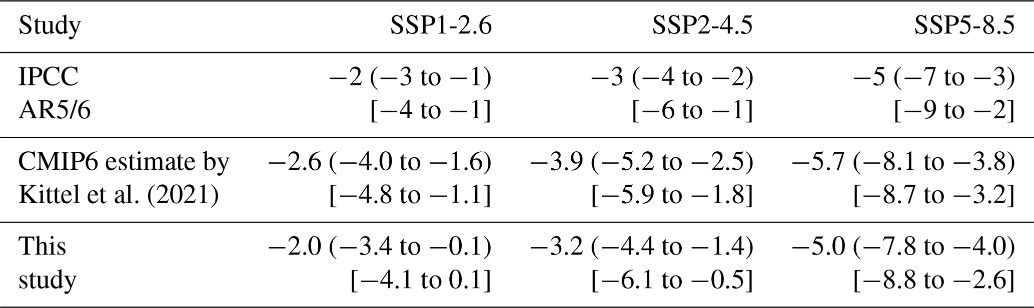
Our projections over grounded ice until 2100 agree quite well with previous estimates of sea level contribution reported by the IPCC for the three scenarios and are slightly lower than previous estimates for the unweighted CMIP6 ensemble (Table 3). We estimate a median SMB mitigation of sea level rise between 2.0 and 5.0 cm depending on the scenario. As in Kittel et al. (2021), the three SSP scenarios diverge after 2040: the SSP1-2.6 SMB remains ∼ 100 Gt yr⁻¹ above 1995–2014, the SSP2-4.5 SMB keeps increasing until 2100 at a rate similar to 1970–2014, and the SSP5-8.5 SMB increases 1.7 times faster than SSP2-4.5 until 2100 (Fig. 8).

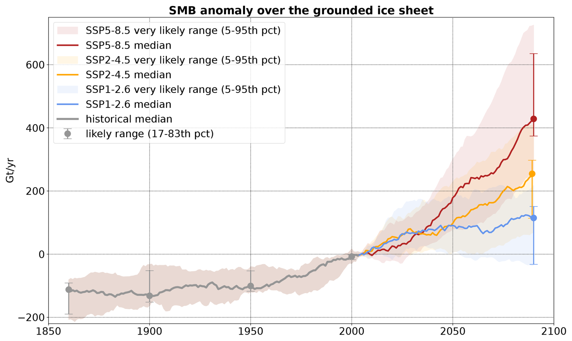
Figure 8 Emulated ensemble of surface mass balance over the grounded Antarctic Ice Sheet for the historical period and three SSP scenarios. The median and percentiles are calculated based on the 16-model ensemble weighted to match with the very likely range of ECS (see Sect. 2.1). A 21-year running average has been used for all the time series.

Kittel et al. (2021)

Table 3 Projected sea level contributions (in cm) from the Antarctic Ice Sheet SMB from 2000 to 2099 (relative to 1995–2014, i.e. assuming that the mean SMB over that period yields no sea level rise), for the three selected SSP scenarios, shown as the median, likely range, i.e. 17th–83rd percentile, in parentheses and very likely range, i.e. 5th–95th percentile, in square brackets. The IPCC-AR5/6 estimates are those presented in Table 9.3 of IPCC-AR6 (Fox-Kemper et al., 2021), i.e. recalculated for the SSP scenarios from IPCC-AR5, and originally derived from the CMIP5 global mean surface air temperature using a linear accumulation–temperature relationship (Church et al., 2013). The data of Kittel et al. (2021) are statistical reconstructions based on the air temperature averaged south of 60° S for 33 CMIP6 models, and the percentiles have been recalculated for this table.

For seven out of eight models going beyond 2100, the maximum SMB over the grounded ice sheet is reached between 2090 and 2120 under SSP5-8.5 and a few decades earlier under SSP1-2.6 (Fig. 9). Under SSP1-2.6, the SMB over the grounded ice sheet goes back to present-day values during the 22nd century. Under SSP5-8.5, the three models with an ECS lower than 4 °C predict an SMB that remains above the present-day value until 2200. In contrast, four models predict that the increase in runoff over the grounded ice sheet will overwhelm the increase in accumulation, with an SMB decreasing below the present-day value after 2035 to 2075 depending on the model. It cannot be ruled out that the grounded ice sheet reaches a net surface mass loss near 2200, although this is extremely unlikely given that the two models crossing or approaching this limit are above the 95th percentile at the end of the 21st century.

In terms of sea level, the net contribution of the Antarctic SMB over 2000–2200 is between −10 and −1 cm for SSP1-2.6 and between −33 and +6 cm for SSP5-8.5 (Table 4). Interestingly, the relative importance of sea level reduction between SSP1-2.6 and SSP5-8.5 is reversed for the two models producing the largest amount of runoff in the 22nd century (MAR–CanESM5 and MAR–CESM2-WACCM) compared to the other models. This is due to the massive runoff production over the grounded ice sheet after 2150 under SSP5-8.5 in these two models, which counterbalances the excess of accumulation before 2150 (Fig. 9). MAR–CanESM5 even has a net positive contribution to sea level rise over the 2 centuries under SSP5-8.5.

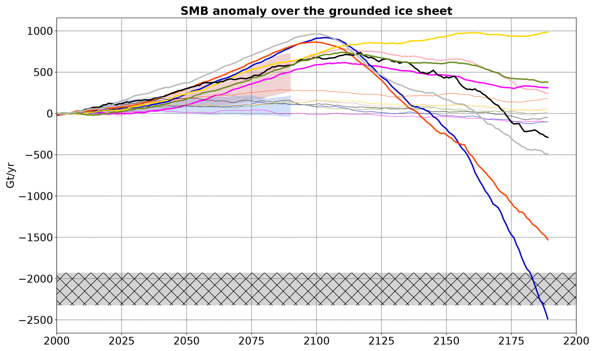
Figure 9 Eight emulations of surface mass balance over the grounded Antarctic Ice Sheet for the SSP-1.26 and SSP5-8.5 scenarios. The very likely range from 16 emulations over 2000–2100 (same as Fig. 8) is also shown. The hatched area indicates the anomaly interval at which SMB reaches zero according to the MAR, RACMO, and HIRHAM present-day values reported in Mottram et al. (2021). A 21-year running average has been used for all the time series.

In terms of patterns, the projected increase in SMB over the grounded ice sheet until 2100 is the largest along the coast of the Bellingshausen and Amundsen seas as well as in Dronning Maud Land (Fig. 10). The models producing large amounts of runoff by 2200 under SSP5-8.5 tend to have a lower SMB than presently below 1000 m above sea level, i.e. along the coastline and upstream of many ice shelves (Fig. 11).

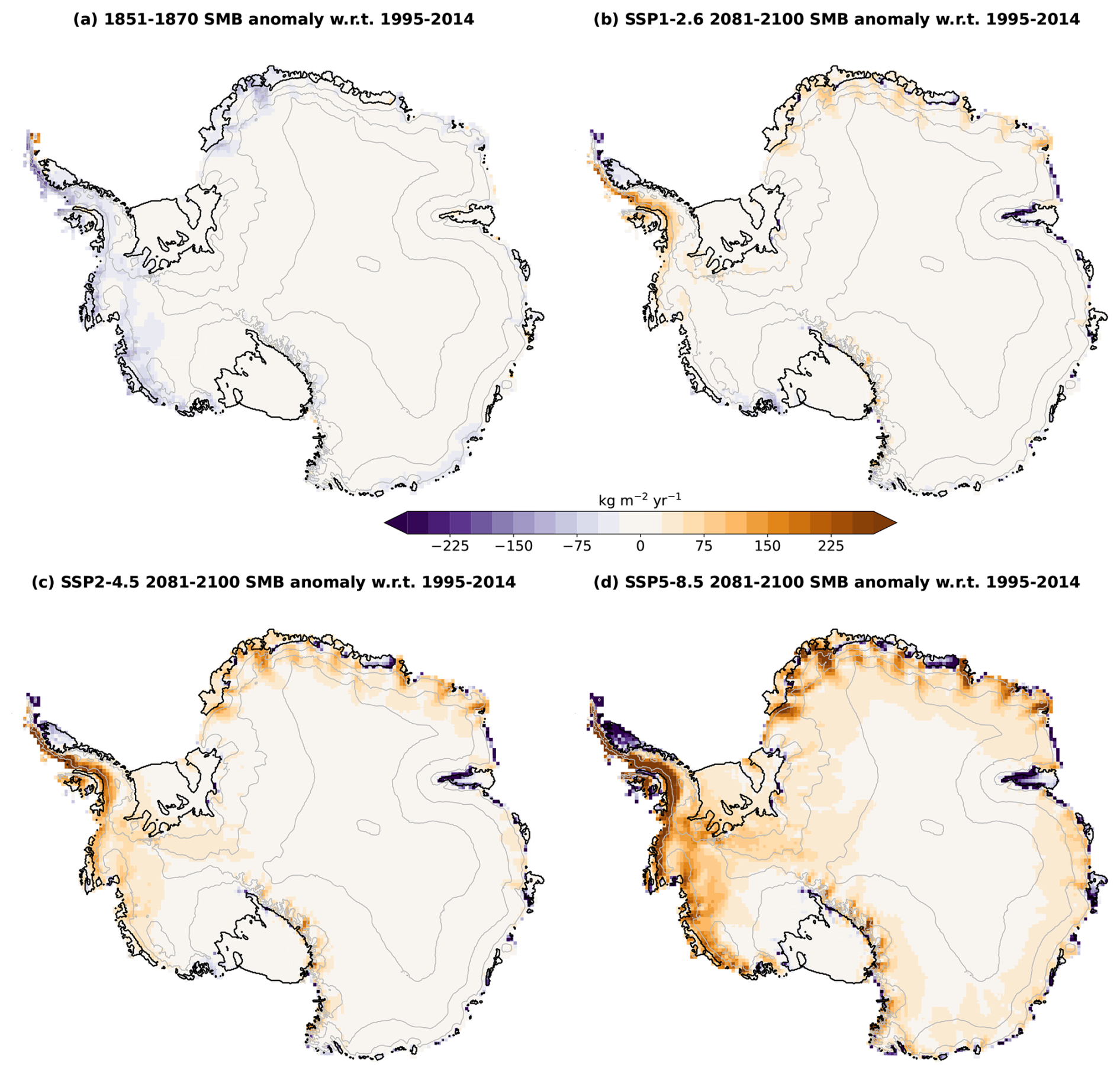
Figure 10 Weighted mean SMB anomaly for four different periods or scenarios with respect to the average SMB over 1995–2014. This was calculated from the 16 models listed in Table 1. The grey contours indicate the topography (every 1000 m), and the black contours show the ice shelves.

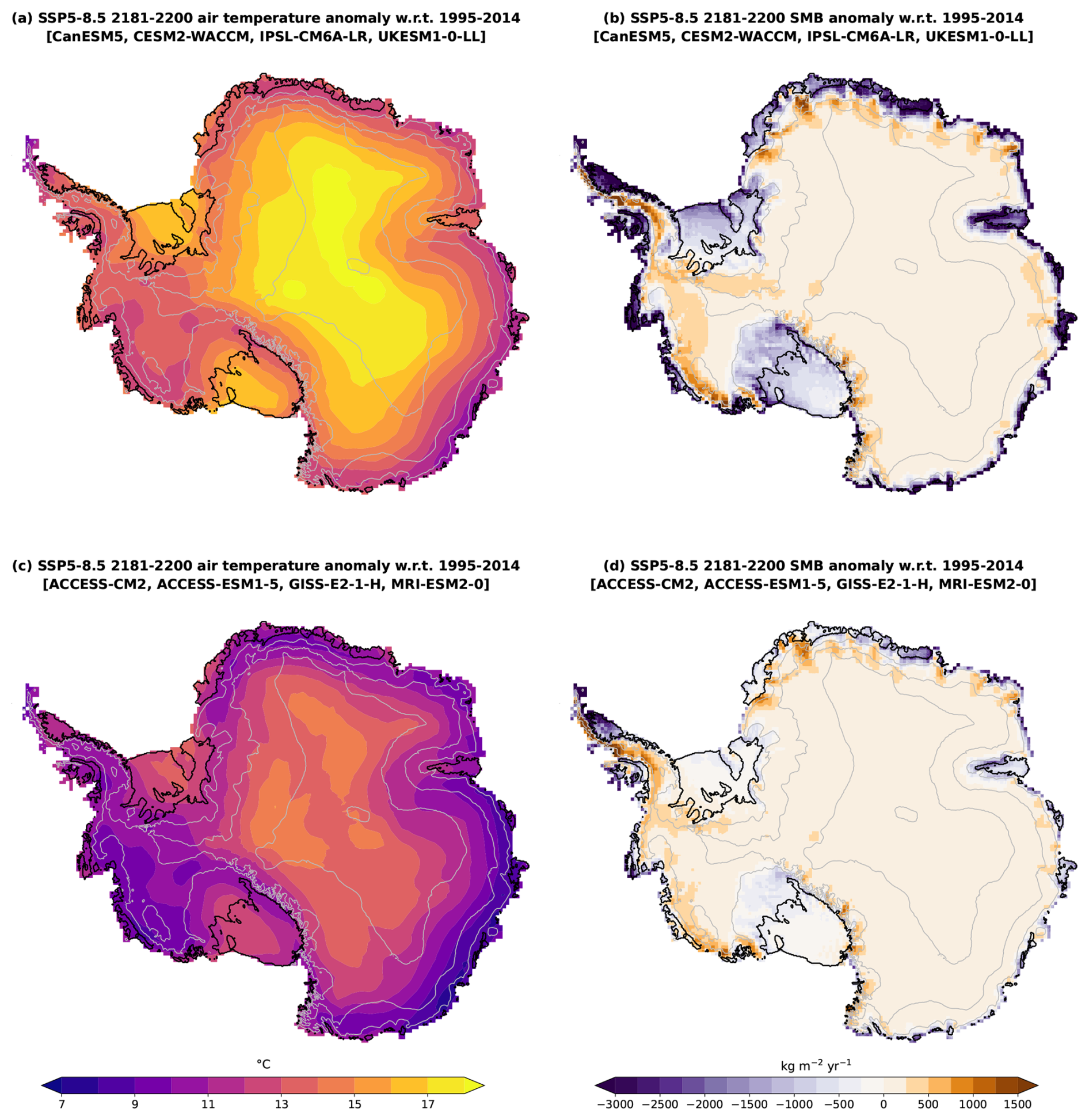
Figure 11 Mean 2181–2200 near-surface air temperature (a, c) and SMB (b, d) anomaly under SSP5-8.5 with respect to the 1995–2014 mean for the four models with the most negative SMB spatially integrated anomaly (a, b) and the four models with the least negative spatially integrated SMB anomaly (c, d). This was calculated from the eight models of Table 1 that are available until 2200, with equal weight for all models. The grey contours indicate the topography (every 1000 m), and the black contours show the ice shelves.

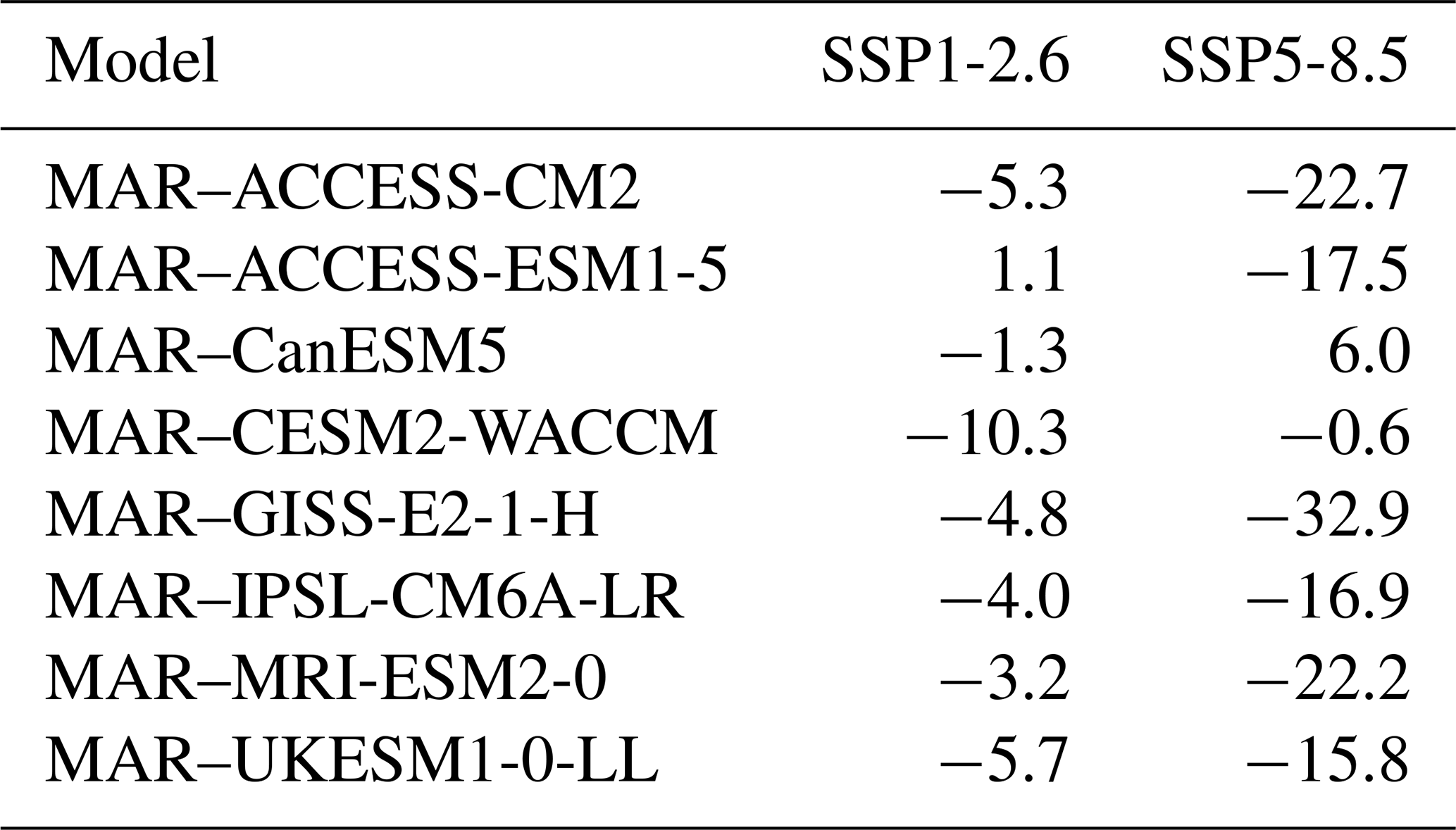
Table 4 Projected sea level contributions (in cm) from the Antarctic Ice Sheet SMB from 2000 to 2200 (relative to 1995–2014).

3.2 Ice shelves and hydrofracturing potential

We now investigate the years of emergence of surface conditions that make ice shelves prone to hydrofracturing, keeping in mind that mechanical conditions would also be necessary for the developments of fractures (see Introduction). As explained in Sect. 2.1, we use a threshold on the production rate of liquid water beyond firn saturation to identify such conditions.

According to our estimates, a few ice shelves were already likely (Fig. 12) or very likely (Fig. 13) in conditions favourable for hydrofracturing before 2015 and sometimes have been since the 19th century. This is the case of Larsen A and B that collapsed in 1995 and 2002 (Rott et al., 1996, 2002) after a progressive thinning that led to favourable mechanical conditions for fractures (Shepherd et al., 2003).

Further south in the Antarctic Peninsula, Larsen C, Wordie, and Wilkins have a likely range starting in the 1980s (Fig. 12) but extending toward the end of the 21st century. This considerable spread indicates present-day rates of liquid water production close to the threshold distribution. These three ice shelves are actually known for their recent evolution and wet surface conditions: the Wilkins Ice Shelf progressively thinned (Braun et al., 2009) before a partial disintegration in 2008 likely due to hydrofracturing (Scambos et al., 2009), the Wordie Ice Shelf progressively broke up from 1991 to 2009 (Doake and Vaughan, 1991; Cook and Vaughan, 2010), and the Larsen C Ice Shelf lost 25 %–30 % of its area from the 1970s to 2021 (Cook and Vaughan, 2010; Greene et al., 2022). Also in the Antarctic Peninsula, the George VI Ice Shelf has a likely range starting at the end of the 19th century. Melt ponds have been reported on George VI since the 1960s (Wager, 1972; Bell et al., 2018; Banwell et al., 2021), but the ice shelf compressive stress does not promote ice shelf fractures (LaBarbera and MacAyeal, 2011) even though the ice shelf lost 8 % of its area from 1947 to 2010 (Cook and Vaughan, 2010).

After the Antarctic Peninsula, the region where ice shelves are most prone to hydrofracturing in terms of surface conditions is the Indian Ocean sector of East Antarctica. The ice shelves in Vincennes Bay, East Antarctica, are estimated to be in similar surface conditions as Larsen A and B (Fig. 12). These ice shelves have been covered by supraglacial lakes (Arthur et al., 2020), and their extent has decreased by ∼ 10 % over the two first decades of the 21st century (Greene et al., 2022), but no widespread break-up has been observed so far. The Publications, Shackleton, and Moscow University ice shelves have a likely range starting before 2025, and widespread melt ponds or aquifers are observed in present-day conditions (Kingslake et al., 2017; Bell et al., 2018; Alley et al., 2018; Stokes et al., 2019; Arthur et al., 2020, 2022; Saunderson et al., 2022), again with no significant break-up reported recently. The Amery Ice Shelf, as well as Roi Baudouin and Nivl, further west in Dronning Maud Land, currently often covered with ponds or aquifers (Alley et al., 2018; Spergel et al., 2021; Arthur et al., 2022; Priya et al., 2024; Dell et al., 2024), have their likely range starting in ∼ 2050 for any scenario (Fig. 12).

The fate of the other ice shelves beyond 2050 is very much dependent on the emission scenario (Fig. 12). Under the SSP5-8.5 scenario, the number of ice shelves likely prone to hydrofracturing increases from 13±6 to all of the 56 considered ice shelves from 2050 to 2150. In contrast, this number only increases from 11±4 to 16±9 under SSP1-2.6, meaning that a majority of ice shelves are unlikely to experience hydrofracturing in this scenario. Under SSP2-4.5, we find that hydrofracturing conditions are likely not met before 2100 for 21 of the 56 considered ice shelves (Fig. 14).

The giant Ross and Ronne–Filchner ice shelves are unlikely to experience hydrofracturing before the early 22nd century in SSP5-8.5, consistently with previous studies (Kuipers Munneke et al., 2014; van Wessem et al., 2023; Dunmire et al., 2024; Veldhuijsen et al., 2024). In the Amundsen Sea, the ice shelves from Thwaites to Getz are also unlikely to experience hydrofracturing before the early 22nd century, consistently with the projections of Donat-Magnin et al. (2021) and with the little change in firn air content by 2100 reported by Dunmire et al. (2024) and Veldhuijsen et al. (2024).

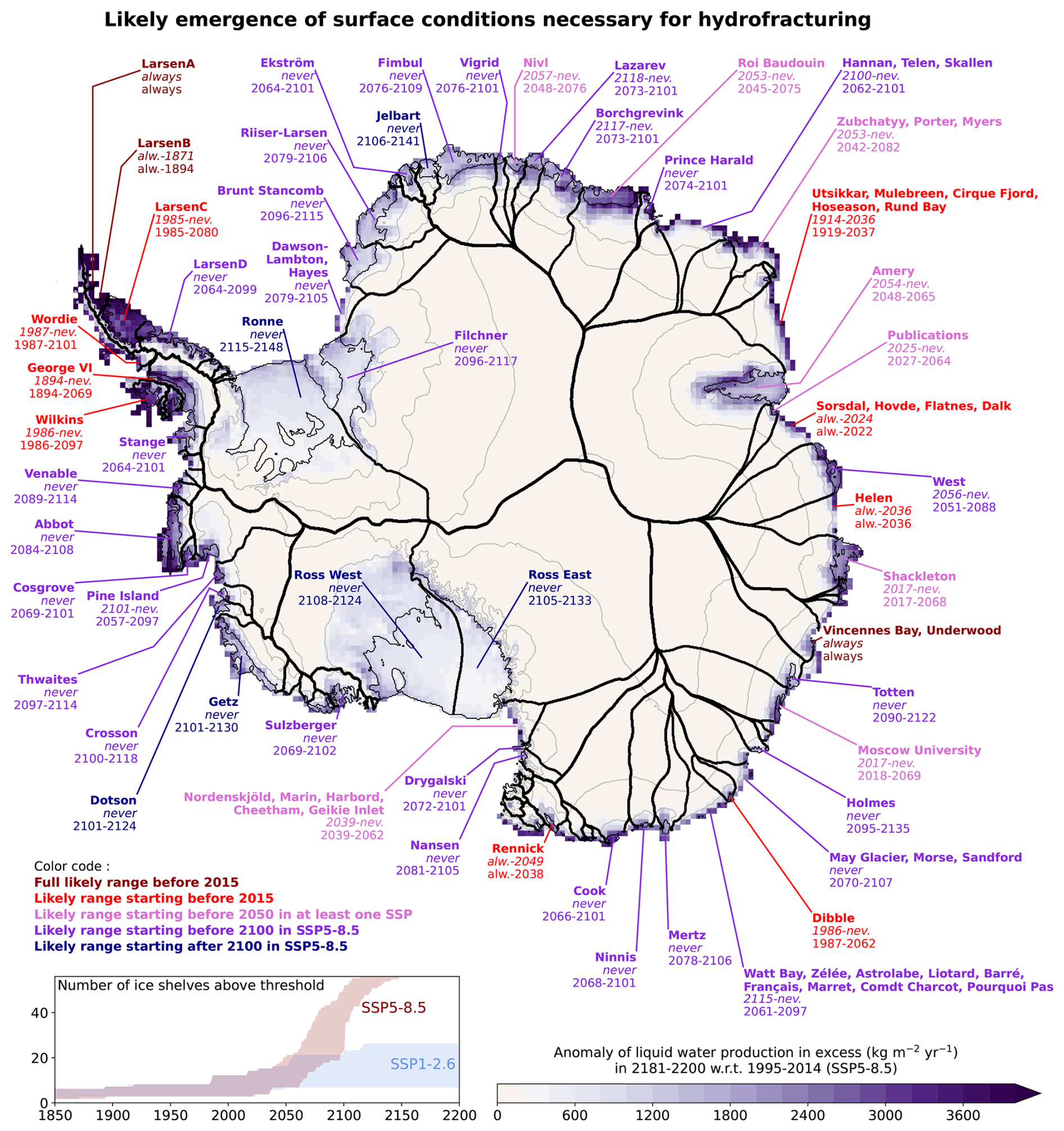
Figure 12 Time intervals at which the likely (17th–83rd percentiles) production of excess liquid water likely exceeds the threshold that makes hydrofracturing possible (see text) for 56 ice shelves or groups of ice shelves. The first time range, in italic, corresponds to SSP1-2.6, while the second range corresponds to SSP5-8.5. The estimated years are based on the weighted 16-model ensemble until 2100 and on the weighted 8-model ensemble from 2101 to 2200. Indications of “always” and “never” have to be understood as between 1850 and 2200 (e.g. never means either after 2200 or never). The background map shows the eight-model mean anomaly of liquid water production beyond firn saturation at the end of the 22nd century. The topography contours are in grey (every 1000 m), and the ice shelves are delineated in thin black. The contours of the drainage basins of individual ice shelves are drawn in thick black lines (from Mouginot et al., 2017, and Rignot et al., 2019).

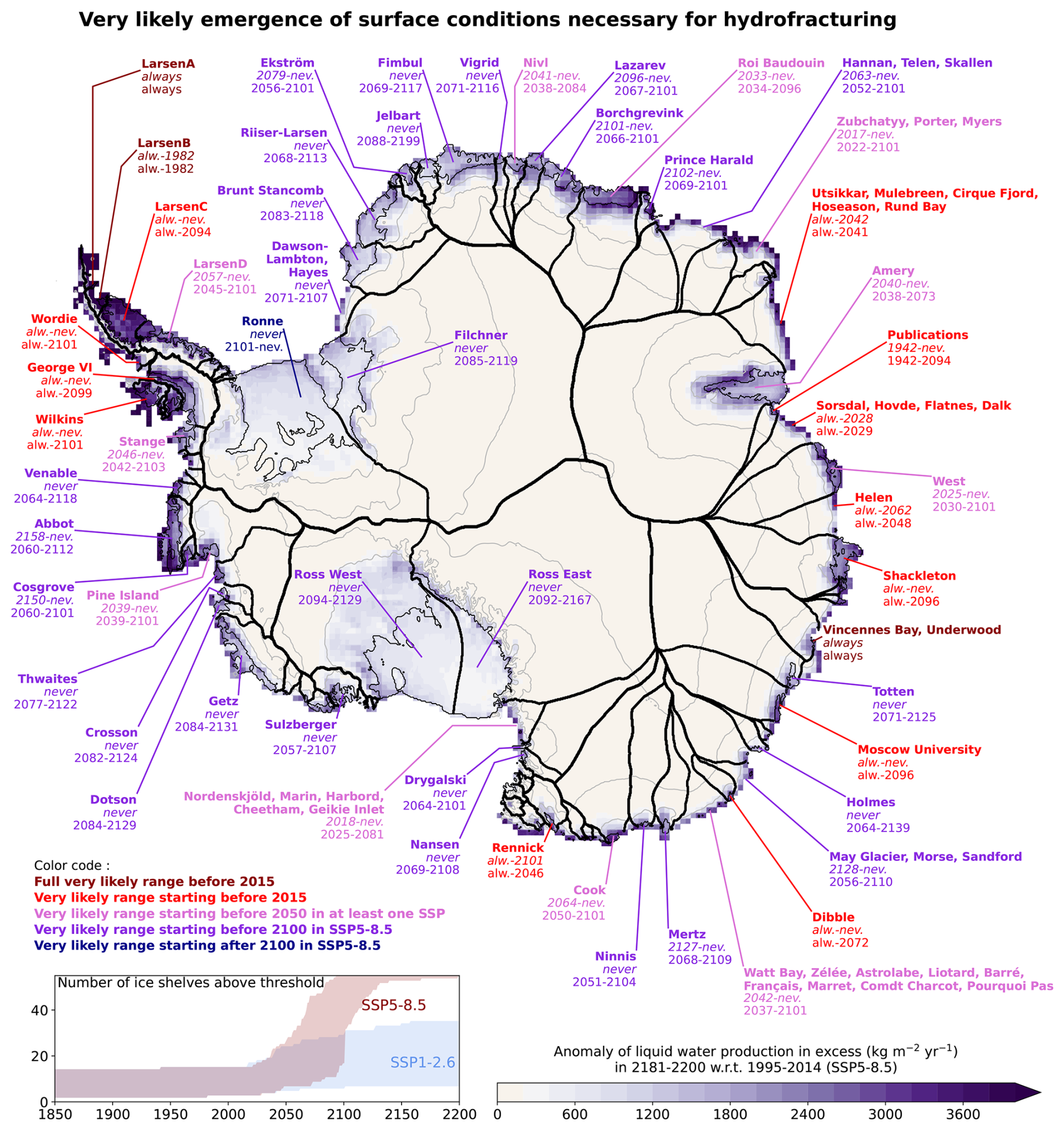
Figure 13 Same as Fig. 12 but for the very likely range (5th–95th percentiles).

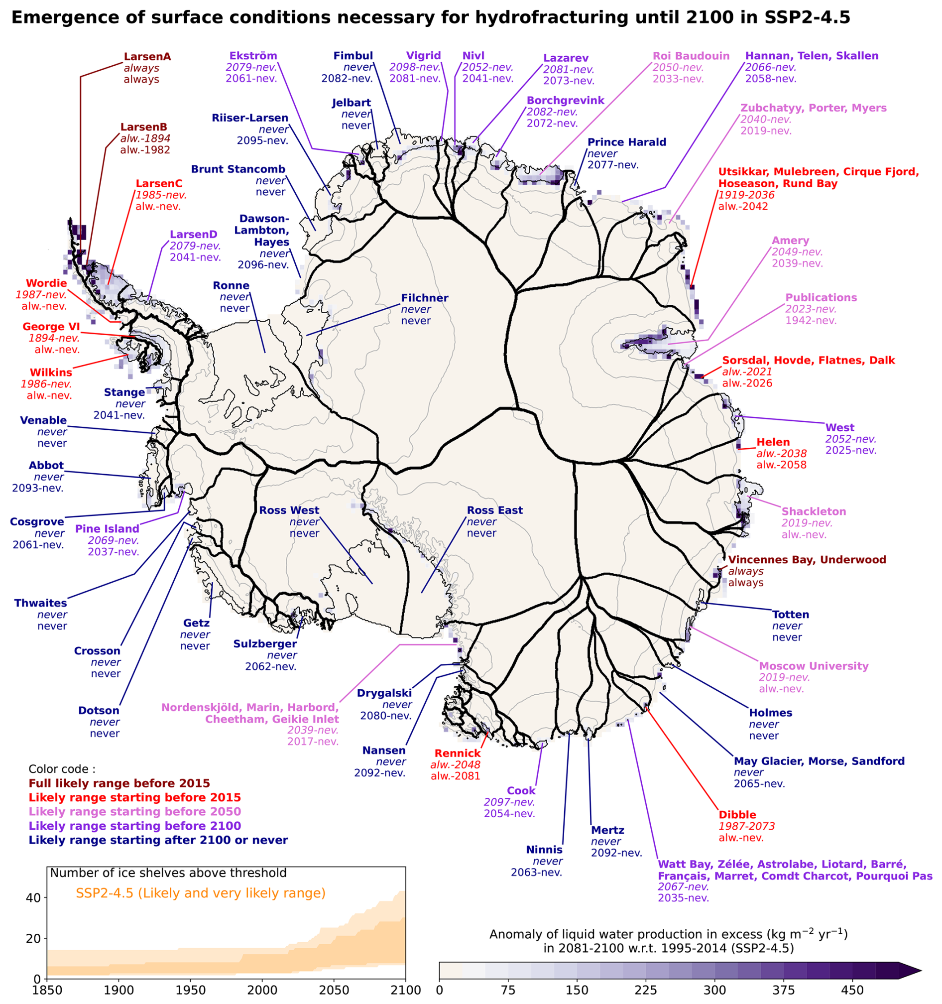
Figure 14 Similar to Fig. 12 but for the SSP2-4.5 scenario. The dates in italic give the likely range (17th–83rd percentiles), and the others give the very likely range (5th–95th percentiles). The background map shows the 16-model mean anomaly of liquid water production beyond firn saturation at the end of the 21st century under SSP2-4.5.

4 Discussion

In this study, we use a relatively simple model to emulate RCM simulations. It is based on exponential fits for snowmelt and accumulation rates. Although the method gives reasonably good results, we suggest that more complex fitting methods, in particular through deep learning algorithms fed by multiple CMIP model variables (e.g. Sellevold and Vizcaino, 2021; van der Meer et al., 2023), may improve our approach. A complex algorithm trained on regional climate simulations with complex physical parameterizations may be able to represent aspects that are not accounted for in our simple statistical–physical model, such as the emergence of bare ice and its effect on albedo, the presence of ice slabs in the firn, the effects of rainfall, the melt–elevation feedback, or the radiative feedbacks associated with the evolution of the cloud phase. Combining our methodology with a downscaling approach (e.g. Noël et al., 2023) may also improve the emulated data. For any method, the results presented in Sect. 2.3.5 stress the importance of using a training dataset made of RCM simulations driven by multiple CMIP models for obtaining robust results.

In this work, we also assume an instantaneous saturation of the firn beyond certain melt rates, while it can take an infinite amount of time to saturate it if melt rates are just above the threshold (e.g. Donat-Magnin et al., 2021). This could be addressed by introducing the temporal evolution of the depleted firn air volume in our simple model or in the deep learning approach or, in a simpler way, by introducing some time lag in the relationship between melt and firn saturation.

Our approach consists of emulating MAR simulations. Other RCMs, possibly combined with elaborated firn models, have similar skills in representing typical Antarctic conditions (Mottram et al., 2021), but there is a considerable spread in their response to surface warming (Glaude et al., 2024). For example, the depth and vertical resolution of firn models probably make important differences in the timing of runoff production. The 20 m firn layer simulated in MAR thus likely reaches liquid water saturation earlier than models with a thicker firn layer. One of the next priorities will therefore be to emulate the diversity of RCM or firn models sensitivities, which would make the uncertainty ranges much more comprehensive. The absence of physical representation of ponding and horizontal routing of liquid water nonetheless remains a major caveat of all current RCMs. Another important limitation of RCMs is the use of a constant ice sheet elevation, although the melt–elevation feedback seems to become important only after 2200 in the SSP5-8.5 scenario (Coulon et al., 2024).

Here we weight the CMIP models to represent the very likely ECS distribution. We consider this an improvement compared to unweighted multi-model means, but more comprehensive weighting approaches should be explored. For example, weights based on misfits with observational data can reduce the uncertainty (Gorte et al., 2020; Coulon et al., 2024). Given the importance of internal variability for conditions at the surface of ice shelves (Tsai et al., 2020), it is nonetheless important to use multiple members of a given CMIP model in the weighting process, and our method can be used to emulate all the ensemble members of individual CMIP experiments (Caillet et al., 2025).

5 Conclusions

We present a novel mixed statistical–physical approach to emulate the spatio-temporal variability of the MAR regional climate model. We focus on surface mass balance and on the production of liquid water beyond firn saturation. We present evidence that this method can be used to extend existing MAR simulations to other periods and scenarios that were not originally processed through MAR. Our method is also able to emulate MAR simulations driven by CMIP models that have never been used to actually drive MAR simulations.

Our method is useful for populating ensembles of surface mass balance and production rates of liquid water which are needed to constrain ice sheet model ensembles and to estimate the likely range of future sea level rise. This approach has been applied to complete the set of RCM simulations used to drive ice sheet simulations until 2150 in the PROTECT European project (Durand et al., 2022; Mosbeux et al., 2024). This could also be useful for the upcoming ISMIP exercise as it is relatively simple to use, can be applied before obtaining all the CMIP 6-hourly data, and can provide the information needed to trigger the hydrofracturing mechanism in ice sheet models.

Here we use this method to build an ensemble of projections from 1850 to 2200 under several scenarios in combination with a weighting method to correct the likely ECS distribution, which is poorly represented by the CMIP6 ensemble. We believe that most original aspects of our projections compared to recent studies (van Wessem et al., 2023; Dunmire et al., 2024; Veldhuijsen et al., 2024) are (i) the time coverage back to 1850 and until 2200, while other studies cover ∼ 1980–2100; (ii) the use of a large weighted ensemble of CMIP models to account for their uncertainty while keeping a plausible equilibrium climate sensitivity; and (iii) the relatively large number of MAR simulations used to assess and calibrate our simple emulator.

We find a likely SMB contribution to sea level rise of 0.4 to 2.2 cm from 1900 to 2010 and −3.4 to −0.1 cm from 2100 to 2099 in SSP1-2.6 versus −4.4 to −1.4 cm in SSP2-4.5 and −7.8 to −4.0 cm in SSP5-8.5. Based on a smaller ensemble, we find a considerable uncertainty in the SMB contribution to sea level from 2000 to 2200: between −10 and −1 cm for SSP1-2.6 and between −33 and +6 cm for SSP5-8.5.

We then define a criterion to identify the timing of surface conditions that make ice shelves prone to hydrofracturing. The emergence of such conditions over the historical period and in the near future qualitatively matches observations of melt ponds and aquifers on a number of ice shelves. While the majority of ice shelves could remain safe from hydrofracturing in the SSP1-2.6 scenario, we estimate that all the Antarctic ice shelves will very likely be prone to hydrofracturing before 2150 in the SSP5-8.5 scenario. In combination with the ice shelf mechanical weakening induced by ocean warming (e.g. Naughten et al., 2023; Mathiot and Jourdain, 2023), increased surface runoff is a major threat for the Antarctic ice shelves and for the grounding ice sheet outflows that they currently restrain.

Appendix A: Evaluation of present-day MAR simulations

The surface mass balance and melting conditions produced by MAR have been evaluated in comparison to observational products in several studies. Agosta et al. (2019) used firn-core SMB estimates to evaluate a MAR configuration covering the entire ice sheet: their SMB spatial pattern was well captured, and the mean bias was 4 %. Donat-Magnin et al. (2020) compared their MAR configuration of the Amundsen Sea sector to automatic weather stations, airborne-radar, and firn-core SMB, melt days from satellite microwave, and melt rates from satellite scatterometer. They obtained good results for near-surface temperatures (mean overestimation of 0.1 °C), near-surface wind speeds (mean underestimation of 0.42 m s⁻¹, and SMB (local biases lower than 20 %). The mean surface melt rate over the Amundsen Sea region was underestimated by 18 %, but the interannual variability was well captured for both the melt rate and the annual number of melting days. The aforementioned MAR simulations were forced by atmospheric reanalyses, and Kittel et al. (2021) showed that as far as SMB was concerned, MAR forced by climate models was close to MAR forced by the ERA5 reanalysis over recent decades.

Here we assess the present-day production of liquid water beyond firn saturation in a similar way as van Wessem et al. (2023) did with the RACMO model, i.e. in comparison to an observational estimate of melt pond volume derived from Sentinel-2 data. This is a qualitative assessment as neither MAR nor RACMO simulate ponding (they remove the excess of liquid water and do not simulate horizontal transport of liquid water). We find that the areas of high liquid water production in MAR generally correspond to the areas where high melt pond volumes are estimated from Sentinel-2 data (van Wessem et al., 2023, their extended data Fig. 3) even if the area of high runoff over Larsen C is larger than the area of large melt pond volume in the satellite product (Fig. A1).

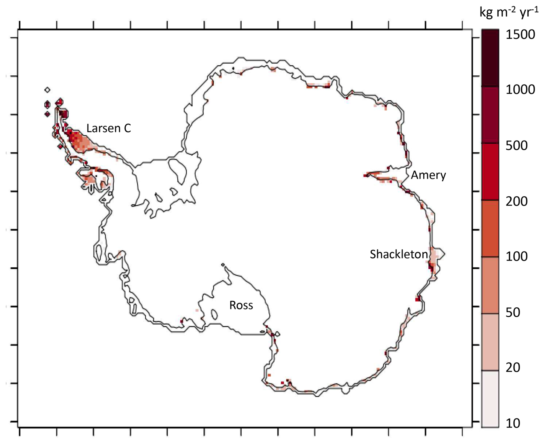
Figure A1 Average production of liquid water beyond firn saturation ($\mathrm{kg}{\mathrm{m}}^{-\mathrm{2}}{\mathrm{yr}}^{-\mathrm{1}}$) in MAR driven by the ERA5 reanalysis over 2015–2022.

Appendix B: Rationale for neglecting rainfall in the emulation

In the emulation method described in Sect. 2.3, we assume that precipitation is entirely made of snow and that the excess liquid water only originates from surface melting. This means that rainfall has been neglected, and this section provides further motivation for this assumption as well as an evaluation of the resulting error.

The only RCM simulation that we have until 2200 (MAR–IPSL-CM6A-LR, SSP5-8.5) indicates that precipitation mostly consists of snowfall all along the 21st century (Fig. B1). At 2100, the total precipitation includes 3 % of rainfall over the grounded ice and 12 % over the ice shelves. The proportion of rainfall increases along the 22nd century to reach 14 % over the grounded ice and 43 % over the ice shelves at 2200. Interestingly, from 1980 to 2200, rainfall always represents 10 % to 20 % of the surface melt rate for both the grounded ice and the ice shelves (Fig. B1).

To assess the impact of non-zero rainfall, we use Appendix B of Donat-Magnin et al. (2021) in which it is demonstrated that liquid water is produced beyond firn saturation if

$$\begin{array}{}\text{(B1)}& {\displaystyle \frac{\mathrm{MLT}+\mathrm{RF}}{\mathrm{SNF}-\mathrm{MLT}}}>{\displaystyle \frac{{\mathit{\rho }}_{\mathrm{co}}}{{\mathit{\rho }}_{\mathrm{s}}}}-\mathrm{1},\end{array}$$

where MLT is the surface melt rate, SNF the snowfall rate, RF the rainfall rate, ρ_co the firn close-off density (830 kg m⁻³ in the following), and ρ_s the fresh snow density (300 kg m⁻³ in the following). If RF=0, Eq. (B1) becomes Eq. (3) with $r=({\mathit{\rho }}_{\mathrm{co}}-{\mathit{\rho }}_{\mathrm{s}})/{\mathit{\rho }}_{\mathrm{co}}=\mathrm{0.64}$.

First, let us consider the impact of neglecting rainfall before melting as a source of liquid water in the firn. At most, rainfall reaches RF=0.20 MLT (Fig. B1), and in this case, Eq. (B1) can be rewritten as

$$\begin{array}{}\text{(B2)}& {\displaystyle \frac{\mathrm{MLT}}{\mathrm{SNF}}}>{\displaystyle \frac{{\mathit{\rho }}_{\mathrm{co}}-{\mathit{\rho }}_{\mathrm{s}}}{{\mathit{\rho }}_{\mathrm{co}}+\mathrm{0.2}{\mathit{\rho }}_{\mathrm{s}}}}.\end{array}$$

Hence, accounting for rainfall is equivalent to having an effective r threshold of 0.60 instead of 0.64, which has a relatively small effect (see sensitivity to r in Fig. 2).

Second, let us consider the consequence of having a precipitation that is partly liquid, assuming that the Clausius–Clapeyron relationship (Eq. 1) is valid for the total precipitation. For the ice shelves at year 2100, we can write RF=0.12 PR and SNF=0.88 PR (Fig. B1b), where PR is the total precipitation rate. In this case, Eq. B1 becomes

$$\begin{array}{}\text{(B3)}& {\displaystyle \frac{\mathrm{MLT}}{\mathrm{PR}}}>{\displaystyle \frac{\mathrm{0.88}{\mathit{\rho }}_{\mathrm{co}}-{\mathit{\rho }}_{\mathrm{s}}}{{\mathit{\rho }}_{\mathrm{co}}}}.\end{array}$$

Here, accounting for rainfall is equivalent to having an effective threshold r of 0.52 instead of 0.64, which has a relatively small effect (see sensitivity to r in Fig. 2). A similar calculation for the ice shelves at year 2200 (RF=0.43 PR) gives an effective threshold r of 0.21. This means that for a given melt rate, runoff is produced more easily than predicted by our emulation method due to the decreasing proportion of solid precipitation toward year 2200. The ice shelf surface melt rate at 2200 is nonetheless much higher than the snowfall rate (Fig. B1b), so the excess liquid water is only underestimated by 11 % if we use r=0.64 instead of r=0.21 (from the third line of Eq. 4).

We conclude that neglecting rainfall in our emulation is a good assumption until 2100 that remains reasonable until 2200, when melting prevails.

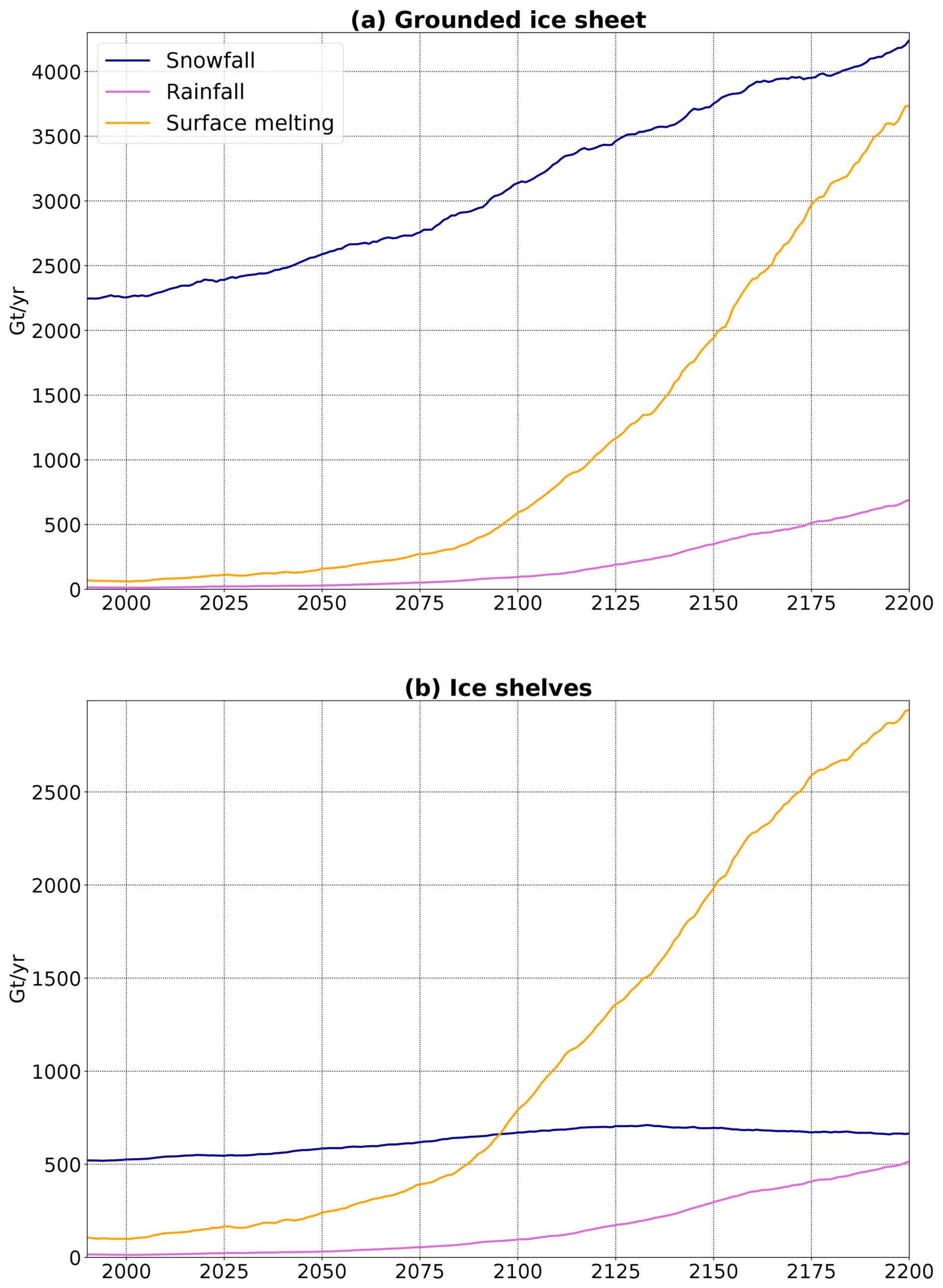
Figure B1 Total snowfall, rainfall, and surface melting at the surface of (a) the grounded ice sheet and (b) the ice shelves in the MAR–IPSL-CM6A-LR–SSP5-8.5 simulation. A running average of 21 years has been used for all time series.

Appendix C: Exponential fits in the parameter calibration

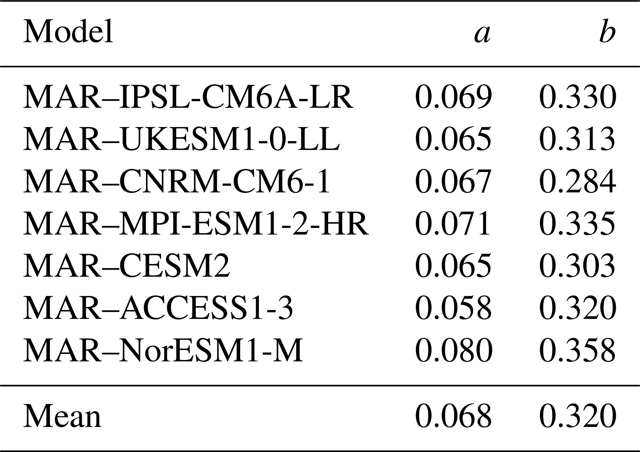
The a and b parameters of Eq. (4) are obtained through a least-mean-squares fitting of an exponential curve for SMB minus runoff on the one hand and the surface melt rate on the other hand (Fig. C1). The fitted dataset includes the 1980–2100 period, and the 20-year reference period is 2041–2060. To remove outliers, we only consider points between the 5th and the 95th percentile of the SMB minus runoff distribution and the points where the melt rate is greater than its 75th percentile. The calibrated a and b parameters are listed in Table C1 for individual models.

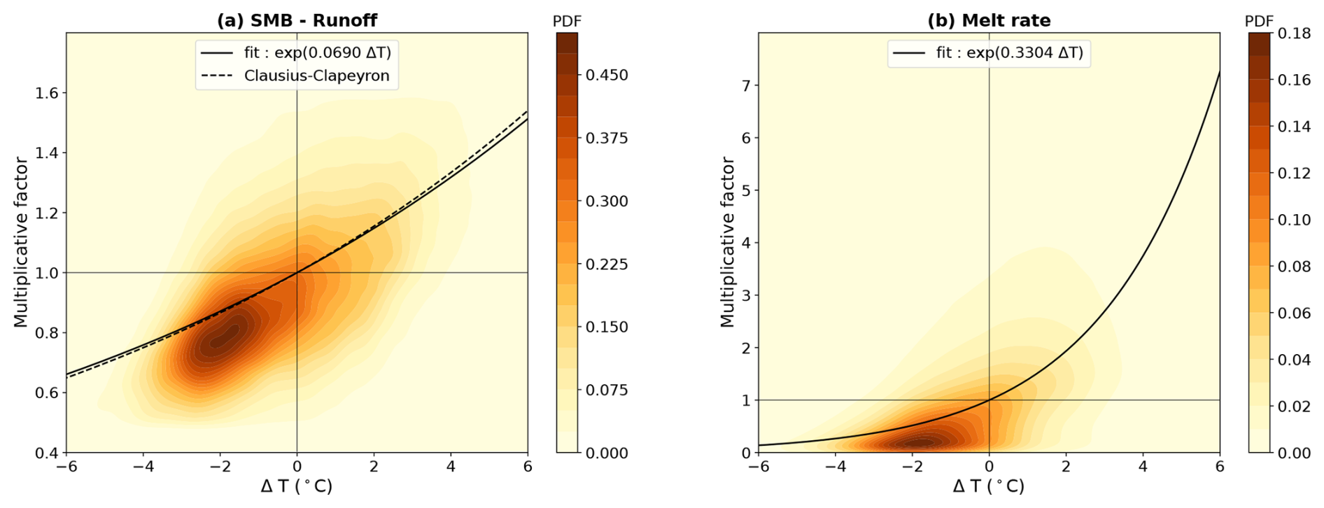
Figure C1 Factor by which the SMB minus runoff (a) and the surface melt rate (b) are multiplied versus the associated ΔT with respect to 2041–2060. This plot corresponds to MAR–IPSL-CM6A-LR. The probability density function (PDF) is calculated through a Gaussian kernel density estimate from the annual means at every grid point on the ice sheet. The dashed line in panel (a) represents the Clausius–Clapeyron exponential law.

Table C1 Fit parameters for accumulation and melt rate (see Eq. 4).

Appendix D: Evaluation of the emulated SMB spatial patterns

Here we provide evidence that the three applications of our emulation method (Fig. 1) are able to represent the spatial SMB patterns (Figs. D1, D2, D3). For a reason that remains elusive, the largest mismatch is found on the Ross Ice Shelf, where the emulation produces a negative SMB around 2100 for the three applications, while it remains mostly positive in the original MAR simulation.

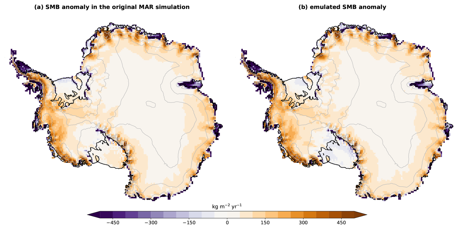
Figure D1 Evaluation of the emulation from another period (Fig. 1a). Mean SMB anomaly over 2101–2120 under the SSP5-8.5 scenario (a) simulated by MAR–IPSL-CM6A-LR and (b) emulated for the 2081–2100 period. The anomalies are calculated with respect to the 1995–2014 mean.

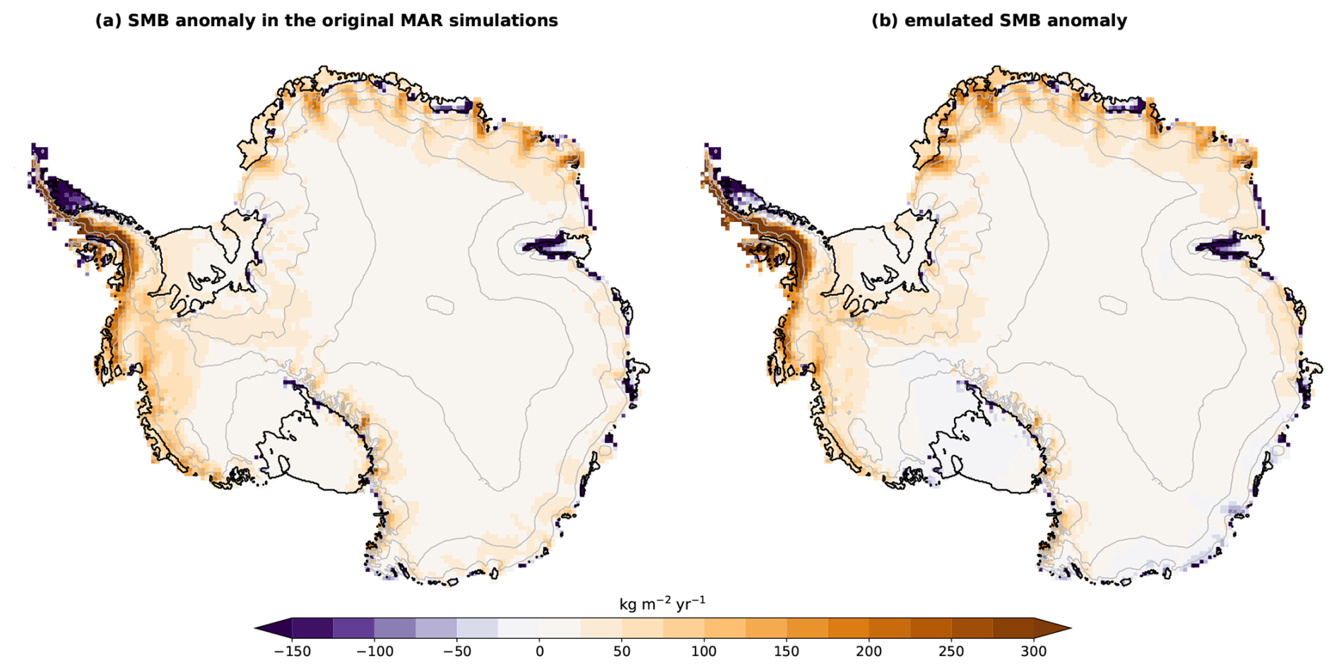
Figure D2 Evaluation of the emulation from another scenario (Fig. 1b). Mean SMB anomaly over 2081–2100 under the SSP2-4.5 scenario (a) simulated by three MAR simulations (MAR–CESM2, MAR–UKESM1-0-LL, and MAR–MPI-ESM1-2-HR) and (b) emulated for the corresponding MAR simulations under the SSP5-8.5 scenario. The anomalies are calculated with respect to the 1995–2014 mean.

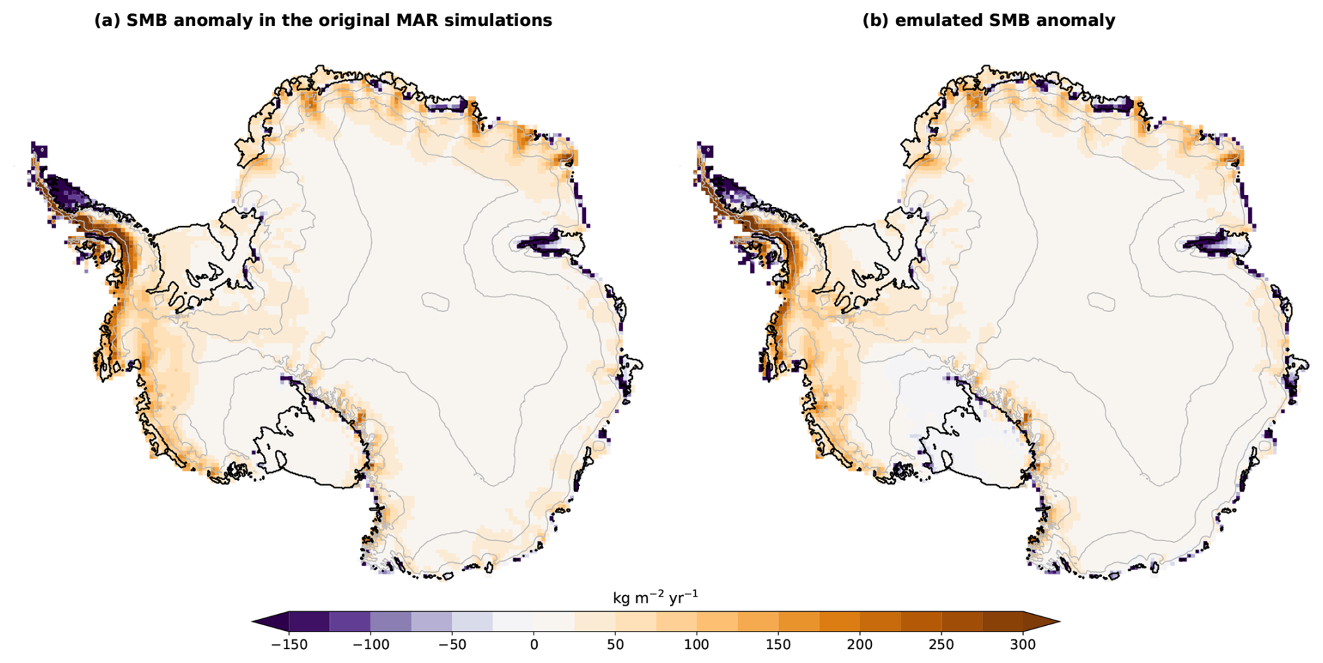
Figure D3 Evaluation of the emulation from MAR simulations driven by five other CMIP models (Fig. 1c). Mean SMB anomaly over 2081–2100 under the SSP2-4.5 scenario (a) simulated by three MAR simulations (MAR–CESM2, MAR–UKESM1-0-LL, and MAR–MPI-ESM1-2-HR) and (b) emulated for these three models from MAR simulations driven by five other CMIP models (as in Fig. 5). The anomalies are calculated with respect to the 1995–2014 mean.

Appendix E: Ice shelf surface mass balance

Here we describe the surface mass balance of ice shelves, which is relevant for the estimation of the ice shelf thinning rate, which can mechanically precondition hydrofracturing. In this appendix, and only here, we assume that the excess liquid water over the ice shelves is entirely removed as runoff, i.e. that there is no ponding. This is somewhat inconsistent with our assumptions in Sect. 3.2 and gives SMB estimates that are slightly underestimated in warm conditions.

Our projections indicate that the SMB over ice shelves has slightly increased over the 19th and 20th centuries, and it is not expected to significantly evolve throughout the 21st century under SSP1-2.6 and SSP2-4.5 (Fig. E1). The SMB even increases by a few tens of Gt yr⁻¹ along the 22nd century under SSP1-2.6 (Fig. E2).

The SSP5-8.5 SMB projections over ice shelves have a considerable spread, with a median close to present-day values and most of the weighted distribution within the historical range until 2100, but the 5th percentile approaches −400 Gt yr⁻¹ of anomaly by 2100 (Fig. E1). This is due to the emerging importance of ice shelf runoff at the end of the 21st century in the warmest simulations.

The ice shelves under SSP5-8.5 experience a net surface mass loss after 2090 to 2125 (depending on the model), with the exception of MAR–GISS-E2-1-H that stabilizes slightly above the zero SMB limit. The most extreme surface mass loss at 2200 is reached by MAR–CanESM5, which has the highest ECS of our ensemble and is equivalent to an average ice shelf thinning rate of 2 m yr⁻¹ (assuming an ice density of 920 kg m⁻³). Spatially, runoff anomalies overwhelm accumulation anomalies for several ice shelves of the Antarctic Peninsula before 2100 in the three scenarios (Fig. 10), and this becomes more widespread around Antarctica after 2100 under SSP5-8.5 (Fig. 11). In East Antarctica, runoff anomalies first prevail near the ice shelf grounding lines (Fig. 10), likely due to the diabatic heating of downsloping katabatic winds and enhanced melt–albedo feedback, as previously observed by Lenaerts et al. (2017).

Figure E1 Emulated ensemble of surface mass balance over the Antarctic ice shelves for the historical period and three SSP scenarios. The median and percentiles are calculated based on the 16-model ensemble weighted to match with the very likely range of ECS (see Sect. 2.4). A 21-year running average has been used for all the time series.

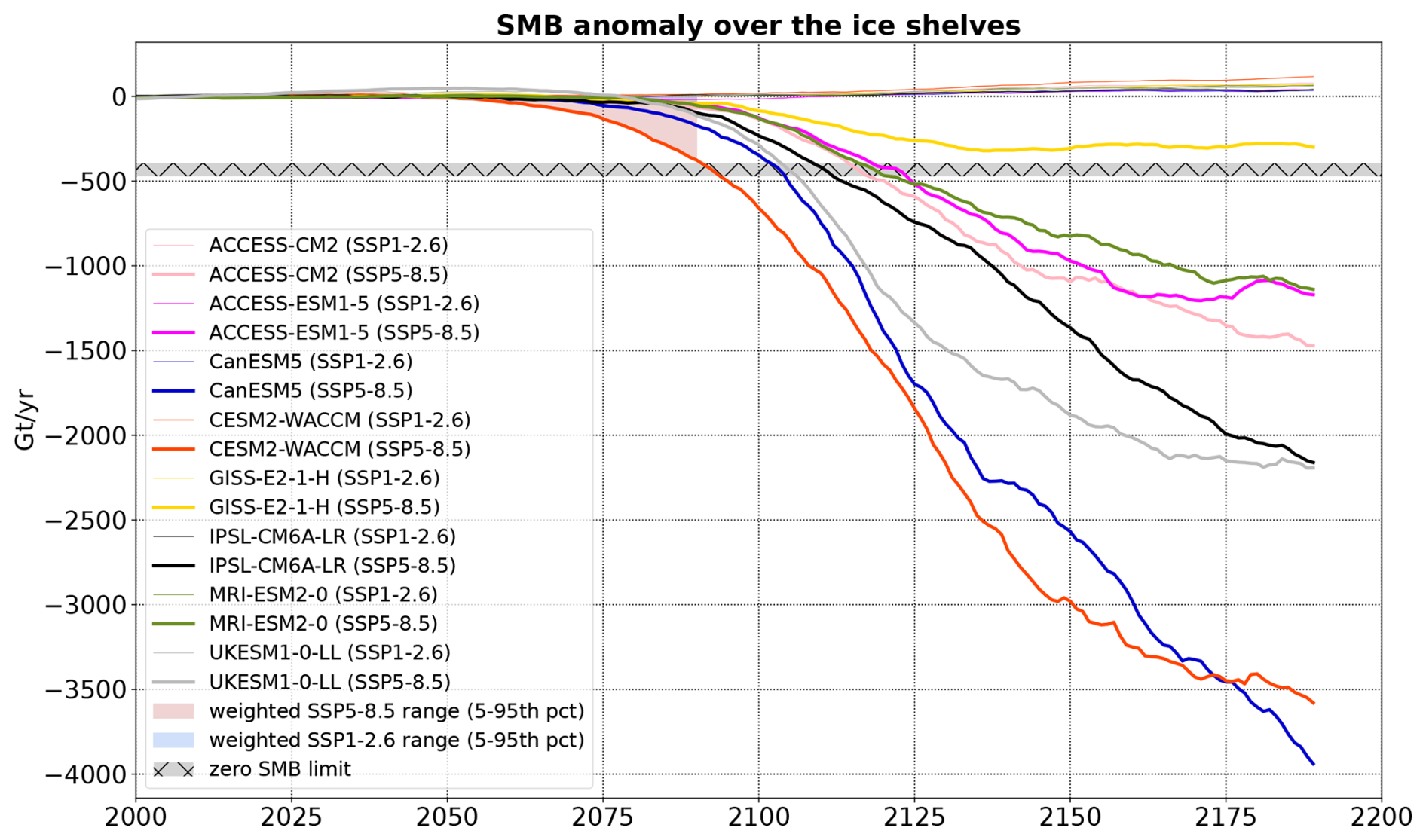
Figure E2 Eight emulations of surface mass balance over the Antarctic ice shelves for the SSP-1.26 and SSP5-8.5 scenarios. The very likely range from 16 emulations over 2000–2100 (same as Fig. E1) is also shown. The hatched area indicates the anomaly interval at which SMB reaches zero according to the MAR, RACMO, and HIRHAM present-day values reported in Mottram et al. (2021). A 21-year running average has been used for all the time series.