the Creative Commons Attribution 4.0 License.
the Creative Commons Attribution 4.0 License.
A hybrid ice-mélange model based on particle and continuum methods
Saskia Kahl
Carolin Mehlmann
Dirk Notz
Ice mélange, a composite of sea ice and icebergs, can have a major influence on sea-ice–ocean interactions. However, ice mélange has not been represented in climate models because numerically efficient realizations do not exist. This motivates the development of a prototype of a dynamic hybrid ice-mélange model that we present in this paper. In our approach, icebergs are included as particles, while sea ice is treated as a continuum. To derive a joint continuum for ice mélange, we integrate particle properties into the sea-ice continuum. Thus, icebergs are viewed as thick, compact pieces of sea ice. The ice-mélange formulation is based on the viscous–plastic sea-ice rheology, which is currently the most widely used material law for sea ice in climate models. Starting from the continuum mechanical formulation, we modify the rheology such that icebergs are held together by a modified tensile strength in the material law. Due to the particle approach, we do not need highly resolved spatial meshes to represent the typical size of icebergs in ice mélange (< 300 m). Instead, icebergs can be tracked on a subgrid level, while the typical resolution of the sea-ice model can be maintained (≥10 km). This is an appealing property for computational efficiency and for an inclusion within large-scale models. In idealized test cases, we demonstrate that the proposed changes in the material law allow for a realistic representation of icebergs within the viscous–plastic sea-ice rheology. Furthermore, we show that subgrid dynamics, such as polynya formation due to grounded icebergs, can be modelled with the hybrid approach. Overall, this suggested extension of the viscous–plastic sea-ice model is a promising path towards the integration of ice mélange into climate models.
- Article
(2892 KB) - Full-text XML
- BibTeX
- EndNote
Fjords with marine-terminating glaciers are commonly found in the polar regions, e.g. around Greenland. These fjord systems can be filled with sea ice into which icebergs calve so that a mixture of sea ice, bergy bits and icebergs is formed: ice mélange. The ice mélange consists of many interacting small icebergs (<300 m) (Dowdeswell et al., 1992; Sulak et al., 2017).
Observations based on field campaigns and remote sensing data indicate that ice mélange affects the glacier–fjord system either by releasing fresh water into the fjord (Enderlin et al., 2018; Moon et al., 2018; Mortensen et al., 2020) or by creating a force at the glacier termini (Cassotto et al., 2015; Bevan et al., 2019; Xie et al., 2019). This force might have enough strength such that it prevents calving events (e.g. Amundson et al., 2010; Krug et al., 2015; Bassis et al., 2021), whereas the release of fresh water through icebergs influences the fjord circulation and melting at the glacier termini (Davison et al., 2020).
Observing ice mélange is difficult, due to the sparsity of remote sensing data and due to the challenges of taking in situ measurements in dense ice conditions. To obtain insights into the potential impact of ice mélange on glacier calving and the underlying ocean circulation, numerical models are therefore necessary. The existing approaches used to include ice mélange into models vary in their complexity. They range from the full description of the ice-mélange dynamics (Robel, 2017; Burton et al., 2018) to the parameterization of specific interactions such as the load which the ice mélange creates at the glacier termini (Schlemm and Levermann, 2021).
There are two distinct approaches in the scientific literature to model the dynamics of ice mélange. In particle methods the ice mélange is expressed using discrete interacting particles, with single particles representing icebergs or sea-ice floes (e.g. Robel, 2017; Burton et al., 2018). As discussed by Vaňková and Holland (2017), implementing a full particle approach into climate models would be extremely challenging due to the enormous numerical costs. In contrast, in the continuum approach, the ice mélange is prescribed as a single continuum (e.g. Pollard et al., 2018; Amundson et al., 2024).
To provide a simple coupling between ice-mélange and sea-ice modules used in climate models, Vaňková and Holland (2017) introduced a continuum ice-mélange model, where sea ice and icebergs build a joint continuum. Icebergs are represented via thick compact pieces of sea ice, which are tracked with a Lagrangian advection using moving meshes. In their model, the icebergs are held together via a large tensile (and shear) strength, which is introduced by a modification of the underlying cavitating fluid sea-ice rheology (Flato and Hibler, 1992). The approach of Vaňková and Holland (2017) requires a high spatial resolution to resolve icebergs in the ice mélange. It is challenging to efficiently solve the nonlinear momentum equation of the underlying sea-ice model with existing solvers (Koldunov et al., 2019; Mehlmann and Richter, 2017b). Currently, efficient solvers for the ice-mélange model of Vaňková and Holland (2017) are missing.
To overcome these difficulties, we introduce a hybrid ice-mélange model. In this approach, the ice mélange is described as a joint continuum consisting of sea ice (continuum) and icebergs (particles). The use of particles in the hybrid approach allows us to track the icebergs on a subgrid level. This has the advantage that icebergs do not need to be explicitly resolved by the spatial mesh. Thus, the typical grid size of several kilometres for a sea-ice model can be used to simulate ice mélange. We derive the momentum equation of the ice mélange by selectively modifying the tensile strength of the sea-ice rheology. This concept is similar to the approach of Vaňková and Holland (2017), but instead of applying the cavitating fluid sea-ice rheology, we consider the viscous–plastic (Hibler, 1979) material law, which has been shown to be more realistic than the cavitating fluid model (Kreyscher et al., 2000).
So far, most climate models have treated sea ice as a viscous–plastic material using the viscous–plastic (Hibler, 1979) or elastic–viscous–plastic (Hunke and Dukowicz, 1997) sea-ice rheology. These rheologies are used in 30 out of the 33 global climate models of the Climate Model Intercomparison Project 5 (CMIP5) (Stroeve et al., 2014). Furthermore, the study of Amundson and Burton (2018) indicates that ice mélange exhibits viscous–plastic deformations. Thus, an inclusion of ice mélange into climate models via a modification of the viscous–plastic material law is a promising approach.
The paper is structured as follows. Sect. 2 presents the ice-mélange model, and Sect. 3 outlines the used numerical discretization. The model is numerically evaluated in Sect. 4. We discuss our results in Sect. 5 and summarize our conclusions in Sect. 6.
Based on the representation of the sea-ice dynamics with a viscous–plastic rheology, we develop a model for ice mélange. As in the underlying sea-ice model (Hibler, 1979), the ice-mélange model consists of three prognostic variables: the ice-mélange's thickness H, its concentration A within a specific grid cell and horizontal velocity v. Ice mélange is considered a joint continuum of sea ice and an iceberg distribution, integrated from a set of iceberg particles {p}. On the continuum level, the icebergs are interpreted as thick and compact pieces of sea ice. Every iceberg is represented by a disc-shaped particle p, which is described by a radius rp and a height hp, which can vary between the icebergs. We assume that icebergs are represented by a finite number of small, disc-shaped particles. Thus, the continuum thickness and concentration of ice mélange are described as
Here, Ω is the two-dimensional domain of interest, x and y are the horizontal spatial coordinates, and t is the time. In order to model the ice-mélange velocity, we formulate an expansion of the viscous–plastic rheology that accounts for icebergs. To keep icebergs (thick and concentrated pieces of ice) in the ice-mélange formulation together, we modify the tensile strength of the viscous–plastic law.
In the following, we first generally review the formulation of the governing equations (Sect. 2.1) and the viscous–plastic rheology (Sect. 2.2) before we modify its strength parameterization (Sect. 2.3) to represent icebergs. The iceberg particle interaction and the coupling to the continuum ice-mélange formulation are outlined in Sect. 2.4.
2.1 Momentum and conservation equation
The drift of the ice mélange is described by the two-dimensional momentum equation:
where ρ=900 kg m−3 is the ice density, and ∇⋅σ describes the divergence of the two-dimensional symmetric stress tensor. The internal stresses are given by the material law described in Sect. 2.3. The remaining terms collected in Fb,
model the body forces acting on the ice mélange: the Coriolis parameter f with upward-pointing unit vector k, the gravity constant g, the surface height Hd, and the atmospheric and oceanic stresses given by τatm and τocean. These two drag terms (Coon, 1980) are expressed as
where vatm describes the wind velocity and vocean the ocean current. The corresponding densities are given by ρatm=1.3 kg m−3 and ρocean=1026 kg m−3. The drag coefficients are and . Note that ∥⋅∥2 represents the Euclidean norm. The advection of the sea-ice thickness Hsea ice and the concentration Asea ice are calculated as
with and . The icebergs are advected based on the continuum ice-mélange velocity v:
where is the position of the centre of particle p.
2.2 Viscous–plastic rheology
Let be the principal components of the stress tensor σ, given by
In the viscous–plastic model (Hibler, 1979), the states of the stress, σ, are described by an elliptic yield curve of the form
where e=2 is the minor axis of the ellipse, and P is the ice strength modelled as
with strength parameter N m−2, and C=20. The yield curve is expressed in terms of the principal components of the stress tensor σ:
A visualization of the yield curve is given in Fig. 1 (blue line). As there are no stress states on the yield curve with , sea ice has no tensile strength (no resistance to divergence) (Leppäranta, 2011). The stress states are related to the strain rates,
by the constitutive law (Hibler, 1979):
where δij is the Kronecker symbol. The nonlinear shear ζ and bulk viscosity η are chosen as
To guarantee a smooth transition between the viscous and the plastic regime, we follow Kreyscher et al. (2000) and choose
In the case of the plastic regime, is defined as
The viscous regime is given as
2.3 Strength parameterization
The absence of tensile strength in the original model is apparent from the fact that the yield curve of the viscous–plastic rheology does not contain combinations of (see the blue curve in Fig. 1). A tensile strength has been introduced into this model, e.g. by König and Holland (2010) to model landfast sea ice. Similar to Vaňková and Holland (2017), which added a tensile strength into a cavitating fluid model in order to prescribe ice mélange, we introduce a tensile strength into the standard viscous–plastic sea-ice rheology to model icebergs. This tensile strength leads to a resistance to divergence in the presence of icebergs.
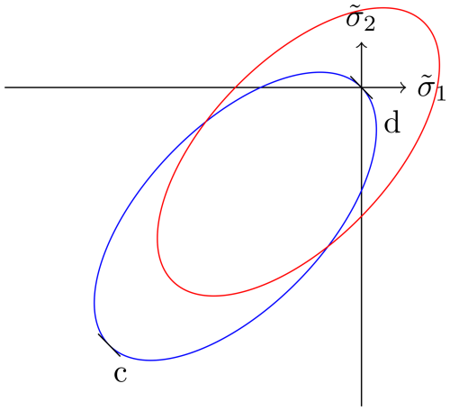
Figure 1Two-dimensional yield curve in principal stress space without (blue) and with (red) tensile strength. Pure divergence d is at the origin of the graph; pure convergence is obtained at c. and are the principal components of the stress tensor σ (see Eq. 14).
By including the tensile strength, the elliptic yield curve is shifted into the first quadrant (red curve in Fig. 1). The new centre of the ellipse is given by , with the maximum tensile strength T. Both P and T are positive numbers. Thus, the modified elliptic yield curve is given by
with the elliptic ratio e. For T=0 (no tensile strength), the elliptic yield curve is equivalent to the ellipse of the viscous–plastic sea-ice rheology (see Eq. 10). It is assumed that ∂F and the strain rates are perpendicular to the surface of the yield curve (Leppäranta, 2011). Thus, the relation between the stress tensor and the strain rates for the shifted yield curve is derived by a normal flow rule:
with γ>0. This leads to the modified rheology
with the bulk and shear viscosities as
Following König and Holland (2010), we define the tensile strength T relative to the compressive strength:
The indicator function Φ is given as
2.4 Iceberg interaction
An interaction of two distinct particles pi and pj is modelled by a hard disc model (Herman, 2011) if the particles overlap:
where ri and rj are the radii, and and are the positions of the interacting particles pi and pj, respectively. The position of the overlapping particles is corrected by assuming an inelastic collision (Herman, 2011). For this, we use the last particle position at which the particles had not collided and update the location of the particles based on the ice-mélange velocity corrected for the collision. The latter is calculated as follows:
where and are the current velocities of the ice mélange, and mi and mj are the masses of particle pi and pj, respectively. The coefficient αij is given by
with the relative unit position . The coefficient of restitution ϵ is set to 0.9, as this value has been used in the past for sea ice (Shen et al., 1987). Since we assume that icebergs are thick pieces of sea ice, this choice is appropriate.
The ice-mélange model is implemented in the open-source academic software library Gascoigne (Braack et al., 2021), which uses quadrilateral grids. On the mesh, the velocity unknowns are placed at the vertices, whereas the tracers are staggered at the cell centres. This placement corresponds to an A-grid- and a B-grid-type staggering for the velocity and tracers, respectively. The velocity is approximated in space with piecewise linear finite elements, whereas the tracers are discretized as a piecewise constant per cell.
For the time discretization of the ice-mélange model, we split the coupled system of equations in time. First, we approximate the solution of the momentum equation (Eq. 3). Then, the solution of the transport (Eqs. 7 and 8) with the updated velocity is computed. This choice of the implicit Euler method is motivated by the fact that an explicit discretization of the viscous–plastic sea-ice model requires a time step of 1 s on a grid with a size of 100 km × 100 km (Ip et al., 1991). We expect similar constraints for the ice-mélange model, because its rheology is based on the viscous–plastic sea-ice model.
For our choice of an implicit temporal discretization, a nonlinear system of differential equations needs to be solved in every time step. We use a modified Newton method for this solution as it shows improved convergence compared to a standard Newton method and Picard solver (Mehlmann and Richter, 2017a).
3.1 Coupling between particle and continuum method
In order to derive the continuum thickness and concentration of the ice mélange, the icebergs in the form of particles need to be numerically coupled into the continuum sea-ice formulation. We realize this by calculating a continuum iceberg thickness and iceberg concentration in each cell K:
with particle area and area of a grid cell . We use the iceberg concentration to determine the tensile strength in the presence of icebergs. Thus, the discretized version of the tensile strength is given by
In the discretized version, we account for the sea-ice concentration weighted by a constant ctensile. For the sake of simplicity, we choose ctensile=1. The inclusion of the sea-ice concentration allows us, for example, to model no tensile strength between icebergs if there is no sea ice present.
The threshold is selected such that the tensile strength becomes active as soon as an area of the grid cell is filled with icebergs that cover an area at least as large as a disc-shaped iceberg with radius of . This choice is discussed in Sect. 5.
The ice-mélange concentration and thickness in each grid cell are given by
In the presence of icebergs, sea ice is more compressed and thicker compared to areas without icebergs. The effective sea-ice thickness and sea-ice concentration are given by and , respectively. In the context of this ice-mélange formulation, we assume that icebergs are represented by a finite number of small particles with .
We summarize the time discretization of the ice-mélange dynamics in Algorithm 1. The time loop starts with the calculation of the iceberg distribution (Eq. 28) and the computation of the ice-mélange tracers (Eqs. 31, 32), which corresponds to step 1 and step 2 of Algorithm 1. Then, the updated ice-mélange tracers are coupled to the momentum equation to solve for the ice-mélange velocity (step 3 of Algorithm 1). To calculate the advection of ice mélange in Eqs. (7) and (8), we separately transport the continuum sea-ice tracers and the iceberg particles (step 4 and step 5 of Algorithm 1, respectively). Sea ice in Eq. (7) is advected via an upwind scheme, while the particles are transported according to Eq. (8) in a substepping procedure. With this approach, each particle is advected with the corresponding ice-mélange velocity. The latter is given by evaluating the piecewise linear finite element interpolation at the particle location. During the substepping procedure, the icebergs are checked for collisions with other icebergs or with the boundary of the domain and then replaced accordingly to Eq. (26).
Algorithm 1Partitioned time-stepping loop.
-
Derive an average iceberg concentration Aiceberg(tn) and iceberg thickness Hiceberg(tn) (Eq. 28) based on the set of corresponding particle positions {xp(tn−1)}.
-
Calculate the ice-mélange concentration A(tn) (Eq. 31) and ice-mélange thickness H(tn) (Eq. 32) based on the concentration and thickness of the continuum sea-ice and iceberg distribution, and Hiceberg(tn−1), respectively.
-
Solve the momentum equation (Eq. 3) based on A(tn) and H(tn):
-
Solve the advection Eq. (7) based on the velocity v(tn):
-
Based on a partitioning into equidistant substeps , calculate for the particle position (Eq. 8) based on v(tn) and account for particle interaction in the case of collision between particles (Eq. 26):
The proposed hybrid ice-mélange model is tested in six idealized test cases. The first three test cases (Sect. 4.1) highlight the need for introducing a tensile strength for icebergs into the viscous–plastic sea-ice rheology. Based on the verification of the modified tensile strength, we numerically analyse the combination of particle and continuum methods to represent ice mélange in the last three test cases (Sect. 4.2).
4.1 Tensile strength
The first three test cases are designed such that the behaviour of the ice mélange is tested under compressive (Sect. 4.1.1), tensile (Sect. 4.1.2) and shear (Sect. 4.1.3) forces. For the sake of simplicity, we use vocean=0 m s−1. In order to reduce the complexity of the analysis of the modified tensile strength, we neglect the particle coupling in these first three test cases. Instead of simulating the iceberg motion via particles and integrating it into the sea-ice continuum, we track the icebergs (thick and compact pieces of sea ice) in the sea ice via an indicator function ϕ that is transported in time:
where δxy is the Kronecker symbol that equals 1 in the presence of icebergs. According to the volume-in-fluid method (Hirt and Nichols, 1982), the indicator function Φ of Eq. (23) is modified to
We have chosen c=0.3 by experimental tuning.
4.1.1 Iceberg pushed against a wall
The first test case is similar to the one used by Vaňková and Holland (2017). The domain is given by an area of the size 5 km × 5 km; see left plot in Fig. 2. All boundaries except the exit to the ocean (right boundary) use Dirichlet boundary conditions (v=0). The upper and lower boundaries represent coastlines, while the boundary on the left represents the glacier terminus. We place a 1 km × 2 km large iceberg in front of the glacier wall. A grid cell size of 110 m is used. The iceberg is a 10 m thick compact block of sea ice with a concentration of 1. The left half (<2.5 km) of the domain is filled with 0.1 m thick sea ice with a concentration of 0.1. The iceberg is pushed against the glacier terminus by a constant wind vatm=20 m s−1.
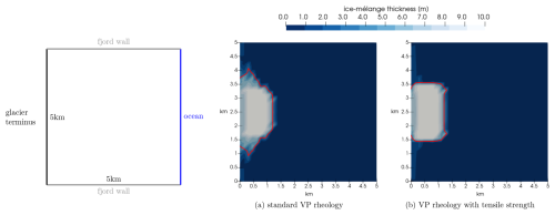
Figure 2Visualization of the ice-mélange thickness for a test case in which an iceberg (thick red contour line) is pushed against the glacier terminus (left boundary) by a constant wind (vatm=20 m s−1). The panels denote the results for (a) the standard viscous–plastic (VP) rheology and (b) for the viscous–plastic rheology with tensile strength. Both snapshots show the simulation result after 3 h.
The simulation is run for 3 h. When comparing the standard viscous–plastic rheology and the modified material law (Fig. 2), we find that for the standard viscous–plastic rheology the thick and compact piece of sea ice, which models the iceberg, deforms towards the glacier and accumulates in front of the glacier terminus. This is visible by the thick red line shown in Fig. 2a, which visualizes the iceberg's contour. The sea ice along the glacier terminus (outside the contour line) piles up. With the proposed modification, the iceberg is able to keep its rectangular shape throughout the simulation (see Fig. 2b). This test case shows that in our modified viscous–plastic rheology, the iceberg can withstand the compression, initiated by the wind forcing.
4.1.2 Iceberg under a divergent wind field
We consider a 5 km × 5 km large domain with a divergent wind field:
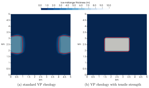
The 10 m thick iceberg with a concentration of 1 is placed in the middle of the domain. The whole domain is filled with sea ice whose concentration is 0.1 and whose thickness is 0.1 m. Using the standard viscous–plastic rheology, the iceberg is torn apart after 3 h (see Fig. 3a). With additional tensile strength, the iceberg keeps its form (see Fig. 3b). The surrounding sea ice is still transported in the wind direction. This test case shows, in particular, that the iceberg maintains its shape under diverging wind conditions at the location of the iceberg.
4.1.3 Iceberg under shear
In the third test case, the same initial setup as in Sect. 4.1.2 is used. But instead of using a divergent wind field, we apply a shearing wind field:
The domain of size 5 km × 5 km is filled with 0.1 m thick sea ice with a concentration of 0.1.
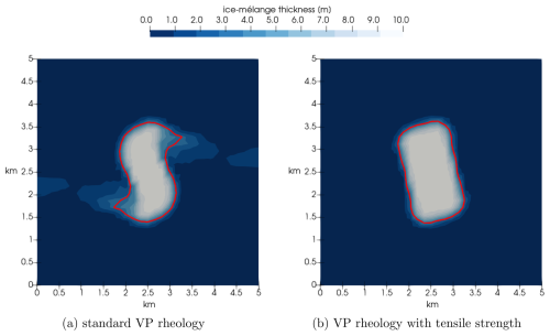
Figure 4The iceberg is placed under a shearing wind field ( m s−1). Panel (a) visualizes the result for the standard viscous–plastic (VP) rheology and (b) for the viscous–plastic rheology with tensile strength. Both snapshots show the ice-mélange thickness after 3 h. The thick red line indicates the iceberg contour.
In both cases, the iceberg rotates clockwise (see Fig. 4) as expected. Using the standard viscous–plastic rheology, the iceberg deforms. Fig. 4a shows that the iceberg contour is slightly S-shaped, and parts from the iceberg already detach. This is in contrast to the behaviour of the iceberg using the additional tensile strength (see Fig. 4b). Here, the iceberg contour stays rectangular, and the iceberg rotates as one sea-ice block.
4.2 A hybrid ice-mélange representation
The advantage of using a particle method on the joint continuum of sea ice and icebergs is given by the fact that the icebergs and their interactions can be modelled on a subgrid-scale. We consider a domain of size 512 km × 512 km covered with a quadrilateral mesh of size 16 km. In this setup, icebergs are represented by particles with a radius of 125 m. Using this configuration, we study an iceberg–iceberg interaction under shear forcing (Sect. 4.2.1), iceberg separation under divergent forcing (Sect. 4.2.2) and the formation of a polynya due to subgrid iceberg grounding (Sect. 4.2.3). All test cases use a time step size of 2000 s.
4.2.1 Iceberg–iceberg interaction
An explicit iceberg–iceberg collision is forced in order to test the behaviour of icebergs under contact. Two icebergs with a height of 20 m are placed into a 2 m thick sea-ice field with a concentration of 0.7. The icebergs approach each other due to the following wind field:
The velocity field of the ice mélange after the first time step is shown in Fig. 5a. At first, the icebergs approach each other until they collide (Fig. 5b). Due to collision, iceberg 1 moves further up and iceberg 2 further down. After the collision event, both icebergs drift past each other and separate again; see Fig. 5c.
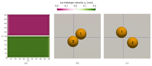
Figure 5Visualization of the first component, vx, of the ice-mélange velocity for a test case in which two icebergs are transported towards each other by a constant wind ( m s−1). Panel (a) shows the whole domain with the initial velocity field. The last two panels show a closeup of the iceberg interaction after (b) 100 time steps and after (c) 200 time steps with a time step size of 2000 s.
4.2.2 Iceberg field under diverging winds
We analyse the response of an iceberg field to diverging winds and consider the following wind field:
The icebergs used in the setup are 20 m thick. The sea ice, if present, has a concentration of 0.7 and a thickness of 2 m. To highlight the influence of the tensile strength (Eq. 30) on the motion of the iceberg field, we compare different setups in Fig. 6.
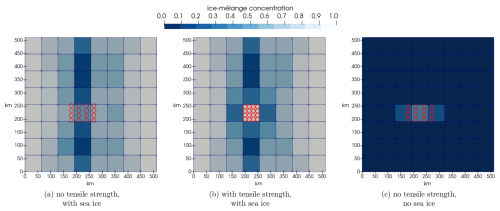
Figure 6Iceberg field under a diverging wind field. The icebergs have a height of 20 m. In panels (a) and (b), sea ice is 2 m thick with a concentration of 0.7, while in panel (c) the icebergs have no surrounding sea ice. All three panels show the simulation after 300 time steps.
In Fig. 6a and b, sea ice is presented between and around the iceberg field. In contrast to Fig. 6b, the tensile strength parameterization is not active in Fig. 6a. Thus, the surrounding sea ice and the icebergs disperse in Fig. 6a. We use the same setup in Fig. 6b but with activated tensile strength. The surrounding sea ice moves apart, according to the wind field, but the iceberg particles stay in their initial grid cell. Without sea ice between and around the icebergs, the tensile strength in Eq. (30) equals zero. Therefore, the icebergs disperse in Fig. 6c. The setup shows that the modified rheology allows for icebergs to disperse if no sea ice is present. At the same time, we see that the tensile strength is necessary to prevent the field from moving in the case of an iceberg field with sea ice in between. The amount of active tensile strength can be controlled by the parameter ctensile (Eq. 30), and this is further discussed in Sect. 5.
4.2.3 Iceberg grounding
Icebergs can impact sea ice in different ways, e.g. mechanically by colliding and breaking up the sea-ice cover, by creating openings, and by altering the structure of the sea-ice cover. To simulate such an interaction, we simulate iceberg grounding in the final test case. Those grounding events occur in shallow waters and have profound implications for sea-ice dynamics. As icebergs come into contact with the seafloor, they become immobilized, transforming into obstacles that influence the surrounding sea ice. This affects the natural flow and movement of sea ice and thereby the local circulation patterns and the distribution of sea ice. In this test case, we simulate iceberg grounding and analyse the resulting dynamics of the ice mélange with respect to the formation of a polynya. The domain consists of a 2 m thick sea-ice layer with a concentration of 0.7. Three grid cells, each of the size of 16 km × 16 km, are filled with 4096 icebergs per cell (see Fig. 7). Each iceberg has a radius of 125 m and is 20 m thick. We use such a large number of icebergs to show that we can work with many icebergs per cell that are much smaller than the cell size. These icebergs represent the effects of multiple grounded icebergs in the area with different sizes.
The icebergs in the two lower grid cells closer to the boundary are marked as grounded (viceberg=0 m s−1). As forcing, we use an ocean current of vocean=0.2 m s−1 and neglect any atmospheric forcing (vatm=0 m s−1).
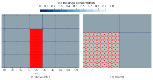
Figure 7Panel (a) shows the initial ice-mélange concentration of the grounded iceberg setup (the two lower grid cells). Panel (b) presents a closeup of the upper grid cell so that individual iceberg particles are visible.
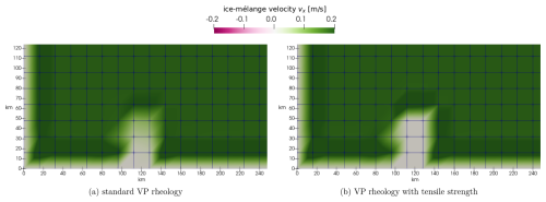
Figure 8Closeup of the ice-mélange velocity after five time steps of the grounded iceberg setup. The area of low velocity in the centre of the domain indicates the presence of the icebergs. The ice mélange is forced by a constant ocean current (vocean=0.2 m s−1).
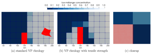
Figure 9Three grid cells are each filled with 4096 icebergs. The lower two grid cells consist of only grounded icebergs. The snapshots in (a) and (b) show the ice-mélange concentration after 600 time steps with an ocean forcing of vocean=0.2 m s−1. Panel (c) shows a closeup of the ungrounded icebergs in (b).
Figure 9a shows the grounding event using the standard viscous–plastic rheology. The ungrounded icebergs in the upper of the three cells are transported as one block of icebergs towards the right boundary. The square shape is slightly deformed and rotated. The surrounding sea ice accumulates in the domain's right half and builds a straight ice edge. This is a nonphysical behaviour as grounded icebergs should cause a pile-up of sea ice in front of the icebergs. Due to the missing tensile strength in this configuration, the ice-mélange velocity is not zero in the dense iceberg field; see Fig. 8a. Thus, the sea ice flows through the icebergs.
This is in contrast to the results conducted with the modified rheology (see Fig. 9b). Here, the additional tensile strength leads to nearly zero velocity in the dense iceberg field (Fig. 8b) and prevents the sea ice from passing through the icebergs. Therefore, sea ice accumulates in front of the icebergs. Compared to the setup with the standard viscous–plastic rheology, the icebergs move only slightly to the right in the configuration with the modified tensile strength. This is visible in the closeup shown in Fig. 9c. The active tensile strength in the upper of the three cells leads to a reduction in the ice-mélange velocity, which results in a smaller displacement of the iceberg particles.
The results from Sect. 4 show that the combined approach of subgrid iceberg particle dynamics and a continuum formulation is able to simulate ice-mélange dynamics with respect to different wind and ocean forcings. The usage of particle icebergs in the setup allows for a representation of ice mélange on coarse-resolution horizontal meshes, which have the same resolution as the meshes applied for simulating large-scale sea-ice dynamics in climate models.
In line with prior findings, the test cases presented in Sect. 4 demonstrate that a modification of the original sea-ice rheology is crucial to represent icebergs in the viscous–plastic model. In areas with high iceberg coverage, the ice mélange behaves almost like a rigid body due to the modification of the strength parameter.
The ice-mélange model is developed from the sea-ice perspective with the aim to include the dynamical effect of small icebergs on the evolution of the sea-ice dynamics. Therefore, the prescription of the iceberg dynamics in the absence of sea ice is very limited. Icebergs move either due to collision or with an averaged ice-mélange velocity calculated from the ice-mélange momentum equation. One perspective to allow for a more complex motion of icebergs, especially in the absence of sea ice, is to use a particle model with higher fidelity to represent the iceberg motion, e.g. the approach used in Robel (2017).
In order to ensure numerical efficiency, we have represented icebergs on the particle level as round discs. This simplification of the icebergs' geometry effects the simulated iceberg interactions. The use of geometric objects with other shapes can lead to a motion with different directions after the collision. But calculating the collision of more complex geometric objects such as polygons is numerically more expensive compared to the usage of disc-shaped particles (Damsgaard et al., 2021). In addition, the representation via discs requires a uniform iceberg thickness, which may lead to a coarse approximation of the forces in the ice mélange. Since we model the iceberg interaction on a subgrid scale and integrate the icebergs into the large-scale sea-ice model, the impact of these simplifications is of secondary importance.
In the test cases in which we consider iceberg particles, the relative speed between ice mélange and iceberg particles is almost zero. For the sake of simplicity, we neglected the feedback from the modified iceberg velocity to the ice-mélange velocity. We plan to adjust the ice-mélange velocity to account for this feedback. One possibility is to derive an average velocity of the icebergs per cell and include a drag term in the ice-mélange momentum equation that accounts for the difference in the iceberg and the ice-mélange velocity.
Concerning the response of the ice mélange to subgrid iceberg grounding, we note that polynyas, which can be simulated in the ice mélange, cannot be smaller than the size of a grid cell, as in any standard sea-ice model. Furthermore, the presence of tensile strength in a grid cell depends on a certain coverage of a grid cell with icebergs and the present sea-ice concentration in this cell. The used threshold is motivated by the grounded iceberg test case and should be evaluated in more realistic setups. This also holds true for the linear dependency of the tensile strength on the sea-ice concentration. The functional relation as well as the choice of the parameter ctensile needs to be further investigated in the context of observations.
Another assumption that could be relaxed in our ice-mélange model is the usage of uniform drag coefficients for ocean and air. Instead, different values for sea ice and icebergs could be applied. So far, the applied particle realization has not represented mechanical breakup of an iceberg or mechanical bonding of two icebergs. Implementing these processes is subject to future work.
The ice-mélange model is able to represent the formation of a polynya and the pile-up of sea ice in front of iceberg particles which are grounded on a subgrid scale. This mechanism is central for the formation of landfast sea ice in the Southern Ocean (Fraser et al., 2023). So far, the Antarctic landfast sea ice has only been poorly represented in current coupled climate models as the “fastening” mechanism due to grounded icebergs is not been taken into account. Therefore, the proposed integration of small iceberg particles into the continuum sea-ice formulation used in climate models is a promising perspective for a more realistic representation of landfast sea ice in the Southern Ocean.
We present a prototype of a dynamic hybrid ice-mélange model, which can be straightforwardly coupled to existing sea-ice components in climate models. The ice mélange is described as a joint continuum of sea ice and icebergs. While sea ice is represented as a continuum, the icebergs are modelled by particles. In order to derive a joint continuum for the ice-mélange's thickness and concentration, we integrate the particles into the sea-ice thickness and sea-ice concentration. By doing so, icebergs in the ice mélange are considered thick and compact pieces of sea ice.
Due to the use of particles in the joint continuum, we do not need to use meshes that resolve icebergs which are normally several hundred metres in size. Instead, the ice-mélange model can be simulated on the mesh resolution used for sea-ice components in climate models. This is an appealing feature with respect to the numerical efficiency.
In the context of the hybrid ice-mélange model, sea ice is modelled based on a modification of the continuum viscous–plastic sea-ice rheology, which is currently the most used material law for sea ice in climate models. Icebergs are introduced into the viscous–plastic rheology by a strength parameterization, which is used in order to prevent icebergs from diffusing.
The hybrid model is validated through a series of idealized setups that represent situations observed in nature. The setups demonstrate that the integrated icebergs, represented as thick and compact pieces of sea ice, maintain their shape under high pressure or difficult wind conditions due to the strength modification. Furthermore, we show that the hybrid ice-mélange model is capable of simulating a polynya due to subgrid iceberg grounding. These examples highlight situations where this modelling framework is beneficial. These are setups where the sea-ice cover is dense and the geometry of the fjord is complex such that sea-ice–iceberg interactions are important.
In conclusion, the use of particles and the simple extension of the viscous–plastic sea-ice material law make the hybrid model a promising approach to efficiently integrate ice mélange into climate models.
The model code used for the numerical examples is freely available from https://doi.org/10.5281/zenodo.13819977 (Kahl and Mehlmann, 2024). The source code of Gascoigne is available to individuals (https://gascoigne.math.uni-magdeburg.de/, last access: 18 April 2024; DOI: https://doi.org/10.5281/zenodo.5574969, Braack et al., 2021). No data sets were used in this article.
SK worked on the implementation. SK and CM worked on the model development and analysis of the model. All authors contributed to writing.
The contact author has declared that none of the authors has any competing interests.
Publisher’s note: Copernicus Publications remains neutral with regard to jurisdictional claims made in the text, published maps, institutional affiliations, or any other geographical representation in this paper. While Copernicus Publications makes every effort to include appropriate place names, the final responsibility lies with the authors.
Carolin Mehlmann acknowledges funding by the Deutsche Forschungsgemeinschaft (DFG, German Research Foundation) (project number 463061012). Dirk Notz acknowledges funding by the DFG under Germany's Excellence Strategy: EXC 2037 “CLICCS – Climate, Climatic Change, and Society” (project number 390683824).
This research has been supported by the Deutsche Forschungsgemeinschaft (grant nos. 463061012 and 390683824).
This paper was edited by Ruth Mottram and reviewed by two anonymous referees.
Amundson, J. M. and Burton, J. C.: Quasi-static granular flow of ice mélange, J. Geophys. Res., 123, 2243–2267, https://doi.org/10.1029/2018JF004685, 2018. a
Amundson, J. M., Fahnestock, M., Truffer, M., Brown, J., Lüthi, M. P., and Motyka, R. J.: Ice mélange dynamics and implications for terminus stability, Jakobshavn Isbræ, Greenland, J. Geophys. Res., 115, F01005, https://doi.org/10.1029/2009JF001405, 2010. a
Amundson, J. M., Robel, A. A., Burton, J. C., and Nissanka, K.: A quasi-one-dimensional ice mélange flow model based on continuum descriptions of granular materials, EGUsphere [preprint], https://doi.org/10.5194/egusphere-2024-297, 2024. a
Bassis, J., Berg, B., Crawford, A., and Benn, D.: Transition to marine ice cliff instability controlled by ice thickness gradients and velocity, Science, 372, 1342–1344, https://doi.org/10.1126/science.abf6271, 2021. a
Bevan, S. L., Luckman, A. J., Benn, D. I., Cowton, T., and Todd, J.: Impact of warming shelf waters on ice mélange and terminus retreat at a large SE Greenland glacier, The Cryosphere, 13, 2303–2315, https://doi.org/10.5194/tc-13-2303-2019, 2019. a
Braack, M., Becker, R., Meidner, D., Richter, T., and Vexler, B.: The Finite Element Toolkit Gascoigne, Zenodo [code], https://doi.org/10.5281/zenodo.5574969, 2021. a, b
Burton, J. C., Amundson, J. M., Cassottoc, R., Kuod, C.-C., and Dennin, M.: Quantifying flow and stress in ice mélange, the world’s largest granular material, P. Natl. Acad. Sci. USA, 115, 5105–5110, https://doi.org/10.1073/pnas.1715136115, 2018. a, b
Cassotto, R., Fahnestock, M., Amundson, J. M., Truffer, M., and Joughin, I.: Seasonal and interannual variations in ice melange and its impact on terminus stability, Jakobshavn Isbræ, Greenland, J. Glaciol., 61, 76–88, https://doi.org/10.3189/2015JoG13J235, 2015. a
Coon, M. D.: A review of AIDJEX modeling, in: Sea Ice Processes and Models: Symposium Proceedings 1980, edited by: Pritchard, R. S., Univ. of Wash. Press, Seattle, 12–27, 1980. a
Damsgaard, A., Sergienko, O., and Adcroft, A.: The Effects of Ice Floe-Floe Interactions on Pressure Ridging in Sea Ice, J. Adv. Model. Earth Sy., 13, e2020MS002336, https://doi.org/10.1029/2020MS002336, 2021. a
Davison, B., Cowton, T. R., and Cottier, F., and Sole, J.: Iceberg melting substantially modifies oceanic heat flux towards a major Greenlandic tidewater glacier, Nat. Commun., 11, 5983, https://doi.org/10.1038/s41467-020-19805-7, 2020. a
Dowdeswell, J. A., Whittington, R. J., and Hodgkins, R.: The Sizes, Frequencies, and Freeboards of East Greenland Icebergs Observed Using Ship Radar and Sextant, J. Geophys. Res., 97, 3515–3528, https://doi.org/10.1029/91JC02821, 1992. a
Enderlin, E. M., Carrigan, C. J., Kochtitzky, W. H., Cuadros, A., Moon, T., and Hamilton, G. S.: Greenland iceberg melt variability from high-resolution satellite observations, The Cryosphere, 12, 565–575, https://doi.org/10.5194/tc-12-565-2018, 2018. a
Flato, G. M. and Hibler, W. D.: Modelling Pack Ice as a Cavitating Fluid, J. Phys. Oceanogr., 22, 626–651, https://doi.org/10.1175/1520-0485(1992)022<0626:MPIAAC>2.0.CO;2, 1992. a
Fraser, A. D., Wongpan, P., Langhorne, P. J., Klekociuk, A. R., Kusahara, K., Lannuzel, D., Massom, R. A., Meiners, K. M., Swadling, K. M., Atwater, D. P., Brett, G. M., Corkill, M., Dalman, L. A., Fiddes, S., Granata, A., Guglielmo, L., Heil, P., Leonard, G. H., Mahoney, A. R., McMinn, A., van der Merwe, P., Weldrick, C. K., and Wienecke, B.: Antarctic Landfast Sea Ice: A Review of Its Physics, Biogeochemistry and Ecology, Rev. Geophys., 61, e2022RG000770, https://doi.org/10.1029/2022RG000770, 2023. a
Herman, A.: Molecular-dynamics simulation of clustering processes in sea-ice floes, Physical Review E, 84, 056104, https://doi.org/10.1103/PhysRevE.84.056104, 2011. a, b
Hibler, W. D.: A Dynamic Thermodynamic Sea Ice Model, J. Phys. Oceanogr., 9, 815–846, https://doi.org/10.1175/1520-0485(1979)009<0815:ADTSIM>2.0.CO;2, 1979. a, b, c, d, e
Hirt, C. W. and Nichols, B. D.: Volume of Fluid (VOF) Method for the Dynamics of Free Boundaries, J. Comput. Phys., 39, 201–225, https://doi.org/10.1016/0021-9991(81)90145-5, 1982. a
Hunke, E. C. and Dukowicz, J. K.: An Elastic–Viscous–Plastic Model for Sea Ice, J. Phys. Oceanogr., 27, 1849–1867, 1997. a
Ip, C. F., Hibler, W. D., and Flato, G. M.: On the effect of rheology on seasonal sea-ice simulations, Ann. Glaciol., 15, 17–25, https://doi.org/10.3189/1991AoG15-1-17-25, 1991. a
Kahl, S. and Mehlmann, C.: A hybrid ice-mélange model based on particle and continuum methods, Zenodo [code], https://doi.org/10.5281/zenodo.13819977, 2024. a
Koldunov, N., S.Danilov, Sidorenko, D., Hutter, N., Losch, M., Goessling, H., Rakowsky, N., Scholz, P., Sein, D., Wang, Q., and Jung, T.: Fast EVP Solutions in a High-Resolution Sea Ice Model, J. Adv. Model. Earth Sy., 11, 1269–1284, https://doi.org/10.1029/2018MS001485, 2019. a
König, B. C. and Holland, D. M.: Modeling landfast sea ice by adding tensile strength, J. Phys. Oceanogr., 40, 185–198, https://doi.org/10.1175/2009JPO4105.1, 2010. a, b
Kreyscher, M., Harder, M., Lemke, P., and Flato, G. M.: Results of the Sea Ice Model Intercomparison Project: Evaluation of sea ice rheology schemes for use in climate simulations, J. Geophys. Res.-Oceans, 105, 11299–11320, https://doi.org/10.1029/1999JC000016, 2000. a, b
Krug, J., Durand, G., Gagliardini, O., and Weiss, J.: Modelling the impact of submarine frontal melting and ice mélange on glacier dynamics, The Cryosphere, 9, 989–1003, https://doi.org/10.5194/tc-9-989-2015, 2015. a
Leppäranta, M.: The drift of Sea Ice, Springer-Verlag Berlin Heidelberg, ISBN 978-3-540-40881-9, 2011. a, b
Mehlmann, C. and Richter, T.: A finite element multigrid-framework to solve the sea ice momentum equation, J. Comput. Phys., 384, 847–861, 2017a. a
Mehlmann, C. and Richter, T.: A modified global Newton solver for viscous-plastic sea ice models, Ocean Model., 116, 96–107, https://doi.org/10.1016/j.ocemod.2017.06.001, 2017b. a
Moon, T., Sutherland, D., Carroll, D., Felikson, D., Kehrl, L., and Straneo, F.: Subsurface iceberg melt key to Greenland fjord freshwater budget, Nat. Geosci., 11, 49–45, https://doi.org/10.1038/s41561-017-0018-z, 2018. a
Mortensen, J., Rysgaard, S., Bendtsen, J., Lennert, K., Kanzow, T., Lund, H., and Meire, L.: Subglacial Discharge and Its Down-Fjord Transformation in West Greenland Fjords With an Ice Mélange, J. Geophys. Res.-Oceans, 125, e2020JC016301, https://doi.org/10.1029/2020JC016301, 2020. a
Pollard, D., DeConto, R. M., and Alley, R. B.: A continuum model (PSUMEL1) of ice mélange and its role during retreat of the Antarctic Ice Sheet, Geosci. Model Dev., 11, 5149–5172, https://doi.org/10.5194/gmd-11-5149-2018, 2018. a
Robel, A.: Thinning sea ice weakens buttressing force of iceberg mélange and promotes calving, Nat. Commun., 8, 14596, https://doi.org/10.1038/ncomms14596, 2017. a, b, c
Schlemm, T. and Levermann, A.: A simple parametrization of mélange buttressing for calving glaciers, The Cryosphere, 15, 531–545, https://doi.org/10.5194/tc-15-531-2021, 2021. a
Shen, H., Hibler, W., and Leppäranta, M.: The role of floe collisions in sea ice rheology, J. Geophys. Res.-Oceans, 92, 7085–7096, 1987. a
Stroeve, J., Barrett, A., Serreze, M., and Schweiger, A.: Using records from submarine, aircraft and satellites to evaluate climate model simulations of Arctic sea ice thickness, The Cryosphere, 8, 1839–1854, https://doi.org/10.5194/tc-8-1839-2014, 2014. a
Sulak, D., Sutherland, D., Enderlin, E., Stearns, L., and Hamilton, G.: Iceberg properties and distributions in three Greenlandic fjords using satellite imagery, Ann. Glaciol., 58, 92–106, https://doi.org/10.1017/aog.2017.5, 2017. a
Vaňková, I. and Holland, D.: A Model of Icebergs and Sea Ice in a Joint Continuum Framework, J. Geophys. Res.-Oceans, 122, 9110–9125, https://doi.org/10.1002/2017JC013012, 2017. a, b, c, d, e, f, g
Xie, S., Dixon, T., Holland, D., Voytenko, D., and Vaňková, I.: Rapid iceberg calving following removal of tightly packed pro-glacial mélange, Nat. Commun., 10, 3250, https://doi.org/10.1038/s41467-019-10908-4, 2019. a


