Snow water equivalent retrieved from X- and dual Ku-band scatterometer measurements at Sodankylä using the Markov Chain Monte Carlo method

Radar at high frequency is a promising technique for fine-resolution snow water equivalent (SWE) mapping. In this paper, we extend the Bayesian-based Algorithm for SWE Estimation (BASE) from passive to active microwave (AM) application and test it using ground-based backscattering measurements at three frequencies (X and dual Ku bands; 10.2, 13.3, and 16.7 GHz), with VV polarization obtained at a 50° incidence angle from the Nordic Snow Radar Experiment (NoSREx) in Sodankylä, Finland. We assumed only an uninformative prior for snow microstructure, in contrast with an accurate prior required in previous studies. Starting from a biased monthly SWE prior from land surface model simulation, two-layer snow state variables and single-layer soil variables were iterated until their posterior distribution could stably reproduce the observed microwave signals. The observation model is the Microwave Emission Model of Layered Snowpacks 3 and Active (MEMLS3&a) based on the improved Born approximation. Results show that BASE-AM achieved an RMSE of ∼ 10 cm for snow depth and less than 30 mm for SWE, compared with the RMSE of ∼ 20 cm snow depth and ∼ 50 mm SWE from priors. Retrieval errors are significantly larger when BASE-AM is run using a single snow layer. The results support the potential of X- and Ku-band radar for SWE retrieval and show that the role of a precise snow microstructure prior in SWE retrieval may be substituted by an SWE prior from exterior sources.

1 Introduction

Every year, snow and ice cover about 50 % of the land surface in the Northern Hemisphere (Brown and Robinson, 2011), reflects back up to 80 % of the solar radiation, cools the earth's surface (Flanner et al., 2011), and provides water for about $\mathrm{1}/\mathrm{6}$ of the world's population (Barnett et al., 2005). The estimation of snow water equivalent (SWE), which describes the equivalent depth of liquid water when snow completely melts (Takala et al., 2011), is of critical importance for hydraulic and hydrological applications (Lettenmaier et al., 2015). However, current observation-based estimates of snow lack the precision and spatial resolution needed to capture global processes (Mortimer et al., 2020). Snow is the most poorly measured component of the global water cycle (Durand et al., 2021).

Active microwave radar at the X and Ku bands shows great promise for high-resolution snow depth (SD) and SWE mapping (Rott et al., 2012; Tsang et al., 2022). This technique is based on detecting changes in volume scattering from the snow medium and thus builds on the heritage from passive microwave remote sensing (Tsang et al., 2022). Active microwave remote sensing can achieve far higher spatial resolution than passive microwave via synthetic aperture radar (SAR) processing. The existence of snow on the ground and its volume scattering generally increases the backscattered radar signal as compared with that of bare soil. Multiple satellite missions have proposed use of this technique, but so far, none have been selected for space-borne operations. The Snow and Cold Lands Processes (SCLP) mission proposed to NASA, the Cold Regions Hydrology High-Resolution Observatory (CoReH₂O) proposed to ESA, and The Water Cycle Observation Mission (WCOM) proposed in China were all to have been dual-frequency radars operating at X and Ku bands (Cline et al., 2003; Rott et al., 2012; Shi et al., 2014). The Canadian Space Agency (CSA) is currently considering a concept study for a satellite radar mission for terrestrial snow mass, proposing a dual Ku-band scatterometer (Derksen et al., 2021; Tsang et al., 2022). The maturity of the algorithms to retrieve SWE from a radar signal has grown significantly as described by Tsang et al. (2022), but algorithm challenges remain. New work on Ku- and X-band retrievals is continuing, for example, in the NASA SnowEx experiments featuring the SWESARR instrument (Rincon et al., 2020).

Algorithm development for Ku- and X-band SAR retrievals is of vital importance. The radar backscatter from snow is sensitive to SWE but is complicated by confounding factors including snow microstructure, the backscatter from the substrate beneath snow, and forest cover (Tsang et al., 2022). Recent advances have begun to resolve the substrate issue, specifically by subtracting the contribution of the rough surface scattering at the snow–soil interface (e.g., Zhu et al., 2018) and using passive microwave measurements (Zhu et al., 2021). Forests pose an important limitation on the applicability of the technique, and recent studies have helped refine estimates of forest conditions under which SWE can be estimated (e.g., Macelloni et al., 2012; Lemmetyinen et al., 2022). In this paper, we focus on retrieval issues posed by snow microstructure.

The complexities of retrieving SWE from radar measurements derive from fundamentals of snow physics and electromagnetic physics. Radar backscatter is highly sensitive to snow microstructure, commonly characterized by the size of the individual snow crystals (e.g., Xu et al., 2010; King et al., 2018; Rutter et al., 2019). Because grain shape is highly irregular and exhibits significant spatiotemporal variability, and because grains are oftentimes well bonded within a snowpack, we often refer to “snow microstructure” or to the microstructure correlation length rather than grain size (Picard et al., 2022).

The snow correlation length can be considered as the length scale describing the auto-correlation function (ACF) of the ice–air medium, signifying the distance within which this medium can still be considered correlated (Mätzler, 1997). In this study, we specifically estimate the exponential correlation length of the snow microstructure. The distinction lies in how the correlation length is determined. While correlation length is fitted from the ACF near the origin, the exponential correlation length is fitted from a longer range of two-point distances in the medium (Mätzler, 2002). High values of correlation lengths generally correspond to high values of grain size. Pan et al. (2017) explored the relationship between grain size and correlation length for the Nordic Snow Radar Experiment (NoSREx) dataset. Radar backscatter is quite sensitive to snow microstructure and the dependence is highly non-linear. These complexities have led algorithm developers to introduce a priori information on grain size to help constrain the retrieval problem (Tsang et al., 2022), which in turn makes the retrieved SWE accuracy dependent on the unbiasedness of the prior grain size, at least to some extent. The CoReH₂O mission specified that an effective grain radius must be known a priori to within 15 % precision to enable SWE retrieval, a daunting requirement indeed. Rutter et al. (2019) similarly found in the context of a sensitivity experiment that depth hoar equivalent grain size must be specified to within 5 %–10 % precision in order to achieve a ±30 mm SWE accuracy requirement (IGOS, 2007). Despite recent advances, capabilities to predict grain size still fall below the required precision, creating a dilemma for retrieval algorithms. Lemmetyinen et al. (2018) demonstrated that radar SWE retrieval can be supported by scaling the effective correlation length obtained from passive microwave observations. The passive microwave correlation length, however, was fitted using snow depth measurements at stations. As described by Tsang et al. (2022), the approach of Cui et al. (2016) and Zhu et al. (2018 2021) reframes the need for a priori information from that for a snow microstructure parameter to the single-scattering albedo at X band. Furthermore, Merkouriadi et al. (2021) indicated that applying a physical model to generate priors of grain size is not straightforward, as biased SWE estimates in physical models lead to large biases in the modeled microstructure, which in turn propagate as an increase in bias in a potential SWE retrieval using these as priors.

While past work focused on an error propagation approach to infer the required precision for an equivalent grain size, retrieval algorithms that explicitly statistically model each unknown term in the retrieval problem have not been explored in the literature. Here, we extended the Bayesian-based Algorithm for SWE Estimation (BASE) (Pan et al., 2017) to active microwave (AM) application. Unlike a simple steepest descent algorithm or Newton's method, a Markov Chain Monte Carlo (MCMC) method is used in BASE-AM, providing posterior distributions of several variables at the same time from observations and prior distributions, without any assumption of linear error propagation. The MCMC method looks for a global optimization instead of a local optimization. We tested BASE-AM SWE retrieval using ground-based radar measurements from the NoSREx (Lemmetyinen et al., 2016a). We used the Microwave Emission Model of Layered Snowpacks 3 and Active (MEMLS3&a) (Proksch et al., 2015) based on the improved Born approximation (IBA) as the observation model, and we consider a two-layer snow structure composed of a surface layer and a bottom layer. We iteratively updated the snow (snow layer thickness, exponential correlation length, density, and temperature), soil (soil temperature, roughness, and total water content), and model variables in MEMLS3&a to build MCMC chains. The model variable iterated is Q, a semi-empirical parameter to separate the total backscattering into co- and cross-polarization components. The exponential correlation length is the snow microstructure parameter specifically used in MEMLS3&a. We deliberately chose a biased monthly SWE prior from land surface model simulations compared with the in situ observations and thus implicitly tested whether radar data can overcome such biases. Acknowledging the challenge of obtaining appropriate snow microstructure priors, we chose a fixed and nearly uninformative prior for exponential correlation length, which followed a normal distribution as N (0.18 mm, 0.09 mm) for both snow layers, with the first number 0.18 mm being the mean and the second number 0.09 mm the standard deviation.

If this SWE retrieval algorithm for radar using the MCMC approach successfully estimates SWE, then the two-layer approach with a biased prior on SWE and an uninformative prior for snow microstructure contains adequate information to estimate SWE in support of three-frequency radar observations, thus providing a new perspective on the need for a priori information as outlined by Rott et al. (2012) and Rutter et al. (2019). If the algorithm is unsuccessful, we will have found that a precise prior for snow microstructure is required, in agreement with previous literature. We hypothesize, based on previous results for passive microwave (Pan et al., 2017) at this site, that the radar retrieval algorithm will also successfully estimate SWE using the same generic prior.

2 Data

From 2009 to 2013, continuous snow radar experiments were conducted at the Intensive Observation Area (IOA) (67.362° N, 26.633° E) located in the Finnish Meteorological Institute Arctic Research Centre (FMI-ARC) in Sodankylä, Finland, during the NoSREx campaign (Lemmetyinen et al., 2016a). The IOA is located in a clearing of a typical Scots pine (Pinus sylvestris) boreal forest on mineral soil. The X- and dual Ku-band scatterometer SnowScat of the European Space Agency (ESA) was installed on a tower at a height of 9.6 m to observe the undisturbed, natural snowpack at several incidence and azimuth angles. Manufactured by GAMMA Remote Sensing, SnowScat is a stepped frequency, four-polarization (VV, HH, VH, and HV polarizations) radar operating from 1 to 18 GHz. The single-look complex measurements were sampled to 1 GHz bands with center frequencies of 10.2, 13.3, and 16.7 GHz. SnowScat provides an internal calibration loop for tracking stability of the transmitted signal. Stability was further verified to be within the goal of ±1 dB by observing an aluminum sphere target before and after each acquisition scan.

The goal of NoSREx was to observe the backscattering coefficient (σ₀) from before snow onset until after snow disappearance at regular intervals. For the first season in 2009–2010, a 3 h measurement interval was used. This was extended to 4 h for later seasons (2010–2011, 2011–2012, and 2012–2013). The seasons are referred to as intensive observation periods (IOPs) 1–4 in this paper. The acquisition scan consisted of 17 independent look directions in azimuth at four elevation angles corresponding to ground incidence angles of 30, 40, 50, and 60°. Our retrieval used only the VV polarization at a fixed 50° incidence angle. The applied backscattering values represent an average over the 17 independent looks. We selected this incidence angle to increase the slant penetration path of the radar into the snow medium. However, we avoided choosing an angle that was too large to prevent potential influences from the surrounding environment. We exclusively employed VV polarization, as VH was empirically estimated by MEMLS3&a. It is worth noting that reducing the number of microwave measurements in retrieval typically increases the difficulty of the retrieval process.

Concurrently, snowpits were excavated near the SnowScat twice per week for the first season and weekly for the following seasons. Snow depth, snow stratigraphy, and geometric grain size of each snow layer were measured; snow temperature and snow density were measured by 10 and 5 cm steps, respectively. There were also several automatic sensors installed at IOA to provide additional information. Continuous SWE measurements were available from the Gamma Snow Instrument (GWI), although it tends to be contaminated by high-frequency noise at short timescales. Soil temperature and soil liquid water content were measured by the Delta-T Devices ML2x sensor at 2 cm in four IOPs, and by the Decagon 5TM sensors at 5, 10, 20, 40, and 80 cm in IOP3 and IOP4. Soil at the IOA has a texture of 70 % sand, 29 % silt, and 1 % clay, as well as a bulk density of 1300 kg m⁻³ (Lemmetyinen et al., 2016a). Mineral soils were overlain by a thin organic layer of 2–5 cm of lichen and heather.

Figure 1 shows the measured backscattering coefficients at VV polarization at a 50° incidence angle, with the measured SWE, geometric grain size (D_g), snow density, and soil liquid water content. The D_g and snow density presented here are mass-weighted average values along the snow profile. From the figure, there is not a simple relationship between volume scattering and maximum SWE among the four IOPs. For example, IOP2 has the maximum backscattering coefficient at 16.7 GHz and the maximum ratio of the 16.7 and 10.2 GHz channels; however, the maximum SWE for IOP2 is the smallest of the 4 years. At the same time, IOP2 has a relatively high geometric snow grain size (D_g), larger than IOP3 and IOP4, and it is comparable to IOP1. It agrees with the physical theory that a shallower snow tends to have a larger snow grain size because of a stronger temperature gradient inside the snow (Jordan, 1991). Thus, among the four IOPs, the influence of snow microstructure is higher than that of SWE. As shown in Fig. 2, within each IOP, the backscattering ratio between 16.7 and 10.2 GHz increases with both SD and geometric snow grain size (D_g), and the relationships have significant differences in different IOPs. During IOP2 and IOP3, the slopes of the backscattering ratio as a function of an increasing SD can be classified into two groups. This is because of a stronger snow grain growth speed at the early snow season compared with the mid-snow season.

Concerning other variables, Fig. 1 shows that the IOPs with a higher maximum SWE tend to have a higher average snow density. It also agrees with the snow compaction theory according to snow process models (Jordan, 1991). The underlying soil was frozen for most of the snow season; however, it was unfrozen and had a large soil water content in the early and late snow seasons. In almost all IOPs, we observed a decreasing trend in backscattering at all frequencies at the beginning of the snow season caused by soil freezing processes. Figure 2c and d show more details with respect to the measured backscattering coefficient at 10.2 GHz. In mid-snow season, IOPs with a lower liquid water content or a higher average snow density tend to have higher backscattering at 10.2 GHz. The significantly different ${\mathit{\sigma }}_{\mathrm{0}}^{\mathrm{VV}}$ at low frequency between different IOPs and its seasonal variation indicate a requirement to estimate soil and snow parameters simultaneously.

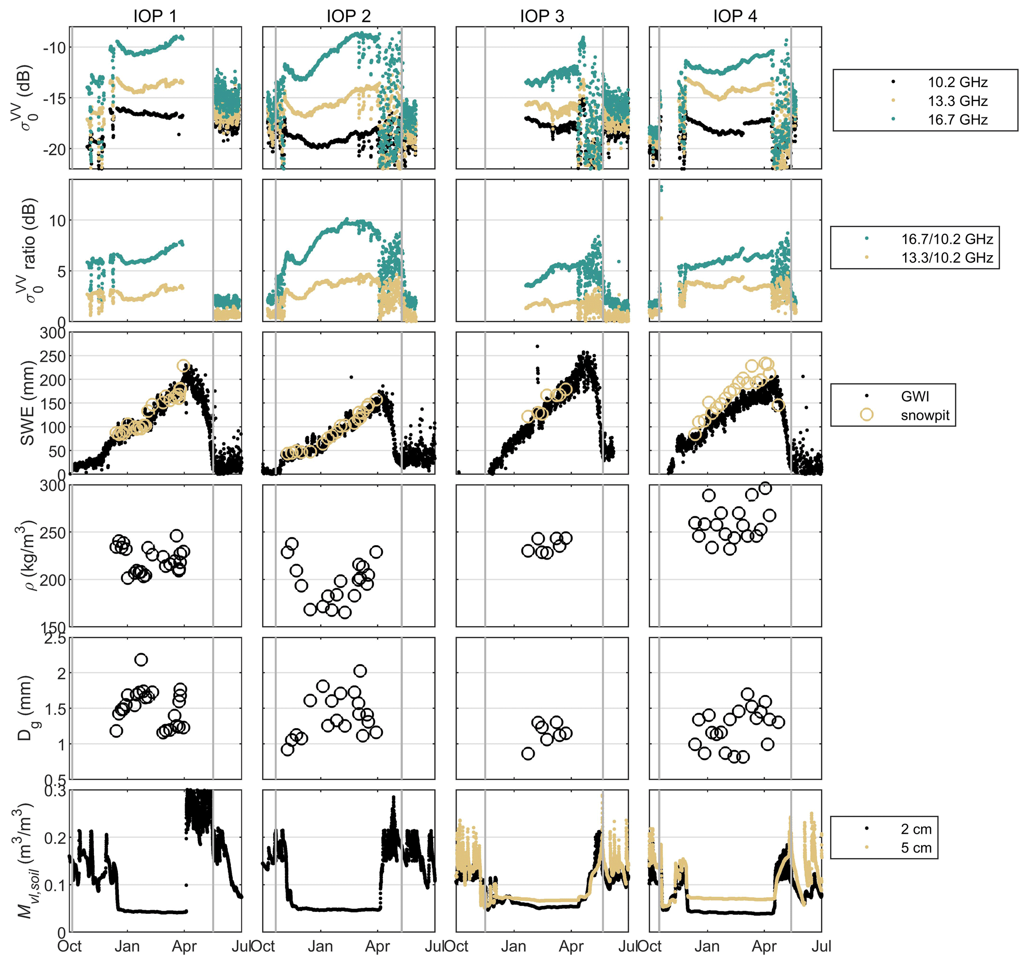
Figure 1 Measured backscattering coefficient at VV polarization (${\mathit{\sigma }}_{\mathrm{0}}^{\mathrm{VV}}$) and snow parameters in four IOPs in NoSREx. The first row shows ${\mathit{\sigma }}_{\mathrm{0}}^{\mathrm{VV}}$ at three frequencies at a 50° incidence angle. The second row shows the ratio of ${\mathit{\sigma }}_{\mathrm{0}}^{\mathrm{VV}}$ between two frequencies. The third row shows the snow water equivalent (SWE). The fourth row shows the profile-average snow density weighted by snow mass (ρ). The fifth row shows the profile-average geometric grain size weighted by snow mass (D_g). The sixth row shows the measured liquid water content (M_vl,soil) by the Delta-T Devices ML2x sensor (at 2 cm) and the Decagon 5TM sensors (at 5 cm). The circles represent measurements from snowpits for SWE, ρ, and D_g. Gray vertical bars indicate the onset and end of snow season, identified according to snow depth measurements.

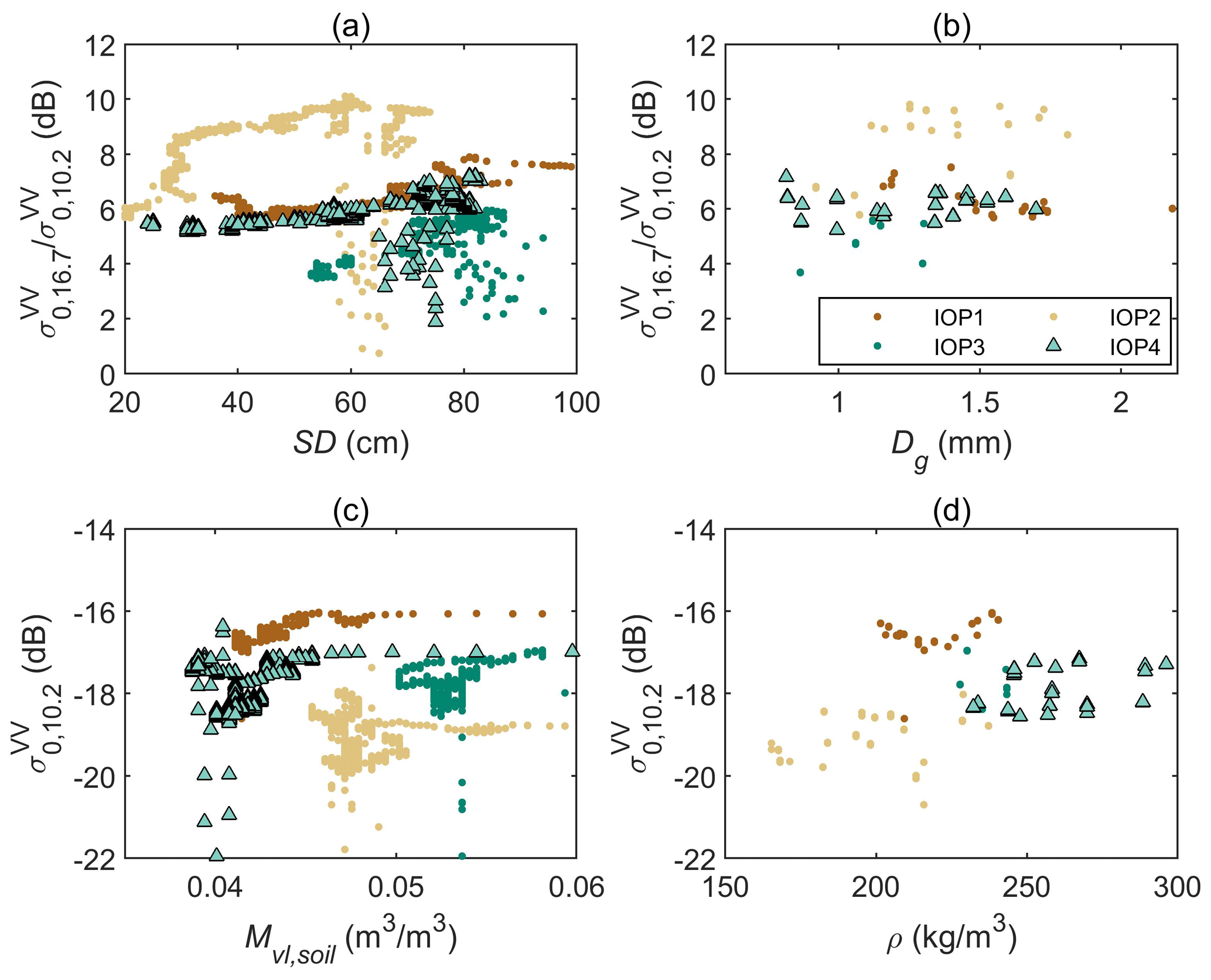
Figure 2 Relationships of the measured backscatter signals with the snow and soil parameters: the measured backscattering ratio between 16.7 and 10.2 GHz, vs. snow depth (SD) (a) and geometric grain size (D_g) (b), respectively; the measured backscattering coefficient at 10.2 GHz in frozen soil period vs. soil liquid water content (M_vl,soil) in (c) and snow density (ρ) in (d), respectively. All data presented here require a soil temperature <0 °C at 2 cm.

3 Methods

3.1 The Markov Chain Monte Carlo method

In this paper, we adapted the Bayesian-based Algorithm for SWE Estimation (BASE), used for inverting passive microwave radiometer measurements in Pan et al. (2017), to radar data. The Markov Chain Monte Carlo (MCMC) method (Gelman et al., 2003) is a numerical realization of the Bayes theorem. Starting from a prior distribution of predicted variables, MCMC randomly searches within the minimum to maximum range of each variable and picks estimates that are both close to the prior and to the observations through the radiative transfer model. The likelihood ratio (R) is used to assess the relative proximity of two sets of SWE and soil parameters to the prior and the observations:

$$\begin{array}{}\text{(1)}& R={\displaystyle \frac{P_{\mathrm{obs}}\left(M\left(x_{i+\mathrm{1}}\right)\right)P_{\mathrm{pr}}\left(x_{i+\mathrm{1}}\right)}{P_{\mathrm{obs}}\left(M\left(x_i\right)\right)P_{\mathrm{pr}}\left(x_i\right)}},\end{array}$$

where x_i is the first set of predicted variables and x_i+1 is the second set. P_pr(x_i) and P_pr(x_i+1) are the probability of x_i and x_i+1 according to the prior distribution. M is the MEMLS3&a observation model, and P_obs(M(x_i)) and P_obs(M(x_i+1)) are the probability of model-simulated backscattering coefficients, M(x_i) and M(x_i+1), according to a normal distribution centered at the observed backscattering coefficients, with a standard deviation of 0.5 dB at each frequency and zero covariance between different frequencies.

At each iteration, if the MCMC algorithm tries to change the value of an estimated variable from x_i to x_i+1, the likelihood ratio, R, is calculated. If R is larger than 1 or larger than a uniformly distributed random threshold R_c between 0 and 1, the change will be accepted; otherwise, it will be rejected. The randomness in R_c is used to prevent local optimization. Finally, all the iterations will build a vector for each estimate variable, which is called the MCMC chain. The MCMC chain is the numerical realization of the posterior distribution, from which we can calculate the final retrieval results and their uncertainties using the mean and the standard deviation.

The MCMC applied here differs from that of Pan et al. (2017) in the following aspects:

1. The observations and observation model were changed from passive to active (radiometer brightness temperature to radar backscatter).

2. We used basically the same generic prior for SWE estimation in Pan et al. (2017). However, the prior distributions were changed from lognormal distributions to normal distributions, because a lognormal-distributed prior leads to a lognormal-distributed posterior distribution, which has a skewness that is challenging to interpret.

3. Snow layer thicknesses were independently estimated in Pan et al. (2017), whereas in this study, we estimate the bottom-layer thickness and the relative ratio of the surface layer thickness to the bottom-layer thickness. This is needed because we found that the radar at these frequencies has a small sensitivity to volume scattering from the surface snow layers of small grain sizes. The use of the layer thickness ratio predetermined the existence of the surface layer and it was assumed to follow N(1,0.2). In addition, we constrained the density and temperature of the surface layer to be lower than those of the bottom layer. These constraints were realized by dynamically using the bottom-layer density and temperature to be the upper limits of those in the surface layer at each iteration. They were set according to a taiga snow type simply for producing a more reasonable profile feature for these two parameters which are not very sensitive to backscattering observations. Therefore, these constraints can be revised or deleted if detailed prior knowledge is provided.

As a summary, Fig. 3 shows a flowchart of the retrieval algorithm. We refer to this algorithm as BASE-AM (active microwave). As in Pan et al. (2017), the algorithm runs 20 000 iterations, with a burn-in period of 5000. The burn-in period was used to allow the variables to walk from the initial status to a status that can stably reproduce the observation. The final retrieval results were averaged from the MCMC estimates between the 5001 and 20 000 iterations.

Figure 3 A flowchart of BASE-AM.

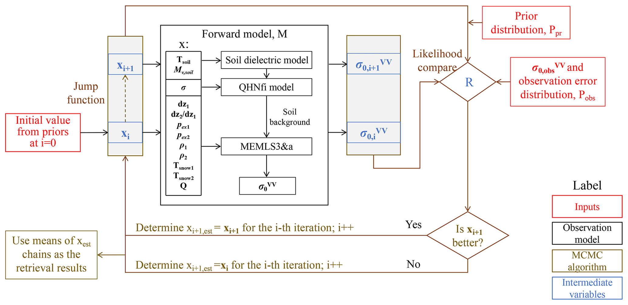
Table 1 provides a comprehensive list of variables estimated in the MCMC algorithm, along with their respective priors. The snow and soil priors are generally aligned with the generic prior used in Pan et al. (2017) at the same site. The main distinction lies in the standard deviations of priors, which were halved compared with those of Pan et al. (2017). This adjustment was made because the boundaries of normal distributions are less constrained than lognormal distributions. As in Pan et al. (2017), the SWE prior was a multiple-year average of monthly-mean SWEs from global 2° resolution VIC model simulations (Nijssen et al., 2001). The snow density and snow temperature priors were from the taiga snow type in Sturm's snow classes (Sturm et al., 1995). The prior for snow exponential correlation length was uninformative, following N (0.18 mm, 0.09 mm). It could be interesting to explore the performance using a different uninformative p_ex prior mean, although it is beyond the scope of this paper. The soil temperature prior was set the same as the snow temperature prior. The prior for total soil water content was set to follow N (8 % vol, 4 % vol). The soil roughness prior was set to follow N (1 cm, 0.5 cm).

Table 1 Summary of priors and boundaries for each estimated variable.

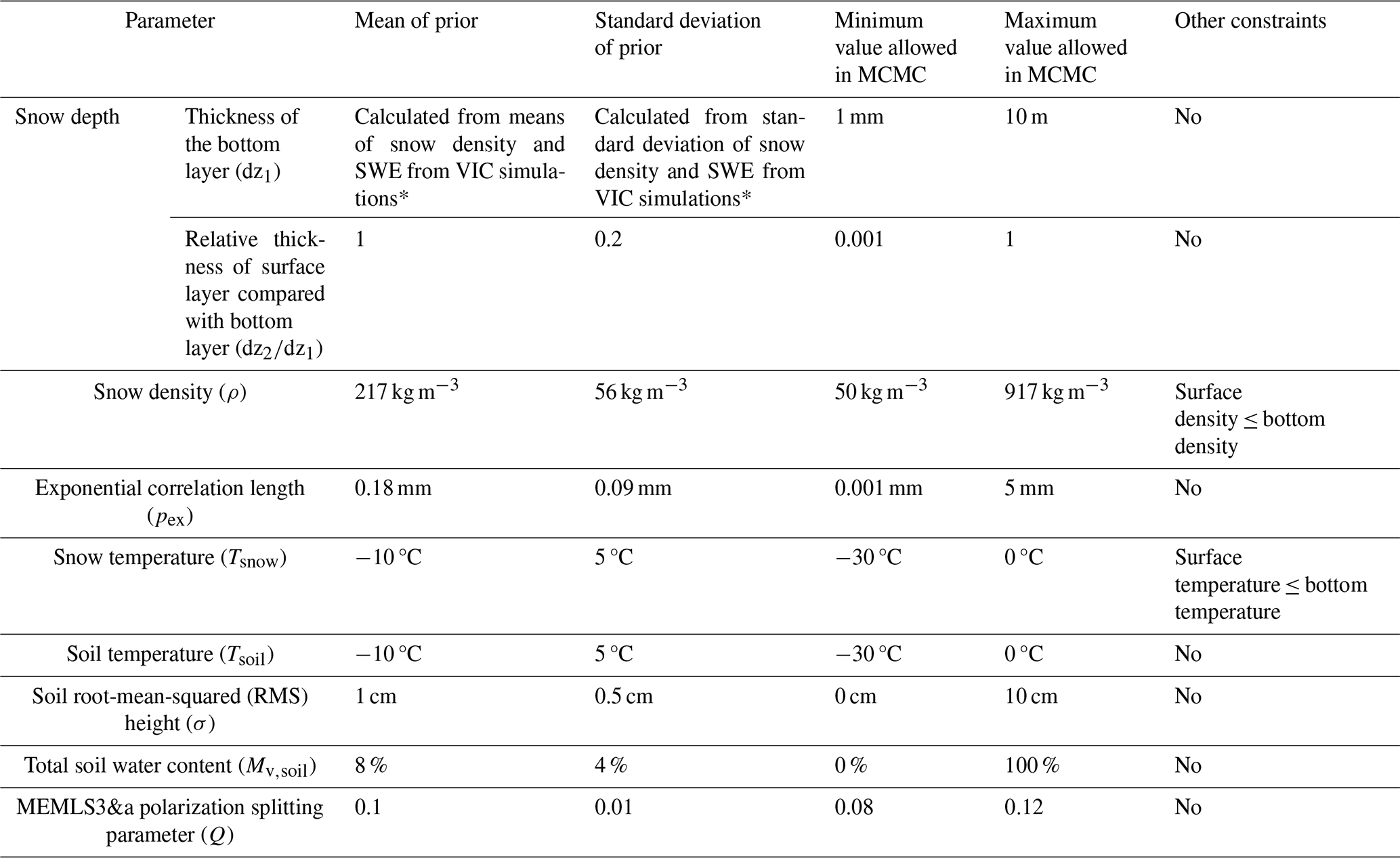
^* The mean of SWE prior is the multiple-year average of the VIC-simulated monthly-mean SWE.

3.2 The MEMLS3&a snow backscattering model

The forward observation model to calculate the snow backscattering was the Microwave Emission Model of Layered Snowpacks 3 and Active (MEMLS3&a) (Proksch et al., 2015) based on the improved Born approximation. MEMLS3&a for active backscattering simulation is a semi-empirical model that converts passive microwave reflectivity of the snowpack to backscattering. It assumes that the distribution of the diffuse part of the bistatic scattering coefficient is Lambertian. In this model, first the snow reflectivity calculated by passive MEMLS (r) is separated into a specular part (r_s) and a diffuse part (r_d). r_s is calculated from the specular part of soil reflectivity, attenuated by snow absorption and snow scattering layer by layer (see Eq. 14 in Proksch et al., 2015). Afterward, $r_{\mathrm{d}}=r-r_{\mathrm{s}}$, and r_d is converted to the diffuse part of the backscattering coefficient (${\mathit{\sigma }}_{\mathrm{d}}^{\mathrm{0}}$) based on the Lambertian assumption as

$$\begin{array}{}\text{(2)}& {\mathit{\sigma }}_{\mathrm{d}}^{\mathrm{0}}=\mathrm{4}{r}_{\mathrm{d}}{\mathit{\mu }}_{\mathrm{0}}^{\mathrm{2}},\end{array}$$

where μ₀ is cos (θ₀) and θ₀ is the incidence angle.

After ${\mathit{\sigma }}_{\mathrm{d}}^{\mathrm{0}}$ is calculated, the specular part of the backscattering coefficient (${\mathit{\sigma }}_{\mathrm{s}}^{\mathrm{0}}$) is calculated using the geometrical optics (GO) theory; ${\mathit{\sigma }}_{\mathrm{s}}^{\mathrm{0}}$ is assumed to be the same for co-polarizations and zero for cross-polarizations, and was calculated from the specular part of reflectivity (r_s) and a roughness parameter (m²) (see Eq. 9 in Proksch et al., 2015). Finally, the total snow backscattering coefficient is calculated as

$$\begin{array}{}\text{(3)}& {\mathit{\sigma }}_{p{p}^{\prime }}^{\mathrm{0}}=\left\{\begin{array}{ll}\left(\mathrm{1}-Q\right){\mathit{\sigma }}_{\mathrm{d},\mathrm{v}}^{\mathrm{0}}+{\mathit{\sigma }}_{\mathrm{s}}^{\mathrm{0}}& p=p^{\prime }=v\\ \left(\mathrm{1}-Q\right){\mathit{\sigma }}_{\mathrm{d},\mathrm{h}}^{\mathrm{0}}+{\mathit{\sigma }}_{\mathrm{s}}^{\mathrm{0}}& p=p^{\prime }=h\\ Q\left({\mathit{\sigma }}_{\mathrm{d},\mathrm{v}}^{\mathrm{0}}+{\mathit{\sigma }}_{\mathrm{d},\mathrm{h}}^{\mathrm{0}}\right)/\mathrm{2}& p\cong p^{\prime }\end{array}\right..\end{array}$$

In MEMLS3&a, there are two empirical parameters. The first one is Q, utilized to split ${\mathit{\sigma }}_{\mathrm{d},\mathrm{v}}^{\mathrm{0}}$ into co-polarizations and cross-polarizations. Our forward simulation test based on snowpit measurements suggested a Q between 0.08 and 0.12 at Sodankylä. Therefore, the prior for Q was set to follow N (0.1, 0.01) in Table 1. The second empirical parameter in MEMLS3&a is the roughness parameter, which is the mean-squared slope (m²), in GO. We fixed m² to a value of 0.01 according to simulations, because we found that it only influences backscattering at very small incidence angles (<30°).

3.3 Soil models

MEMLS3&a requires the total and specular part of soil reflectivity, instead of soil backscattering. We utilized the QHN model with frequency-independent parameters (QHNfi) developed in Montpetit et al. (2015) to calculate the total soil surface reflectivity. The specular part (${\mathrm{\Gamma }}_{\mathrm{p}}^{\mathrm{s}}$) of the soil reflectivity is calculated as follows (Mo et al., 1987; Wegmüller and Mätzler, 1999):

$$\begin{array}{}\text{(4)}& {\mathrm{\Gamma }}_{\mathrm{p}}^{\mathrm{s}}=\left[\left(\mathrm{1}-Q_{\mathrm{s}}\right){\mathrm{\Gamma }}_{\mathrm{p}}^{\ast }+Q_{\mathrm{s}}{\mathrm{\Gamma }}_q^{\ast }\right]\exp \left(-\mathrm{4}{k}^{\mathrm{2}}{\mathit{\sigma }}^{\mathrm{2}}{\cos }^{\mathrm{2}}{\mathit{\theta }}_{\mathrm{1}}\right),\end{array}$$

where ${\mathrm{\Gamma }}_{\mathrm{p}}^{\ast }$ and ${\mathrm{\Gamma }}_q^{\ast }$ are the Fresnel reflectivities, k is the wave number, σ is the soil roughness (RMS height of soil surface), θ₁ is the local incidence angle at the snow–soil boundary, and Q_s is the polarization mixing parameter for soil surface scattering, which is set the same as in QHNfi.

The soil dielectric constants were calculated using a revised generalized refractive mixing dielectric model (GRMDM) (Mironov et al., 2004) adapted for frozen soil. The frozen soil is considered as a mixture of dry solids, bound water, transient water, and ice as in Mironov et al. (2017). The model utilized the same bound water content as in Mironov et al. (2004), whereas it fitted temperature-dependent bound water dielectric constants and other important variables using a frozen soil dataset measured at the Beijing Normal University (see Appendix A). The soil texture was set the same as the measurements from NoSREx (Lemmetyinen et al., 2016a).

4 Results

4.1 MCMC performance for active SWE retrieval

Figures 4–6 use the snowpit measured on 13 March 2012 (hereafter referred to as “pit 49”) during IOP3 as an example to show how MCMC works. Figure 4 shows the simulated backscattering coefficient at each iteration, whereas Figs. 5 and 6 show the variations of all estimated variables at each iteration.

Figure 4 shows that the simulated backscattering coefficients at each iteration in the chain (after the burn-in period) are close to the observations, which is one of the key characteristics of MCMC-based retrieval. The mean bias is 0.23, 0.68, and −0.66 dB at 10.2, 13.3, and 16.7 GHz, respectively. The enlarged subplot of Fig. 4a shows the influence of the initial values of the variables on the first 50 iterations.

Figure 5 shows the MCMC chains (left) and the posterior distributions (right) of the snow variables. The posterior distributions of layer thickness (first row) have lower uncertainty than the priors and the mean is different from that of the prior. For the estimation of exponential correlation length (p_ex) (second row), the BASE-AM algorithm predicts a smaller surface p_ex and a larger bottom-layer p_ex, although the relative relationship between the two layers for p_ex was not constrained. As shown in the width of the posterior distribution, the uncertainty in surface-layer p_ex is larger than that of bottom-layer p_ex. In the third row, the surface-layer snow density is smaller than the bottom-layer density. However, this is simply a realization of our constraint on the relative relationship between the two layers. In the fourth row, the backscattering coefficient is not sensitive to snow temperature, so the posterior distributions of snow temperature highly overlap with the priors. The surface-layer snow temperature was constrained to be lower than that of the bottom layer in MCMC iterations, and it was realized as shown here.

Figure 6 shows the MCMC chains (left) and the posterior distributions (right) of the soil and model variables. The first and fourth rows show that the backscattering coefficient is not sensitive to soil temperature or to the model variable, Q: their posterior distributions follow the prior distributions. The second and third rows show that the algorithm gives a small value for total soil water content, whereas the soil roughness varies. This behavior is not identical among snowpits; the total soil water content can have greater variability than soil roughness. The backscattering coefficient at low frequency in this paper is limited, so the algorithm cannot stably estimate soil roughness and soil moisture variables at the same time. This is discussed in detail in Sect. 5.1.

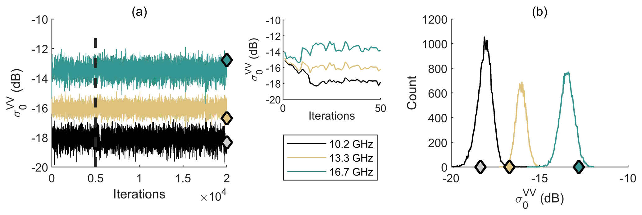
Figure 4 MCMC chain of simulated backscattering coefficients (lines) compared with the measured backscattering coefficients (diamonds) for pit 49: (a) in chains of 20 000 iterations with an enlarged plot on the right showing the first 50 iterations, and (b) in histograms.

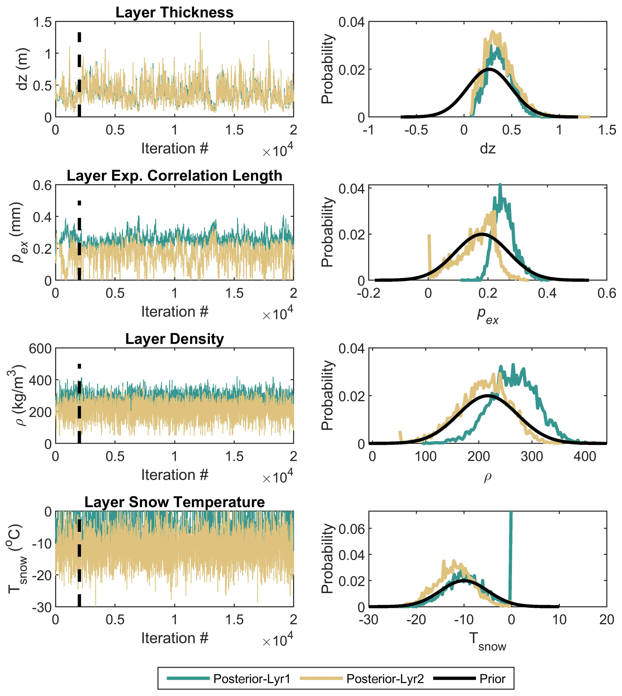
Figure 5 MCMC chain of layered snow properties (first column) and their posterior distributions compared with the prior distributions (second column) for pit 49. Lyr1 is for the bottom layer and Lyr2 is for the surface layer.

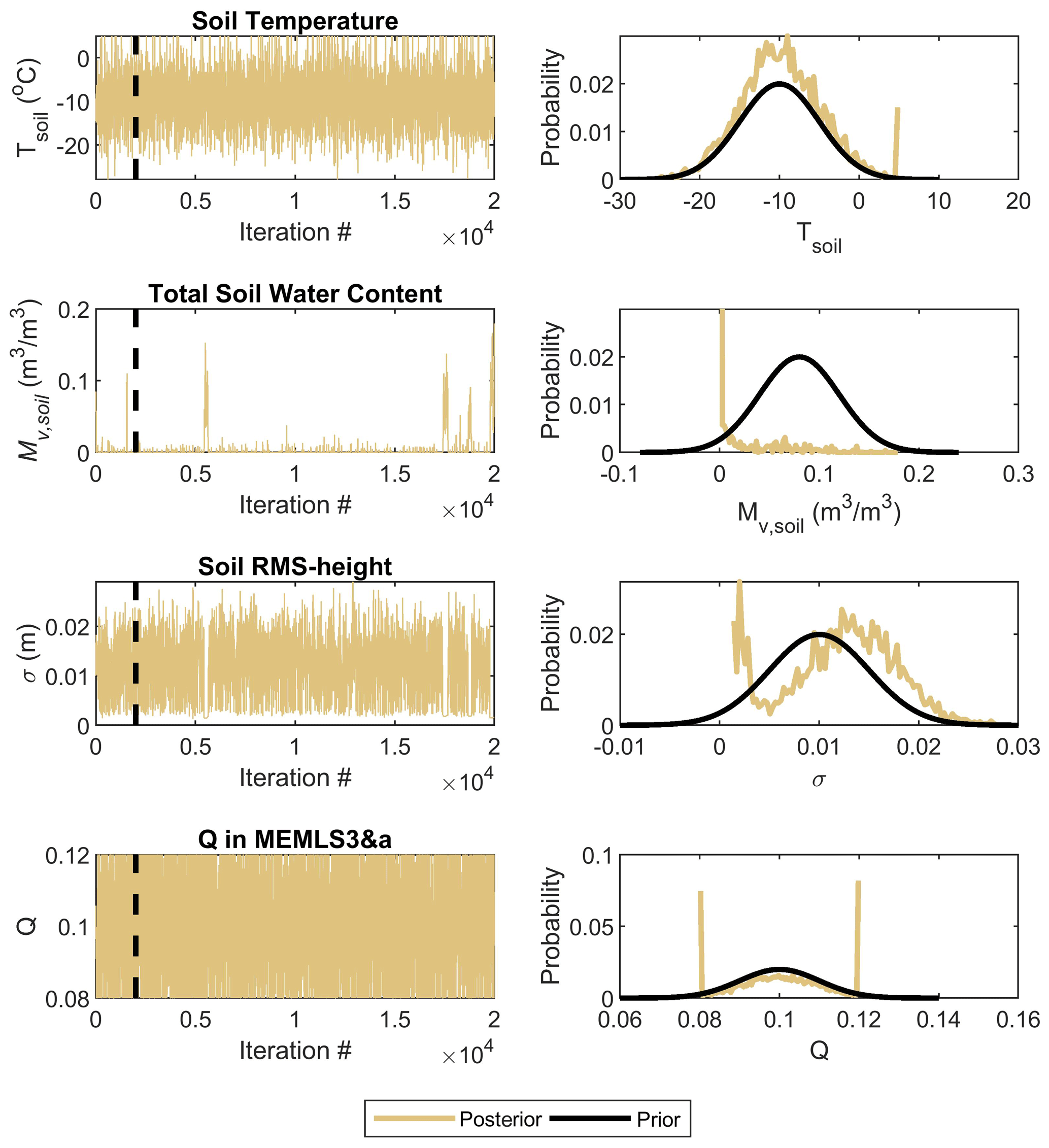
Figure 6 MCMC chain of other soil and model variables (first column) and their posterior distributions compared with the prior distributions (second column) for pit 49.

4.2 Estimation of snow depth and snow water equivalent

Figure 7 shows the MCMC-estimated snow depth (SD) (Fig. 7a) and SWE (Fig. 7b), from the averages of MCMC chains after the burn-in period. The BASE-AM algorithm corrects the underestimation of VIC priors: the original biases for SWE are −49.6, −16.8, −54.5, and −87.9 mm for IOP1, IOP2, IOP3, and IOP4, respectively, whereas the biases are changed to 12.3, 25.8, −15.3, and −34.8 mm, respectively, after retrieval. Figure 8 summarizes the root-mean-squared error (RMSE). On average, the BASE-AM algorithm reduces the posterior RMSE to about half of the prior. The SWE RMSE for all snowpits is within 30 mm, whereas the snow depth (SD) RMSE for all snowpits is close to 10 cm. For IOP2, the RMSE of the posterior SWE is higher than that of the prior SWE because of an overestimation of both SD and snow density. In IOP4, we observe a strong influence of snow density accuracy on SWE retrieval when the SD estimation aligns with the fluctuation of SD caused by snowfall and snow compaction events.

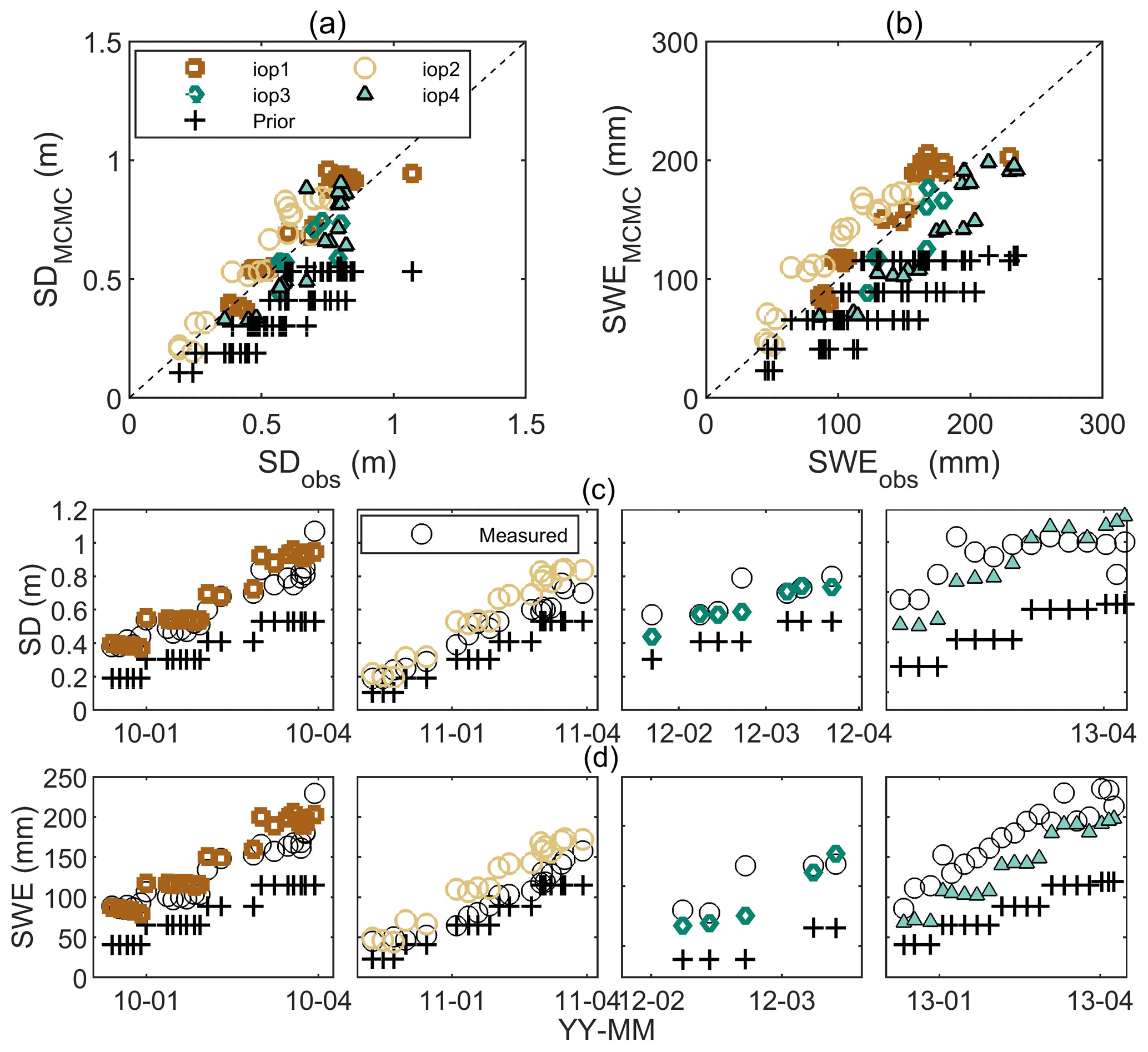
Figure 7 BASE-AM estimated snow depth (SD) versus observed SD at Sodankylä (a, c), and BASE-AM estimated snow water equivalent (SWE) versus observed SWE (b, d). Scatterplots are shown in (a) and (b), and the time series are shown in (c) and (d).

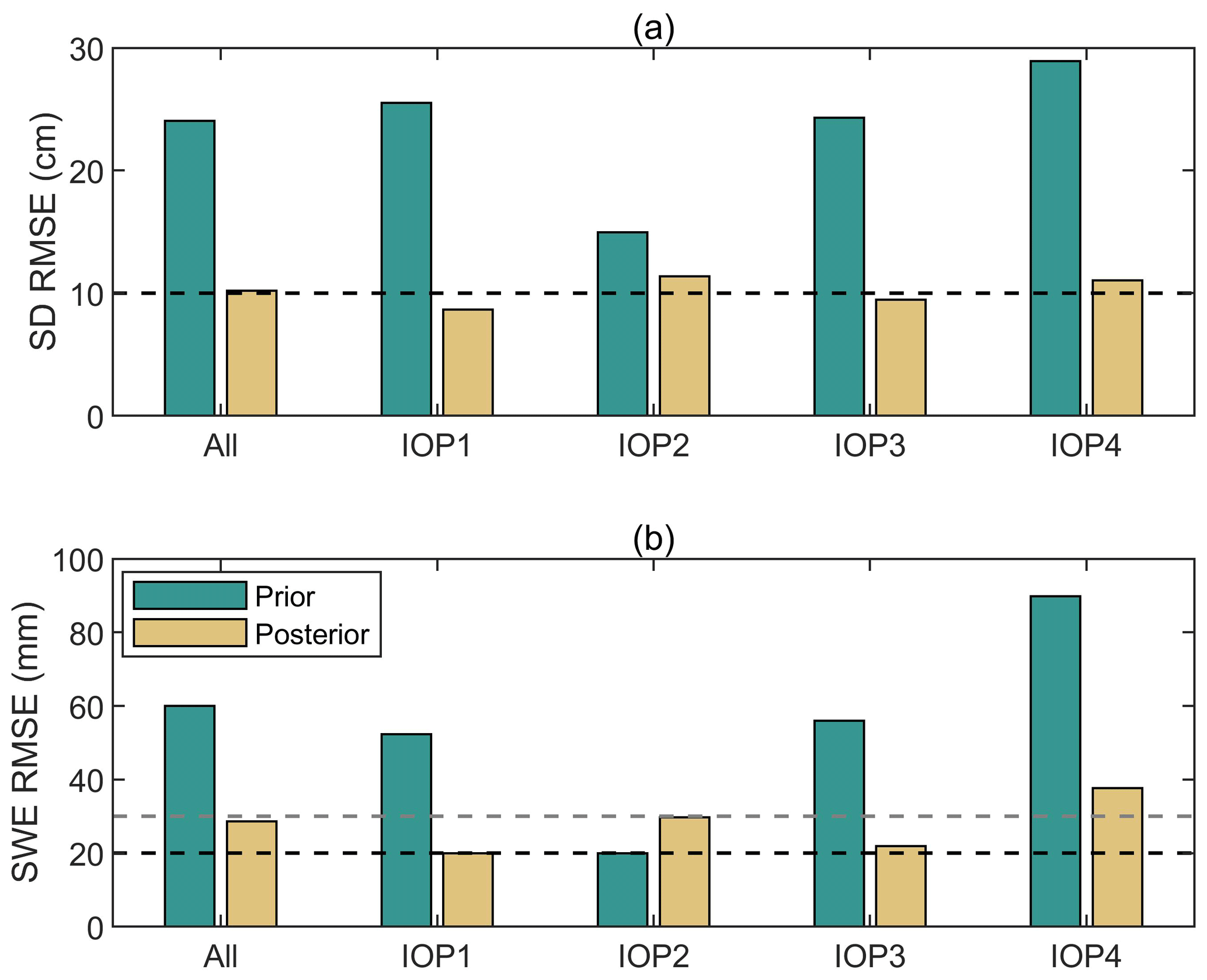
Figure 8 Summary of root-mean-squared error (RMSE) for SD (a) and SWE (b) for different IOPs. The dashed black line in (a) indicates 10 cm RMSE for SD, and the dashed black and gray lines in (b) indicate 20 and 30 mm RMSE, respectively, for SWE.

4.3 Estimation of snow microstructure

Figure 9 shows a comparison between the MCMC-estimated exponential correlation length (p_ex), p_ex converted from the measured D_g using the conversion equation in Pan et al. (2017), as $p_{\mathrm{ex}}=\mathrm{0.227}+\mathrm{0.126}\times \log \left(D_{\mathrm{g}}\right)$, and a p_ex fitted from the backscattering measurements using MEMLS3&a. The fitted p_ex was calculated based on the snowpit and soil measurements, using an adjustable soil roughness (σ) to match the X band and a scaling factor for p_ex to match the other frequencies. Thep_exscaler was constant along the snow profile but varied for different snowpits.

Figure 9a shows that when p_ex converted from measured D_g is high in one IOP, the MCMC-estimated p_ex is also high. However, Fig. 9b shows that within each IOP, the correlation between p_ex converted from D_g measurements and MCMC-estimated p_ex is low. The low correlation results from uncertainties in D_g observation, the D_g−p_ex conversion equation, and probably uncertainties in backscattering observation and MEMLS3&a as well. Figure 9c shows that if p_ex is fitted from radar measurements using the same MEMLS3&a model, it matches significantly better with the MCMC-estimated p_ex. The result in Fig. 9c indicates that BASE-AM may be able to estimate snow microstructure parameter and SWE together if the observation model can accurately describe the relationship between snow–soil parameters and radar measurements.

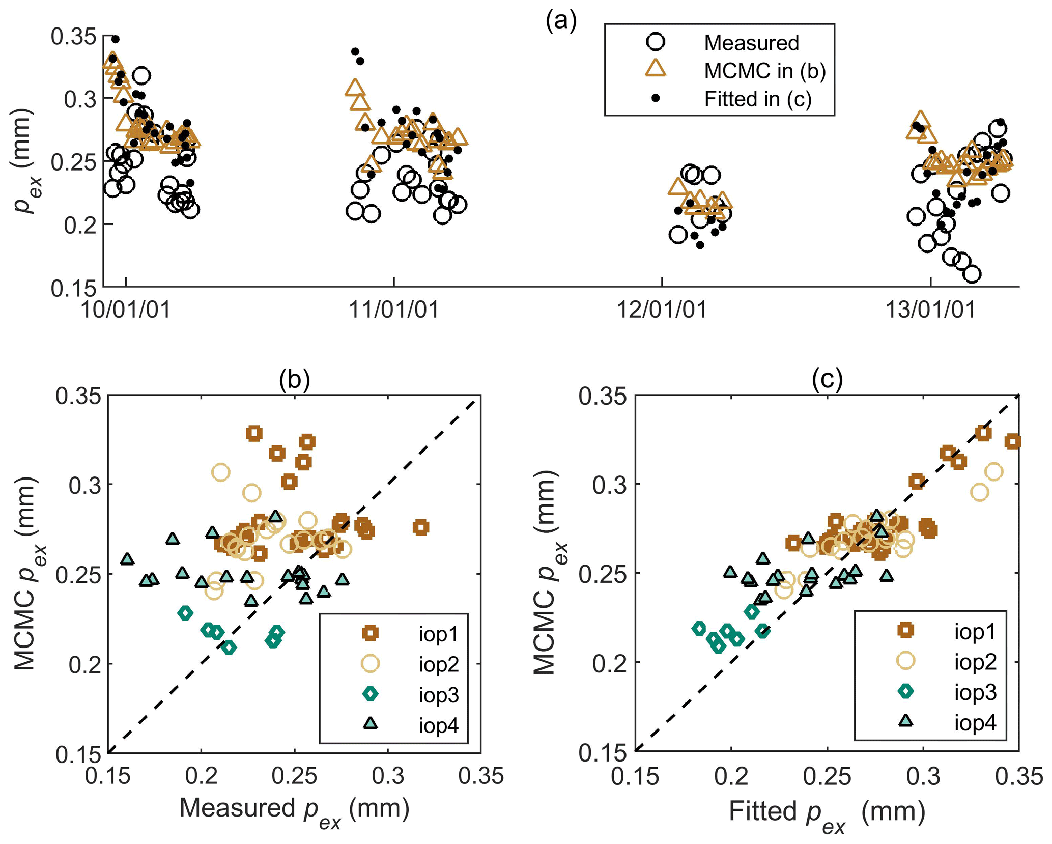
Figure 9 Time series (a) and scatterplots of BASE-AM estimated profile-average exponential correlation length (p_ex) compared with p_ex converted from measured D_g from snowpits in (b), and with the fitted p_ex in (c). The fitted p_ex comes from the use of MRMLS3&a to match the measured backscattering coefficient at three frequencies.

Figure 10 uses 2D distribution maps to show the relationship between layer thickness and exponential correlation length (p_ex) in the MCMC chains, after the burn-in period, for pit 49. After the burn-in period, all combinations of estimated variables can reproduce the observation. Figure 10 shows that the measured backscattering coefficients specify an up–down flipped logarithm-like relationship between layer thickness and p_ex: when layer thickness is high, p_ex is low, and vice versa; both parameters begin to saturate when the other approaches a high value. The area in dark purple is better represented in the MCMC chain and thus has the highest probability, considering both observations and priors. This high-probability area forms a logarithm-shape stripe instead of converging to a single point, indicating that estimating SWE using robust priors requires a global optimization instead of a local optimization. In Fig. 10a and b, the observation changes the priors of layer thickness and p_ex at the intersection of the dashed red lines to the posteriors at the intersection of the dashed black lines. However, in Fig. 10c, there is more uncertainty in the estimation of the surface-layer p_ex than there is in that of the bottom-layer p_ex, because the sensitivity of radar backscatter to volume scattering decreases with decreasing p_ex.

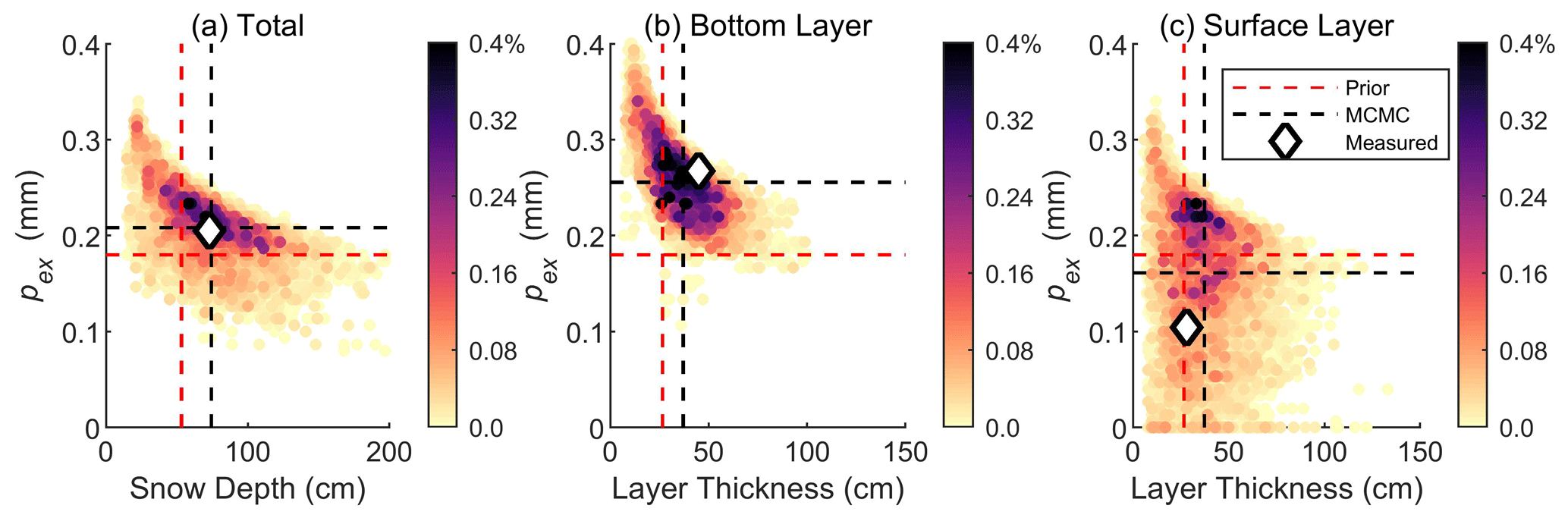
Figure 10 A 2D histogram of probability between layer thickness and exponential correlation length (p_ex) from the MCMC chain after the burn-in period for pit 49: (a) for the entire snowpit, where the snow depth and mass-weighted average p_ex are presented; (b) for the bottom layer; and (c) for the surface layer. The dashed red lines represent the means of priors. The dashed black lines represent the means of posteriors, which are the MCMC retrieval results. The white-face diamonds represent the measured SD (or layer thickness) and p_ex converted from the measured D_g from the snowpit measurements.

5 Discussion

5.1 Concerning snow density, soil roughness, and soil moisture

The backscattering coefficient at 10.2 GHz (${\mathit{\sigma }}_{\mathrm{0}}^{{\mathrm{VV}}_{\mathrm{10.2}}}$) is determined by snow density, soil liquid water content, and soil roughness, and we have shown the sensitivity of ${\mathit{\sigma }}_{\mathrm{0}}^{{\mathrm{VV}}_{\mathrm{10.2}}}$ to the first two variables (see Fig. 1). However, for each snowpit, a single observation of ${\mathit{\sigma }}_{\mathrm{0}}^{{\mathrm{VV}}_{\mathrm{10.2}}}$ is insufficient to determine three variables together. From our retrieval result, we found that regardless of the measured profile-average snow density ranging from 150 to 300 kg m⁻³, the BASE-AM algorithm consistently estimated a snow density of 215.5 kg m⁻³, with a standard deviation of only 7.0 kg m⁻³ across all snowpits. According to our simulations, the sensitivity of the microwave signal to snow density is lower than that of the soil parameters. This indicates that snow density is difficult to retrieve based on a single low-frequency microwave observation, unless soil liquid water content and soil roughness are provided (Gao et al., 2023), or more observations are provided (Lemmetyinen et al., 2016b).

As for the other two soil variables, the results in Sect. 4 are based on the default BASE-AM algorithm configuration to estimate total soil water content and soil roughness simultaneously. To further explore the algorithm, we conducted an additional experiment estimating only the soil moisture using a fixed soil roughness of 1 mm. We found that when both of these soil parameters were estimated, the RMSE of the simulated backscattering coefficient in MCMC (0.43 dB) was closer to the observations (0.52 dB) . In addition, the accuracy of MCMC-estimated SD and SWE is slightly higher, with the RMSEs for all snowpits being 10.2 cm and 28.67 mm, respectively, compared with 10.71 cm and 30.14 mm, respectively. However, Fig. 11 shows that, when the soil roughness is fixed, the temporal variation of estimated soil liquid water content matches better with the sensor measurements, which means the soil liquid water content becomes retrievable. This suggests a possible strategy where the soil roughness is estimated early in the season, and the result would be used for the rest of the period if there is a desire to better estimate soil moisture dynamics from the radar data.

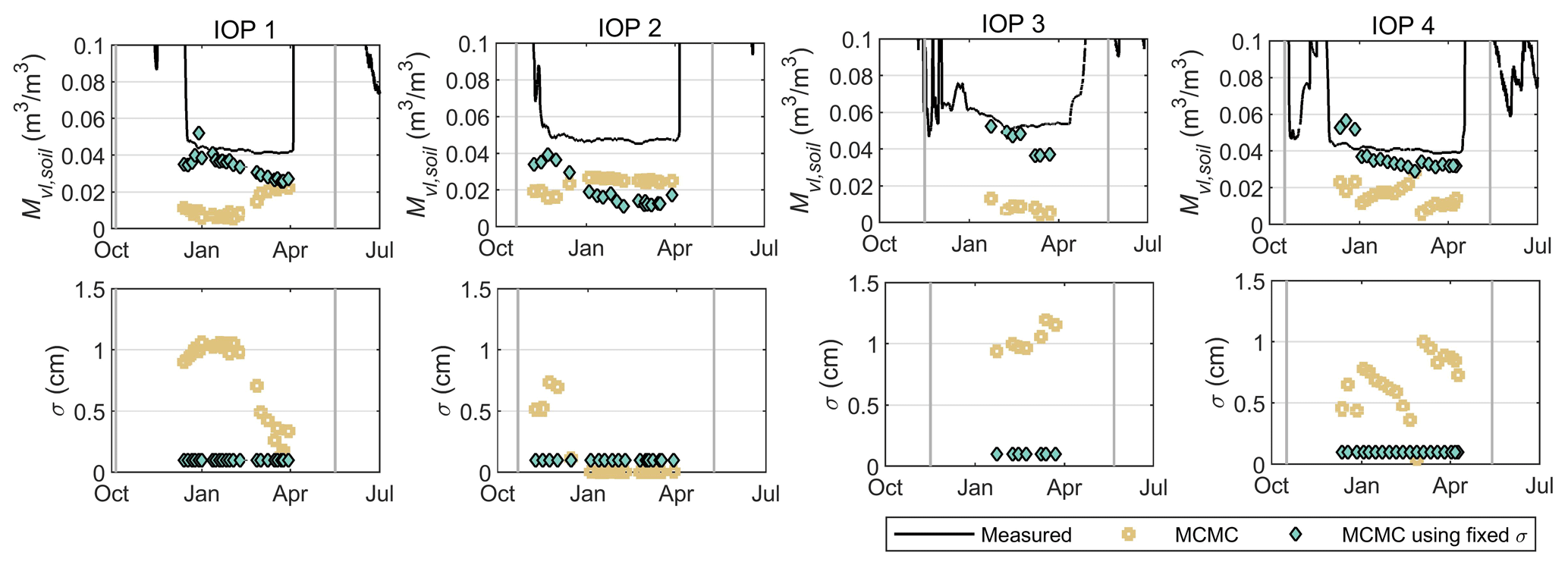
Figure 11 Comparison of MCMC-estimated soil liquid water content (m_vl,soil) and soil roughness (σ) when both soil moisture and soil roughness are estimated (light brown circles) or only soil moisture is estimated (green diamonds). The MCMC m_vl,soil is calculated from the MCMC-estimated total soil water content and soil temperature using the same unfrozen soil water content equation in the forward model.

5.2 The influence of the number of modeled snow layers on the retrieval

Figure 12 shows the MCMC-estimated SD and SWE when the snow is assumed to have a single layer. The same snow and soil priors were used. When the one-layer snow assumption is used, BASE-AM cannot fully correct the underestimation of the SWE prior. This occurred because the presence of a surface snow layer was overlooked. This layer generates very small volume scattering, rendering it nearly transparent to radar. Therefore, it is crucial to acknowledge the existence of such a surface layer; otherwise, the total SD will be underestimated. At the same time, because the equivalent one-layer p_ex represents that from the bottom layer, it will be larger than the profile-average p_ex (from both the D_g measurements and model fittings) (see Fig. 13). As summarized in Table 2, the snow retrieval result using the two-layer assumption has a higher absolute bias and lower RMSE. The one-layer assumption underestimates SD and SWE, and it overestimates profile-average p_ex.

Figure 14 shows a comparison of the SD–p_ex relationship in MCMC chains determined by the same backscattering measurements for pit 49 using different snow layer assumptions. For the one-layer retrievals, the same three-frequency backscattering coefficients determined higher profile-average p_ex. Thus, the snow layer assumption can influence the SD and p_ex estimation results, despite the priors utilized. At the same time, Fig. 14 agrees with the common sense that when more variables are estimated, the uncertainty in the variables increases.

Therefore, as a short summary, we recommend considering two layers since radar tends to overlook the surface snow layer of small grain size. Additionally, based on the balance between the current numbers of radar observations and predicted variables, introducing more layers provides little or no improvements in SWE estimation, unless a reliable prior for snow stratigraphy detail becomes available.

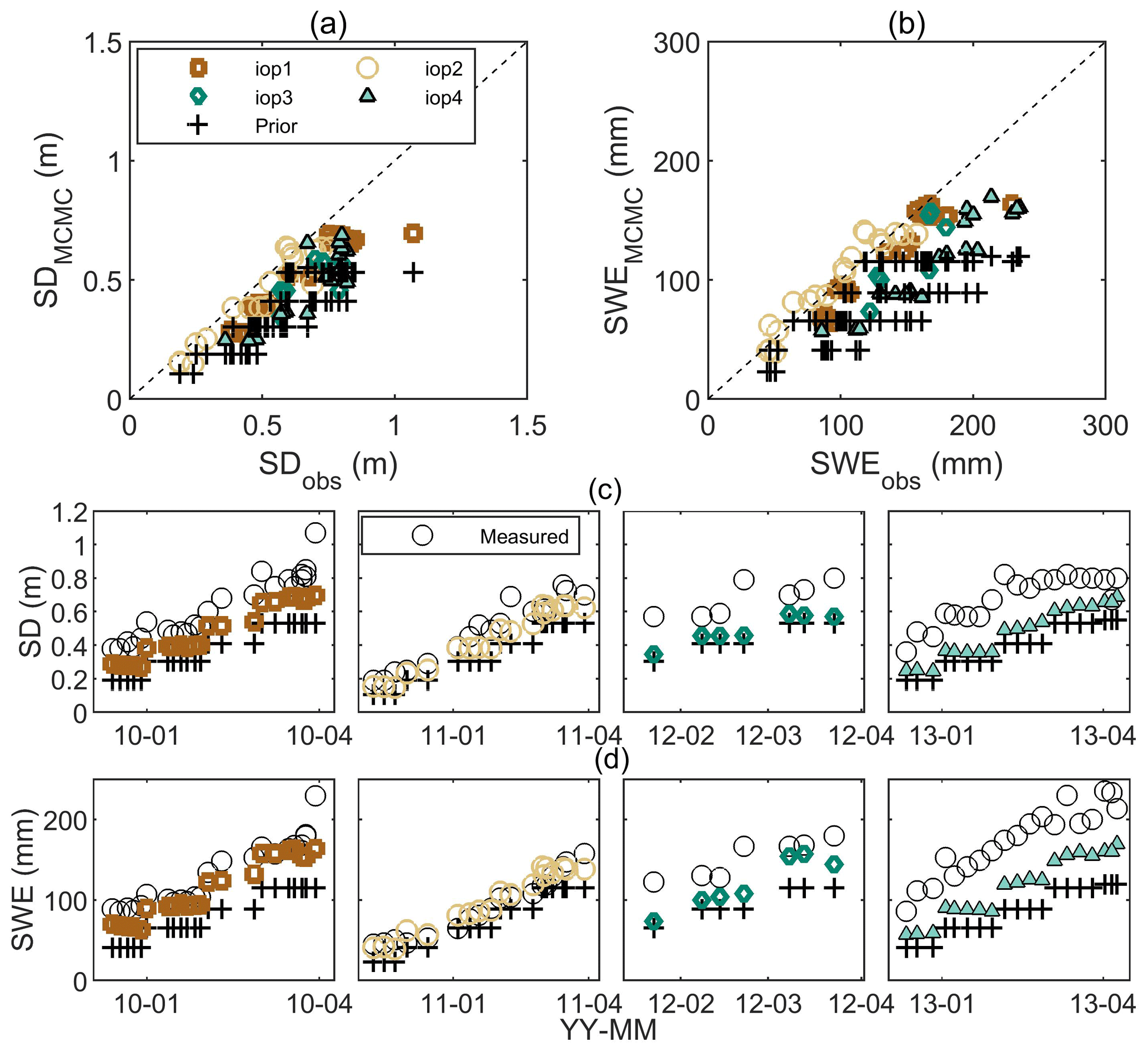
Figure 12 BASE-AM estimated snow depth (SD) (a, c) and snow water equivalent (SWE) (b, d) using the one-layer snow assumption compared with the measurements.

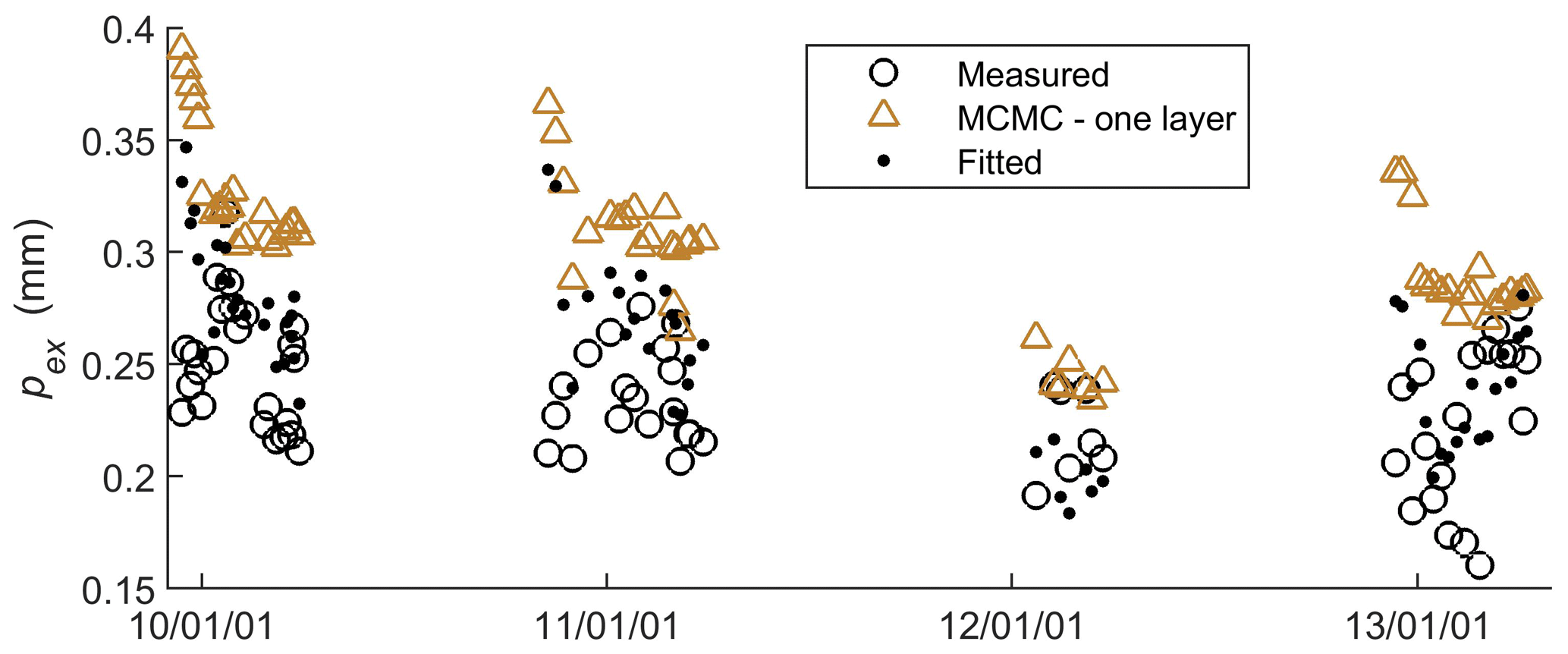
Figure 13 BASE-AM estimated p_ex using the one-layer snow assumption compared with the measurements.

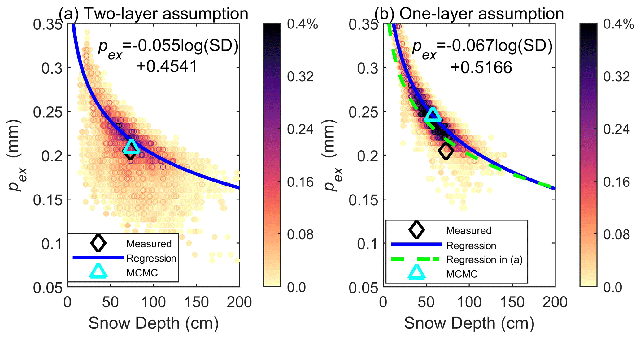
Figure 14 Comparison between the SD and profile-average p_ex relationships in MCMC chains using two-layer (a) and one-layer (b) snow assumptions, respectively, for pit 49. The highest probability point at each SD was calculated and used to fit a logarithmic equation between SD and p_ex, and is labeled as a blue curve in both panels. The equation fitted in (a) is indicated by a dashed green curve in (b) to make a comparison. The measurements are indicated by black diamonds. The MCMC-estimated SD and p_ex are indicated by blue triangles in both panels.

Table 2 Summary of SD, SWE, and profile-average exponential correlation length (p_ex) estimation error using two-layer and one-layer snow assumptions.

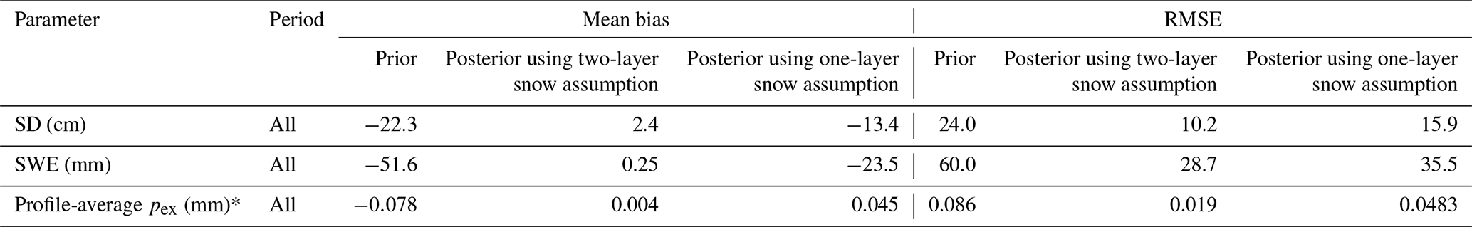
^* To compare with the MCMC p_ex, here we used the fitted p_ex instead of the snowpit-measured p_ex as the reference. The source of the fitted p_ex can be found in Sect. 4.3.

6 Conclusions

In this paper, we developed a Bayesian-based Algorithm for SWE Estimation for Active Microwave (BASE-AM) to retrieve the snow and soil parameters from a site in Sodankylä, Finland, based on X- and dual Ku-band VV polarization backscattering coefficients using biased SWE and uninformative snow microstructure priors. Results show that by predetermining the snowpack to have two layers, SD can be retrieved with an RMSE of 10.2 cm in 0–1 m range, and SWE can be retrieved with an RMSE of 28.7 mm in 0–200 mm range. The radar backscattering observations can correct the bias of SD prior from −22.3 to 2.4 cm using two-layer snow assumptions, but it can be only corrected to −13.4 cm if one-layer snow assumption is used. Results assuming a single layer are significantly less accurate, despite using the same priors.

By iteratively updating several snow and soil variables in the MCMC chain and comparing the prior and posterior distributions, we showed that the key variables required to be estimated in BASE-AM are layer thickness, layer microstructure parameter, and soil liquid water content. The backscattering coefficients in snow and soil are not sensitive to temperature. Backscattering intensity at low frequency is sensitive to snow density, but density cannot be easily retrieved. The polarization splitting parameter (Q) in MEMLS3&a can be fixed unless cross-polarization backscattering observations are introduced.

Overall, our results indicate that active remote sensing observations coupled with generic priors and a two-layer retrieval scheme can support estimation of SWE. Moreover, it is essential to note that the setting of the prior is not a fixed component of the MCMC algorithm. For application in other regions, additional research may be necessary to reset the prior for Q and the relative thickness between two snow layers. For instance, observations of depth hoar in tundra snow types indicate that it occupies only one-third of the entire snow depth and can be adjusted accordingly (King et al., 2018; Saberi et al., 2021). Snow stratigraphy from in situ measurements or multiple-layer snow process model simulations (Pan et al., 2023) can also be incorporated to improve the retrieval performance. However, the example presented in this paper is currently computationally expensive, limiting its feasibility for generating products at a global scale. For global application, firstly, we can reduce the number of predicted variables. For instance, snow and soil temperatures can be replaced with predictions from a land surface model. Soil roughness can be predetermined during snow-free periods, as shown in the example in Gao et al. (2023). For snow density and soil moisture, methods like those in Zhu et al. (2018) can be employed to avoid solving for both, or knowledge from one can be introduced to solve for the other (Kumawat et al., 2022; Gao et al., 2023). Ideally, the system would only need to iterate the layer thicknesses and layered snow microstructures, with the MCMC algorithm seeking global optimization instead of local optimization. Secondly, the length of chains can be reduced by monitoring the convergence of estimated variables as outlined in Sect. 7.3 of Pan et al. (2017). Thirdly, the computation of scattering coefficients in MEMLS3&a based on IBA can be accelerated by using a machine learning model.

Appendix A: The soil dielectric constant model

The soil dielectric constant model utilized in this paper was developed from the Mironov et al. (2004) model and revised according to the soil dielectric constant measurement experiment conducted by Jinmei Pan using the Agilent vector network analyzer at the Beijing Normal University in China. An introduction of the experiment can be found in Wu et al. (2022). Here, a brief introduction of this model is provided (with more details to be published at a later date). The measurements utilized to develop this model cover a wider soil texture than that in Wu et al. (2002), from loamy sand (77.27 % sand, 16.02 % silt, and 6.71 % clay) to silty clay loam (17.49 % sand, 49.68 % silt, and 32.82 % clay). The gravimetric soil water content of all samples varies from 3 % to 60 % and the soil temperature varies from −30 to 20°C. Soil dielectric constants were measured from 200 MHz to 20 GHz continuously at 200 MHz steps.

Table A1 Sources or equations of ε₀, ε_∞, τ, and σ for different soil water components.

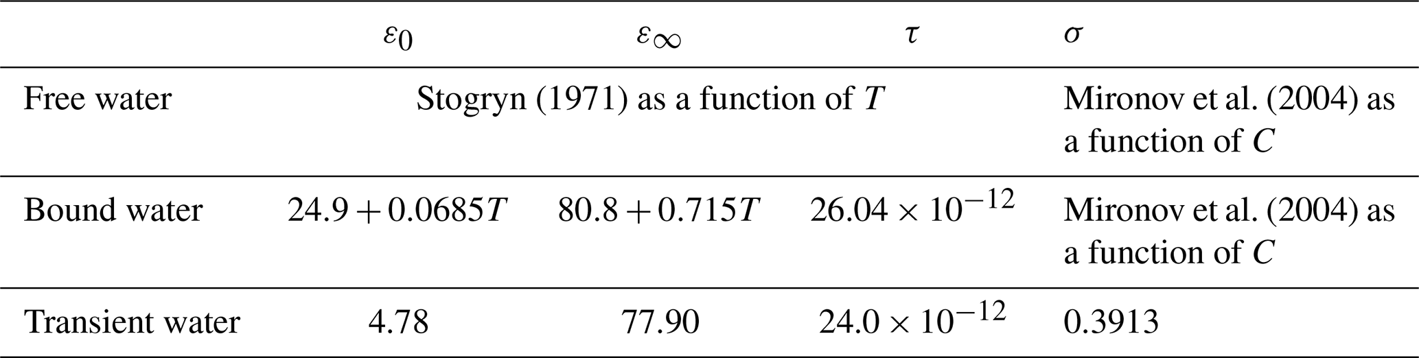
^* T and C are soil temperature (°C) and soil clay content (%).

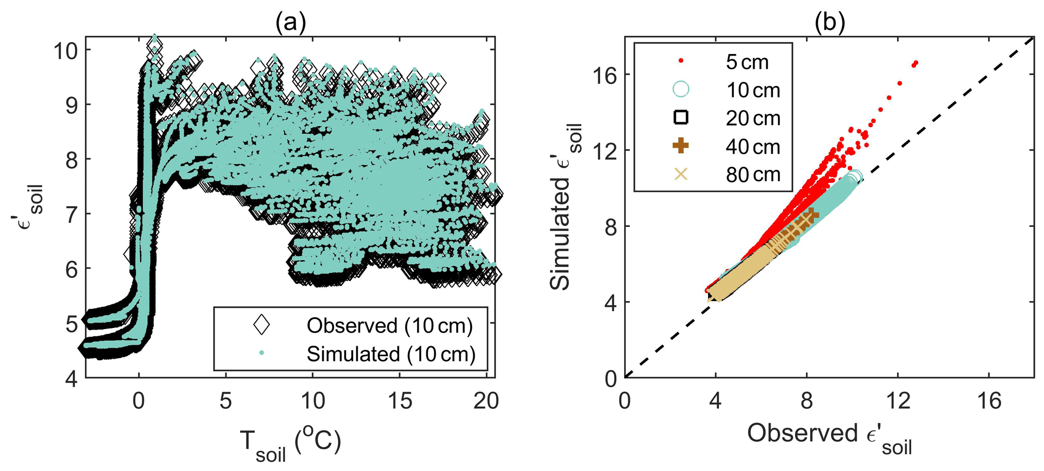
Figure A1 Simulated and observed real part of soil dielectric constants (${\mathit{\epsilon }}_{\mathrm{soil}}^{\prime }$) by the Decagon 5 TM sensor at 100 MHz: (a) sensitivity to temperature for soil measured at 10 cm and (b) scatterplots for soil measured at different depths.

The real and imaginary part of the squared root of soil dielectric constants (ε_soil) are the refractive index (RI) (n) and the normalized attenuation coefficient (NAC) (κ):

$$\begin{array}{}\text{(A1)}& n+i\mathit{\kappa }=\sqrt{{\mathit{\epsilon }}_{\mathrm{soil}}}={\mathit{\epsilon }}_{\mathrm{soil}}^{\prime }+i{\mathit{\epsilon }}_{\mathrm{soil}}^{\prime \prime }.\end{array}$$

n and κof thaw soil are modeled as follows (Mironov et al., 2004):

$$\begin{array}{}\text{(A2)}& {\displaystyle }{n}_{\mathrm{s}}=\left\{\begin{array}{ll}{n}_{\mathrm{d}}+\left(n_{\mathrm{b}}-\mathrm{1}\right)W,& W\le W_{\mathrm{B}}\\ n_{\mathrm{d}}+\left(n_{\mathrm{b}}-\mathrm{1}\right)W_{\mathrm{B}}+\left(n_{\mathrm{u}}-\mathrm{1}\right)\left(W-W_{\mathrm{B}}\right),& W\ge W_{\mathrm{B}}\end{array}\right.\text{(A3)}& {\displaystyle }{\mathit{\kappa }}_{\mathrm{s}}=\left\{\begin{array}{ll}{\mathit{\kappa }}_{\mathrm{d}}+{\mathit{\kappa }}_{\mathrm{b}}W,& W\le W_{\mathrm{B}}\\ {\mathit{\kappa }}_{\mathrm{d}}+{\mathit{\kappa }}_{\mathrm{b}}{W}_{\mathrm{B}}+{\mathit{\kappa }}_{\mathrm{u}}\left(W-W_{\mathrm{B}}\right),& W\ge W_{\mathrm{B}}\end{array}\right.,\end{array}$$

where the subscripts n and κ, which include d, b, and u, represent dry soil solids, bound water, and free water, respectively. In the soil–water system, a fraction of bound water, which has a different dielectric property compared with free water, adheres to soil solids. The maximum allowable bound water content is denoted as W_B. If the total water content (W) is lower than W_B, then the model will contain only two components, as indicated by the first lines of Eqs. (A2) and (A3); otherwise, it will contain three components.

n and κ of frozen soil are modeled as follows (Mironov et al., 2017):

$$\begin{array}{}\text{(A4)}& {\displaystyle }{n}_{\mathrm{s}}=\left\{\begin{array}{ll}{n}_{\mathrm{d}}+\left(n_{\mathrm{b}}-\mathrm{1}\right)W,& W\le W_{\mathrm{B}}\\ n_{\mathrm{d}}+\left(n_{\mathrm{b}}-\mathrm{1}\right)W_{\mathrm{B}}+\left(n_{\mathrm{t}}-\mathrm{1}\right)\left(W-W_{\mathrm{B}}\right),& W_{\mathrm{B}}\le W\le W_{\mathrm{U}}\\ n_{\mathrm{d}}+\left(n_{\mathrm{b}}-\mathrm{1}\right)W_{\mathrm{B}}+\left(n_{\mathrm{t}}-\mathrm{1}\right)\left(W_{\mathrm{U}}-W_{\mathrm{B}}\right)& \\ +\left(n_{\mathrm{i}}-\mathrm{1}\right)\left(W-W_{\mathrm{U}}\right),& W\ge W_{\mathrm{U}}\end{array}\right.\text{(A5)}& {\displaystyle }{\mathit{\kappa }}_{\mathrm{s}}=\left\{\begin{array}{ll}{\mathit{\kappa }}_{\mathrm{d}}+{\mathit{\kappa }}_{\mathrm{b}}W,& W\le W_{\mathrm{B}}\\ {\mathit{\kappa }}_{\mathrm{d}}+{\mathit{\kappa }}_{\mathrm{b}}{W}_{\mathrm{B}}+{\mathit{\kappa }}_{\mathrm{t}}\left(W-W_{\mathrm{B}}\right),& W_{\mathrm{B}}\le W\le W_{\mathrm{U}}\\ {\mathit{\kappa }}_{\mathrm{d}}+{\mathit{\kappa }}_{\mathrm{b}}{W}_{\mathrm{B}}+{\mathit{\kappa }}_{\mathrm{t}}\left(W_{\mathrm{U}}-W_{\mathrm{B}}\right)+{\mathit{\kappa }}_{\mathrm{i}}\left(W-W_{\mathrm{U}}\right),& W\ge W_{\mathrm{U}}\end{array}\right.,\end{array}$$

where the subscripts n and κ, which include d, b, t, and i, represent dry soil solids, bound water, transient water, and ice, respectively. Soil solids and bound water have the same physical meanings for frozen soil and thaw soil. When soil temperature decreases from above-zero degrees Celsius to sub-zero degrees Celsius, not all water will immediately turn to ice. The total volumetric fraction of unfrozen water is called the unfrozen water content (W_U), which can be calculated as a function of temperature and clay fraction. We followed the setting in Mironov et al. (2017) that the bound water will not freeze, and the unfrozen soil water that exceeds the bound water is considered as the transient water.

The key to the soil dielectric constant model is to model W_B, W_U, as well as n and κ for all components. We utilized the same W_B and the same n and κ for soil solids as a function of clay fraction as reported in Mironov et al. (2004). The n and κ of ice refer to the temperature-dependent equation utilized in MEMLS3&a.

The dielectric constants of water components can be modeled by Debye's equation as

$$\begin{array}{}\text{(A6)}& \mathit{\epsilon }={\mathit{\epsilon }}_{\mathrm{\infty }}+{\displaystyle \frac{{\mathit{\epsilon }}_{\mathrm{0}}-{\mathit{\epsilon }}_{\mathrm{\infty }}}{\mathrm{1}-i\mathrm{2}\mathit{\pi }f\mathit{\tau }}}+i{\displaystyle \frac{\mathit{\sigma }}{\mathrm{2}\mathit{\pi }f{\mathit{\epsilon }}_r}},\end{array}$$

where ε_∞ is the dielectric constant in the high-frequency limit, ε₀ is the static dielectric constant in the low-frequency limit, f is the frequency (Hz), τ is the relaxation time (s), σ is the effective conductivity (S m⁻¹), and ε_r is the dielectric constant for free space (8.854 × 10⁻¹² F m⁻¹). Later, ε can be transferred to n and κ using Eq. (A1).

For each component, it is required to determine ε₀, ε_∞, τ, and σ. We adapted some existing equations from Mironov et al. (2004) and Stogryn (1971), and we fitted the remaining parameters according to measurements. We utilized the samples with W<W_B to fit temperature-dependent bound water parameters (see Table A1) and then iteratively fit W_u and transient water parameters using the MCMC approach. Table A1 lists the details of the water component models, and W_U was determined as

$$\begin{array}{ll}\text{(A7)}& {\displaystyle }& {\displaystyle }{W}_{\mathrm{U}}=min\left(A\times {\left|T\right|}^B,W\right){\displaystyle }& {\displaystyle }A=a_{c}C+a_{\mathrm{mv}}W\\ {\displaystyle }& {\displaystyle }B=b_{c}C+b_{\mathrm{mv}}W,\end{array}$$

where C is soil clay content (%), T is soil temperature (°C), a_c=0.00306, a_mv=0.394, b_c=0.00582, and $b_{\mathrm{mv}}=-\mathrm{1.073}$.

Figure A1 shows an example of the model utilized to predict the measured soil permittivity (real part of dielectric constants) at 100 MHz by the Decagon 5 TM sensor in Sodankylä. The simulation utilized the measured liquid water content and measured soil texture. The total soil water content comes from the measured liquid water content before freezing. To calculate soil permittivity, we used a fully independent model as compared with the Decagon 5 TM sensor. Figure A1a shows that our model is able to predict the change in soil permittivity with changes in soil temperature. Figure A1b shows that the simulated soil permittivity is highly consistent with the observations at 10–80 cm depth below the soil surface. The mean bias is 0.0838, with an RMSE of 0.0569. In addition, the model overestimates the measured permittivity for the single top layer at 5 cm, which is influenced by air above the soil and also organic matter. Including the 5 cm layer, the mean bias is 0.129 with an RMSE of 0.198. It indicates that the soil dielectric constant model described here is suitable to be used as part of the forward model described in this paper.