the Creative Commons Attribution 4.0 License.
the Creative Commons Attribution 4.0 License.
 | 12 Mar 2024
Understanding the influence of ocean waves on Arctic sea ice simulation: a modeling study with an atmosphere–ocean–wave–sea ice coupled model
Chao-Yuan Yang
Jiping Liu
Dake Chen
Rapid decline in Arctic sea ice has created more open water for ocean wave development and highlighted the importance of wave–ice interactions in the Arctic. Some studies have made contributions to our understanding of the potential role of the prognostic floe size distribution (FSD) in sea ice changes. However, these efforts do not represent the full interactions across atmosphere, ocean, wave, and sea ice. In this study, we implement a modified joint floe size and thickness distribution (FSTD) in a newly developed regional atmosphere–ocean–wave–sea ice coupled model and conduct a series of pan-Arctic simulations with different physical configurations related to FSD changes, including FSD-fixed, FSD-varied, lateral melting rate, wave-fracturing formulation, and wave attenuation rate. Firstly, our atmosphere–ocean–wave–sea ice coupled simulations show that the prognostic FSD leads to reduced ice area due to enhanced ice–ocean heat fluxes, but the feedbacks from the atmosphere and the ocean partially offset the reduced ice area induced by the prognostic FSD. Secondly, lateral melting rate formulations do not change the simulated FSD significantly, but they influence the flux exchanges across atmosphere, ocean, and sea ice and thus sea ice responses. Thirdly, the changes in FSD are sensitive to the simulated wave height, wavelength, and wave period associated with different wave-fracturing formulations and wave attenuation rates, and the limited oceanic energy imposes a strong constraint on the response of sea ice to FSD changes. Finally, our results also demonstrate that wave-related physical processes can have impacts on sea ice changes with the constant FSD, suggesting the indirect influences of ocean waves on sea ice through the atmosphere and the ocean.
- Article
(16475 KB) - Full-text XML
-
Supplement
(3069 KB) - BibTeX
- EndNote


Arctic sea ice, a major component in the climate system, has undergone dramatic changes over the past few decades associated with global climate change. September and March Arctic sea ice extent show decreasing trends of −13.1 % and −2.6 % per decade from 1979 to 2020, respectively (Perovich et al., 2020). The mean Arctic sea ice thickness has decreased by ∼ 1.5–2 m from the submarine period (1958–1976) to the satellite period (2011–2018), largely resulting from the loss of multiyear ice (Kwok, 2018; Tschudi et al., 2016). The drifting speed of Arctic sea ice exhibits an increasing trend based on satellite and buoy observations (e.g., Rampal et al., 2009; Spreen et al., 2011; Zhang et al., 2022). As the Arctic Ocean has been dominated by thinner and younger ice, Arctic sea ice is more likely to be influenced by forcings from the atmosphere and the ocean.
Associated with the above Arctic sea ice changes, the Arctic fetch (open-water area for ocean wave development) is less limited by the ice cover. Previous studies suggested that the Arctic fetch and surface wind speed over the ice-free ocean correlate well with wave heights in the Arctic Ocean (Casas-Prat and Wang, 2020; Dobrynin et al., 2012; Liu et al., 2016; Stopa et al., 2016; Waseda et al., 2018). The higher ocean waves are more likely to propagate deeper into the ice pack and have sufficient energy to break sea ice into smaller floes (e.g., Kohout et al., 2014). The ice pack, with the same concentration, has larger surface area for the ice floes with smaller sizes, particularly lateral surfaces. The increased lateral surface accelerates ice melting through enhanced ice–ocean heat fluxes (e.g., Steele, 1992). Some studies also showed that the ice-floe melting rate is associated with the horizontal mixing of oceanic heat across the ice-floe edge between open water and under-floe ocean by oceanic eddies, in particular sub-mesoscale eddies, and the strength of this effect depends on floe size (Gupta and Thompson, 2022; Horvat et al., 2016). The enhanced ice melting creates more open water (i.e., fetch), which is a favorable condition for further wave development as well as the ice–albedo feedback (Curry et al., 1995). These processes create a potential feedback loop between ocean waves and sea ice (e.g., Asplin et al., 2014; Thomson and Rogers, 2014).
Arctic cyclones and their high surface wind are the important drivers for large wave events in the Arctic Ocean. Previous studies showed that intense storms like the Great Arctic Cyclone of 2012 (Simmonds and Rudeva, 2012) and a strong summer cyclone in 2016 could be one of the contributors to the anomalously low sea ice extent in 2012 and 2016 (e.g., Lukovich et al., 2021; Parkinson and Comiso, 2013; Peng et al., 2021; Stern et al., 2020; Zhang et al., 2013). Statistical analyses based on cyclone-tracking algorithms across multiple reanalyses suggested that the number of Arctic cyclones shows a significantly positive trend in the cold season (e.g., Sepp and Jaagus, 2011; Valkonen et al., 2021; Zahn et al., 2018). The increased cyclone activities and more open-water areas cause more extreme wave events in the Arctic (e.g., Waseda et al., 2021). Blanchard-Wrigglesworth et al. (2021) found that extreme changes in Arctic sea ice extent are correlated with distinct wave conditions during the cold season based on the observations.
The potential feedback loop associated with ocean waves and sea ice and more extreme wave events indicates the importance of representing these processes in climate models for improving sea ice simulation and prediction (e.g., Collins et al., 2015; Kohout et al., 2014). However, state-of-the-art climate models participating in the latest Coupled Model Intercomparison Project Phase 6 (CMIP6) have not incorporated the interactions between ocean waves and sea ice in their model physics (e.g., Horvat, 2021). The coupled effects of ocean waves and sea ice also include the decay of amplitude of ocean waves as they travel under the ice cover due to a combination of scattering and dissipation. (e.g., Squire, 2020). Crests and troughs of ocean waves exert strains on sea ice, and sea ice breaks if the maximum strain exceeds a certain threshold (e.g., Dumont et al., 2011). The wave-induced ice breaking changes the size of floes, which in turn changes the floe size distribution (FSD; Rothrock and Thorndike, 1984). In addition to the interactions between ocean waves and sea ice, the floe size contributes to the changes in the atmospheric boundary layer (e.g., Schäfer et al., 2015; Wenta and Herman, 2019), mechanical responses of sea ice (e.g., Vella and Wettlaufer, 2008; Weiss and Dansereau, 2017; Wilchinsky et al., 2010), the flux exchanges across air–sea ice–ocean interfaces (Cole et al., 2017; Loose et al., 2014; Lu et al., 2011; Martin et al., 2016; Steele et al., 1989; Tsamados et al., 2014), and the scattering of ocean wave propagation (e.g., Montiel et al., 2016; Squire and Montiel, 2016). Thus, it is essential to have a prognostic FSD to properly reflect wave–ice interactions as well as other processes related to the floe size in climate models.
Recently, several studies have made contributions to understanding responses of sea ice to the prognostic FSD (e.g., Bateson et al., 2020; Bennetts et al., 2017; Boutin et al., 2020; Horvat and Tziperman, 2015; Roach et al., 2018a, 2019; Zhang et al., 2015, 2016). However, these studies used simplified model complexity (i.e., standalone sea ice model, ice–wave coupling, ice–ocean coupling) and were unable to give a full representation of sea ice responses to the evolving states of the atmosphere, ocean, and waves based on explicit model physics as well as feedbacks from sea ice to them. Motivated by this, here we introduce a newly developed atmosphere–ocean–wave–sea ice coupled model, in which we implement physical processes that simulate the evolution of floe size distribution. We use this new coupled model to investigate the responses of sea ice to ocean waves, as well as interactions in the Arctic climate system. This paper is structured as follows. Section 2 provides an overview of the new coupled model, focusing on the wave component and the implementation of the prognostic FSD. Section 3 describes the design of numerical experiments and the related model configurations. Section 4 examines the responses of sea ice to wave–ice interactions with the prognostic FSD, as well as other ocean-wave-related processes. Discussions and concluding remarks are provided in Sect. 5.
The newly developed atmosphere–ocean–wave–sea ice coupled model is based on the Coupled Arctic Prediction System (CAPS; Yang et al., 2022), which consists of the Weather Research and Forecasting (WRF) model, the Regional Ocean Modeling System (ROMS), and the Community Ice CodE (CICE). A detailed description of each model component in CAPS is given in Yang et al. (2020, 2022). In this section, we focus on newly added features in CAPS as described below.
2.1 Wave model component
To represent wave–ice interactions, an ocean wave model is coupled into CAPS, which is Simulating WAves Nearshore (SWAN). SWAN is a third-generation wave model and includes processes of diffraction, refraction, wave–wave interactions, and wave dissipation due to wave breaking, whitecapping, and bottom friction (Booij et al., 1999). Recently, wave dissipation due to sea ice has been implemented in the SWAN model based on an empirical formula, which is called IC4M2 (Collins and Rogers, 2017; Rogers, 2019). Specifically, the temporal exponential decay rate of wave energy due to sea ice is defined as
where Sice is the sink term induced by sea ice, E is the wave energy spectrum, and cg is the group velocity. ki is the linear exponential rate that is a function of frequency as follows:
where c0 to c6 are the user-defined coefficients and their values as described in Sect. 3. In the SWAN model, both the wind source term Sin and the sea ice sink term are scaled by sea ice concentration aice, which is provided by the CICE model through the coupler in CAPS:
2.2 Prognostic FSD
For the prognostic FSD implemented in the CICE model, we follow the joint floe size and thickness distribution (FSTD; Horvat and Tziperman, 2015). FSTD is defined as a probability distribution f(r,h)drdh. f(r,h) represents the fraction of cell covered by ice with floe size between r and r+Δr and thickness between h and h+Δh, and FSTD satisfies
The ice thickness distribution g(h) (ITD; Thorndike et al., 1975), which is simulated by the CICE model, and FSD F(r) can be obtained by integrating FSTD over all floe sizes and all ice thicknesses:
Roach et al. (2018a) suggested the modified FSTD, L(r,h), to preserve the governing equations of ITD in the CICE model, which satisfies
and
As described in Roach et al. (2018a), the implementation of the modified FSTD ignores the two-way relationship between floe size; that is, physical processes associated with FSD changes (i.e., L(r,h) changes) are independent across each ice thickness category. The governing equation of FSTD is defined as
The terms on the right-hand side represent advection, thermodynamics, mechanical, and wave-induced floe-fracturing processes. For these terms, except the last term ℒW, we follow the approach described in Roach et al. (2018a) and related values for coefficients as described in Sect. 3. The formulations of ℒW proposed by Horvat and Tziperman (2015) involve a random function to generate sub-grid-scale sea surface elevation to determine how floes are fractured by ocean waves. As a consequence, simulations are not bitwise reproducible with the formulation including a random function. To avoid this issue, we propose different approaches for our implementation of FSTD as described below.
2.3 Floe fracturing by ocean waves
For the floe-fracturing term ℒW, we follow the formulation suggested by Zhang et al. (2015), which has a similar form to that of Horvat and Tziperman (2015) and can be described as
The first term on the right-hand side represents the areal fraction reduction due to floe fracturing, and the second term is the areal fraction gain from other floe size categories that have floe fracturing. In Eq. (10), Q(r) is the probability that floe fracturing occurs for floe size between r and r+Δr and is the redistributor that transfers fractured floe from floe size r′ to r. ℒW does not create or destroy ice, so it must satisfy
In this study, we propose two different formulations for Q(r) and .
2.3.1 Equal redistribution
We follow the same assumption as in Zhang et al. (2015). That is, ice fracturing by ocean waves is likely to be a random process and fractured floe does not have favored floe size based on aerial photographs and satellite images (e.g., Steer et al., 2008; Toyota et al., 2006, 2011). Thus, fractured floe is equally redistributed into smaller floe sizes. The redistributor is defined as
where c1 and c2 are constants that define upper and lower bounds of floe size redistribution. Details of in this formulation are referred to in Zhang et al. (2015).
For the probability Q(r), Zhang et al. (2015) used a user-defined coefficient to reflect wave conditions and determine Q(r). Zhang et al. (2016) suggested that the coefficient is a function of wind speed, fetch, ITD, and FSD. Since CAPS has a wave component to simulate wave conditions, we reformulate Q(r) to include simulated wave information from the coupler, and Q(r) is defined as
where H(ε) is the Heaviside step function; the exponential function determines the fraction of each floe size participating in fracturing; and user-defined coefficients, cw and ∝, control the upper bound of Q(r) and the shape of the exponential function. To include wave conditions from the SWAN model, we apply the floe-fracturing parameterization suggested by Dumont et al. (2011) to calculate the strain induced by ocean waves on ice floes, and we use this parameterization to define H(ε) as
where the strain ε is proportional to the ice thickness hice and the mean amplitude of wave Awave and inversely proportional to the square of the mean surface wavelength Lwave. If the strain exceeds the strain yield limit εc (see Sect. 3), floe fracturing occurs (i.e., H(ε)=1). The distribution of wave heights is, in general, a Rayleigh distribution, which allows us to use the simulated significant wave height from the SWAN model to determine the mean wave amplitude with the following relationship (e.g., Bai and Bai, 2014):
where Hwave is the mean wave height and Hs is the significant wave height.
The exponential function is built on the wave strain on ice floes being separated by the wavelength (e.g., Dumont et al., 2011, their Fig. 4). Floe size smaller than the wavelength is more likely to move along with ocean waves with little bending (e.g., Meylan and Squire, 1994). That is, the exponential function preferentially has a higher fraction for larger floes.
2.3.2 Redistribution based on a semi-empirical wave spectrum
As discussed in Dumont et al. (2011, their Fig. 4), fractured floes have a maximum size with half of the surface wavelength. Thus, the wave distribution of different wavelengths in each grid cell allows us to predict floe sizes after fracturing. The sea surface elevation is a result of the superimposition of waves with different periods, amplitudes, and directions in space and time. Empirical wave spectra have been proposed to describe wave conditions with a finite set of parameters. Based on wave observations from a wide variety of locations, Bretschneider (1959) suggested the formulation of a wave spectrum, which is used to formulate the redistribution of fractured floe as described below.
The Bretschneider wave spectrum is defined as
where Tp is the peak wave period, and the spectral wave amplitude is defined as (Dumont et al., 2011)
Similarly to the distribution of wave height, Bretschneider (1959) found that the distribution of the wave period is, in general, a Rayleigh distribution and defined as
where Tavg is the mean surface period. With the deep-water surface wave dispersion relation , the corresponding wavelength for each wave period bin can be obtained, and the wave-strain distribution can be calculated with the following modified version of Eq. (15):
Combined with the Heaviside step function defined in Eq. (14), the probability of floe fracturing for each wave period is obtained:
where is the normalized P(T). Based on Pf(T) and the assumption that fractured floes have a maximum size with half of the surface wavelength, the redistributor β(r1,r2) can be obtained based on the following criteria: (1) the floe size between r and r+Δr (in radius) must be greater than half of the wavelength L(T), (2) floes fractured by the wavelength L(T) have the size of , and (3) Pf(T) represents the fraction of floe with r and r+Δr transferred to a new size with r′ and determined by criterion (2). The probability Q(r) is the summation of Pf(T) and represents the total fraction of floe participating in wave fracturing.
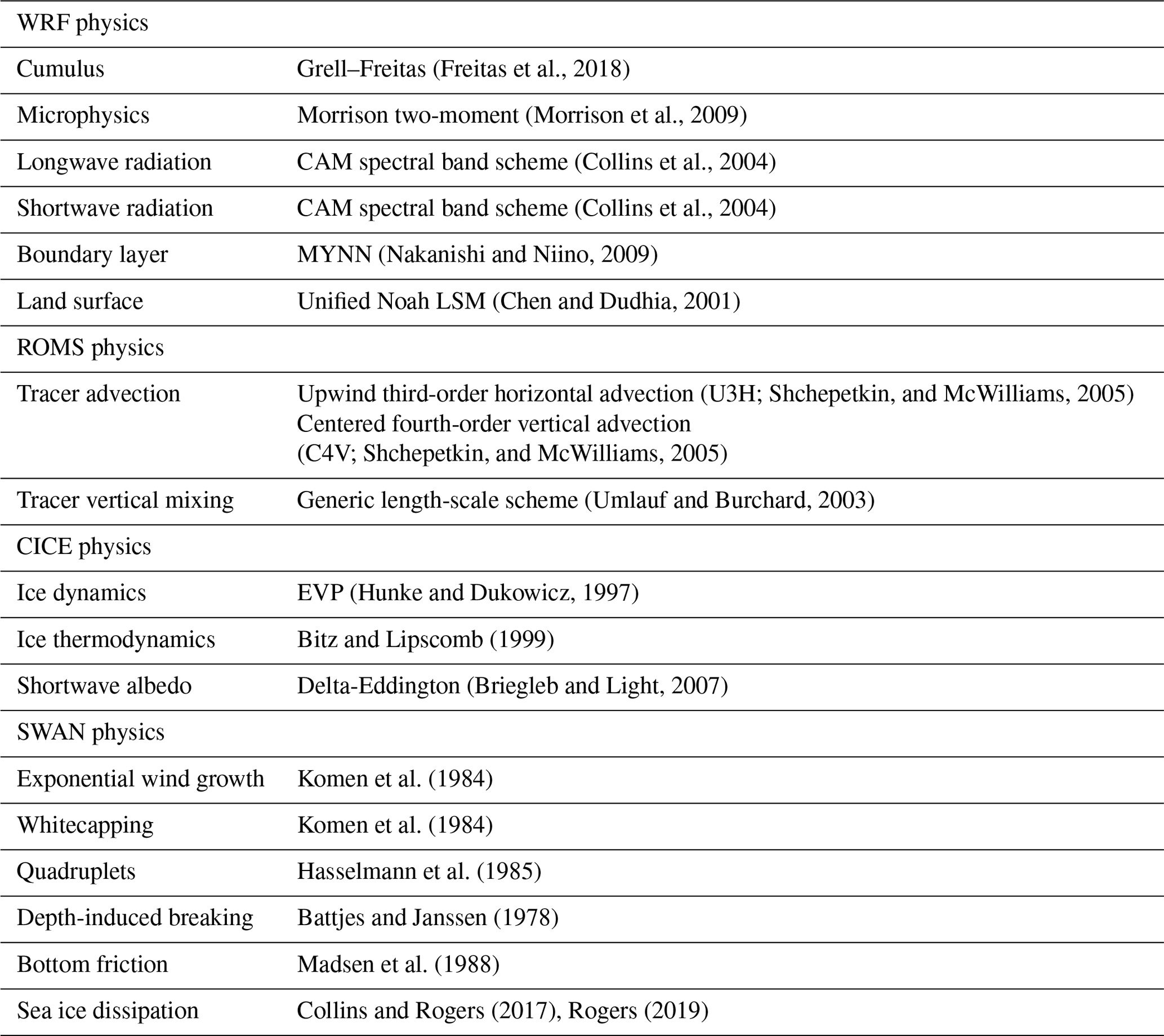
The WRF, ROMS, SWAN, and CICE models use the same model grid with 320 (440) x (y) grid points and ∼ 24 km horizontal resolution (Fig. 1). Initial and boundary conditions for the WRF, ROMS, and CICE models are generated from the Climate Forecast System Version 2 (CFSv2; Saha et al., 2014) operational analysis, archived by the National Centers for Environmental Information (NCEI), the National Oceanic and Atmospheric Administration (DOC/NOAA/NWS/NCEP, https://www.ncei.noaa.gov/access/metadata/landing-page/bin/iso?id=gov.noaa.ncdc:C00878, last access: 20 May, 2023). In our configurations, the SWAN model starts with the calm wave states (i.e., zero wave energy at all frequencies). The modified FSTD, L(r,h), is initialized based on the power-law distribution of floe number, (e.g., Toyota et al., 2006), with the exponent a as 2.1 for all grid cells. Physical parameterizations of each model component are mostly identical to those used in Yang et al. (2022) and are summarized in Table 1.
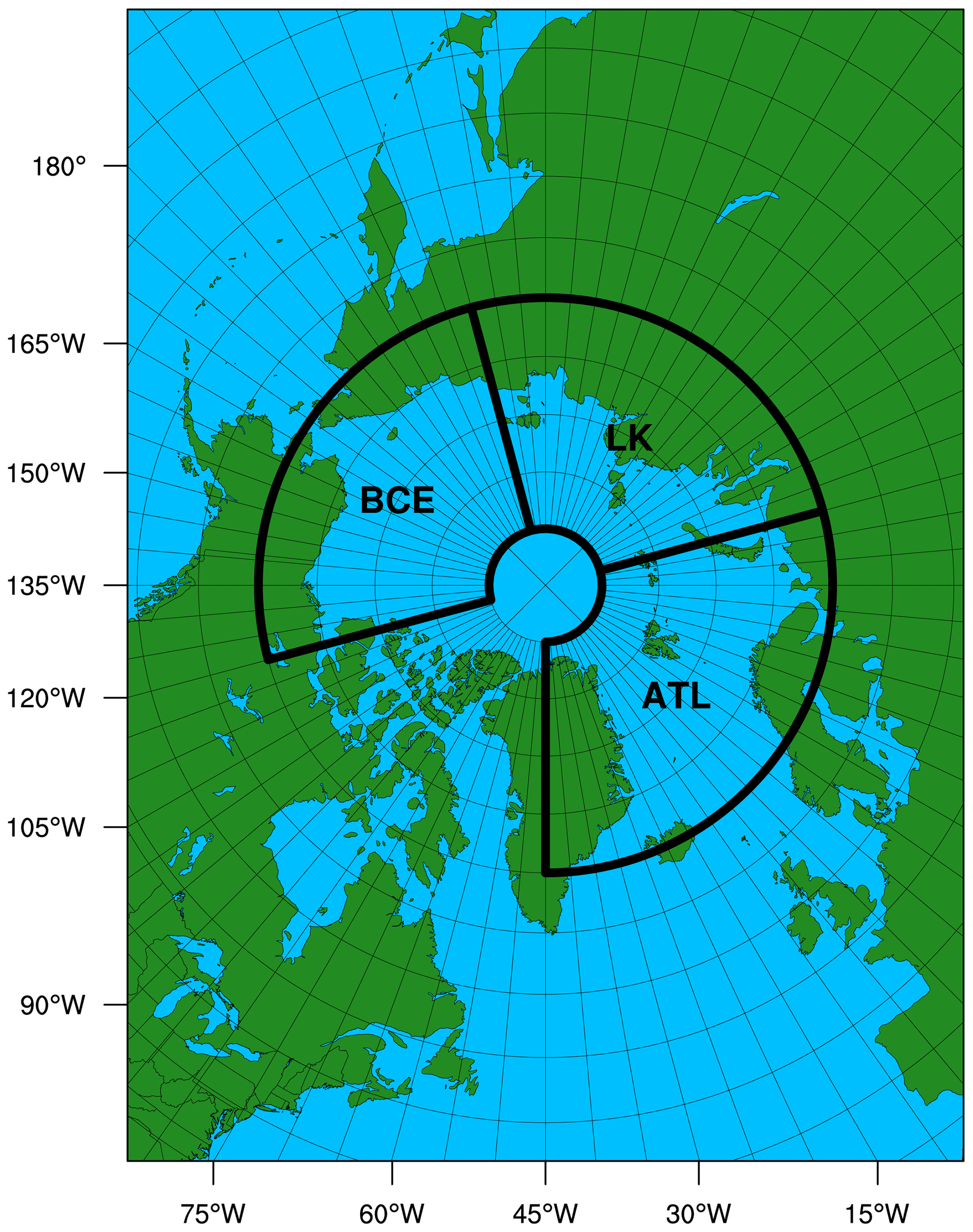
Figure 1The model domain used in CAPS for pan-Arctic sea ice simulations. Black boxes indicate the subregions for analysis performed in this study.
Table 1The summary of physics parameterizations used in all pan-Arctic simulations.
Cassano et al. (2011) suggested that the use of a higher model top (10 mb) or applying spectral nudging in the upper model levels leads to significantly reduced bases in pan-Arctic atmospheric circulation in the standalone WRF model. Thus, compared with Yang et al. (2022), we change the model top of the WRF model in CAPS from 50 to 10 mb. With coupling to the SWAN model in CAPS, the corresponding configurations are modified to reflect wave effects on the atmosphere and the ocean. In the Mellor–Yamada–Nakanishi–Niino planetary boundary layer scheme (MYNN; Nakanishi and Niino, 2009), the surface roughness, z0, is modified to include the effect of waves based on the following formulation:
where υ is the viscosity and u∗ is the friction velocity (Taylor and Yelland, 2001; Warner et al., 2010). For the interaction of ocean waves and currents, the vortex-force (VF) formulation is applied that represents conservative (e.g., vortex and Stokes–Coriolis forces) and non-conservative wave effects. The non-conservative wave effects in the VF formulation include wave accelerations for currents and wave-enhanced vertical mixing (Kumar et al., 2012; Uchiyama et al., 2010). The dissipated wave energy due to surface wave breaking and whitecapping is transferred to the ocean surface layer as additional turbulent kinetic energy, which in turn enhances the vertical mixing. For the effect of currents on the dispersion relation in wave propagation, we employ a depth-weighted current to account for the vertically sheared flow following Kirby and Chen (1989). As discussed in previous studies (e.g., Naughten et al., 2017; Yang et al., 2022), the upwind third-order advection (U3H, Table 1) scheme, which is an oscillatory scheme, can lead to increased non-physical frazil ice formation. To address this issue, we implement the upwind flux limiter suggested by Leonard and Mokhtari (1990) to reduce false extrema caused by the oscillatory behavior of the U3H scheme. The value of yielding strain εc, described in Sect. 2.3.1, Eq. (15), is chosen as (Dumont et al., 2011; Horvat and Tziperman, 2015; Langhorne et al., 1998). The floe-welding parameter in the thermodynamic term ℒT is chosen as km−2 s−1. Roach et al. (2018b) found a lower bound of the floe-welding parameter as km−2 s−1 in the autumn Arctic based on the observations. Also, the floe-welding process only occurs in the freezing condition (Roach et al., 2018a), and the freezing condition is determined by net ice mass increase by thermal mass change (see Fig. 3). The floe-welding parameter will behave like a step function during the freeze–thaw transition. For the user-defined coefficients in Eq. (4), all experiments use the equally redistributed formulation described in Sect. 2.3.1 with cw as 0.8 and ∝ as 1.0. Based on the formation of ℒT in Eq. (9) (see Roach et al., 2018a), the floe size change through the lateral surface is determined by both the floe size and the lateral melting rate. In the existing sea ice models, the lateral melting rate wlat is based on the empirical formulation suggested by Perovich (1983, hereafter P83):
where ΔT is the temperature difference between sea surface temperature (SST) and the freezing point, and m1 and m2 are empirical coefficients based on the observations from a single sea ice lead in the Canadian Arctic. This empirical formulation is also the default lateral melting rate in the CICE model. Maykut and Perovich (1987, hereafter MP87) showed a different approach to parameterizing the lateral melting rate that includes the friction velocity u∗ based on the observations from the Marginal Ice Zone Experiment, and it is defined as
Both formulations (Eqs. 23, 24) are examined in this study (see Table 2). In Eq. (2), the user-defined coefficients for the wave attenuation are set as and (case 1), which follow the polynomial of Meylan et al. (2014, hereafter M14) from the observations with 10–25 m floe in diameter in the Antarctic, and and (case 2), which follow the polynomial of Rogers et al. (2018, hereafter R18) based on the observations for pancake and frazil ice in the Arctic.
Table 2A summary of the experiments conducted in this study and their main changes in the experiment design. MP87: Maykut and Perovich (1987). P83: Perovich (1983). M14: Meylan et al. (2014). R18: Rogers et al. (2018).
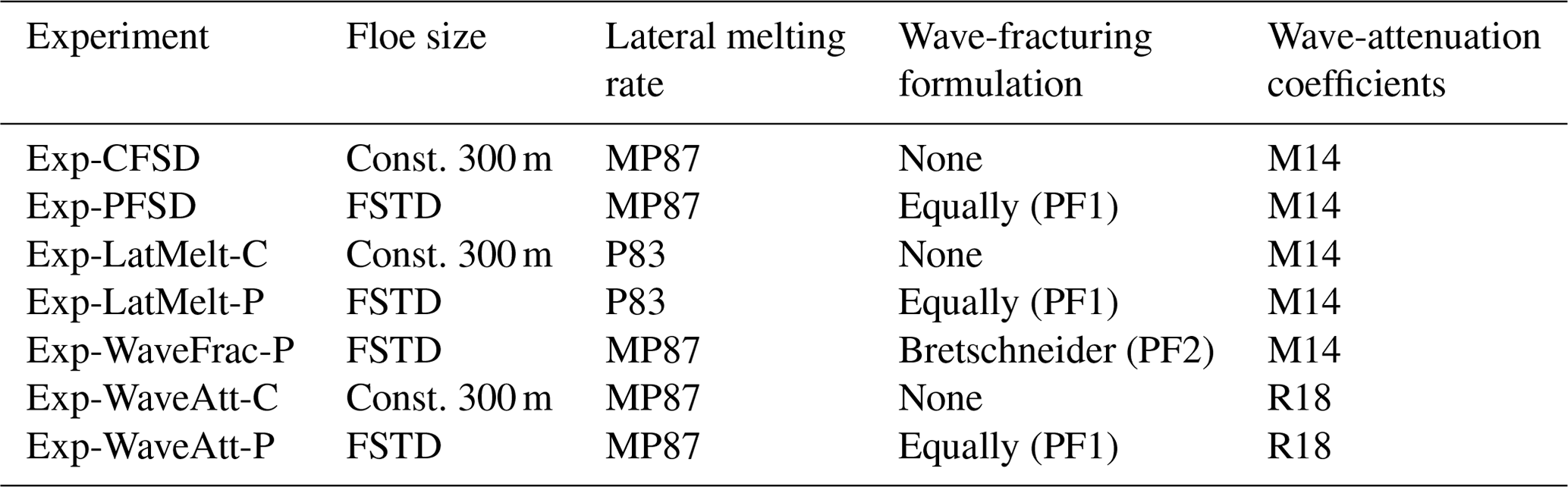
In this study, a series of numerical experiments for the pan-Arctic sea ice simulation have been conducted, from 1 January 2016 to 31 December 2020. Table 2 provides the details of the configurations for these experiments, which allow us to examine the influence of ocean waves and related physical processes on Arctic sea ice simulation in the atmosphere–ocean–wave–sea ice coupled framework. Specifically, these experiments focus on (1) the comparison between constant FSD and prognostic FSD (Exp-CFSD and Exp-PFSD), (2) sea ice responses to different lateral melting rate parameterizations (Exp-CFSD, Exp-PFSD, Exp-LatMelt-C, and Exp-LatMelt-P), (3) the difference between the equally redistributed formulation and the Bretschneider formulation for floe fracturing (Exp-PFSD and Exp-WaveFrac-P), and (4) the contribution of different wave attenuation rates to sea ice changes (Exp-CFSD, Exp-PFSD, Exp-WaveAtt-C, and Exp-WaveAtt-P).
4.1 Constant vs. prognostic floe size
Figure 2 shows the evolution of sea ice area (SIA) for all experiments conducted in this study (the values of seasonal maximum and minimum SIA for all experiments are summarized in Table S1). SIA is calculated as the sum of the ice-covered area of all grid cells (cell area times sea ice concentration). In addition to the evolution of SIA, the 2016–2020-averaged March and September sea ice concentration (SIC) for all experiments is shown in Fig. S1. Compared with Exp-CFSD, which uses a constant floe diameter (300 m) in the lateral melting scheme (Steele, 1992), Exp-PFSD uses the equations described in Sect. 2.2 to determine the prognostic FSD and related physical processes (see Table 2). With the prognostic FSD, the evolution of SIA in Exp-PFSD (Fig. 2a, red line) shows smaller SIA in the melting months (June to September) and a similar magnitude of SIA in other months compared to that of Exp-CFSD (Fig. 2a, blue line) during 2016–2018. After that, Exp-PFSD simulates smaller SIA than that of Exp-CFSD for most months during 2019–2020, especially for the seasonal maximum of 2019 and SIA after May 2020.
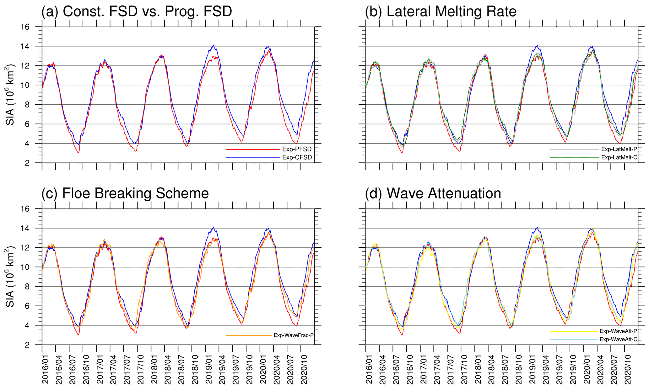
Figure 2Time series of Arctic sea ice area for Exp-CFSD (blue line), Exp-PFSD (red line), Exp-LatMelt-C (green line), Exp-LatMelt-P (grey line), Exp-WaveFrac-P (orange line), Exp-WaveAtt-C (light-blue line), and Exp-WaveAtt-P (yellow line). The date format is year/month.
Figure 3 shows the evolution of sea ice mass budget terms with cell-area-weighted averaging over the entire model domain with a 15 d running average for smoothing out high-frequency fluctuations for all experiments. The most notable difference between Exp-CFSD and Exp-PFSD is the magnitude of basal melt (red lines) and lateral melt (grey lines). In Exp-CFSD, basal melt plays the dominant role in reducing sea ice mass compared to lateral melt, which makes a negligible contribution to the total mass change. As discussed in Maykut and Perovich (1987), the inclusion of friction velocity in calculating the lateral melting rate results in wlat→0 as , which contributes to negligible lateral melt in Exp-CFSD. By contrast, Exp-PFSD with prognostic floe size shows that lateral melt makes the major contribution in reducing ice mass (Fig. 3b), a result of smaller floe size near the ice edge simulated by Exp-PFSD (Fig. 10a). It is also notable that the increased lateral melt in Exp-PFSD tends to be compensated for by the decreased basal melt (Fig. 3b). The overall ice melt due to oceanic processes in Exp-PFSD (i.e., the sum of lateral melt and basal melt) does not change significantly compared to that of Exp-CFSD (Fig. S2e). The melting potential in the CICE model of CAPS, the available energy from the ocean to melt sea ice, is defined as the vertical integral of the difference between the ocean temperature and freezing point within the surface layer (to 5 m depth in CAPS) from the ROMS model. When the available oceanic energy is less than the sum of heat fluxes used for lateral and basal melt, the CICE model performs a linear scaling to maintain the relative magnitude of heat fluxes for lateral and basal melt. Thus, the increased energy consumption by lateral melt due to smaller floe size reduces the available energy for basal melt. Such a change between lateral and basal melt has been shown in some studies (e.g., Bateson et al., 2020, 2022; Roach et al., 2018a, 2019; Smith et al., 2022; Tsamados et al., 2015). Although it is a rough compensation, Exp-PFSD simulates more ice melted by the oceanic energy compared to Exp-CFSD from January to July (Fig. S2e).
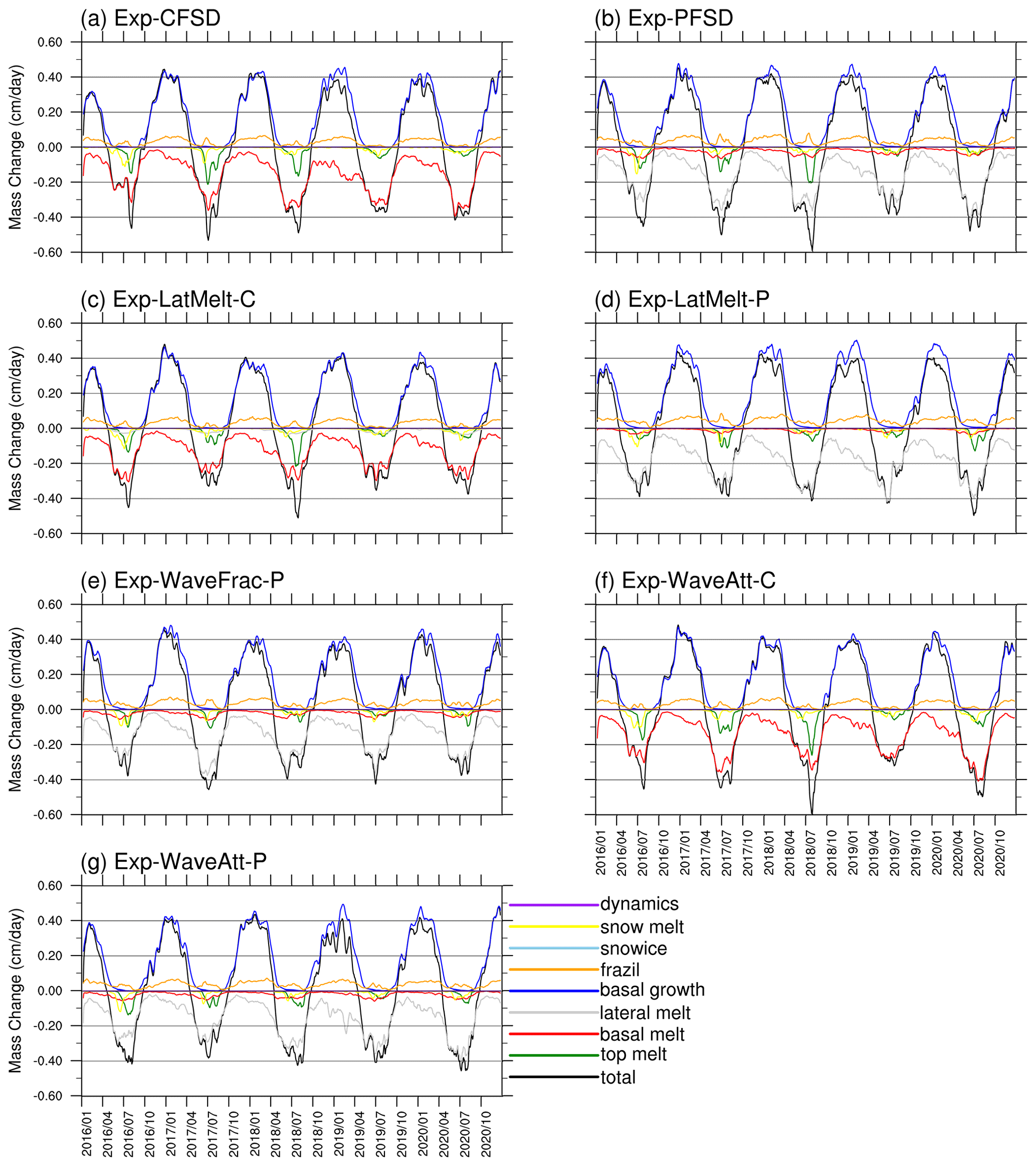
Figure 3Time series (15 d running average) of sea ice mass budget terms for (a) Exp-CFSD, (b) Exp-PFSD, (c) Exp-LatMelt-C, (d) Exp-LatMelt-P, (e) Exp-WaveFrac-P, (f) Exp-WaveAtt-C, and (g) Exp-WaveAtt-P. Ice mass budget terms include total mass change (black line), sea ice melt at the air–ice interface (top melt, green line), sea ice melt at the bottom of the ice (basal melt, red line), sea ice melt at the sides of the ice (lateral melt, grey line), sea ice growth at the bottom of the ice (basal growth, blue line), sea ice growth by supercooled open water (frazil, orange line), sea ice growth due to transformation of snow to sea ice (snowice, light-blue line), and sea ice mass change due to dynamics-related processes (dynamics, purple line) (Notz et al., 2016; Yang et al., 2022). For reference, the snowmelt term (yellow line) is included. The date format is year/month.
Figure 4 shows the evolution of ice–ocean heat flux, the friction velocity at the ice–ocean interface, and the temperature difference between SST and the freezing point for Exp-CFSD and Exp-PFSD. These variables are the average of ice-covered cells with at least 1 % ice concentration, and the ice–ocean heat flux is weighted by the ice concentration so that the weighted heat flux represents the mean value of the cell, rather than the mean value of the ice–ocean interface. It should be noted that cells with negative values of the temperature difference (i.e., supercooled water) are forced to be zero. This is consistent with the treatment in the CICE model for the calculation of ice–ocean heat flux. As shown in Figs. 4a and S2e, the evolution of ocean-induced ice melt is consistent with that of the ice–ocean heat flux for both Exp-CFSD and Exp-PFSD. Both Exp-CFSD and Exp-PFSD show relatively similar evolution of the friction velocity (Fig. 4b). The temperature difference of Exp-PFSD is much smaller than that of Exp-CFSD (Fig. 4c). The ice–ocean heat flux is the total heat flux from ocean to ice through the ice bottom surface and lateral surface. Although Exp-PFSD has a smaller temperature difference as well as the melting potential under ice-covered cells, the larger total ice surface area due to smaller floe size increases the efficiency of Exp-PFSD extracting energy from the ocean. The smaller temperature difference of Exp-PFSD and the compensation between lateral and basal melt suggest that the ocean surface layer of Exp-PFSD is closer to the freezing point compared to that of Exp-CFSD. Energy loss from the ocean through air–sea heat flux in winters, which further cools the upper ocean; freshwater input (e.g., ice melting, precipitation) that raises the freezing point; and non-physical numerical oscillations (Naughten et al., 2017; Yang et al., 2022) are potential contributors that lead to increased frazil ice formation of Exp-PFSD as shown in Figs. 3a–b and S2g.
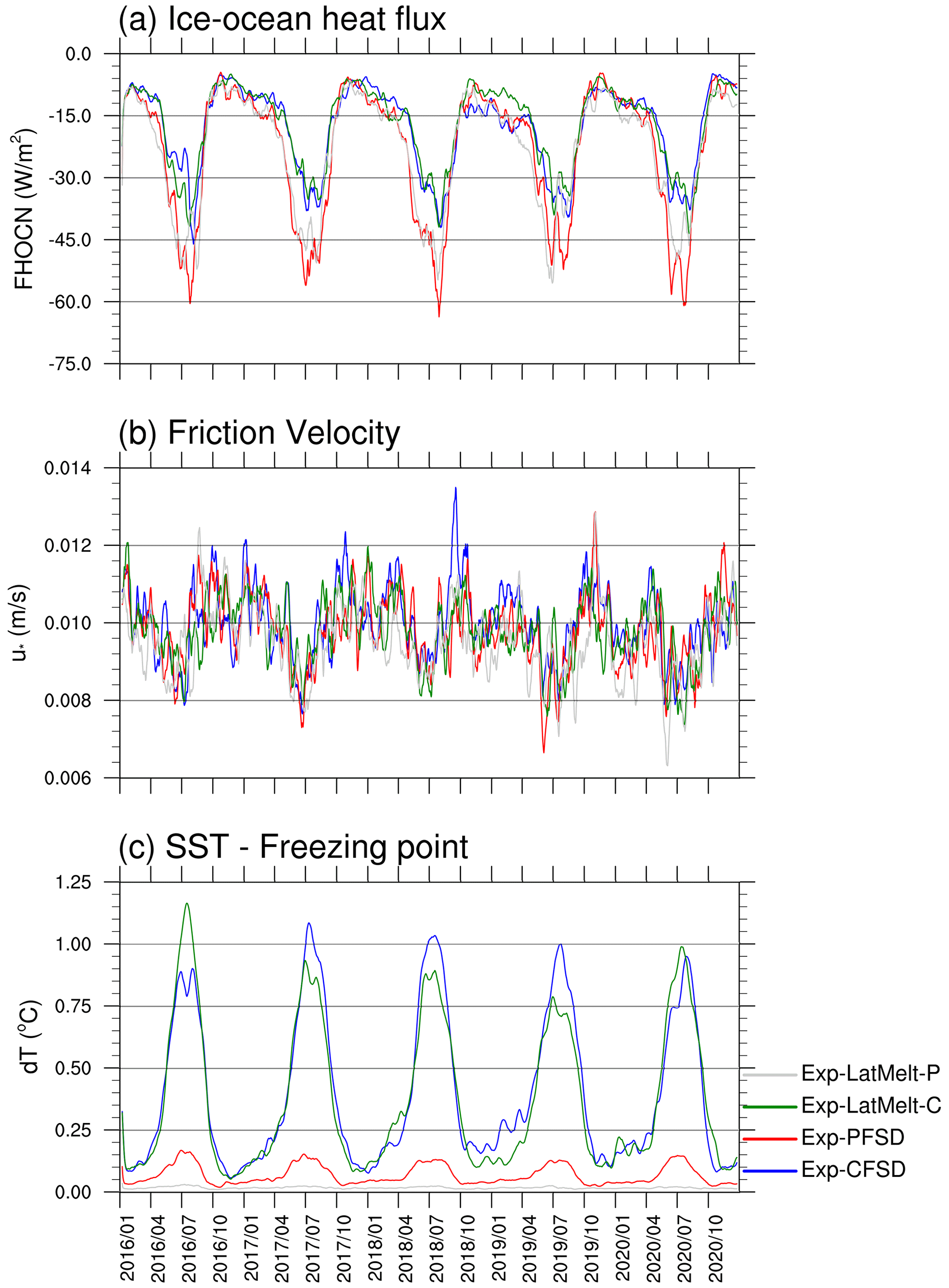
Figure 4Time series (15 d running average) of (a) ice–ocean heat flux, (b) friction velocity at the ice–ocean interface, and (c) the temperature difference between SST and the freezing point for Exp-CFSD (blue line), Exp-PFSD (red line), Exp-LatMelt-C (green line), and Exp-LatMelt-P (grey line). Note that (a) is positive downwards and weighted by ice concentration. The date format is year/month.
Figure 5 shows the heat flux budget at the ice surface averaged for all ice-covered cells. The positive ice–atmosphere heat fluxes of Exp-CFSD and Exp-PFSD in July (Fig. S3a) correspond to top melt in Figs. 3a–b and S2b (as well as Table S2). The ice–atmosphere heat flux determines not only the magnitude of ice surface melt in summer but also the energy loss from the ice interior in winter, which is crucial for ice growth. As shown in Fig. S3a, Exp-PFSD loses more energy to the atmosphere than Exp-CFSD in most winters. The conductive heat flux also shows similar evolution, suggesting that more energy is conducted to the ice top from ice layers below in Exp-PFSD (Fig. S3b). The loss of ice energy then contributes to increased ice growth at the ice bottom as shown in Figs. 3a–b and S2f (as well as Table S2). Generally, the net shortwave flux of Exp-PFSD is larger (ice gains more energy) than that of Exp-CFSD, especially during the melting season (Fig. S3c). In contrast to the net shortwave flux, for most of the time, the net longwave flux of Exp-PFSD is smaller (i.e., ice loses more energy) than that of Exp-CFSD (Fig. S3d). Exp-PFSD loses more energy through sensible heat flux compared to Exp-CFSD (Fig. S3e). For latent heat flux, there are no common features between Exp-PFSD and Exp-CFSD, suggesting a difference in the simulation of atmospheric transient systems (Fig. S3f).
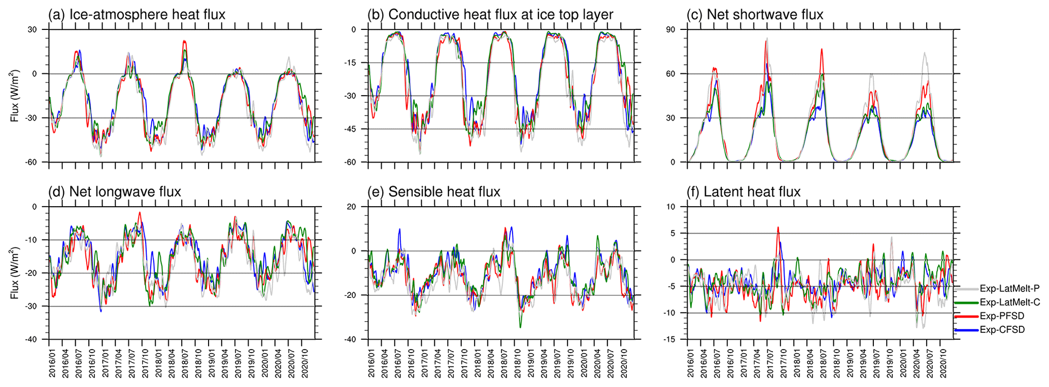
Figure 5Time series (15 d running average) of (a) ice–atmosphere heat flux, (b) conductive heat flux at the ice top layer, (c) net shortwave flux, (d) net longwave flux, (e) sensible heat flux, and (f) latent heat flux for Exp-CFSD (blue line), Exp-PFSD (red line), Exp-LatMelt-C (green line), and Exp-LatMelt-P (grey line). Note that (a)–(e) are positive downwards and weighted by ice concentration. The date format is year/month.
The ice mass budget in Fig. 3 is not directly related to the evolution of SIA in Fig. 2, since each process acts differently in changing SIA. For vertical processes (i.e., top melt, basal melt), ice must be vertically melted completely to reduce SIA. Lateral melt, on the contrary, can directly reduce SIA (Smith et al., 2022). Figure 6 shows the evolution of SIA changes due to thermal processes (top melt, basal melt, lateral melt, frazil ice formation) and dynamical processes (transport, ridging). For thermal-area changes, Exp-PFSD (red line), in general, shows comparable ice area changes to those of Exp-CFSD (blue line) for most of the period (Fig. 6a). Compared with Fig. S2g, the timings of when Exp-PFSD shows more thermally increased ice area correspond to increased frazil ice formation, which primarily occurs in open water. In contrast to thermal-area changes, dynamical-area changes of Exp-PFSD tend to reduce ice area relative to that of Exp-CFSD (Fig. 6e). Dynamically induced area changes are partly due to the ridging scheme (Lipscomb et al., 2007) that favors the conversion of thin ice to thicker ice and reduces total ice area but preserves the total volume. In general, Exp-PFSD has a higher fraction of ice in the thinner ITD range than Exp-CFSD.
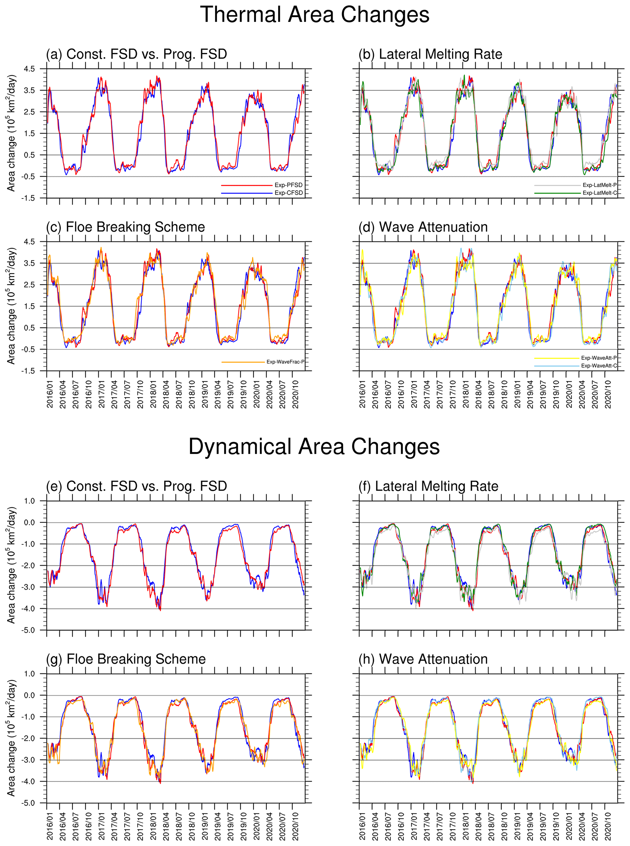
Figure 6Time series (15 d running average) of sea ice area changes due to thermal processes (a–d, upper panels) and dynamical processes (e–h, bottom panels) for Exp-CFSD (blue line), Exp-PFSD (red line), Exp-LatMelt-C (green line), Exp-LatMelt-P (grey line), Exp-WaveFrac-P (orange line), Exp-WaveAtt-C (light-blue line), and Exp-WaveAtt-P (yellow line). The date format is year/month.
Based on geographic features, we define the following subregions for further analysis: the (1) Barents and Greenland seas (ATL; 65–85° N, 45° W–60° E); (2) Laptev and Kara seas (LK; 65–85° N, 60–150° E); and (3) Beaufort, Chukchi, and East Siberian seas (BCE; 65–85° N, 150° E–120° W; see black boxes in Fig. 1 for the geographic coverage of subregions). The fetches of the ATL, LK, and BCE regions are limited by the surrounding continents and the seasonal evolution of ice-covered areas. The ATL region is only partially limited by ice-covered areas, while the LK and BCE regions can be fully covered by sea ice in winter. Though these subregions also include part of the central Arctic Ocean, they will still be addressed as the main peripheral seas in the subregions in the following discussion for simplicity. Figure 7 shows the evolution of the sea ice extent, sea ice area, domain-averaged significant wave height, melting potential, and heat flux at the ocean surface (FLUXOCN, including ice–ocean and atmosphere–ocean interfaces) of Exp-CFSD and Exp-PFSD. As shown in Fig. 7a–i, it is clear that the higher (lower) significant wave height corresponds to less (more) regional ice coverage for all subregions. For the melting potential (Fig. 7j–l), the difference between Exp-CFSD (blue line) and Exp-PFSD (red line) in August, in general, is correlated with FLUXOCN in July (Fig. 7m–o). The higher (lower) incoming heat flux to the ocean due to less (more) ice-covered area increases (decreases) energy stored in the ocean surface layer. However, FLUXOCN alone cannot explain the difference in the melting potential for the entire period. For example, Exp-PFSD shows more melting potential after December 2019 in the ATL region (Fig. 7j) and more melting potential in December 2017 in the LK region (Fig. 7k) compared to Exp-CFSD. These timings do not show corresponding FLUXOCN values in the preceding month, suggesting the contribution of different processes. Figure 8 shows the evolution of wave energy dissipation due to whitecapping and the difference in the temperature profile in the upper 150 m for Exp-CFSD and Exp-PFSD. As described in Sect. 3, wave energy dissipation increases the turbulent kinetic energy in the surface layer and thus vertical mixing. Dissipation due to surface wave breaking is zero for most of the period. Occasionally, there are non-zero dissipations due to surface wave breaking for Exp-CFSD and Exp-PFSD. The evolution of wave dissipation due to whitecapping (Fig. 8a–c) is in good agreement with that of the significant wave height in Fig. 7g–i. This suggests that stronger-wave conditions associated with less ice-covered areas increasing the effect of vertical mixing. Combined with the warmer upper ocean in Exp-PFSD after January 2020 in the ATL region and in December 2017 in the LK region in Fig. 8d–e, the strengthened vertical mixing brings warmer water of the subsurface upwards and maintains/increases the melting potential in the subregions. Figure 8d–f also show that the warmer signal in the upper ocean (at least to 60 m depth) of Exp-PFSD persists after July 2018 in the ATL region while the LK and BCE regions show seasonal oscillation of ocean temperature in the upper ocean for the entire simulation. Combined with the regional SIA shown in Fig. 7d–f, seasonal fully ice-covered states in the LK and BCE regions force the upper ocean to be restored to certain states (i.e., near-freezing point under sea ice, near-zero melting potential shown in Fig. 7k–l) for both Exp-CFSD and Exp-PFSD, which might mitigate the effects of ocean wave activities and other processes on the upper ocean. With a less restorative effect by sea ice on the upper ocean in the ATL region, the difference in the thermally induced mass change between Exp-PFSD and Exp-CFSD shows a larger variation once the upper ocean difference starts to persist after July 2018 (Figs. 8d, S4d), while the variations in the LK and BCE regions remain relatively unchanged for the entire simulation (Fig. S4e–f).
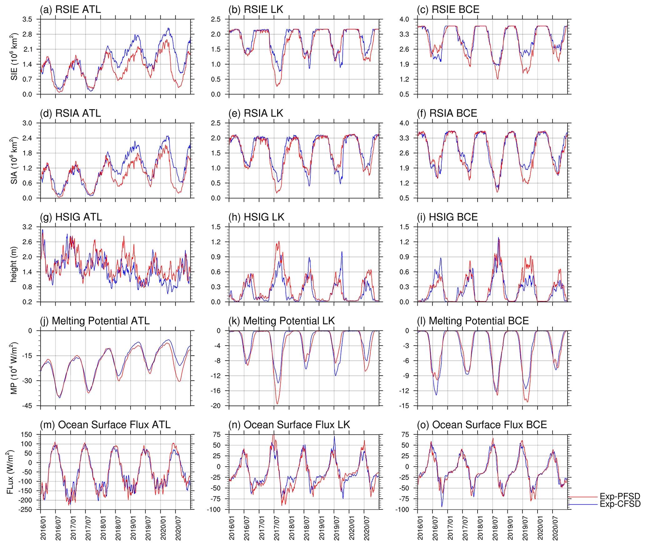
Figure 7Time series of (a–c) ice extent, (d–f) ice area, (g–i) significant wave height, (j–l) melting potential, and (m–o) heat flux at the ocean surface in the ATL, LK, and BCE regions for Exp-CFSD (blue line) and Exp-PFSD (red line). Note that significant wave height, melting potential, and heat flux at the ocean surface are region-averaged and 15 d running-average values. The date format is year/month.
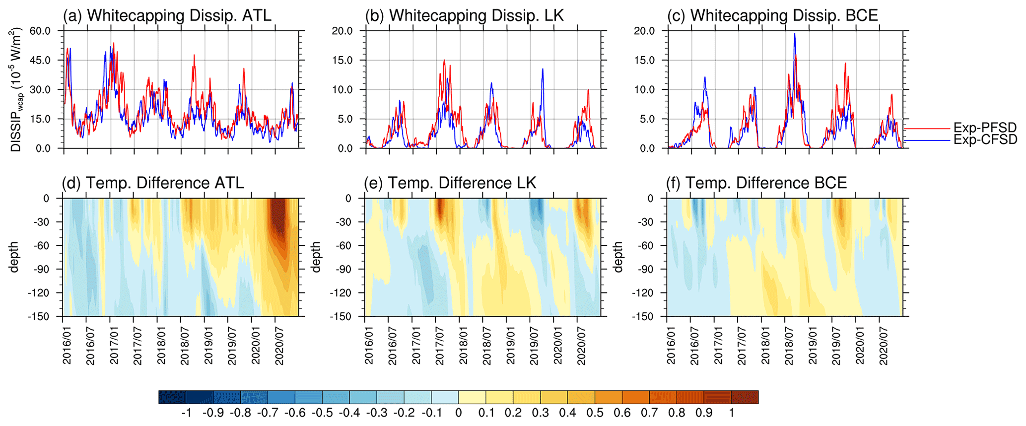
Figure 8Time series (15 d running average) of whitecapping dissipation averaged over the (a) ATL, (b) LK, and (c) BCE regions for Exp-CFSD (blue line) and Exp-PFSD (red line) and the temperature profile difference between Exp-CFSD and Exp-PFSD in the upper 150 m averaged over (d) ATL, (e) LK, and (f) BCE regions. The date format is year/month.
Additionally, atmospheric circulation responds to the changes in the spatial distribution of sea ice (Fig. S1). As shown in Fig. S5, Exp-PFSD tends to have anomalous anti-cyclonic circulations in September compared to Exp-CFSD, but there is no consistent center of action during the entire period. In March, Exp-PFSD tends to simulate anomalous cyclonic circulations in the Barents–Kara seas for most of the years compared to Exp-CFSD, except in 2019. The responses in the atmospheric state in both experiments also influence sea ice movement, which further contributes to the regional ice differences in Fig. 7a–f, as well as the heat flux budgets in Fig. S3.
4.2 Sensitivity to lateral melting rate parameterization
In addition to the floe size as discussed in the above section, the lateral melting rate (wlat) is an important factor contributing to the relative strength of lateral and basal melt. As described in Sect. 3, we conduct the experiments with the lateral melting rate suggested by Perovich (1983, P83) and Maykut and Perovich (1987, MP87) (see Table 2) to examine the sensitivity of Arctic sea ice simulation to different lateral melting rate parameterizations. As shown in Fig. 2b, the simulated summer sea ice areas of Exp-LatMelt-C (green line) and Exp-LatMelt-P (grey line), in general, are larger than those of Exp-CFSD (blue line) and Exp-PFSD (red line).
As shown in the sea ice mass budget (Fig. 3a, c), Exp-LatMelt-C, which does not include the friction velocity in the formulation (Eq. 23) but keeps other model configurations the same as Exp-CFSD, only shows a slightly larger contribution to lateral melt during summer months (Fig. S6d). Also, the contribution to basal melt by Exp-LatMelt-C is generally smaller than that in Exp-CFSD (Fig. S6c). Similarly to the experiments with the MP87 scheme, Exp-LatMelt-P with the prognostic FSD also shows the compensation between lateral melt and basal melt compared to Exp-LatMelt-C (Fig. 3c, d). Exp-LatMelt-P shows stronger lateral melt compared to Exp-PFSD, which is contributed by the P83 formulation (Fig. S6d). Despite the stronger lateral melt in Exp-LatMelt-P, its basal melt is smaller compared to Exp-PFSD (Fig. S6c). Thus, the ocean-induced melt of Exp-LatMelt-P is broadly similar to that of Exp-PFSD. The result of Exp-LatMelt-P and Exp-PFSD suggests that the changes in lateral and basal melt due to different lateral melting rate parameterizations are mostly controlled by the available energy from the ocean (i.e., melting potential).
Exp-LatMelt-P simulates more basal growth in winter (Fig. S6f), which is contributed by more energy loss to the atmosphere (Fig. 5a), in comparison to Exp-PFSD. Also, more frazil ice formation is simulated in Exp-LatMelt-P than Exp-PFSD during most of the simulation period (Fig. S6g). The combined effects of the above processes lead to Exp-LatMelt-P showing less total ice melt in summer and similar ice growth in winter compared to Exp-PFSD (Fig. S6a). Due to more frazil ice formation, Exp-LatMelt-P shows more thermally increased ice area compared to Exp-PFSD (Figs. 6, S6g). Frazil ice formation reduces open-water areas and blocks the energy exchange between the atmosphere and the ocean. That is, the upper ocean under sea ice in Exp-LatMelt-P receives less incoming flux from the atmosphere (i.e., solar radiation) during April to September (not shown) to balance the energy consumption by ice melt, which leads to a smaller ocean temperature difference compared to Exp-PFSD (Fig. 4c, green and red lines).
Figure 9 shows the spatial distribution of sea ice concentration, sea surface temperature, and friction velocity in September 2020 for the experiments using the MP87 and P83 schemes. Exp-CFSD, Exp-PFSD, and Exp-LatMelt-C simulate large areas with ice concentration less than 5 % (they are mostly much less than 1 %; Fig. 9a–c). Opposite to these three experiments, Exp-LatMelt-P does not show wide areas with non-zero and infinitesimal ice concentration (Fig. 9d). Although these areas only account for a tiny fraction of total sea ice, they may still be a source of uncertainty for sea ice simulations. Cells with ice present can be influenced by all processes involved in the sea ice mass budget (Fig. 3), while ice-free cells can only be affected by frazil ice formation and dynamical advection. Under these small-ice areas, SST is well above the freezing point (Fig. 9e–h) and the friction velocity is mostly less than m s−1 (Fig. 9i–l). In our configuration of the CICE model, the minimum value of friction velocity is set to m s−1. This suggests that the friction velocity is the limiting factor for heat flux transferred into sea ice in the small-ice areas. For basal heat flux, the formulation in the CICE model is based on Maykut and McPhee (1995), which is controlled by the friction velocity and the temperature difference. Thus, basal heat fluxes with small friction velocities may not be large enough to satisfy the energy convergence (in conjunction with conductive heat flux at the ice bottom) at the ice–ocean interface to melt ice if the temperature difference does not show a larger magnitude. Since the MP87 scheme includes the friction velocity, lateral heat flux is also limited in small-ice areas. Exp-PFSD has a much smaller floe size (compared to 300 m) in these small-ice areas, but the increased strength of lateral melt does not overcome the limitation of friction velocity to melt ice completely (Fig. 9b). The P83 scheme, which does not include the friction velocity, is controlled by the temperature difference, but the effect of lateral melting in Exp-LatMelt-C is largely constrained by a constant 300 m floe diameter. Liang et al. (2019) suggested these small-ice areas can be eliminated by assimilating SST observations. The results of Exp-LatMelt-P suggest a model physics approach that considers the prognostic FSD and the lateral melting rate to reduce the coverage of small-ice areas near the ice edge.
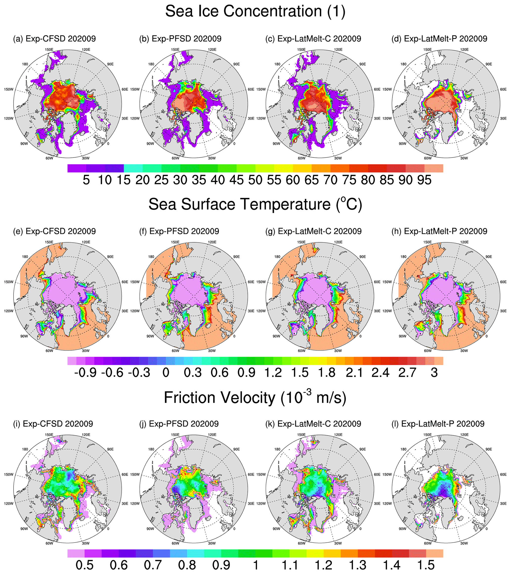
Figure 9The monthly mean of (a–d) sea ice concentration, (e–h) sea surface temperature, and (i–l) friction velocity in September 2020 for Exp-CFSD, Exp-PFSD, Exp-LatMelt-C, and Exp-LatMelt-P. The date format is yyyymm (year followed by month).
4.3 Sensitivity to floe-fracturing parameterization
The equally redistributed formulation (hereafter PF1) for floe fracturing described in Sect. 2.3.1 does not have a preferential floe size after fracturing (i.e., a stochastic process). However, the size of fractured floes can be predicted based on the properties of surface ocean waves, particularly the wavelength (Dumont et al., 2011; Horvat and Tziperman, 2015). In this section, we conduct an experiment (Exp-WaveFrac-P; see Table 2) that utilizes a semi-empirical wave spectrum to redistribute fractured floes (see Sect. 2.3.2 for details; hereafter PF2) to explore the effects of different wave-fracturing formulations on Arctic sea ice simulation. As shown in Fig. 2c, Exp-WaveFrac-P (orange line) simulates larger SIA in summer and similar SIA in winter compared to that of Exp-PFSD (red line).
By applying different formulations for floe fracturing (as well as different lateral melting rate formulations), FSD responds accordingly. To quantify the responses of FSD associated with different physical configurations (Table 2), the representative floe radius ra, as well as its tendency due to different processes in Eq. (9), is utilized and calculated as (Roach et al., 2018a)
Figure 10 shows the spatial distribution of the representative floe radius in winter and summer for all experiments with the prognostic FSD. As described in Sect. 3, L(r,h) is initialized by the power-law distribution with the exponent as 2.1 for all experiments. Exp-WaveFrac-P shows a smaller floe radius in the Chukchi and East Siberian seas and north of Greenland at the early stage of simulation compared to experiments using the PF1 formulation (Fig. 10a–o, upper panel). Small-floe areas in Exp-WaveFrac-P are mostly contributed by the effect of wave fracturing where a decreasing tendency of floe radius can extend further into the central Arctic from the Atlantic and the Bering Strait compared to PF1 experiments (Fig. S7). After September 2016, the representative floe radii of PF experiments emerge; that is, Exp-WaveFrac-P has a smaller floe size compared to PF1 experiments for both winter and summer (Fig. 10a–o). In summer, Exp-WaveFrac-P shows mostly fully fractured floes (<10 m, Fig. 10k–o, bottom panel). The stronger wave fracturing shown in Exp-WaveFrac-P is partly contributed by the semi-empirical wave spectrum used in PF2. The simulated wave parameters under the ice-covered area are mostly with Hs<0.01 m s−1 and Tp>15 s. The constructed wave spectrum and amplitude based on simulated wave parameters under sea ice and Eqs. (17) and (18) still include the contribution from high-frequency waves (T=2 s bin), especially in the ice pack far from the ice edge. The high-frequency waves only account for a small fraction in the wave period distribution and have a small wave amplitude A(T) (). The strain of the high-frequency bin based on Eq. (20) still exceeds the yielding strain and then fractures ice floe into the smallest floe size category. Observational and numerical studies showed that high-frequency waves rapidly decay and reach the “zero” transmission state for high-frequency waves when traveling under sea ice (e.g., Collins et al., 2015; Liu et al., 2020). Despite the over-fracturing behavior shown in Exp-WaveFrac-P, the prevalence of small floes does not translate into stronger ocean-induced ice melt but weaker melt in summer compared to Exp-PFSD (Figs. 3d–e, S8e), indicating the limiting role of melting potential. The weaker ocean-induced ice melt in the summer of Exp-WaveFrac-P corresponds to smaller ice–ocean heat fluxes (Fig. S9a), which is contributed by both smaller friction velocity and smaller temperature difference (Fig. S9b–c).
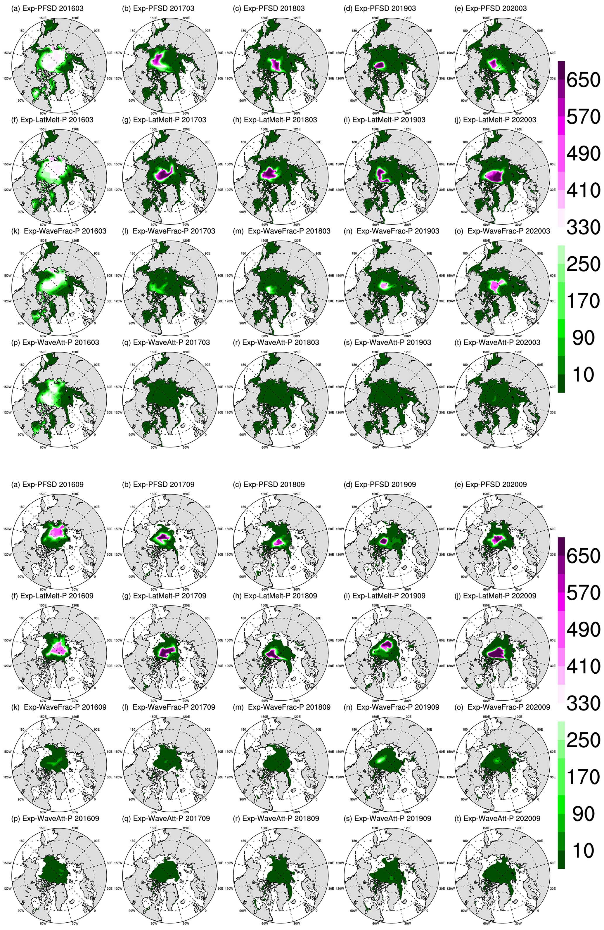
Figure 10The spatial distribution of the representative floe radius in March (upper panels) and September (bottom panels) of (a–e) Exp-PFSD, (f–j) Exp-LatMelt-P, (k–o) Exp-WaveFrac-P, and (p–t) Exp-WaveAtt-P for 2016–2020. Note that cells with less than 15 % ice concentration are treated as missing values. The date format is yyyymm (year followed by month).
4.4 Sensitivity to wave-attenuation parameterization
We have shown that ocean waves can alter the upper ocean through wave-enhanced mixing, which may affect sea ice locally (Fig. 8; see Sect. 4.1). The results from PF1 and PF2 experiments imply that the simulated wave parameters can determine how ice floes are fractured. As described in Sect. 2.1, we can choose different coefficients in Eq. (2) to control the wave attenuation rate of each frequency. In this section, we conduct experiments using R18 coefficients (see Sect. 3 and Table 2) to study the impacts of wave attenuation rate on Arctic sea ice simulation. The simulated sea ice area in Exp-WaveAtt-C (Fig. 2d, light-blue line) resembles that in Exp-CFSD (Fig. 2d, blue line) before 2019. After 2019, Exp-WaveAtt-C simulates smaller SIA compared to Exp-CFSD. Since both Exp-CFSD and Exp-WaveAtt-C use constant floe size, which allows us to neglect the effect of the spatial distribution of floe size and the MP87 scheme, which, in turn, makes lateral melt have a negligible contribution (Fig. S10d), basal melt is the primary factor for the ocean-induced ice melt during the entire period (Figs. 3a, f and S10e). The strength of basal melt in Exp-WaveAtt-C is weaker than that in Exp-CFSD from April 2018 to January 2020 (Fig. S10c). Basal growth of Exp-WaveAtt-C is also smaller than that of Exp-CFSD in the winters of 2017/18 and 2018/19 (Fig. S10f). Compared to Exp-CFSD, Exp-WaveAtt-C shows stronger top melt in the summer of 2018 (Fig. S10b). The combined effects of the above processes lead to a thinner ice state in Exp-WaveAtt-C before and during the 2018/19 winter (Fig. S10a). The thinner state of Exp-WaveAtt-C in the winter of 2018/19 causes more open water to be created by basal melt (regardless of its smaller magnitude) and thus smaller SIA (Fig. 2d), which is also shown in the thermally induced ice area changes whereby Exp-WaveAtt-C has a smaller magnitude in the corresponding period (Fig. 6d). As discussed in Sect. 4.1, top melt and basal growth are in good agreement with the ice–atmosphere heat flux (Figs. S10, S11a). That is, the ice mass and area changes described above are mainly driven by the ice–atmosphere heat flux associated with the atmospheric responses to the changes in ocean wave conditions.
Differently from the M14 experiments, the simulated SIAs of Exp-WaveAtt-C (light-blue line) and Exp-WaveAtt-P (yellow line) show relatively similar evolution during 2016–2020 (Fig. 2d). The R18 coefficients represent weaker wave attenuation relative to the M14 coefficients. Thus, ocean waves in the R18 experiments are expected to transmit further into the ice pack while maintaining relatively high wave energy. To quantify to what extent the ice can be affected by ocean waves, we calculate the wave-affected extent (WAE), which is defined as the sum of the area of cells with ice concentration greater than 15 % and significant wave height greater than 30 cm (Cooper et al., 2022). Figure 11 shows the evolution of WAE for the M14 and R18 experiments with a 15 d running average to smooth the high-frequency changes in wave conditions. The weaker attenuation in Exp-WaveAtt-C and Exp-WaveAtt-P results in generally larger WAE compared to Exp-CFSD and Exp-PFSD (as well as all previous experiments with M14 coefficients, not shown). The direct impact of larger WAE in Exp-WaveAtt-P is that the representative floe radius is mostly smaller than 10 m (fully fractured by ocean waves) (Fig. 10p–t). The decreasing tendency of the floe radius due to wave fracturing is the dominant factor contributing to the fully fractured condition (Fig. S7). Similarly to Exp-WaveFrac-P, the fully fractured condition does not lead to stronger ocean-induced melt due to limited oceanic energy (Figs. 3b, e, g and S10e).
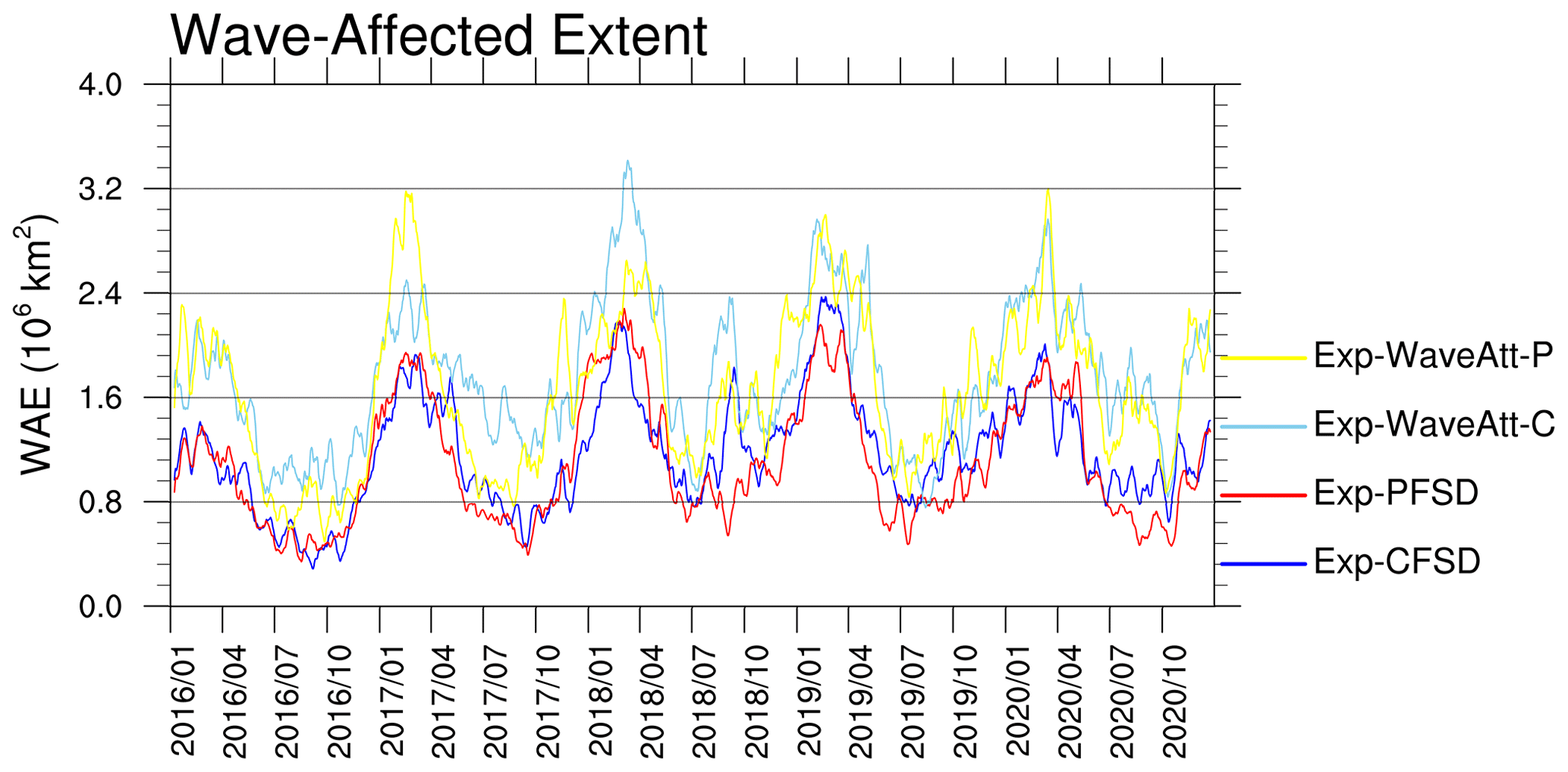
Figure 11Time series (15 d running average) of the Arctic wave-affected extent for Exp-CFSD (blue line), Exp-PFSD (red line), Exp-WaveAtt-C (light-blue line), and Exp-WaveAtt-P (yellow line). The date format is year/month.
This study investigates the impacts of ocean waves on Arctic sea ice simulation based on a newly developed atmosphere–ocean–wave–sea ice coupled model, which is built on the Coupled Arctic Prediction System (CAPS) by coupling Simulating WAves Nearshore (SWAN) and the implementation of the modified joint floe size and thickness distribution (FSTD). A set of pan-Arctic experiments with different configurations of FSD-related processes are performed for the period 2016–2020. Specifically, we examine the contrasting behaviors of sea ice between constant and prognostic floe size, the responses of sea ice to different lateral melting rate formulations, and the sensitivity of sea ice to the simulated wave parameters under the atmosphere–ocean–wave–sea ice coupled framework.
The results of FSD-fixed and FSD-varied experiments show that the simulated sea ice area is generally lower with smaller floe size associated with physical processes that change FSD. According to sea ice mass budget analysis, smaller floe size contributes to increased lateral melt, but its effect is reduced by decreased basal melt. The combined effects of lateral and basal melt associated with smaller floe size result in more ice melt by the ocean energy, which is a result similar to those of previous studies (e.g., Bateson et al., 2022; Roach et al., 2019; Smith et al., 2022). The simulations in Smith et al. (2022) with varying lateral melting strength based on the Community Earth System Model Version 2 (CESM2) with a slab-ocean model showed minimal change in frazil ice formation. In our simulation with a full ocean model, the ocean enhanced ice melt, though it is partially balanced by increased frazil ice formation due to the depletion of melting potential in the surface layer. This suggests negative feedback from the full ocean physics. Our simulations also show that the prevalence of small floes does not necessarily lead to stronger ice melting due to limited oceanic energy. To further illustrate the constraining role of limited oceanic energy, the mixed layer depths (MLDs) based on a 0.1 °C difference relative to the surface temperature (e.g., Courtois et al., 2017, their Table 2) for Exp-CFSD and Exp-PFSD are shown in Fig. 12. In general, Exp-CFSD and Exp-PFSD (as well as other experiments, not shown) exhibit similar evolution of MLD; that is, MLD is deeper (up to 150 m) in March and shallower (up to 80 m) in September. MLD in the open waters is broadly similar across all experiments, and MLD near the ice edge (15 % ice concentration, black contour in Fig. 12) is shallower (10–30 m) relative to other areas. In March, MLDs under ice-covered areas become deeper as lead time increases. To calculate the heat content within MLD, the same approach for calculating melting potential in the ROMS model is used, which is defined as the vertical integral from the surface to MLD of the difference between the ocean temperature and freezing point. The calculated values of heat content and melting potential have the same unit (W m−2) and directionality (positive downwards) as ice–ocean heat flux, and they represent the “maximum” heat flux that the ice can extract. Figures 13 and 14 show the heat content of MLD and melting potential for Exp-CFSD and Exp-PFSD in March and September. As shown in Figs. 13–14, Exp-PFSD shows less melting potential (0–5 m) and heat content within MLD under ice-covered areas compared to Exp-CFSD. These features are more pronounced in September than in March. Also, heat content in MLD near the ice edge of Exp-PFSD reduces more than other ice-covered areas compared to that of Exp-CFSD, suggesting the role of ice–ocean heat flux. Figures 13 and 14 further support the constraining role of limited oceanic energy in ice melting with respect to varied floe size not only in the surface layer (i.e., melting potential) but also in the mixed layer.
Figure 12Monthly mean of MLD in March (top panel) and September (bottom panel) of Exp-CFSD and Exp-PFSD for 2016–2020. Note that the black contour represents the average location of 15 % ice concentration. The date format is yyyymm (year followed by month).
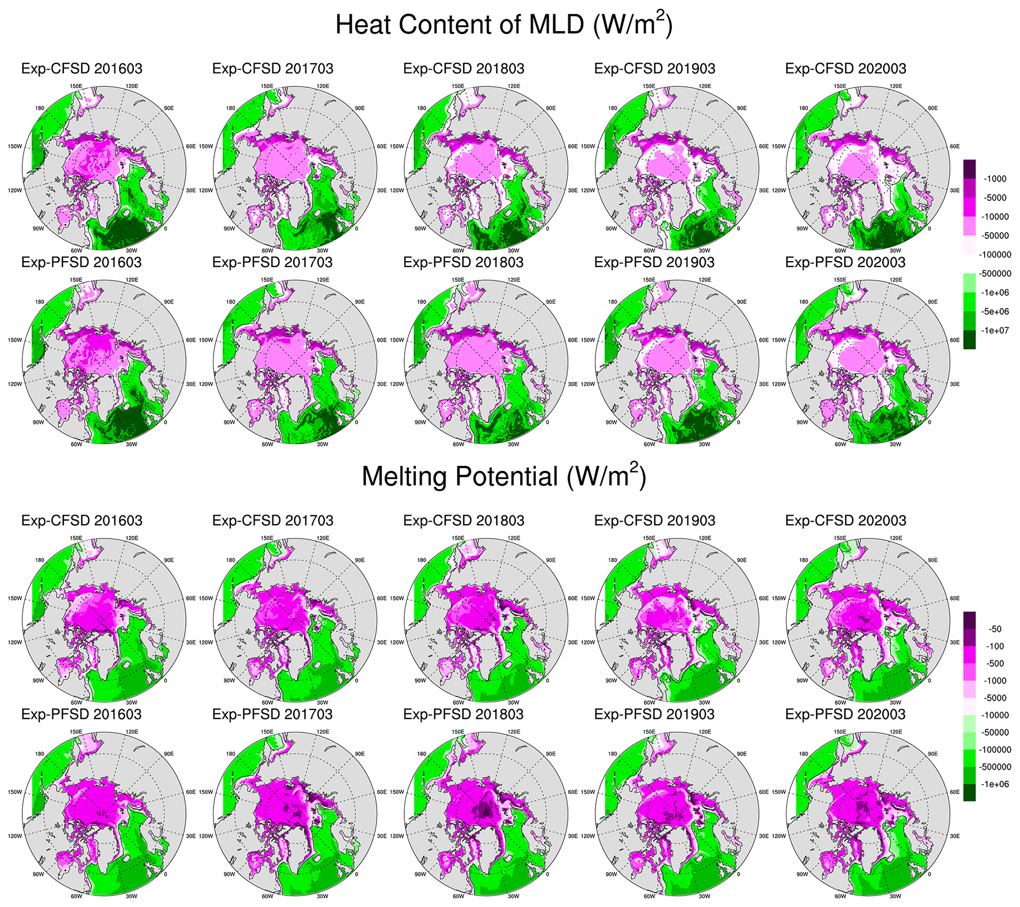
Figure 13March-averaged heat content of MLD (top panel) and melting potential (bottom panel) of Exp-CFSD and Exp-PFSD for 2016–2020. Note that the black contour represents the average location of 15 % ice concentration. The date format is yyyymm (year followed by month).
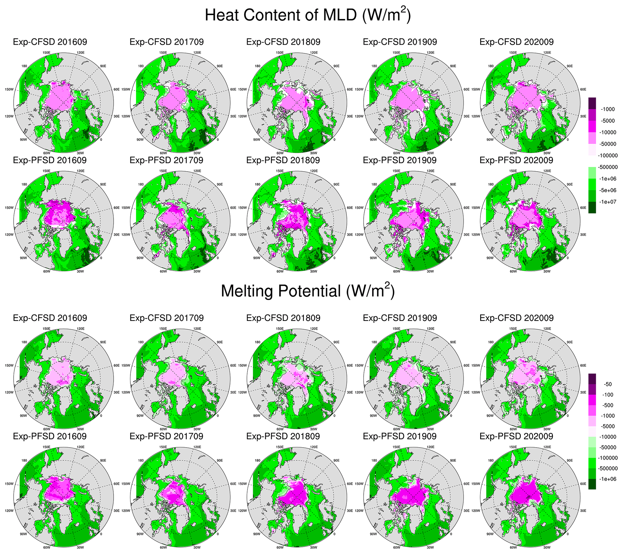
Figure 14The same as Fig. 13 but for September-averaged values. The date format is yyyymm (year followed by month).
Our fully coupled simulations also show that atmospheric states respond to changing ice distributions and then modify the energy budget at the ice surface that determines top melt in summer and basal growth in winter. The FSD-varied experiments, in general, show more energy loss from ice to the atmosphere in winter, and all experiments show year-to-year variations in energy gain for sea ice in summer.
The depletion of ocean energy in the surface layer and enhanced frazil ice formation are the direct responses to the changes in ice–ocean coupling with the prognostic FSD. The fractured sea ice enlarges the ice–ocean heat flux while the freezing temperature is still determined by the sea surface salinity in the ocean model. However, the local salinity at the ice–ocean interface can be significantly lower than sea surface salinity, and thus there is a higher freezing temperature locally due to the meltwater from sea ice (e.g., the false bottom; Notz et al., 2003). Schmidt et al. (2004) proposed the ice–ocean heat flux formulation that considers the local salinity equilibrium, but its formulation is only for the ice-bottom interface. The generalization of ice–ocean heat flux with the consideration of the local salinity equilibrium for both the bottom and lateral interface might yield a more realistic ice–ocean coupled simulation. Although the lateral melting rate formulation does not have a major effect on the simulated floe size distribution, the simulated sea ice area and ice mass budget are sensitive to the choice of the formulation. The lateral melting rate formulations applied in this study as well as previous laboratory results are not related to the ice properties (i.e., ice thickness and floe size; Josberger and Martin, 1981; Maykut and Perovich, 1987; Perovich, 1983). A recent laboratory study suggested that the lateral melting rate is a function of temperature difference and the ratio of floe size to ice thickness (Li et al., 2022). Smith et al. (2022) also suggested that Arctic sea ice simulation can be sensitive to the lateral melting rate of Perovich (1983) with different weights on each ice thickness category. Further studies are required to investigate improved lateral melting rate parameterization with observational constraints (e.g., data from the MOSAiC campaign in 2020; Nicolaus et al., 2021) within the prognostic FSD framework.
As discussed in Horvat and Tziperman (2015), FSTD is sensitive to the wave-attenuation coefficients. Our simulations also show substantially contrasting behaviors in the simulated floe size distribution associated with simulated wave parameters, suggesting that several aspects need further investigation. First, the empirical wave attenuation (i.e., IC4M2) may have reasonable performance in simulating the changes in the wave energy spectrum locally with specific ice conditions (e.g., Liu et al., 2020). However, the dissipation of wave energy varies spatially for the pan-Arctic-scale (as well as pan-Antarctic-scale) simulation with the different sea ice properties (i.e., ice concentration, ice thickness, floe size). Thus, a viscous boundary layer model (Liu et al., 1991) or a viscoelastic model (Wang and Shen, 2010) for wave attenuation, which provides spatially varied wave attenuation with respect to sea ice properties, might be able to give more realistic simulations in the wave-fracturing process and thus the floe size distribution. Also, the current implementation of sea ice effects in the SWAN model does not include the reflection and scattering due to sea ice, which redistribute the wave energy spatially and potentially change the wave-fracturing behavior. Second, the probability of floe fracturing Q(r) in both formulations applied in this study is uncertain. Both formulations result in floe fracturing into smaller floe size categories within a short time interval as long as the simulated wave parameters satisfy the yielding strain. This strong contribution in the wave-fracturing term is not easily balanced by the floe-welding term. The floe-welding term (Roach et al., 2018a, b) acts to reduce the floe number density so that it is less effective in increasing the representative floe radius if the floe is mostly fractured with the smallest floe size. Third, the attenuated wave energy by sea ice does not influence sea ice conditions in this study. As suggested by Longuet-Higgins and Steward (1962), the attenuated wave energy is transferred into the ocean (as we described in Sect. 3 for wave-enhanced mixing) or sea ice. For sea ice, the transferred energy acts as a stress, called wave radiation stress (WRS), pushing sea ice into the direction of wave propagation. By including the WRS in the momentum equation of ice, the WRS can then affect sea ice drift (e.g., Boutin et al., 2020).
For quantitative applications (e.g., forecasting sea ice), more observations (especially ocean waves under sea ice and FSD) are needed to reduce uncertainties in the atmosphere–ocean–wave–sea ice coupled model, particularly wave-related processes in ice-covered regions. Horvat et al. (2019) developed a new technique to retrieve pan-Arctic-scale FSD climatology and seasonal cycle from the CryoSat-2 radar altimeter, and this method can resolve floe size from 300 m to 100 km and potentially up to a 20 m scale if applied to ICESat-2 data. ICESat-2 altimetry also provides a new opportunity to observe ocean waves in sea ice with hemispheric-scale coverage by directly observing the vertical displacements of the ice surface (e.g., Horvat et al., 2020). In situ observations, despite their limited spatial coverage, are valuable wave spectrum measurements for wave-physics validation and improvement (e.g., Cooper et al., 2022; Liu et al., 2020).
The outputs of pan-Arctic simulations analyzed in this study are archived at https://doi.org/10.5281/zenodo.7922725 (Yang et al., 2023).
The supplement related to this article is available online at: https://doi.org/10.5194/tc-18-1215-2024-supplement.
CYY and JL designed the model experiments, developed the updated CAPS model, and wrote the manuscript. CYY conducted the experiments and analyzed the results. DC provided constructive feedback on the manuscript.
The contact author has declared that none of the authors has any competing interests.
Publisher's note: Copernicus Publications remains neutral with regard to jurisdictional claims made in the text, published maps, institutional affiliations, or any other geographical representation in this paper. While Copernicus Publications makes every effort to include appropriate place names, the final responsibility lies with the authors.
The authors acknowledge the National Centers for Environmental Information, the National Oceanic and Atmospheric Administration, for archiving and distributing the Climate Forecast System Version 2 operational analysis. The authors thank the editor, Xichen Li, and two anonymous reviewers for their helpful and constructive comments on the manuscript.
This research has been supported by the National Natural Science Foundation of China (grant nos. 42376237, 42006188), the National Key R&D Program of China (grant no. 2018YFA0605901), and the Innovation Group Project of Southern Marine Science and Engineering Guangdong Laboratory (Zhuhai) (grant no. 311021008).
This paper was edited by Xichen Li and reviewed by two anonymous referees.
Asplin, M. G., Scharien, R., Else, B., Howell, S., Barber, D. G., Papakyriakou, T., and Prinsenberg, S.: Implications of fractured Arctic perennial ice cover on thermodynamic and dynamic sea ice processes, J. Geophys. Res.-Oceans, 119, 2327–2343, https://doi.org/10.1002/2013JC009557, 2014.
Bai, Q. and Bai, Y.: 7 – Hydrodynamics around Pipes, Subsea Pipeline Design, Analysis, and Installation, Gulf Professional Publishing, 153–170, https://doi.org/10.1016/B978-0-12-386888-6.00007-9, 2014.
Bateson, A. W., Feltham, D. L., Schröder, D., Hosekova, L., Ridley, J. K., and Aksenov, Y.: Impact of sea ice floe size distribution on seasonal fragmentation and melt of Arctic sea ice, The Cryosphere, 14, 403–428, https://doi.org/10.5194/tc-14-403-2020, 2020.
Bateson, A. W., Feltham, D. L., Schröder, D., Wang, Y., Hwang, B., Ridley, J. K., and Aksenov, Y.: Sea ice floe size: its impact on pan-Arctic and local ice mass and required model complexity, The Cryosphere, 16, 2565–2593, https://doi.org/10.5194/tc-16-2565-2022, 2022.
Battjes, J. A. and Janssen, J. P. F. M.: Energy loss and set-up due to breaking of random waves, Coastal Engineering Proceedings, 1, 32, https://doi.org/10.9753/icce.v16.32, 1978.
Bennetts, L. G., O'Farrell, S., and Uotila, P.: Brief communication: Impacts of ocean-wave-induced breakup of Antarctic sea ice via thermodynamics in a stand-alone version of the CICE sea-ice model, The Cryosphere, 11, 1035–1040, https://doi.org/10.5194/tc-11-1035-2017, 2017.
Bitz, C. M. and Lipscomb, W. H.: An energy-conserving thermodynamic sea ice model for climate study. J. Geophys. Res.-Oceans, 104, 15669–15677, https://doi.org/10.1029/1999JC900100, 1999.
Blanchard-Wrigglesworth, E., Donohoe, A., Roach, L. A., DuVivier, A., and Bitz, C. M.:. High-frequency sea ice variability in observations and models, Geophys. Res. Lett., 48, e2020GL092356, https://doi.org/10.1029/2020GL092356, 2021.
Booij, N., Ris, R. C., and Holthuijsen, L. H.: A third-generation wave model for coastal regions. Part I: Model description and validation, J. Geophys. Res., 104, 7649–7666, https://doi.org/10.1029/98JC02622, 1999.
Boutin, G., Lique, C., Ardhuin, F., Rousset, C., Talandier, C., Accensi, M., and Girard-Ardhuin, F.: Towards a coupled model to investigate wave–sea ice interactions in the Arctic marginal ice zone, The Cryosphere, 14, 709–735, https://doi.org/10.5194/tc-14-709-2020, 2020.
Bretschneider, C. L.: Wave variability and wave spectra for wind-generated gravity waves, Technical Memorandum No. 118, Beach Erosion Board, Corps of Engineers, 196 pp., https://apps.dtic.mil/sti/tr/pdf/AD0227467.pdf (last access: 20 May 2023) 1959.
Briegleb, B. P. and Light, B.: A Delta-Eddington multiple scattering parameterization for solar radiation in the sea ice component of the Community Climate System Model, No. NCAR/TN-472+STR, University Corporation for Atmospheric Research, https://doi.org/10.5065/D6B27S71, 2007.
Casas-Prat, M. and Wang, X.: Sea ice retreat contributes to projected increases in extreme Arctic ocean surface waves, Geophys. Res. Lett., 47, e2020GL088100, https://doi.org/10.1029/2020GL088100, 2020.
Cassano, J. J., Higgins, M. E., and Seefeldt, M. W.: Performance of the Weather Research and Forecasting Model for Month-Long Pan-Arctic Simulations, Mon. Weather Rev., 139, 3469–3488, https://doi.org/10.1175/MWR-D-10-05065.1, 2011.
Chen, F. and Dudhia, J.: Coupling an advanced land surface–hydrology model with the Penn State–NCAR MM5 modeling system. Part I: Model implementation and sensitivity, Mon. Weather Rev., 129, 569–585, https://doi.org/10.1175/1520-0493(2001)129<0569:CAALSH>2.0.CO;2, 2001.
Cole, S. T., Toole, J. M., Lele, R., Timmermans, M.-L., Gallagher, S. G., Stanton, T. P., Shaw, W. J., Hwang, B., Maksym, T., Wilkinson, J. P., Ortiz, M., Graber, H., Rainville, L., Petty, A. A., Farrell, S. L., Richter-Menge, J. A., and Haas, C.: Ice and ocean velocity in the Arctic marginal ice zone: Ice roughness and momentum transfer, Elementa: Science of the Anthropocene, 5, 55, https://doi.org/10.1525/elementa.241, 2017.
Collins III, C. O., Rogers, W. E., Marchenko, A., and Babanin, A. V.: In situ measurements of an energetic wave event in the Arctic marginal ice zone, Geophys. Res. Lett., 42, 1863–1870, https://doi.org/10.1002/2015GL063063, 2015.
Collins III, C. O. and Rogers, W. E.: A Source Term for Wave Attenuation by Sea ice in WAVEWATCH III: IC4, NRL Report NRL/MR/7320–17-9726, 25 pp., https://www7320.nrlssc.navy.mil/pubs/2017/rogers-2017.pdf (last access: 20 May 2023), 2017.
Collins, W. D., Rasch, P. J., Boville, B. A., McCaa, J., Williamson, D. L., Kiehl, J. T., Briegleb, B. P., Bitz, C., Lin, S.-J., Zhang, M., and Dai, Y.: Description of the NCAR Community Atmosphere Model (CAM 3.0), No. NCAR/TN-464+STR, University Corporation for Atmospheric Research. https://doi.org/10.5065/D63N21CH, 2004.
Cooper, V. T., Roach, L. A., Thomson, J., Brenner, S. D., Smith, M. M., Meylan, M. H., and Bitz, C.M.: Wind waves in sea ice of the western Arctic and a global coupled wave-ice model, Philos. T. R. Soc. A, 380, 20210258, https://doi.org/10.1098/rsta.2021.0258, 2022.
Courtois, P., Hu, X., Pennelly, C., Spence, P., and Myers, P. G.: Mixed layer depth calculation in deep convection regions in ocean numerical models, Ocean Model., 120, 67–78, https://doi.org/10.1016/j.ocemod.2017.10.007, 2017.
Curry, J. A., Schramm, J. L., and Ebert, E. E.: Sea ice-albedo climate feedback mechanism, J. Climate, 8, 240–247, https://doi.org/10.1175/1520-0442(1995)008<0240:SIACFM>2.0.CO;2, 1995.
Dobrynin, M., Murawsky, J., and Yang, S.: Evolution of the global wind wave climate in CMIP5 experiments, Geophys. Res. Lett., 39, L18606, https://doi.org/10.1029/2012GL052843, 2012.
Dumont, D., Kohout, A., and Bertino, L.: A wave-based model for the marginal ice zone including a floe breaking parameterization, J. Geophys. Res., 116, C04001, https://doi.org/10.1029/2010JC006682, 2011.
Freitas, S. R., Grell, G. A., Molod, A., Thompson, M. A., Putman, W. M., Santos e Silva, C. M., and Souza, E. P.: Assessing the Grell–Freitas convection parameterization in the NASA GEOS modeling system, J. Adv. Model. Earth Sy., 10, 1266–1289, https://doi.org/10.1029/2017MS001251, 2018.
Gupta, M. and Thompson, A. F.: Regimes of sea-ice floe melt: Ice-ocean coupling at the submesoscales, J. Geophys. Res.-Oceans, 127, e2022JC018894, https://doi.org/10.1029/2022JC018894, 2022.
Hasselmann, S., Hasselmann, K., Allender, J. H., and Barnett, T. P.: Computations and parameterizations of the nonlinear energy transfer in a gravity wave spectrum. Part II: Parameterizations of the nonlinear transfer for application in wave models, J. Phys. Oceanogr., 15, 1378–1391, https://doi.org/10.1175/1520-0485(1985)015<1378:CAPOTN>2.0.CO;2, 1985.
Horvat, C.: Marginal ice zone fraction benchmarks sea ice climate model skill, Nat. Commun., 12, 2221, https://doi.org/10.1038/s41467-021-22004-7, 2021.
Horvat, C. and Tziperman, E.: A prognostic model of the sea-ice floe size and thickness distribution, The Cryosphere, 9, 2119–2134, https://doi.org/10.5194/tc-9-2119-2015, 2015.
Horvat, C., Tziperman, E., and Campin, J.-M.: Interaction of sea ice floe size, ocean eddies, and sea ice melting, Geophys. Res. Lett., 43, 8083–8090, https://doi.org/10.1002/2016GL069742, 2016.
Horvat, C., Roach, L. A., Tilling, R., Bitz, C. M., Fox-Kemper, B., Guider, C., Hill, K., Ridout, A., and Shepherd, A.: Estimating the sea ice floe size distribution using satellite altimetry: theory, climatology, and model comparison, The Cryosphere, 13, 2869–2885, https://doi.org/10.5194/tc-13-2869-2019, 2019.
Horvat, C., Blanchard-Wrigglesworth, E., and Petty, A. A.: Observing waves in sea ice with ICESat-2, Geophys. Res. Lett., 47, e2020GL087629, https://doi.org/10.1029/2020GL087629, 2020.
Hunke, E. C. and Dukowicz, J. K.: An elastic-viscous-plastic model for sea ice dynamics, J. Phys. Oceanogr., 27, 1849–67, https://doi.org/10.1175/1520-0485(1997)027<1849:AEVPMF>2.0.CO;2, 1997.
Josberger, E. G. and Martin, S.: A laboratory and theoretical study of the boundary layer adjacent to a vertical melting ice wall in salt water, J. Fluid Mech., 111, 439–473, https://doi.org/10.1017/S0022112081002450, 1981.
Kirby, J. T. and Chen, T. M.: Surface waves on vertically sheared flows: approximate dispersion relations, J. Geophys. Res., 94, 1013–1027, https://doi.org/10.1029/JC094iC01p01013, 1989.
Kohout, A., Williams, M. J., Dean, S. M., and Meylan, M.: Storm-induced sea-ice breakup and the implications for ice extent, Nature, 509, 604–607, https://doi.org/10.1038/nature13262, 2014.
Komen, G. J., Hasselmann, S., and Hasselmann, K.: On the existence of a fully developed wind-sea spectrum, J. Phys. Oceanogr., 14, 1271–1285, https://doi.org/10.1175/1520-0485(1984)014<1271:OTEOAF>2.0.CO;2, 1984.
Kumar, N., Voulgaris, G., Warner, J. C., and Olabarrieta, M.: Implementation of the vortex force formalism in the coupled ocean-atmosphere-wave-sediment transport (COAWST) modeling system for inner shelf and surf zone applications, Ocean Model., 47, 65–95, https://doi.org/10.1016/j.ocemod.2012.01.003, 2012.
Kwok, R.: Arctic sea ice thickness, volume, and multiyear ice coverage: Losses and coupled variability (1958–2018), Environ. Res. Lett., 13, 105005, https://doi.org/10.1088/1748-9326/aae3ec, 2018.
Langhorne, P. J., Squire, V. A., Fox, C., and Haskell, T. G.: Break-up of sea ice by ocean waves, Ann. Glaciol., 27, 438–442. https://doi.org/10.3189/S0260305500017869, 1998.
Leonard, B. and Mokhtari, S.: ULTRA-SHARP nonoscillatory convection schemes for high-speed steady multidimensional flow, NASA Technical Memorandum 102568, ICOMP-90-12, 54 pp., https://ntrs.nasa.gov/citations/19900012254 (last access: 20 May 2023), 1990.
Li, Z., Wang, Q., Li, G., Lu. P., Wang, Z., and Xie, F.: Laboratory Studies on the Parametrization Scheme of the Melting Rate of Ice–Air and Ice–Water Interfaces, Water, 14, 1775, https://doi.org/10.3390/w14111775, 2022.
Liang, X., Losch, M., Nerger, L., Mu, L., Yang, Q., and Liu, C.: Using sea surface temperature observations to constrain upper ocean properties in an Arctic sea ice-ocean data assimilation system, J. Geophys. Res.-Oceans, 124, 4727–4743, https://doi.org/10.1029/2019JC015073, 2019.
Lipscomb, W. H., Hunke, E. C., Maslowski, W., and Jakacki. J.: Ridging, strength, and stability in high-resolution sea ice models, J. Geophys. Res., 112, C03S91, https://doi.org/10.1029/2005JC003355, 2007.
Liu, Q., Babanin, A. V., Zieger, S., Young, I. R., and Guan, C.: Wind and Wave Climate in the Arctic Ocean as Observed by Altimeters, J. Climate 29, 7957–7975, https://doi.org/10.1175/JCLI-D-16-0219.1, 2016.
Longuet-Higgins, M. S. and Stewart, R. W.: Radiation stresses and mass transport in surface gravity waves with application to “surf beats”, J. Fluid Mech., 13, 481–504, https://doi.org/10.1017/S0022112062000877, 1962.
Loose, B., McGillis, W. R., Perovich, D., Zappa, C. J., and Schlosser, P.: A parameter model of gas exchange for the seasonal sea ice zone, Ocean Sci., 10, 17–28, https://doi.org/10.5194/os-10-17-2014, 2014.
Liu, A. K., Holt, B., and Vachon, P. W.: Wave propagation in the marginal ice zone: Model predictions and comparisons with buoy and synthetic aperture radar data, J. Geophys. Res., 96, 4605-4621, https://doi.org/10.1029/90JC02267, 1991.
Liu, D., Tsarau, A., Guan, C., and Shen, H. H.: Comparison of ice and wind-wave modules in WAVEWATCH III® in the Barents Sea, Cold Reg. Sci. Tech., 172, 103008, https://doi.org/10.1016/j.coldregions.2020.103008, 2020.
Lu, P., Li, Z., Cheng, B., and Leppäranta, M.: A parameterization of the ice-ocean drag coefficient, J. Geophys. Res., 116, C07019, https://doi.org/10.1029/2010JC006878, 2011.
Lukovich, J. V., Stroeve, J. C., Crawford, A., Hamilton, L., Tsamados, M., Heorton, H., and Massonnet, F.: Summer Extreme Cyclone Impacts on Arctic Sea Ice, J. Climate, 34, 4817–4834, https://doi.org/10.1175/JCLI-D-19-0925.1, 2021.
Madsen, O. S., Poon, Y.-K., and Graber, H. C.: Spectral wave attenuation by bottom friction: Theory, Coastal Engineering 1988, 492–504, https://doi.org/10.1061/9780872626874.035, 1988.
Martin, T., Tsamados, M., Schroeder, D., and Feltham, D. L.: The impact of variable sea ice roughness on changes in Arctic Ocean surface stress: A model study, J. Geophys. Res.-Oceans, 121, 1931–1952, https://doi.org/10.1002/2015JC011186, 2016.
Maykut, G. A. and McPhee, M. G.: Solar heating of the Arctic mixed layer, J. Geophys. Res.-Oceans, 100, 24691–24703, https://doi.org/10.1029/95JC02554, 1995.
Maykut, G. A. and Perovich, D. K.: The role of shortwave radiation in the summer decay of a sea ice cover, J. Geophys. Res.-Ocean., 92, 7032–7044, https://doi.org/10.1029/JC092iC07p07032, 1987.
Meylan, M. and Squire, V. A.: The response of ice floes to ocean waves, J. Geophys. Res., 99, 891–900, https://doi.org/10.1029/93JC02695, 1994.
Meylan, M. H., Bennetts, L. G., and A. L. Kohout: In situ measurements and analysis of ocean waves in the Antarctic marginal ice zone, Geophys. Res. Lett., 41, 5046–5051, https://doi.org/10.1002/2014GL060809, 2014.
Montiel, F., Squire, V., and Bennetts, L.: Attenuation and directional spreading of ocean wave spectra in the marginal ice zone, J. Fluid Mech., 790, 492-522, https://doi.org/10.1017/jfm.2016.21, 2016.
Morrison, H., Thompson, G., and Tatarskii, V.: Impact of Cloud Microphysics on the Development of Trailing Stratiform Precipitation in a Simulated Squall Line: Comparison of One- and Two-Moment Schemes, Mon. Weather Rev., 137, 991–1007, https://doi.org/10.1175/2008MWR2556.1, 2009.
Nakanishi, M. and Niino, H.: Development of an improved turbulence closure model for the atmospheric boundary layer, J. Meteor. Soc. Japan, 87, 895–912, https://doi.org/10.2151/jmsj.87.895, 2009.
National Centers for Environmental Prediction, National Weather Service, NOAA, and U.S. Department of Commerce: Climate Forecast System Version 2 (CFSv2) Operational Analaysis, NOAA National Centers for Environmental Information [data set], https://www.ncei.noaa.gov/access/metadata/landing-page/bin/iso?id=gov.noaa.ncdc:C00878, last access: 20 May 2023.
Naughten, K. A., Galton-Fenzi, B. K., Meissner, K. J., England, M. H., Brassington, G. B., Colberg, F., Hattermann, T., and Debernard, J. B.: Spurious sea ice formation caused by oscillatory ocean tracer advection schemes, Ocean Model., 116, 108–117, https://doi.org/10.1016/j.ocemod.2017.06.010, 2017.
Nicolaus, M., Perovich, D., Spreen, G., Granskog, M., Albedyll, L., Angelopoulos, M., Anhaus, P., Arndt, S., Belter, H., Bessonov, V., Birnbaum, G., Brauchle, J., Calmer, R., Cardellach, E., Cheng, B., Clemens-Sewall, D., Dadic, R., Damm, E., Boer, G., Demir, O., Dethloff, K., Divine, D., Fong, A., Fons, S., Frey, M., Fuchs, N., Gabarró, C., Gerland, S., Goessling, H., Gradinger, R., Haapala, J., Haas, C., Hamilton, J., Hannula, H.-R., Hendricks, S., Herber, A., Heuzé, C., Hoppmann, M., Høyland, K., Huntemann, M., Hutchings, J., Hwang, B., Itkin, P., Jacobi, H.-W., Jaggi, M., Jutila, A., Kaleschke, L., Katlein, C., Kolabutin, N., Krampe, D., Kristensen, S., Krumpen, T., Kurtz, N., Lampert, A., Lange, B., Lei, R., Light, B., Linhardt, F., Liston, G., Loose, B., Macfarlane, A., Mahmud, M., Matero, I., Maus, S., Morgenstern, A., Naderpour, R., Nandan, V., Niubom, A., Oggier, M., Oppelt, N., Pätzold, F., Perron, C., Petrovsky, T., Pirazzini, R., Polashenski, C., Rabe, B., Raphael, I., Regnery, J., Rex, M., Ricker, R., Riemann-Campe, K., Rinke, A., Rohde, J., Salganik, E., Scharien, R., Schiller, M., Schneebeli, M., Semmling, M., Shimanchuk, E., Shupe, M., Smith, M., Smolyanitsky, V., Sokolov, V., Stanton, T., Stroeve, J., Thielke, L., Timofeeva, A., Tonboe, R., Tavri, A., Tsamados, M., Wagner, D., Watkins, D., Webster, M., and Wendisch, M.: Overview of the MOSAiC expedition – Snow and Sea Ice, Elementa: Science of the Anthropocene, 10, 000046, https://doi.org/10.1525/elementa.2021.000046, 2021.
Notz, D., McPhee, M. G., Worster, M. G., Maykut, G. A., Schlünzen, K. H., and Eicken, H.: Impact of underwater-ice evolution on Arctic summer sea ice, J. Geophys. Res.-Oceans, 108, 3223, https://doi.org/10.1029/2001JC001173, 2003.
Notz, D., Jahn, A., Holland, M., Hunke, E., Massonnet, F., Stroeve, J., Tremblay, B., and Vancoppenolle, M.: The CMIP6 Sea-Ice Model Intercomparison Project (SIMIP): understanding sea ice through climate-model simulations, Geosci. Model Dev., 9, 3427–3446, https://doi.org/10.5194/gmd-9-3427-2016, 2016.
Parkinson, C. L. and Comiso, J. C.: On the 2012 record low Arctic sea ice cover: Combined impact of preconditioning and an August storm, Geophys. Res. Lett., 40, 1356–1361, https://doi.org/10.1002/grl.50349, 2013.
Peng, L., Zhang, X., Kim, J.-H., Cho, K.-H., Kim, B.-M., Wang, Z., and Tang, H.: Role of intense Arctic storm in accelerating summer sea ice melt: An in situ observational study, Geophys. Res. Lett., 48, e2021GL092714, https://doi.org/10.1029/2021GL092714, 2021.
Perovich, D.: On the summer decay of a sea ice cover, PhD dissertation, University of Washington, Seattle, 176 pp., 1983.
Perovich, D., Meier, W., Tshudi, M., Hendricks, S., Petty, A. A., Divine, D., Farrell, S., Gerland, S., Haas, C., Kaleschke, L., Pavlova, O., Ricker, R., Tian-Kunze, X., Webster, M., and Wood, K.: Sea Ice, Arctic Report Card 2020, edited by: Thoman, R. L., Richter-Menge, J., and Druckenmiller, M. L., https://doi.org/10.25923/n170-9h57, 2020.
Rampal, P., Weiss, J., and Marsan, D.: Positive trend in the mean speed and deformation rate of Arctic sea ice, 1979–2007, J. Geophys. Res., 114, C05013, https://doi.org/10.1029/2008JC005066, 2009.
Roach, L. A., Horvat, C., Dean, S. M., and Bitz, C. M.: An emergent sea ice floe size distribution in a global coupled ocean-sea ice model, J. Geophys. Res.-Oceans, 123, 4322–4337, https://doi.org/10.1029/2017JC013692, 2018a.
Roach, L. A., Smith, M. M., and Dean, S. M.: Quantifying growth of pancake sea ice floes using images from drifting buoys, J. Geophys. Res.-Oceans, 123, 2851–2866, https://doi.org/10.1002/2017JC013693, 2018b.
Roach, L. A., Bitz, C. M., Horvat, C., and Dean, S. M.: Advances in Modeling Interactions Between Sea Ice and Ocean Surface Waves, J. Adv. Model. Earth Sy., 11, 4167–4181, https://doi.org/10.1029/2019MS001836, 2019.
Rogers, W. E., Meylan, M. H., and Kohout, A. L.: Frequency Distribution of Dissipation of Energy of Ocean Waves by Sea Ice Using Data from Wave Array 3 of the ONR ”Sea State” Field Experiment, NRL Report NRL/MR/7322–18-9801, 25 pp., https://www7320.nrlssc.navy.mil/pubs/2018/rogers2-2018.pdf (last access: 20 May 2023), 2018.
Rogers, W. E.: Implementation of sea ice in the wave model SWAN, NRL Memorandum Report NRL/MR/7322–19-9874, 25 pp., https://www7320.nrlssc.navy.mil/pubs/2019/rogers2-2019.pdf (last access: 20 May 2023), 2019.
Rothrock, D. A. and Thorndike, A. S.: Measuring the sea ice floe size distribution, J. Geophys. Res., 89, 6477–6486, https://doi.org/10.1029/JC089iC04p06477, 1984.
Saha, S., Moorthi, S., Wu, X., Wang, J., Nadiga, S., Tripp, P., Behringer, D., Hou, Y., Chuang, H., Iredell, M., Ek, M., Meng, J., Yang, R., Mendez, M. P., van den Dool, H., Zhang, Q., Wang, W., Chen, M., and Becker, E.: The NCEP climate forecast system version 2, J. Climate, 27, 2185–2208, https://doi.org/10.1175/JCLI-D-12-00823.1, 2014.
Schäfer, M., Bierwirth, E., Ehrlich, A., Jäkel, E., and Wendisch, M.: Airborne observations and simulations of three-dimensional radiative interactions between Arctic boundary layer clouds and ice floes, Atmos. Chem. Phys., 15, 8147–8163, https://doi.org/10.5194/acp-15-8147-2015, 2015.
Schmidt, G. A., Bitz, C. M., Mikolajewicz, U., and Tremblay, L.-B.: Ice-ocean boundary conditions for coupled models, Ocean Model., 7, 59–74, https://doi.org/10.1016/S1463-5003(03)00030-1, 2004.
Sepp, M. and Jaagus, J.: Changes in the activity and tracks of Arctic cyclones, Climatic Change, 105, 577–595, https://doi.org/10.1007/s10584-010-9893-7, 2011.
Shchepetkin, A. F. and McWilliams, J. C.: The Regional Ocean Modeling System: A split-explicit, free-surface, topography following coordinates ocean model, Ocean Model., 9, 347–404, https://doi.org/10.1016/j.ocemod.2004.08.002, 2005.
Simmonds, I. and Rudeva, I.: The great Arctic cyclone of August 2012, Geophys. Res. Lett., 39, L23709, https://doi.org/10.1029/2012GL054259, 2012.
Smith, M. M., Holland, M., and Light, B.: Arctic sea ice sensitivity to lateral melting representation in a coupled climate model, The Cryosphere, 16, 419–434, https://doi.org/10.5194/tc-16-419-2022, 2022.
Spreen, G., Kwok, R., and Menemenlis, D.: Trends in Arctic sea ice drift and role of wind forcing: 1992–2009, Geophys. Res. Lett., 38, L19501, https://doi.org/10.1029/2011GL048970, 2011.
Squire, V. A.: Ocean Wave Interactions with Sea Ice: A Reappraisal, Annu. Rev. Fluid Mech., 52, 37–60, https://doi.org/10.1146/annurev-fluid-010719-060301, 2020.
Squire, V. A. and Montiel, F.: Evolution of Directional Wave Spectra in the Marginal Ice Zone: A New Model Tested with Legacy Data, J. Phys. Oceanogr., 46, 3121–3137, https://doi.org/10.1175/JPO-D-16-0118.1, 2016.
Steele, M.: Sea ice melting and floe geometry in a simple ice-ocean model, J. Geophys. Res., 97, 17729–17738, https://doi.org/10.1029/92JC01755, 1992.
Steele, M., Morison, J. H., and Untersteiner, N.: The partition of air-ice-ocean momentum exchange as a function of ice concentration, floe size, and draft, J. Geophys. Res., 94, 12739–12750, https://doi.org/10.1029/JC094iC09p12739, 1989.
Steer, A., Worby, A., and Heil, P.: Observed changes in sea-ice floe size distribution during early summer in the western Weddell Sea, Deep Sea Res. Pt. II, 55, 933–942, https://doi.org/10.1016/j.dsr2.2007.12.016, 2008.
Stern, D., P, Doyle, J. D., Barton, N. P., Finocchio, P. M., Komaromi, W. A., and Metzger, E. J.: The impact of an intense cyclone on short-term sea ice loss in a fully coupled atmosphere-ocean-ice model, Geophys. Res. Lett., 47, e2019GL085580, https://doi.org/10.1029/2019GL085580, 2020.
Stopa, J. E., Ardhuin, F., and Girard-Ardhuin, F.: Wave climate in the Arctic 1992–2014: seasonality and trends, The Cryosphere, 10, 1605–1629, https://doi.org/10.5194/tc-10-1605-2016, 2016.
Taylor, P. K. and Yelland, M. J.: The dependence of sea surface roughness on the height and steepness of the waves, J. Phys. Oceanogr., 31, 572–590, https://doi.org/10.1175/1520-0485(2001)031<0572:TDOSSR>2.0.CO;2, 2001.
Thomson, J. and Rogers, W. E.: Swell and sea in the emerging Arctic Ocean, Geophys. Res. Lett., 41, 3136–3140, https://doi.org/10.1002/2014GL059983, 2014.
Thorndike, A. S., Rothrock, D. A., Maykut, G. A., and Colony, R.: The thickness distribution of sea ice, J. Geophys. Res., 80, 4501–4513, https://doi.org/10.1029/JC080i033p04501, 1975.
Toyota, T., Takatsuji, S., and Nakayama, M.: Characteristics of sea ice floe size distribution in the seasonal ice zone, Geophys. Res. Lett., 33, L02616, https://doi.org/10.1029/2005GL024556, 2006.
Toyota, T., Haas, C., and Tamura, T.: Size distribution and shape properties of relatively small sea-ice floes in the Antarctic marginal ice zone in late winter, Deep Sea Res. Pt. II, 58, 1182–1193, https://doi.org/10.1016/j.dsr2.2010.10.034, 2011.
Tsamados, M., Feltham, D. L., Schroeder, D., Flocco, D., Farrell, S. L., Kurtz, N., Laxon, S. W., and Bacon, S.: Impact of Variable Atmospheric and Oceanic Form Drag on Simulations of Arctic Sea Ice, J. Phys. Oceanogr., 44, 5, 1329–1353, https://doi.org/10.1175/JPO-D-13-0215.1, 2014.
Tsamados, M., Feltham, D., Petty, A., Schroeder, D., and Flocco, D.: Processes controlling surface, bottom and lateral melt of Arctic sea ice in a state of the art sea ice model, Philos. T. R. Soc. A, 373, 20140167, https://doi.org/10.1098/rsta.2014.0167, 2015.
Tschudi, M. A., Stroeve, J. C., and Stewart, J. S.: Relating the age of Arctic sea ice to its thickness, as measured during NASA's ICESat and IceBridge campaigns, Remote Sensing, 8, 457, https://doi.org/10.3390/rs8060457, 2016.
Uchiyama, Y., McWilliams, J. C., and Shchepetkin, A. F.: Wave–current interaction in an oceanic circulation model with a vortex-force formalism: Application to the surf zone, Ocean Model., 34, 16–35, https://doi.org/10.1016/j.ocemod.2010.04.002, 2010.
Umlauf, L. and Burchard, H.: A generic length-scale equation for geophysical turbulence models, J. Marine Res., 61, 235–265, https://elischolar.library.yale.edu/journal_of_marine_research/9/ (last access: 20 May 2023), 2003.
Valkonen, E., Cassano, J., and Cassano, E.: Arctic cyclones and their interactions with the declining sea ice: A recent climatology, J. Geophys. Res.-Atmos., 126, e2020JD034366, https://doi.org/10.1029/2020JD034366, 2021.
Vella, D. and Wettlaufer, J. S.: Explaining the patterns formed by ice floe interactions, J. Geophys. Res., 113, C11011, https://doi.org/10.1029/2008JC004781, 2008.
Wang, R. and Shen, H. H.: Gravity waves propagating into an ice-covered ocean: A viscoelastic model, J. Geophys. Res., 115, C06024, https://doi.org/10.1029/2009JC005591, 2010.
Warner, J. C., Armstrong, B., He, R., and Zambon, J.: Development of a coupled ocean-atmosphere-wave-sediment transport (COAWST) modeling system, Ocean Modell., 35, 230–244, https://doi.org/10.1016/j.ocemod.2010.07.010, 2010.
Waseda, T., Webb, A., Sato, K., Inoue, J., Kohout, A., Penrose, B., and Penrose, S.: Correlated Increase of High Ocean Waves and Winds in the Ice-Free Waters of the Arctic Ocean, Sci. Rep., 8, 4489, https://doi.org/10.1038/s41598-018-22500-9, 2018.
Waseda, T., Nose, T., Kodaira, T., Sasmal, K., and Webb, A.: Climatic trends of extreme wave events caused by Arctic cyclones in the western Arctic Ocean, Polar Sci., 27, 100625, https://doi.org/10.1016/j.polar.2020.100625, 2021.
Weiss J. and Dansereau V.: Linking scales in sea ice mechanics. Philos. T. R. Soc. A, 375, 20150352, https://doi.org/10.1098/rsta.2015.0352, 2017.
Wenta, M. and Herman, A.: Area-Averaged Surface Moisture Flux over Fragmented Sea Ice: Floe Size Distribution Effects and the Associated Convection Structure within the Atmospheric Boundary Layer, Atmosphere, 10, 654, https://doi.org/10.3390/atmos10110654, 2019.
Wilchinsky, A. V., Feltham, D. L., and Hopkins, M. A.: Effect of shear rupture on aggregate scale formation in sea ice, J. Geophys. Res., 115, C10002, https://doi.org/10.1029/2009JC006043, 2010.
Yang, C.-Y., Liu, J., and Xu, S.: Seasonal Arctic sea ice prediction using a newly developed fully coupled regional model with the assimilation of satellite sea ice observations, J. Adv. Model. Earth Sy., 12, e2019MS001938, https://doi.org/10.1029/2019MS001938, 2020.
Yang, C.-Y., Liu, J., and Chen, D.: An improved regional coupled modeling system for Arctic sea ice simulation and prediction: a case study for 2018, Geosci. Model Dev., 15, 1155–1176, https://doi.org/10.5194/gmd-15-1155-2022, 2022.
Yang, C.-Y., Liu, J., and Chen, D.: The simulated outputs analyzed in the article: “Understanding the influences of ocean waves on Arctic sea ice simulation: a modeling study with an atmosphere-ocean-wave-sea ice coupled model”, Zenodo [data set], https://doi.org/10.5281/zenodo.7922725, 2023.
Zahn, M., Akperov, M., Rinke, A., Feser, F., and Mokhov, I. I.: Trends of cyclone characteristics in the Arctic and their patterns from different reanalysis data, J. Geophys. Res.-Atmos., 123, 2737–2751, https://doi.org/10.1002/2017JD027439, 2018.
Zhang, F., Pang, X., Lei, R., Zhai, M., Zhao, X., and Cai, Q.: Arctic sea ice motion change and response to atmospheric forcing between 1979 and 2019, Int. J. Climatol., 42, 1854–1876, https://doi.org/10.1002/joc.7340, 2022.
Zhang, J., Lindsay, R., Schweiger, A., and Steele, M.: The impact of an intense summer cyclone on 2012 Arctic sea ice retreat, Geophys. Res. Lett., 40, 720–726, https://doi.org/10.1002/grl.50190, 2013.
Zhang, J., Schweiger, A., Steele, M., and Stern, H.: Sea ice floe size distribution in the marginal ice zone: Theory and numerical experiments, J. Geophys. Res.-Oceans, 120, 3484–3498, https://doi.org/10.1002/2015JC010770, 2015.
Zhang, J., Stern, H., Hwang, B., Schweiger, A., Steele, M., Stark, M., and Graber, H. C.: Modeling the seasonal evolution of the Arctic sea ice floe size distribution, Elementa: Science of the Anthropocene, 4, 000126, https://doi.org/10.12952/journal.elementa.000126, 2016.