the Creative Commons Attribution 4.0 License.
the Creative Commons Attribution 4.0 License.
 | 01 Mar 2023
Spatio-temporal reconstruction of winter glacier mass balance in the Alps, Scandinavia, Central Asia and western Canada (1981–2019) using climate reanalyses and machine learning
Matteo Guidicelli
Matthias Huss
Marco Gabella
Nadine Salzmann
Spatio-temporal reconstruction of winter glacier mass balance is important for assessing long-term impacts of climate change. However, high-altitude regions significantly lack reliable observations, which is limiting the calibration of glaciological and hydrological models. Reanalysis products provide estimates of snow precipitation also for remote high-mountain regions, but this data come with inherent uncertainty, and assessing their biases is difficult given the low quantity and quality of available (long-term) in situ observations. In this study, we aim at improving knowledge on the spatio-temporal variations in winter glacier mass balance by exploring the combination of data from reanalyses and direct snow accumulation observations on glaciers using machine learning. We use the winter mass balance data of 95 glaciers distributed over the European Alps, western Canada, Central Asia and Scandinavia and compare them with the total precipitation from the ERA5 and the MERRA-2 reanalysis products during the snow accumulation seasons from 1981 until 2019. We develop and apply a machine learning model to adjust the precipitation from the reanalysis products along the elevation profile of the glaciers and consequently to reconstruct the winter mass balance in both space (for glaciers without observational data) and time (filling observational data gaps). The employed machine learning model is a gradient boosting regressor (GBR), which combines several meteorological variables from the reanalyses (e.g. air temperature, relative humidity) with topographical parameters. These GBR-derived estimates are evaluated against the winter mass balance data using (i) independent glaciers (site-independent GBR) and (ii) independent accumulation seasons (season-independent GBR). Both approaches resulted in reduced biases and increased correlation between the precipitation of the original reanalyses and the winter mass balance data of the glaciers. Generally, the GBR models have also shown a good representation of the spatial (vertical elevation intervals) and temporal (years) variability of the winter mass balance on individual glaciers.
- Article
(7621 KB) - Full-text XML
-
Supplement
(484 KB) - BibTeX
- EndNote


Climate change considerably alters the high-mountain cryosphere (e.g. Beniston, 2012; Vorkauf et al., 2021; Marty, 2008; Beniston et al., 2018; Bormann et al., 2018). Vanishing glaciers and changes in the seasonal snow regime significantly change water availability and storage capacities in worldwide high-mountain regions, impacting adjacent lowlands far away (e.g. Viviroli et al., 2007; Immerzeel et al., 2020). Cryospheric hazards such as slope failures and glacier lake outburst floods (e.g. Gobiet et al., 2014; Rasul and Molden, 2019) are other impacts of climate change in mountain regions, with direct adverse impacts on mountain societies (e.g. Adger et al., 2003; Hock et al., 2019). The rate and magnitude of cryospheric changes significantly depend on the evolution of the high-altitude precipitation regime. The elevation dependency of precipitation trends is however unclear; while precipitation trends from station observations often show an inconsistent picture with no systematic changes with elevation, gridded datasets show reduced precipitation increases at higher elevations (e.g. Pepin et al., 2022). It is thus crucial to improve our understanding of the local high-altitude climate–cryosphere interaction (e.g. Stone et al., 2013; Salzmann et al., 2014; Huss et al., 2017; Barandun et al., 2020). However, at the local scale and particularly at very high altitudes, snow and precipitation in situ observations are typically very scarce, spatially not optimally distributed, with low temporal resolution, too short in time, or with important gaps caused by technical challenges and difficult accessibility and thus complicated and lavish maintenance (e.g. Beniston et al., 2012; Tapiador et al., 2012). This is an important limitation for studies focusing on the long-term effects of climate change at the high-mountain cryosphere, which require snow accumulation data covering decadal periods (e.g. Seiz et al., 2010). At very high altitudes, mostly only measured snow water equivalent (SWE) as the cumulative snow accumulation on glaciers is available. Measurements of SWE on glaciers are typically used for the determination of winter mass balance (Cogley et al., 2011), an important variable in international glacier monitoring (e.g. Zemp et al., 2013). The main process of snow accumulation is the total precipitation received by the glacier during the accumulation season. Since melting is often negligible during this time period, SWE on glaciers represents a reliable measure of local winter precipitation and was thus used for a comparison with precipitation products in different studies (e.g. Gugerli et al., 2020; Guidicelli et al., 2021). However, other processes such as deposition of hoar, freezing rain or snow drift caused by winds and avalanching can also influence the accumulation (Dadic et al., 2010; Gascoin et al., 2013).
Worldwide spatio-temporally continuous information on precipitation, snow depth and SWE is also provided by climate reanalyses that merge physical laws with the assimilated satellite and ground observations (e.g. Hersbach et al., 2020; Gelaro et al., 2017). However, the performance of reanalysis results can vary greatly depending on the region and the elevation range of interest (Sun et al., 2018). Large biases in reanalysis precipitation are particularly found in high-mountain regions (e.g. Liu and Margulis, 2019; Zandler et al., 2019). The scarcity of observations available for assimilation and the coarse resolution of such models limit their accuracy in areas of complex topography and their suitability for studies at a local scale (e.g. Salzmann and Mearns, 2012, (for snow)).
Thus, the further development of techniques to spatially and/or temporally transfer the available observational series between sites and/or filling data gaps is critical and urgently needed (e.g. Salzmann et al., 2014). Downscaling of precipitation estimates of reanalyses is thereby a necessary step to represent the local conditions in high-mountain regions. Different statistical and dynamical downscaling methods exist (see Maraun et al., 2010), which have also been employed and evaluated over glacierized regions (e.g. Mölg and Kaser, 2011). For instance, Liston and Elder (2006) developed a quasi-physically based meteorological model to produce high-resolution (30 m to 1 km horizontal grid) atmospheric forcings for several variables, where the precipitation adjustment is a non-linear function of the elevation difference between the grid and the point of interest. The same equation was used by Gupta and Tarboton (2016), who proposed an approach to downscale the MERRA (Rienecker et al., 2011) variables. They obtained a Nash–Sutcliffe efficiency greater than 0.70 for downscaled monthly precipitation at 173 Snow Telemetry (SNOTEL) sites. Fiddes and Gruber (2014) adapted this method for the Swiss Alps by including a climatological parameter based on the Alpine precipitation dataset provided by the Climatic Research Unit (gridded monthly precipitation totals at 10 arcmin resolution over the Alps, for the period 1800–2003). Their product allowed for improving the purely lapse-rate-based approach of Liston and Elder (2006), obtaining a correlation coefficient of 0.6 (versus 0.5) against the annual precipitation observed at 40 MeteoSwiss automatic meteorological network (ANETZ) stations. Recently, machine learning methods have demonstrated their high performance to statistically downscale reanalyses (and global climate models) estimates of precipitation and other meteorological variables, from sub-daily and daily (e.g. Serifi et al., 2021; Wang et al., 2021) to monthly and seasonal (e.g. Sachindra et al., 2018; Najafi et al., 2011; Sun and Tang, 2020) resolution. However, downscaling methods for snow (and precipitation) are rarely assessed at very high elevations, mainly due to the scarcity of ground observations. Consequently, long-term effects of climate change on the snowpack at very high elevations are not well understood yet (e.g. Seiz et al., 2010).
In this study, we thus aim at analysing total precipitation biases of reanalysis datasets (ERA5 and MERRA-2) over the snow accumulation season on glaciers, i.e. at the highest elevations of different mountain ranges. The precipitation estimates are compared with the winter glacier mass balance data covering a period of up to 39 years from 95 glaciers in the European Alps, Scandinavia, Central Asia and western Canada. The selection of these regions and glaciers depends on the data consistency and availability (see Sect. 2.2). Ultimately, we aim at reconstructing the winter glacier mass balance from partial information. In order to achieve this goal, we develop and evaluate a machine learning approach based on gradient boosting regressor (GBR) models (see Friedman, 2001) to adjust the total precipitation of reanalysis (main driver of snow accumulation) along the elevation profiles of the glaciers. More specifically, the GBR models aim at allowing the spatio-temporal transferability of the learned information over the 95 glaciers to other glaciers with no ground observations and/or filling gaps of observational series. The new information provided by our exploratory study is expected to be helpful to improve the calibration of glaciological and hydrological models in observation-scarce regions.

The study was conducted on 95 glaciers located in the Alps, Scandinavia, Central Asia and western Canada (Fig. 1), where the longest time series and the highest density of winter glacier mass balance data are available. In the following, we describe the different data sources used in the study.
2.1 Reanalysis data
We used data from ERA5 and MERRA-2 reanalyses, since these are currently among the most widely used reanalysis products, providing the highest spatial resolution and covering the longest time period in all the regions of our study.
2.1.1 ERA5
ERA5 is the fifth generation of the European Centre for Medium-Range Weather Forecasts atmospheric reanalyses of the global climate (see Hersbach et al., 2020 for more information). In this study, we used several variables from the ERA5 hourly data on single levels from 1979 to present (Hersbach et al., 2018b) and the ERA5 hourly data on pressure levels from 1979 to present (Hersbach et al., 2018a), all with a spatial resolution of 0.25∘,× 0.25∘ (∼30 km). All variables were resampled on a daily timescale before usage. The list of variables selected for the analysis is reported in Table B1. The ERA5 precipitation variable used in the study is total precipitation (tp) from the ERA5 single levels.
2.1.2 MERRA-2
MERRA-2 is the second version of the Modern-Era Retrospective Analysis for Research and Applications (see Gelaro et al., 2017, for more information). In this study, we used several variables from the MERRA-2 Land Surface Diagnostics (Global Modeling and Assimilation Office (GMAO), 2015b), the MERRA-2 Single-Level Diagnostics (Global Modeling and Assimilation Office (GMAO), 2015c) and the MERRA-2 Analysed Meteorological Fields (Global Modeling and Assimilation Office (GMAO), 2015a). All variables have a spatial resolution of 0.5∘ × 0.625∘ (∼50 km), and we resampled them on a daily timescale before usage. The list of the selected variables is reported in Table B2. The MERRA-2 precipitation variable used in the study is total precipitation (PRECTOTLAND) from the MERRA-2 Land Surface Diagnostics.
2.2 Winter mass balance data
The World Glacier Monitoring Service (WGMS) compiles and publishes standardized observations on changes in mass, volume, length and area of glaciers collected by national monitoring programmes and local observers around the world (glacier fluctuations; see Zemp et al., 2021 for more details). The data compilation provided by the WGMS based on dozens of detailed national monitoring programmes is unique in terms of providing consistent in situ data in different regions of the world at the highest elevation of mountain ranges, i.e. on glaciers that can be used for comparison with precipitation datasets.
Thus, we used the winter mass balance data separated per elevation intervals (EE-MASS-BALANCE data sheet in WGMS, 2021), and we refer to them as Bw in this study. Point observations are also available (EEE-MASS-BALANCE POINT data sheet in WGMS, 2021) but are not used in this study because of the smaller number of glaciers with complete information reported (observation dates, elevation, coordinates). We only considered the Bw data where the elevation interval is indicated in the WGMS database. The glacier area related to each elevation interval was also used to weight the Bw data. In addition, we considered the average slope and aspect of the glaciers by using the information provided in the Randolph Glacier Inventory version 6 (RGI Consortium, 2017).
The winter mass balance is the result of the balance between the gain of snow which accumulates over the glacier, as well as refreezing of liquid water within the snowpack, and the loss caused by melting and sublimation over the accumulation season. Other processes such as snow drift caused by winds can also influence the accumulation. The amount of snow melt is typically minor compared to the snow accumulation and thus negligible in the comparison with the precipitation totals performed in this study. Snow accumulation is expressed in SWE (e.g. Østrem and Brugman, 1991), which is calculated by multiplying the measured snow depth with the respective bulk density of the snowpack. The snow depth is typically measured with a snow probe or ground-penetrating radar, while the snow density is usually measured in snow pits or by coring and is subsequently extrapolated to all observations on a glacier. The WGMS database only provides information on Bw but does not generally allow tracing whether density was directly measured or not.
The Bw data used in this study correspond to the mean winter balance for the glacier area within the respective elevation interval. Various spatial extrapolation techniques were applied by the national observers to infer elevation band average snow accumulation from the (sparse) point observations, which can be challenging due to important local-scale variability in snow depth (e.g. Dadic et al., 2010; Helfricht et al., 2014; Sold et al., 2016). Unfortunately, the WGMS database does not allow tracing the methods used, hence, resulting in an uncertainty that is difficult to be estimated. Often, no direct snow depth and density observations are available at the most extreme elevations of the glaciers because of high surface slopes and difficult accessibility. The employed techniques in the framework of the Swiss national programme Glacier Monitoring Switzerland (GLAMOS), which provides the data of the Swiss sites to WGMS) are described in Huss et al. (2021). The impact of the inter- and extrapolation of direct SWE measurements acquired on glaciers to obtain Bw data used in this study on our results is discussed in Sect. 5.2.5.
The starting date of the accumulation season is not precisely known but often determined with a stratigraphic system (i.e. since the date of the minimum surface in the previous summer) (e.g. Mayo et al., 1972; Cogley et al., 2011). The date of the minimum surface varies between the years and also across the glacier. In fact, snow accumulation starts typically later at lower elevations than at higher elevations (Huss et al., 2009). However, in this study we used a unique starting date for the entire glacier according to the information provided in the WGMS database. The end of the season is determined by the day of the snow survey that is indicated in the WGMS database. In this study, we cumulated precipitation amounts over the accumulation season. The impact of the date considered the beginning of the accumulation season on our results is discussed in Sect. 5.2.5.
First, we derived the total or average of all variables provided by the reanalyses for the entire accumulation season. Subsequently, a machine learning model to adjust the total precipitation (see Sect. 2.1.1 and 2.1.2) of the reanalyses over glaciers for the accumulation season was developed to reconstruct the Bw along the elevation profile of the glaciers. We use a gradient boosting regressor (GBR), which makes use of several meteorological variables (original and downscaled) and topographical parameters as input variables (predictors). The list of predictors required by the GBR is summarized in Table B3, while the variable names are described in Tables B1 (ERA5) and B2 (MERRA-2). In principle, a different adjustment factor of precipitation might be needed depending on the precipitation phase. However, as we only adjust the total precipitation occurring during the accumulation season, the adjustment factors used here represent the “average” adjustment factor of all precipitation events. Moreover, the snowfall variable was used as a predictor in order to enable the GBR model to learn that a different “average” adjustment factor must be applied depending on the fraction of snowfall and total precipitation (i.e. depending on the main precipitation phase during the accumulation season).
The applied methods to downscale the meteorological variables used by the GBR model as predictors are described below.
3.1 Downscaling temperature and relative humidity
In addition to the original variables (all “constants”, all “single level” and all “land surface” variables in Tables B1 and B2), the GBR requires some downscaled variables of the reanalyses as predictors at the glacier elevation intervals (see Table B3), including air temperature, dew point temperature and relative humidity (for MERRA-2 and ERA5), vertical velocity of air motion (for ERA5 only), and specific humidity (for MERRA-2 only). The downscaling procedure was applied at a daily resolution using a linear interpolation between the values of the two closest pressure levels to the centre of the elevation intervals of the Bw data of the glaciers. This downscaling approach is illustrated in the Supplement (Fig. S1).
If information regarding the relative humidity was not directly provided by the reanalyses, we applied approaches presented by Liston and Elder (2006) and Gupta and Tarboton (2016) to derive it. The applied equations are described in Appendix A.
3.2 Downscaling precipitation
The total precipitation over the accumulation season was considered the main driver of Bw. Thus, in order to derive Bw estimates over the glaciers, we built a machine learning model that adjusts the total precipitation of reanalysis along the elevation profile of the glaciers. In this study, we also applied a pre-existing lapse-rate-based approach (not data-informed) for precipitation downscaling that we considered a benchmark. The approaches are described below, and the results obtained with the two methods are compared afterward.
3.2.1 Benchmark
Liston and Elder (2006) proposed a lapse-rate-based approach to downscale reanalysis' precipitation by accounting for the elevation difference between the point of interest and the grid of the reanalysis. Whereas they applied the approach to the MERRA reanalysis, we applied the same approach to MERRA-2 and ERA5 reanalysis data and used the resulting adjusted precipitation as a benchmark:
where Preanalysis is the precipitation of the reanalysis, Hreanalysis is the elevation of the reanalysis' grid, Padj is the adjusted precipitation at the altitude of the point of interest (Hpoint) and κ is a monthly adjustment factor (cf. Table 1 of Liston and Elder, 2006). In our study, we used an average factor κ=0.3214, corresponding to the average between October and April. The precipitation adjusted with this approach on Findelgletscher is illustrated in Fig. S1.
3.2.2 Gradient boosting regressor (GBR) model
In order to represent a potential non-monotonic increase of snow accumulation (and precipitation) with elevation and to provide different adjustments of the original reanalysis' precipitation depending on the region and the site, we built more complex models based on machine learning. All models are built with the open source scikit-learn library for machine learning in Python (see Pedregosa et al., 2011). Specifically, we built a series of GBR models, each consisting of an ensemble of weak learning models (estimators) represented by regression trees. Similarly to all tree-based models, GBRs do not provide continuous estimates. In our case, the goal of the GBR models is to predict the logarithmic adjustment factors of the reanalysis' precipitation with respect to the Bw along the elevation profile of the glaciers (Eq. 2). In a GBR, the trees are built sequentially, and the subsequent trees learn from the errors of the previous trees, minimizing the residuals between their predictions and the reference values.
where Preanalysis,tot is the total precipitation of the reanalysis over the accumulation season. The GBR models aim at minimizing the cost function defined in Eq. (3), corresponding to the mean square error between the predicted and reference logarithmic adjustment factors.
Different hyperparameters characterize a GBR. In this study, we applied a grid search to optimize the number of estimators (number of additive trees, i.e. number of iterations), the maximum depth that each tree can reach, the minimum number of samples required to be at a leaf node of a tree and the learning rate, which can vary between 0 and 1 and determines how quickly the GBR learns by shrinking the contribution of the individual trees on the GBR predictions. The higher the number of estimators or the maximum depth is, the more complex and less generalized the GBR model is. In contrast, the larger the minimum number of samples is, the less complex and more generalized the GBR model is. A smaller learning rate makes the GBR more robust to the specific characteristics of each individual tree, thus allowing a better generalization. However, the smaller the learning rate is, the more subsequent trees (iterations) are generally required to reach the minimum of the cost function. A 10-fold cross-validation was applied with different combinations of hyperparameters. The hyperparameters that were able to minimize the mean square error of the validation data were chosen. Finally, the GBR model with the chosen hyperparameters was tested on independent data.
The validation and the test data were defined differently depending on the goal of the GBR model. For both reanalysis products (ERA5 and MERRA-2), we built two different GBR models with two different goals and two different cross-validation and test schemes.
The first GBR model is site-independent and aims at “extrapolating” the Bw data in time and space (over glaciers with no Bw data). For the site-independent GBR, we built 95 models, one for each glacier, trained and validated with the data of the other 94 glaciers. Each glacier is used, in turn, as an independent test for the model based on the data of the other 94 glaciers. Thus, the site-independent GBR is independent from any data of the glacier where the model is tested (see Fig. 2).
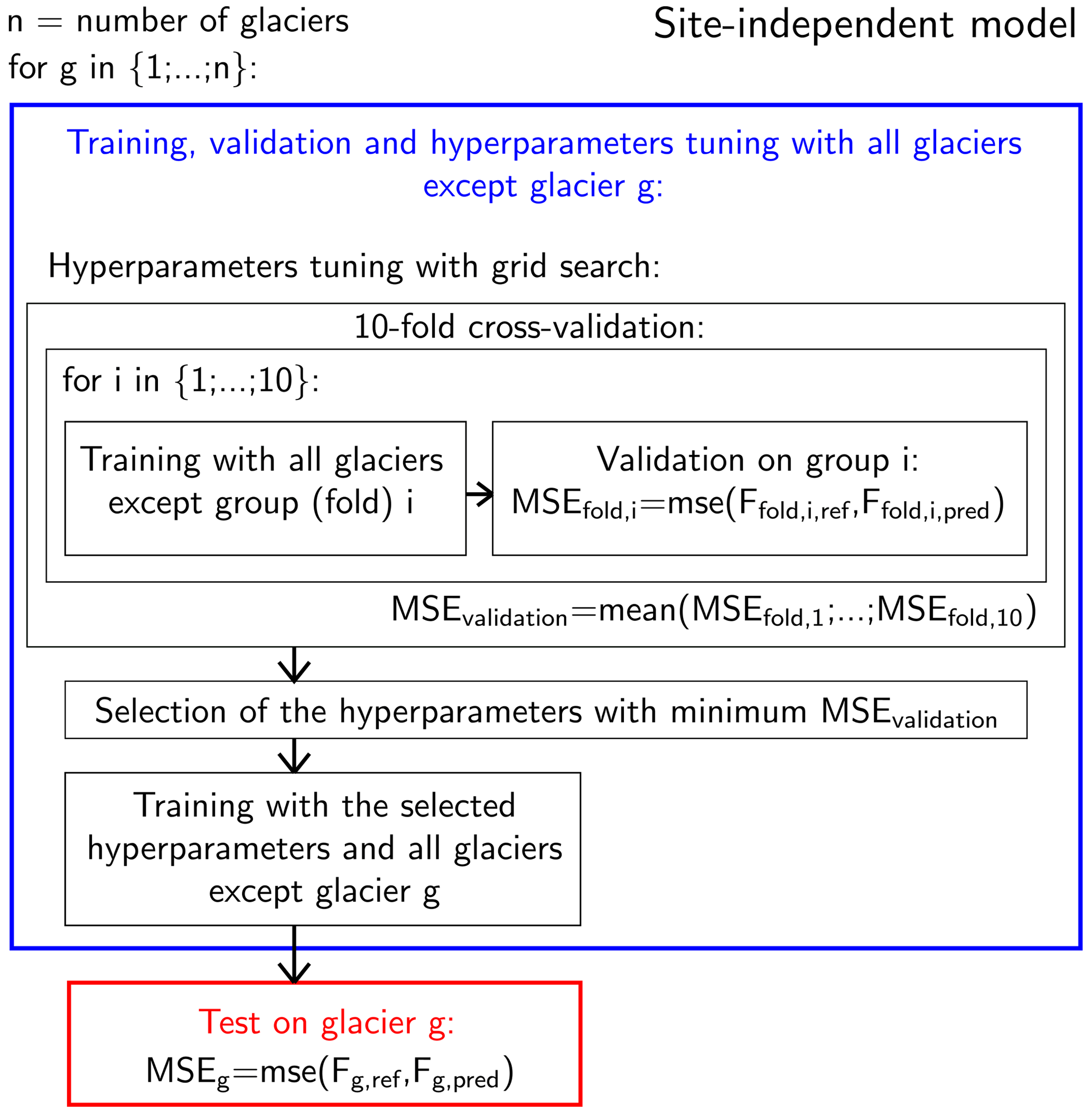
Figure 2Training, cross-validation with hyperparameter selection and test scheme for the site-independent GBR model. FdB, ref is the reference adjustment factor (Eq. 2), and FdB, pred is the adjustment factor predicted by the GBR model.
The second GBR model is season-independent and aims at extrapolating the Bw data in time only (filling data gaps over glaciers with discontinuous records of Bw). For the season-independent GBR, we built a model for each year (when the Bw data are available) and each glacier. In this case, each year of each glacier is used, in turn, as an independent test for the GBR, which is trained using the data of the other years (of the tested glacier) and of the other 94 glaciers. Thus, unlike the site-independent GBR, the season-independent GBR is informed with data of the glacier where the model is tested, excluding only data of the year when the model is tested. For the season-independent GBR, data of the other 94 glaciers are still used in the training, because many glaciers only have a small number of years with available Bw data. Thus, in the case of limited Bw data, this may help the GBR to learn from the data of the other 94 glaciers.
Table 1Average hyperparameters of the optimized GBR models of all the studied glaciers: “n estimators” is the number of additive trees (i.e. iterations) in the GBR, “max depth” is the maximum depth that each tree can reach, “min sample leaf” is the minimum number of samples required to be at a leaf node of a tree, “learning rate” determines how quickly the GBR learns (it shrinks the contribution of the individual trees on the GBR prediction) and “subsample” indicates the fraction of samples used for fitting the individual trees.
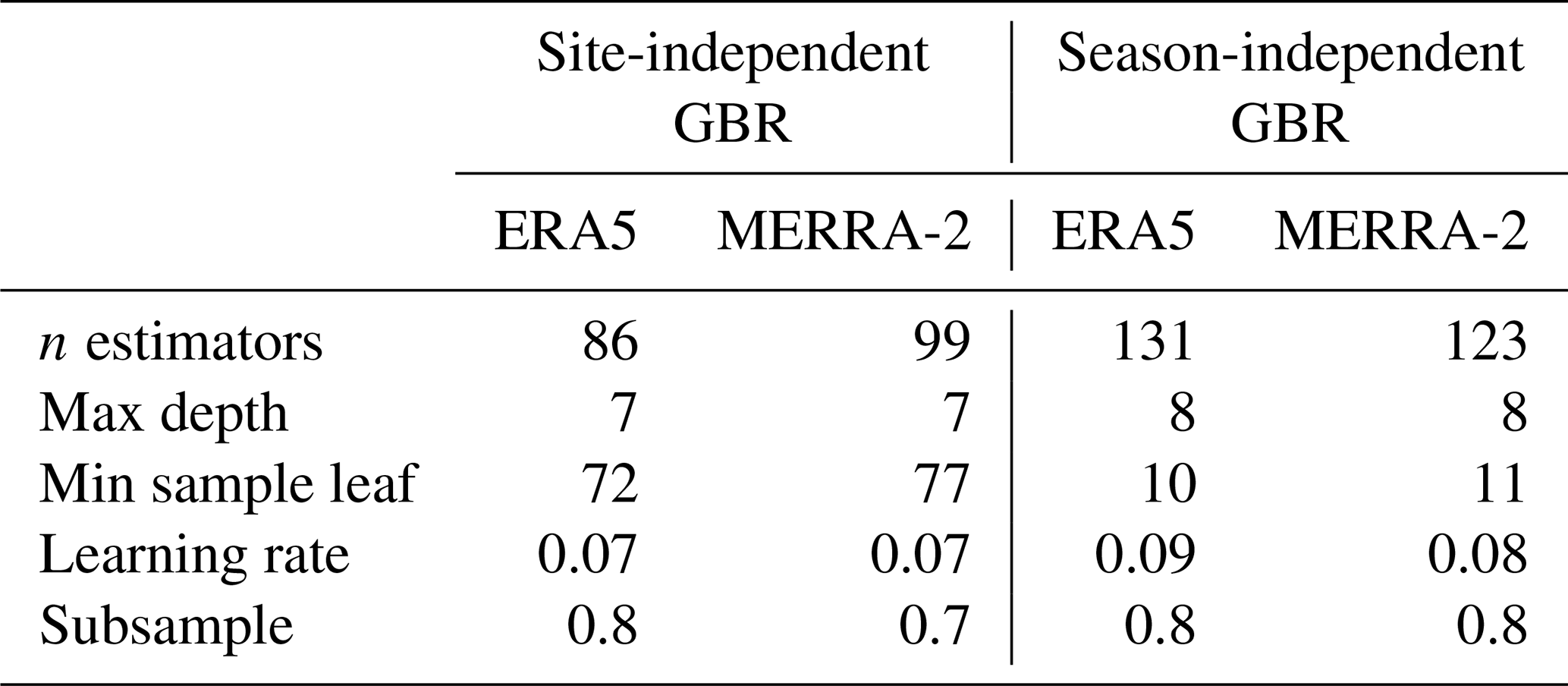
The average optimal hyperparameters for all the studied glaciers are reported in Table 1. The resulting site-independent model is more generalized (smaller number of estimators than the season-independent GBR and higher minimum number of samples per leaf), while the season-independent model is more detailed and can be split into individual sub-models adapted to a small number of samples. The different architecture between the site-independent and the season-independent GBRs is discussed in Sect. 5.2.1.
All variables presented in Sect. 2.1 and listed in Sect. B of the Appendix were considered by the GBR as predictors (separately for ERA5 and MERRA-2). In addition, we derived and used the differences between the downscaled variables (cf. Sect. 3.1) and the estimates at the grid of the reanalysis. Some variables were not only averaged considering all days in the accumulation season but also considering only the days with a relevant amount of precipitation, here arbitrarily set to 5 mm. The GBRs also use the latitude and longitude of the glacier (same value for the entire glacier), as well as aspect and slope of the glacier (same value for the entire glacier). A summary of the predictors used by the GBRs is provided in Table B3.
During the training phase of our models, the Bw data were weighted by considering the area of the glacier related to the respective elevation interval. Larger glaciers (and elevation intervals related to larger areas) thus receive more weight than smaller glaciers (and elevation intervals related to smaller areas).
3.3 Evaluation metrics for the models' estimates
3.3.1 Adjustment factors
In order to evaluate the bias between the Bw data and the estimates of the models (original reanalyses, benchmark or GBR), we computed the adjustment factor f (dimensionless) as
where Emodel is the estimate of a model. The adjustment factor FdB is expressed in decibels and is used to derive supplementary evaluation metrics:
3.3.2 Glacier-wide means
When deriving a glacier-wide factor (or glacier-wide Bw) for a single accumulation season, we computed a weighted mean of the area contained in the individual elevation intervals. These seasonal glacier-wide values were used to derive Pearson's correlations (r), the root mean square error (RMSE) and the fraction of standard error (FSE) between the glacier-wide Bw and the model estimate. The FSE corresponds to the RMSE divided by the glacier-wide Bw.
3.3.3 Regional metrics
In order to further validate the performance of the GBR models, we derived the glacier-wide FdB described by Eq. (5) for every accumulation season and every glacier with Bw data (FdB, mean). We thus analysed the four investigated regions separately by deriving a mean factor per region as
where n is the number of glaciers, and mg is the number of accumulation seasons with Bw data for the glacier g.
In the following, we first present the main results of our study, i.e. the performance of the GBR models over glaciers in the Alps, Scandinavia, Central Asia and western Canada (Sect. 4.1), followed by the analysis of the predictors' importance in the GBR models (Sect. 4.2).
4.1 Performance of the GBR models
Overall, the GBR models indicate better agreement in terms of bias and spatial and temporal correlation with the Bw data than the original reanalyses and the benchmark for the majority of the studied glaciers. In the following we report in detail on the comparison between the Bw data, the precipitation estimates of the reanalyses and the GBR models' estimates.
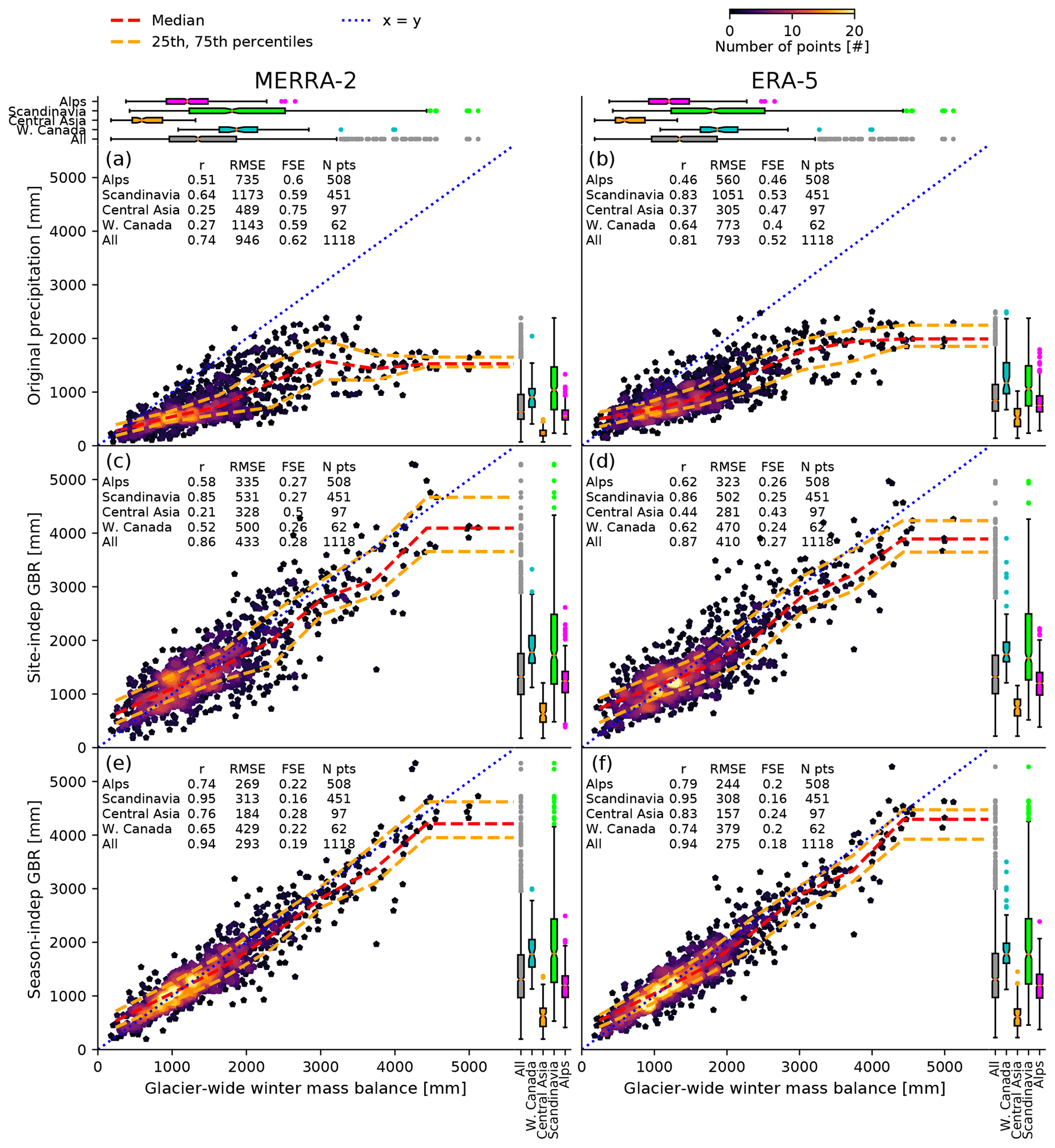
Figure 3Comparison between all glacier-wide Bw values and the model estimates: (a) original MERRA-2, (b) original ERA5, (c) MERRA-2 site-independent GBR, (d) ERA5 site-independent GBR, (e) MERRA-2 season-independent GBR and (f) ERA5 season-independent GBR. The Pearson correlation (CORR), the root mean square error (RMSE), the fraction of standard error (FSE, corresponding to the RMSE divided by the regional mean Bw) and the number of all seasons of all glaciers (N points) for each region are also reported. The boxplots indicate the distribution of the model's estimates (right) and of the Bw data (top) for each region.
4.1.1 Glacier-wide reanalysis' bias adjustment
Figure 3 shows the comparison between all glacier-wide Bw values and the models' estimates. MERRA-2 precipitation underestimates Bw more importantly than ERA5 precipitation in all regions (Fig. 3a and b), with an overall RMSE of 946 mm (mean absolute error (MAE) of 749 mm) against 793 mm (611 mm) of ERA5. Excluding the Alps, the correlation between the Bw data and the ERA5 precipitation is always higher than the correlation with the MERRA-2 precipitation. The adjusted estimates obtained with the site-independent and the season-independent GBRs allowed us to consistently reduce (increase) the bias (Pearson correlation (r)) between the precipitation of the original reanalyses and Bw (overall RMSE of 433 mm, MAE of 326 mm, r of 0.86 for the MERRA-2 site-independent GBR; RMSE of 410 mm, MAE of 307 mm, r of 0.87 for the ERA5 site-independent GBR; RMSE of 293 mm, MAE of 211 mm, r of 0.94 for the MERRA-2 season-independent GBR; RMSE of 275 mm, MAE of 200 mm, r of 0.94 for the ERA5 season-independent GBR). These results demonstrate the need of an adjustment of reanalyses data to reproduce Bw data on glaciers, which are, otherwise, largely underestimated in all four regions involved in this study.
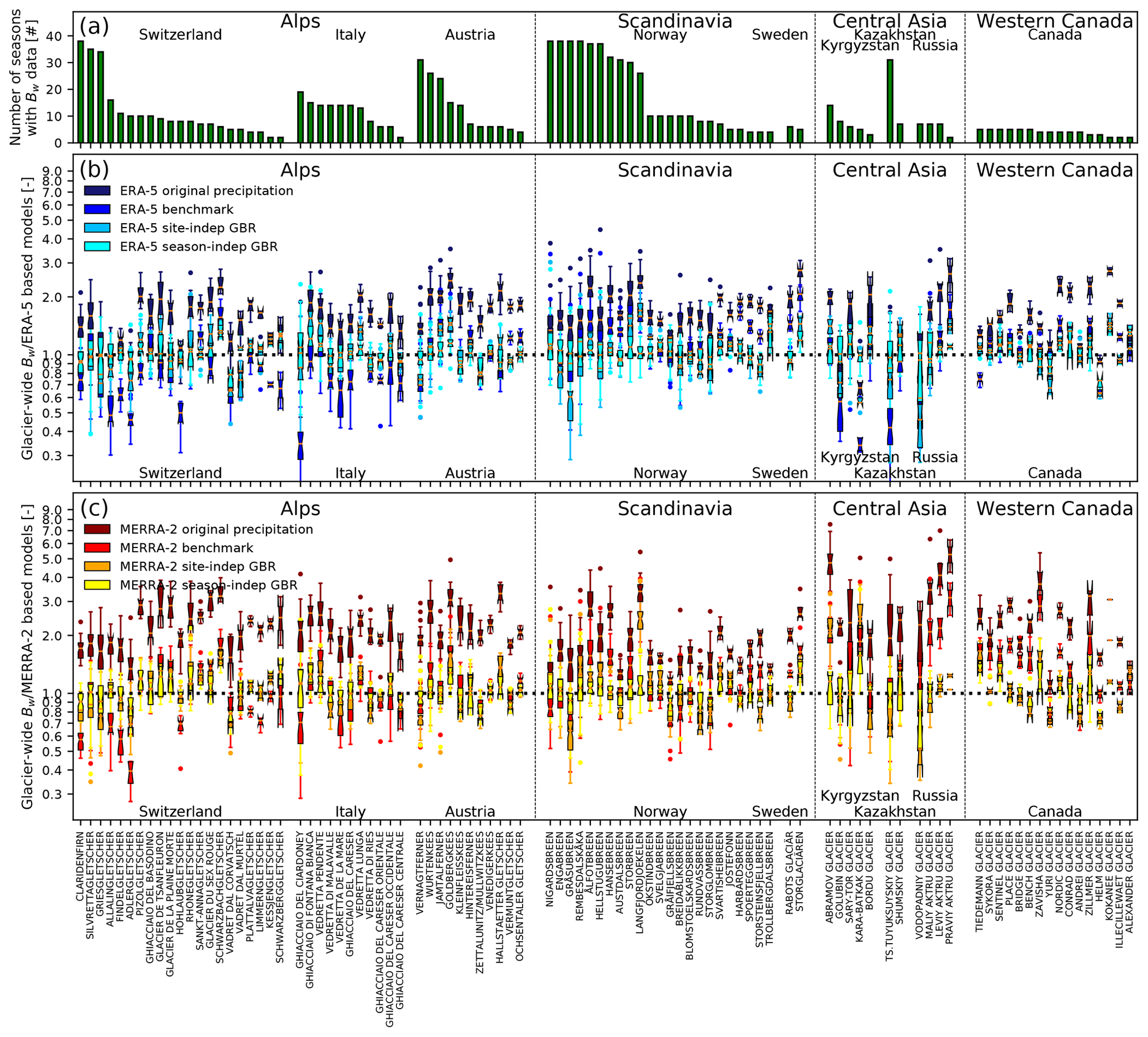
Figure 4(a) Number of seasons with available Bw data for each glacier. Factors between seasonal glacier-wide Bw and (b) ERA5-based models and (c) MERRA-2 based models, for each glacier of the study. The variability shown in the boxplots is given by the different seasons of Bw data.
In order to make an in-depth analysis of the model performance, we also derived a glacier-wide factor between the Bw data and reanalysis-based models' estimates (Eq. 4) for each accumulation season and for each site separately (Fig. 4). By comparing Fig. 4b and c, it is clear that, in Central Asia, the factors for adjusting the MERRA-2 reanalysis' precipitation are much larger than the factors for the ERA5 precipitation. The benchmark method overestimates the Bw for many glaciers in the Alps (both ERA5 and MERRA-2) and several glaciers in Central Asia (ERA5). The site-independent and, especially, the season-independent GBRs are better scaled with respect to the Bw data than the original reanalyses and the benchmarks. In general, the variability of the factors for each glacier is strongly affected by the number of available accumulation seasons with Bw data (Fig. 4a). A lower variability is usually observed for glaciers with a small number of seasons with Bw data.
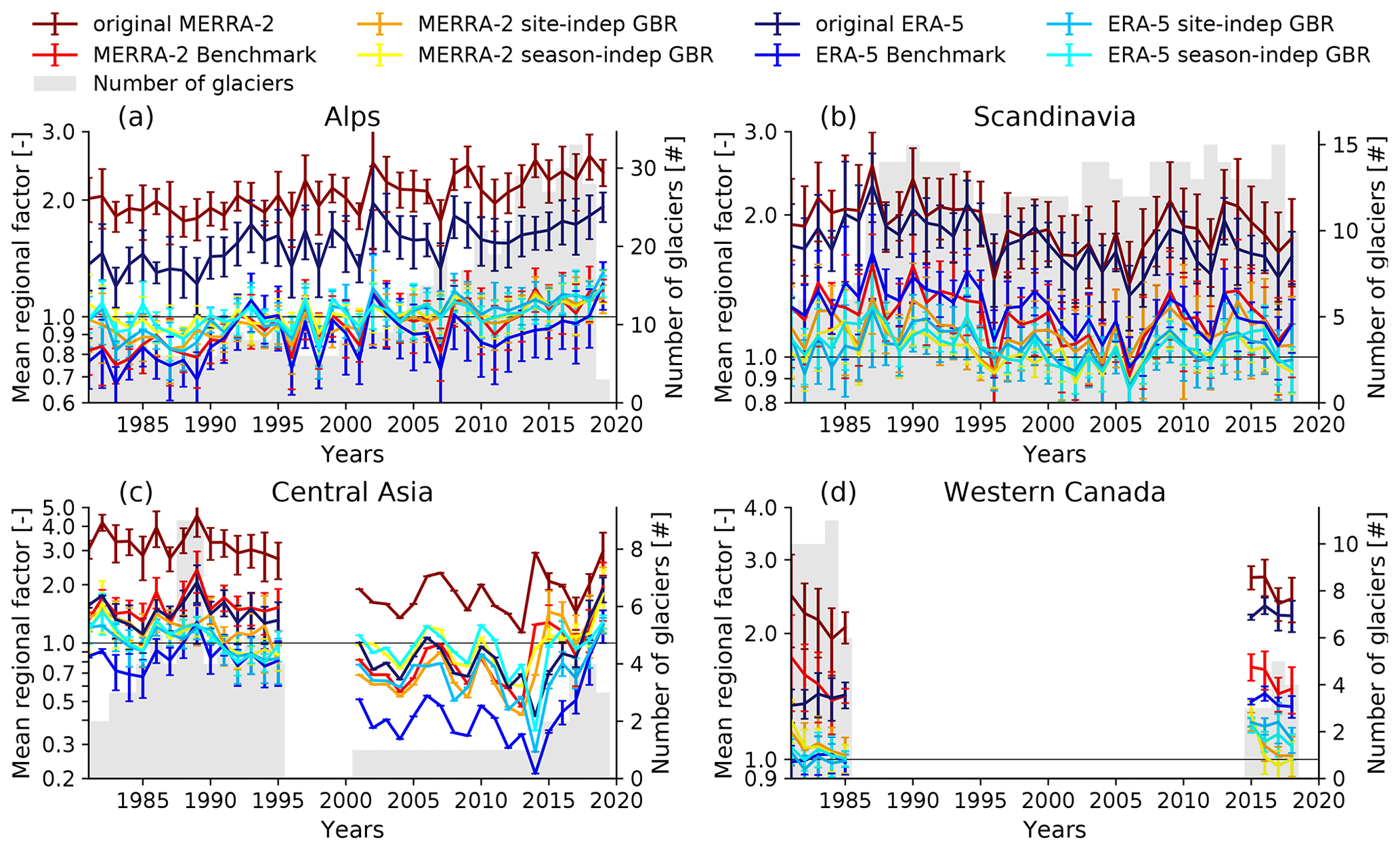
Figure 5Mean regional factor between the Bw data and the reanalysis-based models' estimates as a function of the accumulation seasons from 1981 to 2019 (last available season): (a) the Alps, (b) Scandinavia, (c) Central Asia and (d) western Canada. The error bars indicate the standard deviation of the regional factors. For each season, all glaciers with available Bw data were considered (the number of glaciers used to derive the regional factor is indicated by the grey bars).
Figure 5 shows the mean regional factor between the Bw data and the models' estimates as a function of the accumulation seasons from 1981 to 2019. It indicates that the original reanalyses clearly underestimate Bw on glaciers, except for ERA5 in Central Asia, where, as a consequence, the benchmark overestimates Bw. However, temporal variations in the mean regional bias are also affected by the considered set of glaciers that fluctuates over the analysed years. In the Alps, we observe increasing biases of the original reanalyses in recent years, where a much larger number of glaciers is available. In Scandinavia, the bias of MERRA-2 and ERA5 is similar and all the models are generally not able to remove it completely. In Central Asia, there is a tendency for all models to yield lower adjustment factors before the 2000s than afterwards. However, this has to be interpreted with care, because only one glacier was considered between 2002 and 2014. The continuity of the available Bw data in western Canada is too limited to analyse temporal changes in the adjustment factors.
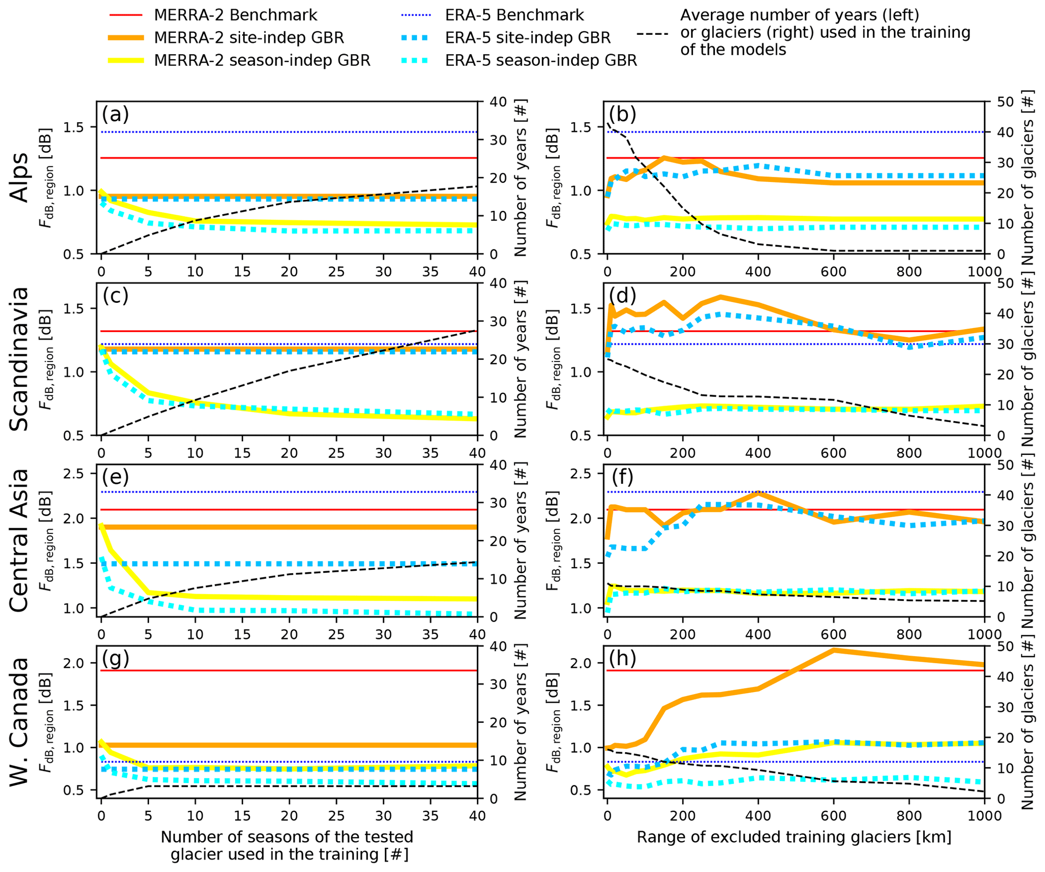
Figure 6Evaluation of the mean regional factor between the Bw data and the reanalysis-based models' estimates (FdB, region defined in Eq. 6) depending on different data used in the training of the GBR models. (a, c, e, g) Evaluation of the performance of the season-independent GBR models as a function of the number of seasons of the tested glacier used in the training (from no data to a maximum of 40 years of data of the tested glacier). (a) Model validation depending on the number of training seasons per glacier in the Alps, (c) Scandinavia, (e) Central Asia and (g) western Canada. (b, d, f, h) Evaluation of the robustness of the GBR models as a function of the number of other glaciers in the same region used in the training. All glaciers located within a range growing from 0 to 1000 km from the tested glacier were excluded from the training. (b) Model evaluation depending on the range of excluded glaciers from the training in the Alps, (d) Scandinavia, (f) Central Asia and (h) western Canada.
In order to evaluate the robustness of the GBR models to reduce the glacier-wide bias of the reanalysis, we performed a temporal and spatial validation of their predictions (Fig. 6). The performance of the season-independent models improves when using more accumulation seasons in the training data (Fig. 6a, c, e and g). Training the models with more than 20 seasons, however, does not seem to further improve performance consistently. The performance of the site-independent models is constant, because they are never trained with Bw data of the tested glacier. When no Bw data of the tested glacier are used to train the season-independent models (as for the site-independent models), their performance is worse than the site-independent models, confirming the importance of a specific optimization scheme depending on the goal of the model.
As also expected, the performance of the site-independent models decreases when data of neighbouring glaciers are excluded from the training (Fig. 6b, d, f and h). The highest impact is on the performance of the MERRA-2 site-independent GBR in Central Asia. Overall, the bias of the site-independent GBR models remains comparable to the bias obtained with the benchmark method even when excluding all other glaciers located within 1000 km from the training. For the season-independent models, we always kept the Bw data of the tested glacier in the training data and only excluded the other glaciers. This explains why the season-independent models perform better and are less sensitive to the removal of neighbouring glaciers from the training process.
The good performance of the GBRs in terms of bias suggests that they can be used for Bw reconstruction over glaciers where no ground observations are available (site-independent GBRs) and for filling data gaps of the recorded observations (season-independent GBRs). However, the performance generally decreases when the glacier is not in proximity to the glaciers used to train the GBR models. Furthermore, we assume that the resulting performance strongly depends on the characteristics of the glacier with respect to the glaciers used in the training. The results indicate moreover that the season-independent GBRs outperform the site-independent GBRs to reduce the bias against Bw data, especially in regions with a limited number of glaciers with Bw data. In conclusion, filling data gaps is much simpler than estimating Bw on glaciers with no observations.
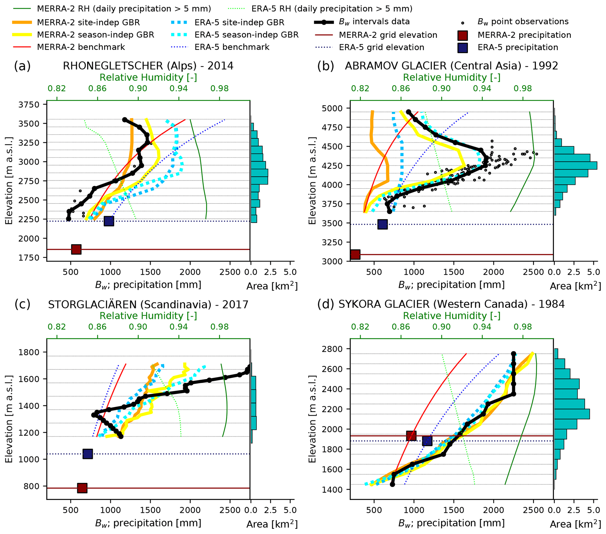
Figure 7Vertical profiles of Bw at the end of a specific accumulation season: (a) Rhonegletscher (Alps), (b) Abramov glacier (Central Asia), (c) Storglaciären (Scandinavia) and (d) Sykora glacier (western Canada). RH refers to the average relative humidity during days with a minimum precipitation of 5 mm. Note that the scale of the y axis differs between the panels.
4.1.2 Spatial winter mass balance variability on individual glaciers
In order to evaluate the ability of the GBR models to reproduce the spatial variability of the Bw over individual glaciers, we compared the vertical profiles of Bw to the estimates of the models. For Rhonegletscher for instance (Alps, Fig. 7a), both site-independent and season-independent GBRs are able to represent the shape of the vertical profile of the Bw, which is characterized by an increasing Bw until 3350 m a.s.l. and a more stable/decreasing Bw in the upper part of the glacier. This vertical profile cannot be reproduced by using the benchmark approach, where, by definition, the precipitation is monotonically increasing with the elevation. Decreasing Bw is also clearly indicated in the upper part of the Abramov glacier (Central Asia, Fig. 7b) in 1992. As suggested by the point observations reported, this is certainly the result of extrapolating to elevation ranges not or only poorly covered with data. However, this has a limited influence on the GBR models than the lower part of the glacier, as it received higher weights because of the larger areas (see Sect. 2.2). The site-independent GBRs are not able to adjust the precipitation by consistently reducing the bias with Bw. On the other hand, the season-independent GBRs are able to better fit the altitudinal distribution of Bw. In this case, we observe that the maximum Bw coincides with the maximum downscaled MERRA-2 relative humidity. In the case of Storglaciären (Scandinavia, Fig. 7c), Bw is underestimated by the benchmark, while the GBR models (the season-independent especially) are able to better represent the steep increase of Bw over the glacier. In the case of the Sykora glacier (western Canada, Fig. 7d), all GBR models show a good agreement with Bw data. By comparing the coefficients of variation, it is clear that the season-independent GBRs are able to better reproduce the amplitude of the spatial variability of the Bw than the site-independent GBRs (see Table S1 in the Supplement). Furthermore, the correlations demonstrate that the GBRs outperform the benchmark method to reproduce the Bw of almost all glaciers of this study (Table S1).
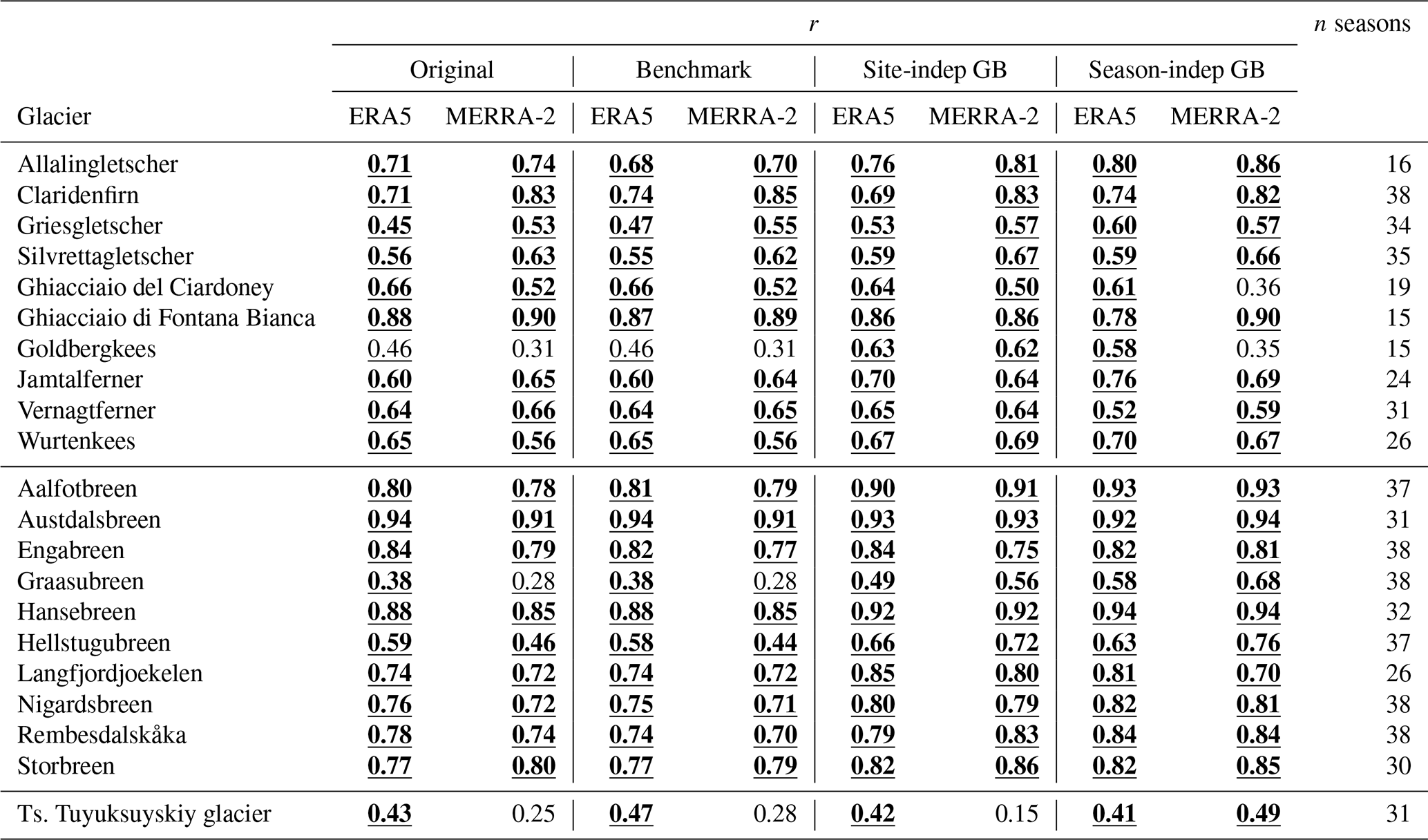
Table 2Pearson correlation (r [–]) between the reanalysis-based models and the glacier-wide Bw over the accumulation seasons (temporal correlation) separated by regions. Only the glaciers with a minimum of 15 seasons with Bw data are shown (i.e. no glacier in western Canada). The significance of the correlation is based on Student's t distribution. The level of the correlation significance is indicated as follows: normal font, not significant (p value >0.10); underlined, significant (p value ≤0.10); and underlined and bold, highly significant (p value ≤ 0.05).
4.1.3 Temporal winter mass balance variability on individual glaciers
In general, the GBR models show a better performance in reproducing the relative changes of Bw among individual years for the same glacier than the original reanalysis (see Table 2). The correlation between the GBR models' estimates and the Bw over the years is often much higher than for the original reanalysis. The level of significance of the correlation between the original ERA5 and/or MERRA-2 improves when the GBR models are applied, especially for Goldbergkees, Graasubreen and the Ts. Tuyuksuyskiy glacier. However, in some cases we still have low correlations, indicating that the models are not suitable to represent the temporal variability. Furthermore, although the season-independent GBRs are the best models to reduce the bias, the relative changes among years are sometimes better explained by the site-independent GBRs. In fact, the number of years of data of the tested glacier used to train the season-independent GBRs does not seem to impact its performance in terms of temporal correlation with the Bw data (see Fig. S3). The number of years with available Bw data is typically much smaller in western Canada and Central Asia than in the Alps and Scandinavia (see Fig. 4a); therefore, we could not robustly evaluate the ability of the models to represent the temporal variability of the Bw data for these regions.

Figure 8Overall root mean square error (RMSE) between Bw and GBR models using different groups of predictors, for all analysed glaciers and years: (a) ERA5 site-independent GBR, (b) MERRA-2 site-independent GBR, (c) ERA5 season-independent GBR and (d) MERRA-2 season-independent GBR. The “pressure-level” group refers to all variables derived from the pressure-level data, i.e. “downscaled” variables and “delta_variable” (except for the elevation difference) in Table B3. The “single-level” group refers to all single-level variables listed in Table B3. The “topography” group refers to the topographical parameters describing the reanalysis’s subgrid complexity (all constants in Tables B1 and B2) and the average slope and aspect of the glaciers by using the information provided in the Randolph Glacier Inventory version 6 (RGI Consortium, 2017).
4.2 Importance of predictors in the GBR models
In order to understand the importance of the predictors used by the GBR models (i.e. those not related to the elevation of the glaciers and their elevation difference with the reanalysis' grid), we evaluated the changes in terms of overall GBR model performance when suppressing groups of predictors. For both ERA5 and MERRA-2 site-independent GBR models, the smallest RMSE results when using all predictors (Fig. 8a and b). The RMSE particularly increases when suppressing the MERRA-2 single-level and pressure-level variables from the predictors. In turn, for both ERA5 and MERRA-2 season-independent GBR models, the smallest RMSE results when suppressing the single-level and pressure-level variables from the predictors (Fig. 8c and d). The RMSE increases most when suppressing the year, the topographical parameters and the glacier coordinates simultaneously as predictors.
However, skipping reanalysis variables from the set of predictors leads to higher errors for some individual glaciers, especially in the representation of the temporal variability of the Bw data. In fact, by excluding the reanalysis variables, the year is the only predictor able to vehiculate the climatological information; in other words, the year is the only predictor that could be used by the GBR to predict a different adjustment factor depending on the accumulation season (all the other predictors are constant in time). Therefore, and to allow a fairer comparison between site-independent and season-independent GBRs, in all our following analyses we always included all predictors.
In order to infer the importance of the predictors for the individual study regions, we built an individual GBR for each region. We furthermore performed a principal component analysis (PCA) considering the 10 predictors most frequently used by the GBRs for each region. In the Alps, lower factors between Bw and ERA5 precipitation result at lower latitudes, and the glaciers affected by 100 m westerly winds (negative u component of the wind speed) have generally higher factors than those affected by easterly winds (Fig. S2a). In Scandinavia, we notice a cluster of five glaciers with smaller ERA5 factors and higher downscaled temperatures during precipitation events (Fig. S2c). In Central Asia, the glaciers' aspect is the predictor that most clearly discriminates between high and low factors between Bw and both ERA5 and MERRA-2 precipitation. Glaciers with ∼ north-facing slopes show smaller ERA5 factors and ∼ east-facing slopes higher MERRA-2 factors (Fig. S2e and f). In western Canada, lower ERA5 factors correlate with larger precipitation amounts and lower elevation of the glaciers, while MERRA-2 factors are clearly lower at higher latitudes, which are characterized by stronger southerly winds at 850 hPa (Fig. S2g and f).
The GBR models developed, evaluated and presented in this study showed a better overall agreement in terms of bias and spatial and temporal correlation with the Bw data than the original reanalyses and the benchmark (lapse-rate-based approach described in Sect. 3.2.1) for the majority of the studied glaciers in the Alps, Scandinavia, Central Asia and western Canada. In the following, we provide a comprehensive discussion of the approach and the results.
5.1 Advantages and disadvantages of gradient boosting regressors
5.1.1 Differences with lapse-rate-based approaches
With the exception of some specific sites, our GBR models outperformed the benchmark method (lapse-rate-based approach (Sect. 3.2.1)) in the Alps, Scandinavia, Central Asia and western Canada regarding the reduction of the bias against glacier-wide Bw data (Figs. 4 and 5). This suggests that data-informed models such as our GBRs are needed to adjust reanalysis to different glacier sites, which can be characterized by different topographical and climatic conditions, and where the performance of reanalysis' estimates can vary greatly depending on the region (e.g. Sun et al., 2018). In fact, (independent) Bw data were used to train our GBR models, allowing the GBRs to learn specific characteristics of actual Bw on glaciers and to transfer them to unknown sites (site-independent GBRs) and unknown seasons (season-independent GBRs).
The GBR models also outperform the benchmark to reproduce the spatial variability of Bw on individual glaciers. We observed lower Bw in the uppermost sections of many glaciers, which may be attributed to preferential snow deposition redistribution processes, caused by the interplay between snow, wind and the generally steep topography (e.g. Sold et al., 2016; Gerber et al., 2019). The ability of GBRs to model non-linear relationships allows for a better representation of the vertical profiles of Bw than the benchmark method (Fig. 7, Table S1). In fact, the observed spatial variability of Bw could not be reproduced with the benchmark method, which by definition cannot represent decreasing values with the elevation (cf. Eq. 1).
Both the GBR models and the benchmark do not require direct in situ observations to be applied. However, the benchmark method is independent from any Bw data used in this study (not data-informed). In turn, the performance of the GBR models is influenced by the number of data used to train the models and strongly depends on the characteristics of the glacier with respect to the glaciers used to train the models.
5.1.2 Differences with other machine learning algorithms
Intuitively, we preferred a tree-based algorithm given the high inhomogeneity in terms of spatial distribution of the considered glaciers. As further discussed in Sect. 5.2.1, a tree-based algorithm can exploit the coordinates (if provided as predictors) to easily split into individual sub-models adapted to different regions of the world (from the continental scale to the glacier-specific scale). Such operations would not be possible by using a simpler model such as a multiple linear regression. Also, it is less clear to us how artificial neural networks would behave given the considerable inhomogeneity of the spatial distribution. In fact, we have chosen a tree-based algorithm because of its higher readability in terms of the predictors' usage compared to other machine learning methods (e.g. Huysmans et al., 2011; Freitas, 2014). A disadvantage of tree-based algorithms, however, could be that this approach does not predict continuous values. Yet, here, we aim at predicting an adjustment factor depending on a classification based on the used predictors, which is exactly the purpose of a tree-based algorithm. The choice of a gradient boosting instead of other tree-based algorithms (e.g. random forest; Breiman, 2001) is motivated by the fact that gradient boosting is a gradient descent algorithm, where each additional tree tries to reduce the bias (which is the main goal of our study) rather than the variance of the predictions.
5.2 Impact of the data used to train the GBR models
5.2.1 Site-independent and season-independent GBRs
The lower generalization of the season-independent GBRs compared with the site-independent GBRs allows for the splitting into individual sub-models adapted to a small number of samples (see Table 1). This enables us to exploit the Bw data of the tested glacier by creating a specific sub-model but can result in an overfit of the training data. On the contrary, the higher generalization of the site-independent GBRs allows for learning on overall relationships between the used predictors and the reference adjustment factors (Eq. 2).
The used training data and the selected hyperparameters also have a direct influence on the predictors needed by the GBR models to reduce the cost function (Eq. 3). In fact, the use of reanalysis variables (from single level and pressure levels) as predictors caused an increase of the overall RMSE of both ERA5 and MERRA-2 season-independent GBRs against the Bw data of all glaciers of the study (Fig. 8c and d). However, despite the high correlation of the downscaled reanalysis variables (cf. Sect. 3.1) with the elevation of the glaciers, their inclusion in the set of predictors for the training of the site-independent GBRs reduced the overall RMSE (Fig. 8a and b). This difference can be explained by the combined effect of using data of the tested glacier in the training of the season-independent GBRs and defining a small minimum number of samples required to create a leaf node of the GBR. In fact, the season-independent GBR can theoretically exploit the coordinates to split into individual sub-models adapted to individual glaciers. Therefore, the season-independent GBRs can learn the adjustment factors observed in the other accumulation seasons of the tested glacier and predict a similar adjustment factor for the tested accumulation season, with no need for learning overall relationships between the reanalysis predictors and the reference adjustment factors (Eq. 2).
In general, the year was included in the set of predictors for the GBRs, because it may allow for learning the climatological information and potential trends in terms of reanalysis biases against the Bw data. This can be relevant in case reanalysis variables included in the predictors are not able to represent the hypothetical trends of these biases, which can exist due to the increasing availability of observational data that could have been assimilated by reanalysis models over the years. From Fig. 8, we notice that the year has a different impact on the site-independent and the season-independent GBRs. For the site-independent GBR, the withdrawal of the year from the predictors leads to a smaller increase of the overall RMSE than the withdrawal of the reanalysis variables (pressure levels and single level). In contrast, for the season-independent GBR, the best performance is reached by withdrawing the reanalysis variables. Thus, given the mentioned ability of the season-independent GBR to potentially create sub-models for specific glaciers using their coordinates, we think that the year may be the one predictor to actually vehiculate the climatological information in this case (the GBR model learns which periods correspond to larger/smaller biases for the tested glacier).
5.2.2 Spatial and temporal transferability of the GBR models
The GBR models were trained with almost 100 glaciers distributed over the four regions on three continents. Between the regions we observed different robustness and performances. The performance of the GBR models tends to decrease when removing Bw data of neighbouring glaciers from the training process (Fig. 6b, d, f and h). Neighbouring glaciers were removed from the training as a function of the distance (range) from the tested glacier. Our results suggest that more available glaciers with Bw data would probably greatly improve the performance in Central Asia and western Canada, where our dataset is limited in terms of the number of monitored glaciers, and the horizontal spacing between different sites is considerable. In the Alps, the network of monitored glaciers is much denser. Thus, more glaciers are excluded from the training for shorter distances than in other regions, impacting the performance of the site-independent GBR models. When the range of excluded neighbouring glaciers is extended to 1000 km, a strongly reduced number of glaciers of the same region is still used in the training, meaning that the models are almost exclusively trained with the glaciers of the other regions (the site-independent GBR almost becomes a region-independent GBR). The climate conditions and the complexity of the weather processes can be very different among the four investigated regions (and even within the individual regions). A region-independent model is thus not expected to provide accurate results. In Scandinavia, a linear precipitation gradient with elevation is more appropriate than in the more complex topography of the Alps and Central Asia (e.g. Rasmussen and Andreassen, 2005). Thus, the site-independent GBR models are only performing slightly better than the benchmark when the full set of the other glaciers is used in the training, indicating that a simpler lapse-rate-based approach might be preferable. However, considering the four regions, the bias of the region-independent GBR models remains comparable to the bias obtained with the benchmark method, which is independent from any ground observation.
The performance of the season-independent GBR models improved consistently when including in the training only a few other seasons of Bw data related to the tested glacier (Fig. 6a, c, e and g). This thus demonstrates the uniqueness of the Bw distribution over each glacier that cannot be easily reproduced by using the relations learned at other glaciers. However, this also indicates that the Bw distribution, and its relation with precipitation, is similar in different years (see also e.g. Grünewald et al., 2013; Sold et al., 2016). For our application, there would be the added benefit from Bw data on additional glaciers rather than on additional seasons.
The inclusion of the year in the set of predictors is not problematic for temporal reconstruction of Bw with limited gaps but could be a limitation for extrapolation to future conditions (using for instance global or regional climate model data in lieu of reanalysis). In fact, even though the use of the year as predictor could allow for identifying and modelling trends of reanalysis biases against the Bw data, these trends would be limited to the training period of the GBRs. In contrast, the exclusive use of reanalysis variables as predictors could allow for identifying and modelling trends of biases as a function of specific climatological conditions represented by reanalysis variables.
Furthermore, the use of total seasonal averages as inputs for the GBRs has limitations for the application of the presented approach. The GBRs provide an estimate of the overall adjustment factor for the reanalysis precipitation according to the average climatic conditions of the accumulation season. Thus, a unique adjustment factor is estimated for the whole accumulation season. The application of this adjustment factor to daily precipitation data would allow for obtaining an average estimate of the SWE evolution during the accumulation season. However, the obtained SWE evolution would neglect potential melt of snow during the accumulation season (see Sect. 2.2), as well as potentially different adjustment factors for precipitation at higher temporal scales than seasonal. This limitation is related to the lack of reference in situ observations at higher temporal resolution than seasonal available for our study, focusing on different regions of the world and at high elevations.
5.2.3 Representation of the temporal variability of the winter mass balance
All GBRs aimed at minimizing the MSE between the predicted and reference logarithmic adjustment factors (Eq. 3). The improvement of the temporal correlation between the original reanalysis and the Bw data is thus a consequence of bias-adjusted estimates over accumulation seasons rather than a primary goal of the GBRs. A sensitivity test reported in the Supplement (Fig. S3) suggests that the season-independent GBRs are not very sensitive to the number of years of data of the tested glacier used for training. Their performance is comparable to the site-independent GBRs (Table 2). Furthermore, only in a few cases did the site-independent GBRs show a performance inferior to the original reanalysis or the benchmark method (e.g. Ts. Tuyuksuyskiy glacier). These promising results suggest that our new estimates could also be used to derive Bw trends with generally higher accuracy than the original reanalyses, thus potentially providing insights into the relation between climate change and both snow accumulation and precipitation at the highest elevations of mountain ranges, where virtually no direct precipitation records are available. Still, the limited number of glaciers with abundant Bw data coverage available over a sufficient number of years does not allow us to perform a complete application of this approach.
5.2.4 Impact of the chosen reanalyses on the GBR models
At a regional scale, the total precipitation estimated in the accumulation season by the original MERRA-2 has shown larger biases than the original ERA5 when compared to Bw on glaciers. The coarser spatial resolution of MERRA-2 is certainly a factor causing larger biases in complex high-mountain areas (e.g. Zandler et al., 2019; Chen et al., 2021). In fact, a coarse resolution directly implies that mountains are more strongly smoothed. The absolute elevation of a grid cell is thus lower for a coarse resolution, and the estimated precipitation also refers to the lower elevation of the grid cell.
The performance of the original ERA5 and MERRA-2 has a direct impact on the GBR models. However, the GBR models were able to compensate for such differences in the bias. In fact, the biases of the ERA5 and MERRA-2 GBR models are much closer to each other than the biases of the original reanalyses (see Fig. 3a–d). The differences between the performance of our GBR models are also caused by the different predictors that have been used. For instance, we considered all the topographical predictors describing the reanalysis’s subgrid complexity of both reanalysis products, and ERA5 is providing more descriptors than MERRA-2 (see Tables B1 and B2).
5.2.5 Influence of the winter mass balance data accuracy on the GBR models
Our study strongly relies on reference Bw data on glaciers. However, various problems are related to the direct measurements of snow accumulation on glaciers thus leading to uncertainties in the observations (e.g. Zemp et al., 2013; Sold et al., 2016; O'Neel et al., 2019; Huss et al., 2021). Most importantly, snow accumulation measured at individual points needs to be extrapolated in space to obtain Bw data used in our analysis. At the highest elevations of glaciers with a typically difficult accessibility for manual observations, results are often purely based on extrapolation techniques (e.g. Østrem and Brugman, 1991; Cogley et al., 2011; Huss et al., 2021). Given that the WGMS database does not generally report how this was achieved and how many actual observations were available in a given elevation interval, it is difficult to assess the integrative uncertainty in the Bw data used. In order to illustrate the importance of the extrapolated Bw data used in this study, we more closely inspected point winter snow observations for 12 Swiss sites and three years (2016–2018) based on a dataset with higher resolution and full documentation (GLAMOS, 2021).
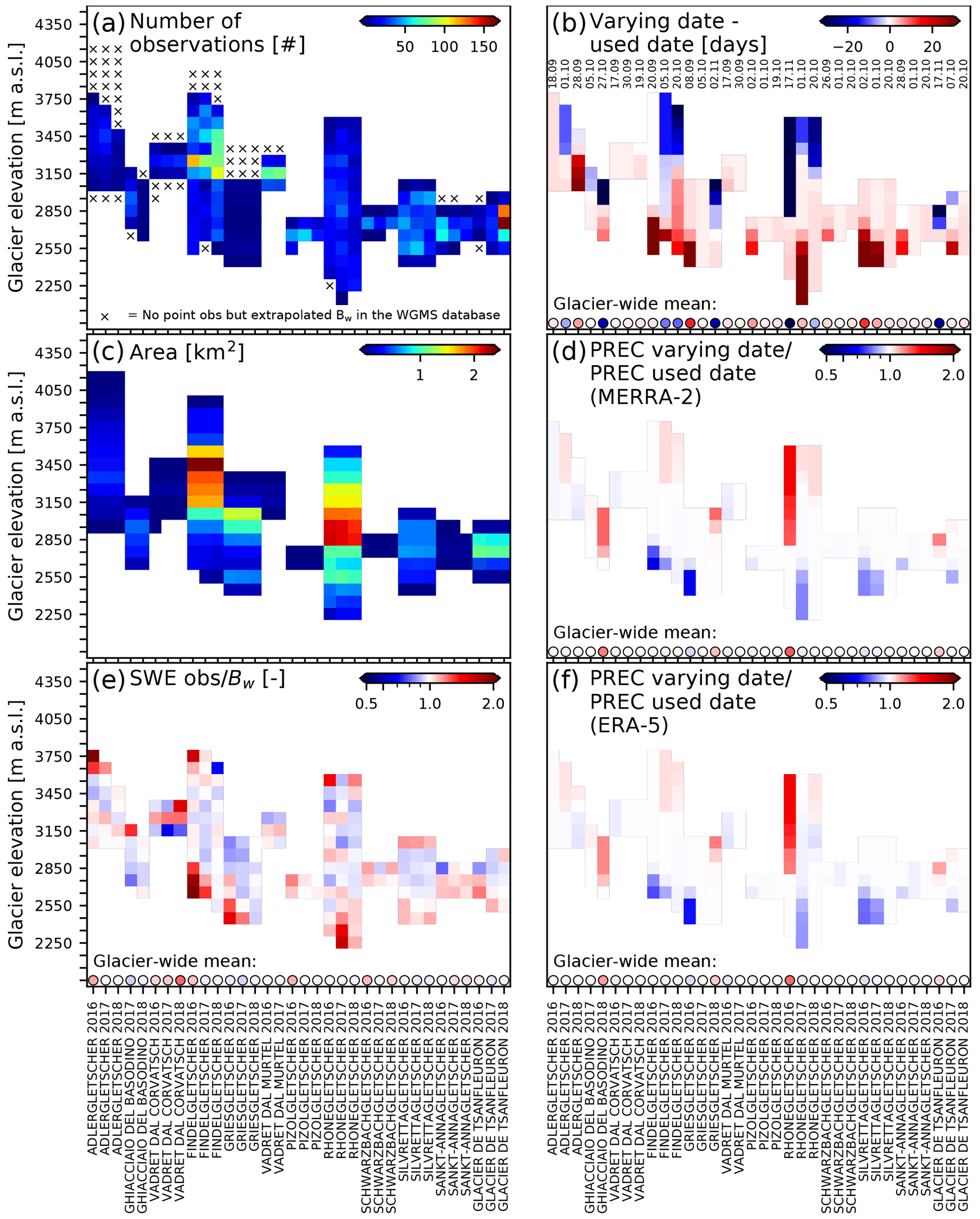
Figure 9Sensitivity analysis of extrapolated Bw data and used starting dates for 12 glaciers in the Swiss Alps between 2016 and 2018 (GLAMOS, 2021). (a, c, e) Difference between Bw data used in this study and point-SWE observations: (a) number of manual observations performed in the elevation intervals of the glaciers. (c) Area of the glacier according to the elevation interval. (e) Ratio between the observed SWE and the Bw data. (b, d, f) Impact of the date considered the beginning of the accumulation season on seasonal precipitation totals: (b) differences between accurate (varying) dates of the beginning of the accumulation period and the used dates in the study (the day and the month of the used dates are written on the figure (DD.MM)). (d) Ratio between the total precipitation of MERRA-2 according to the accurate dates and the used dates. (f) Ratio between the total precipitation of ERA5 according to the accurate dates and the used dates.
Figure 9a indicates that a lower number of manual observations was typically performed at the lowest and the highest elevations of the glaciers. In some elevation bands, even no manual observations are available and Bw data refer to an extrapolation. However, a much larger number of manual observations is typically performed in the elevation intervals corresponding to the largest areas of the glaciers (Fig. 9a and c). As indicated by Fig. 9e, considerable uncertainties might exist in the analysed vertical profiles of Bw. However, the weighting function dependent on the area of the intervals used in the training of the GBR models assigned more importance to the Bw data in such observation-rich areas. Furthermore, the main results of the study relate to glacier-wide Bw data, which for most glaciers is very close to the glacier-wide mean of the manual observations as also indicated in Fig. 9e (only in 3 out of 34 cases is the ratio of glacier-wide mass balance to the average of all individual observations larger than 1.10, and in no case is the ratio lower than 0.90).
Another source of uncertainty that is difficult to assess is the starting date of the accumulation season. We considered the same starting date for all elevation intervals, even though it varies over the glacier's elevation range. The accumulation of snow starts later at low elevations and earlier at high elevations. Therefore, the different elevations also collect different precipitation totals (as the periods differ). The impact on the study of the date considered the beginning of the accumulation season has been evaluated with a sensitivity test (Fig. 9). For the same 12 Swiss glaciers and 3 years as above, we rely on the more detailed dataset of point winter mass balance data that documents start dates of measured cumulative snow precipitation of the winter season for each location individually. Start dates have been inferred based on a distributed glaciological modelling approach driven by daily local weather data (Huss et al., 2021). The total precipitation of ERA5 and MERRA-2 was derived over these varying starting dates and was compared with the total precipitation obtained with non-varying, average starting dates (Fig. 9b, d and f). Figure 9b indicates that at high (low) elevations, the accumulation season can start up to 20 d before (after) the unique date that we considered for all elevation intervals. These differences may translate into different amounts of total precipitation. In extreme cases, the total MERRA-2 (Fig. 9d) or ERA5 (Fig. 9f) precipitation that would be obtained with varying dates would be almost twice (or half) of the total precipitation that we considered. However, the impact on the main results presented above is limited, because these large differences are typically observed at the highest/lowest elevations of the glaciers, where the glacier area is minor, and thus, a lower weight is assigned to the Bw data in the training of the GBR models. Moreover, the main results of the study are based on glacier-wide values, and for both MERRA-2 and ERA5 we observe very small differences in terms of glacier-wide precipitation totals for the majority of the Swiss glaciers. Only in 6 out of 34 cases is the glacier-wide ratio smaller (larger) than 0.97 (1.03), and only in two cases it exceeds 1.10.
This analysis suggests that the used Bw data and the considered start dates can lead to relevant uncertainties in the analysis of vertical profiles. However, this does not generally have a relevant impact on our conclusions, which are mainly based on glacier-wide values.
In this study, we developed and evaluated a machine learning approach based on gradient boosting regressor models to adjust the total precipitation of reanalysis datasets (ERA5 and MERRA-2) over the accumulation season on glaciers and to ultimately reconstruct spatio-temporal winter mass balance (Bw). The high performance achieved with our approach allowed us to use it to derive observation-independent Bw estimates over glaciers in the Alps, Scandinavia, Central Asia and western Canada. Data on Bw covering a period of up to 39 years from 95 glaciers (WGMS, 2021) were used to train our approach.
The most important variables that were automatically selected by our GBR models were those related to the elevation difference between the glacier surface and the terrain model underlying the reanalyses. The latitude and longitude of the studied sites were also frequently used in order to discriminate between regions that are characterized by different climate conditions and weather systems, allowing the GBR models to be split into individual sub-models adapted to specific sub-regions.
In general, the total precipitation of the reanalyses largely underestimates observed Bw on glaciers. The largest (relative) regional underestimation is observed in Central Asia for MERRA-2 and in Scandinavia for ERA5 (Fig. 3). The GBR models allowed for reducing these biases. In Central Asia and western Canada, the correlation between the original reanalyses' estimates and the Bw on the analysed glaciers has considerably increased with the season-independent GBRs only. With the exception of some specific glaciers, our GBR models outperformed the benchmark method (lapse-rate-based approach) in the Alps, Scandinavia, Central Asia and western Canada by reducing the bias of the original reanalysis against the Bw data (Fig. 4). This suggests that more complex and data-informed models such as our GBRs are needed to adjust reanalysis data to different glaciers located in different topographical settings and climatic conditions and to overcome the varying performance of reanalysis data for different region of the world.
Our results furthermore indicate that the season-independent GBRs outperform the site-independent GBRs to reduce the bias, which consequently makes filling temporal data gaps much simpler than estimating Bw of glaciers where no in situ observations are available. Thus, a denser network of ground-based snow accumulation measurements and/or improved remote sensing observations are of great importance to further develop methods that allow spatio-temporal transferability of the observed snow and/or precipitation in high-mountain areas.
The GBR models, compared to the original reanalyses, have moreover shown improved performance in reproducing temporal changes (over years) of Bw for the majority of the analysed glaciers. Generally, our GBR models would allow for deriving more accurate Bw trends than the original reanalyses, thus potentially providing insights on the relation between climate change and snow accumulation over glaciers.
We finally demonstrated that machine learning models (with robust cross-validation schemes) can be powerful instruments to adjust precipitation estimates over glaciers. The new information that our approach is able to deliver can significantly improve the calibration of glaciological and hydrological models in different regions of the world, in particular for regions where the quantity and quality of observations are very limited, and the spatial resolution and performance of reanalysis products are (too) low.
The relative humidity is not directly provided by all the reanalysis products; therefore we derived it by applying a similar approach to Liston and Elder (2006) and Gupta and Tarboton (2016), which is presented hereafter.
A1 ERA5
The relative humidity is not directly provided at the grid level; therefore, we combined the 2 m temperature (t2m) and dew point temperature (d2m) as follows:
where r2m* is the computed 2 m relative humidity, and for ice/snow, a=611.21 Pa, b=22.452 and c=272.55 ∘C.
A2 MERRA-2
MERRA-2 is not providing the relative humidity at the grid and at the pressure levels; furthermore, the dew point temperature is not provided at the pressure levels either. Therefore, we combined the specific humidity and the pressure in order to derive them (at the grid and at the pressure levels). For ice/snow, a=611.21 Pa, b=22.452 and c=272.55 ∘C.
Vapour pressure is
where the specific humidity is QV=QV10M for the grid and QV=QVlevels for the pressure levels, and the pressure is P=PS for the grid and P=Plevels for the pressure levels. The vapour pressure e* was named e10M* for the grid and for the pressure levels.
Dew point temperature is
The dew point temperature Td* was named Td10M* for the grid and for the pressure levels.
Relative humidity is
where the temperature is T=T10M for the grid and T=Tlevels for the pressure levels. The relative humidity RH* was named RH10M* for the grid and for the pressure levels.
In Tables B1 and B2, we report the complete list of variables selected from the reanalyses products. In Table B3 we provide a summary of all the variables used by the GBR models.
Table B1ERA5 variables used in the study.

* Ttp was used as precipitation variable.
Table B2MERRA-2 variables used in the study.
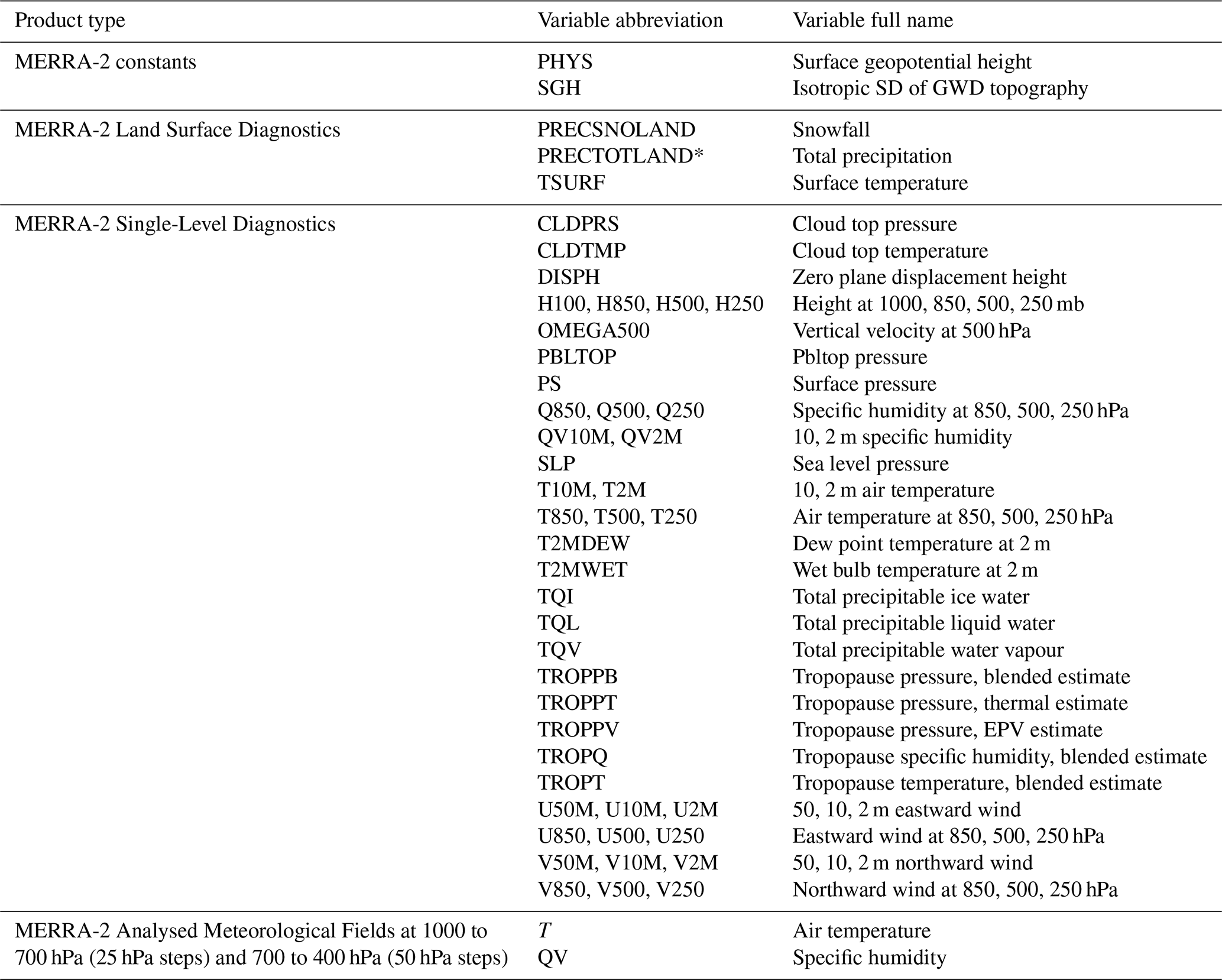
* PRECTOTLAND was used as precipitation variable.
Table B3Summary of the variables used by the GBR models: all constants and single-level variables from the original reanalyses (Tables B1 and B2), variables downscaled at the elevation of the Bw data (“variable_down”), mean of the variables during the accumulation season considering only days with a minimum precipitation of 5 mm (“variable_Ppos”), difference between “variable_down” and the variable at the original grid of the reanalysis (“delta_variable”), year, glacier coordinates, slope, and aspect. Pgrid is the precipitation of the original reanalysis. The variable names have the same roots as those reported in Tables B1 and B2.
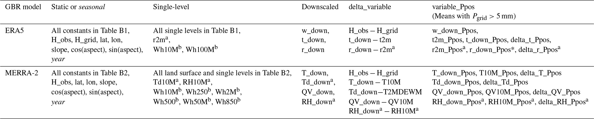
a These variables were derived using the equations reported in Sect. A. b These variables represent the wind speed derived with the two horizontal components.
Winter mass balance data separated per elevation interval are freely available at https://doi.org/10.5904/wgms-fog-2021-05 (EE-MASS-BALANCE data sheet in WGMS, 2021, last access: 1 June 2021). The average slope and aspect of the glaciers were obtained from the Randolph Glacier Inventory version 6 at https://doi.org/10.7265/4m1f-gd79 (last access: 5 May 2021, RGI Consortium, 2017). ERA5 hourly data on single levels and on pressure levels were downloaded from the Copernicus Climate Change Service (C3S) Climate Data Store at https://doi.org/10.24381/cds.adbb2d47 (Hersbach et al., 2018b; last access: 1 June 2021) and https://doi.org/10.24381/cds.bd0915c6 (Hersbach et al., 2018a; last access: 1 June 2021), respectively. MERRA-2 Land Surface Diagnostics, MERRA-2 Single-Level Diagnostics and MERRA-2 Analysed Meteorological Fields data are available at https://doi.org/10.5067/RKPHT8KC1Y1T (Global Modeling and Assimilation Office (GMAO), 2015b; last access: 13 June 2021), https://doi.org/10.5067/VJAFPLI1CSIV (Global Modeling and Assimilation Office (GMAO), 2015c; last access: 13 June 2021) and https://doi.org/10.5067/A7S6XP56VZWS (Global Modeling and Assimilation Office (GMAO), 2015a; last access: 13 June 2021), respectively.
The supplement related to this article is available online at: https://doi.org/10.5194/tc-17-977-2023-supplement.
MGu conducted the analysis and wrote the manuscript with inputs from all co-authors. MH derived the snow accumulation data for the Swiss glaciers analysed in Sects. 2.2 and 5.2.5 and contributed to the related discussion. MGa and NS contributed to the design of the research and helped with continuous discussions concerning the results. All co-authors contributed to the final form of the paper.
The contact author has declared that none of the authors has any competing interests.
Publisher's note: Copernicus Publications remains neutral with regard to jurisdictional claims in published maps and institutional affiliations.
We would like to acknowledge the WGMS and all the groups providing freely available in situ observations on glaciers. The authors would also like to thank the editor, Thomas Mölg; the two anonymous reviewers; and the third reviewer, Fabien Maussion, for their constructive comments which improved the manuscript.
This research has been supported by the Schweizerischer Nationalfonds zur Förderung der Wissenschaftlichen Forschung (grant no. 200021_178963).
This paper was edited by Thomas Mölg and reviewed by Fabien Maussion and two anonymous referees.
Adger, W. N., Huq, S., Brown, K., Conway, D., and M., H.: Adaptation to climate change in the developing world, Prog. Dev. Stud., 3, 179–195, https://doi.org/10.1191/1464993403ps060oa, 2003. a
Barandun, M., Fiddes, J., Scherler, M., Mathys, T., Saks, T., Petrakov, D., and Hoelzle, M.: The state and future of the cryosphere in Central Asia, Water Security, 11, 100072, https://doi.org/10.1016/j.wasec.2020.100072, 2020. a
Beniston, M.: Is snow in the Alps receding or disappearing?, Wiley Interdisciplin. Rev. Clim. Change, 3, 349–358, https://doi.org/10.1002/wcc.179, 2012. a
Beniston, M., Stoffel, M., Harding, R., Kernan, M., Ludwing, R., Moors, E., Samuels, P., and Tockner, K.: Obstacles to data access for research related to climate and water: Implications for science and EU policy-making, Environ. Sci. Policy, 17, 41–48, https://doi.org/10.1016/j.envsci.2011.12.002, 2012. a
Beniston, M., Farinotti, D., Stoffel, M., Andreassen, L. M., Coppola, E., Eckert, N., Fantini, A., Giacona, F., Hauck, C., Huss, M., Huwald, H., Lehning, M., López-Moreno, J.-I., Magnusson, J., Marty, C., Morán-Tejéda, E., Morin, S., Naaim, M., Provenzale, A., Rabatel, A., Six, D., Stötter, J., Strasser, U., Terzago, S., and Vincent, C.: The European mountain cryosphere: a review of its current state, trends, and future challenges, The Cryosphere, 12, 759–794, https://doi.org/10.5194/tc-12-759-2018, 2018. a
Bormann, K., Brown, R., Derksen, C., and Painter, T.: Estimating snow-cover trends from space, Nat. Clim. Change, 8, 924–928, https://doi.org/10.1038/s41558-018-0318-3, 2018. a
Breiman, L.: Random Forests, Mach. Learn., 45, 5–32, https://doi.org/10.1023/A:1010933404324, 2001. a
Chen, Y., Sharma, S. andX Zhou, X., Yang, K., Li, X., Niu, X., Hu, X., and Khadka, N.: Spatial performance of multiple reanalysis precipitation datasets on the southern slope of central Himalaya, Atmos. Res., 250, 105365, https://doi.org/10.1016/j.atmosres.2020.105365, 2021. a
Cogley, J., Hock, R., Rasmussen, L., Arendt, A., Bauder, A., Braithwaite, R., Jansson, P., Kaser, G., Möller, M., Nicholson, L., and Zemp, M.: Glossary of Glacier Mass Balance and Related Terms. IHP-VII Technical Documents in Hydrology, 86, 2011. a, b, c
Dadic, R., Mott, R., Lehning, M., and Burlando, P.: Wind influence on snow depth distribution and accumulation over glaciers, J. Geophys. Res.-Earth Surf., 115, F01012, https://doi.org/10.1029/2009JF001261, 2010. a, b
Fiddes, J. and Gruber, S.: TopoSCALE v.1.0: downscaling gridded climate data in complex terrain, Geosci. Model Dev., 7, 387–405, https://doi.org/10.5194/gmd-7-387-2014, 2014. a
Freitas, A.: Comprehensible classification models: a position paper, ACM SIGKDD explorations newsletter, 15, 1–10, 2014. a
Friedman, J. H.: Greedy function approximation: a gradient boosting machine, Ann. Statist., 29, 1189–1232, https://doi.org/10.1214/aos/1013203451, 2001. a
Gascoin, S., Lhermitte, S., Kinnard, C., Bortels, K., and Liston, G. E.: Wind effects on snow cover in Pascua-Lama, Dry Andes of Chile, Adv. Water Resour., 55, 25–39, https://doi.org/10.1016/j.advwatres.2012.11.013, 2013. a
Gelaro, R., McCarty, W., Suarez, M., Todling, R., Molod, A., Takacs, L., Randles, C. A., Darmenov, A., Bosilovich, M. G., Reichle, R., Wargan, K., Coy, L., Cullather, R., Draper, C., Akella, S., Buchard, V., Conaty, A., Da Silva, A., Gu, W., Kim, G.-K., Koster, R., Lucchesi, R., Merkova, D., Nielsen, J. E., Partyka, G., Pawson, S., Putman, W., Rienecker, M., Schubert, S. D., Sienkiewicz, M., and Zhao, B.: The Modern-Era Retrospective Analysis for Research and Applications, Version 2 (MERRA-2), J. Climate, 30, 5419–5454, https://doi.org/10.1175/JCLI-D-16-0758.1, 2017. a, b
Gerber, F., Mott, R., and Lehning, M.: The importance of near-surface winter precipitation processes in complex alpine terrain, J. Hydrometeorol., 20, 77–96, https://doi.org/10.1175/JHM-D-18-0055.1, 2019. a
GLAMOS: Swiss Glacier Point Mass Balance Observations, release 2021, Glacier Monitoring Switzerland [data set], https://doi.org/10.18750/massbalance.point.2021.r2021, 2021. a, b
Global Modeling and Assimilation Office (GMAO): MERRA-2 inst6_3d_ana_Np: 3d,6-Hourly, Instantaneous, Pressure-Level, Analysis, Analyzed Meteorological Fields V5.12.4, Greenbelt, MD, USA, Goddard Earth Sciences Data and Information Services Center (GES DISC) [data set], https://doi.org/10.5067/A7S6XP56VZWS, last access: 13 June 2021, 2015a. a, b
Global Modeling and Assimilation Office (GMAO): MERRA-2 tavg1_2d_ lnd_ Nx: 2d,1-Hourly, Time-Averaged, Single-Level, Assimilation, Land Surface Diagnostics V5.12.4, Greenbelt, MD, USA, Goddard Earth Sciences Data and Information Services Center (GES DISC) [data set], https://doi.org/10.5067/RKPHT8KC1Y1T, last access: 13 June 2021, 2015b. a, b
Global Modeling and Assimilation Office (GMAO): MERRA-2 tavg1_2d_slv_Nx: 2d,1-Hourly, Time-Averaged, Single-Level, Assimilation, Single-Level Diagnostics V5.12.4, Greenbelt, MD, USA, Goddard Earth Sciences Data and Information Services Center (GES DISC) [data set], https://doi.org/10.5067/VJAFPLI1CSIV, last access: 13 June 2021, 2015c. a, b
Gobiet, A., Kotlarski, S., Beniston, M., Heinrich, G., Rajczak, J., and Stoffel, M.: 21st century climate change in the European Alps – A review, Sci. Total Environ., 493, 1138–1151, https://doi.org/10.1016/j.scitotenv.2013.07.050, 2014. a
Grünewald, T., Stötter, J., Pomeroy, J. W., Dadic, R., Moreno Baños, I., Marturià, J., Spross, M., Hopkinson, C., Burlando, P., and Lehning, M.: Statistical modelling of the snow depth distribution in open alpine terrain, Hydrol. Earth Syst. Sci., 17, 3005–3021, https://doi.org/10.5194/hess-17-3005-2013, 2013. a
Gugerli, R., Gabella, M., Huss, M., and Salzmann, N.: Can weather radars be used to estimate snow accumulation on alpine glaciers? – an evaluation based on glaciological surveys, J. Hydrometeorol., 21, 2943–2962, https://doi.org/10.1175/JHM-D-20-0112.1, 2020. a
Guidicelli, M., Gugerli, R., Gabella, M., Marty, C., and Salzmann, N.: Continuous spatio-temporal high-resolution estimates of SWE across the Swiss Alps – a statistical two-step approach for high-mountain topography, Front. Earth Sci., 9, 399, https://doi.org/10.3389/feart.2021.664648, 2021. a
Gupta, A. S. and Tarboton, D. G.: A tool for downscaling weather data from large-grid reanalysis products to finer spatial scales for distributed hydrological applications, Environ. Model. Softw., 84, 50–69, https://doi.org/10.1016/j.envsoft.2016.06.014, 2016. a, b, c
Helfricht, K., Kuhn, M., Keuschnig, M., and Heilig, A.: Lidar snow cover studies on glaciers in the Ötztal Alps (Austria): comparison with snow depths calculated from GPR measurements, The Cryosphere, 8, 41–57, https://doi.org/10.5194/tc-8-41-2014, 2014. a
Hersbach, H., Bell, B., Berrisford, P., Biavati, G., Horányi, A., Muñoz Sabater, J., Nicolas, J., Peubey, C., Radu, R., Rozum, I., Schepers, D., Simmons, A., Soci, C., Dee, D., and Thépaut, J.-N.: ERA5 hourly data on pressure levels from 1979 to present, Copernicus Climate Change Service (C3S) Climate Data Store (CDS) [data set], https://doi.org/10.24381/cds.bd0915c6, last access: 1 June 2021, 2018a. a, b
Hersbach, H., Bell, B., Berrisford, P., Biavati, G., Horányi, A., Muñoz Sabater, J., Nicolas, J., Peubey, C., Radu, R., Rozum, I., Schepers, D., Simmons, A., Soci, C., Dee, D., and Thépaut, J.-N.: ERA5 hourly data on single levels from 1979 to present, Copernicus Climate Change Service (C3S) Climate Data Store (CDS) [data set], https://doi.org/10.24381/cds.adbb2d47, last access: 1 June 2021, 2018b. a, b
Hersbach, H., Bell, B., Berrisford, P., Hirahara, S., Horányi, A., Muñoz-Sabater, J., Nicolas, J., Peubey, C., Radu, R., Schepers, D., Simmons, A., Soci, C., Abdalla, S., Abellan, X., Balsamo, G., Bechtold, P., Biavati, G., Bidlot, J., Bonavita, M., Chiara, G., Dahlgren, P., Dee, D., Diamantakis, M., Dragani, R., Flemming, J., Forbes, R., Fuentes, M., Geer, A., Haimberger, L., Healy, S., Hogan, R. J., Hólm, E., Janisková, M., Keeley, S., Laloyaux, P., Lopez, P., Lupu, C., Radnoti, G., Rosnay, P., Rozum, I., Vamborg, F., Villaume, S., , and Thépaut, J.-N.: The ERA5 global reanalysis, Q. J. Roy. Meteor. Soc., 146, 1999–2049, https://doi.org/10.1002/qj.3803, 2020. a, b
Hock, R., Rasul, G., Adler, C., Cáceres, B., Gruber, S., Hirabayashi, Y., Jackson, M., Kääb, A., Kang, S., Kutuzov, S., Milner, A., Molau, U., Morin, S., Orlove, B., and Steltzer, H.: High Mountain Areas, in: IPCC Special Report on the Ocean and Cryosphere in a Changing Climate, edited by: Pörtner, H.-O., Roberts, D. C., Masson-Delmotte, V., Zhai, P., Tignor, M., Poloczanska, E., Mintenbeck, K., Alegría, A., Nicolai, M., Okem, A., Petzold, J., Rama, B., and Weyer, N. M., Cambridge University Press, Cambridge, UK and New York, NY, USA, 755 pp., https://doi.org/10.1017/9781009157964.004, 2019. a
Huss, M., Bauder, A., and Funk, M.: Homogenization of long-term mass-balance time series, Ann. Glaciol., 50, 198–206, https://doi.org/10.3189/172756409787769627, 2009. a
Huss, M., Bookhagen, B., Huggel, C., Jacobsen, D., Bradley, R. S., Clague, J. J., Vuille, M., Buytaert, W., Cayan, D. R., Greenwood, G., Mark, B. G., Milner, A., Weingartner, R., and Winder, M.: The state and future of the cryosphere in Central Asia, Earth's Future, 5, 418–435, https://doi.org/10.1002/2016EF000514, 2017. a
Huss, M., Bauder, A., Linsbauer, A., Gabbi, J., Kappenberger, G., Steinegger, U., and Farinotti, D.: More than a century of direct glacier mass-balance observations on Claridenfirn, Switzerland, J. Glaciol., 67, 697–713, https://doi.org/10.1017/jog.2021.22, 2021. a, b, c, d
Huysmans, J., Dejaeger, K., Mues, C., Vanthienen, J., and Baesens, B.: An empirical evaluation of the comprehensibility of decision table, tree and rule based predictive models, Decision Support Systems, 51, 141–154, https://doi.org/10.1016/j.dss.2010.12.003, 2011. a
Immerzeel, W. W., Lutz, A. F., Andrade, M., Bahl, A., Biemans, H., Bolch, T., Hyde, S., Brumby, S., Davies, B. J., Elmore, A. C., Emmer, A., Feng, M., Fernández, A., Haritashya, U., Kargel, J. S., Koppes, M., Kraaijenbrink, P. D. A., Kulkarni, A. V., Mayewski, P. A., Nepal, S., Pacheco, P., Painter, T. H., Pellicciotti, F., Rajaram, H., Rupper, S., Sinisalo, A., Shrestha, A. B., Viviroli, D., Wada, Y., Xiao, C., Yao, T., and M., B. J. E.: Importance and vulnerability of the world’s water towers, Nature, 577, 364–369, https://doi.org/10.1038/s41586-019-1822-y, 2020. a
Liston, G. E. and Elder, K.: A Meteorological Distribution System for High-Resolution Terrestrial Modeling (MicroMet), J. Hydrometeorol., 7, 217–234, https://doi.org/10.1175/JHM486.1, 2006. a, b, c, d, e, f
Liu, Y. and Margulis, S. A.: Deriving Bias and Uncertainty in MERRA-2 Snowfall Precipitation Over High Mountain Asia, Front. Earth Sci., 7, 280, https://doi.org/10.3389/feart.2019.00280, 2019. a
Maraun, D., Wetterhall, F., Ireson, A. M., Chandler, R. E., Kendon, E. J., Widmann, M., Brienen, S., Rust, H. W., Sauter, T., Themeßl, M., Venema, V. K. C., Chun, K. P., Goodess, C. M., Jones, R. G., Onof, C., Vrac, M., and Thiele-Eich, I.: Precipitation downscaling under climate change: Recent developments to bridge the gap between dynamical models and the end user, Rev. Geophys., 48, RG3003, https://doi.org/10.1029/2009RG000314, 2010. a
Marty, C.: Regime shift of snow days in Switzerland, Geophys. Res. Lett., 35, L12501, https://doi.org/10.1029/2008GL033998, 2008. a
Mayo, L., Meier, M., and Tangborn, W.: A system to combine stratigraphic and annual mass-balance systems: a contribution to the International Hydrological Decade, J. Glaciol, 11, 3–14, https://doi.org/10.3189/S0022143000022449, 1972. a
Mölg, T. and Kaser, G.: A new approach to resolving climate-cryosphere relations: Downscaling climate dynamics to glacier-scale mass and energy balance without statistical scale linking, J. Geophys. Res.-Atmos., 116, D16101, https://doi.org/10.1029/2011JD015669, 2011. a
Najafi, M. R., Moradkhani, H., and Wherry, S. A.: Statistical Downscaling of Precipitation Using Machine Learning with Optimal Predictor Selection, J. Hydrol. Eng., 16, 650–664, https://doi.org/10.1061/(ASCE)HE.1943-5584.0000355, 2011. a
O'Neel, S., McNeil, C., Sass, L., Florentine, C., Baker, E., Peitzsch, E., McGrath, D., Fountain, A., and Fagre, D.: Reanalysis of the US Geological Survey Benchmark Glaciers: Long-term insight into climate forcing of glacier mass balance, J. Glaciol., 65, 850–866, https://doi.org/10.1017/jog.2019.66, 2019. a
Østrem, G. and Brugman, M.: Glacier Mass-balance Measurements: A Manual for Field and Office work, NHRI Science Report No. 4, National Hydrological Research Institute, Saskatoon, 1991. a, b
Pedregosa, F., Varoquaux, G., Gramfort, A., Michel, V., Thirion, B., Grisel, O., Blondel, M., Prettenhofer, P., Weiss, R., Dubourg, V., Vanderplas, J., Passos, A., Cournapeau, D., Brucher, M., Perrot, M., and Duchesnay, E.: Scikit-learn: Machine Learning in Python, J. Mach. Learn. Res., 12, 2825–2830, 2011. a
Pepin, N. C., Arnone, E., Gobiet, A., Haslinger, K., Kotlarski, S., Notarnicola, C., Palazzi, E., Seibert, P., Serafin, S., Schöner, W., Terzago, ., Thornton, J., Vuille, M., and Adler, C.: Climate Changes and Their Elevational Patterns in the Mountains of the World, Rev. Geophys., 60, 601–606, https://doi.org/10.1029/2020RG000730, 2022. a
Rasmussen, L. and Andreassen, L.: Seasonal mass-balance gradients in Norway, J. Glaciol., 51, 601–606, https://doi.org/10.3189/172756505781828990, 2005. a
Rasul, G. and Molden, D.: The Global Social and Economic Consequences of Mountain Cryospheric Change, Front. Environ. Sci., 7, 91, https://doi.org/10.3389/fenvs.2019.00091, 2019. a
RGI Consortium: Randolph Glacier Inventory – A Dataset of Global Glacier Outlines: Version 6.0, Technical Report, Global Land Ice Measurements from Space, Colorado, USA, Digital Media, RGI Consortium [data set], https://doi.org/10.7265/N5-RGI-60, 2017. a, b, c
Rienecker, M. M., Suarez, M. J., Gelaro, R., Todling, R., Bacmeister, J., Liu, E., Bosilovich, M. G., Schubert, S. D., Takacs, L., Kim, G.-K., Bloom, S., Chen, J., Collins, D., Conaty, A., da Silva, A., Gu, W., Joiner, J., Koster, R. D., Lucchesi, R., Molod, A., Owens, T., Pawson, S., Pegion, P., Redder, C. R., Reichle, R., Robertson, F. R., Ruddick, A. G., Sienkiewicz, M., and Woollen, J.: MERRA: NASA's Modern-Era Retrospective Analysis for Research and Applications, J. Climate, 24, 3624–3648, https://doi.org/10.1175/JCLI-D-11-00015.1, 2011. a
Sachindra, D. A., Ahmed, K., Mamunur Rashid, M., Shahid, S., and Perera, B. J. C.: Statistical downscaling of precipitation using machine learning techniques, Atmos. Res., 212, 240–258, https://doi.org/10.1016/j.atmosres.2018.05.022, 2018. a
Salzmann, N. and Mearns, L. O.: Assessing the Performance of Multiple Regional Climate Model Simulations for Seasonal Mountain Snow in the Upper Colorado River Basin, J. Hydrometeorol., 13, 539–556, https://doi.org/10.1175/2011JHM1371.1, 2012. a
Salzmann, N., Huggel, C., Rohrer, M., and Stoffel, M.: Data and knowledge gaps in glacier, snow and related runoff research – A climate change adaptation perspective, J. Hydrol., 518, 225–234, 2014. a, b
Seiz, G. and Foppa, N.: National Climate Observing System of Switzerland (GCOS Switzerland), Adv. Sci. Res., 6, 95–102, https://doi.org/10.5194/asr-6-95-2011, 2011. a, b
Serifi, A., Günther, T., and Ban, N.: Spatio-Temporal Downscaling of Climate Data Using Convolutional and Error-Predicting Neural Networks, Front. Climate, 3, 656479, https://doi.org/10.3389/fclim.2021.656479, 2021. a
Sold, L., Huss, M., Machguth, H., Joerg, P. C., Veli, G. L., Linsbauer, A., Salzmann, N., Zemp, M., and Hoelzle, M.: Mass Balance Re-analysis of Findelengletscher, Switzerland; Benefits of Extensive Snow Accumulation Measurements, Front. Earth Sci., 4, 18, https://doi.org/10.3389/feart.2016.00018, 2016. a, b, c, d
Stone, D., Auffhammer, M., Carey, M., Hansen, G., Huggel, C., Cramer, W., Lobell, D., Molau, U., Solow, A., Tibig, L., and Yohe, G.: The challenge to detect and attribute effects of climate change on human and natural systems, Clim. Change, 121, 381–395, https://doi.org/10.1007/s10584-013-0873-6, 2013. a
Sun, A. Y. and Tang, G.: Downscaling Satellite and Reanalysis Precipitation Products Using Attention-Based Deep Convolutional Neural Nets, Front. Water, 2, 536743, https://doi.org/10.3389/frwa.2020.536743, 2020. a
Sun, Q., Miao, C., Duan, Q., Ashouri, H., Sorooshian, S., , and Hsu, K.-L.: A review of global precipitation data sets: Data sources, estimation, and inter-comparison, Geophys. Res. Lett., 56, 79–107, https://doi.org/10.1002/2017RG000574, 2018. a, b
Tapiador, F. J., Turk, F. J., Petersen, W., Hou, A. Y., García-Ortega, E., Machado, L. A. T., Angelis, C. F., Salio, P., Kidd, C., Huffman, G. J., and de Castro, M.: Global precipitation measurement: Methods, datasets and applications, Atmos. Res., 104–105, 70–97, https://doi.org/10.1016/j.atmosres.2011.10.021, 2012. a
Viviroli, D., Dürr, H. H., Messerli, B., Meybeck, M., and Weingartner, R.: Mountains of the world, water towers for humanity: typology, mapping, and global significance, Water Resour. Res., 43, W07447, https://doi.org/10.1029/2006WR005653, 2007. a
Vorkauf, M., Marty, C., Kahmen, A., and Hiltbrunner, E.: Past and future snowmelt trends in the Swiss Alps: the role of temperature and snowpack, Clim. Change, 165, 44, https://doi.org/10.1007/s10584-021-03027-x, 2021. a
Wang, F., Tian, D., Lowe, L., Kalin, L., and Lehrter, J.: Deep learning for daily precipitation and temperature downscaling, Water Resour. Res., 57, e2020WR029308, https://doi.org/10.1029/2020WR029308, 2021. a
WGMS: Fluctuations of Glaciers Database, World Glacier Monitoring Service [data set], Zurich, Switzerland, https://doi.org/10.5904/wgms-fog-2021-05, 2021. a, b, c, d, e
Zandler, H., Haag, I., and Samimi, C.: Evaluation needs and temporal performance differences of gridded precipitation products in peripheral mountain regions, Sci. Rep., 9, 15118, https://doi.org/10.1038/s41598-019-51666-z, 2019. a, b
Zemp, M., Thibert, E., Huss, M., Stumm, D., Rolstad Denby, C., Nuth, C., Nussbaumer, S. U., Moholdt, G., Mercer, A., Mayer, C., Joerg, P. C., Jansson, P., Hynek, B., Fischer, A., Escher-Vetter, H., Elvehøy, H., and Andreassen, L. M.: Reanalysing glacier mass balance measurement series, The Cryosphere, 7, 1227–1245, https://doi.org/10.5194/tc-7-1227-2013, 2013. a, b
Zemp, M., Nussbaumer, S., Gärtner-Roer, I., Bannwart, J., Paul, F., and Hoelzle, M. E.: WGMS (2021): Global Glacier Change Bulletin No. 4 (2018–2019), iSC(WDS)/IUGG(IACS)/UNEP/UNESCO/WMO, World Glacier Monitoring Service, Zurich, Switzerland, 278 pp., https://doi.org/10.5904/wgms-fog-2021-05, 2021. a
- Abstract
- Introduction
- Study sites and data
- Methods
- Results
- Discussion
- Conclusions
- Appendix A: Equations used to derive the relative humidity
- Appendix B: Derivation and list of the variables used in the GBR models
- Data availability
- Author contributions
- Competing interests
- Disclaimer
- Acknowledgements
- Financial support
- Review statement
- References
- Supplement