the Creative Commons Attribution 4.0 License.
the Creative Commons Attribution 4.0 License.
 | 25 Oct 2023
Modelling the historical and future evolution of six ice masses in the Tien Shan, Central Asia, using a 3D ice-flow model
Lander Van Tricht
Philippe Huybrechts
In the Tien Shan, few modelling studies exist that examine in detail how individual ice bodies are responding to climate change. Nonetheless, earlier research demonstrated that the glacier response to climate change in this mountain range is heterogeneous. Here, we use several measurements and reconstructions of the ice thickness, surface elevation, surface mass balance, and ice temperature to model in depth six different ice bodies in the Kyrgyz Tien Shan: five valley glaciers and one ice cap. The selected ice masses are located in different sub-regions of the Tien Shan with different climatic and topographic settings, and they are all characterized by detailed recent glaciological measurements. A three-dimensional higher-order thermomechanical ice-flow model is calibrated and applied to simulate the evolution of the ice masses since the end of the Little Ice Age (1850) and to make a prognosis of the future evolution up to 2100 under different Coupled Model Intercomparison Project Phase 6 (CMIP6) shared socioeconomic pathway (SSP) climate scenarios. The results reveal a strong retreat of most of the ice masses under all climate scenarios, albeit with notable variations in both timing and magnitude. These can be related to the specific climate regime of each of the ice bodies and their geometry. Under a moderate warming scenario, the ice masses characterized by a limited elevation range undergo complete disappearance, whereas the glaciers with a larger elevation range manage to preserve some ice at the highest altitudes. Additionally, our findings indicate that glaciers that primarily receive precipitation during the late spring and summer months exhibit a more rapid retreat in response to climate change, while the glaciers experiencing higher precipitation levels or more winter precipitation remain for a longer duration. Projections concerning the overall glacier runoff reveal that the maximum water discharge from the ice masses is expected to occur around or prior to the middle of the 21st century and that the magnitude of this peak is contingent upon the climate scenario, with a higher warming scenario resulting in a higher peak.
- Article
(10462 KB) - Full-text XML
- BibTeX
- EndNote


The Tien Shan is one of the largest mountain systems in Asia, stretching over 3000 km from west to east. The mountain range is, despite its rather low amount of precipitation, heavily glaciated, with one of the greatest concentrations of glaciers and ice caps on Earth (Aizen et al., 2006). Projection of the future extent and volume of ice masses in the Tien Shan is of major interest. Due to the aridity of the area and the surrounding region, glacial meltwater accounts for a significant proportion of the water supply, especially during dry periods in spring and summer, when water sources such as snowmelt have been depleted and precipitation is absent (Immerzeel et al., 2010; Sorg et al., 2012; Farinotti et al., 2015; Pritchard, 2019). The meltwater is typically used for drinking, in industry, for hydropower, and for irrigation. Glaciers and ice caps in the Tien Shan are therefore essential for the streamflow regimes of rivers draining to the populated arid lowlands of Kyrgyzstan, Kazakhstan, Uzbekistan, Turkmenistan, and the Chinese Xinjiang province. A decrease in meltwater in the future will inevitably lead to water deficits and water scarcity (Sorg et al., 2012; Huss and Hock, 2018). Another subject for which a future prognosis of the ice volume is important concerns the assessment of the danger of rapid drainages from (pro)glacial lakes and more frequent flow and debris flood events due to more extreme runoff in spring (Hagg et al., 2006; Sorg et al., 2012; Narama et al., 2018; Compagno et al., 2022). As in many other mountain areas in the world, glaciers in the Tien Shan have retreated significantly since the end of the Little Ice Age (LIA), ca. 1850, especially since the seventies (Solomina et al., 2004; Immerzeel et al., 2010; Farinotti et al., 2015; Kraaijenbrink et al., 2017; Shaghedanova et al., 2020; Compagno et al., 2022). However, previous research of glacier responses showed a non-uniform pattern in the area (Hoelzle et al., 2019; Barandun et al., 2021; Barandun and Pohl, 2023). This stimulates conducting detailed studies on individual glaciers to understand their response to climate change and to determine the reasons behind this disparity.
In this study, we model the future evolution of five glaciers and one ice cap (flat top glacier) under different Coupled Model Intercomparison Project Phase 6 (CMIP6) shared socioeconomic pathway (SSP) climate scenarios using a three-dimensional higher-order thermomechanical ice-flow model. The selected model has already been applied to different ice masses ranging from mountain glaciers (Zekollari et al., 2014; Van Tricht and Huybrechts, 2022) to ice caps (Zekollari et al., 2017) and an entire ice sheet (Fürst et al., 2011, 2013). The six different ice bodies are located in different sub-regions of the Tien Shan with different climatic and topographic settings, and they are all characterized by recent glaciological measurements which are used for calibration and validation (Hoelzle et al., 2017; Satylkanov, 2018; Van Tricht et al., 2021a, 2023). First, a historical reconstruction is made to correctly capture the past evolution because today's ice masses are still reacting to past climatic conditions (Christian et al., 2018). Hence, the ice-flow model is dynamically calibrated with temperature and precipitation observations since the end of the LIA. Then, from 2022 onwards, the different CMIP6 SSP climate scenarios with data up to 2100 (Eyring et al., 2016) are imposed, and the evolution of the ice masses is studied in detail. Projections of the total runoff are made for each ice mass.
2.1 Selected ice masses
The selection of the six ice masses is based on several factors, including the availability of detailed measurements necessary for model application such as ice thickness and mass balance, the proximity of several meteorological stations to the ice masses, the distribution of the ice masses across four sub-regions of the Kyrgyz Tien Shan with different climates, and their inclusion in ongoing monitoring programmes. Additionally, our chosen sample encompasses a diverse range of ice mass types, including an ice cap; thin and thick glaciers; and polythermal, cold, and temperate glaciers, thereby enabling us to make comparisons between the various findings.
Five out of six of the ice masses are situated in the inner Tien Shan. The first of them is the Kara-Batkak glacier (42.15∘ N, 78.27∘ E), which is located at the northern slopes of the Terskey Ala-Too mountain range south of Lake Issyk-Kul. Van Tricht et al. (2021a) measured and reconstructed the ice thickness showing a maximum of 113 m, and they determined the glacier volume to be about 0.10 km3 in 2017. The Kara-Batkak glacier is characterized by a large altitudinal range of 1300 m spanning between 3300 and 4600 m a.s.l. (Table 1). The Kara-Batkak glacier is also one of the few glaciers in the area with a relatively large number of data, with a mass balance series dating back to 1957. The surface mass balance measurements continued up to 1998. In 2013, the measurements were reinitiated as part of the CHARIS Project (Contribution to High Asia Runoff from Ice and Snow), and they are carried out annually by the Tien Shan High Mountain Scientific Research Centre (TSHMSRC) (Satylkanov, 2018).
The second and third of the ice masses are positioned on the southern slopes of the Terskey Ala-Too mountain range in the Arabel Plateau highland area, south of Lake Issyk-Kul. The Ashu-Tor glacier (42.05∘ N, 78.17∘ E) is a south-facing glacier. The ice thickness of the Ashu-Tor glacier was measured and reconstructed in 2019, showing maximum thicknesses up to and more than 200 m with a volume of about 0.43 km3 (Van Tricht et al., 2021a). The glacier has a limited altitudinal range of only 600 m between 3900 and 4500 m a.s.l. (Table 1). Surface mass balance (SMB) measurements were performed for a short period of time (2014–2019) on the lowest 200 m of the glacier. These measurements are used to calibrate the mass balance model (see Sect. 3.2). The other selected ice mass in the Terskey Ala-Too range is the Grigoriev ice cap (41.96∘ N, 77.91∘ E), a small ice cap (also called a flat top glacier). The more or less circular ice cap is located at a high altitude, primarily between 4200 and 4600 m. The ice thickness of the ice cap was measured in 2021 by Van Tricht et al. (2023), who showed a maximum thickness of 114 m and a volume of about 0.39 km3 (Table 1). The surface mass balance has been measured and reconstructed for different time periods (Mikhalenko, 1989; Dyurgerov, 2002; Arkhipov et al., 2004; Fujita et al., 2011). These measurements are used for the calibration of the mass balance model. Several deep ice cores were made in the past, measuring the ice temperature of the ice cap (Dikikh, 1965; Thompson et al., 1993; Arkhipov et al., 2004; Takeuchi et al., 2014). These measurements were used to calibrate and model the thermal regime of the ice cap, which showed that the Grigoriev ice cap consists of cold ice, except for a thin layer at the contact between the ice and the bedrock over the central part, which might be characterized by a layer of temperate ice (Van Tricht and Huybrechts, 2022).
The fourth and fifth selected glaciers are the Bordu (41.81∘ N, 78.17∘ E) and Sary-Tor (41.83∘ N, 78.18∘ E) glaciers, which are located in valleys next to each other on the north-western side of the Ak-Shyirak massive. Both glaciers are situated at the southern edge of the Arabel Plateau highland area. The ice thickness of the Bordu glacier was measured in 2017 and 2019, revealing a maximum thickness of 148 m and an ice volume of about 0.33 km3 (Van Tricht et al., 2021a). The ice thickness of the Sary-Tor glacier was measured in 2013 and showed a maximum ice thickness of 159 m and a volume of ca. 0.15 km3 (Petrakov et al., 2014) (Table 1). Both glaciers have a comparable elevation range of 800 m (Bordu glacier) and 900 m (Sary-Tor glacier) respectively. On both glaciers, surface mass balance measurements are carried out annually (since 2014) by the TSHMSRC as part of the CHARIS project (Satylkanov, 2018), which are also submitted to the World Glacier Monitoring Service (WGMS). The Sary-Tor glacier was also shown to be a polythermal glacier, with a large part of temperate ice over the bed. This was proven by both measurements and modelling (Petrakov et al., 2014; Van Tricht and Huybrechts, 2022).
The last selected glacier is the Golubin glacier (42.46∘ N, 74.47∘ E), which is situated approximately 500 km to the west of the five other glaciers. More specifically, this glacier is located in the Ala-Archa catchment in the Kyrgyz Ala-Too range in the north-western Tien Shan. In 2019, the glacier covered an area of 4.6 km2 with a volume of about 0.30 km3 (Van Tricht et al., 2021a). The maximum measured ice thickness was 154 m (Table 1). Nowadays, the glacier front is located at about 3400 m a.s.l., while the upper areas reach elevations of about 4300 m a.s.l., meaning that the glacier currently consists of an elevation range of 900 m (Table 1). Glaciological investigations on the Golubin glacier started in 1958 and continued until 1994. In 2010, mass balance measurements were reinitiated in the framework of the Capacity Building and Twinning for Climate Observing Systems (CATCOS) and Central Asia Water (CAWa) projects, and they continue today (Hoelzle et al., 2017).
Table 1Overview of the main characteristics of the selected ice masses. The length of the Grigoriev ice cap corresponds to the length of the largest cross section.
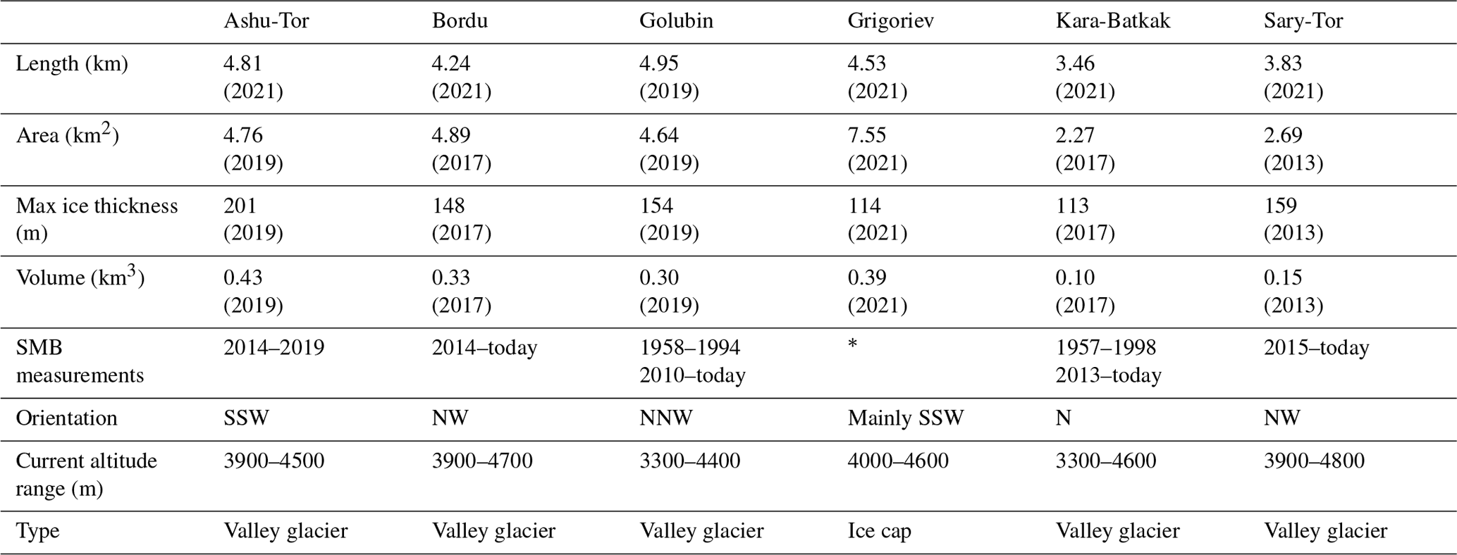
* Surface mass balance episodically measured (Mikhalenko, 1989; Dyurgerov, 2002; Arkhipov et al., 2004; Fujita et al., 2011).
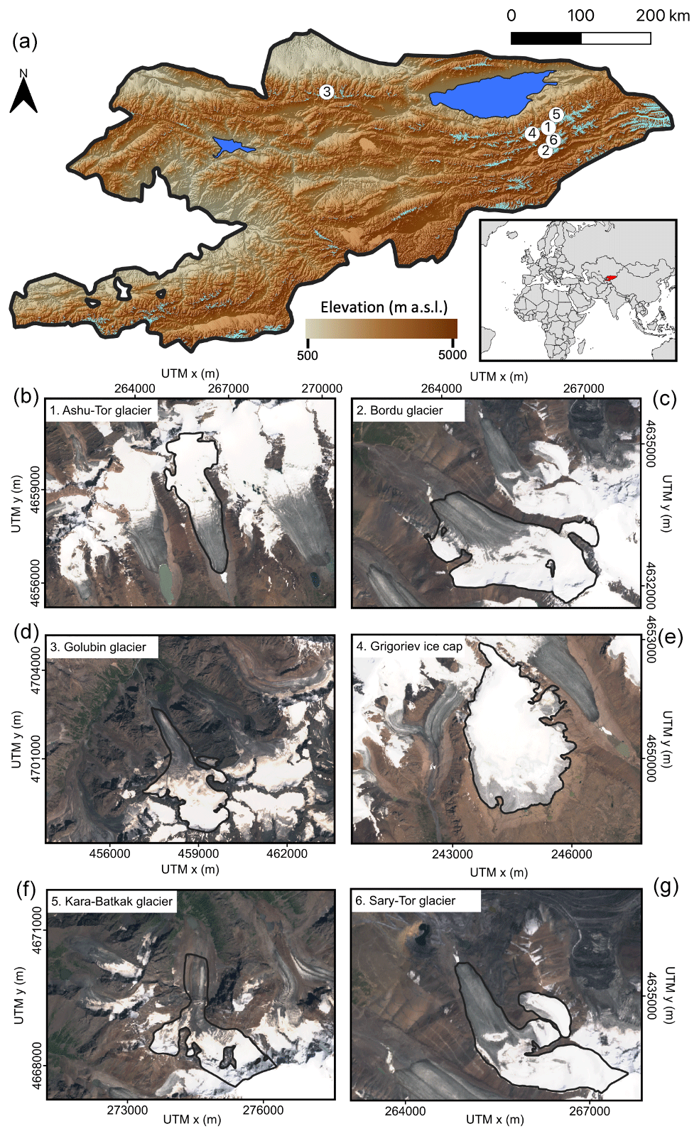
Figure 1(a) Selected glaciers and their location in Kyrgyzstan. The DEM is the Shuttle Radar Topography Mission (SRTM). All glaciers of the Randolph Glacier Inventory version 6 (RGI v6) are shown in pale blue (RGI consortium, 2017). (b)–(g) Six selected glaciers. The background satellite images are from Sentinel-2 data acquired in July/August 2021. The black outlines of the glaciers show the extent in 2021, determined by manual delineation.
2.2 Climatic setting and drainage
The continental climate of the Tien Shan is characterized by a strong seasonal variation in precipitation, a large west-to-east gradient in total precipitation, and large seasonal amplitudes of air temperatures (Barandun and Pohl, 2023). Precipitation is highest in spring and summer, accounting for about 75 % of the annual total (Kutuzov and Shahgedanova, 2009). This precipitation is primarily caused by convection and a strengthening of instability caused by cold, moist air mass influxes from the west (Aizen, 1995). In winter, the advection of precipitation by westerly flow is mostly blocked by the strong influence of the Siberian high. The Ashu-Tor, Bordu, and Sary-Tor glaciers, as well as the Grigoriev ice cap, are all located in the Arabel Plateau system with a very limited amount of annual precipitation (∼ 320 mm yr−1 at 3600 m a.s.l.) (Van Tricht et al., 2021b). These ice masses feed several of Central Asia's largest rivers, such as the Naryn River, which flows in the Syr Darya, draining westwards towards the Aral Sea basin (Blomdin et al., 2016). Winter precipitation in the central area of the Tien Shan accounts for only 8 %–10 % of the annual total (Aizen, 1995). This means that the ice masses are characterized by a simultaneous occurrence of main accumulation and main ablation in spring and (early) summer, making them very sensitive to temperature changes in spring and summer (Fujita, 2008; Van Tricht et al., 2021b). A rise in temperatures during this period not only causes increased melting but also causes a reduction of snow and a decrease in albedo.
The Golubin glacier is located further to the north-west of Kyrgyzstan, in an area which is characterized by a larger amount of annual precipitation of up to 550 mm yr−1 at 2000 m a.s.l (Aizen et al., 2006). The greater amount of annual precipitation can be explained by the larger influx of moisture from the north-west, in which direction the Kyrgyz Ala-Too is oriented. In addition to a larger amount of precipitation, precipitation is also more focused in spring (March and April), which implies that summer precipitation events are less important on this glacier. Meltwater from glaciers in the area feeds the endorheic basin of the Chu River, which is the major irrigation and water supply for northern Kyrgyzstan, including the capital Bishkek and the Kazakh steppe.
The Kara-Batkak glacier, finally, is located at the northern slopes of the Terskey Ala-Too, which are more exposed to moisture originating from Lake Issyk-Kul. The glacier area is therefore characterized by a wetter climate (on average 600–700 mm yr−1 at 2600 m a.s.l.) (Van Tricht et al., 2021b). Meltwater from glaciers in this area drains towards the endorheic basin of Lake Issyk-Kul.
2.3 Meteorological data
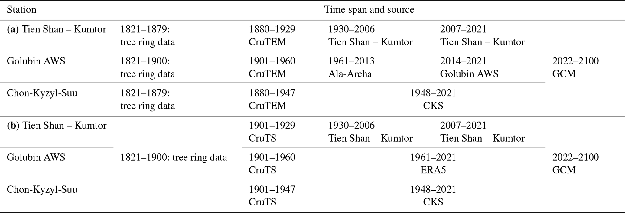
Three meteorological time series are used to represent the climate near the six different ice masses (Tien Shan – Kumtor, Chon-Kyzyl-Suu, and Golubin automatic weather station (AWS)) (Table 2). The reconstructed data series of Tien Shan – Kumtor is used for the Ashu-Tor glacier, the Bordu glacier, the Grigoriev ice cap, and the Sary-Tor glacier. For the Kara-Batkak glacier, the dataset of Chon-Kyzyl-Suu (CKS) is used. All different time series used to create the meteorological dataset are debiased using overlapping periods. For a detailed description on how the data time series for these two stations have been created, we refer to Van Tricht et al. (2021b).
Concerning the Golubin glacier, a meteorological dataset is created for the location of the AWS at 3300 m a.s.l. near the Golubin glacier (Hoelzle et al., 2017) (Table 2). Directly measured temperatures at this AWS are used for 2014–2021. For 1961–2013, anomalies derived from measured temperatures at the Ala-Archa station (situated at 2145 m a.s.l. ∼ 10 km from the front of the Golubin glacier) are used. For the 1901–1960 period, data from the CruTEM (Climatic Research Unit gridded land-based TEMperature database) are taken, and between 1750 and 1900, data from tree rings are used (see Van Tricht et al., 2021b, for more information) (Table 2). For precipitation, we rely on ERA5 data, which are scaled to match the measured mean annual precipitation of the Ala-Archa station for the overlapping period, for 1961–2021. The CruTS (Climatic Research Unit gridded Time Series) dataset is considered for the 1901–1960 period. To represent the precipitation during 1750–1900, data from tree rings are used (Solomina et al., 2014) (Table 2). Like for the other two datasets, the different time series used for the Golubin AWS dataset are debiased using overlapping periods and matched for interannual variability using the standard deviation in the common period.
Table 2Temperature (a) and precipitation (b) datasets and their time spans used in this study.
2.4 Little Ice Age
Glaciers and ice caps in the Kyrgyz Tien Shan repeatedly advanced and retreated throughout the Holocene. The latest period of significant advance was caused by the LIA, and it was dated to 1730–1910. In most areas, several moraines belong to the LIA, indicating different stages of glacial stagnation and advances within this period. However, a majority of terminal and side moraines were formed in the middle of the 19th century (Solomina et al., 2004; Li et al., 2017). In this study, we consider the 1820–1850 average climatic conditions to represent the end of the LIA period.
2.5 Future climate
For the future climate (2022–2100) (Table 2), we rely on climate change projections from multiple global climate models (GCMs) which participated in the sixth phase of the Coupled Model Intercomparison Project (CMIP6) (Table 3), available through the Earth System Grid Federation (ESGF) archive. Only the models with a transient climate response inside the 66 % likelihood range are considered (Hausfather et al., 2022) (up to 18 GCMs). Five shared socioeconomic pathways (SSPs) are considered, which represent a peak and decline scenario (SSP1-1.9 and SSP1-2.6), two medium scenarios (SSP2-4.5 and SSP3-7.0), and a high emission scenario (SSP5-8.5). These new climate scenarios have been developed for the Sixth Assessment Report of the Intergovernmental Panel on Climate Change (IPCC AR6).
For every available GCM and every meteorological station, the data are downloaded for both historical runs (1984–2014) and future projections (2022–2100). The grid cell closest to the meteorological stations is considered. Each GCM has a specific spatial resolution of between 0.93∘ and 2.50∘ (Table 3). The data from every individual GCM are then converted into anomalies for temperature and into ratios for precipitation, with respect to the overlapping historical period (1984–2014), and scaled to match the standard deviation of the observations of the specific meteorological datasets (see Sect. 2.3). Then, for every SSP scenario, the monthly temperature anomalies and precipitation ratios are averaged over all models, resulting in a multi-model mean time series combining up to 18 different GCMs (see Table 3). Next, to account for interannual variability, the data are rescaled using a sequence of historical observations. Finally, as was done for the historical period (Van Tricht et al., 2021b), the monthly data series are downscaled to hourly resolution by using an observed data sequence between 2007 and 2021 for the Tien Shan – Kumtor and Chon-Kyzyl-Suu dataset and between 2014 and 2021 for the Golubin AWS dataset.
Table 3CMIP6 global climate models (GCMs) used for the climate projections. The X indicates that the GCM contains data for this SSP scenario.
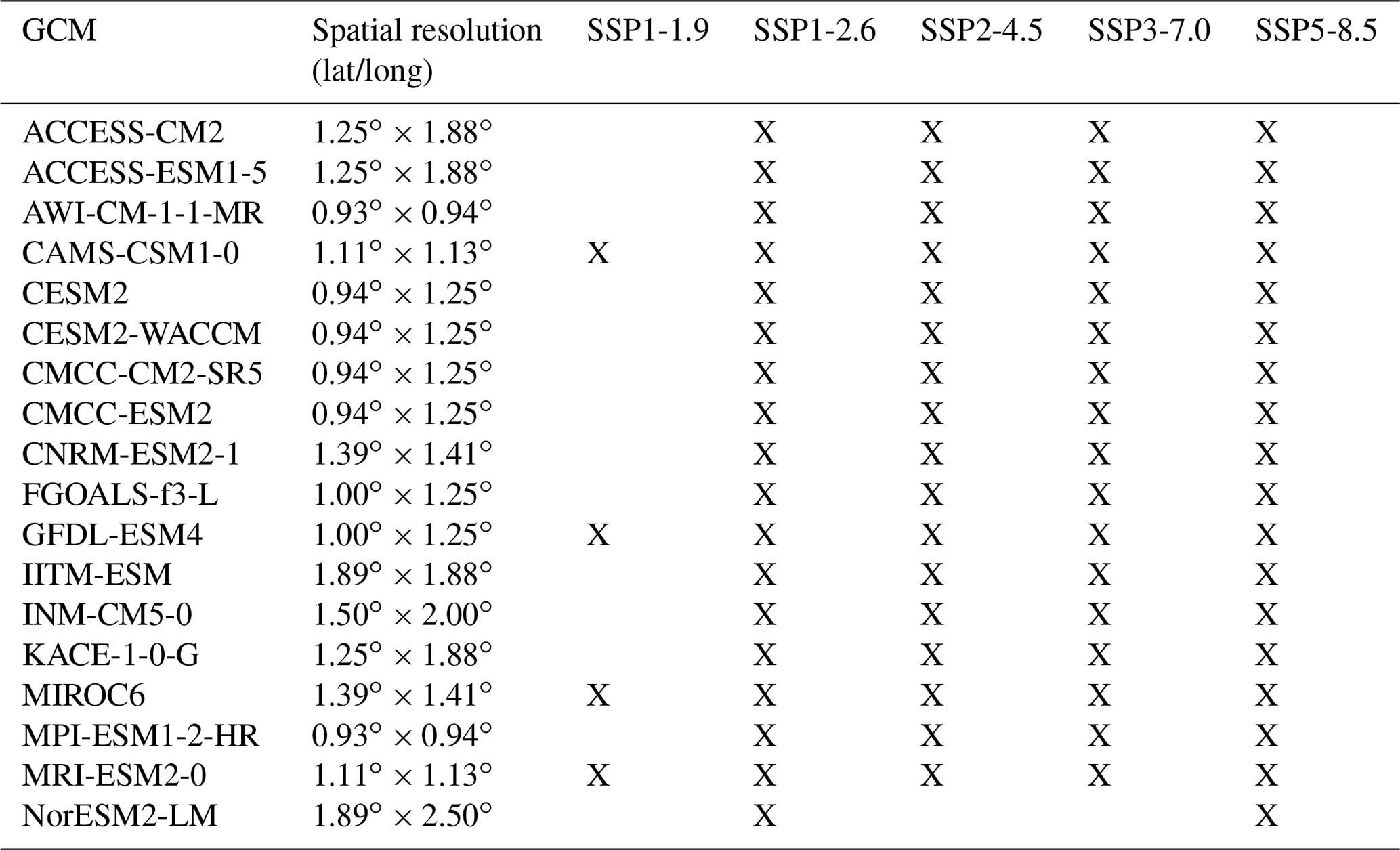
In addition, a “no change” scenario is created for which we use a random shuffling of the years between 2001 and 2021 until 2100. The effect of a lower resolution of the GCMs compared to regional climate models (RCMs) is expected to be limited, as we consider anomalies and because we impose climatic variability based on observations. Next to that, by combining multiple GCMs, the influence of errors and uncertainties of individual models are assumed to be reduced strongly, which is beneficial for the reliability of future projections. Only for the SSP1-1.9 scenario was a limited number of GCMs (4) available at the time of the experiments. For all three meteorological datasets, temperatures are projected to increase substantially compared to the 2001–2021 mean, with values between +0.7 ∘C for the SSP1-1.9 scenario and up to +5.7 ∘C for the SSP5-8.5 scenario (Fig. 2). The projected evolution of the total precipitation shows a slight but insignificant increase for the Tien Shan – Kumtor location and no real trend for the two other locations (Fig. 2). In addition to conducting simulations using the multi-model mean of every SSP scenario, we further generate two additional scenarios for each SSP. These scenarios are designed to incorporate a gradual increase or decrease in temperature, aiming to reach approximately the standard deviation of the projected temperatures at the end of the century across the various GCMs. This approach is implemented to account for the inherent uncertainty between the different GCMs and provides a more comprehensive representation of the possible temperature variations within each SSP. For precipitation, we always consider the multi-model mean.
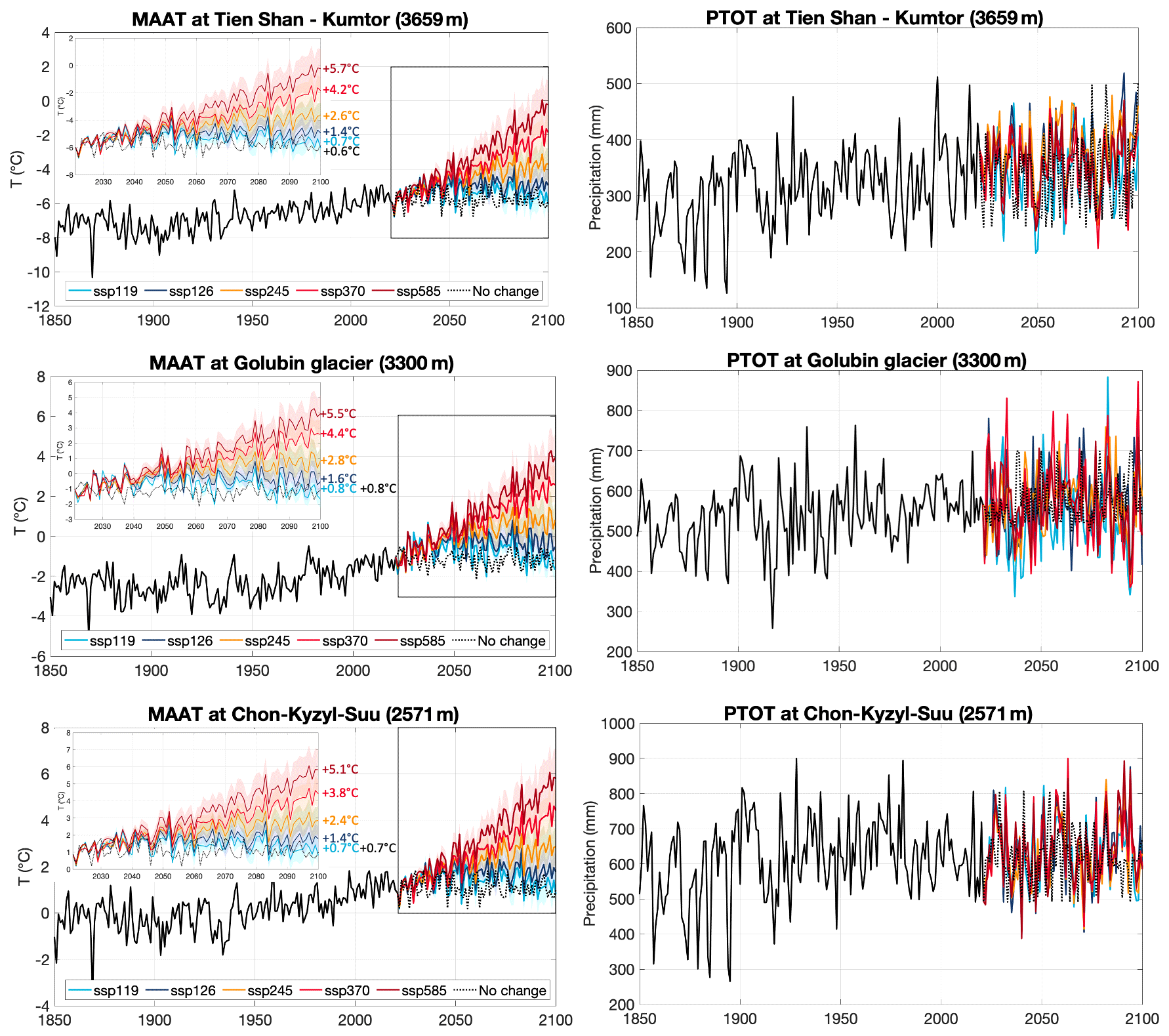
Figure 2Evolution of the mean annual air temperature (MAAT) and the yearly total precipitation (PTOT) between 1850 and 2021 as well as projections until 2100 under different climate scenarios for the three locations. The insets are enlargements of the future temperature. The numbers at the right side of the insets indicate the average warming in 2090–2100 for every scenario with respect to the 1960–1990 average.
3.1 Higher-order ice dynamic flow model
A three-dimensional higher-order thermo-mechanical ice-flow model (3D HO model) is used to model the ice flow in this study. In the model, both longitudinal and transverse stress gradients are considered (Zekollari et al., 2013), in contrast to Shallow Ice Approximation (SIA) models (Hutter, 1983). The 3D HO model assumes cryostatic equilibrium in the vertical, implying that vertical resistive stresses are neglected (Pattyn, 2003), in contrast to full-Stokes models that incorporate all stresses (Jouvet et al., 2011). Further, it is also assumed that the horizontal gradients of the vertical velocity are much smaller than the vertical gradients in the horizontal velocity. This reduces the processing compared to a full-Stokes model, as only the horizontal velocity components are solved for. In the following, the applied model is briefly described. A more detailed description of the model can be obtained from Fürst et al. (2011). The vertical velocity component is derived from the incompressibility condition. Nye's generalization of Glen's flow law (Eq. 1) with a power exponent n of 3 is used to quantify the ice deformation and the corresponding flow velocity due to internal deformation based on the stresses that act on it:
η is the effective viscosity of the ice (Eq. 2), which is defined via the second invariant of the strain rate tensor (Eq. 4). is a small offset (10−30) that ensures finite viscosity. The symbols “i” and “j” represent the space derivative with respect to the ith and jth spatial components. The flow rate factor A(Tpmp) is a function of ice temperature with respect to the pressure melting point (Eq. 3). E is an enhancement factor which is used for calibration (see Sect. 3.4). The tuning of the enhancement factor is an implicit way to include the softening effect due to factors such as water content and impurity content (Huybrechts, 1990). For temperatures lower than −10 ∘C, Pa−n yr−1 and Q=60 kJ mol−1, while for temperatures larger than −10 ∘C, Pa−n yr−1 and Q=139 kJ mol−1. R is the gas constant (8.31 J mol−1 K−1). Tpmp is the ice temperature relative to the pressure melting point (homologous temperature). is the effective strain rate as the second invariant of the strain rate tensor. The strain rate tensor is defined in terms of velocity gradients (Eq. 5) with u representing the three-dimensional components of the velocity vector. Further, in the ice-flow model, a Weertman-type sliding law is implemented (Eq. 6). Here, the basal sliding velocity (ub) is proportional to the basal drag (τb) to the third power:
The basal drag corresponds to the sum of all basal resistive stresses. Asl is the sliding parameter, which is defined as a constant in the model and calibrated for every specific ice mass (see Sect. 3.4). There is no basal sliding when the basal ice temperature is below the pressure melting point. A full 3D calculation of the ice temperatures is performed at all time steps and for every location. This calculation involves vertical diffusion, three-dimensional advection, and heating caused by deformation and basal sliding, following the methodology described in Van Tricht and Huybrechts (2022). The ice temperatures of the surface layer are determined based on the average annual air temperature and parameterizations that consider the effects of warming due to refreezing meltwater and snow insulation, as well as the effect of the removal of ice at the surface in the ablation area. The study of Van Tricht and Huybrechts (2022) provides the necessary parameters to prescribe these processes: 41 ∘C (m w.e.)−1 for refreezing meltwater and 22 ∘C (m w.e.)−1 for insulating snow, which are considered to be constant in space and time for the six ice masses. At the bottom of the ice, heat is produced by geothermal heating and friction caused by basal sliding and ice deformation. A geothermal heat flux of 50 mW m−2 is prescribed. The model is run on a 25 m resolution with 21 equally spaced layers in the vertical. Calibration consists of tuning the enhancement factor and the basal sliding parameter to minimize differences between modelled and observed ice thickness. The ice-flow model is coupled to a simplified surface energy balance model that calculates the spatio-temporal distribution of the surface mass balance (see Sect. 3.2). The continuity equation (Eq. 7) is used to link both models:
with H representing the ice thickness, the vertically average horizontal velocity vector, ∇ the 2D divergence operator, and ms the surface mass balance. The higher-order velocity field and the changes in ice thickness are calculated twice a week, while the surface mass balance is updated annually.
3.2 Surface mass balance model
The selected surface mass balance model is the simplified energy balance model that has been optimized, calibrated, and used in Van Tricht et al. (2021b) for different glaciers in the Tien Shan. The model is based on the net energy balance at the surface with incoming solar radiation, albedo, and transmissivity, as well as two tuning parameters (C0 and C1) representing the sum of the net longwave radiation balance and the turbulent sensible heat exchange. A representation of the surface elevation is used to calculate the insolation based on local slope and aspect, shadow, and the elevation-dependent temperature and precipitation.
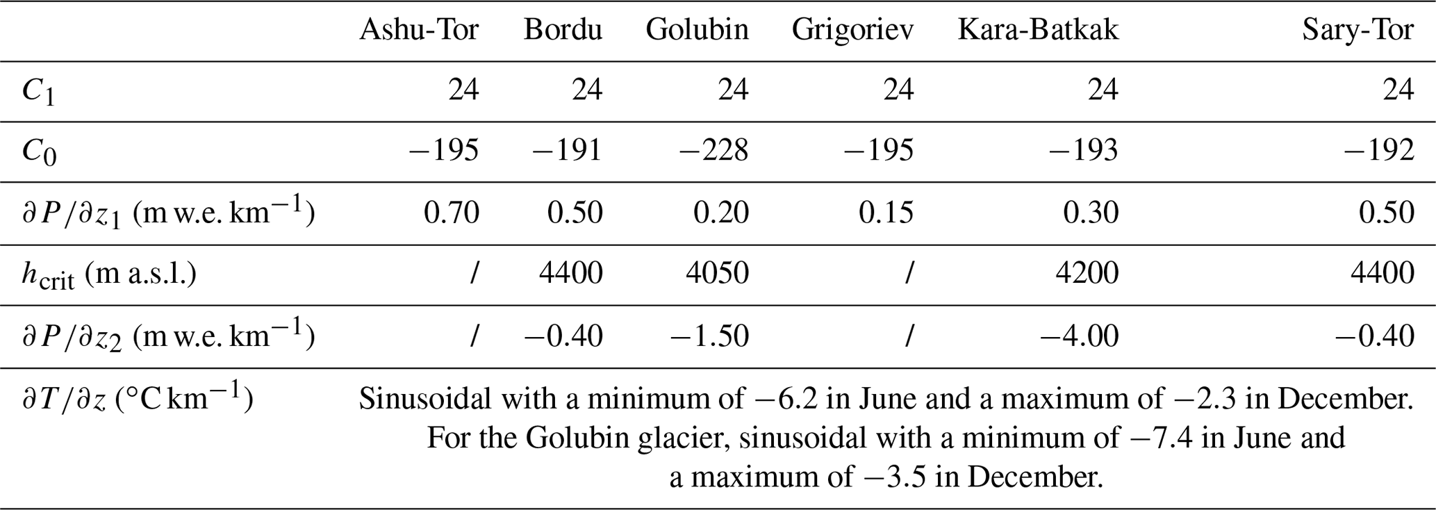
Calibration of the model is carried out based on measured mass balances at stakes which are interpolated to average values for elevation bands of 100 m. The input data of the surface mass balance model are limited to hourly precipitation and temperature data of meteorological stations in the vicinity of the ice masses and a surface DEM. An overview of the most important parameters of the surface mass balance model is given in Table 4. C1 is kept fixed at 24 as was found in Van Tricht et al. (2021b). C0 is initially taken from Van Tricht et al. (2021b) and Van Tricht and Huybrechts (2022) and then further adjusted based on mass balance observations of the 2020/21 season. All other parameters are reproduced from Van Tricht et al. (2021b). A sinusoidal course of the lapse rate (vertical temperature gradient) is created, based on the monthly lapse rates provided by Aizen et al. (1995), to ensure a smooth transition during the year (see Table 4). For some glaciers, two precipitation gradients are used (Table 4) to account for moisture depletion and wind erosion in the upper reaches above a certain elevation (hcrit). To correctly reproduce the surface layer temperatures needed to model the englacial temperatures, the amount of refrozen water and the maximum snow thickness in May are estimated, following the approach described in Van Tricht and Huybrechts (2022).
Table 4Overview of the calibrated parameters. For some ice masses, two different precipitation gradients are adopted, indicated by the subscript 1 and 2, to account for moisture depletion and wind erosion in the upper reaches. hcrit is the elevation above which the second precipitation gradient is used.
3.3 Geometric data
The input data of the ice-flow model are limited to a bedrock DEM which is determined by subtracting the measured and reconstructed ice thickness of the different ice masses (Petrakov et al., 2014; Van Tricht et al., 2021a; Van Tricht et al., 2023) from a surface DEM as close as possible to the date of the ice thickness data. To represent the surface elevation, the TerraSAR-X add-on for the Digital Elevation Measurement mission (TanDEM-X) (2013) is selected. In the frontal areas for all glaciers, and for the entire Bordu glacier, Grigoriev ice cap, and Sary-Tor glacier, the surface DEM is derived from photogrammetrically created digital surface models (DSMs) from UAV images in 2021, created following the approach described in Van Tricht et al. (2021c). A LIA mask is created to avoid ice flowing over ridges away from the glaciers in the accumulation areas. This mask is determined by manual delineation of the LIA ice boundary based on unique and well-recognizable moraines on satellite images from Sentinel and Landsat. The LIA extent and the retreat of the Golubin glacier are adopted from data presented in Aizen et al. (2006), which date back to tacheometric surveys from the mid-19th century (Venukov, 1861). In 1861, the Golubin glacier terminus was located in a deep canyon at 2900 m a.s.l. (Venukov, 1861; Aizen et al., 2006). Between 1861–1913, the terminus retreated to 3050 m a.s.l. From 1913 to 1949, the terminus retreated to an elevation of 3150 m, and by 1963 it reached 3250 m a.s.l. Between 1958 and 1982, small annual oscillations of the terminus position were measured (Aizen et al., 1983). From 1982 onwards, the terminus retreated in a rather constant way.
3.4 Calibration of the flow parameters
Our initial iterative minimization procedure aims to simulate the ice thickness distribution as close as possible to the observations. The latter concerns the ice thickness distribution of the different ice masses created from measurements and reconstruction for the Ashu-Tor (2019), Bordu (2017), Kara-Batkak (2017), and Golubin glaciers (2019) (Van Tricht et al., 2021a); the Grigoriev ice cap (2021) (Van Tricht et al., 2023); and the Sary-Tor glacier (2013) (Petrakov et al., 2014) (see Table 1). To do this, the coupled velocity and temperature model is run forward until a steady state is reached using the average 1960–1990 climatic conditions. The latter period is considered to be the climate regime resulting in the present-day ice geometry, considering a typical response time of 30–60 years (Jóhannesson et al., 1989). To take into account a mismatch of the steady-state assumption, the surface mass balance is modified by implementing a temperature and/or precipitation bias to achieve the best possible fit between the modelled extent of the ice masses and the observed ice mass extent (length calibration).
When a steady state with the desired length is reached (zero ice thickness change), the obtained ice thickness distribution is compared with the measured ice thickness distribution, and the RMSE is calculated. Subsequently, the basal sliding parameter (Asl) and the enhancement factor (E) are adjusted within a predefined range, and the model is run until a new steady state is reached for the new parameter combination. Calibration then consists of looking for the combination of parameters with a minimal RMSE between modelled and observed ice thickness. The enhancement factor is varied between 1 and 15 in steps of 1, and the basal sliding parameter is varied between and Pa−3 m2 yr−1 for a predefined set of values. The parameter combination with the minimum RMSE for every ice mass is used for the initial runs. In the dynamical calibration procedure (see Sect. 4.2), the flow parameters might be further adjusted by comparing time-dependent modelled ice thickness and velocities (if available) with observations.
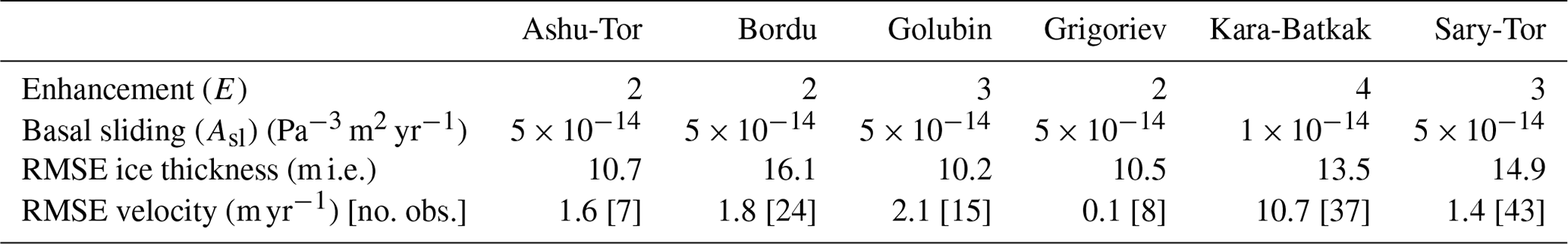
The optimal enhancement factors and basal sliding parameters are close to each other (Table 5), which increases the confidence in the calibrated values. The RMSE between modelled and measured ice thickness is for all ice masses between 10.2 and 16.1 m, while the mean error (ME) is between −2.3 and 6.2 m. With average ice thicknesses of about 100 m, this shows that the modelled ice thicknesses are within 10 % of the observations. The RMSEs of the modelled velocities are of the order of 1–2 m yr−1, except for the Kara-Batkak glacier for which the RMSE is larger (11 m yr−1). With regard to the latter, the velocities are higher (up to 60 m yr−1), and for the highest values there are some mismatches that strongly affect the RMSE (see Fig. 6). For the comparison between modelled velocities and observed velocities of the Grigoriev ice cap, we use the stake locations of Fujita et al. (2011) from 2006–2007 and one additional velocity observation that could be created based on feature tracking on the eastern outlet glacier using Sentinel satellite images of 2017 and 2018. It must be noted that the stakes were only located in the upper (and slower) part of the ice cap.
To obtain a reliable prognosis of the future evolution of the selected ice masses, it is crucial to simulate their historical retreat because the current ice masses are still responding to past changes. Therefore, the ice-flow model is first dynamically calibrated to reproduce the observed retreat since the end of the LIA. For this purpose, outlines of different years, which are derived from satellite images (Landsat, Sentinel) and from previous reconstructions, are used.
4.1 Ice geometry at the end of the LIA
The starting point of the historical reconstructions is the end of the LIA, which is set at 1850 based on obtained lichenometric dates of LIA moraines (Savoskul and Solomina, 1996; Solomina et al., 2004; Li et al., 2017). To start, the coupled model is run for constant average 1820–1850 climatic conditions until a steady state is reached. Then, the obtained ice masses are compared with the LIA extent derived from clearly visible unique end moraines on satellite images. Based on this comparison, a temperature and/or precipitation bias is searched for and applied to acquire the LIA geometry of all ice masses (Table 6). These biases are determined by assessing combinations between ±0–0.2 ∘C for temperature and ±0 %–15 % for precipitation, while keeping the impact of the biases on the modelled ice thickness low. The small biases needed to reconstruct the LIA indicate a rather good reliability of the meteorological data used to represent the end of the LIA.
Table 6Reconstructed ice volume and maximum ice thickness at the end of the Little Ice Age (1850) of the different ice masses. A temperature and/or precipitation bias is used to acquire the supposed LIA extent.
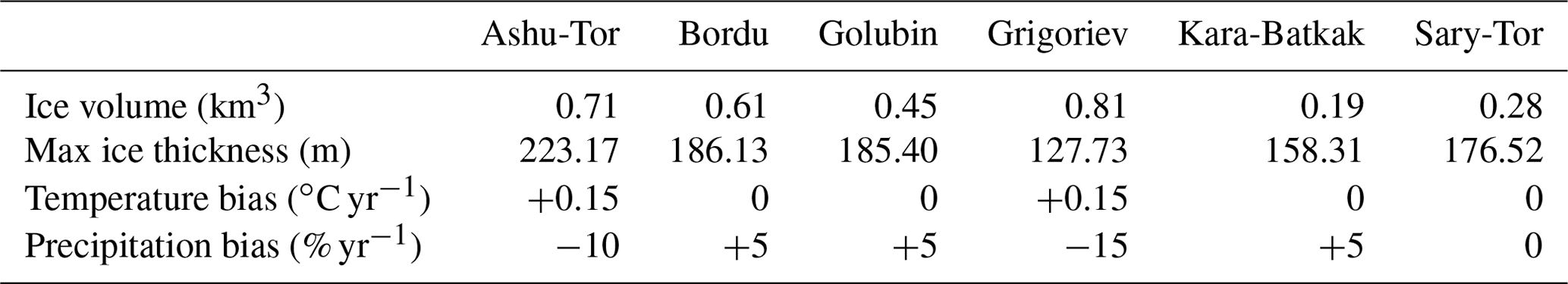
The 1850 geometry of the different ice masses resulting from the calibrated ice-flow model is significantly larger than the present-day outline, especially in the frontal areas (Fig. 3). Higher up the ice masses, at the altitude of the current accumulation areas, the ice geometry has changed little, both in thickness and in extent. The Bordu and Sary-Tor glaciers, which are located in neighbouring valleys, have a gently sloping bedrock, so they had very similar thicknesses and sizes at the end of the LIA. The Ashu-Tor glacier is situated on a flat bedrock, which causes this glacier to be characterized by a distinctly thicker ice body. The Kara-Batkak glacier occupies a much greater elevation interval and has a steeper bedrock. Therefore, this glacier has always been thinner compared to the other ice masses. However, at the end of the LIA, the maximum ice thickness was 30 % more than the current maximum. The Golubin glacier extended at the end of the LIA much more to the north-west, ending at a steep north-facing valley side (Venukov, 1861). The Grigoriev ice cap was especially larger at the southern margin and also merged with the Chontor glacier to the west and the Popova glacier to the east (both are not modelled separately in this study).
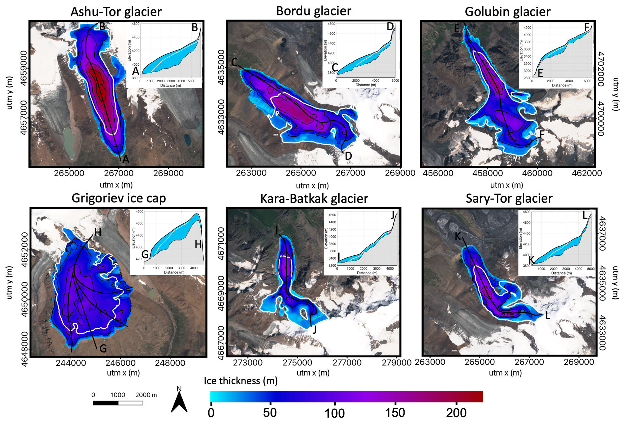
Figure 3LIA geometries of the different ice masses, reconstructed with the ice-flow model and 1820–1850 climatic conditions. The inset shows the bedrock and surface profile along the main flowline, indicated with a black line for the LIA geometry and with a white line for the measured and reconstructed ice thicknesses. The white outline represents the extent of the ice mass at the time of the measurements. The background satellite images are from Sentinel-2 data acquired in July/August 2021.
4.2 Ice evolution between 1850 and 2021
Then, starting from the obtained steady-state LIA geometry (Fig. 3), the surface mass balance is annually calculated for the evolving modelled surface topography using the energy balance model to simulate the historical evolution of the ice masses between 1850 and 2021. The modelled length of the main flowline is compared with lengths derived from satellite data. Since the Grigoriev ice cap does not have a unique main flowline, as is typical for an ice cap, we chose to use four separate flowlines and dynamically calibrate for the mean length of the flowlines. By comparing with the intermediate extents, a temperature and/or precipitation bias is searched for and used to match the historical modelled extents optimally with the observed extents.
This bias implicitly accounts for uncertainties in the mass balance model and errors in the climatic records. The bias varies in time and appears to be necessary to closely reproduce the observed retreat of the different ice masses in the past, where reconstructed climatic data are characterized by greater uncertainty. For at least the last 3 decades, which corresponds to a typical response time of the studied ice masses (Jóhannesson et al., 1989), no biases need to be applied to correctly reconstruct the observed retreat. This suggests that the surface mass balance derived for the recent (more accurate data from local measurements) decades provides a more correct forcing for the ice-flow model, which increases the confidence in the calibrated model used in this study.
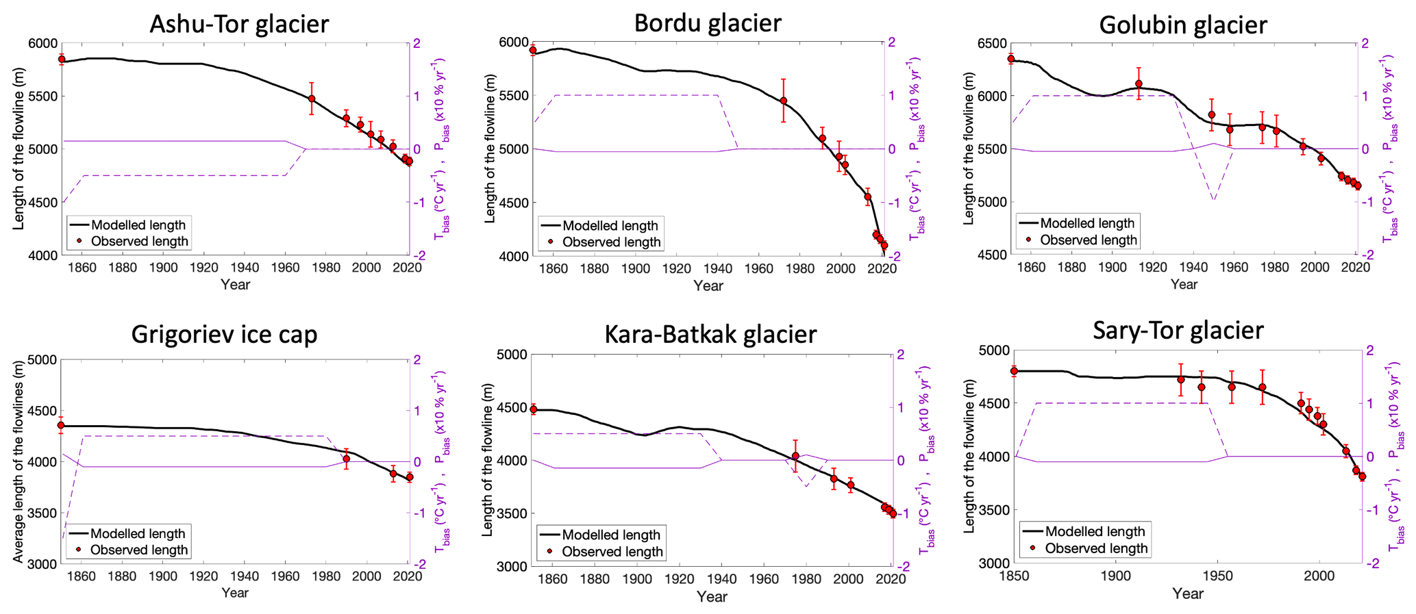
Figure 4Reconstructed retreat of the different ice masses along the main flowline and observed extent (red circles). The temperature bias (∘C yr−1) is shown as the solid purple line, while the precipitation bias is shown as the dashed purple line (×10 % yr−1). The red dots represent the observed length. The confidence interval (red whiskers) is determined based on the quality and the resolution of the satellite data used for the determination of the front positions.
In the second half of the 19th century, the ice masses only slightly retreated (Fig. 4). Then, in the beginning of the 20th century, lower temperatures ensured for some of the ice masses a period of (slight) advance, which is most noticeable for the Golubin glacier and the Kara-Batkak glacier, which are characterized by the lowest response time following the approach of Jóhannesson et al. (1989). In the second half of the 20th century and especially after 1970, the retreat clearly accelerated for all of the ice masses.
4.3 Comparison with observed ice thicknesses and surface velocities
We first evaluate the modelled ice thickness with the ice thickness measurements and reconstructions reported in previous studies (Petrakov et al., 2014; Van Tricht et al., 2021a, 2023). The results reveal a strong agreement between the modelled thickness and the measured and reconstructed thickness, with in general small differences, especially for the areas where ground-penetrating radar (GPR) measurements were conducted (Petrakov et al., 2014; Van Tricht et al., 2021a, 2023). Overall, the RMSE and mean error (ME) are found to be low (Fig. 5). This is a logical outcome, considering that the ice thickness observations were utilized to calibrate the flow parameters.
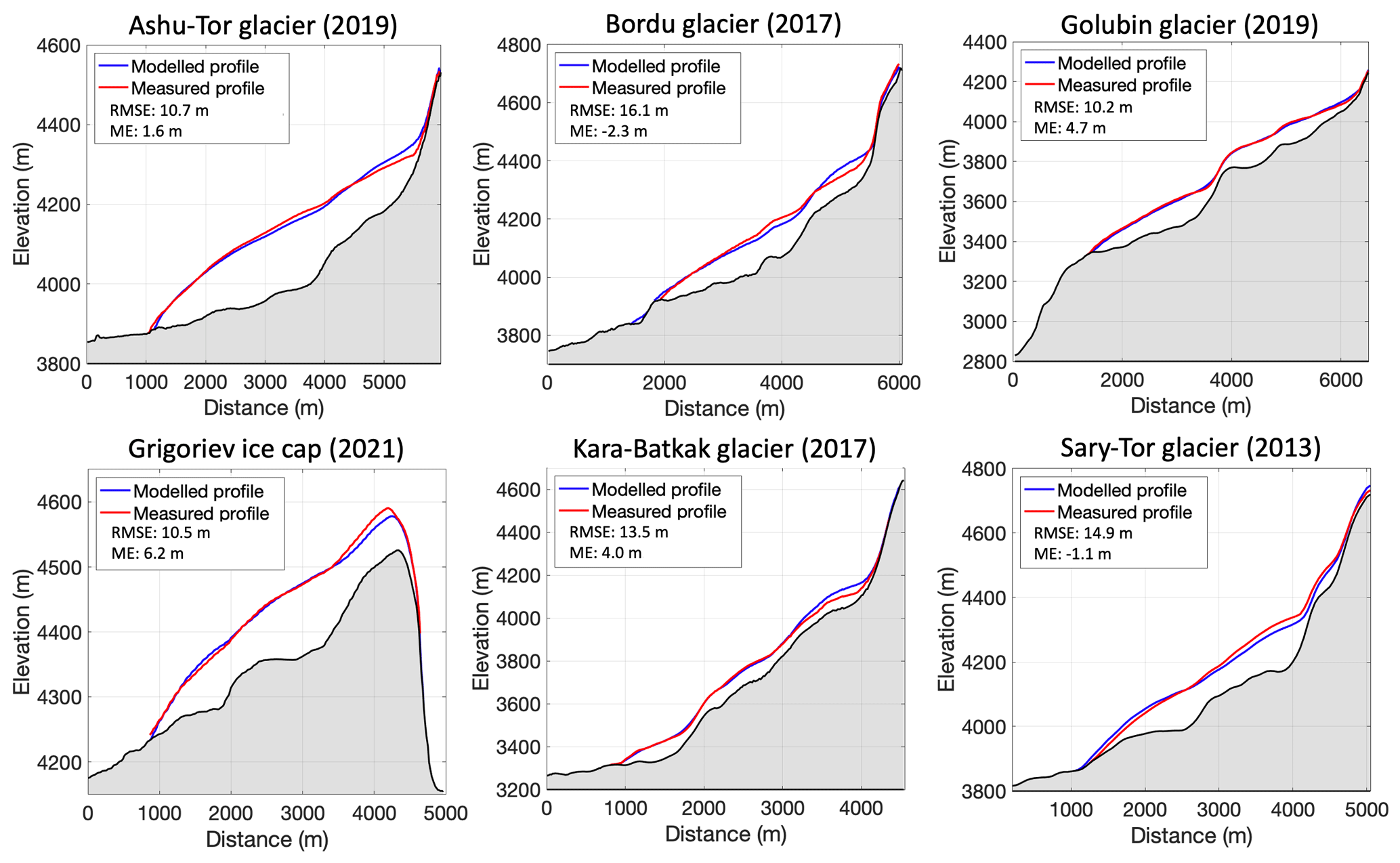
Figure 5Comparison between the modelled ice thickness profiles with measured and reconstructed ice thicknesses.
Subsequently, we assess the modelled surface velocities by comparing them with the point surface velocities derived from stake displacements and the displacements of identifiable features such as supraglacial boulders captured on UAV and satellite images for various years spanning from 2012 to 2021. Like for the ice thickness, we find a close agreement with low values of the RMSE and the ME (Fig. 6). In addition, there does not seem to be a bias towards higher or lower velocities for any of the ice masses compared to the observations.
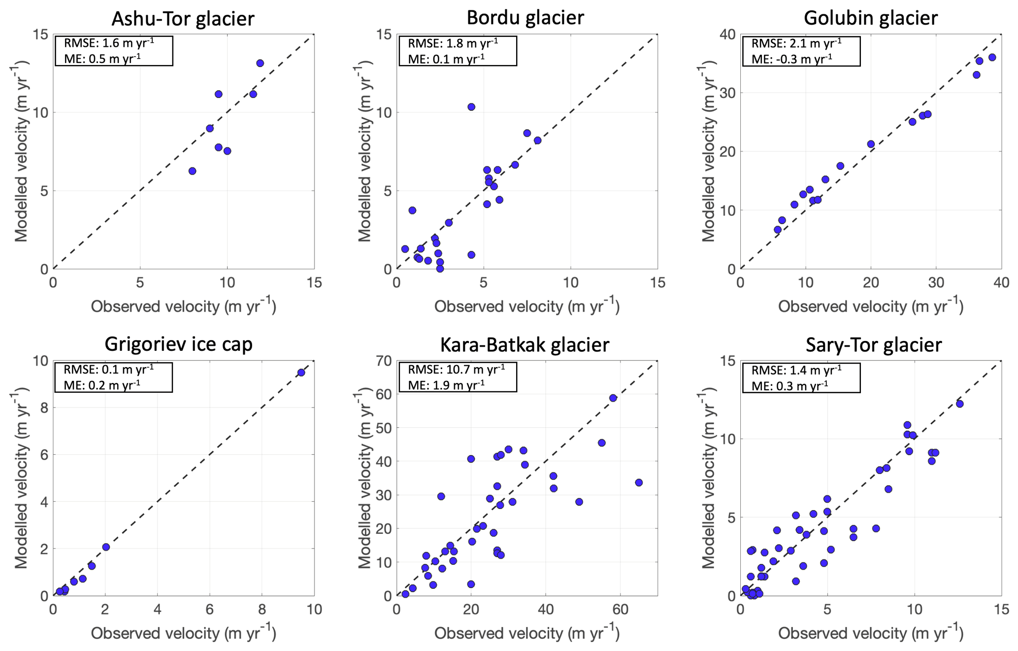
Figure 6Comparison between the modelled surface velocities and measured velocities. The diagonal is the 1:1 line.
4.4 Validation with geodetic mass balances and ice thickness in 2000
As an individual and independent validation of our study, the historical reconstructions of the ice masses are compared with geodetic mass balances for multiple periods (Table 7). In general, we find a close correspondence that is mostly within the uncertainty ranges of the geodetic mass balances. Only for the Kara-Batkak glacier are there larger discrepancies which might be caused by the absence of the highest part of the accumulation area in the RGI version 6.0 dataset that is used to derive most of the geodetic mass balances. For the latest dataset, which comprises the elevation change rate of 2000–2019 (Hugonnet et al., 2021), we find for all ice masses a very close correspondence, except for the Ashu-Tor glacier (Table 7). The geodetic value for this glacier is very negative and much lower than for the surrounding glaciers. The Ashu-Tor glacier might be affected by local climate characteristics that are not captured by the Tien Shan – Kumtor weather station or our mass balance model. The Kara-Batkak glacier is clearly characterized by the least negative modelled elevation change rate as geodetic mass balance (Table 7), which matches with the slower and more limited retreat and melting of this glacier (see also Fig. 7). As an additional validation, we also compare the modelled ice thickness in 2000 with ice thicknesses derived using the Shuttle Radar Topography Mission (SRTM) DEM. In general, we find low RMSE values: 14.9 m ice equivalent (i.e.) for the Ashu-Tor glacier, 16.4 m i.e for Bordu glacier, 12.3 m i.e. for Golubin glacier, 15.2 m i.e for the Grigoriev ice cap, 13.2 m i.e. for the Kara-Batkak glacier, and 16.2 m i.e. for the Sary-Tor glacier.
Table 7Validation between geodetic mass balances and modelled elevation change rates for different periods. Both values are given in m w.e. yr−1. The cells displaying modelled values beyond the range of geodetic mass balance ± uncertainty are highlighted in bold.
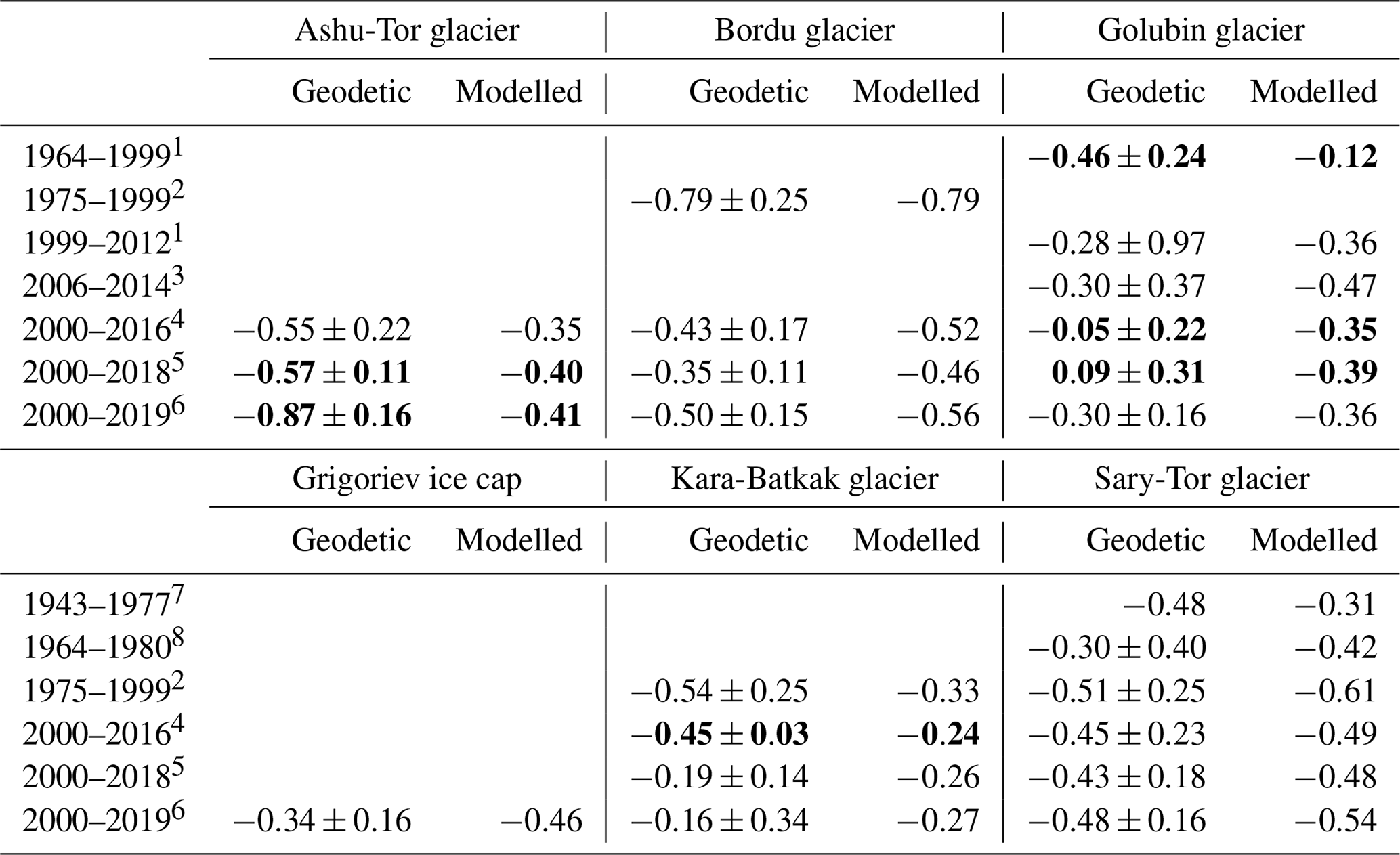
1 Bolch et al. (2015). 2 Pieczonka and Bolch (2015). 3 Barandun et al. (2018). 4 Brun et al. (2017). 5 Shean et al. (2020). 6 Hugonnet et al. (2021). 7 Aizen et al. (2007). 8 Goerlich et al. (2017).
5.1 Projected ice volume and area for 2022–2100
Under all considered SSP scenarios, the results show a strong volume and area loss for all ice masses (Fig. 7). In the case of the SSP5-8.5 scenario, the ice masses entirely disappear by 2100, except for the Kara-Batkak glacier for which 3 % of the 2021 volume remains, located in the upper area (Fig. 9). The rate of decline of the ice masses varies, although the majority of the ice masses already disappear by 2080.
For the other SSP scenarios, there are some notable differences in the responses of the ice masses to the imposed climate. The Grigoriev ice cap retreats to (almost) 0 % of its current volume, except for SSP1-1.9 (Fig. 7). Even under the 2001–2021 climate, only 33 % of the present-day ice volume remains by 2100. This very strong retreat of the Grigoriev ice cap can be explained by the limited altitudinal extent or the “small ice cap instability”. The Grigoriev ice cap is located on top of a rather flat mountain, which means that the ice cap cannot retreat to higher elevations (Van Tricht et al., 2023). At present, the equilibrium line altitude (ELA) is located around 4350–4400 m, which is only 100–150 m below the summit. A more negative mass balance in the future causes a thinning and a lowering of the surface, which amplifies the melting (positive feedback effect). The Grigoriev ice cap is therefore largely dependent on its own height to sustain itself, while glaciers can migrate upwards or downwards when reacting to a changing climate. Under SSP2-4.5, the ELA already rises to the summit before the middle of the 21st century (Fig. 8).
The evolution of the Ashu-Tor, Bordu, and Sary-Tor glaciers is rather similar under all scenarios (Fig. 7). Under the present-day climate, about 50 % of the current volume remains in 2100. Under SSP1-1.9 and SSP1-2.6, most of the ice mass disappears except for the upper areas, with a total remaining volume which is about 20 %–30 % of the current volume. Under SSP2-4.5 and SSP3-7.0, the glaciers disappear (almost) completely, except for some smaller patches at the highest elevations, which would likely also melt after 2100. Figure 8 reveals that under SSP2-4.5 the ELA rises to the highest elevations of the Ashu-Tor glacier by 2050 and slightly later for the Bordu and the Sary-Tor glaciers.
The Kara-Batkak glacier is the one with the largest percentage of volume remaining in any scenario (Fig. 7). This can be explained by a combination of the large altitudinal range (which means that the glacier can migrate to higher altitudes) and the larger amount of winter and spring precipitation for this glacier. The latter makes the accumulation less sensitive to temperature changes compared to the glaciers in the drier area of the inner Tien Shan, which is mainly characterized by spring and (early) summer accumulation. This is also clear from Fig. 8, which displays that under the SSP2-4.5 scenario more than 50 % of the glacier area is located in the accumulation area by 2100. The temporal evolution of the accumulation area ratio (AAR) for the Kara-Batkak glacier is highly influenced by its unique topography, characterized by distinct plateaus that are separated by ice falls. Consequently, the AAR can persist at a consistent level for an extended duration, even as the equilibrium line altitude (ELA) gradually rises.
Regarding the Golubin glacier, we find a large difference between the SSP1-1.9, SSP1-2.6, and SSP2-4.5 scenarios (Fig. 7). This is related to the specific geometry. The Golubin glacier consists of a large plateau that under SSP2-4.5 is located below the ELA, while under SSP1-2.6, in 2100, it is still around the ELA, and under SSP1-1.9 it is still located above the ELA. Under SSP1-1.9, 45 % of the present-day volume remains by the end of the century, and the Golubin glacier even starts to become larger again, while this reduces to 30 % for SSP1-2.6 and 11 % for SSP2.4.5. This underscores the fact that in order to understand the response of an ice mass to climate change, and to compare it with other ice masses, the specific geometry has to be considered.
In the case of the present-day climate, the Ashu-Tor, Bordu, and Sary-Tor glaciers as well as the Grigoriev ice cap retreat strongly, which shows the current imbalance of these ice masses with a large, committed ice loss (Fig. 7). The loss of the Golubin and the Kara-Batkak glacier under the 2001–2021 climate is much lower, which means that these ice masses currently have a volume and area that are more in balance with the present-day climatic conditions.
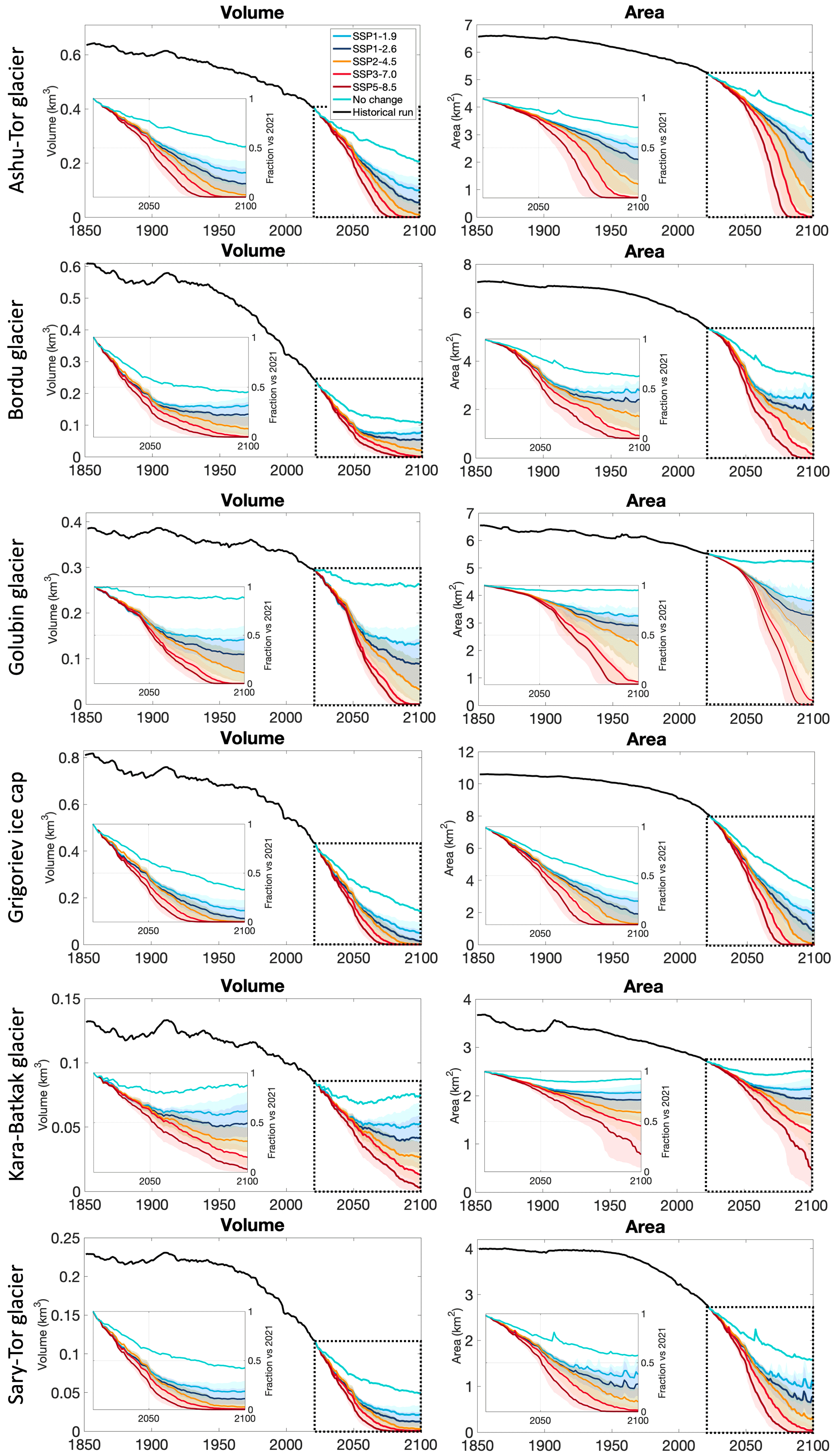
Figure 7Historical and future evolution of the ice volume and area. The insets show the future ice volume and area with respect to 2021.
The pronounced susceptibility of the studied ice masses to climate change can be attributed to the specific climatic conditions in the region. The ice masses in the Tien Shan are spring–summer accumulation types of glaciers (Aizen et al., 2006; Fujita, 2008; Van Tricht et al., 2021b), which means that the accumulation is more sensitive to temperature changes. The air temperature in spring and summer affects both the duration and intensity of melt as well as the type of precipitation, in contrast to glaciers and ice caps with accumulation centred on winter, for which temperatures remain (to date) low enough for solid precipitation. This ensures that warming on winter-type glaciers mainly prolongs and intensifies the melting period without significantly changing accumulation and the average albedo (Aizen et al., 2006; Fujita, 2008). Next to that, in the Tien Shan, the episodic solid precipitation events between May and September preserve the ice from intense melting by increasing the surface albedo, which interrupts the melting season temporarily (Kronenberg et al., 2016; Che et al., 2019). However, increasing temperatures in spring and summer increase melting and reduce the surface albedo, as more precipitation falls in liquid state. The Golubin and Kara-Batkak glaciers, characterized by higher precipitation amounts and, in the case of the former, enhanced winter precipitation, exhibit comparatively lower temperature sensitivity when compared to the other glaciers. Consequently, these glaciers are projected to retain a significant portion of their ice volume under a moderate warming scenario by the end of the century.
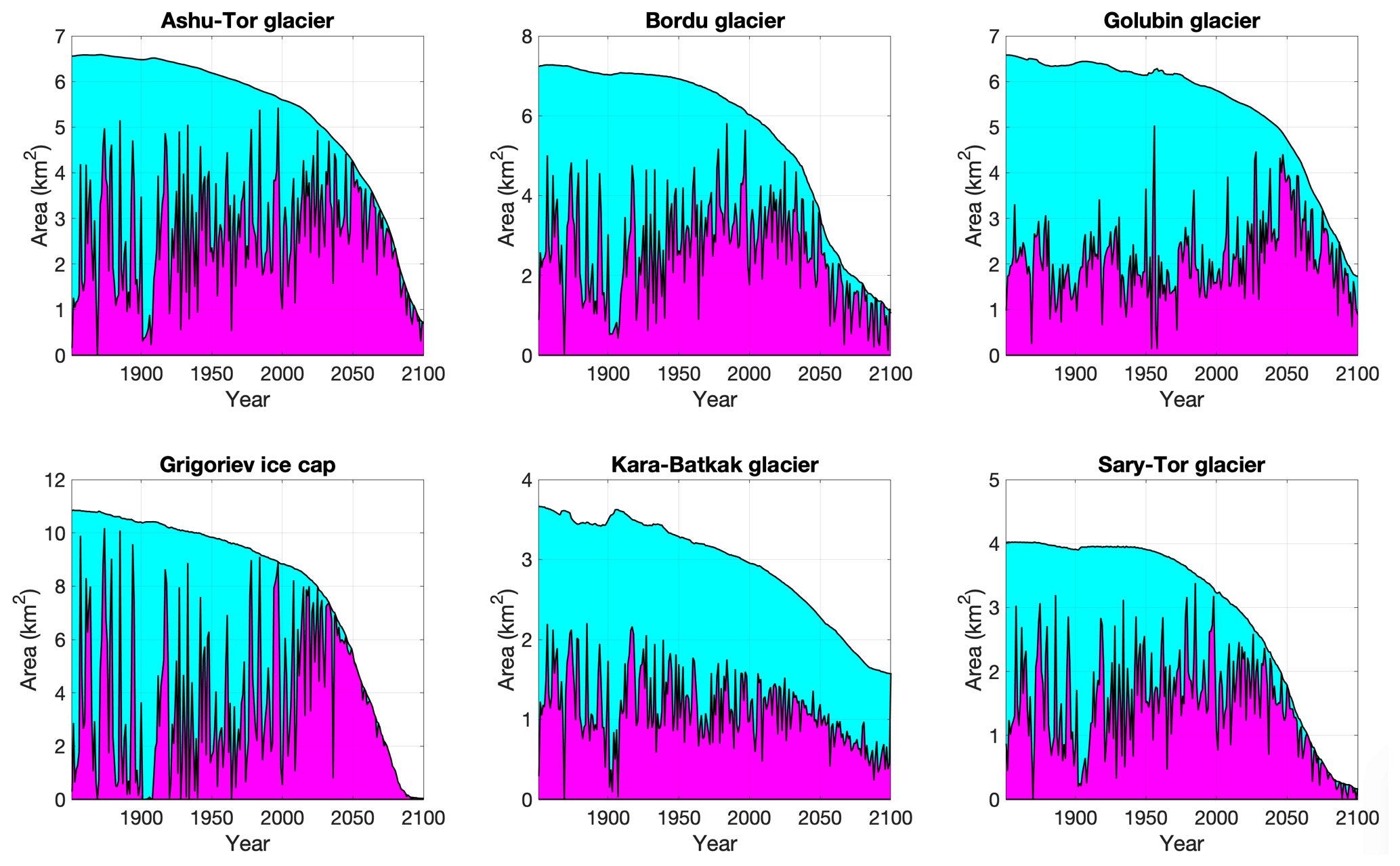
Figure 8Evolution of the accumulation area and the ablation area under SSP2-4.5 for the different ice masses.
5.2 Ice masses in 2100
The ice masses in 2100 are clearly smaller than the present-day geometries in all scenarios (Fig. 9). Nevertheless, it is clear that, depending on the scenario, more or less ice will remain by the end of the 21st century. For the optimistic SSP1-1.9 and SSP1-2.6 scenarios, most ice masses maintain (individual) patches of ice in the upper areas. After the retreat of the ice, the bedrock will appear. As the 2D profiles in the inset already show, there are several (small) depressions in the bedrock that have been scoured by years of ice erosion (Fig. 9). In these bedrock depressions, which will eventually become free of ice, it is very likely that (proglacial) lakes will form (Furian et al., 2022; Compagno et al., 2022). Their formation might accelerate frontal retreat by hydrostatic lifting of the frontal area (Carrivick et al., 2020).
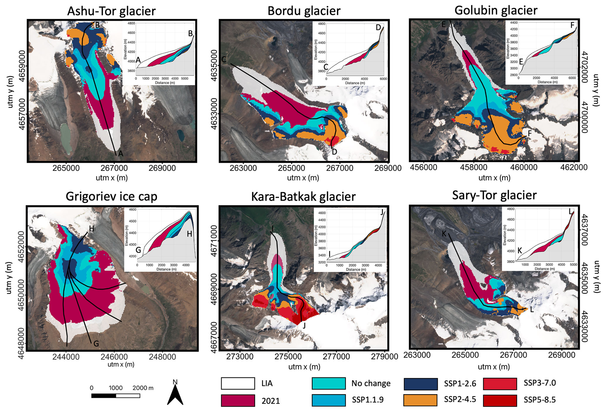
Figure 9Extent of the ice masses at the end of the Little Ice Age (LIA) in 2021 and in 2100 under different climatic scenarios. The inset shows the bedrock and surface profile along the main flowlines, indicated by the black lines on the respective maps. The background satellite images are from Sentinel-2 data acquired in July/August 2021.
5.3 Runoff
The melting of the ice masses in the Tien Shan, which will accelerate in the coming decades (Fig. 7), will lead to profound changes in the runoff. To analyse the projected evolution in the runoff originating from the different ice masses, the annual total runoff is calculated following the approach of Huss and Hock (2018) and Rounce et al. (2020). The runoff (rtot) is defined as all water that leaves the initial (LIA) glacierized area in 1 year. This is computed from the difference between the total precipitation (Ptot) and the mass balance within that area. As such, in the ablation area, the total runoff is the sum of the total precipitation and the glacier meltwater. In the accumulation area and outside the ice masses, it is equal to the total precipitation minus the snow/refrozen water present at the end of the year. Defining the runoff as in Eq. (8) is equivalent to the runoff that would be measured at a fixed gauge at the LIA glacier terminus (Rounce et al., 2020).
The results show that, after an initial increase in the total annual runoff, the continuous retreat of the ice masses leads to a significant decrease in runoff during the second half of the 21st century, except for the Kara-Batkak glacier (Fig. 10). A peak in the total runoff is expected to be reached before or around 2050 in all scenarios. Higher SSP scenarios clearly have a higher peak due to the increased excess glacier meltwater, which corresponds to the additional runoff due to annual glacier net mass loss. However, this peak is shorter, it occurs earlier, and a drastic decrease in total runoff follows afterwards. By contrast, the Kara-Batkak glacier does not exhibit a distinct peak in total runoff.
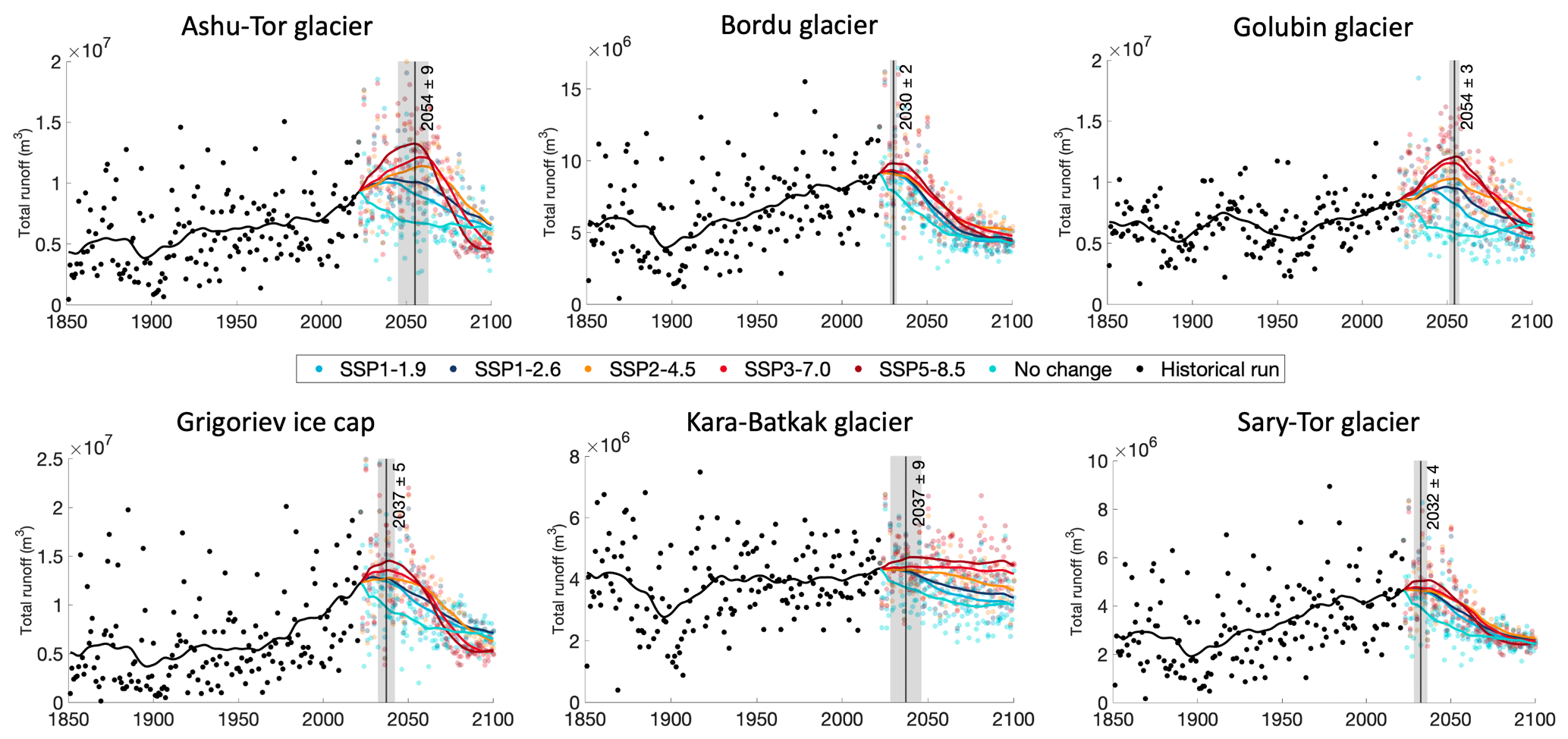
Figure 10Annual total runoff from the initially (Little Ice Age) glacierized area under different climate scenarios. The points represent the modelled total runoff in every year, while the solid line is the 20-year moving average. The indicated year of peak runoff is determined by calculating the average year of the maximum total runoff under SSP1-2.6, SSP2-4.5, SSP3-7.0, and SSP5-8.5, while the grey area corresponds to ± the standard deviation of these years.
Compared to the 2015–2021 average, the total runoff is shown to be reduced on average by 50 % by the end of the 21st century in all scenarios, except for the Golubin and the Kara-Batkak glaciers for which the total runoff remains larger (Fig. 10). It is beyond the focus of this study, but the timing and intensity of runoff during the year also change, with the peak runoff occurring earlier in the year (Rounce et al., 2020). This is because glacial meltwater is a more gradual source of runoff during spring and summer, while runoff from rain/snow is more intense and temporary. During the 21st century, the proportion of ice melt decreases as the ice masses all become significantly smaller in all scenarios. Therefore, the glacial–nival regimes in the region will eventually transform into nival–pluvial regimes with larger year-to-year variability (Braun and Hagg, 2009; Sorg et al., 2012).
6.1 Uncertainty and limitations
The applied methods and the obtained results comprise several uncertainties and limitations which need to be noted. The first set of uncertainties and limitations is related to the observational part of the climatological series, i.e. the temperature and precipitation data used to force the mass balance model from 1850 to 2021. To force the mass balance model, preference was given to local data obtained from meteorological stations in the proximity of the glaciers. However, it should be acknowledged that these local stations may not always accurately capture the conditions prevailing at the glaciers themselves, particularly when there exists a substantial distance between the weather stations and the glaciers. With regard to air temperature, correlations are likely to be reliable over longer distances. Nonetheless, the heterogeneous topography and varied climatological conditions signify that the treatment of precipitation constitutes the primary source of uncertainty in the mass balance calculation. This would, however, also be the case if a reanalysis product were used (De Kok et al., 2020; Barandun and Pohl, 2023). Nevertheless, it is worth noting that our ability to reproduce the present state of ice masses using the local data is demonstrated by the absence of any precipitation or temperature bias for the recent decades.
For the future projections, a multi-model mean was created based on all available GCMs covering the study area. To do this, anomalies with respect to overlapping periods between the GCMs and observations were used and transposed to the future. Although a multi-model mean is beneficial because biases in individual models are less prominent, the use of regional climate models, such as CORDEX, or downscaled products might show additional smaller-scale details and variations (Rana et al., 2020). These small-scale variations, which depend on local elevation and topography, are not included in the forcing of the future but might influence the evolution of the studied ice masses. Nevertheless, a recent study considering glacier evolution in Iceland and Scandinavia pointed out that climate forcing products were only of minor importance for future glacier projections, as opposed to accurate model calibration data at the glacier-specific scale (Compagno et al., 2021). Moreover, Marzeion et al. (2020) demonstrated that the influence of GCM uncertainty in Central Asia typically diminishes during the second half of the century, with the primary driver of uncertainty shifting towards the uncertainty associated with the emission scenarios.
Other limitations are related to the simplicity of the mass balance model, in which different processes such as refreezing and sublimation are not included as independent processes but parameterized as a part of accumulation and ablation. Besides, it must be stated that the mass balance model of the Ashu-Tor glacier is strongly based on the calibrated parameters of nearby glaciers, as direct mass balance measurements were only performed for a limited period in time and for a limited altitudinal extent. This might also be the reason for the mismatch with the geodetic mass balance of Hugonnet et al. (2021). We specifically want to highlight that, given the highly variable precipitation gradient, which is for example evident from the difference of the precipitation gradient between the Bordu glacier and the Grigoriev ice cap, modelled mass balances in the accumulation area of this glacier are characterized by a larger uncertainty.
The uncertainties and limitations in the performance of the ice-flow model are mainly related to the calibration of the enhancement factor and basal sliding parameter, as well as internal ice temperatures. The englacial temperatures were derived using constants for the snow insulation and firn warming to parameterize the surface layer warming as derived in Van Tricht and Huybrechts (2022). However, these constants were only calibrated based on ice temperature data of the Grigoriev ice cap. Nevertheless, validation with GPR measurements showed a close match for the Sary-Tor glacier as well, which increases our confidence that the derived values can be transferred to other glaciers in the region as well. The calibration of the ice flow and basal sliding parameter involved minimizing the differences between the modelled ice thickness and velocities and their corresponding observed values. Nonetheless, these observations also comprise an inherent level of uncertainty, and various combinations produced similar root mean square error (RMSE) values. We obtained values within a comparable range for the difference ice masses. However, the direct calculation of ice temperatures encompasses discrepancies in flow parameters and the existence or non-existence of basal sliding (temperate vs. cold ice over the bed). For Kara-Batkak, we found a larger RMSE between modelled and observed velocities, which was mainly caused by stakes with strong displacement near the margin (Fig. 6). It is possible that our model did not fully resolve glacier dynamics in this part of the glacier with the prescribed parameter combination.
6.2 Evolution of the thermal structure
In our model, we consider the full thermodynamics between 1851 and 2100. Consequently, we also provide an examination of the proportion of temperate ice across the various ice masses from 1851 to 2100 under the SSP2-4.5 scenario (Fig. 11). Our findings reveal distinct thermal regimes across the six ice masses. The Golubin and Kara-Batkak glaciers exhibit a temperate nature due to their slightly lower elevation, resulting in higher mean annual temperatures and larger amounts of precipitation. The greater insulation provided by snow accumulation and a larger volume of refrozen meltwater contributes to enhanced surface warming in these glaciers. In contrast, the Grigoriev ice cap remains consistently cold, as previously demonstrated by Van Tricht and Huybrechts (2022). The Ashu-Tor, Bordu, and Sary-Tor glaciers display a polythermal structure, whereby the proportion of temperate ice gradually diminishes over the course of the 21st century (Fig. 11). This decrease can primarily be attributed to the glacier thinning, retreat to higher elevations, and overall shrinkage. This was also observed for other polythermal glaciers (Willis et al., 2007). Although we anticipate that these changes in the fraction of temperate ice influence glacier dynamics, specifically the transition of lower layers from temperate to cold ice, our study does not delve into a detailed investigation of these dynamics. Nevertheless, we expect a general decrease in velocities when basal sliding becomes smaller or ceases. Future studies could focus on disentangling the influence of considering full thermodynamics on the future evolution.
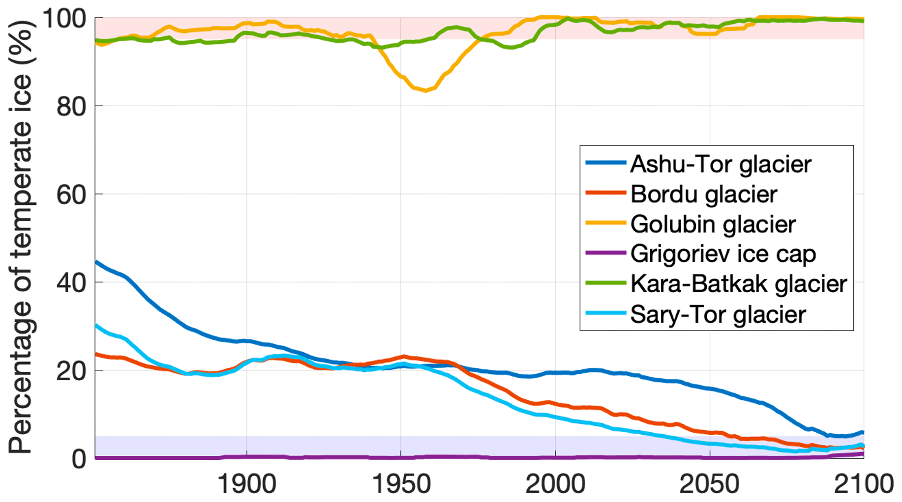
Figure 11Evolution of the percentage of temperate ice for the six ice masses between 1851 and 2100 under SSP2-4.5. The data are smoothed over a period of 10 years. The red area corresponds to >95 % temperate ice, the grey area to 5 %–95 % temperate ice, and the purple area to <5 % temperate ice.
6.3 Heterogeneous response of the different ice masses
According to our research, the six ice masses examined exhibit a heterogeneous response to climate change, which can be attributed to their distinct topographical and climatological settings. Specifically, Kara-Batkak and Golubin were found to retain the largest proportion of their ice volume among all six ice masses. This finding is not surprising, given that these glaciers receive higher amounts of precipitation, particularly in winter and spring, compared to the other four ice masses, where precipitation is lower and concentrated in late spring and the summer months. Consequently, increasing temperatures in the latter lead to a rise in melt and a decline in accumulation. On the other hand, the ice masses' heterogeneous responses can also be attributed to their topographical settings. For instance, the Grigoriev ice cap has a restricted altitudinal range of only 400 m, making it highly vulnerable to climate change. Conversely, the Kara-Batkak glacier spans over 1300 m. Our findings can contribute to the investigation of the heterogeneous impact of climate change on glaciers in the Tien Shan region.
In this study, we modelled the historical and future evolution of six ice masses in the western part of the Tien Shan, High Mountain Asia, using a three-dimensional higher-order ice-flow model coupled to a surface energy mass balance model. The models were calibrated with surface mass balance measurements, length reconstructions, and ice thickness data. Data from tree rings and weather stations in the vicinity of the ice masses served as the meteorological input data for the past. For the Golubin glacier, precipitation data of ERA5 were used as well. Subsequently, different CMIP6 SSP scenarios were considered for the future projections up to 2100, as well as a no change scenario keeping the average climatic conditions of 2001–2021 constant. By implementing minor temperature and/or precipitation biases to account for uncertainties in the mass balance model and discrepancies in the climatic records, specifically for the historical period characterized by less reliable climate information, we were able to successfully reproduce the retreat of the ice masses from the Little Ice Age (1850) to 2021. Validations with geodetic mass balances generally showed a close correspondence. The results highlight a strong increase in the retreat of the ice masses in recent decades.
The projections of the ice masses up to 2100 reveal that, under all climate scenarios, the ice masses become significantly smaller. Under the SSP5-8.5 scenario, most of the ice masses disappear altogether, except for the Kara-Batkak glacier, which appears to be able to maintain small ice patches at the highest elevations. The Grigoriev ice cap shows the strongest climate sensitivity, disappearing in almost every climate scenario. This could be explained by the small ice cap instability, with the equilibrium line rising above the top of the ice cap even in the most optimal climate scenario. Besides, the studied ice masses appear to be particularly sensitive to climate change because the accumulation is centred around spring and early summer. Hence, temperature rises in these seasons not only amplify melting but also reduce the solid part of the precipitation and the average albedo. Projections of the total annual runoff from the LIA glacierized catchment show that the peak water will be reached before the middle of the 21st century and that the intensity of this peak depends on the climate scenario, with a higher warming scenario having a larger peak.
The availability of a comprehensive set of accurate direct measurements allowed us to study in detail a sample of six ice masses in the Tien Shan. The different geometries and climatic settings of the ice bodies additionally permitted analysis of why certain ice masses disappear faster (e.g. the Grigoriev ice cap) or can survive (e.g. the Kara-Batkak glacier). As a next step, it would be interesting to compare the results of this study to the outcomes of simpler regional models providing ice volume evolutions for all glaciers in the study area. This can give an insight into the added value of using higher-order models and a more detailed representation of the thermal regime, and it will allow one to assess the value and quality of larger-scale models that are required for regional studies of ice volume evolution.
Information and specific details about the model code will be specified on request to Lander Van Tricht.
Research data are provided through an online public repository, accessible via https://doi.org/10.5281/zenodo.8425516 (Van Tricht, 2023). Additional data can be requested from Lander Van Tricht.
LVT collected the input data, prepared the climate scenarios, performed the experiments, and wrote the paper. PH provided the model code, gave guidance on implementing the research and interpreting the results, and assisted with writing the paper.
The contact author has declared that neither of the authors has any competing interests.
Publisher’s note: Copernicus Publications remains neutral with regard to jurisdictional claims in published maps and institutional affiliations.
The authors would like to thank everyone who contributed to the fieldwork to carry out the ice thickness measurements and the drone surveys. We would also like to specifically thank Oleg Rybak and Rysbek Satylkanov for assisting with and organizing the fieldwork. We thank Victor Popovnin for providing the mass balance data. We are also grateful to the Kumtor Gold Company for allowing us to perform glacier measurements on their concession.
Lander Van Tricht holds a PhD fellowship from the Research Foundation – Flanders (FWO-Vlaanderen) and is affiliated with the Vrije Universiteit Brussel (VUB). The logistics for fieldwork on the glaciers were mainly organized and funded by the Tien Shan High Mountain Research Center and the Kumtor Gold Company.
This paper was edited by Tobias Sauter and reviewed by Adrien Gilbert, Julia Eis, and one anonymous referee.
Aizen, V. B., Maksimov, N. V., and Solodov, P. A.: Dynamiealednika Grolubina za poslednie 20 let [Dynamic of the Golubina Glacier for the 20 last years], Trudi Central'no-Asiatskogo Regional'nogo Naucho-Issledovatel'skogo Instituta [Works of Central Asian Regional Institute of Science Investigations, Tashkent], 91, 172, 1983 (in Russian).
Aizen, V. B., Aizen, E. M., and Melack, J. M.: Climate, Snow Cover, Glaciers, and Runoff in the Tien Shan, Central Asia, J. Am. Water Resour. As., 31, 1113–1129, https://doi.org/10.1111/j.1752-1688.1995.tb03426.x, 1995.
Aizen, V. B., Kuzmichenok, V., Surazakov, A., and Aizen, E. M.: Glacier changes in the central and northern Tien Shan during the last 140 years based on surface and remote-sensing data, Ann. Glaciol., 43, 202–213, https://doi.org/10.3189/172756406781812465, 2006.
Aizen, V. B., Kuzmichenok, V. A., Surazakov, A. B., and Aizen, E. M.: Glacier Changes in the Tien Shan as Determined from Topographic and Remotely Sensed Data, Global Planet. Change, 56, 328–340, https://doi.org/10.1016/j.gloplacha.2006.07.016, 2007.
Arkhipov, S. M., Mikhalenko, V. N., Kunakhovich, M. G., Dikikh, A. N., and Nagornov, O. V.: Termich eskii rezhim, usloviia l'doobrazovaniia i akkumulyatsiia na ladnike Grigor'eva (Tyan'-Shan') v 1962–2001 gg. [Thermal regime, ice types and accumulation in Grigoriev Glacier, Tien Shan, 1962–2001], Mater. Glyatsiol. Issled., 96, 77–83, 2004 (in Russian with English summary).
Azisov, E., Hoelzle, M., Vorogushyn, S., Saks, T., Usubaliev, R., Esenaman uulu, M., and Barandun, M.: Reconstructed Centennial Mass Balance Change for Golubin Glacier, Northern Tien Shan, Atmosphere, 13, 954, https://doi.org/10.3390/atmos13060954, 2022.
Barandun, M. and Pohl, E.: Central Asia's spatiotemporal glacier response ambiguity due to data inconsistencies and regional simplifications, The Cryosphere, 17, 1343–1371, https://doi.org/10.5194/tc-17-1343-2023, 2023.
Barandun, M., Huss, M., Usubaliev, R., Azisov, E., Berthier, E., Kääb, A., Bolch, T., and Hoelzle, M.: Multi-decadal mass balance series of three Kyrgyz glaciers inferred from modelling constrained with repeated snow line observations, The Cryosphere, 12, 1899–1919, https://doi.org/10.5194/tc-12-1899-2018, 2018.
Barandun, M., Pohl, E., Naegeli, K., McNabb, R., Huss, M., Berthier, E., Saks, T., and Hoelzle, M.: Hot spots of glacier mass balance variability in Central Asia, Geophys. Res. Lett., 48, e2020GL092084, https://doi.org/10.1029/2020GL092084, 2021.
Blomdin, R., Stroeven, A. P., Harbor, J. M., Lifton, N. A., Heyman, J., Gribenski, N., Petrakov, D. A., Caffee, M. W., Ivanov, M. N., Hättestrand, C., Rogozhina, I., and Usubaliev R.: Evaluating the timing of former glacier expansions in the Tian Shan: A key step towards robust spatial correlations, Quaternary Sci. Rev., 153, 78–96, https://doi.org/10.1016/j.quascirev.2016.07.029, 2016.
Bolch, T.: Glacier area and mass changes since 1964 in the Ala Archa Valley, Kyrgyz Ala-Too, northern Tien Shan, Led i Sneg, 129, 28–39, https://doi.org/10.5167/uzh-117189, 2015,
Braun, L. N. and Hagg, W.: Present and future impact of snow cover and glaciers on runoff from mountain regions – comparison between Alps and Tien Shan, in: IHP-HWRP-Berichte, 8, 36–43, https://doi.org/10.5282/ubm/epub.13807, 2009.
Brun, F., Berthier, E., Wagnon, P., Kääb, A., and Treichler, D.: A spatially resolved estimate of High Mountain Asia glacier mass balances from 2000 to 2016, Nat. Geosci., 10, 668–673, https://doi.org/10.1038/ngeo2999, 2017.
Carrivick, J. L., Tweed, F. S., Sutherland, J. L., and Mallalieu, J.: Toward Numerical Modeling of Interactions between Ice-Marginal Proglacial Lakes and Glaciers, Front. Earth Sci., 8, 577068, https://doi.org/10.3389/feart.2020.577068, 2020.
Che, Y., Zhang, M., Li, Z., Wei, Y., Nan, Z., Li, H., Wang, S., and Su, B.: Energy balance model of mass balance and its sensitivity to meteorological variability on Urumqi River Glacier No.1 in the Chinese Tien Shan, Sci. Rep., 9, 13958, https://doi.org/10.1038/s41598-019-50398-4, 2019.
Christian, J. E., Koutnik, M., and Roe, G.: Committed retreat: Controls on glacier disequilibrium in a warming climate, J. Glaciol., 64, 675–688, https://doi.org/10.1017/jog.2018.57, 2018.
Compagno, L., Zekollari, H., Huss, M., and Farinotti, D.: Limited impact of climate forcing products on future glacier evolution in Scandinavia and Iceland, J. Glaciol., 67, 727–743, https://doi.org/10.1017/jog.2021.24, 2021.
Compagno, L., Huss, M., Zekollari, H., and Farinotti, D.: Future growth and decline of high mountain Asia's ice-dammed lakes and associated risk, Commun. Earth Environ., 3, 191, https://doi.org/10.1038/s43247-022-00520-8, 2022.
de Kok, R. J., Kraaijenbrink, P. D. A., Tuinenburg, O. A., Bonekamp, P. N. J., and Immerzeel, W. W.: Towards understanding the pattern of glacier mass balances in High Mountain Asia using regional climatic modelling, The Cryosphere, 14, 3215–3234, https://doi.org/10.5194/tc-14-3215-2020, 2020.
Dikikh, A. N.: Temperature regime of flat-top glaciers (using Grigoriev as an Example) – Glyatsiol, Issledovaniya na Tyan-Shane, Frunze, N. 11, 32–35, 1965 (in Russian).
Dyurgerov, M. B.: Glacier mass balance and regime: data of measurements and analysis, University of Colorado Institute of Arctic and Alpine Research Occasional Paper 55, Boulder, http://instaar.colorado.edu/other/occ_papers.html (last access: 17 October 2022), 2002.
Eyring, V., Bony, S., Meehl, G. A., Senior, C. A., Stevens, B., Stouffer, R. J., and Taylor, K. E.: Overview of the Coupled Model Intercomparison Project Phase 6 (CMIP6) experimental design and organization, Geosci. Model Dev., 9, 1937–1958, https://doi.org/10.5194/gmd-9-1937-2016, 2016.
Farinotti, D., Longuevergne, L., Moholdt, G., Duethmann, D., Mölg, T., Bolch, T., and Vorogushyn, S.: Güntner, A. Substantial glacier mass loss in the Tien Shan over the past 50 years, Nat. Geosci., 8, 716–722, https://doi.org/10.1038/ngeo2513, 2015.
Fujita, K.: Influence of precipitation seasonality on glacier mass balance and its sensitivity to climate change, Ann. Glaciol., 48, 88–92, https://doi.org/10.3189/172756408784700824, 2008.
Fujita, K., Takeuchi, N., Nikitin, S. A., Surazakov, A. B., Okamoto, S., Aizen, V. B., and Kubota, J.: Favorable climatic regime for maintaining the present-day geometry of the Gregoriev Glacier, Inner Tien Shan, The Cryosphere, 5, 539–549, https://doi.org/10.5194/tc-5-539-2011, 2011.
Furian, W., Maussion, F., and Schneider, C.: Projected 21st-century glacial lake evolution in High Mountain Asia, Front. Earth Sci., 10, 821798, https://doi.org/10.3389/feart.2022.821798, 2022.
Fürst, J. J., Rybak, O., Goelzer, H., De Smedt, B., de Groen, P., and Huybrechts, P.: Improved convergence and stability properties in a three-dimensional higher-order ice sheet model, Geosci. Model Dev., 4, 1133–1149, https://doi.org/10.5194/gmd-4-1133-2011, 2011.
Fürst, J. J., Goelzer, H., and Huybrechts, P.: Effect of higher-order stress gradients on the centennial mass evolution of the Greenland ice sheet, The Cryosphere, 7, 183–199, https://doi.org/10.5194/tc-7-183-2013, 2013.
Gan, R., Luo, L., Zuo, Q., and Sun, L.: Effects of projected climate change on the glacier and runoff generation in the Naryn River Basin, Central Asia, J. Hydrol., 523, 240–251, https://doi.org/10.1016/j.jhydrol.2015.01.057, 2015.
Goerlich, F., Bolch, T., Mukherjee, K., and Pieczonka, T.: Glacier Mass Loss during the 1960s and 1970s in the Ak-Shirak Range (Kyrgyzstan) from Multiple Stereoscopic Corona and Hexagon Imagery, Remote Sensing, 9, 275, https://doi.org/10.3390/rs9030275, 2017.
Hagg, W., Braun, L. N., Weber, M., and Becht, M.: Runoff modelling in glacierized central Asian catchments for present-day and future climate, Hydrol. Res., 37, 93–105, https://doi.org/10.2166/nh.2006.0008, 2006.
Hausfather, Z., Marvel, K., Schmidt, G. A., Nielsen-Gammon, J. W., and Zelinka, M.: Climate simulations: Recognize the “hot model” problem, Nature, 605, 26–29, https://doi.org/10.1038/d41586-022-01192-2, 2022.
Hoelzle, M., Azisov, E., Barandun, M., Huss, M., Farinotti, D., Gafurov, A., Hagg, W., Kenzhebaev, R., Kronenberg, M., Machguth, H., Merkushkin, A., Moldobekov, B., Petrov, M., Saks, T., Salzmann, N., Schöne, T., Tarasov, Y., Usubaliev, R., Vorogushyn, S., Yakovlev, A., and Zemp, M.: Re-establishing glacier monitoring in Kyrgyzstan and Uzbekistan, Central Asia, Geosci. Instrum. Method. Data Syst., 6, 397–418, https://doi.org/10.5194/gi-6-397-2017, 2017.
Hoelzle, M., Barandun, M., Bolch, T., Fiddes, J., Gafurov, A., Muccione, V., Saks, T., and Shahgedanova, M.: The status and role of the alpine cryosphere in Central Asia, in: The Aral Sea Basin, Taylor & Francis, https://doi.org/10.4324/9780429436475-8, 2019.
Hugonnet, R., McNabb, R., Berthier, E., Menounos, B., Nuth, C., Girod, L., Farinotti, D., Huss, M., Dussaillant, I., Brun, F., and Kääb, A.: Accelerated global glacier mass loss in the early twenty-first century, Nature, 592, 726–731, https://doi.org/10.1038/s41586-021-03436-z, 2021.
Huss, M. and Hock, R: Global-scale hydrological response to future glacier mass loss, Nat. Clim. Change, 8, 135–140, https://doi.org/10.1038/s41558-017-0049-x, 2018.
Hutter, K.: Theoretical glaciology, vol. 1, Reidel Publ. Co, Dordrecht, https://doi.org/10.1007/978-94-015-1167-4_1, 1983.
Huybrechts, P.: A 3-D model for the Antarctic ice sheet: a sensitivity study on the glacial-interglacial contrast, Clim. Dynam., 5, 79–92, https://doi.org/10.1007/BF00207423, 1990.
Immerzeel, W. W., Van Beek, L. P., and Bierkens, M. F.: Climate change will affect the Asian water towers, Science, 328, 1382–1385, https://doi.org/10.1126/science.1183188, 2010.
Jóhannesson, T., Raymond, C., and Waddington, E.: Time–Scale for Adjustment of Glaciers to Changes in Mass Balance, J. Glaciol., 35, 355–369, https://doi.org/10.3189/S002214300000928X, 1989.
Jouvet, G., Huss, M., Funk, M., and Blatter, H.: Modelling the retreat of Grosser Aletschgletscher, Switzerland, in a changing climate, J. Glaciol., 57, 1033–1045, https://doi.org/10.3189/002214311798843359, 2011.
Kraaijenbrink, P., Bierkens, M., Lutz, A., and Immerzeel W. W.: Impact of a global temperature rise of 1.5 degrees Celsius on Asia's glaciers, Nature, 549, 257–260, https://doi.org/10.1038/nature23878, 2017.
Kronenberg, M., Barandun, M., Hoelzle, M., Huss, M., Farinotti, D., Azisov, E., Usubaliev, R., Gafurov, A., Petrakov, D., and Kääb, A.: Mass-balance reconstruction for Glacier No. 354, Tien Shan, from 2003 to 2014, Ann. Glaciol., 57, 92–102, https://doi.org/10.3189/2016AoG71A032, 2016.
Kutuzov, S. and Shahgedanova, M.: Glacier retreat and climatic variability in the eastern Terskey–Alatoo, inner Tien Shan between the middle of the 19th century and beginning of the 21st century, Global Planet. Change, 69, 59–70, https://doi.org/10.1016/j.gloplacha.2009.07.001, 2009.
Li, Y., Lu, X., and Li, Y.: A Review on the Little Ice Age and Factors to Glacier Changes in the Tian Shan, Central Asia, in: Glaciers Evolution in a Changing World, IntechOpen, Vienna, Austria, https://doi.org/10.5772/intechopen.70044, 2017.
Marzeion, B., Hock, R., Anderson, B., Bliss, A., Champollion, N., Fujita, K., Huss, M., Immerzeel, W., Kraaijenbrink, P., Malles, J.-H., Maussion, F., Radíc, V., Rounce, D. R., Sakai, A., Shannon, S., van de Wal, R., and Zekollari, H.: Partitioning the uncertainty of ensemble projections of global glacier mass change, Earth's Future, 8, e2019EF001470, https://doi.org/10.1029/2019EF001470, 2020.
Mikhalenko, V. N.: Osobennosti massoobmena lednikov ploskikh vershin vnutrennego Tyan'-Shanya [Peculiarities of the mass exchange of flat summit glaciers of interior Tyan'-Shan'], Materialy Glyatsiologicheskikh Issledovaniy, 65, 86–92, 1989 (in Russian).
Narama, C., Daiyrov, M., Duishonakunov, M., Tadono, T., Sato, H., Kääb, A., Ukita, J., and Abdrakhmatov, K.: Large drainages from short-lived glacial lakes in the Teskey Range, Tien Shan Mountains, Central Asia, Nat. Hazards Earth Syst. Sci., 18, 983–995, https://doi.org/10.5194/nhess-18-983-2018, 2018.
Pattyn, F.: A new three-dimensional higher-order thermomechanical ice sheet model: Basic sensitivity, ice stream development, and iceflow across subglacial lakes, J. Geophys. Res., 108, B82382, https://doi.org/10.1029/2002JB002329, 2003.
Petrakov, D. A., Lavrientiev, I. I., Kovalenko, N. V., and Usubaliev, R. A.: Ice thickness, volume and modern change of the Sary-Tor Glacier area (Ak-Shyirak Massif, Inner Tian Shan), Earth's Cryosphere, 18, 91–100, 2014.
Pieczonka, T. and Bolch, T.: Region-wide Glacier Mass Budgets and Area Changes for the Central Tien Shan between ∼ 1975 and 1999 Using Hexagon KH-9 Imagery, Global Planet. Change, 128, 1–13, https://doi.org/10.1016/j.gloplacha.2014.11.014, 2015.
Pritchard, H. D.: Asia's shrinking glaciers protect large populations from drought stress, Nature, 569, 649–654, https://doi.org/10.1038/s41586-019-1240-1, 2019.
Rana, A., Nikulin, G., Kjellström, E. Strandberg, G., Kupiainen, M., Hansson, U., and Kolax, M.: Contrasting regional and global climate simulations over South Asia, Clim. Dynam., 54, 2883–2901, https://doi.org/10.1007/s00382-020-05146-0, 2020.
RGI Consortium: Randolph Glacier Inventory – A Dataset of Global Glacier Outlines, Version 6, NSIDC: National Snow and Ice Data Center Boulder, Colorado USA [data set], https://doi.org/10.7265/4m1f-gd79, 2017.
Rounce, D. R., Hock, R., and Shean, D. E.: Glacier Mass Change in High Mountain Asia Through 2100 Using the Open-Source Python Glacier Evolution Model (PyGEM), Front. Earth Sci., 7, 331, https://doi.org/10.3389/feart.2019.00331, 2020.
Satylkanov, R.: Ablation of Ice and Snow of Kara-Batkak Glacier and its Impact on River Flow, Journal of Climate Change, 4, 1–14, https://doi.org/10.3233/jcc-180009, 2018.
Savoskul, O. S. and Solomina, O. N.: Late-Holocene glacier variations in the frontal and inner ranges of Tian Shan, central Asia, Holocene, 6, 25–35, https://doi.org/10.1177/095968369600600104, 1996.
Shahgedanova, M., Afzal, M., Hagg, W., Kapitsa, V., Kasatkin, N., Mayr, E., Rybak, O., Saidaliyeva, Z., Severskiy, I., Usmanova, Z., Wade, A., Yaitskaya, N., and Zhumabayev, D.: Emptying Water Towers? Impacts of Future Climate and Glacier Change on River Discharge in the Northern Tien Shan, Central Asia, Water, 12, 627, https://doi.org/10.3390/w12030627, 2020.
Shean, D.E., Bhushan, S., Montesano, P., Rounce, D. R., Arendt, A., and Osmanoglu, B.: A systematic, regional assessment of high mountain Asia glacier mass balance, Front. Earth Sci., 7, 363, https://doi.org/10.3389/feart.2019.00363, 2020.
Solomina, O., Barry, R., and Bodnya, M.: The Retreat of Tien Shan Glaciers (Kyrgyzstan) since the Little Ice Age Estimated from Aerial Photographs, Lichenometric and Historical Data, Geogr. Ann. A, 86, 205–215, https://doi.org/10.1111/j.0435-3676.2004.00225.x, 2004.
Solomina, O., Maximova, O., and Cook, E.: Picea Schrenkiana Ring Width and Density at the Upper and Lower Tree Limits in the Tien Shan Mts (Kyrgyz Republic) as a Source of Paleoclimatic Information, Geogr. Environ. Sustain., 7, 66–79, https://doi.org/10.24057/2071-9388-2014-7-1-66-79, 2014.
Sorg, A., Bolch, T., Stoffel, M., Solomina, O., and Beniston, M.: Climate change impacts on glaciers and runoff in Tien Shan (Central Asia), Nat. Clim. Change, 2, 725–731, https://doi.org/10.1038/nclimate1592, 2012.
Takeuchi, N., Fujita, K., Aizen, V. B., Narama, C., Yokoyama, Y., Okamoto, S., Naoki, K., and Kubota, J.: The disappearance of glaciers in the Tien Shan Mountains in Central Asia at the end of Pleistocene, Quaternary Sci. Rev., 103, 26–33, https://doi.org/10.1016/j.quascirev.2014.09.006, 2014.
Thompson, L. G., Mosley-Thompson, E., Davis, M., Lin, P. N., Yao, T., Dyurgerov, M., and Dai, J.: Recent warming: ice core evidence from tropical ice cores with emphasis on Central Asia, Global Planet. Change, 7, 145–156, https://doi.org/10.1016/0921-8181(93)90046-Q, 1993.
Van Tricht, L.: LanderVT/Modelling_glaciers_TienShan: Modelling_glaciers_TienShan, Zenodo [data set], https://doi.org/10.5281/zenodo.8425516, 2023.
Van Tricht, L. and Huybrechts, P.: Thermal regime of the Grigoriev ice cap and the Sary-Tor glacier in the inner Tien Shan, Kyrgyzstan, The Cryosphere, 16, 4513–4535, https://doi.org/10.5194/tc-16-4513-2022, 2022.
Van Tricht, L., Huybrechts, P., Van Breedam, J., Fürst, J., Rybak, O., Satylkanov, R., Ermenbaiev B., Popovnin V., Neyns, R., Paice C. M., and Malz, P.: Measuring and inferring the ice thickness distribution of four glaciers in the Tien Shan, Kyrgyzstan, J. Glaciol., 67, 269–286, https://doi.org/10.1017/jog.2020.104, 2021a.
Van Tricht, L., Paice, C. M., Rybak, O., Satylkanov, R., Popovnin, V., Solomina, O., and Huybrechts, P.: Reconstruction of the Historical (1750–2020) Mass Balance of Bordu, Kara-Batkak and Sary-Tor Glaciers in the Inner Tien Shan, Kyrgyzstan, Front. Earth Sci., 9, 734802, https://doi.org/10.3389/feart.2021.734802, 2021b.
Van Tricht, L., Huybrechts, P., Van Breedam, J., Vanhulle, A., Van Oost, K., and Zekollari, H.: Estimating surface mass balance patterns from unoccupied aerial vehicle measurements in the ablation area of the Morteratsch–Pers glacier complex (Switzerland), The Cryosphere, 15, 4445–4464, https://doi.org/10.5194/tc-15-4445-2021, 2021c.
Van Tricht, L., Paice, C. M., Rybak, O., and Huybrechts, P.: Brief communication: Measuring and modelling the ice thickness of the Grigoriev ice cap (Kyrgyzstan) and comparison with global datasets, The Cryosphere, 17, 4315–4323, https://doi.org/10.5194/tc-17-4315-2023, 2023.
Venukov, M. I.: Ocherki Zailiiskogo kraya i Prichuiskoi strain [Essays of Zailiiski region and Prichuiskii country], Izv. Russ. Geograf. Obshch., Rossiiskaya Akademiya Nauk, 4, 35–61, 1861.
Willis, I. C., Rippin, D. M., and Kohler, J.: Thermal regime changes of the polythermal Midre Lovénbreen, Svalbard. In The Dynamics and Mass Budget of Arctic Glaciers (Extended Abstracts), Workshop and GLACIODYN (IPY) Meeting, 15–18 January 2007, Pontresina, Italy, Institute for Marine and Atmospheric Research, Utrecht University (IMAU), Utrecht, 130–133, 2007.
Zekollari, H. and Huybrechts, P.: On the climate–geometry imbalance, response time and volume–area scaling of an alpine glacier: insights from a 3-D flow model applied to Vadret da Morteratsch, Switzerland, Ann. Glaciol., 56, 51–62, https://doi.org/10.3189/2015AoG70A921, 2015.
Zekollari, H., Huybrechts, P., Fürst, J. J., Rybak, O., and Eisen, O.: Calibration of a higher-order 3-D ice-flow model of the Morteratsch glacier complex, Engadin, Switzerland, Ann. Glaciol., 54, 343–351, https://doi.org/10.3189/2013AoG63A434, 2013.
Zekollari, H., Fürst, J., and Huybrechts, P.: Modelling the evolution of Vadret da Morteratsch, Switzerland, since the Little Ice Age and into the future, J. Glaciol., 60, 1155–1168, https://doi.org/10.3189/2014JoG14J053, 2014.
Zekollari, H., Huybrechts, P., Noël, B., van de Berg, W. J., and van den Broeke, M. R.: Sensitivity, stability and future evolution of the world's northernmost ice cap, Hans Tausen Iskappe (Greenland), The Cryosphere, 11, 805–825, https://doi.org/10.5194/tc-11-805-2017, 2017.
- Abstract
- Introduction
- Location and climate
- Method and models
- Dynamical calibration and historical reconstruction
- Future evolution of the ice masses
- Discussion and outlook
- Conclusion
- Code availability
- Data availability
- Author contributions
- Competing interests
- Disclaimer
- Acknowledgements
- Financial support
- Review statement
- References