the Creative Commons Attribution 4.0 License.
the Creative Commons Attribution 4.0 License.
 | 06 Oct 2023
A framework for time-dependent ice sheet uncertainty quantification, applied to three West Antarctic ice streams
Daniel Goldberg
James R. Maddison
Joe Todd
Ice sheet models are the main tool to generate forecasts of ice sheet mass loss, a significant contributor to sea level rise; thus, knowing the likelihood of such projections is of critical societal importance. However, to capture the complete range of possible projections of mass loss, ice sheet models need efficient methods to quantify the forecast uncertainty. Uncertainties originate from the model structure, from the climate and ocean forcing used to run the model, and from model calibration. Here we quantify the latter, applying an error propagation framework to a realistic setting in West Antarctica. As in many other ice sheet modelling studies we use a control method to calibrate grid-scale flow parameters (parameters describing the basal drag and ice stiffness) with remotely sensed observations. Yet our framework augments the control method with a Hessian-based Bayesian approach that estimates the posterior covariance of the inverted parameters. This enables us to quantify the impact of the calibration uncertainty on forecasts of sea level rise contribution or volume above flotation (VAF) due to the choice of different regularization strengths (prior strengths), sliding laws, and velocity inputs. We find that by choosing different satellite ice velocity products our model leads to different estimates of VAF after 40 years. We use this difference in model output to quantify the variance that projections of VAF are expected to have after 40 years and identify prior strengths that can reproduce that variability. We demonstrate that if we use prior strengths suggested by L-curve analysis, as is typically done in ice sheet calibration studies, our uncertainty quantification is not able to reproduce that same variability. The regularization suggested by the L curves is too strong, and thus propagating the observational error through to VAF uncertainties under this choice of prior leads to errors that are smaller than those suggested by our two-member “sample” of observed velocity fields.
- Article
(10283 KB) - Full-text XML
- BibTeX
- EndNote


Ice sheet models are important tools not only for generating knowledge, but also for operational forecasts. In this way, they are analogous to weather models and oceanographic models and have emerged as the de facto standard for generating projections of ice sheet contribution to sea level rise. However, quantifying the uncertainty in forecasts produced by these models remains one of the most challenging goals of scientific inquiry (Aschwanden et al., 2021). Here, we seek to characterize the uncertainty in model projections of marine ice sheet loss which arises from calibration with data.
The paradigm of ice sheet projection is the calibration of the model parameters with observations (via control methods; e.g. Macayeal, 1992), followed by running of the calibrated model forward in time forced by future ocean and climate scenarios. The process is uncertain due to (i) model and structural uncertainty (i.e. uncertainty in the formulation of the model and its ability to represent the physics of the system), (ii) uncertainty in external forcing (e.g. ocean melting of ice shelves), and (iii) calibration uncertainty (i.e. the uncertainty in calibrated parameters, sometimes referred to as parametric uncertainty). In this study we use control methods and a Bayesian inference approach to characterize (iii). The Bayesian framework computes posterior information given the assumed model and external forcing. We do not attempt to quantify (i) and (ii), but we discuss how these uncertainties can be quantified and incorporated into our error propagation framework.
The use of control methods (“inverse methods”) in ice sheet modelling dates back to Macayeal (1992). Since then, their use in estimating basal and internal conditions (hidden properties) of glaciers and ice sheets from measured surface velocities has become widespread (e.g. Sergienko et al., 2008; Morlighem et al., 2010; Cornford et al., 2015; Hill et al., 2021, to name a few). This is mostly due to the ability of these methods to perform large-scale inversions via the minimization of a cost function, thus allowing a better representation of basal and rheological conditions to which the ice flow is sensitive (Barnes et al., 2021). However, these data assimilation techniques may not be well posed (Petra et al., 2014) and a unique solution is never guaranteed, regardless of the control method used (Barnes et al., 2021). Control methods have regularization terms which need to be chosen in order to impose smoothness on the inverted parameters (Koziol et al., 2021). In many studies, the strength of the regularization is determined heuristically through L-curve analysis (Gillet-Chaulet et al., 2012; Barnes et al., 2021). Additionally, control methods do not provide calibration uncertainty. They can be interpreted as methods that return only the mode of a posterior probability density function (PDF) of the inverted model parameters, which does not fully characterize calibration uncertainty (Koziol et al., 2021), nor does it propagate the observational uncertainty onto projections of sea level rise.
Previous works attempted to quantify uncertainty by considering the forcing uncertainty (Tsai et al., 2017; Robel et al., 2019; Levermann et al., 2020) or structural uncertainty (Hill et al., 2021). Others considered calibration uncertainty (Isaac et al., 2015; DeConto and Pollard, 2016; Brinkerhoff et al., 2021; Brinkerhoff, 2022) but used low-dimensional parameter sets (i.e. smaller than ∼20) to describe the ice rheology and basal friction. Here we carry out the first assessment of calibration uncertainty using a time-dependent marine ice sheet model (FEniCS_ice, Koziol et al., 2021) in which the calibration of the ice dynamic parameters scales with the dimension of the numerical grid – i.e. we calibrate each parameter for every element in our mesh of approximately 100 000 unknowns (see Fig. 1).
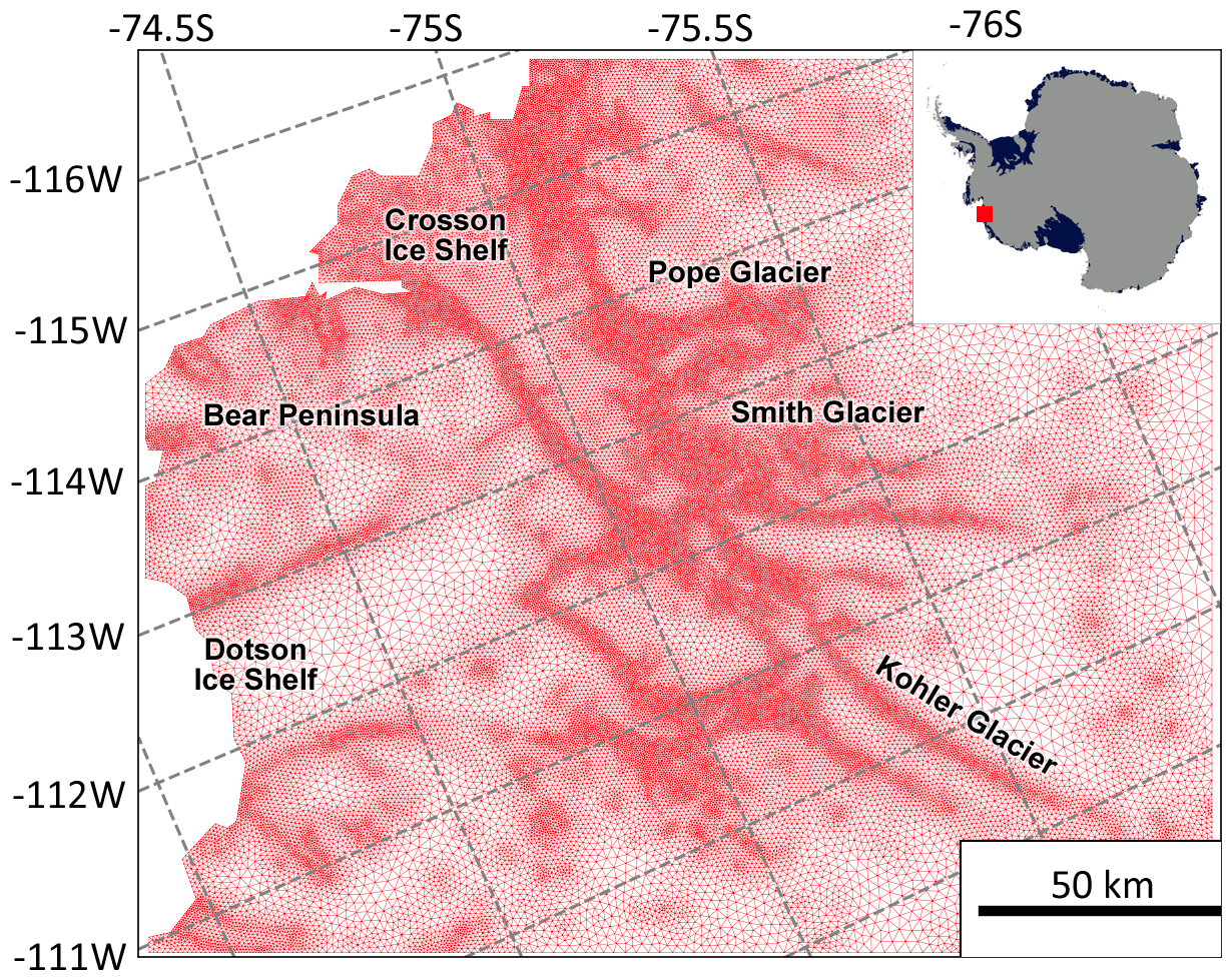
Figure 1Variable-resolution mesh of the study domain. The resolution depends on observed strain rates derived by using satellite velocity data (MEaSUREs v1.0 1996–2012, Rignot et al., 2014) and BedMachine Antarctica v2.0 (Morlighem et al., 2020). The boundaries to the east and south are entirely ice–ice boundaries, whereas the north and west feature calving fronts where ice meets the ocean.
We deal with the problem of estimating the uncertainty in the calibrated parameters (or in the solution of our infinite-dimensional inverse problem) with the framework of Bayesian inference (Tarantola, 2005; Stuart, 2010), in which prior knowledge is “updated” with observational evidence (Koziol et al., 2021). Given satellite ice velocity observations (and their uncertainty), a forward model that maps parameters to observations (e.g. FEniCS_ice), and a prior probability density on model parameters that encodes any prior knowledge or assumptions regarding the parameters (e.g. prior covariance of the ice stiffness parameter in Glen's ice flow law; Glen and Perutz, 1955; Pattyn, 2010), we find the posterior probability density of the parameters conditioned on the observational data. This posterior probability density function (PDF) is defined as the Bayesian solution of our ice sheet inverse problem (Petra et al., 2014). A standard approach to characterize this posterior PDF is based on sampling via state-of-the-art Markov chain Monte Carlo (MCMC) methods. Yet the use of conventional MCMC approaches becomes intractable and prohibitive due to computational expense for large-scale ice sheet inverse problems where we would need a very large number of realizations of the time-dependent nonlinear Stokes equation (Isaac et al., 2015; Koziol et al., 2021).
However, it can be shown that under certain assumptions, the posterior covariance (a property of the joint posterior PDF) of the inverted parameters can be characterized by the inverse of the Hessian (the matrix of second derivatives) of the cost function with respect to the inverted parameters (Thacker, 1989; Kalmikov and Heimbach, 2014; Petra et al., 2014; Isaac et al., 2015). Our framework augments the control method by using this Hessian-based Bayesian approach that not only inverts for the ice dynamic parameters such that model velocities match observations, but also characterizes the posterior covariance of each inverted parameter (also referred to as control parameters in this study).
We perform a joint inversion for a basal sliding coefficient and a rheological parameter for describing ice stiffness. Beginning with a cost function definition which allows velocity data to be imposed at arbitrary locations (i.e. a point cloud), we generate a low-rank update approximation to the posterior covariance of the control parameters via the use of the Hessian of the cost function and find the sensitivities of a time-evolving quantity of interest (QoI) to the control parameters. We then project the covariance onto the resulting linear sensitivity to estimate the growth of the QoI uncertainty over time; here our QoI is the sea level rise contribution or volume above flotation (VAF).
We apply this error propagation framework to a realistic setting for the first time (three ice streams in West Antarctica) and present several model experiments that explore the impact on the uncertainty in forecasts of VAF due to the choice of different strengths of priors (regularization strength), sliding laws, and velocity inputs. We find that significant differences in satellite ice velocity products (particularly at the ice margins) can lead to different projected estimates of sea level rise contributions or VAF trajectories. We also find that the choice of regularization strength or regularization parameters, suggested by L-curve analysis – a common means of estimating such parameters – may lead to an overly informative prior. Here the prior information is sufficiently strong that we gain a false low posterior error estimate.
We investigate the effect that data density (density of observed velocity data points) has on the resulting inference. This diagnostic suggests that a large number of data points may be redundant when inverting for the control parameters, with potential implications for observational velocity error models and how they inform the uncertainty in our projections. Additionally, we test our inversion results against the numerical framework of a different ice sheet model (i.e. the STREAMICE module of MITgcm; Goldberg and Heimbach, 2013) in order to qualitatively inspect model structural uncertainty and forcing uncertainty.
The mathematical framework of FEniCS_ice is explained in detail in Koziol et al. (2021). In this section we summarize the model physics, the data assimilation techniques used for the calibration of two key ice dynamic parameters, and how we quantify calibration uncertainty in projections of sea level rise contributions or volume above flotation (VAF).
2.1 Physics
FEniCS_ice solves the Stokes equation by implementing the well-known shallow-shelf approximation (SSA; MacAyeal, 1989; Schoof, 2006; Shapero et al., 2021; Hill et al., 2021). The ice velocity u is vertically integrated and has two components: internal deformation and basal sliding (see Sect. 3 from Koziol et al., 2021, for details). The model uses data assimilation methods to optimize these velocity components based on observations by estimating two “hidden” properties of the ice: (i) the basal friction coefficient (α) in the sliding law and (ii) the rheological parameter for describing ice stiffness (β) in Glen's flow law (both properties are referred to as control parameters in this study). In this section we define the control parameters and the time-dependent SSA, whereas the details of the inverse methodology are explained in Sect. 2.4.
2.1.1 Ice rheology and basal sliding
We define the ice viscosity ν, which depends on εe, the second invariant of the strain-rate tensor, as
B is generally referred to as the “stiffness” of the ice and is thought to depend on ice temperature (Pattyn, 2010). Here we define the control parameter β as the square root of that stiffness, where . A in this definition is the rate factor commonly known as the ice creep parameter in Glen's ice flow law (Glen and Perutz, 1955), and n is the exponent of Glen's flow law with the widely accepted value of 3 (Cuffey and Paterson, 2010).
Basal sliding is considered the dominant component of surface velocities in fast-flowing ice streams (Hill et al., 2021), making the time-dependent part of the ice sheet model sensitive to the choice of sliding law (Brondex et al., 2019; Barnes and Gudmundsson, 2022); thus, we consider two different sliding laws. The first is the Weertman–Budd sliding law (Weertman, 1957; Budd et al., 1979; Budd and Jenssen, 1987) defined here as
where τb is basal stress, α is the scalar spatially varying sliding coefficient, u is ice speed, and N is the effective pressure. Here N is defined as
where ρi and ρw are ice and ocean densities, g is the magnitude of the gravitational acceleration, H is the ice thickness, and R is the bed elevation (Koziol et al., 2021). Furthermore, basal stress is nonzero only where ice is grounded, i.e. where The second sliding law considered is often referred to as the Cornford sliding law (Asay-Davis et al., 2016; Cornford et al., 2020) and is defined as
where and m=3. A key property of both sliding laws is that as the grounding line is approached, effective pressure becomes small, leading to a smoother transition across the grounding line in terms of the basal drag from floating to grounded conditions.
While additional sliding laws have been proposed and are now implemented within a number of existing ice flow models (Hill et al., 2021), in this study we use the Weertman–Budd sliding law for most of our experiments, as it is one of the most commonly used. However, we trial our error model framework using the Cornford sliding law (Asay-Davis et al., 2016) and compare the results of both sliding laws in Sect. 5.3.
2.1.2 Time-dependent ice sheet model
The resulting calibrated fields of α and β (see Sect. 2.4 for details regarding the parameters calibration) are then input into our forward-in-time simulations where the continuity equation is solved:
Here, b represents localized changes in mass at the surface and/or the base of the ice sheet, i.e. accumulation due to snowfall or basal melting of the ice shelf by the ocean. We assume a constant and uniform surface mass balance field in time and space (i.e. surface mass balance of 0.38 mm of sea level equivalent based on Arthern et al., 2006) and implement a simple depth-dependent parameterization of ocean melt rate m, which gives the melt rate as a function of ice shelf draft only. Such parameterizations have been used previously to examine the response of marine ice sheets to ice shelf melting (e.g. Favier et al., 2014; Seroussi et al., 2017; Lilien et al., 2019; Robel et al., 2019). The form we use is
where zb is ice shelf depth, Mmax is the maximum melt rate, and zth represents the depth of the ocean thermocline. m is nonzero only where ice shelf thickness H is below flotation and is also set to zero where thickness H is below 10 m.
We use such a parameterization because our aim is to study glaciers which are strongly forced by modified Circumpolar Deep Water (CDW), which is present on certain parts of the Antarctic continental shelf as a warm deep layer overlain by cold surface-modified waters (e.g. Jacobs et al., 2011; Dutrieux et al., 2014; Jenkins, 2016; Jenkins et al., 2018). The form of Eq. (5) is chosen because the melt profile transitions from low melt rates above the thermocline depth zth to strong melting at depth and saturates at Mmax rather than growing without bound. Defining the parameterization in this way rather than a piecewise linear function helps maintain differentiability, which aids the later application of algorithmic differentiation (Sect. 2.5). We discuss our particular choice of Mmax and zth below in Sect. 3.
The continuity equation is solved with the purpose of finding the loss of ice volume above flotation (VAF), the volume of ice that can contribute to sea level at a certain time T (e.g. T=40 years), which is defined as
where Hf is the flotation thickness defined by , Ω is the computational domain (see Sects. 2.2 and 3 for details), and + refers to the positive part of the bracketed quantity. Note that we have simplified the ice sheet surface mass balance and the basal melting of the ice shelf; thus, calculations of future VAF loss estimates presented here do not constitute realistic projections. However, Eqs. (4) and (6) are convenient to calculate such projections and sufficiently nontrivial and nonlinear that the effect of uncertainty arising from the calibration of α and β with observations can be seen.
2.2 Discretization
We solve the shallow-shelf approximation (SSA) momentum balance as well as Eq. (4) using the FEniCS finite-element software library (Alnæs et al., 2015). We discretize velocity u, bathymetry R, and drag and stiffness parameters α and β using first-order continuous Lagrange elements on a triangular finite-element mesh. Thickness is defined to be constant within elements (a DG(0) discretization). The only non-standard aspect of the formulation is in the weak definition of the driving stress ρgH∇zsurface, which is written as ℱ+𝒲∇R (see Sect. 3 in Koziol et al., 2021, for ℱ and 𝒲 definitions and the SSA formulation). This formulation is equivalent to the more standard form of driving stress when H is discretized using continuous finite elements, but with this form H can be discretized using zero-order discrete Galerkin (DG(0)) elements as well. The continuity in Eq. (4) is solved using a simple first-order upwind scheme, which is found to be more stable when using a DG(0) thickness function. Details of the mesh generation are explained in Sect. 3 when we discuss the study area.
2.3 Notation
To facilitate readability of this and subsequent sections we adopt formatting conventions for different mathematical objects. Coefficient vectors corresponding to finite-element functions appear as , other vectors and vector-valued functions as , and matrices as E.
2.4 Cost function Jc
To calibrate the basal sliding coefficient (α) and the rheological parameter for describing ice stiffness (β) we apply data assimilation techniques typically used in glaciology (Morlighem et al., 2010; Joughin et al., 2010; Cornford et al., 2015), where the aim is to find the parameter sets which give the best fit to ice velocity observations. Our approach augments such data assimilation techniques by using a Hessian-based Bayesian approach to characterize uncertainty of α and β. In Sect. 2.5 we describe how we propagate the errors that result from this calibration into projections of VAF. Here we describe how we invert for the control parameters via the minimization of a scalar cost function which takes the general form
, the misfit cost, is half the square integral of the misfit between the surface velocity of the ice model and remotely sensed observations, normalized by the observational variance. These terms are discretized to implement the control method (as described in Sect. 2.2). The misfit cost can be written as
Here, is the observed velocity given as cloud point data (location and velocity value); is the velocity estimated via the SSA approximation, interpolated at coordinates; and the norm is defined by
where Γobs is the observational covariance. As non-diagonal error covariance is not given for the considered observational datasets, Γobs is a diagonal matrix containing the variance of the observations – note that this neglects observational covariance (see Sects. 3.1.3 and 6.4 where we discuss observational error covariance).
, the regularization cost, is imposed to prevent instabilities and is typically chosen as a Tikhonov operator which penalizes the square integral of the gradient of the parameter field (e.g. Morlighem et al., 2010; Cornford et al., 2015). It is defined as
where is our hidden field, which depends on both control parameters . is the prior mean and the symmetric positive definite Γprior is the prior covariance matrix of the control parameters. The terminology “prior” is used because, even though Eq. (10) can be interpreted as a regularization cost in the context of a deterministic control method inversion, it can be interpreted in terms of a prior PDF in a Bayesian context as discussed in Sect. 2.5 and 2.6.
Γprior is block-diagonal, with blocks corresponding to each of α and β. Following from Koziol et al. (2021), each block is defined as
where M is the finite-element mass matrix, and L is the stiffness matrix that arises from a finite-element discretization of the differential operator
where depending on the parameter in question (sliding α or ice stiffness β coefficient) γ is either γα or γβ, and δ is either δα or δβ. determines the degree of smoothness of the inverted parameters (determined by γα,β) and deviation from the prior mean (determined by δα,β). α0, the prior mean of α, is zero. The prior mean of β is given by
where βbgd is the initial guess, described in Sect. 3.
Previous assimilations of satellite velocities also considered ice bed and surface elevations as control parameters (MacAyeal et al., 1995) because available elevation products at the time did not capture small-scale features that could drive variations in velocity. We consider this to be less of an issue with current elevation products (e.g. BedMachine Antarctica v2.0; Morlighem et al., 2020), though future studies with our framework could consider topographic uncertainty and how it covaries with the uncertainty of other parameters.
2.5 Error propagation framework
Our goal is to find , i.e. the posterior probability density function (PDF) of the control parameters () given the observational data (), as well as to propagate forward the associated uncertainty in projections of VAF (QT). The error propagation framework used here follows from Isaac et al. (2015) and similar studies (Bui-Thanh et al., 2013; Petra et al., 2014), and it has been described in detail by Koziol et al. (2021) – here the key elements are summarized.
The cost function (Eq. 7) can be interpreted in a Bayesian sense. The misfit term of the cost function, , is commonly used in ice sheet data assimilation but is also (up to a normalization term) the negative logarithm of a multivariate Gaussian PDF with mean and covariance matrix Γobs, and has a similar property. This means that Eq. (7) is actually an expression of Bayes' theorem (Stuart, 2010):
The relationship states that the PDF of the inverted parameters conditioned on the data is determined by both the likelihood of observing the data conditioned on the modelled velocity values and the prior distribution of sliding and stiffness parameters – which is not conditioned on data. The connection with Eq. (7) can be seen by taking the negative logarithm of both sides and ignoring , which is essentially a normalization constant. Thus, minimizing the cost function is equivalent to finding the maximum (or mode) of the posterior – often referred to as the maximum a posteriori, or MAP, estimate.
In the case of a linear model, the posterior inverse covariance, denoted , is given by the Hessian matrix (here referred to as the “Hessian”) of Jc evaluated at the MAP point. In the general case the Hessian defines a Gaussian approximation for the posterior PDF (as the second-order approximation for its negative logarithm at the MAP point) and thus defines an approximation for the inverse posterior covariance. Thus, even if the posterior is non-Gaussian, we can learn about its shape in the vicinity of the MAP point, giving more information than if we simply minimized Jc.
If we have estimates of VAF at a given time (Eq. 6), which depend linearly on the control parameters, and if the posterior (Γpost) is Gaussian, then the posterior variance of VAF at a time T is given by
Essentially, the posterior parameter uncertainty is projected onto the VAF projection. If, for example, sliding coefficients in a certain region have high uncertainty due to error-prone data but have little influence on VAF, this will not contribute greatly to VAF uncertainty. In the case that Γpost is not Gaussian or estimates of VAF depend nonlinearly on the control parameters, Eq. (15) yields an approximation of that posterior variance σ2(QT). We discuss the limitations of these assumptions in Sect. 6.
We use the time-dependent adjoint capabilities of FEniCS_ice to find the sensitivities of VAF to the control parameters () for discrete values of T over 40 years. The Hessian itself, which is a good approximation for , is in general a large, dense matrix which is difficult to invert – so Γpost is approximated using a low-rank update to the prior covariance matrix,
where Λr and Cr respectively represent the leading r eigenvalues and eigenvectors of the prior-preconditioned misfit Hessian:
Notably, this decomposition has the quality that the leading eigenvectors (those with the largest eigenvalues) are those most informed by the data. The leading eigenvectors define the components of the control parameters for which the observations change the estimated posterior uncertainty, relative to the prior uncertainty, by the largest factor. Thus, the retained eigenvectors of the Hessian inform the space of our mesh in which the model inversion gained the most information from the observations and the prior (see Fig. 9 and Sects. 2.6 and 5.1 for details).
Computationally the key ingredients to compute σ2(QT) are the ability to find a minimizer of Jc, the ability to compute the derivatives of VAF with respect to the control parameters (), and the ability to compute Hessian information. The minimization of Jc can be accelerated using gradient-based methods if Jc itself can be differentiated with respect to . Here the required first and second derivative information is obtained using tlm_adjoint (Maddison et al., 2019), with L-BFGS (Zhu et al., 1997; Morales and Nocedal, 2011) used to perform the minimization of Jc and SLEPc (Hernandez et al., 2005, 2007) used to calculate the eigendecomposition. An important point to make is that the eigenproblem requires only the action of the misfit Hessian, which would be computationally infeasible to form in full. Additionally, the Hessian takes account of the full nonlinearity of the ice sheet model, in contrast to the Gauss–Newton approximation to the Hessian (Shapero et al., 2021). In Koziol et al. (2021) a comparison was made between the two in the context of an idealized problem, and results were minimal. For more details on the error propagation framework, see Koziol et al. (2021).
For all the experiments presented in this study, we calculate up to 104 (out of 105) eigenvalues and eigenvectors to ensure the convergence of σ2(QT) against the number of eigenvalues (see results in Sect. 5). The uncertainty of VAF at discrete times σ2(QT) is then found using Eq. (15), which can then be linearly interpolated to find a “trajectory” of uncertainty.
2.6 Prior distribution of parameters
As mentioned above, the regularization cost can be interpreted in the Bayesian sense in terms of a prior PDF. This prior expresses knowledge of our parameter fields before any data constraints are applied (Arthern, 2015). We model the prior as Gaussian, meaning it is completely defined by its covariance Γprior and its mean. Although Γprior is determined by the scalars γ and δ (Sect. 2.4), their meanings are not intuitive. In some of our experiments we therefore make use of the following expressions for a characteristic pointwise variance and auto-covariance length scale lc(0) of each control parameter (see Sect. 2.2 in Lindgren et al., 2011, for details):
For example, if lα(0) and (the auto-covariance scale and pointwise variance of α, respectively) are both large, then samples of α from the prior are likely to deviate strongly from 0 but show little variation over short length scales. Meanwhile, if lβ(0) and are both small, then samples of β are likely to vary at small scales but with small deviations from β0. We consider prior distributions of α and β to be independent.
We note that our form of differs from the square gradient regularization sometimes used in control methods (e.g. Morlighem et al., 2010; Cornford et al., 2015) – but it is used because the associated prior distribution avoids infinite pointwise variance as the mesh is refined (Bui-Thanh et al., 2013). In Sect. 5.1, we show the impact on the VAF projection uncertainty due to the choice of prior properties.

Figure 2Observational input data. Satellite surface velocity observations (vector magnitude) and standard deviation (SD) of the velocity components (vx and vy) from ITS_LIVE (a, b, c; Gardner et al., 2019, 2018) acquired from January to December 2014 and from MEaSUREs v2.0 (d, e, f; Rignot et al., 2017) acquired from July 2013 to July 2014. For details on observational error model (SD estimates) see Sect. 3.1.3.
Our study area, shown in Fig. 1, covers part of the Amundsen Sea Embayment (ASE) in West Antarctica and includes three ice streams: Pope, Smith, and Kohler (PSK) glaciers, as well as the Dotson and Crosson ice shelves. PSK glaciers have exhibited some of the highest retreat rates in Antarctica throughout the satellite observing record, with their grounding lines receding over 30 km in recent decades (Scheuchl et al., 2016; Goldberg and Holland, 2022). Their catchment can potentially contribute up to 6 cm to the global mean sea level (Morlighem et al., 2020), double the global mean sea level contribution of the inventory of Earth's mountain glaciers (when excluding the Antarctic and Greenland periphery; Hock et al., 2023). A complete collapse of the ice shelves in this area would likely lead to accelerated mass loss from adjacent ice streams, including Thwaites Glacier (Goldberg and Holland, 2022). Previous modelling studies have shown that past and future retreat of these glaciers is strongly tied to ocean-forced melting but that the method of calibration may affect projected rates of ice loss as well (Lilien et al., 2019; Goldberg and Holland, 2022). As such, and due to the vast quantity of data available for this region, we choose this area to test our model error framework in a realistic setting.
The domain is set up by generating an unstructured finite-element mesh using time-averaged strain rates computed from satellite velocity observations (MEaSUREs v1.0 1996–2012, Rignot et al., 2014). Additionally, BedMachine Antarctica v2.0 (Morlighem et al., 2020) is used to provide geometry field information and the raster mask from which we define our boundary conditions: ice–ocean (calving) and ice–ice (edge of domain) boundaries in Fig. 1. The mesh generation occurs in two phases, first by generating an initial uniform-resolution mesh of 1000 elements with the mesh generator Gmsh (v.4.8.4 Geuzaine and Remacle, 2009) and second by refining that mesh with the calculated strain metric in the MMG software (v5.5.2 Dobrzynski, 2012). This generates a finer triangular mesh in the areas of the domain where high resolution is needed (e.g. close the calving front and in areas where velocities are higher in Fig. 2). The mesh resolution is highly heterogeneous and depends on the observed strain rates, with a minimum resolution of approximately 200 m and a final mesh size of 102 852 elements. BedMachine Antarctica v2.0 (Morlighem et al., 2020) is also used to define the model's bed, ice thickness, and surface elevation fields. The initial guess for β, βbgd, is generated from the temperature dataset of Pattyn (2010). Based on coupled ice sheet–ocean modelling for the region (Goldberg and Holland, 2022), spatially uniform melt parameters of Mmax=30 m yr−1 and zth=600 m were chosen.
3.1 Velocity input data sources
In the last 2 decades, ice velocity mapping at the continental scale (Rignot et al., 2011; Gardner et al., 2019, 2018) has allowed major advances in the study of polar regions by providing complete observations of the complex flow pattern of ice sheets and glaciers (Mouginot et al., 2017). Much emphasis has been put on the fast processing of large data volumes and products with complete spatial coverage. However, the metadata from such measurements are often highly simplified regarding the measurement precision and uncertainty (Altena et al., 2022). Moreover, the methods used to estimate errors in the observed velocities tend to often produce errors that are unrealistically small (see Fig. 2 or Gardner et al., 2019). A quantification of the error estimation or dispersion (standard deviation) for each individual velocity measurement can be important for the inversion of unknown ice dynamic parameters (e.g. the basal friction coefficient α). Errors in the velocity data can propagate into derived results in a complex way, making model outcomes very sensitive to velocity noise and outliers (Altena et al., 2022). Therefore, we use two satellite velocity products to carry out inversion experiments and calibration uncertainty propagation: the MEaSUREs InSAR-Based Antarctica Ice Velocity Map (MEaSUREs v2.0. Rignot et al., 2017; Mouginot et al., 2017) and ITS_LIVE surface velocities (Gardner et al., 2019, 2018). To avoid large data gaps in the observations we focus on data acquired between 2013 and 2014 (see Fig. 2). MEaSUREs provides surface velocities from July 2013 to July 2014 and ITS_LIVE from January to December 2014; thus, we investigated the effect of the 6-month offset between the two products, which turned out to be negligible (see Fig. A1 of Appendix A). In this section, we describe the acquisition sensors and standard deviation (SD) of each dataset, as this is relevant to understanding the differences between each product, our experimental design, and our results (see Sect. 4.2 and 5.2).
3.1.1 MEaSUREs v2.0
The grid spacing of this dataset is 450 m. According to the product metadata (Rignot et al., 2017; Mouginot et al., 2017), the 2013–2014 year is a result of the data gathered by several instruments: RADARSAT-2 (CSA, 2012–2016), Sentinel-1 (Copernicus/ESA/EU, 2014–2016), and Landsat 8 (2013–2016). Landsat 8 is an optical sensor, and it has mapped most of the ice sheet interior and the Antarctic coast, whereas RADARSAT-2 and Sentinel-1 are C-band synthetic aperture radar (SAR) instruments and have mostly captured velocities in the coast. Mouginot et al. (2017) notice that along the Antarctic coast, large differences (≥50 m yr−1) between Landsat 8 and SAR-based velocities are found, which can be due to stronger weather, ionospheric noise, and ongoing velocity changes.
3.1.2 ITS_LIVE
The grid spacing of this dataset is 240 m. Surface velocities are derived only from optical sensor imagery (Landsat 4, 5, 7, and 8) using the auto-RIFT feature-tracking processing chain described in Gardner et al. (2018). Data scarcity and/or low radiometric quality are significant limiting factors for many regions in the earlier product years. However, annual coverage is nearly complete for the years following the Landsat 8 launch in 2013 (Gardner et al., 2019).
3.1.3 Observational error model
The construction of Γobs based on reported errors deserves attention. Neither velocity product reports information on spatial error covariance, so Γobs is diagonal for both products. We interpret the likelihood PDF, , as the density associated with the likelihood for a single outcome of an observation, as opposed to the distribution of the average outcome over an ensemble of observations. Essentially, we consider the standard deviation of observations, as opposed to the standard error of a sample mean.
The MEaSUREs product reports both error and standard deviation (SD), and we use the latter to construct Γobs. The ITS_LIVE product does not report standard deviation but gives the number (count) of measurements for each data point and expresses error variance as an inverse weighted sum of individual measurement variances (Gardner et al., 2019). We therefore express the standard deviation of each velocity component as
Note that this formula assumes uniform variance over all measurements contributing to a data point, which is not likely to be true.
In Koziol et al. (2021) it is shown for an idealized problem that the diagonality of Γobs leads to ever-decreasing posterior uncertainty as data density is increased. This is only an issue if errors correlate over the scale of separation of data points, but assessing error covariance is beyond the scope of this study. Still, this deficiency guides our investigation of the impacts of data density, described below in Sect. 4.
All inversion methods contain regularization parameters which must be chosen (Barnes et al., 2021), and L-curve analysis (e.g. Fürst et al., 2015; Jay-Allemand et al., 2011; Gillet-Chaulet et al., 2012; Barnes et al., 2021) is a commonly used technique to make an informative guess regarding the value of these parameters – although there are alternative approaches (see Sect. 2.6 or Waddington et al., 2007; Habermann et al., 2013). Another common aspect of inversions in ice sheet modelling, due to data availability, is to use only one type of remotely sensed ice velocity product for the calibration of the control parameters. In this section we study how these ongoing practices can impact the forecast of VAF and its uncertainty (see Sect. 4.1 and 4.2). Additionally, we assess the effect that data density (i.e. decreasing the number of observations) has on the inference (see Sect. 4.3). The experiments described in this section lay the groundwork for the model configurations used in Sect. 5.
4.1 L-curve analysis on the control parameters
The L-curve criterion often used in the ice sheet modelling literature (Jay-Allemand et al., 2011; Gillet-Chaulet et al., 2012; Seddik et al., 2017; Barnes et al., 2021) is based on Hansen (1992, 2001) and is used to visualize the trade-off between the magnitude of the regularization term (how much the control parameters should vary) and the quality of the fit (how well we can reproduce observations). L curves are generally created by plotting the regularization terms against the misfit in a log–log scale, and the right regularization term is chosen by locating the “corner” of the L curve. However, there is large variability in the application of this criterion among studies (e.g. compare Seddik et al., 2017; Barnes et al., 2021) and finding the corner or “best trade-off” is often done heuristically. Here we aim to pick parameters (γ and δ) whose values lie near the corner of the L, where neither Jc nor takes high values, following Barnes et al. (2021) approach.
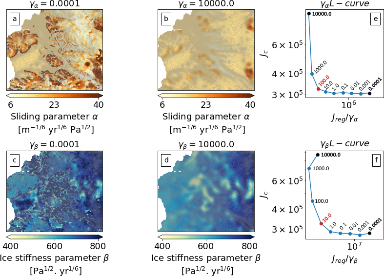
Figure 3L-curve analysis output. (a, b) Sliding parameter (α) computed using extreme γα values (bold values in panel e). (c, d) Ice stiffness parameter (β) computed using extreme γβ values (bold values in panel g). (e, g) L-curve analysis for γα and γβ. The optimal values suggested by the L curves are highlighted in red.
We generate L curves by varying the smoothing parameters γ and δ rather than the variance and length scale arising from a physical interpretation of the prior (Sect. 2.6). Both L curves in Fig. 3e and f are computed independently from each other – i.e. varying one parameter over several orders of magnitude while the other three parameters remain fixed (L-curve model configurations are shown in Table A1). To shorten this analysis we show only L curves for γ in Fig. 3; L curves for δ can be found in Appendix A2. The L curves presented in Fig. 3e and f are created by using ITS_LIVE surface velocities to find the misfit (Eq. 7) and by plotting the regularization terms against the cost function value Jc, as the regularization terms γα and γβ (Eq. 12) vary over several orders of magnitude (104 to 10−4).
In order to understand the effect that the strength of the regularization (or prior strength) has on the control parameters, we show α and β spatial distributions computed using the extreme values of the L curves (see Fig. 3a to d). If the prior strength is strong (i.e. a large γα) the inverted parameter field (in this case the sliding coefficient) is relatively smooth (see Fig. 3b) and Jc generally small. The L curve for γα in Fig. 3e suggests γα=100.0 as a reasonable trade-off between the cost function value and the regularization term. For γβ this value is 1 order of magnitude smaller (γβ=10.0, see Fig. 3f). For δα,β the L-curve analysis suggests a value of (see Table A1 for all parameter statistics and units). We used those values to conduct the rest of the experiments presented in Sect. 4.2 and 4.3.
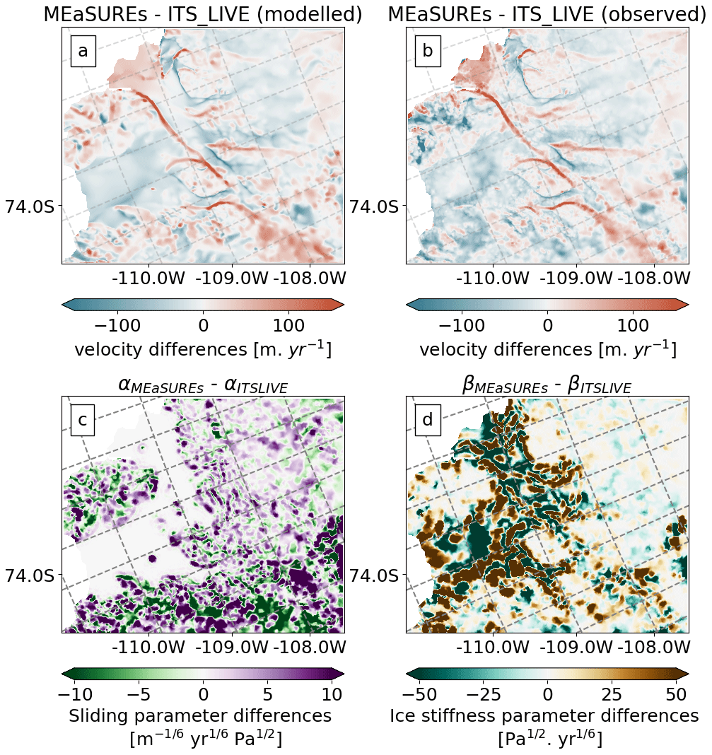
Figure 4Inversion output differences after using two different satellite velocity products (MEaSUREs and ITS_LIVE) to calibrate the ice dynamic parameters. (a) Modelled velocity differences (b) Observed velocity differences. (c) Sliding parameter (α) differences. (d) Ice stiffness parameter differences (β).
4.2 Model output computed with different ice velocity observations
We use the regularization parameters found in the previous section and run all stages of the error model framework (all methods in Sect. 2) twice using different satellite velocity products for each run: MEaSUREs and ITS_LIVE. We compare the observed ice velocity from both products in Fig. 4b and find significant differences (≥100 m yr−1), especially at the ice margins. The assimilated states of FEniCS_ice reproduce these differences as shown in Fig. 4a, where we show modelled velocity differences between the two runs. Consequently, the inverted parameters from both runs are also different (see Fig. 4c and d). Differences in the output from both inversions are particularly large at the ice margins, and in the case of the ice stiffness parameter β, the largest differences are found at the Crosson and Dotson ice shelves (see Fig. 4d). The projections of VAF differ as well: after 40 years, the difference in VAF is approximately 3.9×10¹¹ m3, or 390 km3 – nearly 15 % of overall VAF loss (Fig. 5a).
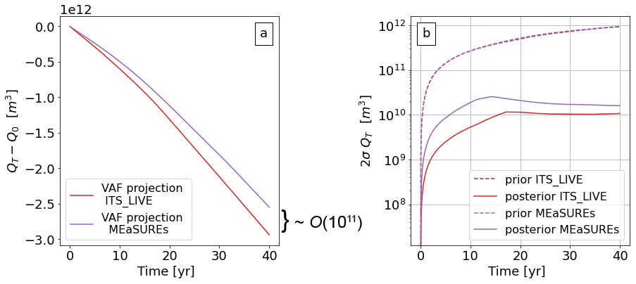
Figure 5(a) Trajectories of change in VAF (i.e. QT−Q0) using different velocity products and the regularization terms suggested by the L curves (γα=100, γβ=10). (b) Hessian-based prior (dash lines) and posterior (solid line) uncertainties of VAF over time (2σQT represents the 95 % confidence interval).
Figure 5b shows estimated posterior uncertainty of VAF loss after 40 years from our Hessian-based framework in our L-curve-informed workflows. The uncertainty estimates are on the order of 10 km3 (10 km3 for the ITS_LIVE-constrained inversion and 16 km3 for MEaSUREs) – an order of magnitude smaller than the observed difference. These results are seemingly at odds. In other words, our error propagation framework suggests a forecast uncertainty that is 1 order of magnitude smaller than the variability in VAF found when using two different satellite velocity products. This leads to a contradiction, as it suggests that our observed variability in VAF loss is extremely unlikely (see the Discussion section). This contradiction could arise from one or more of the following: (i) the regularization suggested by the L-curve analysis is too strong, i.e. the prior is overly informative; (ii) the observational error covariance matrix used for ITS_LIVE does not capture the true variability of the velocity field shown in Fig. 4b (see Sect. 3.1.3); and/or (iii) there are too many data points informing our cost function. We address point (iii) in the next section, whereas points (i) and (ii) are addressed in Sect. 5.2 and 5.1.
4.3 Effect of observational data subsampling
In this section we develop a metric to evaluate the quality of the model's inversions if we decrease the number of observations. In other words, we study the effect that different data densities have on the cost function performance. Similar techniques have been used to gather information on cross-correlations between two different sets of observations (e.g. covariance between winds speed observations in Desroziers et al., 2005). Here we apply a similar diagnostic test to study the covariance between adjacent velocity observations from the same product. Additionally, Koziol et al. (2021) show that data density affects the posterior covariance of the control parameters for an idealized experiment; thus, we use the results of this metric to test how data density affects the posterior uncertainty of VAF in Sect. 5.2. The test has the following steps.
-
Produce several training datasets of observed ice velocity by retaining different percentages of data points from a given set of observations (e.g. ITS_LIVE).
-
Use those training sets to compute inversions of α and β using our L-curve-informed prior configuration.
-
Use the α and β results from step 2 to evaluate (Eq. 8) on velocity points that were not used to compute the inversions (i.e. using a validation dataset with observations from a different product such as MEaSUREs).
Based on metadata from both products (see Sect. 3.1), we consider MEaSUREs and ITS_LIVE velocities to be two independent realizations of the state of the ice sheet at a given time and location. Hence, we use ITS_LIVE velocities for training and MEaSUREs for validation.
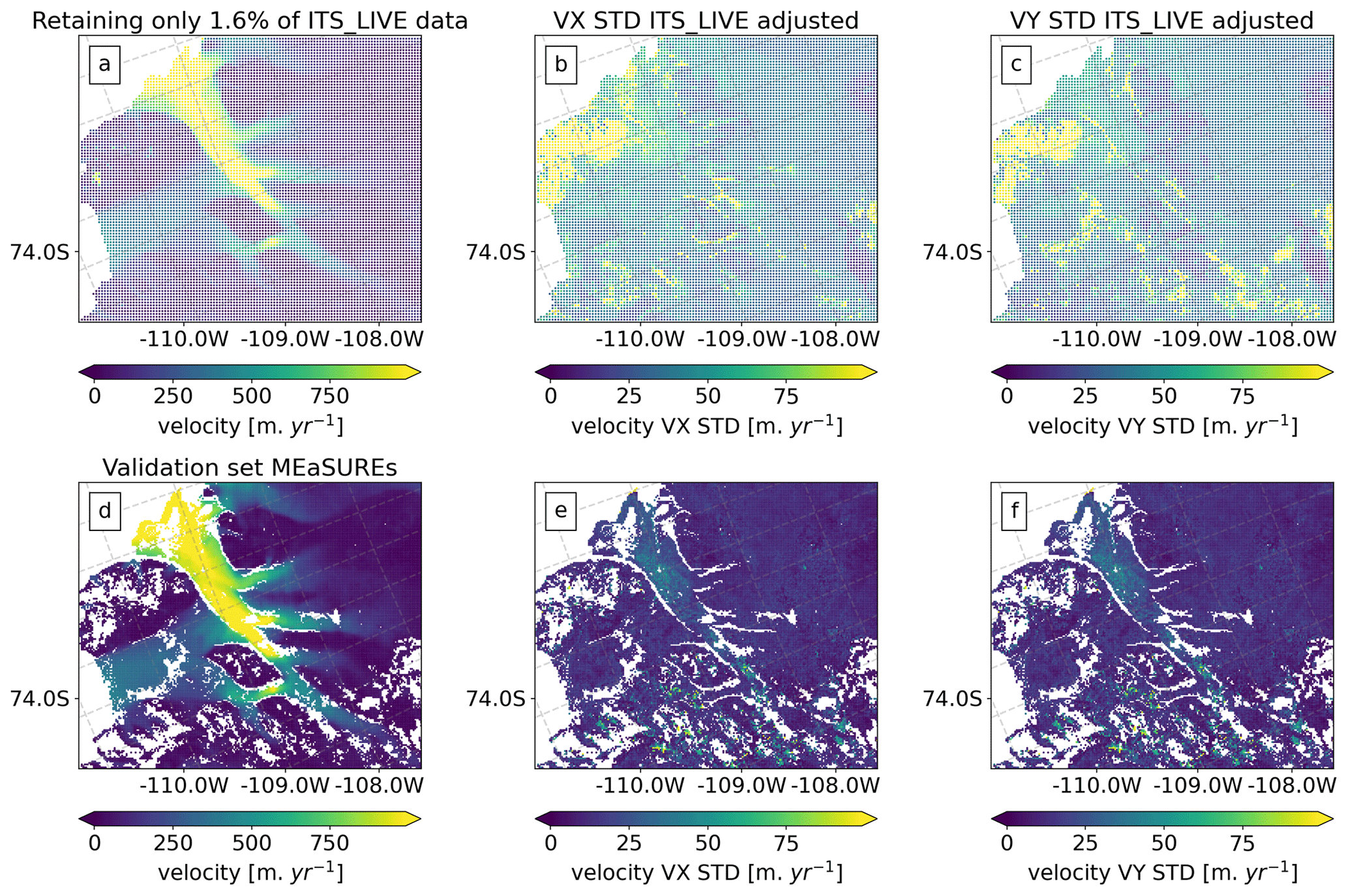
Figure 6Overview of the input data used for the observational data subsampling test and for the experiments presented in Sect. 5. (a) Example of a training dataset from ITS_LIVE where only 1.6 % of the data points are retained. (b, c) ITS_LIVE uncertainty in the x and y direction with the same data density as in (a) and with the SD of each component adjusted (see Sect. 5.2 for details). (d–f) MEaSUREs validation dataset used for the test.
To construct the training sets, we divide the domain into cells of different sizes (different grid-spacing) and systematically drop observations by iterating over the x and y directions of the ITS_LIVE grid. We select subsamples of the data by retaining corner and centre observations from each cell per iteration – i.e. upper and middle cell points. An example of a training dataset is shown in Fig. 6a, where we retain only 1.6 % of the velocity observations. To construct the validation set, we downscale MEaSUREs to the ITS_LIVE resolution and drop problematic data points (see Fig. 6d to f), i.e. locations where MEaSUREs and ITS_LIVE present velocity differences higher than 50 m yr−1 (as shown in Fig. 4b).
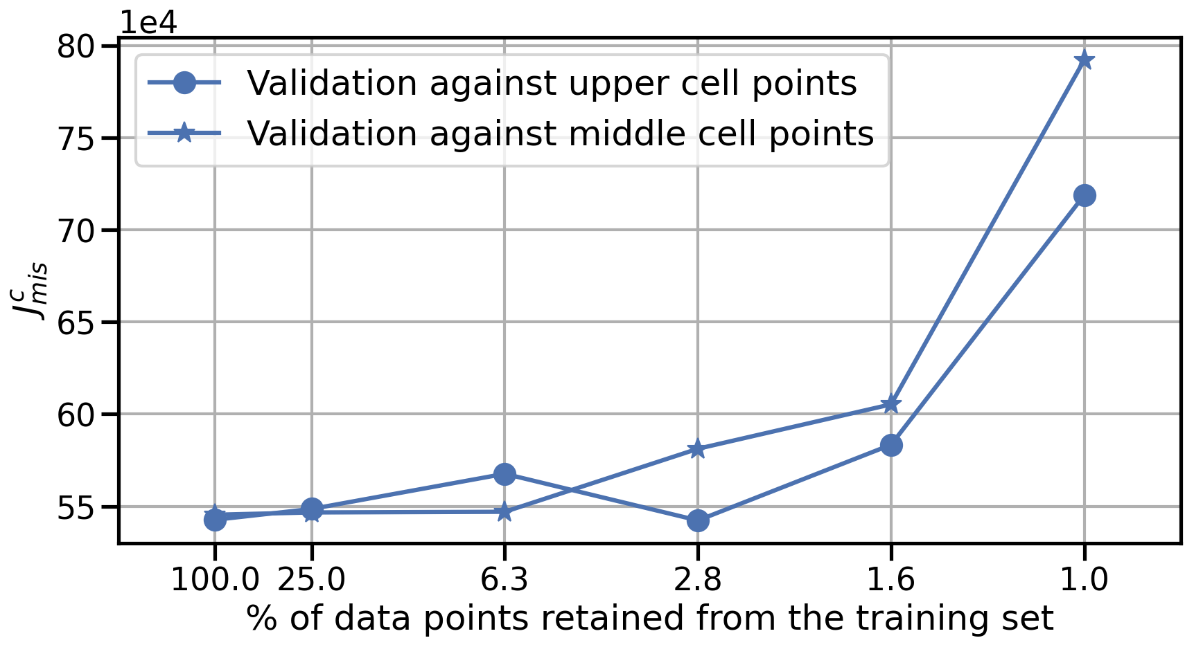
Figure 7Observational data subsampling results. performance if retaining a different number of observations for each training set.
Results of the test (see Fig. 7) demonstrate that our framework provides robust inversions for the drag and stiffness parameters α and β. Additionally, these results reveal that the value of does not change significantly even when we retain only 1.6 % of the data, which suggests that a large number of data points may be redundant when inverting for the control parameters, with potential implications for the error propagation of VAF (see the results from Sect. 5.2). However, observations are needed to inform the model in critical areas of the domain (i.e. at the grounding line or calving fronts), and if we drop observations in a random manner the performance of may decrease.
Results from Sect. 4.2 show that if we use the prior strength suggested by the L curves and the original ITS_LIVE velocity and standard deviation (SD), our framework underestimates the posterior uncertainty of VAF loss after 40 years by 1 order of magnitude (see Fig. 5b). More precisely, we calculate a posterior uncertainty which suggests that the difference in projected VAF (estimated by using two velocity products that nominally observe the same physical properties to calibrate our model) is extremely unlikely (see Fig. 5a). To achieve a posterior uncertainty that reflects the same order of magnitude, i.e. ∼ O(1011 m3), we carry out two more experiments aiming to understand how the uncertainty in the forecast of VAF is affected by the use of different strengths of prior (Sect. 5.1) and different versions of the ITS_LIVE data (Sect. 5.2). Additionally, we study the impact of using different sliding laws on the posterior uncertainty of VAF (Sect. 5.3).
5.1 Impact of using different prior strengths on the posterior uncertainty of VAF
We keep the same velocity input for all model configurations trialled in this section (i.e. retaining only 1.6 % of the ITS_LIVE data and adjusting the observations SD, as explained in Sect. 5.2) but vary the strengths of the prior. We experiment with the variance and auto-covariance length scale lc(0) of each control parameter instead of using priors suggested by L-curve analysis, as these definitions (see Sect. 2.6) have a more physical meaning. We calculate prior strengths using Eq. (18) and by making an informed guess for and lc(0) based on existing prior knowledge and physical concepts that define each control parameter.
From the literature (Pattyn, 2010; Khazendar et al., 2011; Still et al., 2022) we know that the spatial pattern of the ice stiffness is not uncorrelated. The advection of colder tributary glacier ice onto the ice shelf is well represented by the vast expanses of stiffer ice originating at the grounding line and extending downstream for tens of kilometres (see panels c and d of Fig. 3), whereas observed deformation patterns at the shear margins (Khazendar et al., 2011; Still et al., 2022) suggest the presence of weaker deformable ice, where the prominent formation of crevasses occurs. Thus, we keep an auto-covariance length scale lβ(0) for β equal to 1 km in all prior configurations, as crevasses can be present within that length scale. In future studies this length scale could be set by conducting a detailed spatial statistical analysis of crevasse maps derived from remote sensing, which is beyond the scope of this study. For we trial variance values computed from the SD of the ice stiffness (B) initial guess (see details in Sect. 3).
For the sliding parameter we define auto-covariance length scales lα(0) that are slightly larger than those assumed for β (i.e. 2 to 3 km), as observations from airborne radar over the ice sheet (De Rydt et al., 2013) verify that for fast-flowing ice streams, the surface topography carries important information about the bed with wavelengths between 1 and 20 times the mean ice thickness (≥ 1 km), thus controlling basal sliding at similar scales. Additionally, model experiments described in Gudmundsson (2008) show that the SSA overestimates the effects of bed slipperiness perturbations on the surface profile for wavelengths less than about 5 to 10 times the mean ice thicknesses, with the exact number depending on values of surface slope and slip ratio. Variance values are less intuitive; thus, we trial values over several orders of magnitude in order to vary the prior strength imposed on α.
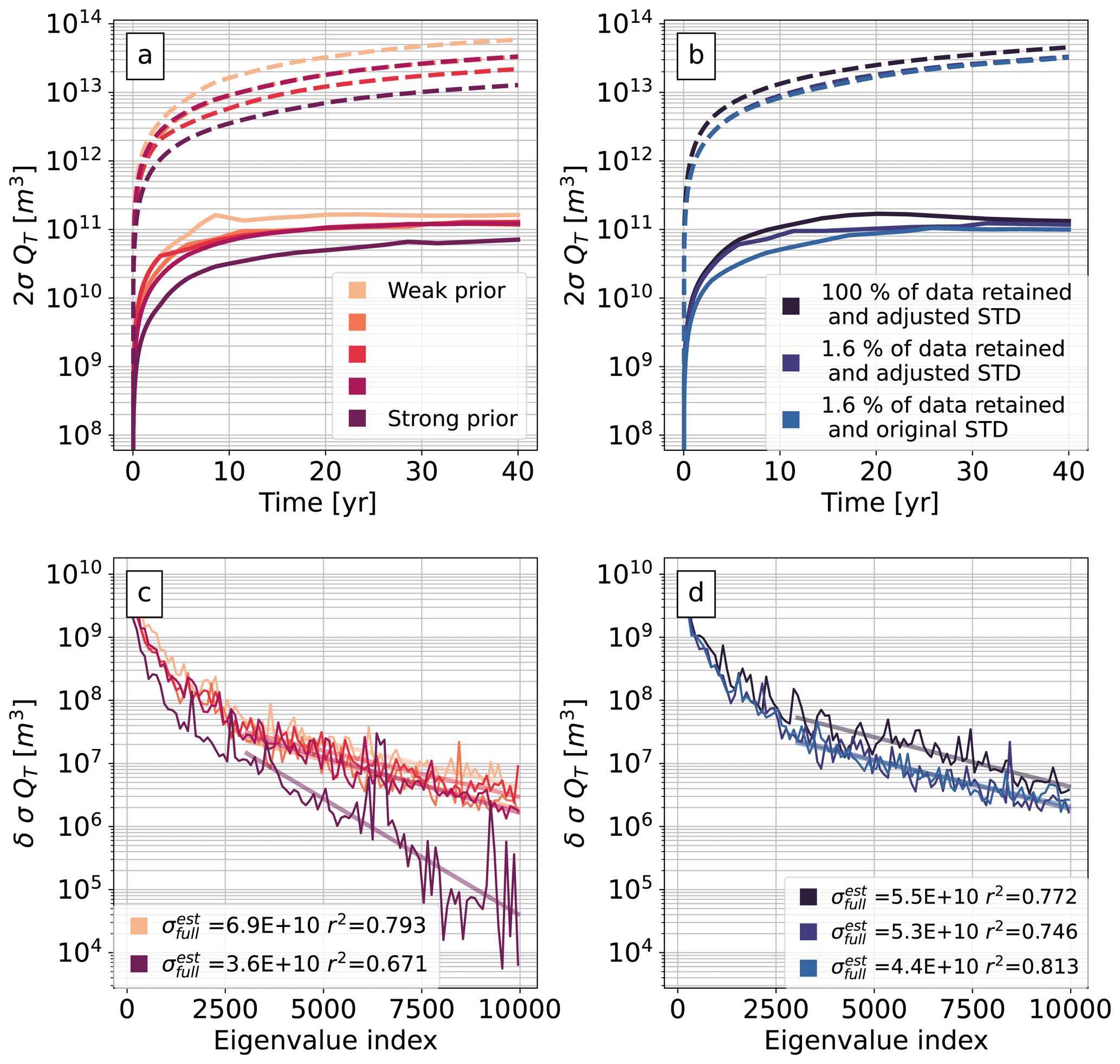
Figure 8Hessian-based prior (dash lines) and posterior (solid line) uncertainties of VAF over time (2σQT represents the 95 % confidence interval) computed using (a) different strengths of the prior and (b) different versions of the ITS_LIVE data (i.e. different data density and SD; see details in Sect. 5.2). (c, d) Rate of change for the posterior uncertainty of VAF (δσQT) against the number of eigenvalues calculated; statistics are shown in the lower corners, i.e. , the estimated SD of VAF for an infinite number of eigenvalues, and the decreasing trend coefficient of determination (r2).
Table 1Prior strength configurations used in Sect. 5.1 and 5.3, based on the pointwise standard deviation σc(0) and auto-covariance length scale lc(0) of each control parameter, ordered from weak to strong (except for the Cornford sliding law experiment).
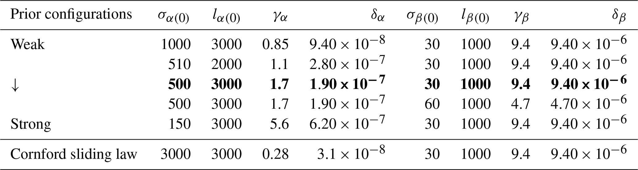
The configuration in bold is also used in the experiments of Sect. 5.2 and 5.3. The units of σα(0) are m yr Pa and σβ(0) are Pa yr. The unit of the auto-covariance length scale lc(0) is reported in metres (m). Following Eq. (18), the units of γα are m yr Pa, γβ are m Pa yr, δα are m yr Pa, and δα are m−1 Pa yr.
The resultant prior strengths are shown in Table 1, and the estimated posterior uncertainty of VAF for each prior configuration is shown in Fig. 8a (solid lines). Both are ordered from weak to strong. For the weakest prior we find an uncertainty of approximately 160 km3 – an order of magnitude larger than the estimates found previously. This suggests that a strong prior on the sliding parameter (such as the one suggested by the L-curve analysis) suppresses the error propagation from the satellite data onto projections of VAF. Most of our prior experiments focus on α; however, we also trial our error propagation framework changing the variance of β (see Table 1). Compared to prior experiments run on α, changing β priors show little influence in the posterior uncertainty of VAF. We also test weaker priors for both parameters, but these experiments lead to non-stable solutions of the time-dependent SSA as the parameters present undesirable and nonphysical features (not shown).
Our low-rank approximation to the Hessian (Eq. 16) makes the assumption that if additional eigenvectors were retained (i.e. if r were larger) the estimated posterior uncertainty σ(QT) would not change considerably. To test this we examine the marginal change in σ(QT) for each r (see Fig. 8c), which exhibits an approximately exponential decay with r. To estimate the effect of the low-rank approximation we assume that the decay rate holds up to r=N, where N is the full problem size, and that all neglected terms in Eq. (16) make a negative contribution to σ(QT) – i.e. we estimate the “worst case” in which every extra eigenvector and eigenvalue calculated decreases the uncertainty (see Appendix B for details of this estimate). The resulting estimated SDs of VAF for an infinite number of eigenvalues are shown in the captions of Fig. 8c and indicate that for all prior strengths, even in the worst case, posterior uncertainties decrease by a small proportion and more importantly are not as small as those values seen in our L-curve investigations. We perform this same check in all remaining experiments and observe similar results (see Fig. 8d and Fig. 10f).
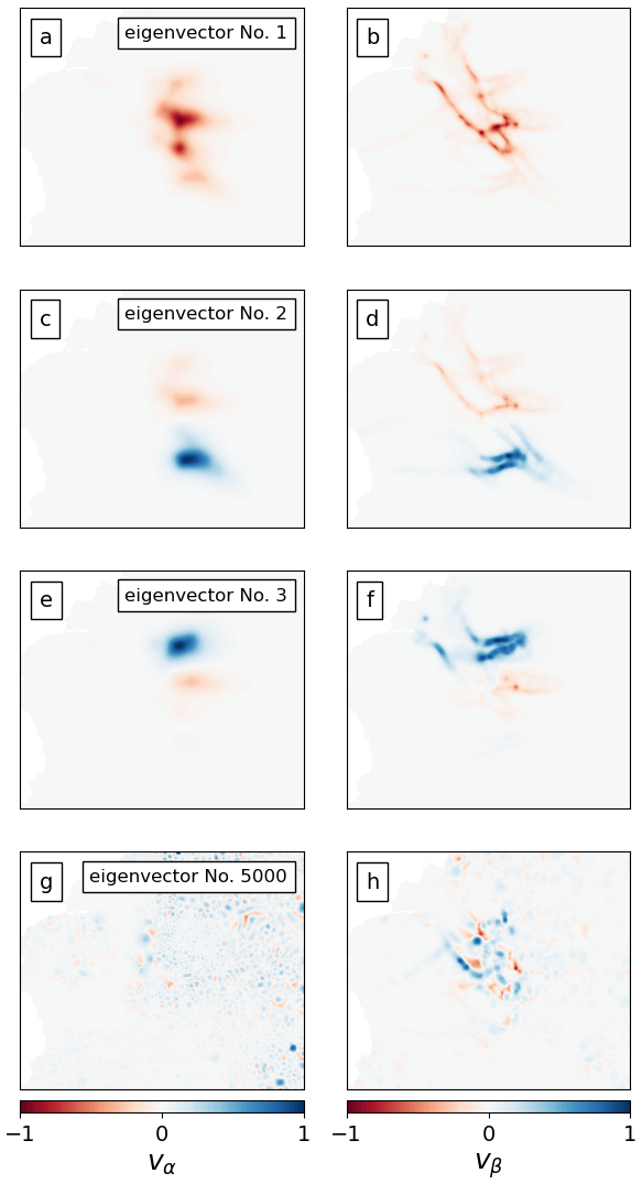
Figure 9Eigenvectors (v) of the Hessian. Each eigenvector has an α component (right column) and a β component (second column). Each component is scaled to have a maximum magnitude of 1. Ordered from large to small (from top to bottom), these v values correspond to the 1st, 2nd, 3rd, and 5000th eigenvalues.
Finally, the retained eigenvectors from the Hessian can be interpreted as modes in the parameter space that change the approximated posterior uncertainty relative to the prior uncertainty. We show in Fig. 9 the leading eigenvectors (see panels a to f) for the prior configuration highlighted in Table 1. The dominant eigenvectors of the ice stiffness parameter field β (panels b, d, and f) suggest that we gained more information regarding this parameter at the grounding line. The eigenvector corresponding to the smallest eigenvalue (Fig. 9h) is increasingly more oscillatory (and thus provides information at smaller length scales in the parameter space) and is increasingly relatively less informed by the velocity observations; such patterns are also present in similar studies (e.g. Isaac et al., 2015).
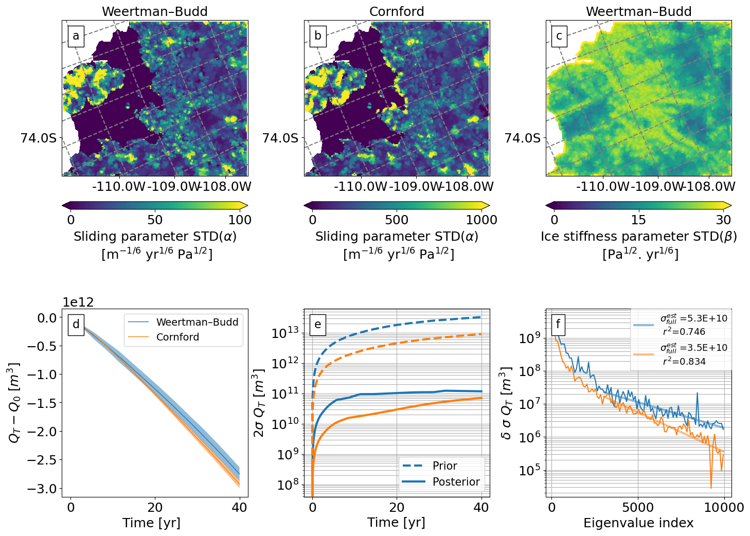
Figure 10Model output when using two different sliding laws. Pointwise SD of the sliding parameter α for the (a) Weertman–Budd and (b) Cornford law. (c) Pointwise SD of the ice stiffness parameter β (independent of the sliding law). (d) Trajectories of change in VAF (QT−Q0) using the different sliding laws and the highlighted weak prior from Table 1. (e) Hessian-based prior (dash lines) and posterior (solid lines) uncertainties of VAF over time (2σQT represents the 95 % confidence interval). (f) Rate of change for the posterior uncertainty of VAF (δσQT) against the number of eigenvalues calculated; statistics are shown in the lower corners, i.e. , the estimated SD of VAF for an infinite number of eigenvalues, and the decreasing trend coefficient of determination (r2).
5.2 Impact of using different ice velocity observations on the posterior uncertainty of VAF
Contrary to the previous section, here we keep the same prior strength for all the experiments but modify the velocity input. We modify the original ITS_LIVE data by decreasing the number of observations and by adjusting the SD of each velocity component to match the following condition:
where vxsd and vysd are standard deviations of velocity components, and the I and M subscripts refer to ITS_LIVE and MEaSUREs, respectively. In other words, where the original uncertainty of the data is small, we replace the SD of those coordinates with the absolute difference between MEaSUREs and ITS_LIVE velocities at that same location. Figure 6b and c show this error adjustment for each velocity component. We generate three versions of the ITS_LIVE data by (i) retaining all data points but adjusting the SD, (ii) retaining only 1.6 % of the data (in line with the results from the observational data subsampling test) and adjusting the SD, and (iii) retaining only 1.6 % of the data but keeping the original SD.
We run our error propagation framework using these three datasets (and the weak prior configuration highlighted in Table 1) and compute VAF posterior uncertainties as shown in Fig. 8b (see solid lines); uncertainties in this figure are plotted from high to low (from dark to light blue) and represent a 95 % confidence interval. The effect of retaining only 1.6 % of the observational data leads to a slight decrease in posterior VAF uncertainty – which is counter-intuitive as one would expect fewer observations to give a larger posterior calibration uncertainty. However, the VAF uncertainty (Eq. 15) is derived from both calibration uncertainty and VAF sensitivity. The latter differs between the experiments, as can be seen from the projection of prior uncertainty onto VAF sensitivity (blue dashed lines). The adjustment of observational SD increases VAF uncertainty at approximately 5 to 15 years but has less impact after. Importantly, however, the overall impact on the posterior uncertainty of VAF loss after 40 years is small relative to the effect of changing the prior strength (see solid line differences between panels a and b of Fig. 8).
5.3 Impact of using different sliding laws on the posterior uncertainty of VAF
In previous configurations we use the Weertman–Budd sliding law, but due to the sensitivity of the time-dependent ice sheet model to the choice of sliding law (Brondex et al., 2019; Kazmierczak et al., 2022; Barnes and Gudmundsson, 2022) we trial our error propagation framework using the Cornford law and compare qualitative differences from both laws in Fig. 10. We use the same velocity constraints (i.e. the same as in Sect. 5.2) and consider only a single prior distribution. Ideally, we would need to investigate a range of priors for the Cornford law (as we did for Weertman–Budd in Sect. 5.1), but this is beyond the scope of our study. The prior distribution used is similar to the highlighted parameters in Table 1, but with a modified – since in the interior the basal stress is independent of the effective stress (Cornford et al., 2020), and thus we expect variations of α to have a different scale (see last configuration in Table 1).
Using the inverse of the low-rank update approximation for the cost function Hessian (Γpost) we can estimate the posterior standard deviation (SD) of α and β. We divide the mesh into “patches” of approximately 1 km in diameter, and for each patch we compute the mean of each control parameter. We treat this mean as a new quantity of interest (QoI) and compute its SD via the same framework as projections of VAF loss (see Sect. 2.5). Essentially, in panels (a) to (c) of Fig. 10 we visualize the posterior of a “local average” of α and β.
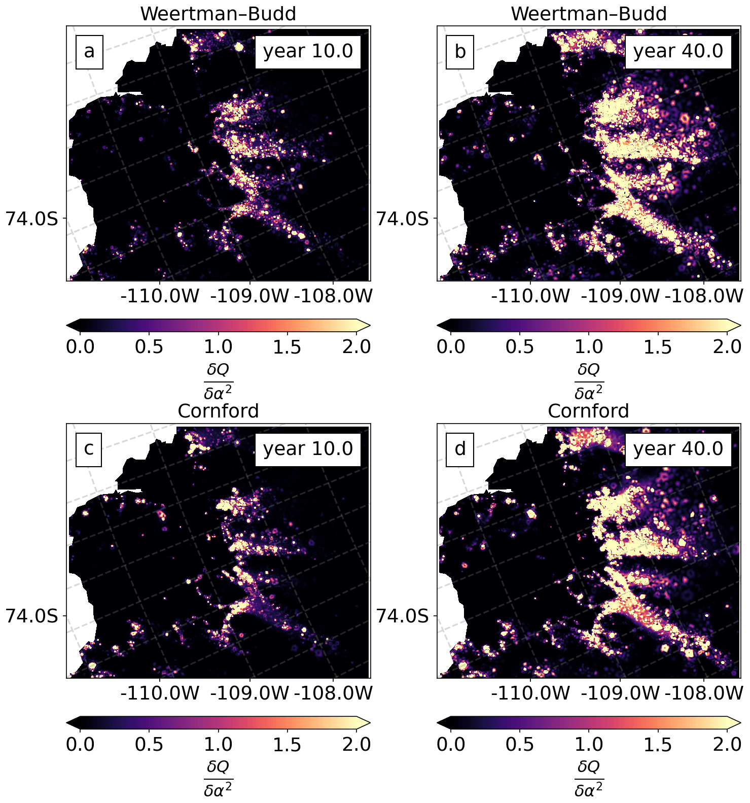
Figure 11Sensitivity maps of the model's change in volume above flotation (QT) to the basal friction coefficient α2 for year 10 and year 40 when using two different sliding laws. Units of α2 are m yr Pa. (a, b) Weertman–Budd and (c, d) Cornford law. These visualize the node-wise sensitivity given the choice of mesh and finite-element discretization.
For both sliding laws the sliding parameter α is more uncertain close to the grounding line and at the Bear Peninsula (see Fig. 10a and b) where uncertainties from the ITS_LIVE product are higher (see Fig. 2b and c). The large uncertainty just at the grounding line in the Cornford results (relative to that of Weertman–Budd) is due to the insensitivity of basal stress to α when the ice is near flotation (see sensitivity analysis below). For the ice stiffness parameter β the most uncertain areas of our domain are the grounding lines of the PSK glaciers and the Crosson ice shelf (see panel c of Fig. 10) – these are the areas where the speeds from the two satellite products show significant differences (see Fig. 4b).
For both sliding laws, VAF uncertainty reaches a similar order of magnitude ∼O(1011) m3 at year 40 (Fig. 10e). However, a quantitative comparison is somewhat misleading, as the impact of prior strength is not investigated for the Cornford law. There are qualitative differences, however: the posterior uncertainty of VAF for each sliding law saturates at a different rate, with the posterior uncertainty of the Cornford law configuration growing at a faster rate after year 10. We compare sensitivity maps of the model's VAF estimates to the basal friction coefficient α2 at years 10 and 40, normalized to year 40 sensitivities for the respective experiment (see Fig. 11). VAF sensitivities at year 10 computed using the Weertman–Budd law have a higher sensitivity to the basal friction coefficient relative to those computed using the Cornford law – particularly at the grounding line of Kohler Glacier (see panels a and c of Fig. 11). Additionally, Fig. 11 shows that at year 40 both sliding laws have similar sensitivities. In this section we only show sensitivity maps for α2; sensitivities to the ice stiffness are shown in Fig. A3 of Appendix A.
The efficiency of our error propagation framework allows us to explore how different prior strengths, velocity inputs, and sliding laws affect the uncertainty of VAF projections. We find that by choosing different satellite ice velocity products (that nominally observed the same physical properties to calibrate FEniCS_ice) our model leads to different estimates of VAF loss after 40 years (see Sect. 4.2). This effect may be less important for ice streams strongly coupled to ocean forcing (Lilien et al., 2019; Goldberg and Holland, 2022) but could be more influential for unstable margins (Joughin et al., 2014).
The differences in VAF trajectories (shown in Fig. 5a) computed using the different velocity products allow us to additionally identify issues in our initial prior probability densities computed using the L-curve criteria. The observed differences are extremely unlikely to be seen under the posterior densities informed by L-curve analysis, whereas they are far more likely under the posterior informed by physically motivated priors. The regularization suggested by the L curves is thus too strong and thus suppresses the error propagation from the satellite data into the QoI, resulting in VAF projections with quantified uncertainties that are too low.
Our analysis also suggests that the error provided with the velocity products cannot fully explain the variability in ice velocities observed in Fig. 4b and that large numbers of data points may be redundant, with implications for the error propagation of the QoI.
Our ice sheet flow model described in Sect. 2 can be thought of as a (nonlinear) mapping from a set of input fields, which might be unobservable or poorly known (α and β fields), to a set of output fields, which might correspond to observable quantities (e.g. satellite surface velocity observations). In FEniCS_ice, the parameter-to-observable map is a composition of two functions: the solution of the SSA equations (see Sect. 3 of Koziol et al., 2021, for details) and the misfit term (Eq. 8).
Our error propagation framework considers the ice sheet inverse problem as a linearized inverse problem; by linearization we mean that is linearized about the MAP point. Thus, the framework relies on a number of key assumptions related to this and other issues.
-
(i) The observational errors and prior distributions are defined as Gaussian distributions, (ii) the parameter-to-observable map is linear (or close to linear), and (iii) the quantity of interest (i.e. VAF) at a given time depends linearly (or nearly linearly) on the control parameters – in other words, the parameter-to-QoI map is close to linear.
-
The difference between velocities predicted by the model and the observations is due only to measurement errors (we assume zero model error; see Sect. 2.4 – or more precisely we consider conditional posterior information given the model).
-
The observational error covariance matrix is diagonal; i.e. errors in observations do not correlate spatially.
-
The posterior covariance of the control parameters Γpost is fully sampled with the number of eigenvectors and eigenvalues that we retain from the Hessian.
Note (1i, ii) that the above implies a Gaussian posterior. We test point (4) in Sect. 5.1 and address points (1)–(3) in the following subsections.
6.1 Linear dependence of parameter-to-observable and quantity of interest maps with respect to the control parameters
FEniCS_ice computes a second-order approximation to the posterior covariance of the control parameters Γpost (via the eigendecomposition of the cost function Hessian evaluated at the MAP point; see Sect. 2.5) and propagates forward the associated calibration uncertainty in time-dependent estimates of VAF loss (our QoI). The posterior PDF of is not guaranteed to be Gaussian due to the nonlinearity of the Stokes equations that describe . Furthermore, the propagation step (Eq. 15) is based on a linear transformation of a Gaussian random variable and assumes that , the parameter-to-QoI map, is well described by linear sensitivities.
Petra et al. (2014) test the Gaussianity of the parameter-to-observable map by sampling from the posterior PDF of the hidden field via different Markov chain Monte Carlo (MCMC) sampling methods (Tierney, 1994), including a new stochastic Newton method with a MAP-based Hessian. They solve a two-dimensional flow-line ice sheet inverse problem with a moderate number of parameters (∼100). It is suggested that for control parameter directions which are more strongly informed by observations, and in the weak observational noise limit, the posterior may be closer to Gaussian due to the weaker influence of the nonlinearity of . It is further suggested that for directions which are weakly informed by observations, and hence for which the Gaussian prior dominates, the posterior may again be closer to Gaussian. Therefore, a Hessian-based approximation (such as the one describe in Sect. 2.5) to the posterior covariance of the parameters may be useful despite the nonlinearity of .
Koziol et al. (2021) test the linearity of the FEniCS_ice parameter-to-QoI map for an idealized ice sheet flow problem (Pattyn et al., 2008) through a simple Monte Carlo sampling of the posterior PDF of . The study finds strong agreement with the linearly propagated posterior covariance when there is a moderately strong prior, but slightly poorer agreement with a weak prior.
Unfortunately, due to the size of our parameter space, testing the Gaussianity of the posterior PDF of is beyond the scope of our study. Similarly, sampling the posterior PDF to validate the propagation of calibration uncertainty to the QoI as in Koziol et al. (2021) would be intractable for our more realistic setting. Instead, we develop a simple test to check the linearity of the parameter-to-QoI map and how this linearity is affected when we impose different strengths of the prior. We test the linearity of the parameter-to-QoI mapping by using data from Sect. 4.2 to compute the following dot products:
Here I and M indicate model output computed by using either ITS_LIVE or MEaSUREs velocities. We visualize the linearity of the VAF operator by plotting each dot product together with the absolute difference between VAF trajectories computed using ITS_LIVE and MEaSUREs. Additionally, we repeat this test for a stronger prior configuration by imposing a strong regularization on β (stronger than the one suggested by the L-curve analysis, γβ=100.0).
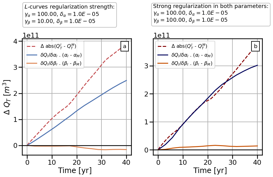
Figure 12Linearity test results. Absolute difference of trajectories of VAF (QT) estimated using different satellite velocity product (red dotted lines) and dot product results (solid lines) from Eqs. (23) and (24) plotted in blue and yellow, respectively. For this figure we use model output from Sect. 4.2. (a) Linearity test using the regularization strength suggested by the L curves and (b) linearity test using a stronger regularization on β.
Results from both tests are shown in Fig. 12 and verify that VAF estimates over time are highly dependent on α and that the linearity of the parameter-to-QoI map depends on the strength of the regularization (as in Fig. 12b and in Koziol et al., 2021). The main objective of this study is to propagate calibration uncertainty into projections of VAF loss. We find that in order to do so, we must impose a weaker prior on the control parameters than widely used methods (i.e. L-curve analysis) would suggest. But as shown above, in doing so we might need to compromise on the linearity of the parameter-to-QoI map. Moreover, as shown in Koziol et al. (2021), a weaker prior means a weaker spectral decay of the prior-preconditioned Hessian spectrum, requiring us to retain more of its eigenvectors (see also Sect. 5.1).
In other words, to avoid the prior probability from overwhelming the likelihood in our Bayesian inversion, we are required to examine a regime where we compromise the linearity of the time-dependent model in certain areas of the domain. Still, we expect that the framework can provide an “order-of-magnitude” estimate of the contribution of calibration uncertainty to QoI uncertainty. Although not previously applied to a problem as large as the present study, stochastic Newton MCMC (Martin et al., 2012; Petra et al., 2014), which does not rely on a Gaussian assumption, may provide a more robust estimate in such regimes. Importantly, to be tractable this method requires a reasonable estimate of the posterior density (the “proposal density”) – and such an estimate can be provided using the low-rank Hessian approximation generated within our framework. Thus, stochastic Newton MCMC may be a viable approach for non-Gaussian uncertainty quantification in future studies.
6.2 Qualitative inspection of the model's structural and forcing uncertainty
We only quantify calibration (parametric) uncertainty in projections of marine ice sheet loss. We do not quantify structural or model uncertainty, i.e. errors that arise from the discretization of the inverse problem (Barnes et al., 2021) or from the formulation of the model and its ability to represent the physics of the system (Hill et al., 2021). In Sect. 5.3 we trial our error propagation framework with different sliding laws and examine the implications for projections of VAF loss (see Fig. 10), though quantifying the likelihood of various sliding law formulations is beyond the scope of our study.
In this section we look at uncertainty due to the use of different physics and discretization to solve the ice sheet momentum balance. We do this by using a second ice sheet model: the STREAMICE module of MITgcm (Goldberg and Heimbach, 2013), which solves a depth-integrated balance that accounts for vertical shearing (absent from the shallow ice stream approximation; Goldberg, 2011). STREAMICE solves the momentum balance on a regular rectangular grid, a distinct discretization from FEniCS_ice. With a uniform 500 m grid, we simulate with STREAMICE an instantaneous velocity field (without time evolution) using the inverted parameter fields of FEniCS_ice (interpolated to the STREAMICE grid) and the same geometry and boundary conditions described in Sect. 3. The particular fields of α and β are from our L-curve analysis (Sect. 4.1). We compare both models' surface velocities and find differences on the order of 100–200 myr−1, particularly in the fastest-flowing ice areas and on the ice shelves (see Fig. A4). FEniCS_ice and STREAMICE have different approximations to Stokes flow, employ different treatments of the grounding line in their equations, and have very different resolution, which may lead to this disagreement. Barnes et al. (2021) find similar results, when two other adaptive mesh, finite-element SSA models are compared to STREAMICE through the same diagnostic experiment. The authors show that these diagnostic calculations are not indicative of the performance of the models in time-dependent simulations (see Fig. 6 of Barnes et al., 2021, where all models reach similar projections of VAF).
We emphasize that this comparison cannot quantify structural uncertainty, but can inform us (qualitatively) of the effects of implementing different discretizations and grounding line formulations in the model numerics.
6.3 Relevance of calibration uncertainty versus structural and forcing uncertainty
As previously mentioned, structural uncertainty is neglected in our study and we use a very simple ocean forcing parameterization, for which uncertainties are not considered. We make it clear that our aim is to quantify calibration uncertainty alone; however, it is only worth doing so if the contribution of calibration uncertainty to forecast uncertainty is non-negligible and/or the framework represents nontrivial steps toward incorporating these other sources of uncertainty. Regarding the former, the existing literature provides some clues as to whether calibration uncertainty is important. Goldberg and Holland (2022) carry out coupled ice sheet–ocean modelling experiments for the PSK glacier region and show that the type of calibration of ice model parameters (i.e. whether fit to observed thinning is accounted for) strongly determines ice loss over 20–30 years; beyond this point, ice loss depends on far-field ocean conditions. For other catchments, this “crossover time” could be shorter or longer – meaning that uncertainty in calibration could inform projection uncertainty on the multidecadal scale before it is overtaken by climate uncertainty. The short-term persistence of calibration errors is echoed in other types of cryospheric modelling: Aschwanden and Brinkerhoff (2022) showed that the introduction of satellite-based information strongly reduced uncertainty in short-term projections of Greenland ice loss but that this relative information gain was greatly reduced by 2100, particularly under strong climate forcing scenarios. Still, calibration uncertainties should not be dismissed even if they are overwhelmed by climate forcing on long timescales: there are strong reasons why short-term (multidecadal) projections of ice loss are key for planning and mitigation (Bassis, 2022).
Moreover, our framework of estimating calibration uncertainty can easily be expanded to account for forcing uncertainty. Provided that forcing uncertainty is independent of parameter uncertainty, the contribution of forcing to projection uncertainty is additive and can be found using an expression similar to Eq. (15). Importantly, such a calculation is independent from the estimation of posterior parameter uncertainty through eigendecomposition of the Hessian – which is by far the most costly component. This is not true of model uncertainty: our likelihood PDF gives the probability of observable velocity conditioned on parameters and the model and hence neglects model uncertainty. A potential way to incorporate model uncertainty – once it is quantified – is to adjust the observational error covariance used in the likelihood. A similar approach has been used in the Bayesian error approximation method of Babaniyi et al. (2021).
6.4 Accuracy of observational error model
We draw the tentative conclusion that, for our study area, the choice of prior distribution informed by L-curve analysis is overly informative and underestimates calibration uncertainty. This is based on the fact that, with such a prior, the posterior VAF is an order of magnitude smaller than the variability in VAF between two widely used velocity products as constraining data. Essentially, the two products are treated as a two-member sample from a distribution describing the true surface velocities. While this is a very small sample size, our assessment makes the assumptions that (i) the posterior VAF distribution is Gaussian (which is explored above) and (ii) the two members are likely sampling outcomes under our observational error model – and therefore that the variation of ∼ O(1011 m3) is not a statistical outlier – thus, our Hessian-based assessment must be too small.
A further assumption in our assessment is that our observational error model is accurate. As described in Sect. 3.1.3, we use reported errors and standard deviations to define diagonal terms in Γobs and assume zero spatial error covariance. Error magnitudes may be underestimated – although we somewhat account for this by adjusting observational errors based on differences between the products (Sect. 5.2). Additionally, not accounting for spatial error correlation could underestimate calibration uncertainty, as shown in the idealized experiments of Koziol et al. (2021). It is possible that improved assessments of spatial observational error covariance may be needed to accurately quantify calibration uncertainty when calibrating ice sheet models with satellite-based data. Such approaches have been used in weather data assimilation (Tabeart et al., 2020).
This study set out to apply the FEniCS_ice error propagation framework to a realistic setting in West Antarctica (which includes three ice streams: Pope, Smith, and Kohler glaciers) and infer from satellite velocity observations two important unknown parameters in ice dynamics and its uncertainties: the basal sliding friction coefficient (α) and the rheological parameter for describing ice stiffness (β). As in many other ice sheet modelling studies we use a control method to calibrate grid-scale flow parameters. However, our framework augments the control method with a Hessian-based Bayesian inference approach, which characterizes the posterior covariance of the inverted parameters. We project calibration uncertainty forward in time and onto projections of volume above flotation (VAF).
We find that by choosing different satellite ice velocity products (that nominally observed the same physical properties to calibrate FEniCS_ice) our model leads to different estimates of VAF after 40 years or to different projections of sea level rise contribution. We use this difference in model output as an order-of-magnitude estimate of the variance that projections of VAF should have after 40 years and identify prior strengths that can reproduce that variability. We demonstrate that if we use prior strengths suggested by L curves, as is typically done in ice sheet calibration studies, our uncertainty quantification is not able to reproduce that same variability. The regularization suggested by the L curves is too strong (i.e. the information contained in the prior distribution computed via L-curve analysis dominates over the information contained in ice velocity observations) and thus suppresses the error propagation from the satellite data into VAF projections with quantified uncertainties that are smaller than those suggested by our two-member “sample” of observed velocity fields. Therefore, we recommend using the variance and length scale arising from a physical interpretation of the prior to define regularization parameters, as these definitions (see Sect. 2.6) will inform the ice sheet model with a more realistic spatial variability regarding the basal sliding and ice stiffness parameters.
Additionally, our experiments suggest that large numbers of data points may be redundant, with implications for the error propagation of VAF.
We qualitatively inspect one aspect of structural uncertainty by trialling our error propagation framework with two different sliding laws (Weertman–Budd and Cornford laws). The posterior uncertainty of VAF evolves differently for the two parameterizations, with the Weertman–Budd uncertainty saturating relatively quickly while that of Cornford steadily increases. This may be due to differing patterns of sensitivity of VAF to the sliding parameters, particularly near the grounding line.
Finally, our framework alone does not fully quantify sea level rise forecast uncertainty, but represents an important step. Further improvements to our method could be to (i) quantify calibration uncertainty through stochastic Newton Markov chain Monte Carlo (MCMC) using our Hessian eigendecomposition as the proposal density, (ii) take into account model error in the likelihood probability density function, and (iii) take into account forcing uncertainty in the error propagation framework.
A1 ITS_LIVE 6-month offset speed change
To study the 6-month offset between ITS_LIVE and MEaSUREs velocities, i.e. from July 2014 to December 2014, we subtract data acquired in 2014 from the 2018 ITS_LIVE velocity mosaic and divide this by 8 in order get the monthly changes (see Fig. A1a). The effect of the 6-month offset between the two products is negligible compared to the difference observed in Fig. 4b and to the speed ratio shown in Fig. A1b. However, there are significant differences (over a small area) at the calving front of the Crosson ice shelf (see Fig. A1a).
A2 δα L curve
In addition to the experiments shown in Sect. 4.1, we constructed an L curve only for δα and use the same result for δβ. Results are shown in Fig. A2 and suggest a value for δα of compared to values in Table 1. Any will result in a stronger prior, and thus we choose for the error propagation experiments shown in Fig. 3e and f.
A3 Sensitivity of VAF to the ice stiffness (B)
We compare sensitivity maps of the model's VAF estimates to the ice stiffness B (or β2) at years 10 and 40 (see Fig. A3). VAF projections are more sensitive to the ice stiffness at the grounding line of the PSK glaciers and at the Crosson ice shelf. In future studies, these sensitivity maps and the ice stiffness spatial distribution could be correlated with detailed spatial maps of crevasses in the area.
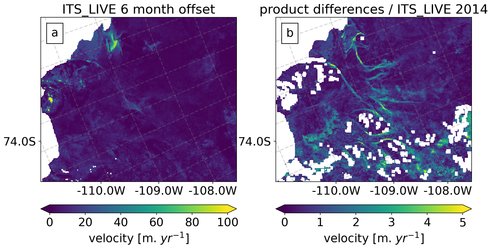
Figure A1Speed comparisons. (a) The 6-month offset speed change from ITS_LIVE 2014 (July–December) and (b) the speed ratio of the difference between the two products (ITS_LIVE 2014 – MEaSUREs acquired from July 2013 to July 2014) and ITS_LIVE 2014. Empty pixels in panel (b) are due to gaps in the MEaSUREs dataset, which increase when the data are interpolated to the ITS_LIVE grid.
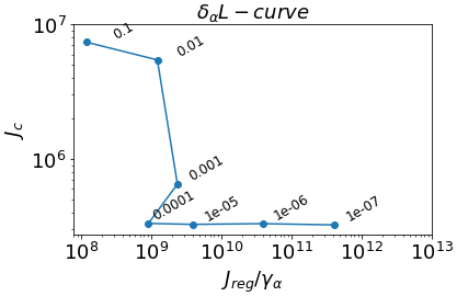
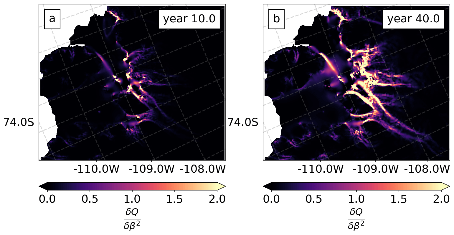
Figure A3Sensitivity maps of the model's change in volume above flotation (QT) to the ice stiffness (B or β2). Units of B are Pa yr.
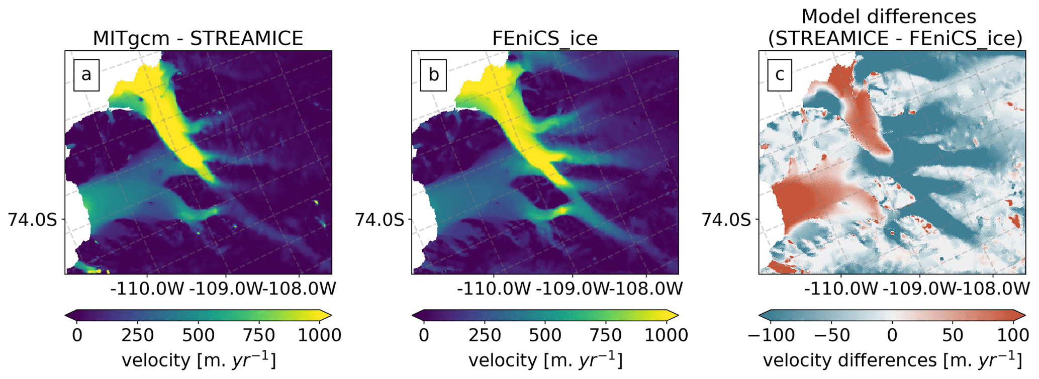
Figure A4The models' surface velocity comparison. Surface velocities are calculated by using FEniCS_ice inversions of α and β calibrated with ITS_LIVE and the highlighted weak prior configuration from Table 1. (a) STREAMICE. (b) FEniCS_ice. (c) Difference between the two models.
Table A1L-curve configurations used in Sect. 4.1. Reference values for β parameters are obtained from variance values computed from the SD of the ice stiffness (B) initial guess (see details in Sect. 3). Reference values for α parameters (first guess) are chosen heuristically and looking to maintain the linearity of the VAF operator and stable solutions of the time-dependent SSA.
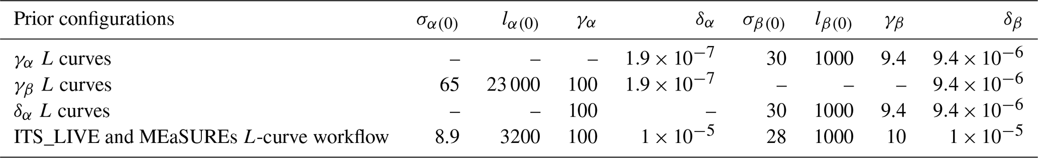
The dash (–) indicates that those parameters were varied by several orders of magnitude while constructing the L curves. The units of σα(0) are m yr Pa and σβ(0) are Pa yr. The unit of the auto-covariance length scale lc(0) is reported in metres (m). Following Eq. (18), the units of γα are m yr Pa, γβ are m Pa yr, δα are m yr Pa, and δα are m−1 Pa yr.
For each successive eigenvalue–eigenvector pair (λr, Cr) we construct the low-rank approximation to the posterior covariance using Eq. (16) and find the associated approximation to σ(QT) by projecting the estimated covariance onto the QoI (Eq. 15). We refer to this iteration here as σr – the posterior QoI uncertainty using the leading r eigenvectors – and to the difference as Δσr.
We observe that, for sufficiently large r, the absolute change with r can be represented reasonably well by an exponential decay, i.e.
for some b smaller than 1 (Fig. 8c and d). Assuming this to hold as r becomes large, we can estimate a lower bound for σ(QT)=σN (where N is the parameter dimension) with a geometric sum. Specifically, we find the d0 and b that best fit for , where rth is inferred from the decay of and rN is the number of eigenpairs retained (in our case 104). The relationship given by Eq. (B1) then implies for M>N
In Sect. 5 we use this result (with rth=3000) to estimate a lower bound for the posterior uncertainty of QT without low-rank approximation. The calculation is done at the final time, i.e. for T=40 only. We emphasize that this calculation is purely heuristic, and we are unaware of a theoretical lower bound for σM. Due to the tendency of the shallow-shelf approximation to filter high spatial frequencies in basal parameters (Gudmundsson, 2008), it is unlikely that will decay more slowly than predicted by Eq. (B1), and it may even decay more quickly. However, due to the large size of the parameter space (105) it is not tractable to find the full spectrum, so the estimate is not testable for this problem.
Finally, other studies use eigenvalue magnitude as a criterion for truncating the spectrum (e.g. Isaac et al., 2015). More specifically, eigenvectors are retained up to an index r such that . We note that this constraint alone does not ensure that the contribution to QoI uncertainty arising from the truncated part of the spectrum is negligible, even if the marginal contribution associated with each individual eigenpair is small.
The version of tlm_adjoint used in this paper is available in a permanent DOI repository (https://doi.org/10.5281/zenodo.7625841; Maddison and Recinos, 2023). The FEniCS_ice software, together with the application of the code to a real domain, is coded in the Python language and licensed under the GPL-3.0 license. The latest version of the FEniCS_ice code is available on GitHub (https://github.com/EdiGlacUQ/fenics_ice, last access: 4 October 2023) and Zenodo (https://doi.org/10.5281/zenodo.7615309; Maddison et al., 2023), and the documentation website of the model is under construction, but a user guide is provided (https://github.com/EdiGlacUQ/fenics_ice/blob/58742fc8c5dcda88ace9860a7c79cabb3160c374/user_guide/user_guide.pdf, last access: 2 October 2023). The code used to generate all figures and analyses of this study is available in a permanent DOI repository (https://doi.org/10.5281/zenodo.7615259; Recinos et al., 2023) and on GitHub (https://github.com/bearecinos/smith_glacier, last access: 2 October 2023) as is the FEniCS_ice version used for this study (https://doi.org/10.5281/zenodo.7615309; Maddison et al., 2023). We have constructed a documentation website for the application of the model to the domain of the PSK glaciers (https://doi.org/10.5281/zenodo.7615259; Recinos et al., 2023) where we explain in detail the installation of the code, the preparation of input data, and how to run and visualize the experiments presented in this study.
The output data of the model are available in the following permanent DOI repository: https://doi.org/10.5281/zenodo.7612243 (Recinos, 2023). Information about how to read and plot the data can be found in the Smith repository wiki – see https://github.com/bearecinos/smith_glacier/wiki (last access: 2 October 2023).
BR, DG, and JRM jointly conceived the study and contributed equally to the writing and development of the experiments presented in this paper. DG and JRM developed the mathematical framework implemented in FEniCS_ice. BR developed the Smith Glacier repository and its documentation, which consist of several experiments with FEniCS_ice over Smith, Pope, and Kohler glaciers. JT provided significant contributions to the FEniCS_ice software and to the pre-processing task module of the Smith Glacier repository. BR and DG performed the data analysis presented in this study with input from the other authors.
The contact author has declared that none of the authors has any competing interests.
Publisher's note: Copernicus Publications remains neutral with regard to jurisdictional claims in published maps and institutional affiliations.
The computations were realized on the computing facilities of the University of Edinburgh, Scotland, UK. We acknowledge the contributions of Conrad Koziol as a developer of the FEniCS_ice software. We calculate that the carbon footprint of the computations is approximately 100.13 kg CO2e (equivalent to two flights from London to Paris); this calculation is done using Lannelongue et al. (2021) and is based on the number of times that we ran a complete model workflow on our specific hardware. However, this does not account for permanent storage used.
This research has been supported by the Natural Environment Research Council (grant no. NE/T001607/1).
This paper was edited by Elisa Mantelli and reviewed by two anonymous referees.
Alnæs, M., Blechta, J., Hake, J., Johansson, A., Kehlet, B., Logg, A., Richardson, C., Ring, J., Rognes, M. E., and Wells, G. N.: The FEniCS Project Version 1.5, Archive of Numerical Software, 3, 9–23, 2015. a
Altena, B., Kääb, A., and Wouters, B.: Correlation dispersion as a measure to better estimate uncertainty in remotely sensed glacier displacements, The Cryosphere, 16, 2285–2300, https://doi.org/10.5194/tc-16-2285-2022, 2022. a, b
Arthern, R. J.: Exploring the use of transformation group priors and the method of maximum relative entropy for Bayesian glaciological inversions, J. Glaciol., 61, 947–962, https://doi.org/10.3189/2015JoG15J050, 2015. a
Arthern, R. J., Winebrenner, D. P., and Vaughan, D. G.: Antarctic snow accumulation mapped using polarization of 4.3-cm wavelength microwave emission, J. Geophys. Res.-Atmos., 111, D06107, https://doi.org/10.1029/2004JD005667, 2006. a
Asay-Davis, X. S., Cornford, S. L., Durand, G., Galton-Fenzi, B. K., Gladstone, R. M., Gudmundsson, G. H., Hattermann, T., Holland, D. M., Holland, D., Holland, P. R., Martin, D. F., Mathiot, P., Pattyn, F., and Seroussi, H.: Experimental design for three interrelated marine ice sheet and ocean model intercomparison projects: MISMIP v. 3 (MISMIP+), ISOMIP v. 2 (ISOMIP+) and MISOMIP v. 1 (MISOMIP1), Geosci. Model Dev., 9, 2471–2497, https://doi.org/10.5194/gmd-9-2471-2016, 2016. a, b
Aschwanden, A. and Brinkerhoff, D.: Calibrated Mass Loss Predictions for the Greenland Ice Sheet, Geophys. Res. Lett., 49, e2022GL099058, https://doi.org/10.1029/2022GL099058, 2022. a
Aschwanden, A., Bartholomaus, T. C., Brinkerhoff, D. J., and Truffer, M.: Brief communication: A roadmap towards credible projections of ice sheet contribution to sea level, The Cryosphere, 15, 5705–5715, https://doi.org/10.5194/tc-15-5705-2021, 2021. a
Babaniyi, O., Nicholson, R., Villa, U., and Petra, N.: Inferring the basal sliding coefficient field for the Stokes ice sheet model under rheological uncertainty, The Cryosphere, 15, 1731–1750, https://doi.org/10.5194/tc-15-1731-2021, 2021. a
Barnes, J. M. and Gudmundsson, G. H.: The predictive power of ice sheet models and the regional sensitivity of ice loss to basal sliding parameterisations: a case study of Pine Island and Thwaites glaciers, West Antarctica, The Cryosphere, 16, 4291–4304, https://doi.org/10.5194/tc-16-4291-2022, 2022. a, b
Barnes, J. M., Dias dos Santos, T., Goldberg, D., Gudmundsson, G. H., Morlighem, M., and De Rydt, J.: The transferability of adjoint inversion products between different ice flow models, The Cryosphere, 15, 1975–2000, https://doi.org/10.5194/tc-15-1975-2021, 2021. a, b, c, d, e, f, g, h, i, j, k
Bassis, J.: Quit Worrying About Uncertainty in Sea Level Projections, Eos, Transactions American Geophysical Union, 102, https://doi.org/10.1029/2021e210632, 2022. a
Brinkerhoff, D., Aschwanden, A., and Fahnestock, M.: Constraining subglacial processes from surface velocity observations using surrogate-based Bayesian inference, J. Glaciol., 67, 385–403, https://doi.org/10.1017/jog.2020.112, 2021. a
Brinkerhoff, D. J.: Variational inference at glacier scale, J. Comput. Phys., 459, 111095, https://doi.org/10.1016/j.jcp.2022.111095, 2022. a
Brondex, J., Gillet-Chaulet, F., and Gagliardini, O.: Sensitivity of centennial mass loss projections of the Amundsen basin to the friction law, The Cryosphere, 13, 177–195, https://doi.org/10.5194/tc-13-177-2019, 2019. a, b
Budd, W. F. and Jenssen, D.: Numerical Modelling of the Large-Scale Basal Water Flux under the West Antarctic Ice Sheet, in: Dynamics of the West Antarctic Ice Sheet, edited by: Van der Veen, C. J. and Oerlemans, J., 293–320, Springer Netherlands, Dordrecht, 1987. a
Budd, W. F., Keage, P. L., and Blundy, N. A.: Empirical Studies of Ice Sliding, J. Glaciol., 23, 157–170, https://doi.org/10.3189/S0022143000029804, 1979. a
Bui-Thanh, T., Ghattas, O., Martin, J., and Stadler, G.: A computational framework for infinite-dimensional Bayesian inverse problems. Part I: The linearized case, with application to global seismic inversion, arXiv e-prints, arXiv:1308.1313, 2013. a, b
Cornford, S. L., Martin, D. F., Payne, A. J., Ng, E. G., Le Brocq, A. M., Gladstone, R. M., Edwards, T. L., Shannon, S. R., Agosta, C., van den Broeke, M. R., Hellmer, H. H., Krinner, G., Ligtenberg, S. R. M., Timmermann, R., and Vaughan, D. G.: Century-scale simulations of the response of the West Antarctic Ice Sheet to a warming climate, The Cryosphere, 9, 1579–1600, https://doi.org/10.5194/tc-9-1579-2015, 2015. a, b, c, d
Cornford, S. L., Seroussi, H., Asay-Davis, X. S., Gudmundsson, G. H., Arthern, R., Borstad, C., Christmann, J., Dias dos Santos, T., Feldmann, J., Goldberg, D., Hoffman, M. J., Humbert, A., Kleiner, T., Leguy, G., Lipscomb, W. H., Merino, N., Durand, G., Morlighem, M., Pollard, D., Rückamp, M., Williams, C. R., and Yu, H.: Results of the third Marine Ice Sheet Model Intercomparison Project (MISMIP+), The Cryosphere, 14, 2283–2301, https://doi.org/10.5194/tc-14-2283-2020, 2020. a, b
Cuffey, K. and Paterson, W.: The Physics of Glaciers, 4th edn., Academic Press, 704 pp., ISBN-10 0-123694-61-2, ISBN-13 978-0-123-69461-4, 2010. a
De Rydt, J., Gudmundsson, G. H., Corr, H. F. J., and Christoffersen, P.: Surface undulations of Antarctic ice streams tightly controlled by bedrock topography, The Cryosphere, 7, 407–417, https://doi.org/10.5194/tc-7-407-2013, 2013. a
DeConto, R. M. and Pollard, D.: Contribution of Antarctica to past and future sea-level rise, Nature, 531, 591–597, https://doi.org/10.1038/nature17145, 2016. a
Desroziers, G., Berre, L., Chapnik, B., and Poli, P.: Diagnosis of observation, background and analysis-error statistics in observation space, Q. J. Roy. Meteor. Soc., 131, 3385–3396, https://doi.org/10.1256/qj.05.108, 2005. a
Dobrzynski, C.: MMG3D: User Guide, Technical Report RT-0422, INRIA, https://hal.inria.fr/hal-00681813 (last access: 2 October 2023), 2012. a
Dutrieux, P., De Rydt, J., Jenkins, A., Holland, P., Ha, H., Lee, S., Steig, E., Ding, Q., Abrahamsen, E., and Schröder, M.: Strong Sensitivity of Pine Island Ice-Shelf Melting to Climatic Variability, Science, 343, 174–178, https://doi.org/10.1126/science.1244341, 2014. a
Favier, L., Durand, G., Cornford, S. L., Gudmundsson, G. H., Gagliardini, O., Gillet-Chaulet, F., Zwinger, T., Payne, A., and Brocq, A. M. L.: Retreat of Pine Island Glacier controlled by marine ice-sheet instability, Nat. Clim. Change, 4, 117–121, https://doi.org/10.1038/nclimate2094, 2014. a
Fürst, J. J., Durand, G., Gillet-Chaulet, F., Merino, N., Tavard, L., Mouginot, J., Gourmelen, N., and Gagliardini, O.: Assimilation of Antarctic velocity observations provides evidence for uncharted pinning points, The Cryosphere, 9, 1427–1443, https://doi.org/10.5194/tc-9-1427-2015, 2015. a
Gardner, A. S., Moholdt, G., Scambos, T., Fahnstock, M., Ligtenberg, S., van den Broeke, M., and Nilsson, J.: Increased West Antarctic and unchanged East Antarctic ice discharge over the last 7 years, The Cryosphere, 12, 521–547, https://doi.org/10.5194/tc-12-521-2018, 2018. a, b, c, d
Gardner, A. S., Fahnestock, M. A., and Scambos, T. A.: ITS_LIVE Regional Glacier and Ice Sheet Surface Velocities, National Snow and Ice Data Center [data set], https://doi.org/10.5067/6II6VW8LLWJ7, 2019. a, b, c, d, e, f
Geuzaine, C. and Remacle, J.-F.: Gmsh: A 3-D finite element mesh generator with built-in pre- and post-processing facilities, Int. J. Numer. Meth. Eng., 79, 1309–1331, https://doi.org/10.1002/nme.2579, 2009. a
Gillet-Chaulet, F., Gagliardini, O., Seddik, H., Nodet, M., Durand, G., Ritz, C., Zwinger, T., Greve, R., and Vaughan, D. G.: Greenland ice sheet contribution to sea-level rise from a new-generation ice-sheet model, The Cryosphere, 6, 1561–1576, https://doi.org/10.5194/tc-6-1561-2012, 2012. a, b, c
Glen, J. W. and Perutz, M. F.: The creep of polycrystalline ice, P. Roy. Soc. Lond. A, 228, 519–538, https://doi.org/10.1098/rspa.1955.0066, 1955. a, b
Goldberg, D. N.: A variationally derived, depth-integrated approximation to a higher-order glaciological flow model, J. Glaciol., 57, 157–170, https://doi.org/10.3189/002214311795306763, 2011. a
Goldberg, D. N. and Heimbach, P.: Parameter and state estimation with a time-dependent adjoint marine ice sheet model, The Cryosphere, 7, 1659–1678, https://doi.org/10.5194/tc-7-1659-2013, 2013. a, b
Goldberg, D. N. and Holland, P. R.: The Relative Impacts of Initialization and Climate Forcing in Coupled Ice Sheet-Ocean Modeling: Application to Pope, Smith, and Kohler Glaciers, J. Geophys. Res.-Earth Surf., 127, e2021JF006570, https://doi.org/10.1029/2021JF006570, 2022. a, b, c, d, e, f
Gudmundsson, G. H.: Analytical solutions for the surface response to small amplitude perturbations in boundary data in the shallow-ice-stream approximation, The Cryosphere, 2, 77–93, https://doi.org/10.5194/tc-2-77-2008, 2008. a, b
Habermann, M., Truffer, M., and Maxwell, D.: Changing basal conditions during the speed-up of Jakobshavn Isbræ, Greenland, The Cryosphere, 7, 1679–1692, https://doi.org/10.5194/tc-7-1679-2013, 2013. a
Hansen, P. C.: Analysis of Discrete Ill-Posed Problems by Means of the L-Curve, SIAM Review, 34, 561–580, https://doi.org/10.1137/1034115, 1992. a
Hansen, P. C.: The L-Curve and Its Use in the Numerical Treatment of Inverse Problems, WIT Press, 4, 119–142, 2001. a
Hernandez, V., Roman, J. E., and Vidal, V.: SLEPc: A Scalable and Flexible Toolkit for the Solution of Eigenvalue Problems, ACM Trans. Math. Softw., 31, 351–362, https://doi.org/10.1145/1089014.1089019, 2005. a
Hernandez, V., Roman, J. E., Vidal, V., and Tomás, A.: Krylov-Schur Methods in SLEPc, Tech. rep., Universidad Politecnica de Valencia, 2007. a
Hill, E. A., Rosier, S. H. R., Gudmundsson, G. H., and Collins, M.: Quantifying the potential future contribution to global mean sea level from the Filchner–Ronne basin, Antarctica, The Cryosphere, 15, 4675–4702, https://doi.org/10.5194/tc-15-4675-2021, 2021. a, b, c, d, e, f
Hock, R., Maussion, F., Marzeion, B., and Nowicki, S.: What is the global glacier ice volume outside the ice sheets?, J. Glaciol., 69, 204–210, https://doi.org/10.1017/jog.2023.1, 2023. a
Isaac, T., Petra, N., Stadler, G., and Ghattas, O.: Scalable and efficient algorithms for the propagation of uncertainty from data through inference to prediction for large-scale problems, with application to flow of the Antarctic ice sheet, J. Comput. Phys., 296, 348–368, https://doi.org/10.1016/j.jcp.2015.04.047, 2015. a, b, c, d, e, f
Jacobs, S. S., Jenkins, A., Giulivi, C. F., and Dutrieux, P.: Stronger ocean circulation and increased melting under Pine Island Glacier ice shelf, Nat. Geosci., 4, 519–523, https://doi.org/10.1038/ngeo1188, 2011. a
Jay-Allemand, M., Gillet-Chaulet, F., Gagliardini, O., and Nodet, M.: Investigating changes in basal conditions of Variegated Glacier prior to and during its 1982–1983 surge, The Cryosphere, 5, 659–672, https://doi.org/10.5194/tc-5-659-2011, 2011. a, b
Jenkins, A.: A Simple Model of the Ice Shelf-Ocean Boundary Layer and Current, J. Phys. Oceanogr., 46, 1785–1803, https://doi.org/10.1175/JPO-D-15-0194.1, 2016. a
Jenkins, A., Shoosmith, D., Dutrieux, P., Jacobs, S., Kim, T. W., Le, S. H., Ha, H. K., and Stammerjohn, S.: West Antarctic Ice Sheet retreat in the Amundsen Sea driven by decadal oceanic variability, Nat. Geosci., 11, 733–738, https://doi.org/10.1038/s41561-018-0207-4, 2018. a
Joughin, I., Smith, B., and Holland, D. M.: Sensitivity of 21st Century Sea Level to Ocean-Induced Thinning of Pine Island Glacier, Antarctica, Geophys. Res. Lett., 37, L20502, https://doi.org/10.1029/2010GL044819, 2010. a
Joughin, I., Smith, B. E., and Medley, B.: Marine Ice Sheet Collapse Potentially Under Way for the Thwaites Glacier Basin, West Antarctica, Science, 344, 735–738, https://doi.org/10.1126/science.1249055, 2014. a
Kalmikov, A. G. and Heimbach, P.: A Hessian-Based Method for Uncertainty Quantification in Global Ocean State Estimation, SIAM J. Sci. Comp., 36, S267–S295, https://doi.org/10.1137/130925311, 2014. a
Kazmierczak, E., Sun, S., Coulon, V., and Pattyn, F.: Subglacial hydrology modulates basal sliding response of the Antarctic ice sheet to climate forcing, The Cryosphere, 16, 4537–4552, https://doi.org/10.5194/tc-16-4537-2022, 2022. a
Khazendar, A., Rignot, E., and Larour, E.: Acceleration and spatial rheology of Larsen C Ice Shelf, Antarctic Peninsula, Geophys. Res. Lett., 38, L09502, https://doi.org/10.1029/2011GL046775, 2011. a, b
Koziol, C. P., Todd, J. A., Goldberg, D. N., and Maddison, J. R.: fenics_ice 1.0: a framework for quantifying initialization uncertainty for time-dependent ice sheet models, Geosci. Model Dev., 14, 5843–5861, https://doi.org/10.5194/gmd-14-5843-2021, 2021. a, b, c, d, e, f, g, h, i, j, k, l, m, n, o, p, q, r, s, t, u
Lannelongue, L., Grealey, J., and Inouye, M.: Green Algorithms: Quantifying the Carbon Footprint of Computation, Adv. Sci., 8, 2100707, https://doi.org/10.1002/advs.202100707, 2021. a
Levermann, A., Winkelmann, R., Albrecht, T., Goelzer, H., Golledge, N. R., Greve, R., Huybrechts, P., Jordan, J., Leguy, G., Martin, D., Morlighem, M., Pattyn, F., Pollard, D., Quiquet, A., Rodehacke, C., Seroussi, H., Sutter, J., Zhang, T., Van Breedam, J., Calov, R., DeConto, R., Dumas, C., Garbe, J., Gudmundsson, G. H., Hoffman, M. J., Humbert, A., Kleiner, T., Lipscomb, W. H., Meinshausen, M., Ng, E., Nowicki, S. M. J., Perego, M., Price, S. F., Saito, F., Schlegel, N.-J., Sun, S., and van de Wal, R. S. W.: Projecting Antarctica's contribution to future sea level rise from basal ice shelf melt using linear response functions of 16 ice sheet models (LARMIP-2), Earth Syst. Dynam., 11, 35–76, https://doi.org/10.5194/esd-11-35-2020, 2020. a
Lilien, D. A., Joughin, I., Smith, B., and Gourmelen, N.: Melt at grounding line controls observed and future retreat of Smith, Pope, and Kohler glaciers, The Cryosphere, 13, 2817–2834, https://doi.org/10.5194/tc-13-2817-2019, 2019. a, b, c
Lindgren, F., Rue, H., and Lindström, J.: An explicit link between Gaussian fields and Gaussian Markov random fields: the stochastic partial differential equation approach, J. Roy. Stat. Soc. B, 73, 423–498, https://doi.org/10.1111/j.1467-9868.2011.00777.x, 2011. a
MacAyeal, D. R.: Large-scale ice flow over a viscous basal sediment: Theory and application to Ice Stream B, Antarctica, J. Geophys. Res., 94, 4071–4087, 1989. a
Macayeal, D. R.: The Basal Stress Distribution of Ice Stream E, Antarctica, Inferred by Control Methods, J. Geophys. Res., 97, 595–603, 1992. a, b
MacAyeal, D. R., Bindschadler, R. A., and Scambos, T. A.: Basal friction of ice stream E, West Antarctica, J. Glaciol., 41, 247–262, https://doi.org/10.3189/S0022143000016154, 1995. a
Maddison, J. R. and Recinos, B.: EdiGlacUQ/tlm_adjoint: tlm_adjoint (v1.0), Zenodo [code], https://doi.org/10.5281/zenodo.7625841, 2023. a
Maddison, J. R., Goldberg, D. N., and Goddard, B. D.: Automated Calculation of Higher Order Partial Differential Equation Constrained Derivative Information, SIAM J. Sci. Comp., 41, C417–C445, https://doi.org/10.1137/18M1209465, 2019. a
Maddison, J. R., Recinos, B., dngoldberg, Koziol, C., and Todd, J.: EdiGlacUQ/fenics_ice: fenics_ice (v1.0.2), Zenodo [code], https://doi.org/10.5281/zenodo.7615309, 2023. a, b
Martin, J., Wilcox, L. C., Burstedde, C., and Ghattas, O.: A Stochastic Newton MCMC Method for Large-Scale Statistical Inverse Problems with Application to Seismic Inversion, SIAM J. Sci. Comp., 34, A1460–A1487, https://doi.org/10.1137/110845598, 2012. a
Morales, J. L. and Nocedal, J.: Remark on “Algorithm 778: L-BFGS-B: Fortran Subroutines for Large-Scale Bound Constrained Optimization”, ACM Trans. Math. Softw., 38, 7, https://doi.org/10.1145/2049662.2049669, 2011. a
Morlighem, M., Rignot, E., Seroussi, G., Larour, E., Ben Dhia, H., and Aubry, D.: Spatial patterns of basal drag inferred using control methods from a full-Stokes and simpler models for Pine Island Glacier, West Antarctica, Geophys. Res. Lett., 37, L14502, https://doi.org/10.1029/2010GL043853, 2010. a, b, c, d
Morlighem, M., Rignot, E., Binder, T., Blankenship, D., Drews, R., Eagles, G., Eisen, O., Ferraccioli, F., Forsberg, R., Fretwell, P., Goel, V., Greenbaum, J. S., Gudmundsson, H., Guo, J., Helm, V., Hofstede, C., Howat, I., Humbert, A., Jokat, W., Karlsson, N. B., Lee, W. S., Matsuoka, K., Millan, R., Mouginot, J., Paden, J., Pattyn, F., Roberts, J., Rosier, S., Ruppel, A., Seroussi, H., Smith, E. C., Steinhage, D., Sun, B., Broeke, M. R. V. D., Ommen, T. D. V., Wessem, M. V., and Young, D. A.: Deep glacial troughs and stabilizing ridges unveiled beneath the margins of the Antarctic ice sheet, Nat. Geosci., 13, 132–137, https://doi.org/10.1038/s41561-019-0510-8, 2020. a, b, c, d, e
Mouginot, J., Rignot, E., Scheuchl, B., and Millan, R.: Comprehensive Annual Ice Sheet Velocity Mapping Using Landsat-8, Sentinel-1, and RADARSAT-2 Data, Remote Sens., 9, 364, https://doi.org/10.3390/rs9040364, 2017. a, b, c, d
Pattyn, F.: Antarctic subglacial conditions inferred from a hybrid ice sheet/ice stream model, Earth Planet. Sc. Lett., 295, 451–461, https://doi.org/10.1016/j.epsl.2010.04.025, 2010. a, b, c, d
Pattyn, F., Perichon, L., Aschwanden, A., Breuer, B., de Smedt, B., Gagliardini, O., Gudmundsson, G. H., Hindmarsh, R. C. A., Hubbard, A., Johnson, J. V., Kleiner, T., Konovalov, Y., Martin, C., Payne, A. J., Pollard, D., Price, S., Rückamp, M., Saito, F., Souček, O., Sugiyama, S., and Zwinger, T.: Benchmark experiments for higher-order and full-Stokes ice sheet models (ISMIP–HOM), The Cryosphere, 2, 95–108, https://doi.org/10.5194/tc-2-95-2008, 2008. a
Petra, N., Martin, J., Stadler, G., and Ghattas, O.: A Computational Framework for Infinite-Dimensional Bayesian Inverse Problems, Part II: Stochastic Newton MCMC with Application to Ice Sheet Flow Inverse Problems, SIAM J. Sci. Comput., 36, A1525–A1555, https://doi.org/10.1137/130934805, 2014. a, b, c, d, e, f
Recinos, B.: Output of several experiments with Fenics_ice over Smith, Pope, and Kohler Glaciers, Zenodo [data set], https://doi.org/10.5281/zenodo.7612243, 2023. a
Recinos, B., Goldberg, D., Maddison, J. R., and Todd, J.: bearecinos/smith_glacier: Experiments with Fenics_ice applied to three West Antarctic ice streams (v1.0), Zenodo [code], https://doi.org/10.5281/zenodo.7615259, 2023. a, b
Rignot, E., Mouginot, J., and Scheuchl, B.: Ice Flow of the Antarctic Ice Sheet, Science, 333, 1427–1430, https://doi.org/10.1126/science.1208336, 2011. a
Rignot, E., Mouginot, J., and Scheuchl, B.: MEaSUREs InSAR-Based Ice Velocity of the Amundsen Sea Embayment, Antarctica, Version 1, https://doi.org/10.5067/MEASURES/CRYOSPHERE/nsidc-0545.001, 2014. a, b
Rignot, E., Mouginot, J., and Scheuchl, B.: MEaSUREs InSAR-Based Antarctica Ice Velocity Map, Version 2, https://doi.org/10.5067/D7GK8F5J8M8R, 2017. a, b, c
Robel, A. A., Seroussi, H., and Roe, G. H.: Marine ice sheet instability amplifies and skews uncertainty in projections of future sea-level rise, P. Natl. Acad. Sci. USA, 116, 14887–14892, https://doi.org/10.1073/pnas.1904822116, 2019. a, b
Scheuchl, B., Mouginot, J., Rignot, E., Morlighem, M., and Khazendar, A.: Grounding line retreat of Pope, Smith, and Kohler Glaciers, West Antarctica, measured with Sentinel-1a radar interferometry data, Geophys. Res. Lett., 43, 8572–8579, https://doi.org/10.1002/2016GL069287, 2016. a
Schoof, C.: A variational approach to ice stream flow, J. Fluid Mech., 556, 227–251, https://doi.org/10.1017/S0022112006009591, 2006. a
Seddik, H., Greve, R., Zwinger, T., and Sugiyama, S.: Regional modeling of the Shirase drainage basin, East Antarctica: full Stokes vs. shallow ice dynamics, The Cryosphere, 11, 2213–2229, https://doi.org/10.5194/tc-11-2213-2017, 2017. a, b
Sergienko, O. V., MacAyeal, D. R., and Thom, J. E.: Reconstruction of snow/firn thermal diffusivities from observed temperature variation: application to iceberg C16, Ross Sea, Antarctica, 2004–07, Ann. Glaciol., 49, 91–95, https://doi.org/10.3189/172756408787814906, 2008. a
Seroussi, H., Nakayama, Y., Larour, E., Menemenlis, D., Morlighem, M., Rignot, E., and Khazendar, A.: Continued retreat of Thwaites Glacier, West Antarctica, controlled by bed topography and ocean circulation, Geophys. Res. Lett., 44, 6191–6199, https://doi.org/10.1002/2017GL072910, 2017. a
Shapero, D. R., Badgeley, J. A., Hoffman, A. O., and Joughin, I. R.: icepack: a new glacier flow modeling package in Python, version 1.0, Geosci. Model Dev., 14, 4593–4616, https://doi.org/10.5194/gmd-14-4593-2021, 2021. a, b
Still, H., Hulbe, C., Forbes, M., Prior, D. J., Bowman, M. H., Boucinhas, B., Craw, L., Kim, D., Lutz, F., Mulvaney, R., and Thomas, R. E.: Tidal Modulation of a Lateral Shear Margin: Priestley Glacier, Antarctica, Front. Earth Sci., 10, 828313, https://doi.org/10.3389/feart.2022.828313, 2022. a, b
Stuart, A. M.: Inverse problems: A Bayesian perspective, Acta Numerica, 19, 451–559, https://doi.org/10.1017/S0962492910000061, 2010. a, b
Tabeart, J. M., Dance, S. L., Lawless, A. S., Migliorini, S., Nichols, N. K., Smith, F., and Waller, J. A.: The impact of using reconditioned correlated observation-error covariance matrices in the Met Office 1D-Var system, Q. J. Roy. Meteor. Soc., 146, 1372–1390, https://doi.org/10.1002/qj.3741, 2020. a
Tarantola, A.: Inverse Problem Theory and Methods for Model Parameter Estimation, Society for Industrial and Applied Mathematics, https://doi.org/10.1137/1.9780898717921, 2005. a
Thacker, W. C.: The role of the Hessian matrix in fitting models to measurements, J. Geophys. Res., 94, 6177–6196, https://doi.org/10.1029/JC094iC05p06177, 1989. a
Tierney, L.: Markov Chains for Exploring Posterior Distributions, Ann. Stat., 22, 1701–1728, https://doi.org/10.1214/aos/1176325750, 1994. a
Tsai, C.-Y., Forest, C. E., and Pollard, D.: Assessing the contribution of internal climate variability to anthropogenic changes in ice sheet volume, Geophys. Res. Lett., 44, 6261–6268, https://doi.org/10.1002/2017GL073443, 2017. a
Waddington, E. D., Neumann, T. A., Koutnik, M. R., Marshall, H.-P., and Morse, D. L.: Inference of accumulation-rate patterns from deep layers in glaciers and ice sheets, J. Glaciol., 53, 694–712, https://doi.org/10.3189/002214307784409351, 2007. a
Weertman, J.: On the Sliding of Glaciers, J. Glaciol., 3, 33–38, https://doi.org/10.3189/S0022143000024709, 1957. a
Zhu, C., Byrd, R. H., Lu, P., and Nocedal, J.: Algorithm 778: L-BFGS-B: Fortran Subroutines for Large-Scale Bound-Constrained Optimization, ACM Trans. Math. Softw., 23, 550–560, https://doi.org/10.1145/279232.279236, 1997. a
- Abstract
- Introduction
- Methods
- Study area, model domain, and data sources
- Experimental design and rationale
- Results
- Discussion
- Conclusions
- Appendix A: Extra figures and tables
- Appendix B: Convergence of the estimated posterior uncertainty σ(QT) with the number of eigenvectors
- Code availability
- Data availability
- Author contributions
- Competing interests
- Disclaimer
- Acknowledgements
- Financial support
- Review statement
- References