the Creative Commons Attribution 4.0 License.
the Creative Commons Attribution 4.0 License.
 | 05 Sep 2023
Exploring the ability of the variable-resolution Community Earth System Model to simulate cryospheric–hydrological variables in High Mountain Asia
René R. Wijngaard
Adam R. Herrington
William H. Lipscomb
Gunter R. Leguy
Earth system models (ESMs) can help to improve the understanding of climate-induced cryospheric–hydrological impacts in complex mountain regions, such as High Mountain Asia (HMA). Coarse ESM grids, however, have difficulties in representing cryospheric–hydrological processes that vary over short distances in complex mountainous environments. Variable-resolution (VR) ESMs can help to overcome these limitations through targeted grid refinement. This study investigates the ability of the VR Community Earth System Model (VR-CESM) to simulate cryospheric–hydrological variables such as the glacier surface mass balance (SMB) over HMA. To this end, a new VR grid is generated, with a regional grid refinement up to 7 km over HMA. Two coupled atmosphere–land simulations are run for the period 1979–1998. The second simulation is performed with an updated glacier cover dataset and includes snow and glacier model modifications. Comparisons are made to gridded outputs derived from a globally uniform 1∘ CESM grid, observation-, reanalysis-, and satellite-based datasets, and a glacier model forced by a regional climate model (RCM). Climatological biases are generally reduced compared to the coarse-resolution CESM grid, but the glacier SMB is too negative relative to observation-based glaciological and geodetic mass balances, as well as the RCM-forced glacier model output. In the second simulation, the SMB is improved but is still underestimated due to cloud cover and temperature biases, missing model physics, and incomplete land–atmosphere coupling. The outcomes suggest that VR-CESM could be a useful tool to simulate cryospheric–hydrological variables and to study climate change in mountainous environments, but further developments are needed to better simulate the SMB of mountain glaciers.
- Article
(14878 KB) - Full-text XML
-
Supplement
(4928 KB) - BibTeX
- EndNote


High Mountain Asia (HMA) encompasses the South and Central Asian mountain ranges (e.g., the Himalayas, Karakoram, Pamir, and Tien Shan) and the highlands of the Tibetan Plateau. The region, also known as the Asian Water Tower, hosts the largest reserves of snow and glacier ice outside the polar regions and provides essential water resources for millions of people living in the region and surrounding lowlands (Yao et al., 2012; Immerzeel et al., 2020). By modulating the release of meltwater into rivers, the glaciers and snow reserves can sustain seasonal water availability and are therefore important contributors to the water supply for irrigation, drinking water, hydropower, industry, and ecosystem services (Nie et al., 2021; Lutz et al., 2022).
In recent decades, ongoing climate change has reduced snow volumes and driven the widespread retreat of glaciers worldwide (Hock et al., 2019). Similar trends have been observed in HMA over the last few decades, although the response to climate change is regionally dependent. Differences are linked, in part, to spatial and seasonal contrasts in precipitation patterns that are associated with the complex interplay between topography, the westerlies, and the Indian and East Asian monsoon systems (Yao et al., 2012). Westerlies drive precipitation during winter–spring in the western part of HMA, whereas the Indian and East Asian monsoon systems are dominant to the east and south and deliver large volumes of precipitation during the monsoon season (June–September; Wijngaard et al., 2017; Lutz et al., 2019). In response to climate change, rising temperatures and a weakened summer monsoon have led to negative snowfall trends and reduced snow water equivalent (SWE) in most regions under the influence of the monsoon systems (Yao et al., 2012; Smith and Bookhagen, 2018). Also, many HMA glaciers have lost mass since the end of the Little Ice Age (∼ 1300–1850), with accelerated mass losses over the last few decades (Brun et al., 2017; Zemp et al., 2019; Shean et al., 2020). This is in contrast to the western part of HMA (i.e., Pamir, Kunlun Shan, Tien Shan, and Karakoram), where westerlies have strengthened over the last few decades (Cannon et al., 2015), possibly leading to increased winter snowfall and SWE (Cannon et al., 2015; Smith and Bookhagen, 2018). Furthermore, glaciers in a few regions (e.g., Karakoram, western Kunlun Shan, and eastern Pamir) have stayed in balance or gained mass in recent decades (Brun et al., 2017).
In the future, it is projected that glaciers in HMA will continue to lose mass and that the snow cover and volume will decline further (Viste and Sorteberg, 2015; Kraaijenbrink et al., 2017). These changes will impact seasonal water availability, negatively affecting downstream populations and infrastructure (Nie et al., 2021; Li et al., 2022). Furthermore, the risk of natural hazards, such as glacial lake outburst floods (GLOFs) and riverine floods, might increase. Downstream climate in East and South Asia might be affected, and the global mean sea level will rise (Frey et al., 2010; Wijngaard et al., 2017; Marzeion et al., 2020; Li et al., 2022). For this reason, we need to better understand the potential impacts of glacier retreat and changing snow regimes, which require more accurate estimates of glacier surface mass balance (SMB) and snow conditions (e.g., snow cover and snow depth).
To derive the present and future state of glaciers and snow conditions in HMA, a variety of modeling approaches have been used, ranging from glacier models (Kraaijenbrink et al., 2017; Marzeion et al., 2020) to regional climate models (RCMs). RCMs have been applied with one-way or two-way coupling to glacier models (Mölg and Kaser, 2011; Collier et al., 2013; Bonekamp et al., 2019; Rahimi et al., 2019; de Kok et al., 2020). Glacier evolution models are usually forced by statistically downscaled global climate models (GCMs) or by datasets based on observations or reanalysis. These models are computationally efficient, which enables them to be applied at a fine horizontal resolution (varying from ∼ 100 m to 50 km) or across many glaciers over a long period of time (Marzeion et al., 2020). One limitation, however, is that glacier models use one-way coupling with the atmosphere without including feedbacks between the glacier or land surface and the atmosphere (Collier et al., 2013). Also, uncertainties are introduced due to the scale mismatch between coarse-gridded climate models and datasets and small-scale mountain glaciers embedded in complex topography (Mölg and Kaser, 2011; Collier et al., 2013). To overcome these limitations and better understand the atmospheric drivers and their feedbacks with glaciers and snow, RCMs can be suitable tools, since they can be applied at a high spatiotemporal resolution with a horizontal grid spacing as fine as 1 km (Bonekamp et al., 2019). RCMs can better resolve the complex topography, while also providing detailed meteorological fields to compare with in situ observations and more information about land–atmosphere interactions (van Kampenhout et al., 2019). RCMs, however, need to be forced by GCMs or global reanalysis products, which disables a two-way interaction between the region of interest and the global domain.
GCMs can be more appropriate modeling tools, since they allow two-way interactions, avoiding inconsistencies between RCMs and GCMs in terms of dynamics and physics parameterizations (Huang et al., 2016). Until now, GCMs have generally not been considered to be suitable for simulating SMB or snow conditions due to the insufficient spatiotemporal resolution, model biases, and unresolved snow–ice physical processes, such as meltwater refreezing and snow–albedo feedbacks (Vizcaino, 2014). Recent improvements, however, have increased the suitability of some GCMs or Earth system models (ESMs) for simulating SMB and snow conditions. These improvements include (1) multilayer snow models with parameterizations for snow densification, refreezing, and albedo (Flanner and Zender, 2005; van Kampenhout et al., 2017); (2) elevation tiles or classes to account for subgrid variability and downscaling SMB with altitude (Lipscomb et al., 2013; Shannon et al., 2019); and (3) surface energy balance schemes to simulate snow and ice melt (Vizcaíno et al., 2013). With these improvements, GCMs and ESMs such as the Community Earth System Model (CESM) have simulated increasingly realistic SMBs over the Greenland and Antarctic ice sheets (Vizcaíno et al., 2013; Lenaerts et al., 2016; Sellevold et al., 2019; van Kampenhout et al., 2020). This is not the case, however, for the SMB of glaciers in mountainous regions, such as HMA, which require high-resolution grids to capture complex and highly variable topography. This requires large computational resources that are often not available, and thus the application of GCMs or ESMs in mountainous regions has been limited.
Variable-resolution CESM (VR-CESM; Lauritzen et al., 2018) is a potential alternative for applications in complex mountainous terrains. VR-CESM is a hybrid between regional and global climate models as it applies a regional grid refinement to the atmosphere over a region of interest within a coarse-gridded global domain (Rhoades et al., 2016). In this way, a high-resolution grid can be applied regionally without a prohibitive computational cost for the global model. For example, Huang et al. (2016) conducted Atmospheric Model Intercomparison Project (AMIP) simulations with VR-CESM over the western USA at a refined spatial resolution of 0.25 and 0.125∘ and reduced the computational cost by factors of 10 and 25, respectively, compared to globally uniform high-resolution grids. VR-CESM has been used to study the impacts of regional refinement on, for instance, global circulation and climatology (Gettelman et al., 2018) and the sensitivity of underlying physics to changing model resolution (Gettelman et al., 2018; Herrington and Reed, 2020). VR-CESM has also been applied over mountainous areas. In the western USA and the Chilean Andes, it has been used with regional refinements up to 7 km to simulate regional climate and snowpack (Huang et al., 2016; Rhoades et al., 2016, 2018; Bambach et al., 2021; Xu et al., 2021). Also, over the Tibetan Plateau, South Asia, and East Asia, it has been applied to study the regional climate and snow characteristics (Rahimi et al., 2019; Xu et al., 2021; Jiang et al., 2023). The application of VR-CESM to simulate glacier SMB has been limited, thus far, to the Greenland ice sheet (van Kampenhout et al., 2019; Herrington et al., 2022).
The main aim of this study is to investigate the ability of the VR-CESM v2.1 to simulate SMB and snow conditions over High Mountain Asia. We also evaluate the simulation of other climatic and cryospheric–hydrological variables, such as precipitation and temperature. To this end, a VR grid is generated with horizontally refined grid spacings of 7 km (0.0625∘) over HMA. The VR grid is used to run two transient model simulations covering a 20-year period from 1979 to 1998. The second simulation uses an updated glacier cover dataset, snow and glacier model modifications, and revised cloud tunings. We compare the model results with gridded outputs derived from a globally uniform 1∘ CESM run, reanalysis- and satellite-based datasets, and a glacier model forced by the Weather Research and Forecasting (WRF) model. Compared to previous VR-CESM studies conducted for HMA (Rahimi et al., 2019), this study has several novelties. The VR grid includes one more factor of refinement compared to Rahimi et al. (2019), who refined the grid to 14 km over the Tibetan Plateau and southern parts of HMA (i.e., excluding Tien Shan). Also, this study is the first ESM application that investigates the simulation of mountain glacier SMB in High Mountain Asia, which is important for understanding present and future impacts of glacier changes on freshwater availability.
This paper is organized as follows. Section 2 highlights the methods and data and briefly describes the model. Section 3 presents and discusses the main outcomes, including their uncertainties and limitations, which will inform future model development. Section 4 gives conclusions.
2.1 CESM overview
We use the Community Earth System Model version 2.1 (CESM2; Danabasoglu et al., 2020), a global Earth system modeling framework consisting of several components (including atmosphere, ocean, ocean waves, land surface, river transport, sea ice, and land ice) that can be run in a partially or fully coupled mode. With partial coupling, the active components are replaced by external data or stub components. In this study, we apply CESM in a partially coupled mode with active prognostic atmosphere and land surface components and prescribed monthly sea ice and surface temperature (i.e., replacing the active ocean and sea ice components). This configuration follows the AMIP protocol (Gates et al., 1999; Hurrell et al., 2008).
The atmosphere component of CESM2 is the Community Atmosphere Model version 6 (CAM6) with a spectral element dynamical core enabling VR capabilities (CAM6-SE) and a dry-mass vertical coordinate with 32 vertical levels and a model top at ∼ 40 km (Zarzycki et al., 2014; Lauritzen et al., 2018; Gettelman et al., 2019a). CAM6 physics parameterizations include the Beljaars orographic drag parameterization scheme (Beljaars et al., 2004); a shallow convection, turbulence, and cloud macrophysics scheme (Cloud Layers Unified by Binormals – CLUBB; Bogenschutz et al., 2013); a deep convection scheme (Zhang and McFarlane, 1995); a cloud microphysics scheme with a prognostic treatment of precipitation (MG2; Gettelman and Morrison, 2015); and a modified modal aerosol module (MAM4; Liu et al., 2016). More detailed information about CAM6-SE can be found in Lauritzen et al. (2018) and Gettelman et al. (2019a).
The land surface component is the Community Land Model version 5 (CLM5; Lawrence et al., 2019), which is applied with satellite phenology (CLM5-SP). CLM5 simulates the surface energy balance, hydrology, biogeochemical cycles, and their interactions with the atmosphere. Compared to previous CLM versions (e.g., Oleson et al., 2013), CLM5 includes several new and updated parameterizations, e.g., for snow, glaciers, and surface characterization (Lawrence et al., 2019). CLM5 has a multilayer snow model with up to 12 layers of snow. By default, the maximum allowed snow depth (Hmax) is 10 m water equivalent (w.e.), allowing for meltwater refreezing and firn formation. The snow model includes modifications for wind- and temperature-dependent fresh snow density and snow compaction (van Kampenhout et al., 2017). A snowpack radiative heating model (Snow, Ice, and Aerosol Radiative model – SNICAR) simulates snow albedo and two-way radiative transfer in each snow layer based on the effective snow grain size, incoming solar radiation, and aerosol deposition (Flanner and Zender, 2005; Flanner et al., 2007).
CLM grid cells can be represented by five different land units (vegetated, urban, lakes, crops, and glaciers) that can be subdivided into columns and patches. Glacier land units contain multiple independent columns for elevation classes (ECs) to account for large topographic gradients over glaciers. This scheme is used to downscale several atmospheric variables required to calculate the surface energy balance (SEB) and surface mass balance (SMB) in each EC (Lipscomb et al., 2013; Sellevold et al., 2019). Among the atmospheric variables, near-surface (2 m) temperature and (optionally) downwelling longwave radiation are downscaled from the mean CLM grid cell elevation to the EC elevation based on uniform environmental lapse rates of 6 K km−1 and 32 W m−2 km−1, respectively (Lipscomb et al., 2013; Van Tricht et al., 2016). The downscaled longwave radiation in each EC is bounded by 0.5–1.5 times the grid cell mean value and is normalized to conserve the grid cell mean (Van Tricht et al., 2016). Other atmospheric variables, such as specific humidity, are downscaled by assuming a constant relative humidity with altitude (Lipscomb et al., 2013). In this study, we use 36 ECs instead of the default 10 ECs to better resolve the glacier elevation distribution over High Mountain Asia. The 36 ECs are also applied over the Greenland and Antarctic glacier regions (glacier regions in CLM where EC downscaling is applied by default). There are 35 ECs at intervals of 200 m ranging from 0 to 7000 m, and an additional EC representing glaciers above 7000 m. To each EC, we assign a weight based on the glacier area in that elevation range relative to the total glacier area in the grid cell. Weights are derived from a high-resolution topography dataset (Wijngaard et al., 2023a; also see Sect. S1 in the Supplement). ECs with zero weight are considered “virtual” and do not contribute to the CLM grid cell mean that is coupled to CAM, but they do compute an SEB and SMB for diagnostic purposes.
CLM calculates the SEB using
where MHF is the melt heat flux, SWnet is the net solar radiation, LWnet is the net longwave radiation, SHF is the sensible heat flux, LHF is the latent heat flux, and GHF is the conductive or ground heat flux, all with units of watts per square meter (W m−2). All terms are defined as positive downward (from the atmosphere toward the surface), except for GHF, which is defined as positive upward (from the subsurface to the surface).
The SMB in CLM is defined as the total mass flux resulting from capping the excess snow minus the total ice melt and sublimation (van Kampenhout et al., 2020). When the snowpack is thicker than the maximum allowed depth, the excess snow is transformed into ice, resulting in a positive SMB. When snowpack is absent, the SMB can become negative due to bare ice that is melting or sublimating. In all other cases, the SMB is equal to 0. The CLM definition of the SMB differs from the glaciological definition in that it does not include variations in snow depth. The SMB corresponding to the glaciological definition can be computed as follows (Lenaerts et al., 2019; van Kampenhout et al., 2019, 2020):
where PR is the total rainfall and snowfall, RU is the runoff, SUsfc is the sublimation/evaporation at the surface, and SUds and ERds are the sublimation and erosion as a result of drifting snow, all with units of meters of water equivalent per year (m w.e. yr−1). Since CESM does not include the last two terms, these terms are assumed here to be zero.
The SMB and temperature simulated in CLM can be coupled to the Community Ice Sheet Model (CISM; Lipscomb et al., 2019), which is the CESM component that simulates the dynamics of glaciers and ice sheets (Muntjewerf et al., 2021). In this study, however, CISM is not used to simulate HMA glaciers, since CISM grids for HMA and other mountain glacier regions are still under development. To enable future testing of CISM with CLM forcing for HMA, the EC-level output from this study has been saved.
2.2 HMA VR grid and performance
Variable-resolution CESM uses a high-connectivity VR spectral element grid (hereafter HMA_VR7) that is generated by the SQuadGen software package (Ullrich, 2014). SQuadGen offers two refinement types, namely LOWCONN and CUBIT (Guba et al., 2014). While LOWCONN grids have better numerical stability, the refinement is constructed from large 2×2 element building blocks, making it difficult to generate grids with irregular refinement boundaries. The HMA_VR7 grid (Fig. 1a) has horizontally refined grid spacings of ∼ 7 km (0.0625∘) over the entire HMA domain, with its boundaries determined by the trace of the landscape surrounding the Tibetan Plateau and adjacent HMA mountain ranges, such as the Himalayas. Because of the irregular refinement boundaries, the HMA_VR7 grid is constructed using the CUBIT method.
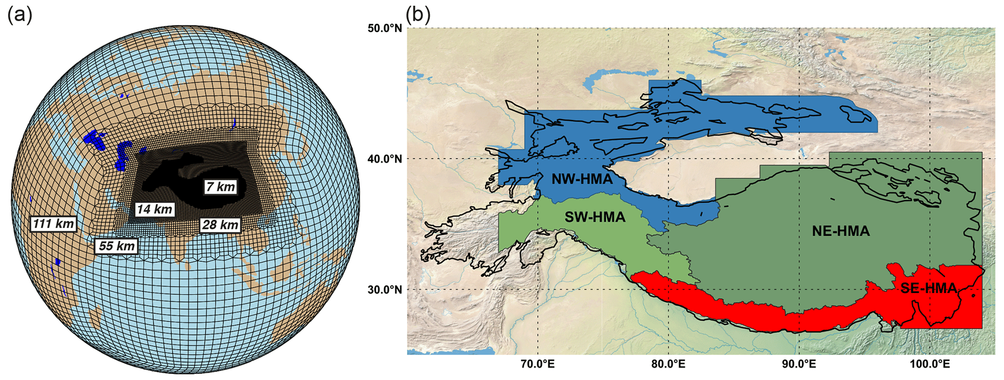
Figure 1(a) Variable-resolution (VR) spectral element (SE) grid developed for this study. (b) Map showing High Mountain Asia (HMA) subregions used to evaluate cryospheric–hydrological variables, along with the outline of HMA. The source of the background imagery in panel (b) is http://naturalearthdata.com/ (last access: 12 April 2022). The HMA subregions are derived from the Randolph Glacier Inventory (RGI) version 6 regions (RGI Consortium, 2017), where SW-HMA (southwest HMA) and SE-HMA (southeast HMA) represent the RGI regions “South Asia West” and “South Asia East”, respectively, and NW-HMA (northwest HMA) and NE-HMA (northeast HMA) represent the RGI region “Central Asia”. The RGI region of “Central Asia” has been split into two subregions to better represent the regional climate characteristics. The HMA outline is derived from the Global Mountain Biodiversity Assessment (GMBA) mountain inventory version 1.2 (Körner et al., 2017).
Three transitional grids with horizontal grid spacings of ∼ 14 km (0.125∘), ∼ 28 km (0.25∘), and ∼ 55 km (0.5∘) serve as a buffer between the HMA domain and the global 1∘ (∼ 111 km) domain. The 0.5∘ grid extends from the Black Sea in the west to the Yellow Sea in the east and from the Indian Peninsula in the south to Siberia in the north. To ensure a smooth transition between varying grid resolutions and numerical stability, the buffer zone spans up to five spectral elements, with spring dynamics used to smooth the grid transition zones and to create nearly orthogonal angles between elements (Guba et al., 2014). The HMA_VR7 grid contains 226 964 horizontal grid points, which is about 4.7 times more than on a globally uniform 1∘ SE grid (48 600 grid points).
To find a balance between computational cost and numerical stability, the CAM-SE time-stepping performance of the HMA_VR7 grid was tested in an Aquaplanet environment, which is a simplified environment that assumes the Earth's surface to be covered by oceans only (Zarzycki et al., 2014). We achieved stability with time steps of 225 and 18.75 s for CAM physics and dynamics, respectively, which are 8 and 16 times smaller than the CAM physics (1800 s) and dynamics (300 s) time steps on a globally uniform 1∘ SE grid. Hyperviscosity coefficients that prevent numerical artifacts and instability are scaled according to the dimensions of a grid element (Guba et al., 2014). For each halving of the grid resolution, the hyperviscosity coefficients decrease by 1 order of magnitude (Zarzycki et al., 2014). The VR-CESM simulations were performed on the supercomputing facility of Cheyenne at the National Center for Atmospheric Research (NCAR). With a computational cost of about 90 000 h per simulated year, the HMA_VR7 grid is about 5 % cheaper than a globally uniform 0.25∘ SE grid (777 600 grid points), which costs about 95 000 h per simulated year, and about 35 times more expensive than a globally unform 1∘ SE grid, which costs about 2500 h per simulated year. Using 1584–2520 processors (44–70 nodes), the throughput of the HMA_VR7 grid is about 0.3–0.7 simulated years per wall-clock day.
The spectral element dynamical core used by CESM is currently based on the hydrostatic approximation; non-hydrostatic vertical acceleration terms are neglected, which are important for the representation of deep convection, gravity waves, and flow over topography (Jeevanjee, 2017; Liu et al., 2022). Conventionally, the horizontal scales at which non-hydrostatic terms become important are assumed to be O(10 km), which is the vertical scale of the troposphere (e.g., Wedi and Smolarkiewicz, 2009). This could raise the question of whether it is appropriate or not to use a 7 km regionally refined grid in combination with a hydrostatic model. In the literature, there is, however, a spread of the grid spacing at which non-hydrostatic dynamics become important. There are, for instance, studies that indicate that non-hydrostatic dynamics are only important for grid spacings finer than 10 km. Jeevanjee (2017) illustrated that in the FV3 model, the non-hydrostatic and hydrostatic vertical velocities only begin to diverge at dx=2 km or finer. Jang and Hong (2016) highlighted prior studies (e.g., Dudhia, 1993, 2014; Kato, 1996; Janjic et al., 2001) indicating that non-hydrostatic dynamics are “weak” at grid spacings coarser than 5 km. Similarly, a study of the Integrated Forecast System (IFS) model using hydrostatic and non-hydrostatic versions found very little sensitivity down to 5 km (Wedi et al., 2010). Other studies indicate that non-hydrostatic dynamics are also important at grid spacings coarser than 10 km, which is suggested by the studies of Yang et al. (2017) and Liu et al. (2022), who show that non-hydrostatic terms are important at grid spacings up to 25 km, particularly in the representation of tropical convective systems. Due to the inherent difficulty in testing the null hypothesis (Liu et al., 2022), and the spread in the literature of the grid spacing at which non-hydrostatic dynamics become important, we believe there are insufficient grounds to deem our model configuration inappropriate. However, we are aware that using the hydrostatic version in combination with a 7 km regionally refined grid could propagate model-related uncertainties into model outputs, such as precipitation. Nonetheless, the ability of the hydrostatic VR-CESM to simulate a mountainous climate with a 7 km regionally refined grid has successfully been shown over the mountain ranges of the western USA (Rhoades et al., 2018).
2.3 Topography and land surface
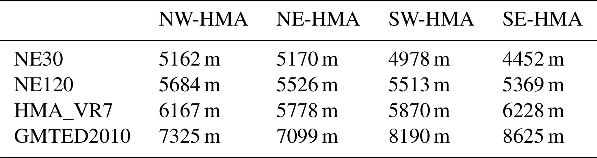
The topography of the HMA_VR7 grid was interpolated from the 30 arcsec (∼ 1 km) Global Multi-resolution Terrain Elevation Data (GMTED2010; Danielson and Gesch, 2011) of the United States Geological Survey (USGS), using an updated version of the NCAR_Topo software package (Lauritzen et al., 2015). The updated software package includes ridge-finding and internal-smoothing algorithms to improve the accuracy of high-resolution topography. Figure 2 shows a snapshot of the topography over western HMA (the Karakoram and upper Indus Basin; 32–37∘ N, 72–78∘ E) for the globally uniform 1 and 0.25∘ SE CESM grids (hereafter NE30 and NE120, respectively, where NE stands for the number of elements in each coordinate direction on a panel; Lauritzen et al., 2018) and for the HMA_VR7 grid and GMTED2010. Compared to NE30 and NE120, the HMA_VR7 topography represents the detailed topography of this region more accurately. Over HMA, the maximum altitude increases from 5170 and 5684 m for NE30 and NE120, respectively, to 6228 m for HMA_VR7. These maxima are observed in the northeastern, northwestern, and southeastern HMA subregions (Fig. 1b), respectively (Table 1).
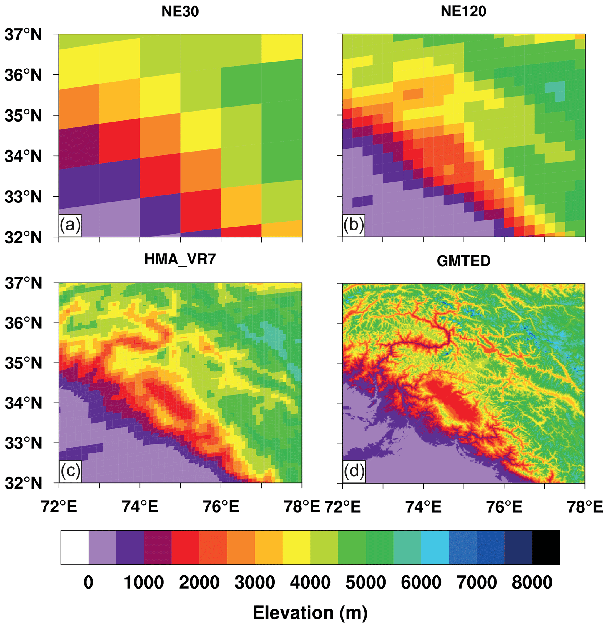
Figure 2Topographical representation of western High Mountain Asia (i.e., upper Indus River and Karakoram mountains; 32–37∘ N, 72–78∘ E) by globally uniform 1 and 0.25∘ CESM grids (NE30 and NE120, respectively) (a–b), the HMA_VR7 grid (c), and a reference dataset, GMTED2010 (Danielson and Gesch, 2011; d).
Table 1Maximum altitude per HMA subregion (Fig. 1b) as observed for NE30, NE120, HMA_VR7, and GMTED2010.
The land surface characteristics of the HMA_VR7 grid are partly transient and partly constant. The distribution of plant functional types (PFTs) is transient; the time series of land use changes are derived and interpolated from the Land-Use Harmonization (LUH2) time series (Hurtt et al., 2020), which covers the period of 1850–2015 and describes annual land use changes based on the History Database of the Global Environment (HYDE version 3.2; Klein Goldewijk et al., 2017). Other land surface classes, such as glaciers and lakes, are assumed to be constant using the distributions of the year 2000 by default.
2.4 VR-CESM simulations setup
We performed two transient model simulations covering a 20-year period, 1979–1998, using the HMA_VR7 grid. Both simulations use several model modifications, including a new glacier region over HMA, with a 36 EC scheme in CLM. The new glacier region makes it possible to simulate SMB in multiple (including virtual) ECs in HMA, while retaining the computationally cheaper default behavior of one EC per grid cell in other mountain glacier regions. The HMA glacier region covers a domain between 20 and 50∘ N and between 55 and 110∘ E.
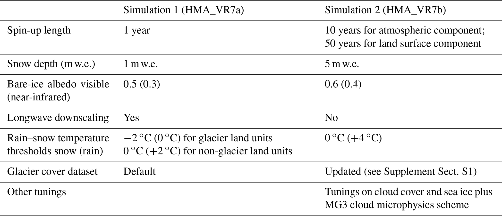
For the first simulation (hereafter HMA_VR7a), the model is spun-up for 1 year. The maximum allowed snow depth (Hmax) is reduced to 1 m w.e. (the default value in CESM1) under the assumption that a 1-year spin-up is not sufficient to reach m w.e. Other CLM settings follow the CESM2 defaults, including a bare-ice albedo of 0.5 (0.3) for the visible (near-infrared) wavebands, the application of longwave downscaling, and rain–snow repartitioning using temperature thresholds of −2 ∘C (0 ∘C) for snow and 0 ∘C (+2 ∘C) for rain over glaciated (non-glaciated) land units. The rain–snow repartitioning is based on downscaled temperature. It uses a linear ramp that assumes that precipitation falls as snow (rain) when the temperature is below (above) the lower (upper) temperature threshold and that precipitation falls as a mix of rain and snow when the temperature is between the two thresholds.
For the second simulation (hereafter HMA_VR7b), the model is initialized with a snow depth of 2.5 m w.e. over glaciated land units, followed by a CAM spin-up of 10 years and a CLM spin-up of 50 years. For the CAM spin-up, CESM is run according to the AMIP protocol, keeping the solar and external forcing, surface emissions, ozone, and volcanic aerosols fixed to the 1979 level. The coupler output of this spin-up is used to initialize CLM, which is run in a standalone mode and with sub-cycles over a 10-year period (i.e., the length of coupler output) for 50 years. A period of 50 years is sufficient to equilibrate the terrestrial system components, such as snowpack. The outputs of the atmospheric and land spin-up are then used to initialize the transient simulation. For HMA_VR7b, we made several model changes to reduce biases compared to HMA_VR7a. These changes include
-
An increase in Hmax from 1 to 5 m w.e. to increase the refreezing capacity.
-
An increase in bare-ice albedo to 0.6 (0.4) for visible (near-infrared) wave bands (i.e., the default values in CESM1) to reduce the ice melt.
-
Modified rain–snow repartitioning temperature thresholds to 0 ∘C for snow and +4 ∘C for rain over all land units, consistent with observed rain–snow temperature thresholds in HMA (Jennings et al., 2018).
-
No downscaling of downward longwave radiation.
-
Tunings of cloud cover and sea ice, including the MG3 cloud microphysics scheme (Gettelman et al., 2019b). This is an update of the MG2 scheme that includes the effects of graupel or hail. The tunings also include
- –
an increase in the strength of the pressure damping (CLUBB C11b) for the third moment of vertical velocity in the large skewness regime from 0.35 to 0.4, to increase low-level cloudiness;
- –
an increase in the microphysical autoconversion size threshold for ice to snow (micro_mg_dcs) from to m; and
- –
an increase in snow grain radius (r_snw) from 1.25 to 1.5 standard deviations and a decrease in snowmelt onset temperature (dt_melt) from 1.5 to 1.0 ∘C to tune shortwave radiation and albedo over sea ice.
- –
-
An updated CLM glacier cover dataset, which is described in more detail in Sect. S1 in the Supplement.
The differences between HMA_VR7a and HMA_VR7b are also listed in Table 2.
Table 2Overview of the modeling setup differences between the first and second HMA VR simulations (HMA_VR7a and HMA_VR7b, respectively).
2.5 Reference data
To evaluate the HMA VR simulations, we compare the gridded outputs with outputs from an NE30 CESM run that covers the same 20-year period (1979–1998). We use the following (re)analysis, observation-based, and satellite-derived products and WRF-based output:
-
The ERA5 reanalysis (Hersbach et al., 2020) is used to evaluate geopotential height and air temperature over the period 1979–1998. ERA5 is available at a spatial resolution of , at monthly intervals, and at 37 pressure levels.
-
The WFDEI dataset (Weedon et al., 2014) is used to evaluate 2 m temperature, rainfall, and snowfall for 1979–1998. WFDEI stands for Watch Forcing Data methodology applied to ERA-Interim data. The dataset has a spatial resolution of 0.5∘ × 0.5∘ and uses ERA-Interim output that is corrected for elevation using environmental lapse rates (i.e., for temperature). The data are bias-corrected using gridded observations from datasets developed by the Climate Research Unit (CRU) or the Global Precipitation Climatology Centre (GPCC). In this study, we used the WFDEI datasets that are bias-corrected based on GPCC and are available at monthly intervals.
-
Northern Hemisphere (NH) snow cover extent from the National Snow and Ice Data Center (NSIDC; Brodzik and Armstrong, 2013) is used to evaluate snow cover for 1979–1998. The NSIDC snow cover data are available on a 25×25 km EASE 2.0 grid at weekly intervals. To enable the evaluation of monthly model output, the weekly NSIDC snow cover data are converted to monthly intervals.
-
The High Asia Refined analysis version 2 (HAR v2; Wang et al., 2021) is used to evaluate snow depth. HARv2 is based on Weather Research and Forecasting (WRF) simulations that are dynamically downscaled with ERA5 and is available on a 10×10 km grid at monthly intervals. The snow depth in HARv2 is corrected with snow depth from the Japanese 55-year reanalysis (Kobayashi et al., 2015), which has shown good performance compared to other global reanalysis datasets in simulating snow depth (Orsolini et al., 2019). Since HARv2 data are not available for 1979, we only evaluate the model output for the period 1980–1998.
-
The Japanese 55-year reanalysis (JRA-55; Kobayashi et al., 2015) is used to evaluate surface energy balance components, including all-sky shortwave and longwave surface radiation fluxes and latent, sensible, and ground heat fluxes for 1979–1998. JRA-55 is available on a T319 Gaussian grid at monthly intervals.
-
The Clouds and Earth's Radiant Energy Systems (CERES) Energy Balanced and Filled (EBAF) dataset (Loeb et al., 2018; Kato et al., 2018) is used to evaluate shortwave cloud forcing and all-sky shortwave and longwave surface radiation fluxes for 1979–1998. The dataset is available on a 1∘ × 1∘ grid at monthly intervals. To evaluate the model output over a similar period (20 years), we use CERES-EBAF data covering the period 2001–2020.
-
Glacier SMB is evaluated for 1979–1998, based on two data sources:
- –
Area-weighted specific mass change rates derived from glaciological and geodetic observations (Zemp et al., 2019). The observation-based mass change rates are regional estimates based on the RGI regions of Central Asia, South Asia West, and South Asia East.
- –
Gridded 1∘ × 1∘ SMB outputs from a glacier mass balance gradient model (Kraaijenbrink et al., 2017) forced by temperature and precipitation fields from the Weather Research and Forecasting (WRF) model (de Kok et al., 2020). The gridded SMB outputs are not available for 1979 and only cover the period 1980–1998.
To allow a uniform comparison among the different CESM grids and the (re)analysis and satellite-based datasets, the CESM output and reference data (e.g., WFDEI, NSIDC, HARv2, JRA-55, CERES-EBAF, and ERA5) are regridded to a 1∘ finite-volume grid, unless noted otherwise.
- –
3.1 Northern Hemisphere atmosphere
Before evaluating the model's ability to simulate cryospheric–hydrological variables such as the glacier SMB, we evaluate its ability to simulate the Northern Hemisphere atmosphere. To this end, we compare the geopotential height and air temperature variables simulated by the different CESM grids, using ERA5 output as a reference. Figure 3 shows the lower tropospheric (500–1000 hPa) eddy geopotential thickness in winter and the upper tropospheric (500–200 hPa) mean temperature in summer (the surface of the Tibetan Plateau lies at about 500 hPa). The lower tropospheric eddy geopotential thickness in the left column of Fig. 3 shows the model's ability to simulate stationary wave patterns. The eddy thickness simulated by the NE30 and HMA VR configurations shows many similarities with the ERA5 output, along with some small differences. Both the CESM output and ERA5 output have a stationary wave pattern over the Northern Hemisphere, with two negative eddy thickness centers over Siberia and Canada and two positive eddy thickness centers over the North Pacific and the North Atlantic. The negative eddy centers have a similar shape and magnitude, whereas the positive centers are similar in shape with small differences in magnitude. NE30 is more similar to ERA5 over the North Pacific, whereas the HMA VR configurations are more similar to ERA5 over the North Atlantic.
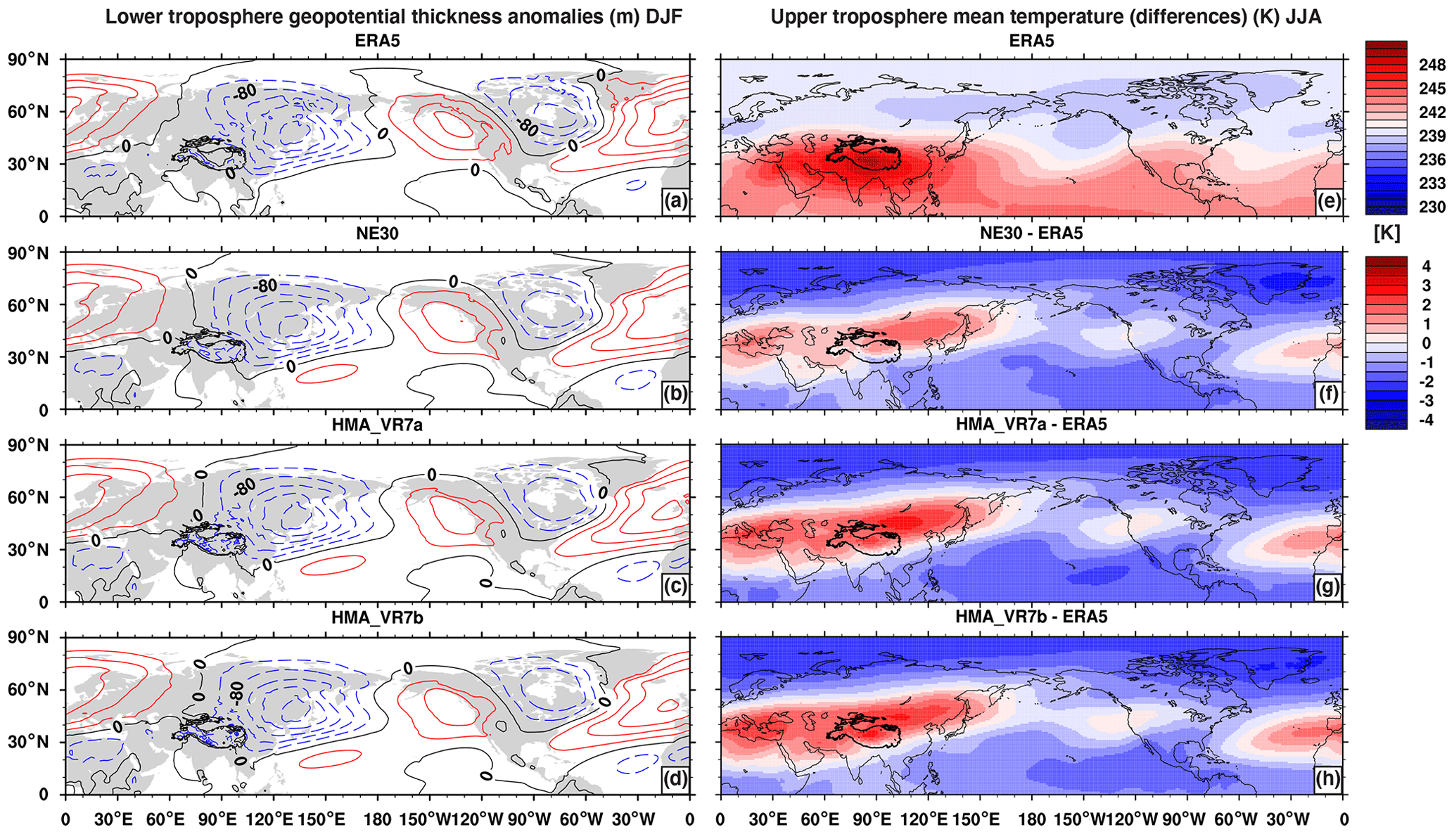
Figure 3(a–d) Northern Hemisphere lower troposphere eddy of the 500–1000 hPa geopotential thickness (m) in winter (December–February, DJF) for ERA5 (a), NE30 (b), HMA_VR7a (c), and HMA_VR7b (d). (e–h) Northern Hemisphere upper troposphere (200–500 hPa) summer (June–August, JJA) mean temperature (K) for ERA5 (e) and the temperature differences relative to ERA5 for NE30 (f), HMA_VR7a (g), and HMA_VR7b (h).
The upper tropospheric summer temperature biases (relative to ERA5) can help us to understand the effects of atmospheric biases on temperature-sensitive surface variables such as ice melt and snowmelt. However, atmospheric biases do not necessarily need to correspond with surface temperature biases, as we will show in Sect. 3.3. Compared to ERA5, NE30 shows an elongated warm anomaly over the midlatitudes, with the largest warm bias (about +2 K) over Mongolia and northern China. The HMA VR configurations show a similar pattern but with a larger warm bias (about +3 K), which is likely related to its higher horizontal resolution. This is a known issue in GCMs and ESMs, particularly at midlatitudes (Roeckner et al., 2006; Herrington and Reed, 2020). One explanation is that increasing horizontal resolution leads to larger resolved vertical velocities and increased condensational heating. This heating, computed in the macrophysics routine of CLUBB, especially raises upper tropospheric temperature at midlatitudes (Herrington and Reed, 2020).
3.2 Cloud forcing
Figure 4 shows the model's annual mean shortwave cloud radiative (SWCF) forcing biases relative to the CERES-EBAF product. The SWCF quantifies the impact of clouds on incident shortwave and is computed as the difference between all-sky and clear-sky shortwave radiative fluxes at the top of the atmosphere. NE30 shows biases typical of CESM2, with positive biases near the marine stratocumulus decks off the coast of the southwestern USA. The HMA_VR7a simulation has larger biases than NE30, with more positive biases almost everywhere in the Northern Hemisphere, indicating thinner clouds. This reduction in cloud thickness is primarily due to the smaller physics time step in the HMA configurations. HMA_VR7b was tuned to remove this sensitivity to the physics time step, resulting in a SWCF bias that looks more similar to the NE30 run (Fig. 4b). However, the positive SWCF biases over HMA remain in HMA_VR7b.
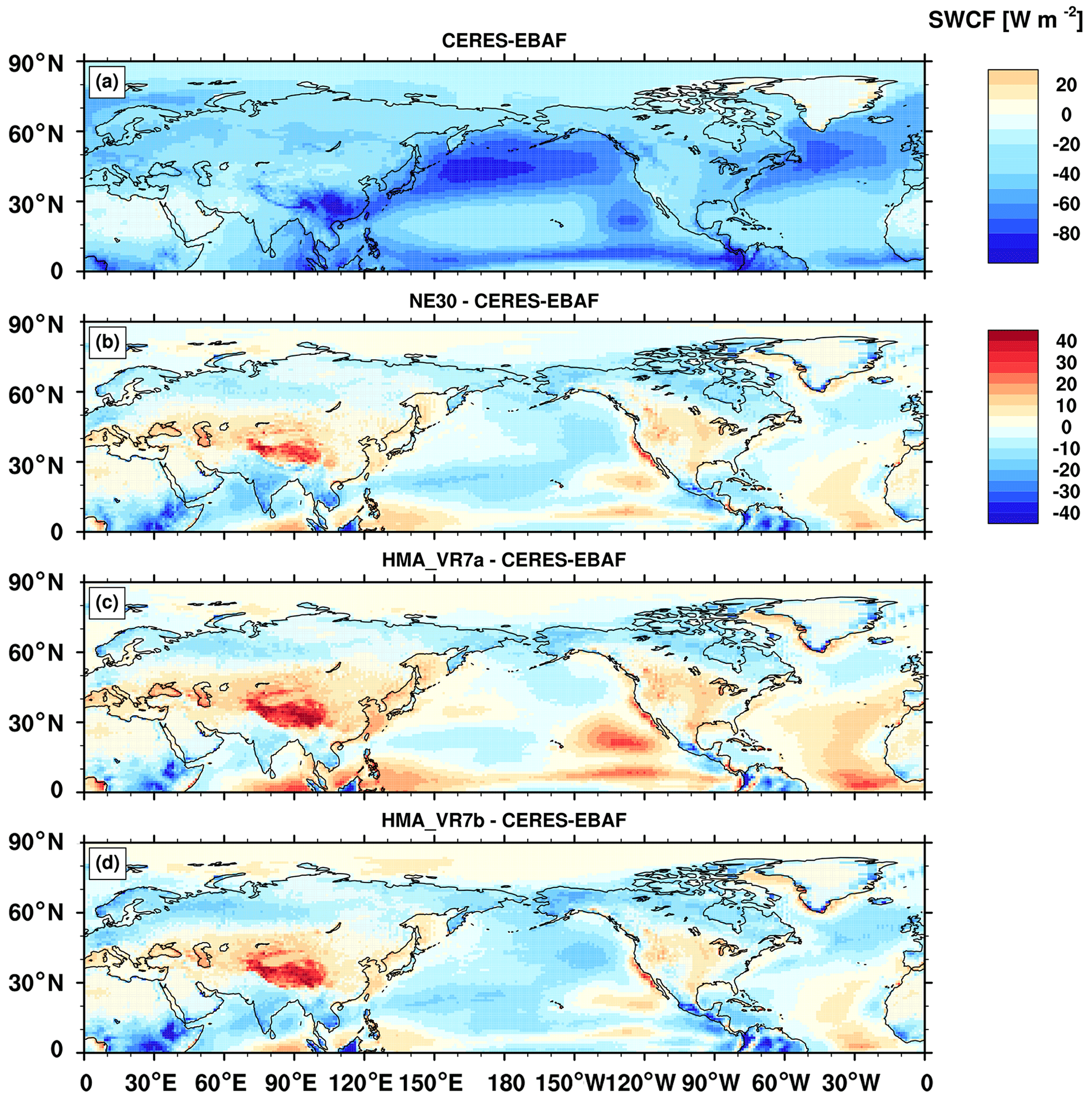
Figure 4Northern Hemisphere annual mean shortwave cloud forcing (W m−2) from CERES-EBAF (a) and model biases relative to CERES-EBAF (b–d) for NE30 (b), HMA_VR7a (c), and HMA_VR7b (d). All differences are computed after mapping model fields to the CERES-EBAF 1∘ grid.
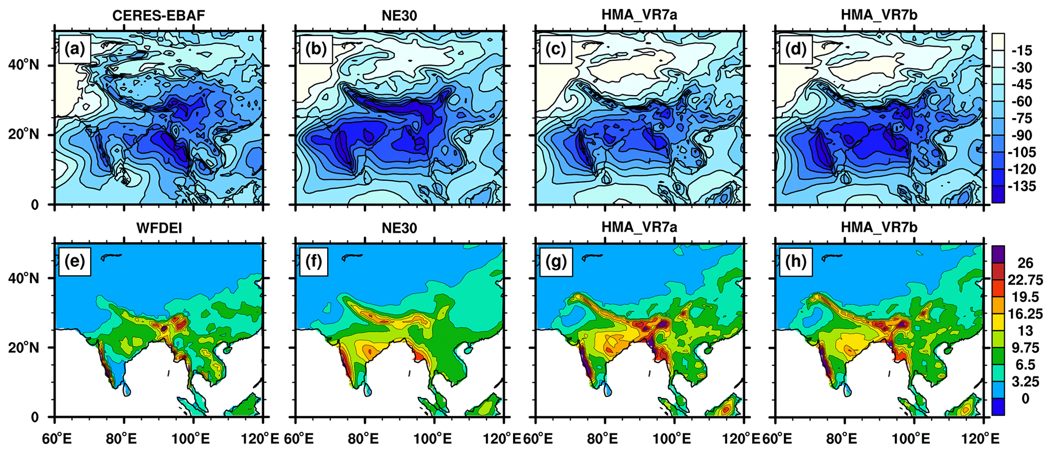
Figure 5Northern Hemisphere summer climatological (a–d) shortwave cloud forcing (W m−2) and (e–h) precipitation rate (mm d−1) in observations and models. (a) CERES-EBAF, (b, f) NE30, (c, g) HMA_VR7a, (d, h) HMA_VR7b, and (e) WFDEI precipitation rates. Top row shows fields mapped to the CERES-EBAF 1∘ grid, and the bottom row shows fields mapped to the NE30 grid.
Figure 5 shows the summer mean SWCF, which contributes to summer melting. The clouds over the Himalayan front range are too expansive in NE30 compared to CERES-EBAF, spanning hundreds of kilometers in the north–south direction. The HMA VR configurations instead produce a narrow SWCF feature over the front range that is more similar to the observations (Fig. 5a). However, the clouds have mostly disappeared from the northern half of the Tibetan Plateau compared to the NE30 control and CERES-EBAF, as also shown in the annual mean plots in Fig. 4. Our cloud tunings in HMA_VR7b are therefore unable to restore the clouds locally over the Tibetan Plateau. The VR model's inability to produce realistic mean cloud states inside and outside the refined region is a major limitation of the variable-resolution method (Rauscher et al., 2013).
The bottom panel of Fig. 5 shows the summer mean precipitation rates over HMA in the models and the WFDEI validation product. NE30 does not capture the intensity and location of the summer precipitation patterns, in particular over the west coast of India and the eastern side of the Himalayas, which extend southward to the eastern coasts of Bangladesh and Burma. In contrast, the HMA VR configurations improve the intensity and location of these features, indicating more realistic monsoonal rainfall.
To explore the causes of the cloud and precipitation changes in the HMA VR runs, Fig. 6 shows latitude–height transects averaged over the longitude band 80–100∘. The monsoonal circulation in the NE30 run has two centers, namely a broad region of ascent in the southern HMA region, primarily over the Indian Ocean, and a narrower region of ascent over the front range of the Himalayas (Fig. 6d). These ascent centers are co-located with condensational heating from CLUBB (Fig. 6g), which sustains the monsoonal circulation. In the HMA VR runs, the ascending center associated with the front range is displaced south, merging with the southern ascent center and manifesting as a single, broad region of ascent (Fig. 6e–f). This new circulation is more intense than the NE30 circulation, as shown by a broad region of anomalous condensational heating upwind of the front range (Fig. 6h–i) and coinciding with the larger mean precipitation rates in Fig. 5.
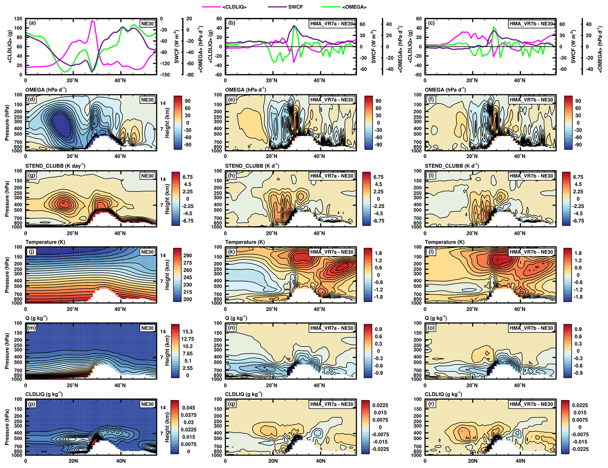
Figure 6Northern Hemisphere summer climatological mass fraction of cloud liquid amount (CLDLIQ; g kg−1), shortwave cloud forcing (SWCF; W m−2), vertical velocity (OMEGA; hPa d−1), CLUBB condensational heating (STEND_CLUBB; K d−1), air temperature (K), and specific humidity (Q; g kg−1) in a latitude–height transect averaged over 80–100∘ longitude. NE30 (left column), HMA_VR7a differences relative to NE30 (middle column), and HMA_VR7b differences relative to NE30 (right column) are shown.
The anomalous ascent on the southern side of the mountains is balanced by the anomalous descent on the northern side of the plateau (Fig. 6e–f). This anomalous descent likely explains the increased temperatures (Fig. 6k–l), reduced humidity (Fig. 6n–o), and reduced cloudiness (Fig. 6q–r) on the northern side of the plateau, as these are all consistent with a subsiding environment. While the warming and drying patterns are largely the result of greater vertical velocities due to the enhanced spatial resolution in the HMA VR runs, the shorter physics time step also contributes to this warming and drying (not shown).
3.3 Surface temperature and precipitation
Whereas the summer tropospheric temperature over HMA rises with increasing horizontal resolution, the near-surface (2 m) temperature falls. Figure 7 shows the 2 m temperature differences and pattern correlations between the NE30 and HMA VR simulations and the observation- and reanalysis-based WFDEI for each season. The differences are shown over the four HMA subregions (Fig. 1b) and the pattern correlations for the domain (20–50∘ N, 65–105∘ E). During summer (June–August, JJA), NE30 has a warm temperature bias (relative to WFDEI) up to ∼ 2.5 ∘C (here and hereafter the numbers in parentheses refer to a bias representing the median bias) over all HMA subregions. This bias decreases with increasing resolution. For HMA_VR7, the JJA warm bias is present only in northern HMA (up to ∼ 2.5 ∘C), whereas southern HMA has a cold bias relative to WFDEI (up to ∼ 2 ∘C). During winter (December–February, DJF), spring (March–May, MAM), and autumn (September–November, SON), cold biases are present over SW-HMA (the region including the Karakoram and Hindu Kush mountain ranges), growing larger (up to ∼ 8 ∘C) with increasing resolution. Over other HMA subregions, cold biases are also present but are smaller (up to ∼ 2 ∘C). The cold temperature biases could partly be a result of uncertainties in WFDEI. Since WFDEI is bias-corrected using gridded observations of GPCC, the accuracy of the data relies on the availability of meteorological measurements that are scarce in High Mountain Asia, especially at higher altitudes and in the more remote domains of HMA. The lack of measurements could result in temperature overestimates and precipitation underestimates (Lalande et al., 2021; Gu et al., 2012; Palazzi et al., 2015; Immerzeel et al., 2015), which can to some extent explain the cold temperature biases and, as we will show later, the wet precipitation biases that are visible in the NE30 and HMA VR simulation outputs.
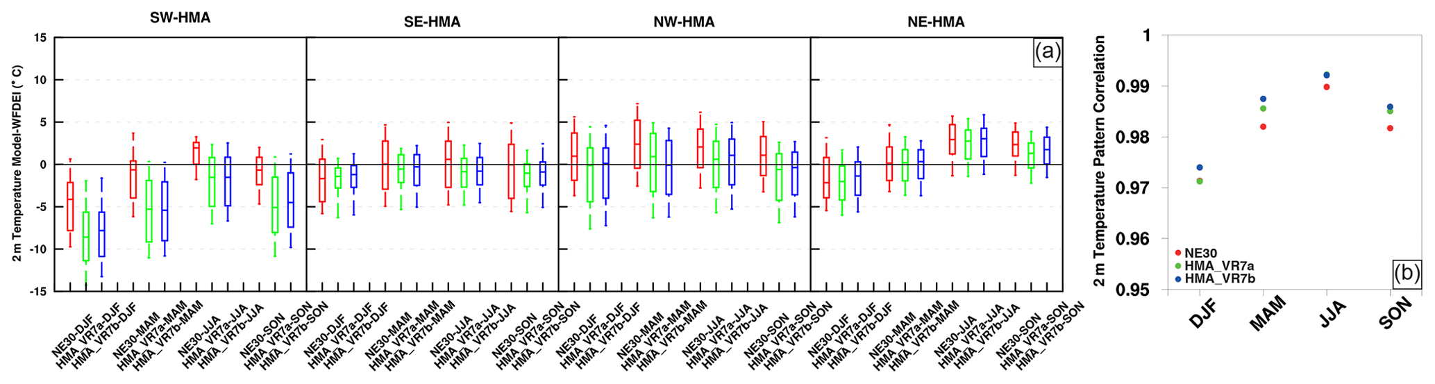
Figure 7(a) Box plots of 2 m temperature differences (∘C) between the simulation outputs of NE30 (red), HMA_VR7a (green), HMA_VR7b (blue), and the observation- and reanalysis-based WFDEI for each season and HMA subregion (shown in Fig. 1b). The box represents the biases between the 25th and 75th percentiles, the line in the box denotes the median, and the whiskers represent the 10th and 90th percentiles of temperature differences. (b) Pattern correlations between the simulation outputs of NE30 (red), HMA_VR7a (green), HMA_VR7b (blue), and the observation- and reanalysis-based WFDEI. The pattern correlations are calculated for each season and for the entire HMA region.
The contrary temperature response between the atmosphere (increasing temperature with finer resolution) and land surface (decreasing temperature with finer resolution) can be explained by a combination of better-resolved topography and multiple elevation classes for the fine grids. Whereas the NE30 runs have a single EC, the VR runs have 36 ECs for HMA glaciers. With multiple ECs, the atmospheric temperature received from CAM is downscaled with altitude over glaciated land units, which can lower the grid cell mean temperature in highly glaciated regions where glaciers lie above the grid cell mean elevation. The bias difference between NE30 and HMA_VR7 is especially prominent in SW-HMA, which is the most glaciated subregion. The pattern correlations between WFDEI and CESM as shown in Fig. 7b are above 0.95, with the highest correlations in JJA and for HMA_VR7b. This suggests that CESM is able to simulate spatial temperature patterns that agree with the observation- and reanalysis-based patterns shown by WFDEI.
Figure 8 shows the monthly mean precipitation (rainfall and snowfall) differences and pattern correlations for the NE30 and HMA VR simulations and WFDEI. Rainfall is overestimated relative to WFDEI during JJA in southern HMA (up to ∼ 150 mm per month), particularly in SE-HMA, which is monsoon-dominated and the wettest HMA subregion with summer rainfall sums of 740 mm in WFDEI (Table S2). The interquartile range of the rainfall bias is similar among the CESM grids, whereas the median of the rainfall bias is slightly larger for NE30 than for HMA VR in most subregions. The pattern of correlation between WFDEI and CESM is worse during DJF, with correlations of 0.87–0.90, and best during SON, with correlations of 0.93–0.96. The best-performing grid relative to WFDEI varies per season; NE30 is better in DJF, and HMA_VR7 is better in the other seasons. Snowfall is overestimated in the southern HMA subregions during DJF and MAM (up to ∼ 50 mm per month), particularly in SW-HMA, where winter snowfall sums up to 99 mm in WFDEI (Table S2). The snowfall bias is generally largest for HMA_VR7b, followed by HMA_VR7a and NE30. The snowfall bias is likely related to the cold bias in this region (Fig. 7) and to some extent to the changed rain–snow repartitioning temperature thresholds in HMA_VR7b, which favor snowfall. The snowfall (and rainfall) biases could also be a result of the aforementioned uncertainties in WFDEI. Although the snowfall biases are large during DJF and MAM, the pattern correlations suggest that CESM, with correlations of 0.8–0.86, can reasonably simulate the snowfall patterns of WFDEI, with HMA_VR7 performing better than NE30. Only in JJA do the simulated snowfall patterns show a large deviation from the WFDEI snowfall patterns. The NE30 run has the worst performance, with a pattern correlation of 0.37. The HMA_VR7 grid gives pattern correlations of 0.68–0.7, which are consistent with the improved precipitation shown in Fig. 5.
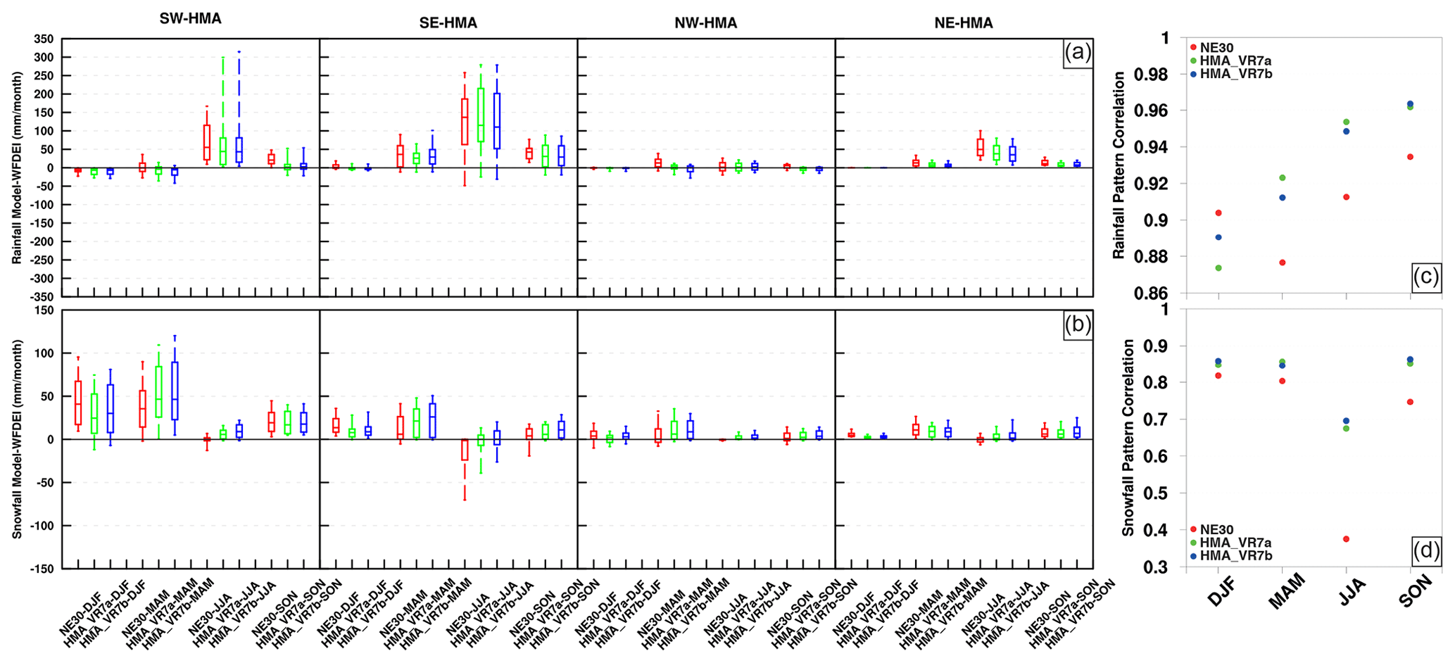
Figure 8Same as Fig. 7 but for rainfall (mm per month) (a–c) and snowfall (mm per month) (b–d).
3.4 Snow depth and cover
Figure 9 shows the monthly mean snow cover and snow depth differences and pattern correlations between the NE30 and HMA VR configurations, the observation-based NSIDC dataset, and the analysis-based HARv2 dataset. In most HMA subregions, snow cover is overestimated during winter (up to ∼ 40 %) and underestimated during summer (up to ∼ 40 %). Only in NE-HMA is the NE30 and HMA VR snow cover comparable to the NSIDC snow cover. The HMA VR simulations show some improvements compared to NE30 during spring and summer, but there are no significant differences between HMA_VR7a and HMA_VR7b. The pattern correlations between the NSIDC data and the NE30 and HMA VR runs are worst during JJA, with correlations of 0.69–0.72, and best during DJF, with correlations of 0.88–0.92. In general, HMA_VR7b has the best snow cover, followed by HMA_VR7a and NE30. Compared to HARv2, snow depth is particularly overestimated over SW-HMA during winter and spring (up to ∼ 100 mm w.e.), in part because of the cold bias. The snow depth from HMA_VR7a has a smaller bias than NE30, but the snow depth from HMA_VR7b shows a larger bias than HMA_VR7a. The increased bias is likely related to the snow model modifications in HMA_VR7b, including a higher maximum snow depth and changed rain–snow repartitioning thresholds. The pattern correlations show a better performance of NE30 and HMA_VR7 during winter and spring than during summer and autumn. In particular, HMA_VR7b underperforms relative to HARv2.
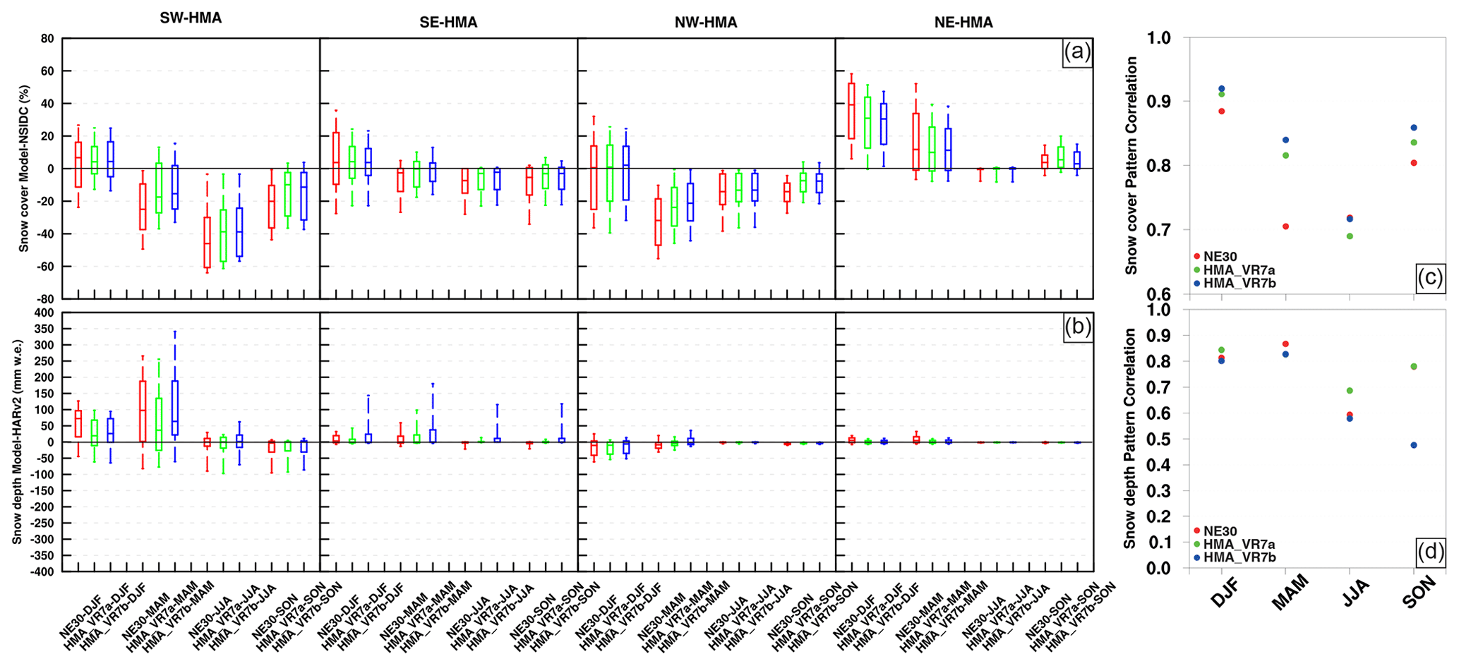
Figure 9Same as Fig. 7 but for snow cover (%) (a–b) and snow depth (mm w.e.) (c–d). The snow cover and snow depth differences are calculated between the CESM simulation output (i.e., NE30, HMA_VR7a, and HMA_VR7b) and snow cover derived from NSIDC and snow depth derived from HARv2, respectively.
3.5 Surface energy balance
Figure 10 shows the annual cycle of surface-energy-balance (SEB) components over glaciated grid cells (encompassing all land units) in HMA. The downwelling, upwelling, and net shortwave radiation (SWd, SWu, and SWnet, respectively) for NE30 and HMA_VR7 are overestimated relative to CERES-EBAF but generally are closer to JRA-55 (Fig. 10a–c; Table 3). SW radiation fluxes are higher for HMA_VR7 than for NE30. The downwelling and upwelling longwave radiation (LWd and LWu, respectively) for NE30 and HMA_VR7 are generally underestimated relative to CERES-EBAF, particularly in winter (Fig. 10d–e; Table 3). In summer, the LWu simulated by HMA_VR7 agrees more closely with CERES-EBAF than NE30 and JRA-55, whereas the LWd is more accurately simulated by NE30 (relative to CERES-EBAF; Table 3). The net LW radiation (LWnet) is underestimated relative to CERES-EBAF, while NE30 is in a closer agreement with CERES-EBAF than HMA_VR7 (Fig. 10f; Table 3). The differences in SW and LW radiation fluxes among the different grids and reference output are likely related to differences in cloud cover. As described in Sect. 3.2, the cloud cover in CESM is too low, especially over the Tibetan Plateau and in the VR runs. With reduced cloud cover, more solar radiation reaches the surface, and less thermal radiation is absorbed, increasing SWd and reducing LWd. The reduced cloud cover can also contribute to the cold biases, especially during wintertime when the net radiation is already negative (Table 3). On a daily basis, reduced cloud cover could result in more shortwave insolation during the day and enhanced radiative cooling during the night when the radiative balance is negative. The enhanced radiative cooling could then eventually lead to a (more) negative net daily radiative balance, especially during wintertime when the nights are longer and the solar inclination angle is lower. Consequently, the surface temperature decreases, contributing to a cold bias.
Table 3Mean annual (ANN), wintertime (DJF |; in italics), and summertime (JJA; in italics) surface energy balance (SEB) fluxes (W m−2) for NE30, HMA_VR7a (HMA1), HMA_VR7b (HMA2), JRA-55, and CERES-EBAF (C-EBF). SEB fluxes are defined as being positive towards the surface and represent the mean fluxes in glaciated grid cells (encompassing all land units) averaged over the entire HMA region and the periods 1979–1998 (for NE30, HMA_VR7a, HMA_VR7b, and JRA-55) and 2001–2020 (for CERES-EBAF).
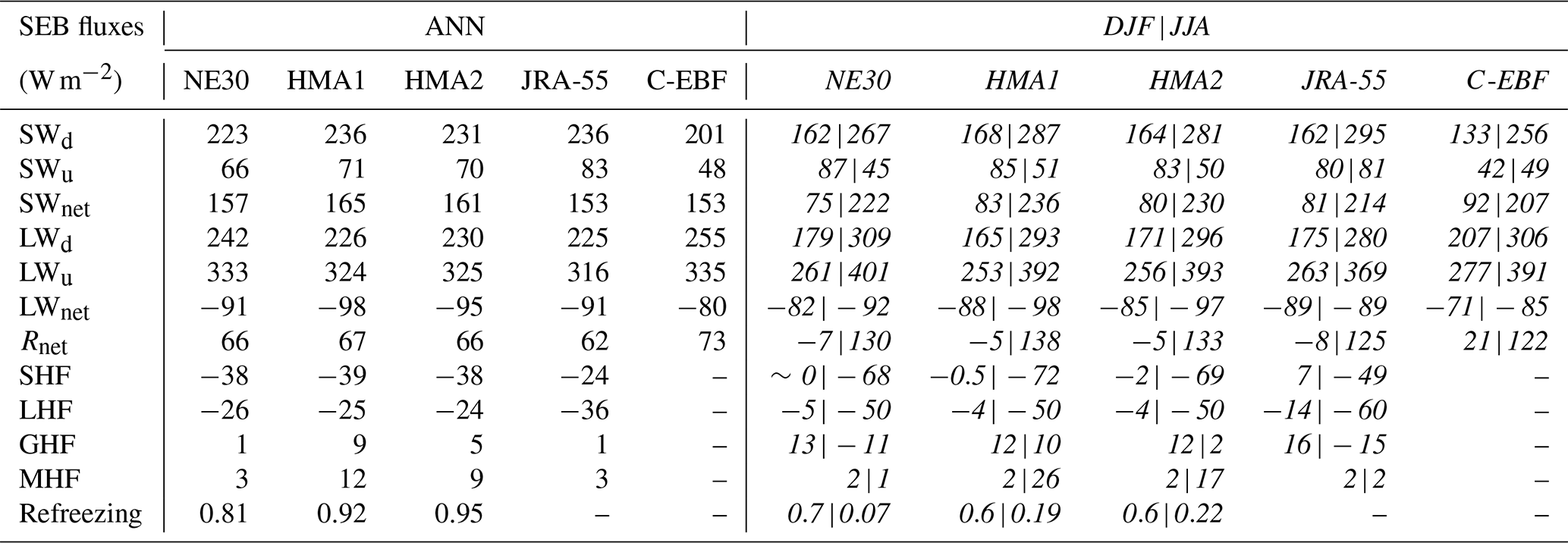
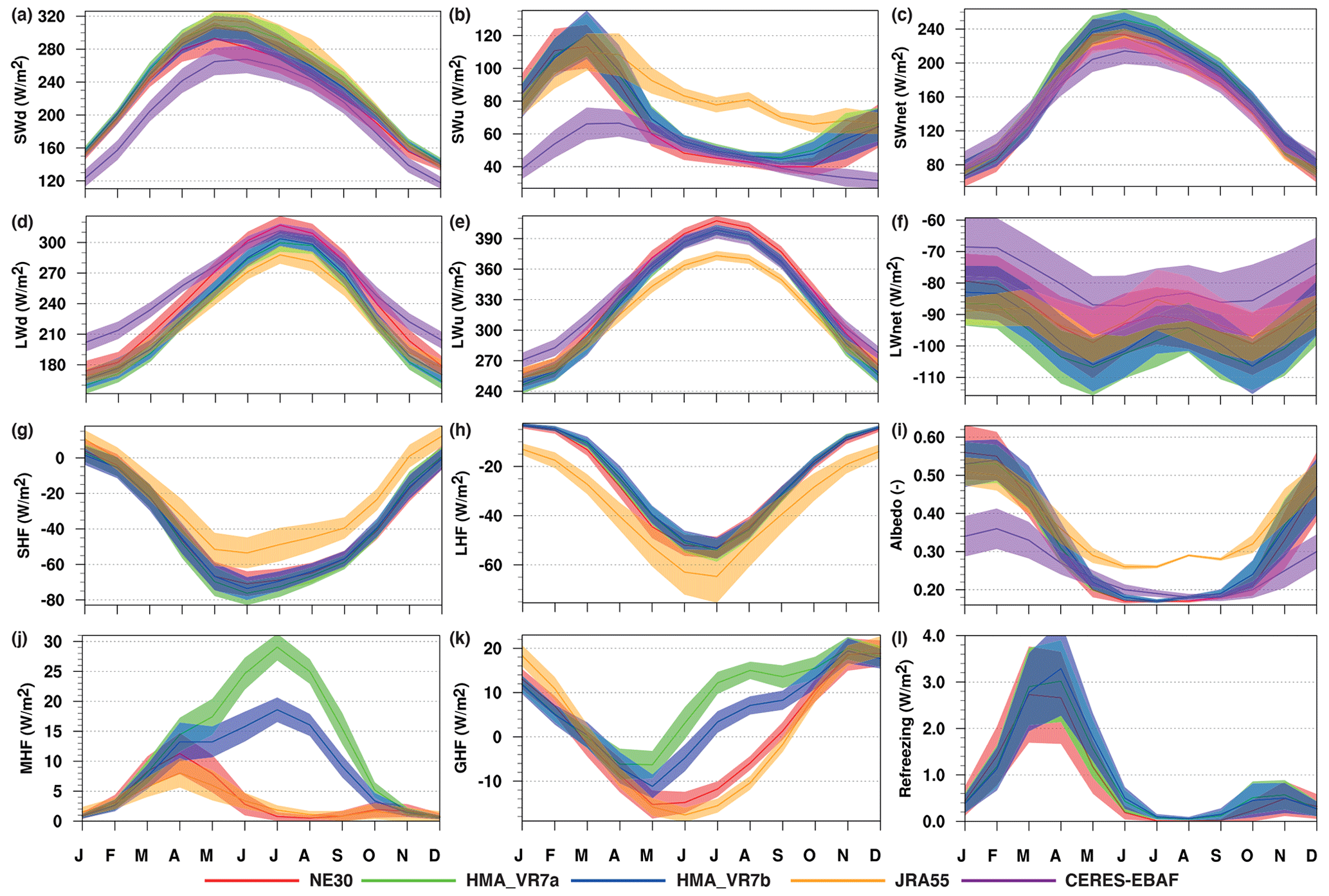
Figure 10Annual cycle of (a) downwelling shortwave radiation (SWd), (b) upwelling shortwave radiation (SWu), (c) net shortwave radiation (SWnet), (d) downwelling longwave radiation (LWd), (e) upwelling longwave radiation (LWu), (f) net longwave radiation (LWnet), (g) sensible heat flux (SHF), (h) latent heat flux (LHF), (i) albedo, (j) melt heat flux (MHF), (k) conductive or ground heat flux (GHF), and (l) refreezing heat flux. The annual cycle of the various SEB fluxes (W m−2) is representative of glaciated grid cells (encompassing all land units) in HMA over the periods 1979–1998 for NE30 (red), HMA_VR7a (green), HMA_VR7b (blue), and JRA-55 (orange) and 2001–2020 for CERES-EBAF (purple). The shading denotes the standard deviation in time, and SEB fluxes are defined as being positive towards the surface.
The seasonal cycle of the sensible and latent heat flux is compared only to JRA-55. In summer, the upward sensible heat flux (SHF) is higher for NE30 and HMA_VR7 than for JRA-55, whereas the upward latent heat flux (LHF) is lower (Fig. 10g–h; Table 3). These biases could be caused by lower snow cover and the subsequent lower sublimation and evapotranspiration. Summer surface albedo is lower for NE30 and HMA_VR7 than for JRA-55 (Fig. 10i) but is in closer agreement with CERES-EBAF. In winter, the surface albedo for NE30 and HMA_VR7 is overestimated relative to JRA-55 and CERES-EBAF, which could be linked to the overestimated snow depth (Fig. 9).
The melt heat flux (MHF; Fig. 10j; Table 3) is higher during summer for HMA_VR7 than for NE30 or JRA-55. Here, HMA_VR7a has a higher MHF than HMA_VR7b, with more ice melt in summer. The greater cloud cover in HMA_VR7b (relative to HMA_VR7a) reduces SWd at the surface and increases LWd, which results in lower net radiation (i.e., the sum of SWnet and LWnet) and reduced melting and heating overall. NE30 and JRA-55 have a lower summer MHF than HMA_VR7 because they are unable to simulate ice melt over High Mountain Asia.
The conductive or ground heat flux (GHF; Fig. 10k; Table 3) simulated by JRA-55 and NE30 is positive in autumn–winter and negative in spring–summer, whereas the GHF simulated by HMA_VR7 is negative only during spring and strongly positive during the other seasons. Here, GHF is positive for heat conduction from the bedrock toward the surface, which usually occurs when the surface is colder than the layers below (van Kampenhout et al., 2020). GHF is typically positive during winter, at night, or after the refreezing of snowmelt and negative during spring–summer and daytime. The combination of a positive winter GHF partly countering the negative radiative balance and latent and sensible heat fluxes close to zero (Table 3) could trigger a so-called stability-induced cooling feedback (Slater et al., 2001). Via the stability-induced cooling feedback, radiative cooling is enhanced, causing the surface temperature to be lower than the overlying air temperature (i.e., a decoupling of the surface from the atmosphere), which could eventually also explain the cold biases. The positive summer GHF simulated by HMA_VR7 is likely not related to the refreezing of snowmelt (which is highest in spring and limited during summer; see Fig. 10l and Table 3) but rather to extensive ice melt, which requires heat extraction from the environment and, in turn, also can contribute to cold biases. Greater MHF for HMA_VR7a than for HMA_VR7b requires a more positive summer GHF. Positive GHF is also observed over the ablation zones of the Greenland ice sheet (GrIS), although this is likely related to high rates of snow refreezing (van Kampenhout et al., 2020).
3.6 Surface mass balance
Figure 11 shows the area-averaged glacier surface mass balance derived from geodetic and glaciological observations, WRF-based output, and the HMA VR simulations for three Randolph Glacier Inventory (RGI) regions, namely Central Asia (NE-HMA and NW-HMA), South Asia West (SW-HMA), and South Asia East (SE-HMA). The observation- and WRF-based SMBs are in the same range (between +0.5 and −0.5 m w.e. yr−1), whereas the SMB of HMA_VR7 is too negative. The SMB bias is larger for HMA_VR7a, with SMB values of −2.5 to −4.0 m w.e. yr−1. HMA_VR7b shows significant improvement, with SMB values from −0.5 to −2.5 m w.e. yr−1.
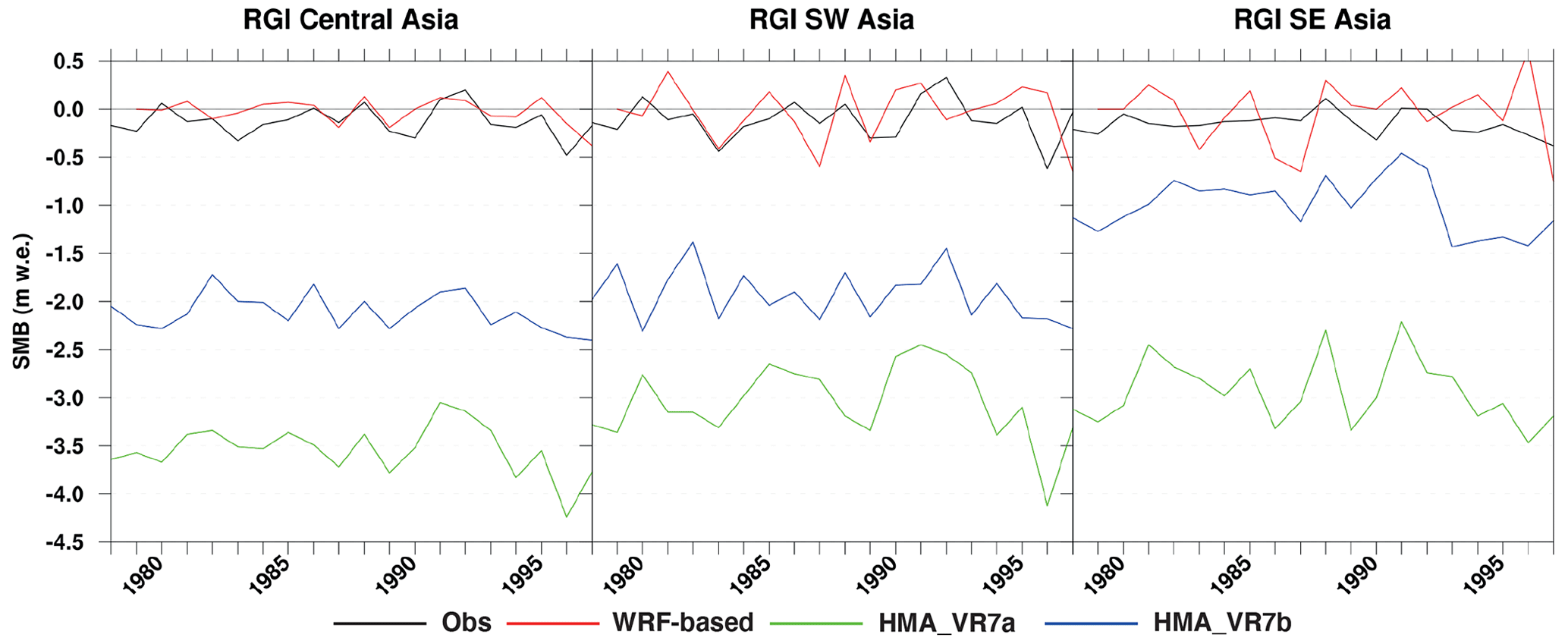
Figure 11Area-averaged annual SMB (m w.e. yr−1) over the period 1979–1998, as derived from geodetic and glaciological observations (Zemp et al., 2019; Obs; black), gridded outputs from a glacier model forced by WRF output (de Kok et al., 2020; WRF based; red), and simulation outputs of HMA_VR7a (green) and HMA_VR7b (blue). The area-averaged annual SMB is calculated for three different regions, namely the RGI region of Central Asia, which includes the HMA subregions NW-HMA and NE-HMA (Fig. 1), and the RGI regions of SW Asia and SE Asia, which represent HMA subregions SW-HMA and SE-HMA, respectively (Fig. 1).
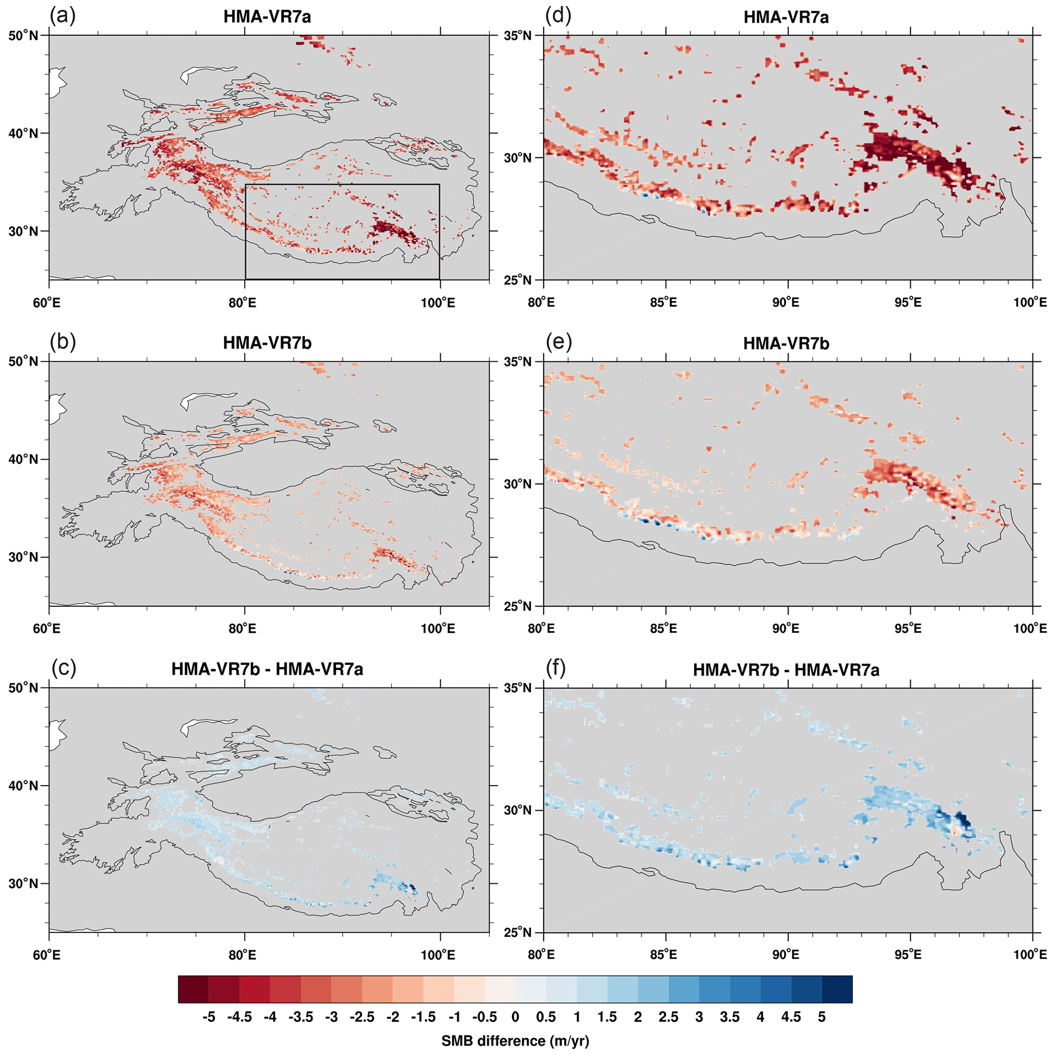
Figure 12Spatial distribution of mean annual SMB (m w.e. yr−1) over the period 1979–1998, as simulated by HMA_VR7a (a–b) and HMA_VR7b (c–d), and the SMB differences between the two simulations (e–f). The black box in panel (a) denotes the area (25–35∘ N; 80–100∘ E) of the insets over the southeastern HMA (d–f). The HMA outline is derived from the Global Mountain Biodiversity Assessment (GMBA) mountain inventory version 1.2 (Körner et al., 2017).
SMB improvements over southern and southeastern HMA are also visible in Fig. 12, which shows the spatial distribution of mean annual SMB (m w.e. yr−1) for 1979–1998, as simulated by HMA_VR7a and HMA_VR7b. The SMB for HMA_VR7a is mostly negative, except for a few small regions in southernmost HMA where a positive SMB is simulated (Fig. 12a, b). The positive SMB in these regions can likely be attributed to high monsoon precipitation. The SMB is mostly negative in southeastern HMA, in part because of inaccuracies in the original glacier cover dataset. The SMB for HMA_VR7b is less negative for the majority of glaciated grid cells, with the greatest improvements in southeastern HMA (Fig. 12c–f), where the updated glacier cover dataset is based on more accurate glacier outlines and includes glaciers located at altitudes between than 6000 and 7000 m. Glaciers at these altitudes generally have a more positive SMB than lower-altitude glaciers (Fig. 13). Also, HMA_VR7b has more grid cells with a positive SMB, especially in SE-HMA. Compared to HMA_VR7a, the number of grid cells with a positive SMB at the end of a model run nearly triples (from 105 to 299).
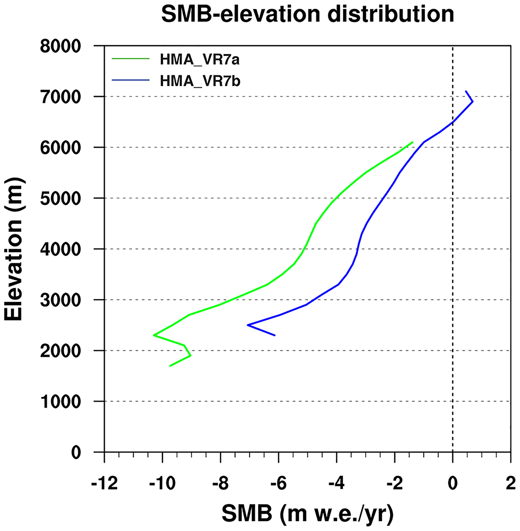
Figure 13Mean elevation profile of glacier SMB (m w.e. yr−1) over HMA for the period 1979–1998. The green and blue lines denote the SMB elevation profiles for HMA_VR7a and HMA_VR7b, respectively.
Table 4 shows the SMB components, which are integrated over the glacier area of the glacier cover datasets used in the respective HMA VR simulations. To enable comparison between the two simulations, the SMB components of HMA_VR7a have also been integrated over the glacier area of the updated dataset (marked as HMA_VR7a_GC2). The largest positive SMB term in both simulations is precipitation. CESM simulates the total annual precipitation of 111 ± 6 Gt yr−1 (90 ± 5 Gt yr−1) and 93 ± 4 Gt yr−1 in HMA_VR7a (HMA_VR7a_GC2) and HMA_VR7b, respectively. When integrated over the updated dataset, the total annual precipitation is higher in HMA_VR7b, likely because of increased snowfall and rainfall during spring in southern HMA (Fig. 8). For instance, in SE-HMA, the rainfall and snowfall increase from 131 mm per month in HMA_VR7a to 148 mm per month in HMA_VR7b, possibly because of the tuning of the cloud cover and the application of a newer microphysics scheme. The second-largest positive SMB term is refreezing, which increases from 29 ± 2 Gt yr−1 in HMA_V7a_GC2 to 32 ± 2 Gt yr−1 in HMA_VR7b. The increase in refreezing can mainly be attributed to the greater maximum snow depth.
Table 4Mean integrated SMB mass fluxes (Gt yr−1) for the period 1979–1998 in gigatons per year. The numbers in parentheses denote the standard deviation in time. The integrated SMB mass fluxes have been calculated over two different areas of integration for HMA_VR7a, as derived from the original and updated glacier cover datasets, respectively. The SMB mass fluxes for HMA_VR7a that are integrated over the glacier areas of the updated glacier cover dataset are denoted as HMA_VR7a_GC2. The mass fluxes of HMA_VR7b are only integrated over the glacier areas of the updated dataset.
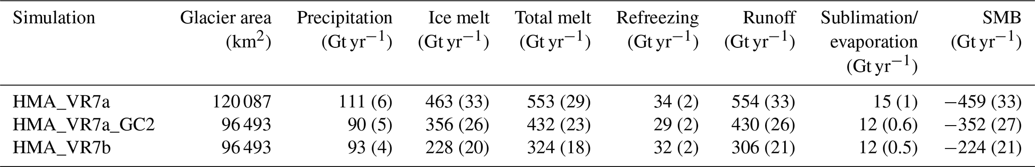
The largest SMB loss term in the HMA VR simulations is total melt, which is dominated by ice melt. The total (ice) melt volumes decrease from 432 ± 23 Gt yr−1 (356 ± 26 Gt yr−1) for HMA_VR7a_GC2 to 324 ± 18 Gt yr−1 (228 ± 20 Gt yr−1) for HMA_VR7b. The decreased melt can be attributed to several factors, including (1) a decrease in net radiation with increased cloud cover; (2) increased snowfall and higher maximum allowed snow depth, which increase refreezing capacity and snow persistence; (3) improved accuracy of glacier–elevation distribution with the updated glacier cover dataset; and (4) a higher albedo for bare ice. The latter increases the upwelling shortwave radiation. From Fig. 10 and Table 3, it is, however, not apparent that upwelling shortwave radiation increases between the two simulations because the SEB components in Fig. 10 and Table 3 are representative of the mean of all land units in glaciated grid cells. However, when selecting grid cells with a higher ice fraction (i.e., higher than 25 %), the upwelling shortwave radiation increases from 104 W m−2 for HMA_VR7a to 113 W m−2 for HMA_VR7b, as a result of a higher bare-ice albedo. The second-largest negative SMB term, sublimation and/or evaporation, is 12 Gt yr−1 for both simulations. Overall, the mass loss exceeds accumulation, giving a negative SMB. The integrated SMB is −352 ± 27 Gt yr−1 for HMA_VR7a_GC2 and −224 ± 21 Gt yr−1 for HMA_VR7b. The latter value is about 1.2 times higher than the Greenland ice sheet SMB (−182 ± 45 Gt yr−1) and 7 times higher than the Antarctic ice sheet SMB (−32 ± 4 Gt yr−1) for 2003–2016 (Lenaerts et al., 2019; the HMA ranges here represent 1 standard deviation, whereas Lenaerts et al., 2019, stated ranges with 2 standard deviations). Both values simulated on the HMA_VR7 grid are much more negative than the observed ranges of −13 ± 17 and −19 ± 2.5 Gt yr−1 for 1979–1998 and 2000–2015/2016, respectively (Brun et al., 2017; Shean et al., 2020; Zemp et al., 2019).
3.7 Future directions
Although many cryospheric–hydrological variables improve with increasing resolution, and VR-CESM can simulate positive SMB in parts of HMA, the negative SMB bias is cause for concern and suggests that model improvements are needed. There are several possible explanations for this bias. One explanation is the warm temperature bias over Central Asia, particularly over the Tibetan Plateau, as suggested in Sect. 3.1, 3.2, and 3.3. This warm bias could be related to underestimated cloud cover, which results in a higher net surface radiation due to increased downwelling solar radiation (partly offset by decreased downwelling longwave radiation, as suggested in Sect. 3.5). Improved convection and cloud parameterization schemes are needed. To make progress on the parameterization problem, we plan to carry out additional experiments nudging the upper vertical levels of CAM for variables such as horizontal wind, temperature, and humidity from ERA-Interim or ERA5, as previously done with WRF in HMA (de Kok et al., 2020). CAM contains flexible nudging capabilities (Wu et al., 2022; Kruse et al., 2022), with options for nudging over a particular region or level. The nudging tendencies, by definition, are co-located with the model bias, and an analysis of those tendencies constrains how the physics should interact with the dynamics at a particular grid resolution in order to provide a more realistic large-scale state (e.g., avoiding the anomalous large-scale subsidence in the free-running VR runs responsible for cloud biases on the northern side of the Tibetan Plateau). The nudging experiments also provide us with an opportunity to analyze the simulated surface mass balance, given a realistic atmospheric state, thereby helping to further isolate the cause of the deficiencies to the atmosphere or surface components.
Another reason for the negative SMB bias could be a lack of representation of surface processes in CLM that are important in complex mountain environments. For example, CLM neglects the role of aspect and orientation in the SEB (via solar illumination) and the glacier SMB. Wang et al. (2022) found out that 27.19 % of the HMA glaciers are subject to topographic shading, particularly for the north-facing glaciers of the Tibetan Plateau and the surrounding mountain ranges to the northwest and northeast (i.e., Kunlun Shan, Qilian Shan). Hillslope parameterization schemes (e.g., Swenson et al., 2019), which include the effects of aspect and orientation of a hillslope on the incoming solar radiation, could improve the simulation of SEB and SMB. Furthermore, CLM does not represent debris cover on mountain glaciers. About 12 %–13 % of the glaciers in HMA are at least partly covered by supraglacial debris, which, depending on its thickness, can accelerate or reduce glacial melt (by reducing surface albedo or insulating the surface, respectively; e.g., Herreid and Pellicciotti, 2020). Including debris cover in CLM surface datasets and adding debris-related glacial melt processes could be beneficial. Another weak point is the simulation of orographic precipitation in CLM. Currently, precipitation can be repartitioned as snow or rain, based on downscaled air temperature, but the effect of the topography on total precipitation is ignored, and the repartitioning applies fixed rain–snow temperature thresholds. Topography-based subgrid parameterizations such as the elevation-ratio-weighted method (ERWM; Tesfa et al., 2020) and more advanced rain–snow repartitioning schemes applying temperature–humidity–surface pressure-based rain–snow thresholds (Jennings et al., 2018) could improve the model's skill with respect to simulating high-altitude precipitation.
The negative SMB bias could also be related to the elevation class (EC) downscaling scheme in CLM and the way CLM and CAM are coupled. Figure 14 shows the relation between the grid cell mean SMB and glacier fraction (GCF) in 15 elevation zones at intervals of 250 m (based on the grid cell mean elevation). At lower elevations where glacier tongues reside, the glacier fraction is relatively low, whereas the most highly glaciated grid cells (with GCF higher than 90 %) have a mean grid cell elevation above 5000 m. In most elevation zones, SMB declines with decreasing glacier fraction. In some zones, such as 4000–4250 m, the SMB is more than 2 m w.e. yr−1 lower for sparsely glaciated cells (GCF of 0 %–10 %) than for highly glaciated cells (GCF of 90 %–100 %). In sparsely glaciated cells, elevation downscaling is only applied over glacier land units, whereas vegetated land units are excluded from downscaling. Moreover, the coupling between CLM and CAM is based on the homogenized state of a CLM grid cell (i.e., the average over all land units within the grid cell). This means that in grid cells with small ice fractions, the impact of glaciers is limited, and the mean depends mainly on fluxes from vegetated land units. CAM receives this homogenized state and subsequently couples back to CLM, with the downscaling of a few atmospheric variables, such as near-surface temperature. If the glacier patch lies higher than the grid cell mean elevation (and thus the elevation of the vegetated land unit), then the glacier land unit sees a cooler air temperature than the vegetated land unit. However, the atmospheric temperature coupled to CLM could be dominated by the lower-lying and warmer vegetated land unit. This could result in warmer glacier temperatures that make the SMB more negative. One potential solution is to apply elevation downscaling over all land units using the hillslope model of Swenson et al. (2019). Another is to improve the subgrid coupling between CLM and CAM by introducing CLM patch information into CAM; this is the focus of the CLASP (Coupling of Land and Atmosphere Subgrid Parameterizations) project (Waterman et al., 2022). The necessity for the improvement of land–atmosphere coupling (via elevation downscaling) is also suggested by offline 3-year (1979–1981) CLM simulations performed on the HMA_VR7 grid and driven by observation- and reanalysis-based meteorological forcings of the Global Soil Wetness Project Phase 3 (GSWP3; Dirmeyer et al., 2006), which is a default offline mode in CLM. The offline CLM simulations (referred to as HMALOa and HMALOb; i.e., following the HMA_VR7a and HMA_VR7b settings, respectively) likewise show a declining SMB with a decreasing glacier fraction (Fig. S3), which suggests that the improvement of land–atmosphere coupling is crucial. The offline CLM simulations nonetheless show that the colder and wetter surface climate in the HMA VR simulations help to reduce the SMB bias (Figs. S4 and S5; Table S3).
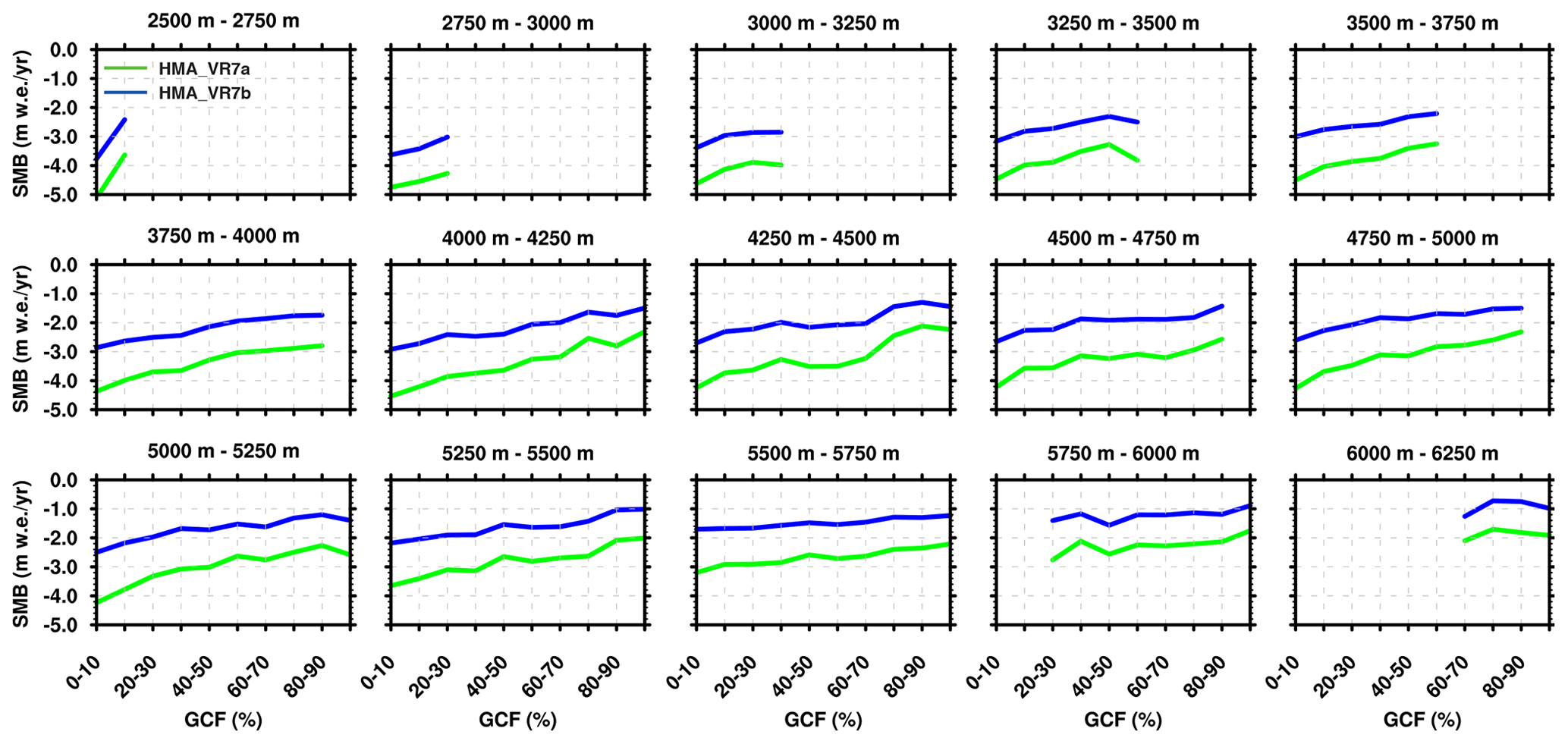
Figure 14CLM grid cell mean SMB glacier fraction distributions for HMA_VR7a (green) and HMA_VR7b (blue). The SMB glacier elevation distributions are calculated for 15 different 250 m elevation zones between 2500 and 6250 m altitude, where the elevation zones are based on CLM grid cell mean elevation distributions.
In this study, the spectral element dynamical core used by CESM is based on the hydrostatic approximation, which means non-hydrostatic vertical acceleration terms are neglected. Although we believe that there are insufficient grounds to deem our model configuration inappropriate, we are aware that the hydrostatic version in combination with a 7 km regionally refined grid could propagate model-related uncertainties into the modeled outputs, such as precipitation, wind, and cloud cover, which eventually could also affect the SEB and SMB. To address these model-related uncertainties, one potential solution could be to apply a similar regionally refined grid in combination with the newly developed MPAS (Model for Prediction Across Scales) non-hydrostatic dynamical core, which has recently successfully been applied over the western USA mountain ranges (Huang et al., 2022).
Finally, the version of CAM used in this study has 32 levels in the vertical, which was developed for the standard 1∘ configuration in CESM2 and is a typical vertical resolution used for low-top (∼ 40 km) CMIP6 class models. This coarser vertical grid may not be appropriate when increasing the horizontal resolution beyond 1∘ (Skamarock et al., 2019; Lindzen and Fox-Rabinovitz, 1989), such as our HMA_VR7 configuration, but has nonetheless shown to improve the model fidelity regardless (Gettelman et al., 2018; Herrington and Reed, 2020; Herrington et al., 2022; van Kampenhout et al., 2019; Rhoades et al., 2018), as also shown in our study here. A new 58-level, low-top vertical grid slated for the CESM3 model may be preferable to reduce the noise and spurious flow features.
We have investigated the ability of the variable-resolution Community Earth System Model to simulate cryospheric–hydrological variables such as glacier surface mass balance and snow conditions over High Mountain Asia. To this end, we developed a new VR grid with regional refinement up to 7 km over HMA. With this grid, we ran two 20-year (1979–1998) model simulations. The second model simulation includes an updated glacier cover dataset and several atmosphere and land model modifications. We evaluated the results by comparing them to the gridded outputs derived from a globally uniform 1∘ CESM grid, reanalysis-, satellite-, and observation-based datasets, and a WRF-based glacier model.
The evaluations show that the large-scale circulation on the HMA_VR7 grid generally compares well with ERA5 but has an upper-troposphere warm temperature bias at midlatitudes during summer. This warm bias grows with increasing horizontal resolution (+2 K for NE30 and +3 K for HMA_VR7). Furthermore, the HMA VR runs have less cloud cover than NE30 runs, which is likely related to enhanced subsidence driven by more intense monsoonal circulation and to the shorter physics time step in the HMA runs. The HMA VR runs also have a summertime warm temperature bias (up to about +2.5 ∘C) at the surface, but this bias is smaller than for NE30, likely because of elevation downscaling. Most HMA subregions have cold temperature biases during winter and to lesser extent during other seasons; these biases grow with increasing resolution. Overall, the HMA VR runs simulate rainfall, snowfall, snow cover, and snow depth better than NE30 but with some biases. Rainfall biases occur mainly in monsoon-dominated regions, whereas snowfall, snow cover, and snow depth biases are largest during winter and spring in southwestern HMA, in part because of the cold temperature bias and the HMA_VR7b model modifications. Snow cover is underestimated during summer but agrees better than NE30 with NSIDC snow cover.
The HMA VR runs have more downwelling shortwave radiation and less downwelling longwave radiation compared to NE30, JRA-55, and CERES-EBAF. This can be attributed to negative cloud cover biases that reduce longwave absorption and lower the albedo. The HMA VR runs have greater net radiation at the surface, resulting in higher melting and a positive (upward) conductive heat flux. The high volumes of snow and ice melting translate into an SMB that is more negative than observation-based glaciological and geodetic mass balances and WRF-based results. The HMA_VR7b simulation has a smaller SMB bias than HMA_VR7a, with an integrated SMB over glaciers of −224 ± 21 Gt yr−1, compared to −352 ± 28 Gt yr−1 for HMA_VR7a.
This study shows that VR-CESM generally reduces climatological biases relative to a coarse-resolution CESM grid and could be a useful tool for simulating cryospheric–hydrological variables, such as glacier SMB, in HMA. However, improvements are still needed to reduce cloud cover and temperature biases, improve the model physics and land–atmosphere coupling, and, thereby, simulate SMB more accurately. This study could be a starting point for simulating cryospheric–hydrological variables in HMA and other mountain glacier regions with VR-CESM and other GCMs and ESMs.
Publicly available data are stored in two separate data archives on Zenodo. The first archive (https://doi.org/10.5281/zenodo.7864689, Wijngaard et al., 2023a) contains the model scripts and files that were used to create the updated glacier cover dataset. The second archive (https://doi.org/10.5281/zenodo.7864633, Wijngaard et al., 2023b) contains the NE30 and HMA_VR7 grid variables that were used to generate most of the figures in this work. The remainder of the data are available on request to the corresponding authors.
The supplement related to this article is available online at: https://doi.org/10.5194/tc-17-3803-2023-supplement.
RRW, ARH, WHL, and GRL designed the study. RRW and ARH modified the model code as needed. RRW ran the model. RRW and ARH analyzed the model results and prepared the text and figures. SIA supervised RRW. All authors contributed to the final text.
The contact author has declared that none of the authors has any competing interests.
Publisher's note: Copernicus Publications remains neutral with regard to jurisdictional claims in published maps and institutional affiliations.
We would like to thank the editor and reviewers for their constructive remarks and suggestions that helped us to improve the paper significantly. We greatly acknowledge Samar Minallah, Leo van Kampenhout, Bill Sacks, Julio Bacmeister, and Peter Hjort Lauritzen for the helpful discussions and support. This work has been supported by the National Research Foundation of Korea (NRF) grant funded by the Korea government (MSIT; grant no. NRF-2018R1A5A1024958). Adam R. Herrington, William H. Lipscomb, and Gunter R. Leguy have been supported by the National Center for Atmospheric Research, which is a major facility sponsored by the National Science Foundation (grant no. 1852977). Computing and data storage resources, including the Cheyenne supercomputer (https://doi.org/10.5065/D6RX99HX, Computational and Information Systems Laboratory, 2019), were provided by the Computational and Information Systems Laboratory (CISL) at NCAR.
This research has been supported by the National Research Foundation of Korea (grant no. NRF-2018R1A5A1024958) and the National Center for Atmospheric Research (grant no. 1852977).
This paper was edited by Emily Collier and reviewed by two anonymous referees.
Bambach, N. E., Rhoades, A. M., Hatchett, B. J., Jones, A. D., Ullrich, P. A., and Zarzycki, C. M.: Projecting climate change in South America using variable-resolution Community Earth System Model: An application to Chile, Int. J. Climatol., 42, 2514–2542, https://doi.org/10.1002/joc.7379, 2021.
Beljaars, A. C. M., Brown, A. R., and Wood, N.: A new parametrization of turbulent orographic form drag, Q. J. Roy. Meteor. Soc., 130, 1327–1347, https://doi.org/10.1256/qj.03.73, 2004.
Bogenschutz, P. A., Gettelman, A., Morrison, H., Larson, V. E., Craig, C., and Schanen, D. P.: Higher-order turbulence closure and its impact on climate simulations in the community atmosphere model, J. Climate, 26, 9655–9676, https://doi.org/10.1175/JCLI-D-13-00075.1, 2013.
Bonekamp, P. N. J., de Kok, R. J., Collier, E., and Immerzeel, W. W.: Contrasting Meteorological Drivers of the Glacier Mass Balance Between the Karakoram and Central Himalaya, Front. Earth Sci., 7, 107, https://doi.org/10.3389/feart.2019.00107, 2019.
Brodzik, M. J. and Armstrong, R.: Northern Hemisphere EASE-Grid 2.0 Weekly Snow Cover and Sea Ice Extent, Version 4, Boulder, Colorado USA, NASA DAAC at the National Snow and Ice Data Center [data set], https://doi.org/10.5067/P7O0HGJLYUQU, 2013.
Brun, F., Berthier, E., Wagnon, P., Kääb, A., and Treichler, D.: A spatially resolved estimate of High Mountain Asia glacier mass balances from 2000 to 2016, Nat. Geosci., 10, 668–673, https://doi.org/10.1038/ngeo2999, 2017.
Cannon, F., Carvalho, L. M. V., Jones, C., and Bookhagen, B.: Multi-annual variations in winter westerly disturbance activity affecting the Himalaya, Clim. Dynam., 44, 441–455, https://doi.org/10.1007/s00382-014-2248-8, 2015.
Collier, E., Mölg, T., Maussion, F., Scherer, D., Mayer, C., and Bush, A. B. G.: High-resolution interactive modelling of the mountain glacier–atmosphere interface: an application over the Karakoram, The Cryosphere, 7, 779–795, https://doi.org/10.5194/tc-7-779-2013, 2013.
Computational and Information Systems Laboratory: Cheyenne supercomputer, https://doi.org/10.5065/D6RX99HX, 2019.
Danabasoglu, G., Lamarque, J. F., Bacmeister, J., Bailey, D. A., DuVivier, A. K., Edwards, J., Emmons, L. K., Fasullo, J., Garcia, R., Gettelman, A., Hannay, C., Holland, M. M., Large, W. G., Lauritzen, P. H., Lawrence, D. M., Lenaerts, J. T. M., Lindsay, K., Lipscomb, W. H., Mills, M. J., Neale, R., Oleson, K. W., Otto-Bliesner, B., Phillips, A. S., Sacks, W., Tilmes, S., van Kampenhout, L., Vertenstein, M., Bertini, A., Dennis, J., Deser, C., Fischer, C., Fox-Kemper, B., Kay, J. E., Kinnison, D., Kushner, P. J., Larson, V. E., Long, M. C., Mickelson, S., Moore, J. K., Nienhouse, E., Polvani, L., Rasch, P. J., and Strand, W. G.: The Community Earth System Model Version 2 (CESM2), J. Adv. Model Earth. Sy., 12, e2019MS001916, https://doi.org/10.1029/2019MS001916, 2020.
Danielson, J. J. and Gesch, D. B.: Global Multi-resolution Terrain Elevation Data 2010 (GMTED2010), U.S. Geological Survey Open-File Report 2011-1073, 2011.
de Kok, R. J., Kraaijenbrink, P. D. A., Tuinenburg, O. A., Bonekamp, P. N. J., and Immerzeel, W. W.: Towards understanding the pattern of glacier mass balances in High Mountain Asia using regional climatic modelling, The Cryosphere, 14, 3215–3234, https://doi.org/10.5194/tc-14-3215-2020, 2020.
Dirmeyer, P. A., Gao, X., Zhao, M., Guo, Z., Oki, T., and Hanasaki, N.: GSWP-2: Multimodel analysis and implications for our perception of the land surface, B. Am. Meteorol. Soc., 87, 1381–1398, https://doi.org/10.1175/BAMS-87-10-1381, 2006.
Dudhia, J.: A nonhydrostatic version of the Penn State-NCAR mesoscale model: validation tests and simulation of an Atlantic cyclone and cold front, Mon. Weather Rev., 121, 1493–1513, https://doi.org/10.1175/1520-0493(1993)121<1493:ANVOTP>2.0.CO;2, 1993.
Dudhia, J.: A history of mesoscale model development, Asia Pac. J. Atmos. Sci., 50, 121–131, https://doi.org/10.1007/s13143-014-0031-8, 2014.
Flanner, M. G. and Zender, C. S.: Snowpack radiative heating: Influence on Tibetan Plateau climate, Geophys. Res. Lett., 32, L06501, https://doi.org/10.1029/2004GL022076, 2005.
Flanner, M. G., Zender, C. S., Randerson, J. T., and Rasch, P. J.: Present-day climate forcing and response from black carbon in snow, J. Geophys. Res.-Atmos., 112, D11202, https://doi.org/10.1029/2006JD008003, 2007.
Frey, H., Haeberli, W., Linsbauer, A., Huggel, C., and Paul, F.: A multi-level strategy for anticipating future glacier lake formation and associated hazard potentials, Nat. Hazards Earth Syst. Sci., 10, 339–352, https://doi.org/10.5194/nhess-10-339-2010, 2010.
Gates, W. L., Boyle, J. S., Covey, C., Dease, C. G., Doutriaux, C. M., Drach, R. S., Fiorino, M., Gleckler, P. J., Hnilo, J. J., Marlais, S. M., Phillips, T. J., Potter, G. L., Santer, B. D., Sperber, K. R., Taylor, K. E., and Williams, D. N.: An Overview of the Results of the Atmospheric Model Intercomparison Project (AMIP I), B. Am. Meteorol. Soc., 80, 29–55, https://doi.org/10.1175/1520-0477(1999)080<0029:AOOTRO>2.0.CO;2, 1999.
Gettelman, A. and Morrison, H.: Advanced two-moment bulk microphysics for global models. Part I: Off-line tests and comparison with other schemes, J. Climate, 28, 1268–1287, https://doi.org/10.1175/JCLI-D-14-00102.1, 2015.
Gettelman, A., Callaghan, P., Larson, V. E., Zarzycki, C. M., Bacmeister, J. T., Lauritzen, P. H., Bogenschutz, P. A., and Neale, R. B.: Regional Climate Simulations With the Community Earth System Model, J. Adv. Model Earth Sy., 46, 8329–8337, https://doi.org/10.1002/2017MS001227, 2018.
Gettelman, A., Hannay, C., Bacmeister, J. T., Neale, R. B., Pendergrass, A. G., Danabasoglu, G., Lamarque, J. F., Fasullo, J. T., Bailey, D. A., Lawrence, D. M., and Mills, M. J.: High Climate Sensitivity in the Community Earth System Model Version 2 (CESM2), Geophys. Res. Lett., 46, https://doi.org/10.1029/2019GL083978, 2019a.
Gettelman, A., Morrison, H., Thayer-Calder, K., and Zarzycki, C. M.: The Impact of Rimed Ice Hydrometeors on Global and Regional Climate, J. Adv. Model Earth Sy., 11, 1543–1562, https://doi.org/10.1029/2018MS001488, 2019b.
Gu, H., Wang, G., Yu, Z., and Mei, R.: Assessing future climate changes and extreme indicators in east and south Asia using the RegCM4 regional climate model, Climatic Change, 114, 301–317, https://doi.org/10.1007/s10584-012-0411-y, 2012.
Guba, O., Taylor, M. A., Ullrich, P. A., Overfelt, J. R., and Levy, M. N.: The spectral element method (SEM) on variable-resolution grids: evaluating grid sensitivity and resolution-aware numerical viscosity, Geosci. Model Dev., 7, 2803–2816, https://doi.org/10.5194/gmd-7-2803-2014, 2014.
Herreid, S. and Pellicciotti, F.: The state of rock debris covering Earth's glaciers, Nat. Geosci., 13, 621–627, https://doi.org/10.1038/s41561-020-0615-0, 2020.
Herrington, A. R. and Reed, K. A.: On resolution sensitivity in the Community Atmosphere Model, Q. J. Roy. Meteor. Soc., 146, 3789–3807, https://doi.org/10.1002/qj.3873, 2020.
Herrington, A. R., Lauritzen, P. H., Lofverstrom, M., Lipscomb, W. H., Gettelman, A., and Taylor, M. A.: Impact of grids and dynamical cores in CESM2.2 on the surface mass balance of the Greenland Ice Sheet, J. Adv. Model Earth Sy., 14, e2022MS003192, https://doi.org/10.1029/2022MS003192, 2022.
Hersbach, H., Bell, B., Berrisford, P., Hirahara, S., Horányi, A., Muñoz-Sabater, J., Nicolas, J., Peubey, C., Radu, R., Schepers, D., Simmons, A., Soci, C., Abdalla, S., Abellan, X., Balsamo, G., Bechtold, P., Biavati, G., Bidlot, J., Bonavita, M., De Chiara, G., Dahlgren, P., Dee, D., Diamantakis, M., Dragani, R., Flemming, J., Forbes, R., Fuentes, M., Geer, A., Haimberger, L., Healy, S., Hogan, R. J., Hólm, E., Janisková, M., Keeley, S., Laloyaux, P., Lopez, P., Lupu, C., Radnoti, G., de Rosnay, P., Rozum, I., Vamborg, F., Villaume, S., and Thépaut, J. N.: The ERA5 global reanalysis, Q. J. Roy. Meteor. Soc., 146, 1999–2049, https://doi.org/10.1002/qj.3803, 2020.
Hock, R., Rasul, G., Adler, C., Cáceres, B., Gruber, S., Hirabayashi, Y., Jackson, M., Kääb, A., Kang, S., Kutuzov, S., Milner, A., Molau, U., Morin, S., Orlove, B., and Steltzer, H. I.: High Mountain Areas, in: IPCC Special Report on the Ocean and Cryosphere in a Changing Climate, edited by: Pörtner, H.-O., Roberts, D. C., Masson-Delmotte, V., Zhai, P., Tignor, M., Poloczanska, E., Mintenbeck, K., Alegriìa, A., Nicolai, M., Okem, A., Petzold, J., Rama, B., and Weyer, N. M., IPCC Intergovernmental Panel on Climate Change, Geneva, Switzerland, Cambridge University Press, Cambridge, UK and New York, NY, USA, 131–202, https://doi.org/10.1017/9781009157964.004, 2019.
Huang, X., Rhoades, A. M., Ullrich, P. A., and Zarzycki, C. M.: An evaluation of the variable-resolution CESM for modeling California's climate, J. Adv. Model Earth Sy., 8, 345–369, https://doi.org/10.1002/2015MS000559, 2016.
Huang, X., Gettelman, A., Skamarock, W. C., Lauritzen, P. H., Curry, M., Herrington, A., Truesdale, J. T., and Duda, M.: Advancing precipitation prediction using a new-generation storm-resolving model framework – SIMA-MPAS (V1.0): a case study over the western United States, Geosci. Model Dev., 15, 8135–8151, https://doi.org/10.5194/gmd-15-8135-2022, 2022.
Hurrell, J. W., Hack, J. J., Shea, D., Caron, J. M., and Rosinski, J.: A new sea surface temperature and sea ice boundary dataset for the community atmosphere model, J. Climate, 21, 5145–5153, https://doi.org/10.1175/2008JCLI2292.1, 2008.
Hurtt, G. C., Chini, L., Sahajpal, R., Frolking, S., Bodirsky, B. L., Calvin, K., Doelman, J. C., Fisk, J., Fujimori, S., Klein Goldewijk, K., Hasegawa, T., Havlik, P., Heinimann, A., Humpenöder, F., Jungclaus, J., Kaplan, J. O., Kennedy, J., Krisztin, T., Lawrence, D., Lawrence, P., Ma, L., Mertz, O., Pongratz, J., Popp, A., Poulter, B., Riahi, K., Shevliakova, E., Stehfest, E., Thornton, P., Tubiello, F. N., van Vuuren, D. P., and Zhang, X.: Harmonization of global land use change and management for the period 850–2100 (LUH2) for CMIP6, Geosci. Model Dev., 13, 5425–5464, https://doi.org/10.5194/gmd-13-5425-2020, 2020.
Immerzeel, W. W., Wanders, N., Lutz, A. F., Shea, J. M., and Bierkens, M. F. P.: Reconciling high-altitude precipitation in the upper Indus basin with glacier mass balances and runoff, Hydrol. Earth Syst. Sci., 19, 4673–4687, https://doi.org/10.5194/hess-19-4673-2015, 2015.
Immerzeel, W. W., Lutz, A. F., Andrade, M., Bahl, A., Biemans, H., Bolch, T., Hyde, S., Brumby, S., Davies, B. J., Elmore, A. C., Emmer, A., Feng, M., Fernández, A., Haritashya, U., Kargel, J. S., Koppes, M., Kraaijenbrink, P. D. A., Kulkarni, A. v., Mayewski, P. A., Nepal, S., Pacheco, P., Painter, T. H., Pellicciotti, F., Rajaram, H., Rupper, S., Sinisalo, A., Shrestha, A. B., Viviroli, D., Wada, Y., Xiao, C., Yao, T., and Baillie, J. E. M.: Importance and vulnerability of the world's water towers, Nature, 577, 364–369, https://doi.org/10.1038/s41586-019-1822-y, 2020.
Jang, J. and Hong, S. Y.: Comparison of simulated precipitation over East Asia in two regional models with hydrostatic and nonhydrostatic dynamical cores, Mon. Weather Rev., 144, 3579–3590, https://doi.org/10.1175/MWR-D-15-0428.1, 2016.
Janjic, Z. I., Gerrity, J., and Nickovic, S.: An alternative approach to nonhydrostatic modeling, Mon. Weather Rev., 129, 1164–1178, https://doi.org/10.1175/1520-0493(2001)129<1164:AAATNM>2.0.CO;2, 2001.
Jeevanjee, N.: Vertical Velocity in the Gray Zone, J. Adv. Model Earth Sy., 9, 2304–2316, https://doi.org/10.1002/2017MS001059, 2017.
Jennings, K. S., Winchell, T. S., Livneh, B., and Molotch, N. P.: Spatial variation of the rain-snow temperature threshold across the Northern Hemisphere, Nat. Commun., 9, 1148, https://doi.org/10.1038/s41467-018-03629-7, 2018.
Jiang, X., Wu, C., Chen, B., Wang, W., Liu, X., Lin, Z., and Han, Z.: Exploring a variable-resolution approach for simulating the regional climate in Southwest China using VR-CESM, Atmos. Res., 292, 106851, https://doi.org/10.1016/j.atmosres.2023.106851, 2023.
Kato, S., Rose, F. G., Rutan, D. A., Thorsen, T. J., Loeb, N. G., Doelling, D. R., Huang, X., Smith, W. L., Su, W., and Ham, S. H.: Surface irradiances of edition 4.0 Clouds and the Earth's Radiant Energy System (CERES) Energy Balanced and Filled (EBAF) data product, J. Climate, 31, 4501–4527, https://doi.org/10.1175/JCLI-D-17-0523.1, 2018.
Kato, T.: Hydrostatic and non-hydrostatic simulations of the 6 August 1993 Kagoshima torrential rain, J. Meteorol. Soc. Jpn., 74, 355–363, https://doi.org/10.2151/jmsj1965.74.3_355, 1996.
Klein Goldewijk, K., Beusen, A., Doelman, J., and Stehfest, E.: Anthropogenic land use estimates for the Holocene – HYDE 3.2, Earth Syst. Sci. Data, 9, 927–953, https://doi.org/10.5194/essd-9-927-2017, 2017.
Kobayashi, S., Ota, Y., Harada, Y., Ebita, A., Moriya, M., Onoda, H., Onogi, K., Kamahori, H., Kobayashi, C., Endo, H., Miyaoka, K., and Kiyotoshi, T.: The JRA-55 reanalysis: General specifications and basic characteristics, J. Meteorol. Soc. Jpn., 93, 5–48, https://doi.org/10.2151/jmsj.2015-001, 2015.
Körner, C., Jetz, W., Paulsen, J., Payne, D., Rudmann-Maurer, K., and M. Spehn, E.: A global inventory of mountains for bio-geographical applications, Alp. Bot., 127, 1–15, https://doi.org/10.1007/s00035-016-0182-6, 2017.
Kraaijenbrink, P. D. A., Bierkens, M. F. P., Lutz, A. F., and Immerzeel, W. W.: Impact of a global temperature rise of 1.5 degrees Celsius on Asia's glaciers, Nature, 549, 257–260, https://doi.org/10.1038/nature23878, 2017.
Kruse, C. G., Bacmeister, J. T., Zarzycki, C. M., Larson, V. E., and Thayer-Calder, K.: Do Nudging Tendencies Depend on the Nudging Timescale Chosen in Atmospheric Models?, J. Adv. Model Earth Sy., 14, e2022MS003024, https://doi.org/10.1029/2022MS003024, 2022.
Lalande, M., Ménégoz, M., Krinner, G., Naegeli, K., and Wunderle, S.: Climate change in the High Mountain Asia in CMIP6, Earth Syst. Dynam., 12, 1061–1098, https://doi.org/10.5194/esd-12-1061-2021, 2021.
Lauritzen, P. H., Bacmeister, J. T., Callaghan, P. F., and Taylor, M. A.: NCAR_Topo (v1.0): NCAR global model topography generation software for unstructured grids, Geosci. Model Dev., 8, 3975–3986, https://doi.org/10.5194/gmd-8-3975-2015, 2015.
Lauritzen, P. H., Nair, R. D., Herrington, A. R., Callaghan, P., Goldhaber, S., Dennis, J. M., Bacmeister, J. T., Eaton, B. E., Zarzycki, C. M., Taylor, M. A., Ullrich, P. A., Dubos, T., Gettelman, A., Neale, R. B., Dobbins, B., Reed, K. A., Hannay, C., Medeiros, B., Benedict, J. J., and Tribbia, J. J.: NCAR Release of CAM-SE in CESM2.0: A Reformulation of the Spectral Element Dynamical Core in Dry-Mass Vertical Coordinates With Comprehensive Treatment of Condensates and Energy, J. Adv. Model Earth Sy., 10, 1537–1570, https://doi.org/10.1029/2017MS001257, 2018.
Lawrence, D. M., Fisher, R. A., Koven, C. D., Oleson, K. W., Swenson, S. C., Bonan, G., Collier, N., Ghimire, B., Kampenhout, L., Kennedy, D., Kluzek, E., Lawrence, P. J., Li, F., Li, H., Lombardozzi, D., Riley, W. J., Sacks, W. J., Shi, M., Vertenstein, M., Wieder, W. R., Xu, C., Ali, A. A., Badger, A. M., Bisht, G., Broeke, M., Brunke, M. A., Burns, S. P., Buzan, J., Clark, M., Craig, A., Dahlin, K., Drewniak, B., Fisher, J. B., Flanner, M., Fox, A. M., Gentine, P., Hoffman, F., Keppel-Aleks, G., Knox, R., Kumar, S., Lenaerts, J., Leung, L. R., Lipscomb, W. H., Lu, Y., Pandey, A., Pelletier, J. D., Perket, J., Randerson, J. T., Ricciuto, D. M., Sanderson, B. M., Slater, A., Subin, Z. M., Tang, J., Thomas, R. Q., Val Martin, M., and Zeng, X.: The Community Land Model Version 5: Description of New Features, Benchmarking, and Impact of Forcing Uncertainty, J. Adv. Model Earth Sy., 11, 4245–4287, https://doi.org/10.1029/2018MS001583, 2019.
Lenaerts, J. T. M., Vizcaino, M., Fyke, J., van Kampenhout, L., and van den Broeke, M. R.: Present-day and future Antarctic ice sheet climate and surface mass balance in the Community Earth System Model, Clim. Dynam., 47, 1367–1381, https://doi.org/10.1007/s00382-015-2907-4, 2016.
Lenaerts, J. T. M., Medley, B., van den Broeke, M. R., and Wouters, B.: Observing and Modeling Ice Sheet Surface Mass Balance, Rev. Geophys., 57, 376–420, https://doi.org/10.1029/2018RG000622, 2019.
Li, D., Lu, X., Walling, D. E., Zhang, T., Steiner, J. F., Wasson, R. J., Harrison, S., Nepal, S., Nie, Y., Immerzeel, W. W., Shugar, D. H., Koppes, M., Lane, S., Zeng, Z., Sun, X., Yegorov, A., and Bolch, T.: High Mountain Asia hydropower systems threatened by climate-driven landscape instability, Nat. Geosci., 15, 520–530, https://doi.org/10.1038/s41561-022-00953-y, 2022.
Lindzen, R. S. and Fox-Rabinovitz, M.: Consistent vertical and horizontal resolution, Mon. Weather Rev., 117, 2575–2583, https://doi.org/10.1175/1520-0493(1989)117<2575:CVAHR>2.0.CO;2, 1989.
Lipscomb, W. H., Fyke, J. G., Vizcaíno, M., Sacks, W. J., Wolfe, J., Vertenstein, M., Craig, A., Kluzek, E., and Lawrence, D. M.: Implementation and Initial Evaluation of the Glimmer Community Ice Sheet Model in the Community Earth System Model, J. Climate, 26, 7352–7371, https://doi.org/10.1175/JCLI-D-12-00557.1, 2013.
Lipscomb, W. H., Price, S. F., Hoffman, M. J., Leguy, G. R., Bennett, A. R., Bradley, S. L., Evans, K. J., Fyke, J. G., Kennedy, J. H., Perego, M., Ranken, D. M., Sacks, W. J., Salinger, A. G., Vargo, L. J., and Worley, P. H.: Description and evaluation of the Community Ice Sheet Model (CISM) v2.1, Geosci. Model Dev., 12, 387–424, https://doi.org/10.5194/gmd-12-387-2019, 2019.
Liu, W., Ullrich, P. A., Guba, O., Caldwell, P. M., and Keen, N. D.: An Assessment of Nonhydrostatic and Hydrostatic Dynamical Cores at Seasonal Time Scales in the Energy Exascale Earth System Model (E3SM), J. Adv. Model Earth. Sy., 14, e2021MS002805, https://doi.org/10.1029/2021MS002805, 2022.
Liu, X., Ma, P.-L., Wang, H., Tilmes, S., Singh, B., Easter, R. C., Ghan, S. J., and Rasch, P. J.: Description and evaluation of a new four-mode version of the Modal Aerosol Module (MAM4) within version 5.3 of the Community Atmosphere Model, Geosci. Model Dev., 9, 505–522, https://doi.org/10.5194/gmd-9-505-2016, 2016.
Loeb, N. G., Doelling, D. R., Wang, H., Su, W., Nguyen, C., Corbett, J. G., Liang, L., Mitrescu, C., Rose, F. G., and Kato, S.: Clouds and the Earth'S Radiant Energy System (CERES) Energy Balanced and Filled (EBAF) top-of-atmosphere (TOA) edition-4.0 data product, J. Climate, 31, 895–918, https://doi.org/10.1175/JCLI-D-17-0208.1, 2018.
Lutz, A. F., ter Maat, H. W., Wijngaard, R. R., Biemans, H., Syed, A., Shrestha, A. B., Wester, P., and Immerzeel, W. W.: South Asian river basins in a 1.5 ∘C warmer world, Reg. Environ. Change, 19, 833–847, https://doi.org/10.1007/s10113-018-1433-4, 2019.
Lutz, A. F., Immerzeel, W. W., Siderius, C., Wijngaard, R. R., Nepal, S., Shrestha, A. B., Wester, P., and Biemans, H.: South Asian agriculture increasingly dependent on meltwater and groundwater, Nat. Clim. Change, 12, 566–573, https://doi.org/10.1038/s41558-022-01355-z, 2022.
Marzeion, B., Hock, R., Anderson, B., Bliss, A., Champollion, N., Fujita, K., Huss, M., Immerzeel, W. W., Kraaijenbrink, P., Malles, J., Maussion, F., Radić, V., Rounce, D. R., Sakai, A., Shannon, S., Wal, R., and Zekollari, H.: Partitioning the Uncertainty of Ensemble Projections of Global Glacier Mass Change, Earths Future, 8, e2019EF001470, https://doi.org/10.1029/2019EF001470, 2020.
Mölg, T. and Kaser, G.: A new approach to resolving climate-cryosphere relations: Downscaling climate dynamics to glacier-scale mass and energy balance without statistical scale linking, J. Geophys. Res., 116, D16101, https://doi.org/10.1029/2011JD015669, 2011.
Muntjewerf, L., Sacks, W. J., Lofverstrom, M., Fyke, J., Lipscomb, W. H., Ernani da Silva, C., Vizcaino, M., Thayer-Calder, K., Lenaerts, J. T. M., and Sellevold, R.: Description and Demonstration of the Coupled Community Earth System Model v2 – Community Ice Sheet Model v2 (CESM2-CISM2), J. Adv. Model Earth Sy., 13, e2020MS002356, https://doi.org/10.1029/2020MS002356, 2021.
Nie, Y., Pritchard, H. D., Liu, Q., Hennig, T., Wang, W., Wang, X., Liu, S., Nepal, S., Samyn, D., Hewitt, K., and Chen, X.: Glacial change and hydrological implications in the Himalaya and Karakoram, Nat. Rev. Earth Environ., 2, 91–106, https://doi.org/10.1038/s43017-020-00124-w, 2021.
Oleson, K. W., Lawrence, D. M., Bonan, G. B., Drewniak, B., Huang, M., Koven, C. D. , Levis, S., Li, F., Riley, W. J., Subin, Z. M., Swenson, S., Thornton, P. E. , Bozbiyik, A., Fisher, R., Heald, C. L., Kluzek, E., Lamarque, J.-F., Ruby Leung, L., Lipscomb, W., Muszala, S. P., Ricciuto, D. M., Sacks, W. J., Tang, J., and Yang, Z.-L.: Technical description of version 4.5 of the Community Land Model (CLM), Ncar Tech. Note NCAR/TN-503+STR. National Center for Atmospheric Research, Boulder, 1–434, https://doi.org/10.5065/D6RR1W7M, 2013.
Orsolini, Y., Wegmann, M., Dutra, E., Liu, B., Balsamo, G., Yang, K., de Rosnay, P., Zhu, C., Wang, W., Senan, R., and Arduini, G.: Evaluation of snow depth and snow cover over the Tibetan Plateau in global reanalyses using in situ and satellite remote sensing observations, The Cryosphere, 13, 2221–2239, https://doi.org/10.5194/tc-13-2221-2019, 2019.
Palazzi, E., Von Hardenberg, J., Terzago, S., and Provenzale, A.: Precipitation in the Karakoram-Himalaya: a CMIP5 view, Clim. Dynam., 45, 21–45, https://doi.org/10.1007/s00382-014-2341-z, 2015.
Rahimi, S. R., Wu, C., Liu, X., and Brown, H.: Exploring a Variable-Resolution Approach for Simulating Regional Climate Over the Tibetan Plateau Using VR-CESM, J. Geophys. Res.-Atmos., 124, 4490–4513, https://doi.org/10.1029/2018JD028925, 2019.
Rauscher, S. A., Ringler, T. D., Skamarock, W. C., and Mirin, A. A.: Exploring a global multiresolution modeling approach using aquaplanet simulations, J. Climate, 26, 2432–2452, https://doi.org/10.1175/JCLI-D-12-00154.1, 2013.
RGI-Consortium: Randolph Glacier Inventory – A Dataset of Global Glacier Outlines: Version 6.0, Technical Report, Global Land Ice Measurements from Space, Colorado, USA, Boulder, Colorado, USA, https://doi.org/10.7265/4m1f-gd79, 2017.
Rhoades, A. M., Huang, X., Ullrich, P. A., and Zarzycki, C. M.: Characterizing Sierra Nevada Snowpack Using Variable-Resolution CESM, J. Appl. Meteorol. Clim., 55, 173–196, https://doi.org/10.1175/JAMC-D-15-0156.1, 2016.
Rhoades, A. M., Ullrich, P. A., Zarzycki, C. M., Johansen, H., Margulis, S. A., Morrison, H., Xu, Z., and Collins, W. D.: Sensitivity of Mountain Hydroclimate Simulations in Variable-Resolution CESM to Microphysics and Horizontal Resolution, J. Adv. Model Earth Sy., 10, 1357–1380, https://doi.org/10.1029/2018MS001326, 2018.
Roeckner, E., Brokopf, R., Esch, M., Giorgetta, M. A., Hagemann, S., Kornblueh, L., Manzini, E., Schlese, U., and Schulzweida, U.: Sensitivity of simulated climate to horizontal and vertical resolution in the ECHAM5 atmosphere model, J. Climate, 19, 3771–3791, https://doi.org/10.1175/JCLI3824.1, 2006.
Sellevold, R., van Kampenhout, L., Lenaerts, J. T. M., Noël, B., Lipscomb, W. H., and Vizcaino, M.: Surface mass balance downscaling through elevation classes in an Earth system model: application to the Greenland ice sheet, The Cryosphere, 13, 3193–3208, https://doi.org/10.5194/tc-13-3193-2019, 2019.
Shannon, S., Smith, R., Wiltshire, A., Payne, T., Huss, M., Betts, R., Caesar, J., Koutroulis, A., Jones, D., and Harrison, S.: Global glacier volume projections under high-end climate change scenarios, The Cryosphere, 13, 325–350, https://doi.org/10.5194/tc-13-325-2019, 2019.
Shean, D. E., Bhushan, S., Montesano, P., Rounce, D. R., Arendt, A., and Osmanoglu, B.: A Systematic, Regional Assessment of High Mountain Asia Glacier Mass Balance, Front. Earth Sci., 7, 363, https://doi.org/10.3389/feart.2019.00363, 2020.
Skamarock, W. C., Snyder, C., Klemp, J. B., and Park, S. H.: Vertical resolution requirements in atmospheric simulation, Mon. Weather Rev., 147, 2641–2656, https://doi.org/10.1175/MWR-D-19-0043.1, 2019.
Slater, A. G., Schlosser, C. A., Desborough, C. E., Pitman, A. J., Henderson-Sellers, A., Robock, A., Vinnikov, K. Y., Mitchell, K., Boone, A., Braden, H., Chen, F., Cox, P. M., De Rosnay, P., Dickinson, R. E., Dai, Y. J., Duan, Q., Entin, J., Etchevers, P., Gedney, N., Gusev, Y. M., Habets, F., Kim, J., Koren, V., Kowalczyk, E. A., Nasonova, O. N., Noilhan, J., Schaake, S., Shmakin, A. B., Smirnova, T. G., Verseghy, D., Wetzel, P., Xue, Y., Yang, Z. L., and Zeng, Q.: The representation of snow in land surface schemes: Results from PILPS 2(d), J. Hydrometeorol., 2, 7–25, https://doi.org/10.1175/1525-7541(2001)002<0007:TROSIL>2.0.CO;2, 2001.
Smith, T. and Bookhagen, B.: Changes in seasonal snow water equivalent distribution in High Mountain Asia (1987 to 2009), Sci. Adv., 4, e1701550, https://doi.org/10.1126/sciadv.1701550, 2018.
Swenson, S. C., Clark, M., Fan, Y., Lawrence, D. M., and Perket, J.: Representing Intrahillslope Lateral Subsurface Flow in the Community Land Model, J. Adv. Model Earth Sy., 11, 4044–4065, https://doi.org/10.1029/2019MS001833, 2019.
Tesfa, T. K., Leung, L. R., and Ghan, S. J.: Exploring Topography-Based Methods for Downscaling Subgrid Precipitation for Use in Earth System Models, J. Geophys. Res.-Atmos., 125, e2019JD031456, https://doi.org/10.1029/2019JD031456, 2020.
Ullrich, P. A.: SQuadGen: spherical quadrilateral grid generator, https://climate.ucdavis.edu/squadgen.php (last access: 29 August 2023), 2014.
van Kampenhout, L., Lenaerts, J. T. M., Lipscomb, W. H., Sacks, W. J., Lawrence, D. M., Slater, A. G., and van den Broeke, M. R.: Improving the Representation of Polar Snow and Firn in the Community Earth System Model, J. Adv. Model Earth Sy., 9, 2583–2600, https://doi.org/10.1002/2017MS000988, 2017.
van Kampenhout, L., Rhoades, A. M., Herrington, A. R., Zarzycki, C. M., Lenaerts, J. T. M., Sacks, W. J., and van den Broeke, M. R.: Regional grid refinement in an Earth system model: impacts on the simulated Greenland surface mass balance, The Cryosphere, 13, 1547–1564, https://doi.org/10.5194/tc-13-1547-2019, 2019.
van Kampenhout, L., Lenaerts, J. T. M., Lipscomb, W. H., Lhermitte, S., Noël, B., Vizcaíno, M., Sacks, W. J., and van den Broeke, M. R.: Present-Day Greenland Ice Sheet Climate and Surface Mass Balance in CESM2, J Geophys. Res.-Earth, 125, e2019JF005318, https://doi.org/10.1029/2019JF005318, 2020.
Van Tricht, K., Lhermitte, S., Gorodetskaya, I. V., and van Lipzig, N. P. M.: Improving satellite-retrieved surface radiative fluxes in polar regions using a smart sampling approach, The Cryosphere, 10, 2379–2397, https://doi.org/10.5194/tc-10-2379-2016, 2016.
Viste, E. and Sorteberg, A.: Snowfall in the Himalayas: an uncertain future from a little-known past, The Cryosphere, 9, 1147–1167, https://doi.org/10.5194/tc-9-1147-2015, 2015.
Vizcaino, M.: Ice sheets as interactive components of Earth System Models: progress and challenges, Wires Clim. Change, 5, 557–568, https://doi.org/10.1002/wcc.285, 2014.
Vizcaíno, M., Lipscomb, W. H., Sacks, W. J., van Angelen, J. H., Wouters, B., and van den Broeke, M. R.: Greenland Surface Mass Balance as Simulated by the Community Earth System Model. Part I: Model Evaluation and 1850–2005 Results, J. Climate, 26, 7793–7812, https://doi.org/10.1175/JCLI-D-12-00615.1, 2013.
Wang, R., Ding, Y., Shangguan, D., Guo, W., Zhao, Q., Li, Y., and Song, M.: Influence of Topographic Shading on the Mass Balance of the High Mountain Asia Glaciers, Remote Sens.-Basel, 14, 1576, https://doi.org/10.3390/rs14071576, 2022.
Wang, X., Tolksdorf, V., Otto, M., and Scherer, D.: WRF-based dynamical downscaling of ERA5 reanalysis data for High Mountain Asia: Towards a new version of the High Asia Refined analysis, Int. J. Climatol., 41, 743–762, https://doi.org/10.1002/joc.6686, 2021.
Waterman, T., Bragg, A., Simon, J., and Chaney, N.: Capturing the Effects of Surface Heterogeneity Induced Secondary Circulations on the Lower Sub-grid Atmosphere in Earth System Models, EGU General Assembly 2022, Vienna, Austria, 23–27 May 2022, EGU22-10646, https://doi.org/10.5194/egusphere-egu22-10646, 2022.
Wedi, N., Benard, P., Yessad, K., Untch, A., Malardel, S., Hamrud, M., Mozdzynski, G., Fisher, M., and Smolarkiewicz, P.: Non-hydrostatic modeling with IFS: current status, https://www.ecmwf.int/en/elibrary/78642-non-hydrostatic-modeling-ifs-current-status (last access: 30 August 2023), November 2010.
Wedi, N. P. and Smolarkiewicz, P. K.: A framework for testing global non-hydrostatic models, Q. J. Roy. Meteor. Soc., 135, 469–484, https://doi.org/10.1002/qj.377, 2009.
Weedon, G. P., Balsamo, G., Bellouin, N., Gomes, S., Best, M. J., and Viterbo, P.: The WFDEI meteorological forcing data set: WATCH Forcing data methodology applied to ERA-Interim reanalysis data, Water Resour. Res., 50, 7505–7514, https://doi.org/10.1002/2014WR015638, 2014.
Wijngaard, R. R., Lutz, A. F., Nepal, S., Khanal, S., Pradhananga, S., Shrestha, A. B., and Immerzeel, W. W.: Future changes in hydro-climatic extremes in the Upper Indus, Ganges, and Brahmaputra River basins, PLoS One, 12, e0190224, https://doi.org/10.1371/journal.pone.0190224, 2017.
Wijngaard, R. R., Herrington, A. R., Lipscomb, W. H., Leguy, G. R., and An, S.-I.: CLM/CTSM glacier input datasets used for study on evaluation variable-resolution CESM2 in High-Mountain Asia, Zenodo [data set], https://doi.org/10.5281/ZENODO.7864689, 2023a.
Wijngaard, R. R., Herrington, A. R., Lipscomb, W. H., Leguy, G. R., and An, S.-I.: Dataset used for “Exploring the ability of the variable-resolution CESM to simulate cryospheric-hydrological variables in High Mountain Asia”, Zenodo [data set], https://doi.org/10.5281/zenodo.7864633, 2023b.
Wu, X., Reed, K. A., Callaghan, P., and Bacmeister, J. T.: Exploring Western North Pacific Tropical Cyclone Activity in the High-Resolution Community Atmosphere Model, Earth Space Sci., 9, e2021EA001862, https://doi.org/10.1029/2021EA001862, 2022.
Xu, Z., di Vittorio, A., Zhang, J., Rhoades, A., Xin, X., Xu, H., and Xiao, C.: Evaluating Variable-Resolution CESM Over China and Western United States for Use in Water-Energy Nexus and Impacts Modeling, J. Geophys. Res.-Atmos., 126, e2020JD034361, https://doi.org/10.1029/2020JD034361, 2021.
Yang, Q., Leung, L. R., Lu, J., Lin, Y. L., Hagos, S., Sakaguchi, K., and Gao, Y.: Exploring the effects of a nonhydrostatic dynamical core in high-resolution aquaplanet simulations, J. Geophys. Res., 122, 3245–3265, https://doi.org/10.1002/2016JD025287, 2017.
Yao, T., Thompson, L., Yang, W., Yu, W., Gao, Y., Guo, X., Yang, X., Duan, K., Zhao, H., Xu, B., Pu, J., Lu, A., Xiang, Y., Kattel, D. B., and Joswiak, D.: Different glacier status with atmospheric circulations in Tibetan Plateau and surroundings, Nat. Clim. Change, 2, 663–667, https://doi.org/10.1038/nclimate1580, 2012.
Zarzycki, C. M., Levy, M. N., Jablonowski, C., Overfelt, J. R., Taylor, M. A., and Ullrich, P. A.: Aquaplanet Experiments Using CAM's Variable-Resolution Dynamical Core, J. Climate, 27, 5481–5503, https://doi.org/10.1175/JCLI-D-14-00004.1, 2014.
Zemp, M., Huss, M., Thibert, E., Eckert, N., McNabb, R., Huber, J., Barandun, M., Machguth, H., Nussbaumer, S. U., Gärtner-Roer, I., Thomson, L., Paul, F., Maussion, F., Kutuzov, S., and Cogley, J. G.: Global glacier mass changes and their contributions to sea-level rise from 1961 to 2016, Nature, 568, 382–386, https://doi.org/10.1038/s41586-019-1071-0, 2019.
Zhang, G. J. and McFarlane, N. A.: Sensitivity of climate simulations to the parameterization of cumulus convection in the canadian climate centre general circulation model, Atmos. Ocean, 33, 407–446, https://doi.org/10.1080/07055900.1995.9649539, 1995.