Southern Ocean polynyas and dense water formation in a high-resolution, coupled Earth system model

Antarctic coastal polynyas produce dense shelf water, a primary source of Antarctic Bottom Water that contributes to the global overturning circulation. This paper investigates Antarctic dense water formation in the high-resolution version of the Energy Exascale Earth System Model (E3SM-HR). The model is able to reproduce the main Antarctic coastal polynyas, although the polynyas are smaller in area compared to observations. E3SM-HR also simulates several occurrences of open-ocean polynyas (OOPs) in the Weddell Sea at a higher rate than what the last 50 years of the satellite sea ice observational record suggests, but similarly to other high-resolution Earth system model simulations. Furthermore, the densest water masses in the model are formed within the OOPs rather than on the continental shelf as is typically observed. Biases related to the lack of dense water formation on the continental shelf are associated with overly strong atmospheric polar easterlies, which lead to a strong Antarctic Slope Front and too little exchange between on- and off-continental shelf water masses. Strong polar easterlies also produce excessive southward Ekman transport, causing a build-up of sea ice over the continental shelf and enhanced ice melting in the summer season. This, in turn, produces water masses on the continental shelf that are overly fresh and less dense relative to observations. Our results indicate that high resolution alone is insufficient for models to properly reproduce Antarctic dense water; the large-scale polar atmospheric circulation around Antarctica must also be accurately simulated.

1 Introduction

Coastal polynyas are areas of ice-free surface water or thin, newly formed sea ice surrounded by coastline, ice shelves, or consolidated, thick sea ice (Kusahara et al., 2010). They form by divergent sea ice motion, in turn driven by strong katabatic winds and oceanic currents, and are often associated with coastal features that block the advection of sea ice from upstream of the polynyas (Roberts et al., 2001; Williams et al., 2007; Tamura et al., 2016). Although small in area compared to the total sea ice zone (< 3 %; Roberts et al., 2001), these coastal polynyas play an important role in the climate by (i) transporting heat from the ocean to the atmosphere and thereby affecting mesoscale atmospheric motion (Morales Maqueda et al., 2004; Minnett and Key, 2007), (ii) strongly modifying water masses through brine rejection resulting from high rates of surface cooling and sea ice production (Williams et al., 2007), and (iii) impacting the biogeochemical cycle (St-Laurent et al., 2019). Point (ii) is a key direct mechanism of cold dense shelf water (DSW) formation, which leads to the formation of Antarctic Bottom Water (AABW) by downslope transport and mixing with ambient water masses on the continental slope (Williams et al., 2016). AABW production is a key element of the Earth's climate system (Orsi et al., 1999; Johnson, 2008; Marshall and Speer, 2012; Williams et al., 2016) as AABW is an important sink for carbon dioxide and heat from the atmosphere (Sigman and Boyle, 2000). In contrast to coastal polynyas, open-ocean polynyas (OOPs) occur far from the coast in the middle of the sea ice pack in winter. These polynyas are observed in conjunction with deep convection events in the ocean that lead to direct interaction between relatively warm and salty mid-depth waters and surface ocean waters, which in turn prevents sea ice from forming (Gordon, 1978, 1982).

Due to logistical difficulties associated with in situ observation, sea ice production in polynyas and its interannual to decadal variability are not well understood or characterized (Ohshima et al., 2016). Therefore, methods to estimate sea ice production over large scales have been developed using heat flux calculations based on satellite microwave radiometer observations (Tamura et al., 2006, 2008; Nihashi and Ohshima, 2015; Ohshima et al., 2016). Through the mapping of coastal polynyas and sea ice production around Antarctica, it has been suggested that a strong link exists between sea ice production and bottom water formation and its variability (Ohshima et al., 2013, 2016).

The link between sea ice production and bottom water formation is the result of DSW flowing across the continental shelf break downstream of high sea ice production regions (e.g., coastal polynyas). That is, when water masses on the continental shelf are cold and salty due to dense water formation and shallow convection, a “dense shelf” condition is established (Thompson et al., 2018). In this situation, which typically occurs in the western Weddell Sea and the eastern Ross Sea, DSW can be exported to become bottom water after mixing with ambient water masses on the continental slope during its descent. The dense shelf condition is associated with a westward-flowing Antarctic Slope Current (ASC; a coherent circulation feature that rings the Antarctic continental shelf) and a distinctive V-shaped isopycnal frontal structure (Whitworth et al., 1998), enabling onshore transport of Circumpolar Deep Water (CDW) and export of DSW underneath the V-shaped front. The V-shaped frontal structure is considered to be critical for water mass modification to occur on the continental slope and in setting the correct properties of AABW that accommodates both the onshore transport of CDW (Stewart and Thompson, 2015; Foppert et al., 2019) and the export of DSW (Thompson et al., 2018). In addition to the dense shelf type, Thompson et al. (2018) defined two more Antarctic continental shelf types, the “fresh” and “warm” shelves. A fresh shelf, typically present in the East Antarctic sector, is characterized by strong easterly winds at the coast and offshore, which produce onshore Ekman transport and downwelling, leading to low salinity on the shelf. These processes establish downward-sloping isopycnals against the continental slope and a surface-intensified front that manifests itself as a strong westward-flowing ASC. The stratification associated with fresh shelves is such that warm and saline CDW is prevented from flowing onto the shelf (Thompson et al., 2018). A warm shelf, typical for the West Antarctic sector, is instead characterized by slightly upward-sloping isopycnals, which enable easier onshore transport of warm, intermediate-depth CDW.

Numerical general circulation models (GCMs) with low horizontal resolution, such as the ones used in Intergovernmental Panel on Climate Change (IPCC) assessment studies, have a difficult time reproducing the Antarctic system processes described above. For example, low resolution does not allow explicitly resolving coastal polynyas because of their small areal extent (Stössel and Markus, 2004; Kusahara et al., 2010). As a result, many low-resolution GCMs create AABW through excessive open-ocean deep convection rather than through the processes associated with coastal polynyas (Heuzé et al., 2013; Azaneu et al., 2014; Aguiar et al., 2017). Another challenging feature to represent in low-resolution GCMs is the ASC (and associated cross-shelf hydrography) due to inadequate resolution of the steep topography of the Antarctic continental shelf slope (Dinniman et al., 2016; Thompson et al., 2018; Lockwood et al., 2021). Modeling studies with regional, high-resolution ocean–sea ice models and a prescribed atmosphere have also been conducted. For example, sea ice processes and DSW formation have been investigated in the Mertz Glacier polynya (Marsland et al., 2004), Ronne Ice Shelf polynya (Årthun et al., 2013), along the East Antarctic coast (Kusahara et al., 2010), and in the Prydz, Adélie, Ross, and Weddell Sea (Solodoch et al., 2022) using atmospherically forced coupled ocean–sea ice models. However, these models tend to simulate larger coastal ice production due to the lack of sensible and latent heat flux transferred from the ocean back to the atmosphere, suggesting that fully coupled modeling is needed in addition to high resolution.

In this study, we assess the representation of both coastal polynyas and OOPs, as well as investigating the formation of dense water masses in each polynya type, using the recently developed US Department of Energy variable-resolution, fully coupled Earth system model (ESM), the Energy Exascale Earth System Model (E3SM; Golaz et al., 2019; Petersen et al., 2019; Rasch et al., 2019; Lee et al., 2019). In particular, we utilize the high-resolution, fully coupled version of E3SM (E3SM-HR; Caldwell et al., 2019), which was run with the purpose of participating in the High-Resolution Intercomparison Project (HighResMIP v1.0) for CMIP6 (Haarsma et al., 2016). The paper is organized as follows. In Sect. 2, we briefly describe E3SM and the reference datasets used for model validation. In Sect. 3, we analyze the representation of Antarctic coastal polynyas and OOPs compared to available observational datasets. Section 4 investigates water mass formation in both polynya types, and in Sects. 5 and 6, we present a discussion, summary, and conclusions from this study.

2 Data and methodology

2.1 The Energy Exascale Earth System Model

For this study, we use both the high- and low-resolution versions of E3SM v1 (E3SM-HR and E3SM-LR, respectively): these simulations are fully coupled and are run with greenhouse gas conditions in the atmosphere that are fixed at 1950 levels. E3SM v1 consists of atmosphere, land, river, ocean, and sea ice components communicating via a flux coupler (cpl7; Craig et al., 2012). The atmospheric component, the E3SM Atmospheric Model (EAM; Xie et al., 2018; Rasch et al., 2019; Golaz et al., 2019; Caldwell et al., 2019), uses a spectral-element atmospheric dynamical core (Caldwell et al., 2019). The land component is the E3SM Land Model (ELM), which is a slightly revised version of the Community Land Model version 4.5 (CLM4.5; Golaz et al., 2019). The river component is the newly developed Model for Scale Adaptive River Transport (MOSART; Li et al., 2013, 2015; Golaz et al., 2019). The ocean and sea ice components of E3SM v1 are based on the Model for Prediction Across Scale (MPAS) modeling framework (Ringler et al., 2013; Petersen et al., 2019) and share the same unstructured, horizontal grid. The vertical grid of the ocean model is a structured, z-star coordinate (Petersen et al., 2015; Reckinger et al., 2015). While E3SM-HR does not use the Gent–McWilliams (GM; Gent and Mcwilliams, 1990) mesoscale eddy parameterization, E3SM-LR does, with a constant GM bolus eddy diffusivity of 1800 m² s⁻¹. A more detailed description of the E3SM v1 ocean and sea ice components is available in Petersen et al. (2019) and Turner et al. (2022), respectively. To identify the effect of model resolution on simulation results, we use the same tuning parameters on both high- and low-resolution E3SM simulations, as described in Caldwell et al. (2019).

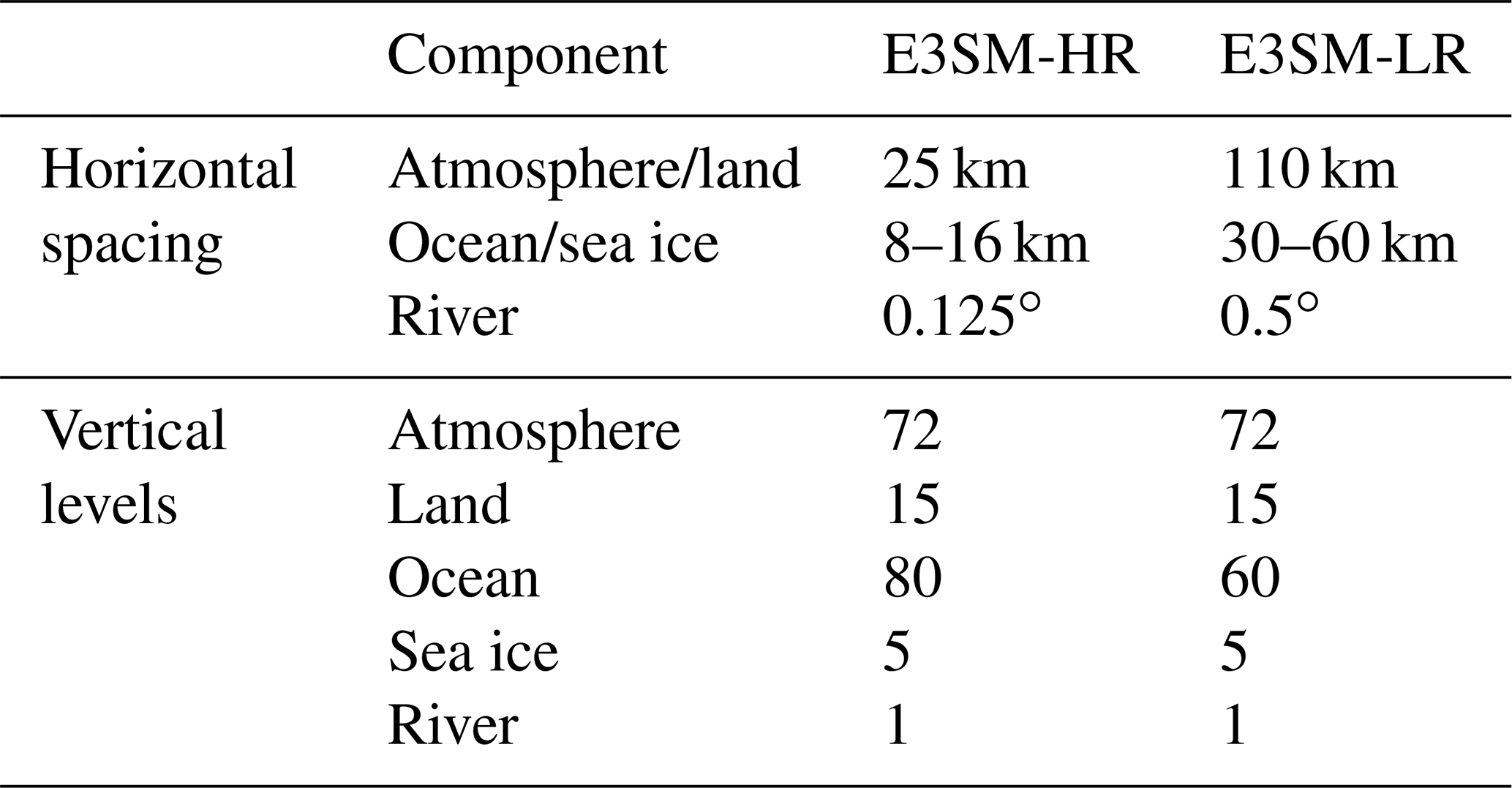
Table 1 describes the horizontal and vertical resolution for each model component. The atmosphere and land models share the same horizontal grid, having 25 and 110 km horizontal spacing for E3SM-HR and E3SM-LR, respectively. The atmospheric model uses a hybrid, sigma-pressure coordinate with 72 vertical layers and a top of the atmosphere at approximately 60 km for both the high- and low-resolution configurations. The land model uses 15 vertical levels for both simulations. For E3SM-HR, the ocean–sea ice mesh features a horizontal resolution varying between 18 km at the Equator and 6 km near the poles and 80 ocean vertical levels with spacing ranging between 2 m at the surface and ∼ 150 m at depth, following Stewart et al. (2017), to resolve the first and second baroclinic modes in the open ocean. For E3SM-LR, the ocean–sea ice mesh has a resolution varying between 60 km in the midlatitudes and 30 km at the Equator and poles, as well as 60 ocean vertical levels, with a layer thickness varying between 10 m at the surface and 250 m in the deep ocean. The river component employs a latitude and longitude grid with uniform grid spacing in both directions of 0.125 and 0.5^∘ for high and low resolution, respectively. For more detailed information on time steps and coupling frequency for each component model, refer to Table 2 in Caldwell et al. (2019).

Table 1 Horizontal and vertical resolution of E3SM-HR and E3SM-LR. In the case of sea ice, vertical levels refer to the number of thickness categories.

Before performing fully coupled simulations, we run the ocean model in stand-alone mode for 1 and 3 months for E3SM-HR and E3SM-LR, respectively, starting from rest and the Polar Hydrographic Climatology (PHC; Steele et al., 2001) temperature and salinity profiles to slightly spin up the velocity field and damp out high-velocity waves. The results of the stand-alone ocean simulation are used as the initial condition for an ocean- and sea-ice-only, 3-year simulation using the Common Ocean Reference Experiment version 2 (COREv2; Large and Yeager, 2009) protocol for interannually varying atmospheric forcing. The sea ice is initialized with a uniform thickness of 1 m at all locations south of 70^∘ S and north of 70^∘ N. Finally, the model state from the end of this simulation is used as the initial condition for the ocean and sea ice components in the fully coupled simulations. The atmospheric initial condition is obtained from an earlier high-resolution E3SM simulation run with fixed sea surface temperature (SST). The land initial condition is interpolated from the year 1950 of a low-resolution E3SM v1 CMIP simulation (Golaz et al., 2019). With these initial conditions, we run E3SM in a fully coupled model for 50 years at both high and low resolution for comparison. We use results from the last 30 years of each simulation for the analysis presented here.

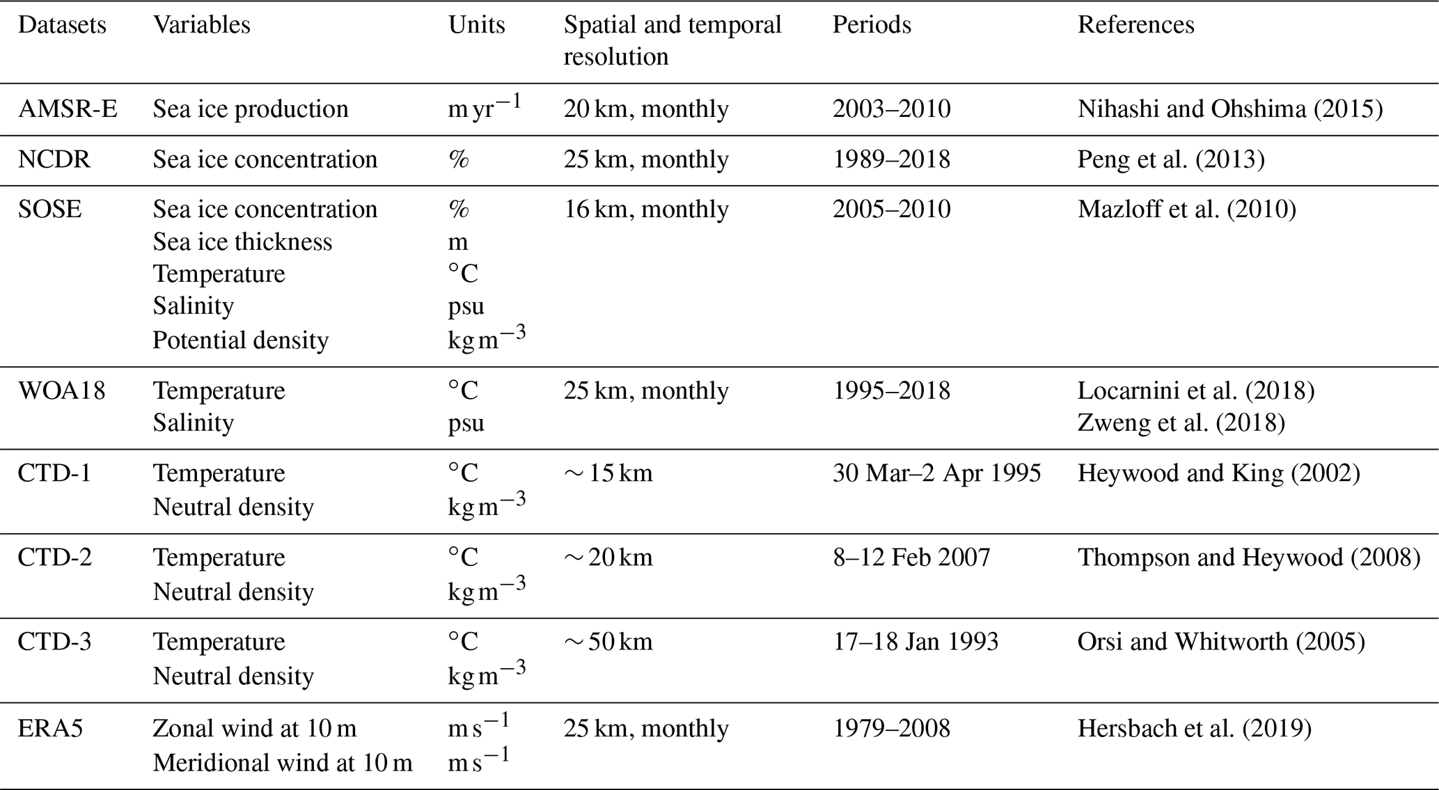
Nihashi and Ohshima (2015)Peng et al. (2013)Mazloff et al. (2010)Locarnini et al. (2018)Zweng et al. (2018)Heywood and King (2002)Thompson and Heywood (2008)Orsi and Whitworth (2005)Hersbach et al. (2019)

Table 2 Atmosphere, ocean, and sea ice state estimate datasets.

2.2 Ocean, sea ice, and atmosphere state estimates

The datasets used here for model evaluation purposes are summarized in Table 2; they include direct observations, reanalyses, and interpolated climatologies for the atmosphere, ocean, and sea ice in the Southern Ocean. For the evaluation of sea ice, we use sea ice concentration from the NOAA/NSIDC Climate Data Record of Passive Microwave Sea Ice Concentration version 3 (NCDR; Peng et al., 2013) and sea ice production from Nihashi and Ohshima (2015), which is derived from data from the Advanced Microwave Scanning Radiometer for Earth Observing System (AMSR-E). For the evaluation of oceanic currents and sea ice concentration, we utilize the Southern Ocean State Estimate (SOSE; Mazloff et al., 2010), a state-of-the-art, data assimilation product that incorporates millions of ocean and sea ice observations while maintaining dynamically consistent ocean state variables. Given the sparsity of observations in many regions around Antarctica, SOSE offers a comprehensive, physically based estimate of ocean properties that would otherwise be entirely uncharacterized (Jeong et al., 2020). Specifically, we use the SOSE dataset with $\mathrm{1}/\mathrm{6}$^∘ horizontal resolution, spanning from 2005 to 2010. We also use the World Ocean Atlas 2018 (WOA18; Locarnini et al., 2018; Zweng et al., 2018), which provides a global data product of ocean temperature, salinity, and density. Considering that both SOSE and WOA18 are based on offshore observational data, we utilize in situ conductivity–temperature–depth (CTD) observations (Heywood and King, 2002; Thompson and Heywood, 2008; Orsi and Whitworth, 2005) to better characterize the model subsurface temperature and density on the continental shelf.

For evaluating the atmospheric state over the Southern Ocean, we use zonal and meridional wind velocities at 10 m from the European Centre for Medium-Range Weather Forecasts (ECMWF) ERA5 reanalysis product (Hersbach et al., 2019). It should be noted here that the ocean, sea ice, and atmosphere datasets described above represent present-day conditions, whereas the E3SM simulations are representative of model conditions for the 1950s. We compare monthly averaged products from both present-day observations and E3SM simulations, noting that the horizontal resolution of observational datasets – varying between 16 and 25 km – differs from E3SM simulation output.

2.3 Definition of coastal polynyas and OOPs

Coastal polynyas are areas covered by “thin” sea ice, as defined by having a thickness of less than 20 cm, and surrounded by coastline and/or consolidated thick sea ice during the freezing season (e.g., Tamura et al., 2006, 2008; Nihashi and Ohshima, 2015; Ohshima et al., 2016). We apply this definition of coastal polynyas to our model results. Our definition of OOPs follows a methodology similar to previous studies (e.g., Kurtakoti et al., 2018); i.e., we consider areas within the ice pack where the open-ocean sea ice concentration is less than 15 % during the freezing season.

Table 3 The 13 major Antarctic coastal polynyas in this study.

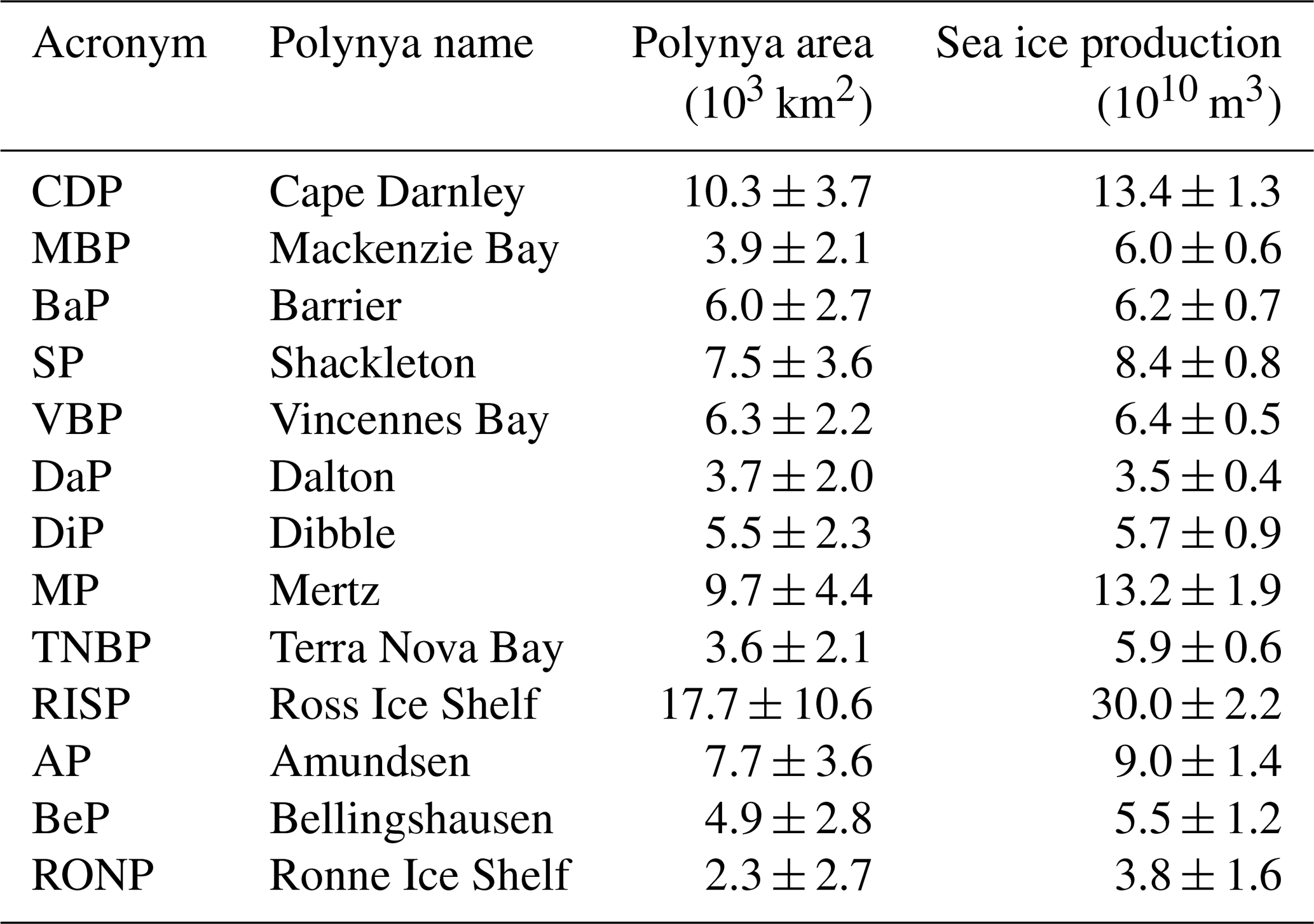
Figure 1 (a) Mean latent heat flux from the sea surface to the atmosphere (shading) and surface wind vectors during the freezing season (March–October) in E3SM-HR. Units of reference for the wind vector are meters per second (m s⁻¹). (b) Mean sea ice production rate during the freezing season (shading) and 1000 m isobath (contour) in E3SM-HR. Locations of individual coastal polynyas are shown. Definitions of abbreviations can be found in Table 3. (c) Accumulated sea ice volume as a function of longitude from Antarctic coastal polynyas from March to October from E3SM-HR (magenta) and AMSR-E (gray). (d) Total sea ice volume production per year for all Antarctic coastal polynyas for model years 26 to 55.

3 Antarctic coastal and open-ocean polynyas

3.1 Coastal polynyas

In this section, we investigate the fidelity of Antarctic coastal polynyas simulated in E3SM (a list of the 13 polynyas is included in Table 3) by comparing model output with available observational data. Cold katabatic winds blowing off Antarctica in E3SM-HR (Fig. 1a) push the thick sea ice offshore, leading to open water. Consequently, intensive latent heat flux exchanges from the ocean to the atmosphere favor sea ice production in the Antarctic coastal polynyas (Fig. 1b; note enhanced sea ice production near the Antarctic coast compared to further offshore). Sea ice volume accumulated in coastal polynyas from March to October is shown in Fig. 1c as a function of longitude for E3SM-HR and the AMSR-E satellite estimate. The AMSR-E data show that the highest rates of sea ice production occur along the East Antarctic coast, while the Ross Sea (Ross Ice Shelf polynya – RISP, around 180^∘ longitude) has the largest total sea ice production. E3SM-HR generally does well at representing the accumulated sea ice volume in coastal Antarctic polynyas, especially in high sea ice production areas along the East Antarctic coast. Furthermore, over the course of the simulation, E3SM-HR displays interannual variability in total sea ice production from Antarctic coastal polynyas of up to 43 % (Fig. 1d). This suggests that E3SM-HR may be useful for analyzing Antarctic coastal polynya variability.

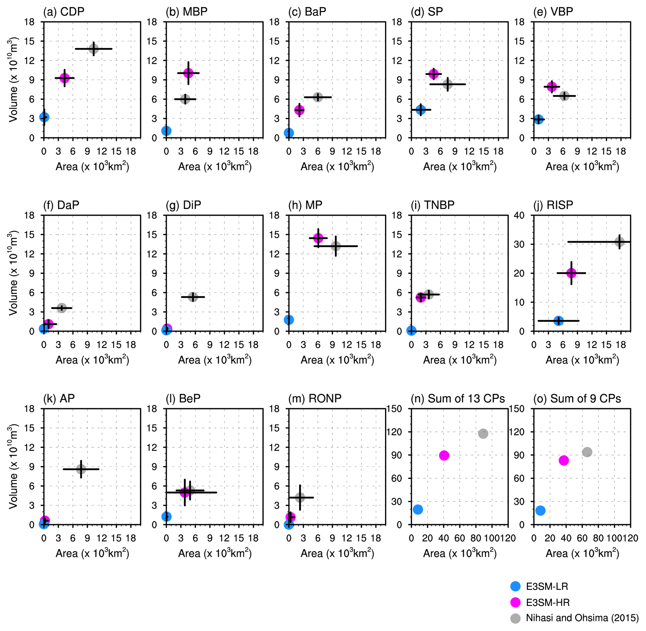
Figure 2 (a–m) Area–volume diagrams of average polynya area (x axis) and mean annual volume of sea ice production (y axis) during the freezing season from March to October for the 13 major Antarctic coastal polynyas. The black bar represents the standard deviation in the annual mean area for each coastal polynya, and the gray bar represents the standard deviation of sea ice production for each coastal polynya. Note the different scale on the y axis of panel (j). (n) Integrated polynya area and sea ice volume production for the 13 major coastal polynyas. (o) Integrated polynya area and sea ice volume production for the nine major coastal polynyas where landfast ice does not play a significant role (BaP, DaP, DiP, and AP are excluded).

The mean coastal polynya area and sea ice volume accumulated during the March to October freezing season are presented in Fig. 2 for each of the 13 polynyas indicated in Fig. 1b and Table 3; results from both the high- and low-resolution versions of E3SM are included and compared against observations. As expected, E3SM-LR shows very little polynya area or sea ice volume production over the defined coastal polynya region, whereas E3SM-HR has significant improvements in both polynya area and sea ice production compared to the low-resolution simulation. Yet, sea ice volume production in E3SM-HR is smaller than observed in several coastal polynyas such as the Dalton, Dibble, and Amundsen polynyas (DaP, DiP, AP, respectively). In reality, these coastal polynyas are strongly affected by the presence of landfast ice, a feature not yet represented in E3SM. Landfast ice is stationary sea ice attached to coastal features such as the shoreline and grounded icebergs (Nihashi and Ohshima, 2015). Several previous studies suggested that landfast ice and glacier tongues play an important role in the formation of some coastal polynyas by blocking sea ice advection of upstream sea ice into the polynya and thereby facilitating divergent motion (Nihashi and Ohshima, 2015; Bromwich and Kurtz, 1984). Therefore, a representation of landfast ice may be needed to more accurately capture coastal polynya characteristics. When we compare the sum of polynya area and sea ice volume production for polynyas that are not associated with landfast ice (Fig. 2o), it can be seen that E3SM-HR does reasonably well at reproducing sea ice volume production compared to AMSR-E observations, despite generally underestimating polynya area.

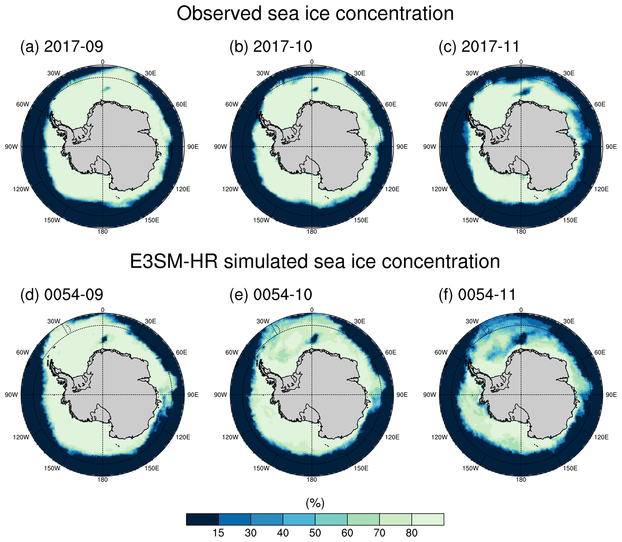
Figure 3 Observed sea ice concentration (%) during the months of (a) September, (b) October, and (c) November from NCDR (year 2017) over the Southern Ocean. Simulated sea ice concentration during the months of (d) September, (e) October, and (f) November from E3SM-HR (model year 54) over the Southern Ocean.

3.2 Open-ocean polynyas

The first observed OOP, the Maud Rise polynya (MRP), was detected during the period June to October 1973, and it propagated westward from the Maud Rise seamount into the open ocean at an average velocity of 0.013 m s⁻¹ (Gordon, 1978, 1982). In the winters of 1974 and 1975, the MRP extended westward into the central Weddell Sea, initiating a Weddell Sea polynya (WSP; Kurtakoti et al., 2018). More recently, the MRP was observed intermittently in August 2016 and more consistently during the winter of 2017 (Fig. 3a–c; note that these observations are shown for reference only and not for the purpose of model evaluation). Similarly to a previous study comparing the difference between high- and low-resolution climate model results (e.g., Dufour et al., 2017), E3SM-LR does not exhibit OOPs at any point in the simulation. E3SM-HR does produce MRPs, an example of which is shown in Fig. 3d–f for model year 54, at which relatively low sea ice concentration can be seen around 0^∘ longitude. The presence of OOPs allows the ocean and atmosphere to interact directly through enhanced exchanges of sensible heat fluxes (results not shown), potentially affecting the dense water formation in E3SM-HR.

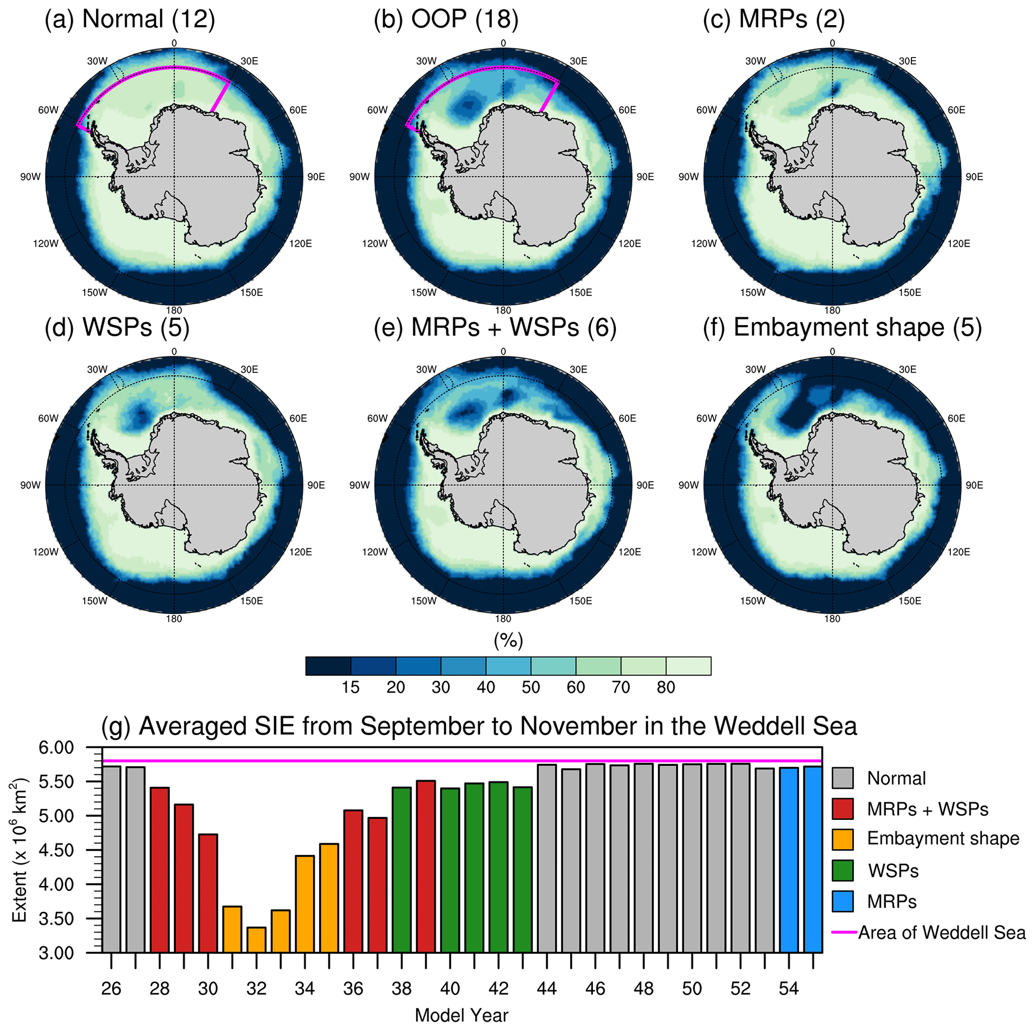
Figure 4 Composite mean of simulated sea ice concentration (%) in E3SM-HR from September to November for years with (a) no OOPs (normal year), (b) OOPs (MRPs + WSPs + embayments), (c) Maud Rise polynyas, (d) Weddell Sea polynyas, (e) Maud Rise and Weddell Sea polynyas, and (f) embayment shape cases. The numbers in parentheses are the number of years used to compute each composite analysis (years used for the composites can be found in g). The OOP years consist of all the cases of (c) Maud Rise polynyas, (d) Weddell Sea polynyas, (e) Maud Rise and Weddell Sea polynyas, and (f) embayment shapes. The pink box (a) indicates the area used to calculate the WMT rate in Sect. 4. (g) Averaged sea ice extent by E3SM model year from September to November over the Weddell Sea (pink box in a). The normal year is denoted by gray, and the OOP type is denoted by using four different colors.

OOPs appear to occur more frequently in high-resolution model simulations than in the last 50-year record of satellite sea ice observations (e.g., Kurtakoti et al., 2018; Diao et al., 2022). Even in high-resolution ocean reanalysis products, there are several cases of OOPs (for instance, in 2005 in SOSE and in 2004, 2007, and 2010 in ECCO2) that do not appear in satellite observations (Aguiar et al., 2017). The convective activity accompanying OOPs is associated with decreased stability within the water column, which can be caused by buoyancy changes in surface or deep waters (Azaneu et al., 2014). OOP formation mechanisms have been investigated extensively in the past. Most studies recognize the existence of an interplay mechanism between atmospheric wind forcing (Lockwood et al., 2021; Cheon and Gordon, 2019) and reduced upper-ocean stratification due to anomalously positive sea surface salinities that strengthens the Taylor column near the Maud Rise seamount (Kurtakoti et al., 2018; Campbell et al., 2019). In addition, a strengthening of the subpolar cyclonic gyre in the Weddell Sea may be a factor in preconditioning the oceanic convective process, since it leads to shoaling of the pycnocline and circulation that strongly interacts with the bathymetry near Maud Rise (Gordon and Huber, 1990; Azaneu et al., 2014). Possibly because of the presence of both an overly strong cyclonic gyre related to a deep subpolar low (see Sect. 4.2 below) and a reduced stratification in the Weddell Sea interior compared with WOA18 climatology (not shown), E3SM-HR produces OOPs in 18 of the 30 total simulation years (see Fig. 4), far more frequently than observed.

For the purposes of this paper, we define the simulated OOP years as those in which either or both MRP and WSP occur or in which embayment-like features in sea ice concentration occur in the Weddell Sea (Fig. 4c–f). During non-OOP years, most of the Weddell Sea is covered with sea ice from September to November (Fig. 4a). As reported elsewhere, once an OOP occurs, it has a tendency to re-occur in subsequent years (Fig. 4g) due to the ventilation of salty and high-density waters within the deep convection area that induces a positive feedback on subsequent convections (Kurtakoti et al., 2021).

4 Dense water formation

The second part of this study is to investigate dense water mass formation processes in the E3SM-HR simulation only, given that E3SM-LR does not reproduce coastal polynyas as well as OOPs and does not show signs of deep convection from inspections of the simulated mixed layer depth and upper-ocean stratification (results not shown).

4.1 Water mass transformation in OOPs and continental shelves

In this section, we apply a water mass transformation (WMT) analysis to the last 30 years of the E3SM-HR simulation in the Weddell Sea region over both the continental shelf and the open ocean to find which polynya type, coastal or OOP, predominantly produces dense water masses in E3SM-HR. The WMT analysis, first introduced by Walin (1982), quantifies the relationship between the thermodynamic transformation of water mass properties within an ocean basin and the net transport of those same properties into or out of the basin. This relationship has been used to characterize the thermodynamic processes that sustain the Southern Ocean overturning in models (Abernathey et al., 2016). A more detailed description of WMT analysis can be found in Groeskamp et al. (2019). Jeong et al. (2020) discuss previous applications of WMT to the analysis of low-resolution E3SM simulations.

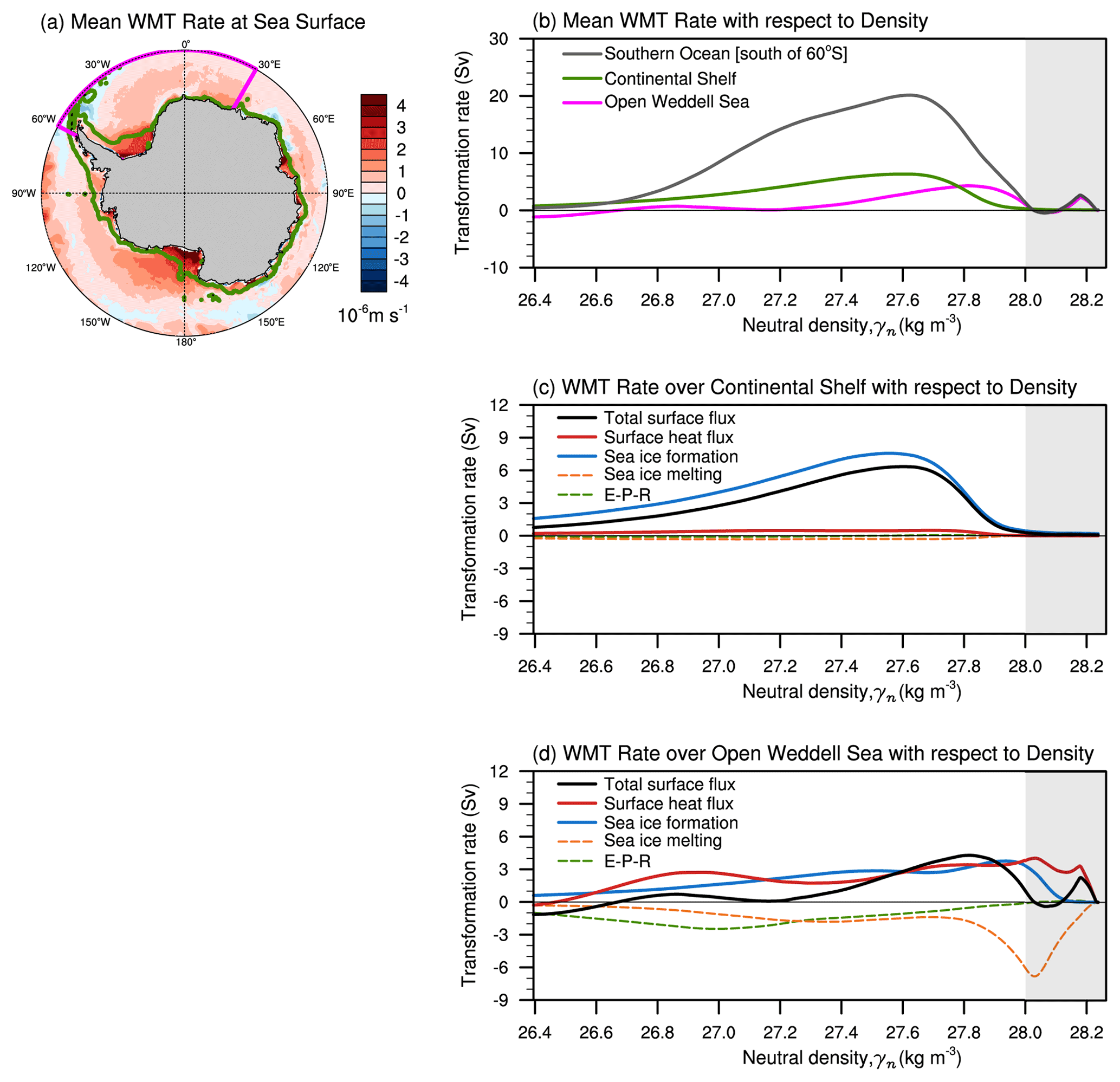
Figure 5 (a) The 30-year mean water mass transformation (WMT) rate integrated over all density classes from March to October (freezing season) by total surface fluxes, including surface heat and freshwater fluxes from the E3SM-HR simulation. The green bold contour marks the 1000 m isobath (which defines the continental shelf here), and the pink box in (a) identifies the Weddell Sea as defined in this study. (b) WMT rates with respect to neutral density class summed over the whole Southern Ocean (gray), continental shelf (green), and Weddell Sea (pink). Note that the green and pink curves do not sum to the gray curve. Panels (c) and (d) show WMT rates driven by the total surface flux and its components integrated over the continental shelf and over the open Weddell Sea, respectively. The WMT rate driven by the total surface flux (solid black) consists of those induced by surface heat flux (solid red), freshwater flux from sea ice formation (solid blue), sea ice melting (dashed orange), and E–P–R (dashed green; evaporation, precipitation, and runoff).

In Fig. 5a, we show the mean WMT rate over the Southern Ocean produced in E3SM-HR for all surface fluxes combined (positive WMT rates indicate that water masses become denser, implying buoyancy loss; negative WMT rates indicate that water masses become lighter, implying buoyancy gain). Because we only focus on the WMT rate during the freezing season from March to October, positive WMT rates dominate over most of the Southern Ocean. Over the continental shelf, the region delimited by the 1000 m isobath in Fig. 5a, we find strong positive WMT rates, which are the direct result of high sea ice production there (Fig. 1b). These results compare well in magnitude with observation-based estimates (Pellichero et al., 2018).

The mean WMT rates in latitude and longitude space can be converted into neutral density space and are shown in Fig. 5b for the whole Southern Ocean (gray line), the continental shelf only (green line), and the Weddell Sea (pink line). The maximum WMT rates over the whole Southern Ocean (≈ 20 Sv) are found at a neutral density of 27.6 kg m⁻³ and are larger than the observation-based estimate (≈ 13 Sv) in Pellichero et al. (2018). In the high density ranges above 28.0 kg m⁻³, a local maximum WMT rate of 3.0 Sv is seen at a neutral density of 28.2 kg m⁻³. Whitworth et al. (1998) and Orsi et al. (1999) define AABW as having neutral densities higher than 28.27 kg m⁻³. We consider 28.0 kg m⁻³ to be a suitable minimum threshold of AABW in the E3SM-HR simulation. As this high-density transformation rate in E3SM-HR is entirely due to WMT over the Weddell Sea rather than on the continental shelf (compare green and pink lines in Fig. 5b), the simulated bottom water is produced through open-ocean convection in the Weddell Sea only, similarly to what has been found in previous studies (Heuzé et al., 2013; Azaneu et al., 2014; Aguiar et al., 2017). Over the continental shelf, we also see positive transformation rates, but these occur at relatively lighter densities, with an average neutral density of 27.5 kg m⁻³, whereas no transformation occurs at densities higher than 28.0 kg m⁻³. These results are confirmed by the T–S diagrams for the Weddell Sea water column, presented in Fig. S1 in the Supplement and computed from both the E3SM-HR annual climatology and the WOA18 climatology. Compared to WOA18 and also considering Fig. 1a in Whitworth et al. (1998), E3SM-HR exhibits a reasonably well-reproduced CDW and Antarctic surface water, but it misses shelf waters completely and produces AABW that is less dense (mostly because it is less cold) than observed.

When we consider the WMT rate contributed by several types of surface fluxes separately over the Antarctic continental shelf and over the Weddell Sea (Fig. 5c and d), the positive transformation rate over the continental shelf results almost entirely from brine rejection by sea ice production. The positive WMT rate over the deep Weddell Sea, meanwhile, is mostly due to the surface heat release from the ocean to the atmosphere, especially at relatively high neutral densities above 28.0 kg m⁻³, which is consistent with the strong ocean-to-atmosphere exchanges that occur in OOPs. We confirm, therefore, that the coastal polynyas and OOPs simulated in E3SM-HR have different WMT mechanisms. However, as described above, the simulation produces water masses at relatively low density levels on the continental shelf, despite the fact that the model does reasonably well at reproducing a large amount of sea ice formation in coastal polynyas during the freezing season. To investigate this apparent inconsistency, in the next section we examine E3SM-HR's hydrographic characteristics in the Southern Ocean.

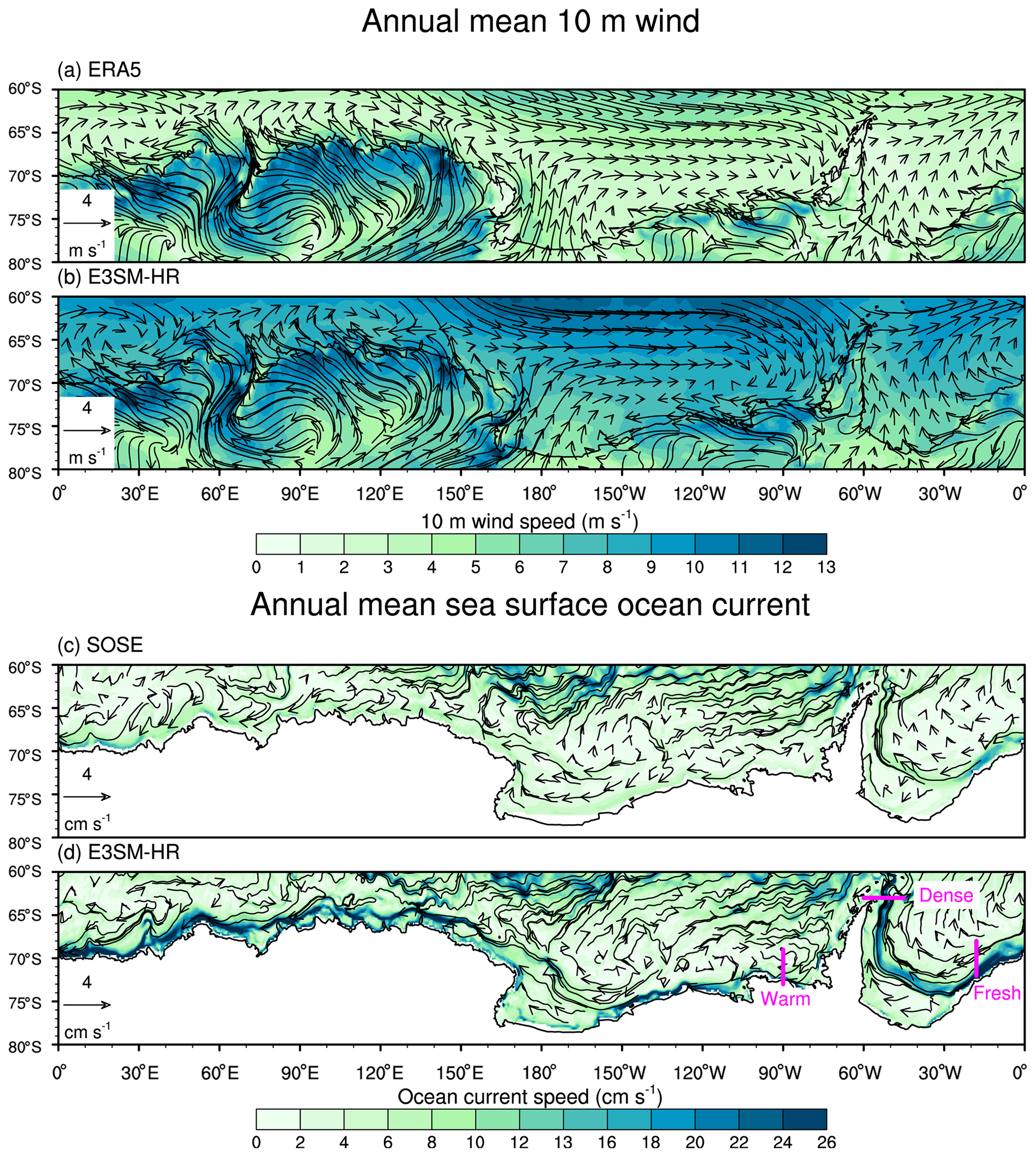
Figure 6 Annual mean atmospheric surface winds (at 10 m) from (a) ERA5 and (b) E3SM-HR. Annual mean sea surface ocean currents from (c) SOSE and (d) E3SM-HR. Shading represents the speed of atmospheric winds and ocean currents. The locations for each shelf type are indicated by “warm”, “dense”, and “fresh” in (d) to represent warm, dense, and fresh shelves, respectively.

4.2 Hydrographic characteristics of continental shelves

We start by comparing E3SM-HR's atmospheric surface (10 m) winds with the ERA5 reanalysis data (Fig. 6a and b). Compared to ERA5, E3SM-HR has stronger atmospheric surface winds, not only along the Antarctic continental shelf but also in the interior Southern Ocean, which is consistent with an overly deep subpolar low-pressure system south of 60^∘S (Fig. S2 in the Supplement). The overly strong atmospheric winds along the continental shelf may impact the strength of the ASC. Indeed, in Fig. 6c and d, we find that a very strong ASC is simulated in E3SM-HR, with speeds more than double those in SOSE (e.g., 0.34 m s⁻¹ in E3SM-HR compared with 0.16 m s⁻¹ in SOSE at 0^∘ longitude). Therefore, we hypothesize that the strong winds over the continental shelf may be one of the drivers of the strong ASC in E3SM-HR.

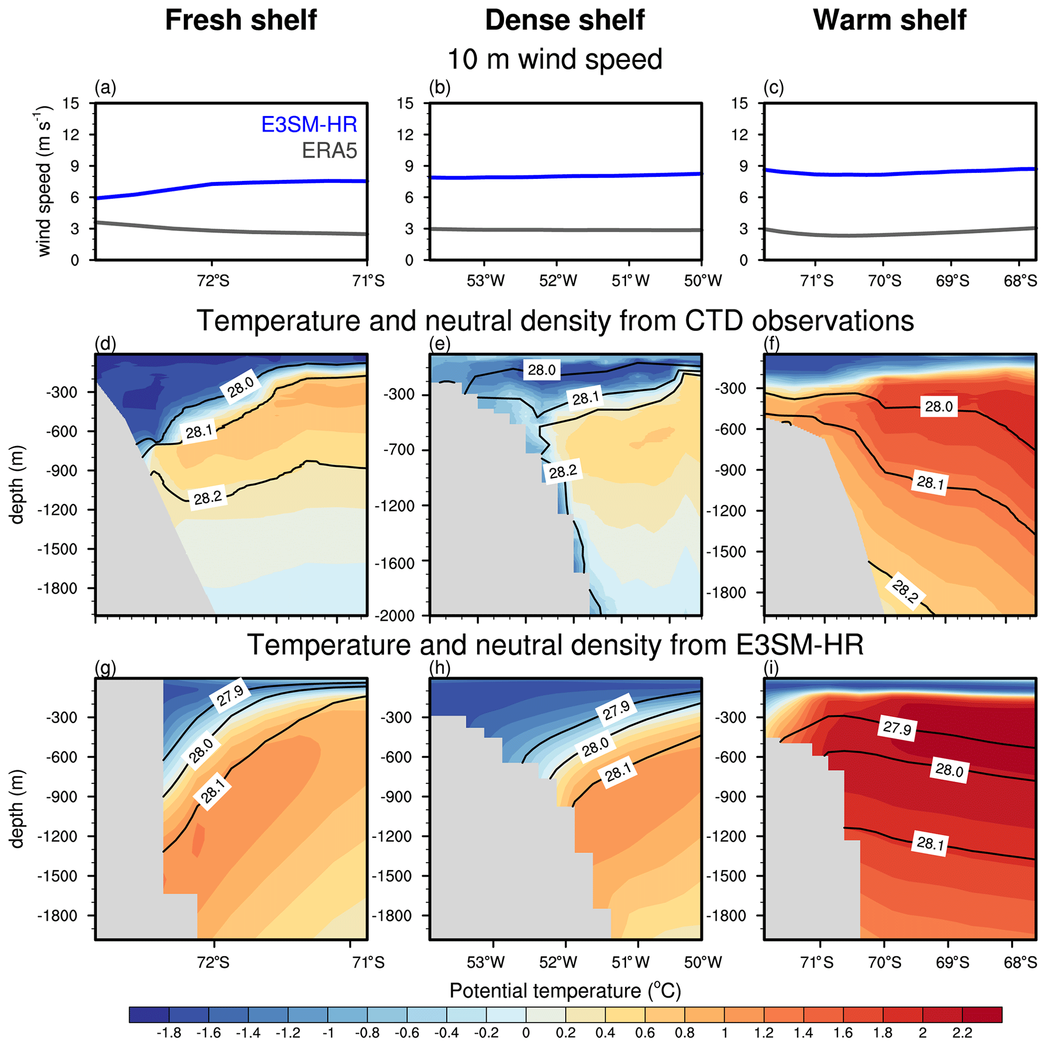
Figure 7 (a–c) Atmospheric wind speed at 10 m from ERA5 and E3SM-HR. (d–f) Measurements of conservative temperature (colors) and neutral density (black contours) across the ASC in locations corresponding to each ASC regime: (d) the eastern Weddell Sea (Heywood and King, 2002), (e) the western Weddell Sea (Thompson and Heywood, 2008), and (f) the Bellingshausen Sea (Orsi and Whitworth, 2005). (g–i) Vertical cross-section of ocean temperature (colors) and neutral density (black contours) from an annual average of the E3SM-HR simulation. The left (a, d, and g), middle (b, e, and h), and right (c, f, and i) columns show an example of fresh, dense, and warm shelf cases. Section locations are shown in Fig. 6.

A closer look at the shelf hydrography supports this hypothesis. In particular, we select three vertical meridional and zonal cross-sections at 18^∘W (eastern Weddell Sea), 63^∘ S (western Weddell Sea), and 90^∘ W (Bellingshausen Sea), which are representative of the fresh, dense, and warm shelf types, respectively (the locations of the cross-sections are indicated in Fig. 6d, and they coincide with the sections described in Thompson et al. (2018). The results are presented in Fig. 7, comparing the model temperature and density profiles with CTD observational data (Heywood and King, 2002; Thompson and Heywood, 2008; Orsi and Whitworth, 2005). In general, E3SM-HR features down-sloping isopycnals approaching the continental slope in all cross-sections. For the fresh shelf type (Fig. 7a, d, and g), the model isopycnal surfaces are strongly tilted downwards in the onshore direction, more so than in the observational results (Fig. 7d). The strong Antarctic Slope Front (ASF) in the fresh shelf may be induced by the higher easterly winds (with respect to ERA5 winds) along this shelf (Fig. 7a). At the dense shelf type (Fig. 7b, e, and h), the isopycnals associated with warm CDW tilt down toward the seafloor over most of the continental slope. However, as the CDW approaches the shelf break in the dense shelf type, the observed isopycnals shoal again, indicating a V-shaped isopycnal surface (Fig. 7e). Unlike observations, E3SM-HR exhibits no V-shaped isopycnals, but rather steep isopycnal surfaces tilted downward toward the shelf break from offshore. This is also likely related to overly strong model winds (Fig. 7b). Lastly, in the warm shelf type (Fig. 7c, f, and i), the observations show isopycnal surfaces that tilt upward towards Antarctica, resulting in warm CDW reaching the continental shelf (Fig. 7f). Again, E3SM-HR simulates hydrographic conditions that are more similar to the fresh shelf type, with downward-tilted isopycnals (Fig. 7i). This bias could similarly be related to the overly strong model winds (Fig. 7c).

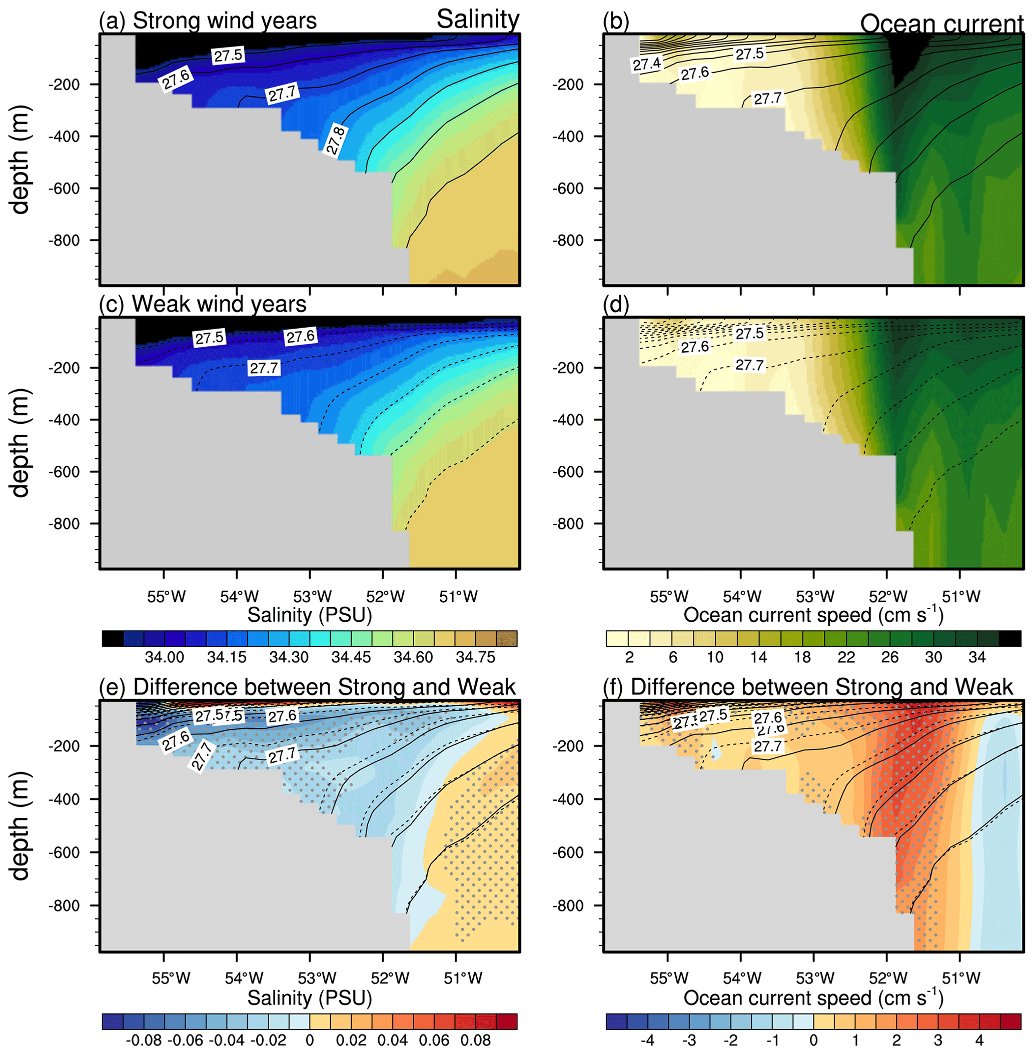
Figure 8 (a, c, and e) Vertical cross-section of salinity (shading) and neutral density (contour lines) for (a) strong wind years, (c) weak wind years, and (e) difference between strong and weak wind years from E3SM-HR simulation. (b, d, f) Vertical cross-section of ocean current speed (shading) and neutral density (contour lines) for (b) strong wind years, (d) weak wind years, and (f) the difference between strong and weak wind years from the E3SM-HR simulation. For the differences, statistically significant values (P < 0.05) are stippled.

To further support our hypothesis that strong winds are responsible for the strong ASF, we compare vertical cross-sections of salinity, neutral density, and ocean current speed for the dense shelf case and for a strong wind and a weak wind composite (Fig. 8). The strong wind (weak wind) composite was computed by selecting all years with the top (bottom) 25 % winter wind speeds over the dense shelf (63^∘ S). Compared to weak wind years, strong wind years are characterized by a pronounced subsurface salinity cross-section gradient between the relatively salty waters in the CDW layer and the fresher waters over the continental shelf (Fig. 8e). In response to the lateral gradient in salinity, the lateral density gradient is also strong in the strong wind years, which causes an intensification of the ASC and ASF at or close to the shelf break (Fig. 8f). These results further indicate that the wind bias is the main contributor to the strong ASC in the E3SM-HR simulation.

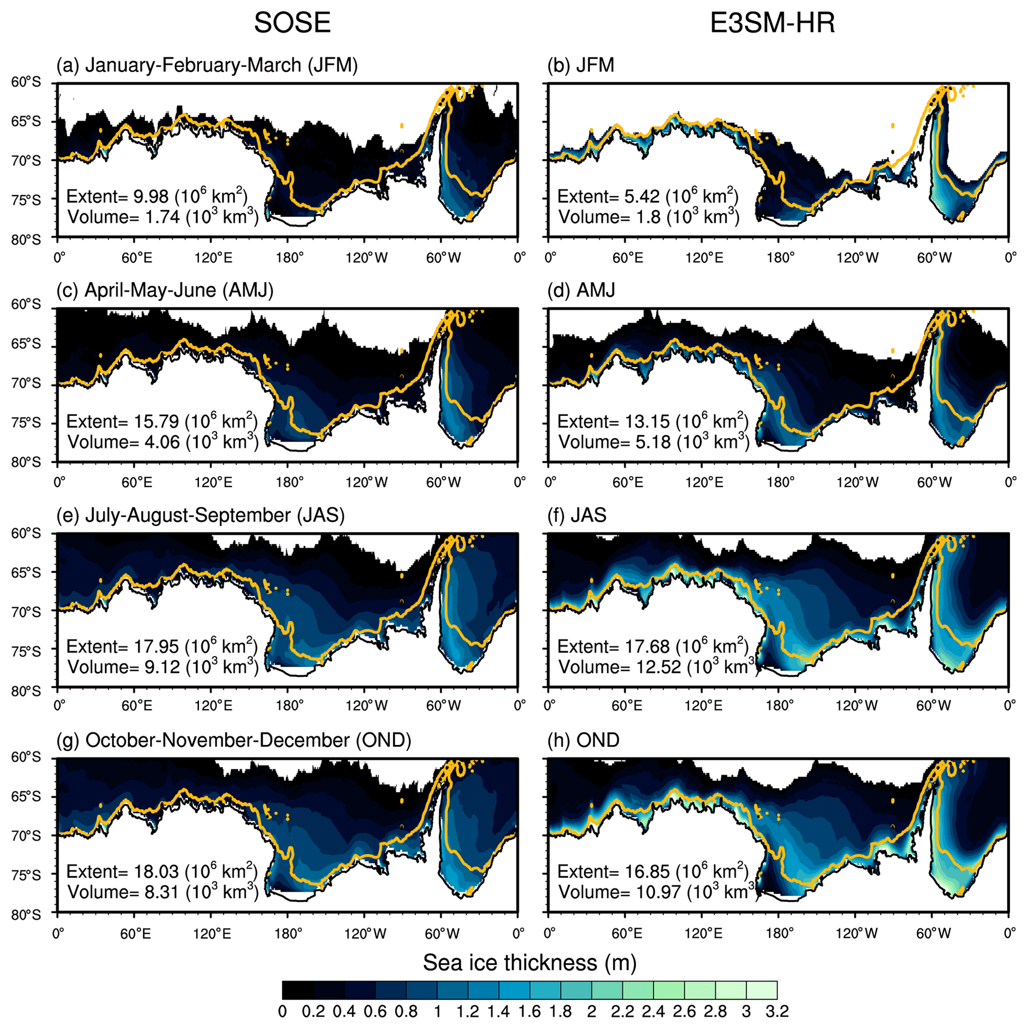
Figure 9 Seasonal mean sea ice thickness during JFM (January–February–March), AMJ (April–May–June), JAS (July–August–September), and OND (October–November–December) from (a, c, e, g) SOSE and (b, d, f, h) E3SM-HR. The region where sea ice concentration is less than 15 % is masked out. The yellow contour line denotes the 1000 m isobath. Sea ice extents and volumes for each season are also displayed.

In summary, as a result of ubiquitous, strong polar easterly winds, we find that E3SM-HR consistently displays only the fresh shelf type. These overly strong winds cause enhanced onshore Ekman transport (see Fig. S3 in the Supplement, particularly the shelf results in panel c), which in turn may affect the advection of sea ice formed during the winter season. As shown in Fig. 9, E3SM-HR's simulated sea ice extent in the Southern Ocean is much less than that from SOSE in all seasons except for JAS (July–August–September), but sea ice volume is generally larger than SOSE's, and the largest differences are found in the coastal regions. We hypothesize that this is the result of sea ice build-up on the continental shelf in E3SM-HR, wherein sea ice thickness often exceeds 2 m, due to enhanced poleward surface Ekman transport, which prevents sea ice from moving to lower latitudes where it would potentially melt.

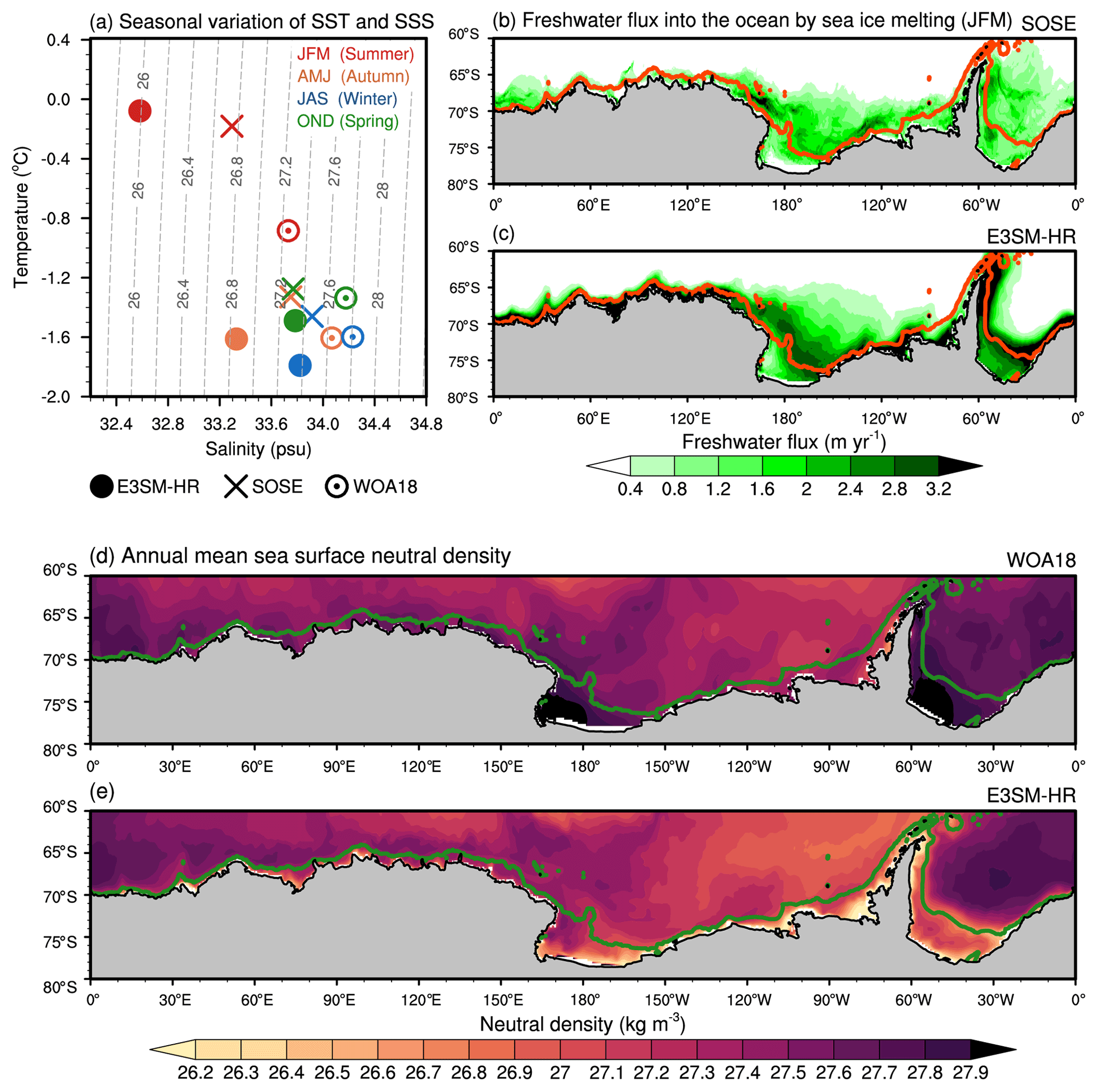
Figure 10 (a) Seasonal and area-averaged sea surface temperature (SST) and sea surface salinity (SSS) from E3SM-HR, SOSE, and WOA18 over the continental shelves for the season of January–February–March (JFM, summer), April–May–June (AMJ, autumn), July–August–September (JAS, winter), and October–November–December (OND, spring). Dashed lines on the T–S diagram are neutral density contours. Seasonal mean freshwater flux into the ocean by sea ice melting for JFM from (b) SOSE and (c) E3SM-HR. Annual mean sea surface neutral density from (d) WOA18 and (e) E3SM-HR. Red (b, c) and green (d, e) bold contours represent the 1000 m isobath.

Modeled and observed SST and sea surface salinity (SSS) averaged over the continental shelf provide additional information regarding the impacts of these biases. In Fig. 10 we compare shelf SST and SSS from E3SM-HR with those from SOSE and WOA18. E3SM-HR has a good representation of seasonal SST and SSS variation, but with warmer and fresher as well as colder and fresher water properties in the summer and winter seasons, respectively, compared to SOSE and WOA18. In summer, the warm, fresh surface water has a neutral density of 26.0 kg m⁻³ in E3SM-HR compared with more than 27.2 kg m⁻³ in WOA18 and 26.8 kg m⁻³ in SOSE. The possible external sources of the relatively low summer density in E3SM-HR can be excessive precipitation (E-P), runoff, or sea ice melting. Consistent with the sea ice thickness bias discussed above (Fig. 9), we find that the freshwater flux into the ocean from melting sea ice in E3SM-HR is larger than that of SOSE, especially over the continental shelf and shelf break (Fig. 10b), while precipitation and runoff differences (not shown) are not significant compared to SOSE. Because of extensive and excessive freshwater inputs from sea ice in E3SM-HR, the annual mean sea surface neutral density is lighter than WOA18 over the continental shelf (Fig. 10d and e). We thus conclude that the overly strong easterly winds are also (indirectly) responsible for the relatively lighter water masses forming on the continental shelf in E3SM-HR.

5 Discussion

There are several phenomena known to be important in the physics associated with coastal polynyas that are challenging to model. Perhaps most importantly, the ASC and its associated cross-shelf stratification play a critical role in establishing water mass and heat transport on and off the Antarctic shelf, as well as in the Earth's climate system in general through their effects on the large-scale ocean circulation, the stability of Antarctic ice sheets, and the global carbon cycle (Thompson et al., 2018). While the ASC is largely absent in low-resolution E3SM simulations (Jeong et al., 2020), it has a much-improved representation in E3SM-HR. This is likely due to the higher resolution of the simulated surface winds, the use of higher-resolution bathymetry, and better reproduction of mesoscale eddy activity over the Antarctic continental slope. Yet, it should be noted that resolution much higher than the 6 km available in the ocean component of E3SM-HR around Antarctica is needed to fully resolve the mesoscale eddies on the continental shelf (resolutions of at least 2 km very near the coast; see, e.g., Hallberg, 2013). Furthermore, the results presented in this paper have indicated the presence of an overly strong ASC around Antarctica in E3SM-HR, associated with overly strong alongshore winds, particularly in dense shelf and warm shelf regions. This suggests that high horizontal resolution in the ocean and atmosphere models alone cannot guarantee a better representation of the ASC, but a realistic simulation of the alongshore winds is also an important factor. The E3SM wind biases over the Southern Ocean have been substantially reduced in E3SM version 2 through aggressive tuning of boundary layer turbulence mixing and surface flux exchange (results not shown). In future studies, we plan to further investigate and understand the impact of winds by exploiting the latest version of E3SM. The ASC also depends on tidal flow across the continental shelf break (Stewart et al., 2019), and that is another process currently missing in our ocean model. Another important but missing piece in E3SM-HR is the representation of ice shelves, which closely interact with coastal polynya and DSW formation (Jeong et al., 2020). Landfast sea ice effectively modifies the coastline, thus affecting the location and extent of coastal polynyas (e.g., Lemieux et al., 2018). Although this process is currently missing in E3SM, an explicit physical model of landfast sea ice is in the planning stages. Finally, the E3SM sea ice dynamics modeled along the coast also possess no tensile strength or interaction with icebergs, but both are known to be important for shaping coastal polynyas (Fraser et al., 2012). We intend to explore the impacts of tides, landfast ice, and icebergs on polynya formation in future studies using E3SM.

Coupled GCMs are sophisticated tools designed to simulate, understand, and predict the behavior of the Earth's climate system (Laloyaux et al., 2016). However, the model validation or assessment of climate phenomena from coupled GCMs has traditionally been compared with uncoupled reanalysis data, as we have done in this study. We may have over-interpreted biases in E3SM relative to uncoupled reanalysis products, given that they also have their own biases, in part because they lack physics-based constraints. Hence, there is a need for methods that are designed to process observations of the atmosphere and ocean in a coupled model in a consistent manner (Laloyaux et al., 2016). Improvements in model capabilities and increases in computing power are enabling the analysis of the Earth's climate system using such fully coupled data assimilation schemes (Penny et al., 2019), and future assessments of E3SM would greatly benefit from such coupled model reanalysis products. Different temporal and spatial resolutions also introduce discrepancies between observations or reanalysis products and model results. A potential caveat to note is that we only used one high-resolution and one low-resolution model simulation, thus not providing a quantification of structural model uncertainty.

The E3SM simulations presented in this paper use the fixed 1950s atmospheric forcing, which consists of greenhouse gases, O₃, and aerosol for a 1950s (∼ 10-year mean) climatology. Therefore, the E3SM simulation reflects the internal variability of a stable climate. The observations with which E3SM-HR is compared are for a transient climate. They cover the period from 1979 onwards, but they are mostly from the current century, which is at a significantly different point in the industrial epoch than is represented in our 1950s trace atmospheric model constituents. However, previous studies (e.g., Santer et al., 2008; Notz et al., 2013; Swart et al., 2015) indicated that the trends or mean values in observations and individual model simulations may differ significantly because of internal variability rather than differences in response to the external forcing. In addition, Menary et al. (2018) and Jeong et al. (2020) found that the differences between preindustrial and present-day control simulations are much smaller than the differences between different model configurations under the same preindustrial or present-day forcing. Finally, we note that E3SM-HR uses an Antarctic land–sea boundary based on data from the 1990s and 2000s, which includes floating ice tongues that are important for determining the locations of coastal polynyas (and which are also present in the observations used in this study). For all of these reasons, we feel justified in using present-day observations as a metric by which to judge our model output.

6 Summary and conclusions

In this paper, we have investigated dense water formation in Antarctic coastal polynyas and OOPs using the fully coupled E3SM-HR and E3SM-LR simulations. In terms of sea ice area and sea ice volume, we find that E3SM-HR reproduces the main features of the 13 most important Antarctic coastal polynyas. There are limitations, however, with the representation of several coastal polynyas, which are possibly related to E3SM's current inability to represent landfast ice. This suggests that adding an accurate representation of landfast ice in E3SM-HR will be essential for correctly simulating coastal polynya and for future studies of polynya variability. E3SM-HR also reproduces MRPs, which were observed in the winters of 2016 and 2017, as well as prior to that in the 1970s. The model shows good agreement with satellite observations of the 2017 areal extent and time evolution of the MRP. E3SM-HR frequently produces several other types of OOPs, such as the WSP, concurrent MRP and WSP events, and embayment-shaped polynyas. Aside from the latter, all of these were observed in the 1970s.

We subsequently investigated dense water formation in E3SM-HR on the continental shelf and in the Weddell Sea using WMT analysis. We found significant positive WMT rates on the Antarctic continental shelf, which are almost entirely due to brine rejection by sea ice formation there. However, the positive WMT rates occur at lower densities than expected. Instead, the densest water masses are formed in the interior Weddell Sea when heat is transferred from the deep ocean to the surface and then to the atmosphere during OOP events.

We found that E3SM-HR has overly strong polar easterlies, resulting in a strong ASC separating cold and fresh water nearly everywhere on the continental shelf from warm and salty CDW further offshore. Anomalously strong polar easterlies also lead to overly strong southward surface Ekman transport, sea ice build-up near the coast, and consequent excessive sea ice melting on the continental shelf in the summer season. This in turn is mostly responsible for the ambient density of seawater on the continental shelf being too low throughout the year in E3SM-HR, producing a large density contrast between the continental shelf and waters further offshore. On the other hand, in the interior Weddell Sea, E3SM-HR allows for an alternative method of deep ocean ventilation via deep ocean convection, strong air–sea interactions, and dense water formation during OOP events, consistent with findings from previous modeling studies (Azaneu et al., 2014; Aguiar et al., 2017; Kurtakoti et al., 2018).

The strong polar easterlies in E3SM-HR are due to an overly deep subpolar low-pressure system around 60–70^∘ S, which also causes an intensification of the cyclonic ocean circulation in the Weddell Sea (Weddell Gyre). Studies of WSPs (e.g., Cheon et al., 2014) suggest that the intensification of the Weddell Gyre is one of the possible preconditioning mechanisms for WSPs due to the Ekman pumping and raising of isopycnals in the center of the gyre. Thus, overly deep subpolar low-pressure systems may impact both OOP phenomena and the water mass formation occurring in coastal polynyas.

Regardless of the biases described above, we have shown here that fully coupled, high-resolution E3SM simulations can partially reproduce Antarctic coastal polynyas, an important advancement given their importance as a source of AABW formation and that AABW formation processes are currently underrepresented or misrepresented in most ESMs. Silvano et al. (2018) suggest that increased submarine melting of Antarctic ice shelves may reduce AABW formation by offsetting salt fluxes during sea ice formation in coastal polynyas, a change that could then prevent full-depth convection and the formation of dense shelf water. This hypothesis is supported by the simulations and WMT analyses of Jeong et al. (2020), wherein the impacts of explicitly including submarine ice shelf melt fluxes in a low-resolution ESM were explored. Future work should focus on better understanding the impacts of both high spatial resolution and sub-ice-shelf melting on simulations of Antarctic coastal polynyas, dense water formation, ocean stratification, and the potential feedback between these processes.