Uncertainty analysis of single- and multiple-size-class frazil ice models

The formation of frazil ice in supercooled waters has been extensively studied, both experimentally and numerically, in recent years. Numerical models, with varying degrees of complexity, have been proposed; these are often based on many parameters, the values of which are uncertain and difficult to estimate. In this paper, an uncertainty analysis of two mathematical models that simulate supercooling and frazil ice formation is carried out within a probabilistic framework. The two main goals are (i) to provide quantitative insight into the relative importance of contributing uncertain parameters, to help identify parameters for optimal calibration, and (ii) to compare the output scatter of frazil ice models with single and multiple crystal size classes. The derivation of single- and multi-class models is presented in light of recent work, their numerical resolution is discussed, and a list of the main uncertain parameters is proposed. An uncertainty analysis is then carried out in three steps. Parameter uncertainty is first quantified, based on recent field, laboratory and numerical studies. Uncertainties are then propagated through the models using Monte Carlo simulations. Finally, the relative influence of uncertain parameters on the output time series – i.e., the total frazil volume fraction and water temperature – is assessed by means of Sobol indices. The influence of input parameters on the long-term asymptote as well as short-term transient evolution of the systems is discussed, depending on whether gravitational removal is included or not in the models.

1 Introduction

Formation of frazil ice in water bodies has been widely investigated because of its impact on submerged structures (Daly, 1991, 2006; Richard and Morse, 2008) and because it often precedes formation of ice cover in rivers and oceans (Daly, 1994; Smedsrud and Jenkins, 2004). Frazil ice also plays an important role in geophysical flows such as plumes of ice shelf water under floating ice sheets (Bombosch and Jenkins, 1995; Rees Jones and Wells, 2018; Frazer et al., 2020). For these reasons, the study of frazil formation processes is an active area of research, with a large variety of applications in river and coastal engineering.

The main drivers for the formation of frazil are the water cooling rate resulting from heat exchanges with the atmosphere, the initial seeding of frazil nuclei and the turbulent mixing. Then, the thermal growth process deriving from the heat exchange between water and primitive crystals allows a fine description of the balance between growth frazil ice and water supercooling. Previous mathematical models describing the evolution of frazil ice and water temperature were based on ideas pioneered by Daly (1984, 1994). Omstedt (1985) developed a model based on a turbulent channel-flow boundary layer theory, in which a mean particle of constant geometric properties and constant Nusselt number is considered. Mean particle-size models have been incorporated in numerical hydraulic tools such as CRISSP2D (Shen and Wasantha Lal, 1993; Shen et al., 1995; Shen, 2010). More complex models are based on the ice-number continuity equation introduced by Daly (1984), taking into account the complexity of crystal distribution. In contrast with single-size-class models, the crystal number continuity equations allow introduction of secondary nucleation and flocculation processes. When combined with thermal growth, these complement the modeling of frazil crystal size evolution. Svensson and Omstedt (1994) proposed a numerical model for solving the equations introduced by Daly (1984) by considering discrete radius intervals. Conceptual models for secondary nucleation and flocculation were introduced and calibrated to fit the experimental data of Michel (1963) and Carstens (1966). Hammar and Shen (1991) derived a variable particle-size model in two dimensions and later improved it with secondary nucleation and flocculation (Hammar and Shen, 1995). Variable particle-size models have also been integrated in TELEMAC-MASCARET (Souillé et al., 2020). Numerous simplified implementations have been made that consider a well-mixed water body. For example, Wang and Doering (2005) worked with the same model as Svensson and Omstedt (1994) and further discussed calibration of influential parameters in initial seeding, secondary nucleation, and flocculation by comparing them with the experimental data of Clark and Doering (2004). Implementation of multiple-size-class frazil dynamics in the context of sea ice and ice shelf water plumes has also been proposed by Smedsrud (2002), Smedsrud and Jenkins (2004) and Holland and Feltham (2005). In the same context, Rees Jones and Wells (2018) have recently shed new light on multiple-size-class models and discussed crystal growth rate and the occurrence of frazil explosion. They also identified and characterized the steady-state crystal size distribution. Henceforth, single- and multiple-size-class models will be referred to as SSC (single size class) and MSC (multiple size class) models respectively.

Common to all numerical model of frazil dynamics is their use of a large number of parameters, making calibration difficult. The modeling studies mentioned above show that frazil ice models can be fitted to reproduce the evolution of temperature and frazil volume fraction. However, given the uncertainty of fitting parameters, it is questionable whether these models are predictive. As Rees Jones and Wells (2018) point out, the consistency between experiments and models does not necessarily mean parameterization is correct. This is particularly true when different processes compete and have similar impact on the crystal size distribution. Besides, introducing new processes in the models increases the number of parameters that need calibration. This comes at the cost of introducing new uncertain parameters and raises the question of models trustworthiness.

This trade-off between uncertainties and model complexity is often discussed in geophysical and environmental modeling (MacGillivray, 2021; Van Zelm and Huijbregts, 2013). On this matter Saltelli (2019) advises use of statistics to aid mathematical modeling via “a systemic appraisal of model uncertainties and parametric sensitivities”. There is, moreover, a growing appreciation of how sensitivity analysis enhances the understanding of the intricate physical processes involved in ice formation (Sheikholeslami et al., 2017). The sensitivity of multiple-size-class frazil models to initial seeding, secondary nucleation and flocculation parameters has been investigated by Wang and Doering (2005) and Smedsrud and Jenkins (2004), by simple modifications of specific parameters. Although probabilistic methods are sometimes used in processing observational data (Frazer et al., 2020), to the author's knowledge, probabilistic sensitivity analysis of frazil ice models has never been performed. In addition, comparison of SSC and MSC models in terms of uncertainty of output has never been tackled, despite the prohibitive computational cost of the MSC model, making the SSC approach still relevant to many applications.

In this paper, we intend to bridge that gap by proposing an uncertainty and sensitivity analysis of single and multiple-class frazil ice models, using a of full description of parameters uncertainty (by probability density functions) and variance decomposition of model outputs. First, we introduce the models and main hypotheses and discuss their implementation in Sect. 2. The uncertainty assessment methodology is presented in Sect. 3. We then rely on numerous field and experimental measurements to quantify the uncertainties of input parameters of the two frazil numerical models in Sect. 4. Using Monte Carlo experiments, we next study the propagation of these uncertainties on model outputs in Sect. 5: in other words, the evolution of the frazil ice volume fraction and the water temperature. The evolution of output scatter is discussed and compared to the asymptotes of the dynamic systems. Finally, sensitivity analysis based on Sobol indices (Sobol, 2001) and aggregated Sobol indices enables us to propose a selection of the most influential parameters in both models. We conclude with this study's perspectives in Sect. 6.

2 Frazil ice dynamics

This section introduces the continuum equations used to describe evolution of water temperature and frazil volume fraction, as well as their discrete counterparts and their numerical resolution under the assumption of well-mixed water bodies. The parameters of the models that can be considered uncertain are also introduced.

2.1 Mathematical description

Frazil crystals are assumed to be discs of radius r and thickness λ. The ratio between diameter and thickness, denoted $R=\mathrm{2}r/\mathit{\lambda }$, is supposed to be constant as crystals grow. Let us define n as the crystal number density, which corresponds to the number of crystals per unit volume per unit length in radial space. The total number of particles per unit volume is then defined as $N=\underset{\mathrm{0}}{\overset{\mathrm{\infty }}{\int }}n\left(r\right)\mathrm{d}r$. We also introduce the frazil volume fraction density as c=nV, in which V=πr²λ is the crystal volume. The volume proportion of the water–ice mixture occupied by frazil ice, i.e., the total volume fraction of frazil, is then defined as $C=\underset{\mathrm{0}}{\overset{\mathrm{\infty }}{\int }}c\left(r\right)\mathrm{d}r$. An incompressible water–ice mixture of velocity u and depth h is considered. Following Daly (1984) the number density balance equation can be defined as

$$\begin{array}{}\text{(1)}& \begin{array}{rl}{\displaystyle \frac{\partial n}{\partial t}}& +\mathbf{u}\cdot \mathrm{\nabla }n-\mathrm{\nabla }\cdot \left({\mathit{\nu }}_c\mathrm{\nabla }n\right)=-\underset{\left(\mathrm{1}\right)}{\underbrace{{\displaystyle \frac{\partial }{\partial r}}\left(Gn\right)}}\\ & +\underset{\left(\mathrm{2}\right)}{\underbrace{\left({\dot{N}}_{\mathrm{T}}+{\dot{N}}_{\mathrm{I}}\right)\mathit{\delta }\left(r-r_c\right)}}-\underset{\left(\mathrm{3}\right)}{\underbrace{{\displaystyle \frac{\mathrm{1}}{V}}{\displaystyle \frac{\partial }{\partial r}}\left(FVn\right)}}-\underset{\left(\mathrm{4}\right)}{\underbrace{w_r{\displaystyle \frac{\partial n}{\partial z}}}},\end{array}\end{array}$$

where ν_c is the frazil particle diffusivity, w_r is the buoyancy velocity and the remaining right-hand-side terms are source terms described hereafter.

• The source term (1) represents the crystal size evolution due to thermal growth, resulting from the heat exchange between the supercooled water and ice particles. The crystals can be considered to grow mainly on their peripheral area, defined by a=2πrλ (Daly, 1994). Frazil evolution is then driven by the radial growth rate G, equal to

  $$\begin{array}{}\text{(2)}& {\mathit{\rho }}_{\mathrm{i}}{L}_{\mathrm{i}}G={\displaystyle \frac{Nu{k}_{\mathrm{w}}}{{\mathit{\delta }}_{\mathrm{T}}}}\mathrm{\Delta }T,\end{array}$$

  in which ρ_i is the frazil ice density, L_i is the latent heat of ice fusion, and the right-hand side is the heat exchange between the crystal of temperature T_i and the surrounding water of temperature T. The latter is modeled as a function of the temperature delta $\mathrm{\Delta }T=T_{\mathrm{i}}-T$; the thermal conductivity of water k_w; the Nusselt number Nu, which represents the ratio between turbulent heat transfer and conduction heat transfer; and a thermal boundary layer length scale, denoted δ_T (which is either chosen as the radius or thickness in the literature). The crystal temperature T_i is assumed to be equal to the freezing temperature denoted T_f. The Nusselt number can be described as a function of ratio $m^{*}=r/\mathit{\eta }$, where η is the Kolmogorov length scale, which can be defined as a function of the turbulent dissipation rate ε as $\mathit{\eta }=({\mathit{\nu }}^{\mathrm{3}}/\mathit{\epsilon }{)}^{\mathrm{1}/\mathrm{4}}$, in which ν is the molecular viscosity of water (Daly, 1984). The Nusselt number formulation described by Holland et al. (2007) is used. For small particles, i.e., $m^{*}\le \mathrm{1}$, heat transfer is governed by diffusion and convection, and the Nusselt number can therefore be written as

  $$\begin{array}{}\text{(3)}& Nu=\left\{\begin{array}{ll}\mathrm{1}+\mathrm{0.17}{m}^{*}P{r}^{\mathrm{1}/\mathrm{2}}& \mathrm{if}{m}^{*}\le P{r}^{-\mathrm{1}/\mathrm{2}}\\ \mathrm{1}+\mathrm{0.55}{m}^{*}{}^{\mathrm{2}/\mathrm{3}}P{r}^{\mathrm{1}/\mathrm{3}}& \mathrm{if}P{r}^{-\mathrm{1}/\mathrm{2}}<m^{*}\le \mathrm{1}\end{array}\right.,\end{array}$$

  where Pr is the Prandtl number, defined as the ratio between molecular and thermal diffusivity. For larger particles ($m^{*}>\mathrm{1}$), heat transfer is governed by turbulent mixing of the boundary layer around the crystal, and the Nusselt number is defined by

  $$\begin{array}{}\text{(4)}& \begin{array}{rl}& Nu=\\ & \left\{\begin{array}{ll}\mathrm{1.1}+\mathrm{0.77}{\mathit{\alpha }}_{\mathrm{T}}^{\mathrm{0.035}}{m}^{*}{}^{\mathrm{2}/\mathrm{3}}P{r}^{\mathrm{1}/\mathrm{3}}& \mathrm{if}{\mathit{\alpha }}_{\mathrm{T}}{m}^{*}{}^{\mathrm{4}/\mathrm{3}}\le \mathrm{1000}\\ \mathrm{1.1}+\mathrm{0.77}{\mathit{\alpha }}_{\mathrm{T}}^{\mathrm{0.25}}{m}^{*}P{r}^{\mathrm{1}/\mathrm{3}}& \mathrm{otherwise}\end{array}\right.,\end{array}\end{array}$$

  where α_T is the turbulent intensity.

• Heterogeneous nucleation (growth from foreign nuclei) and secondary nucleation (birth of new nuclei due to breakage of parent crystals) are invoked to explain the continuous feed of frazil nuclei during the rapid initial frazil growth (Daly, 1984, 1994). Heterogeneous nucleation is mainly caused by impurities that come either from the water body itself (biological elements, suspended sediments, etc.) or by penetration of new nuclei from the atmosphere (meteorological conditions or artificial seeding during experiments). The source term (2) of Eq. (1) models the introduction of new nuclei, as well as the secondary nucleation, where ${\dot{N}}_I$ is a seeding rate, and ${\dot{N}}_T$ the secondary nucleation rate function of collisions between crystals. The function δ(r−r_c) is the Dirac delta function, and r_c is the critical radius (radius of new nuclei). Note that seeding and secondary nucleation are assumed to introduce particles of the same size. Collisions are supposed to cause small nuclei to break off from parent crystals with a frequency of collision proportional to the crystal velocity relative to the fluid U_r and the total number of particles N that are contained in the volume swept by the crystal (Svensson and Omstedt, 1994). The secondary nucleation rate ${\dot{N}}_T$ is then defined as

  $$\begin{array}{}\text{(5)}& {\dot{N}}_T=\stackrel{\mathrm{̃}}{n}\underset{\mathrm{0}}{\overset{\mathrm{\infty }}{\int }}\mathit{\pi }{r}^{\mathrm{2}}{U}_{\mathrm{r}}\left(r\right)n\left(r\right)\mathrm{d}r,\end{array}$$

  where $U_{\mathrm{r}}=\sqrt{\frac{\mathrm{4}\mathit{\epsilon }{r}^{\mathrm{2}}}{\mathrm{15}\mathit{\nu }}+w_r^{\mathrm{2}}}$ is the geometric mean between turbulent velocity and buoyant rise velocity. The number $\stackrel{\mathrm{̃}}{n}=\max (N,n_{\max })$ is the average number of particles per unit volume that take part in the collisions, and n_max is a fitting parameter controlling the efficiency of the collision breeding. This parametrization was also followed by Smedsrud (2002), Smedsrud and Jenkins (2004), Wang and Doering (2005) and Holland and Feltham (2005).

• The source term (3) of Eq. (1) is a flocculation source term supposed to represent the net effect of both flocculation and breakup, as introduced by Svensson and Omstedt (1994), who chose F=F₀r², where F₀ is a constant. Their choice was motivated by the intuition that larger crystals are more prone to flocculate. However, as explained by Rees Jones and Wells (2018), this yields a linear flocculation in the number of crystals. However one could argue that flocculation should be quadratic in the number of crystals like secondary nucleation since it is physically based on the same collision mechanisms. Moreover, it also depends on hydrodynamic conditions, of which the effects on flocculation are still poorly characterized in the literature. To be consistent with models in the literature, the formulation proposed by Svensson and Omstedt (1994) is chosen for this paper.

• The source term (4) of Eq. (1) represents the buoyancy of frazil ice crystals, where w_r is the rise velocity. In the present paper, it is set to w_r=32.8(2r)^1.2, following Svensson and Omstedt (1994), who simplified the model proposed by Daly (1984). For consistency with previous modeling studies, we retain this simple formulation, even if many other formulations have been proposed as summarized by Morse and Richard (2009) and McFarlane et al. (2014).

Finally, the thermal balance of the water–ice mixture complements Eq. (1). Assuming C≪0, the water fraction temperature equation is obtained:

$$\begin{array}{}\text{(6)}& {\displaystyle \frac{\partial T}{\partial t}}+\mathbf{u}\cdot \mathrm{\nabla }T-\mathrm{\nabla }\cdot \left({\mathit{\nu }}_{\mathrm{t}}\mathrm{\nabla }T\right)={\displaystyle \frac{\mathit{\varphi }}{\mathit{\rho }{c}_p}}+{\displaystyle \frac{{\mathit{\rho }}_{\mathrm{i}}{L}_i}{\mathit{\rho }{c}_p}}\underset{\mathrm{0}}{\overset{\mathrm{\infty }}{\int }}G\left(r\right)a\left(r\right)n\left(r\right)\mathrm{d}r,\end{array}$$

where T is the temperature of the water fraction of the water–ice mixture, ν_t is the thermal diffusivity, ρ is the density of water, c_p is the specific heat of water and ϕ is the net heat source resulting from heat exchanges with the atmosphere in watts per cubic meter (W m⁻³).

In the following sections, a well-mixed water body is considered. Equations (1) and (6) are written in terms of space-averaged quantities. This assumption allows us to neglect the convection and diffusion operators and to focus on solving the average temperature and average frazil volume fraction. Therefore, the partial differential equations of frazil and temperature are simplified to a coupled set of ordinary differential equations (ODEs) including only the source terms.

2.2 Radial space discretization

In this section we introduce a multiple-size-class MSC frazil ice model, which is a discrete version of Eqs. (1) and (6) in radial space. It consists of considering m classes of constant radius chosen between a minimum and a maximum radius (Svensson and Omstedt, 1994). For each class i, the radius and the thickness are supposed to be equal to r_i and ${\mathit{\lambda }}_i=\mathrm{2}{r}_i/R$ ($\mathrm{1}\le i\le m$). The peripheral area as well as the surface and volume of frazil crystals are defined as $a_i=a\left(r_i\right)=\mathrm{2}\mathit{\pi }{r}_i{\mathit{\lambda }}_i$, $s_i=s\left(r_i\right)=\mathrm{2}\mathit{\pi }(r_i{\mathit{\lambda }}_i+r_i^{\mathrm{2}})$ and $V_i=V\left(r_i\right)=\mathit{\pi }{r}_i^{\mathrm{2}}{\mathit{\lambda }}_i$, respectively. A log-uniform discretization of the radial space is chosen as in previous studies (Svensson and Omstedt, 1994; Wang and Doering, 2005; Rees Jones and Wells, 2018). The number of crystals of class i is denoted n_i, and, similarly, the volume fraction of crystals of class i is denoted c_i. The total volume fraction of frazil and total number of particles are then defined as $C=\sum _{i=\mathrm{1}}^m{c}_i$ and $N=\sum _{i=\mathrm{1}}^m{n}_i$ with c_i=n_iV_i, respectively. The discrete version of Eq. (1) written in terms of volume fraction balance reads

$$\begin{array}{}\text{(7)}& \begin{array}{rl}{\displaystyle \frac{\mathrm{d}{c}_i}{\mathrm{d}t}}& =\underset{\left(\mathrm{1}\right)}{\underbrace{V_i\left({\mathrm{\Gamma }}_{i-\mathrm{1}}{c}_{i-\mathrm{1}}+\left({\mathrm{\Lambda }}_i-{\mathrm{\Gamma }}_i\right)c_i-{\mathrm{\Lambda }}_{i+\mathrm{1}}{c}_{i+\mathrm{1}}\right)}}+\underset{\left(\mathrm{2}\right)}{\underbrace{{\mathit{\tau }}_i}}\\ & +\underset{\left(\mathrm{3}\right)}{\underbrace{{\mathit{\beta }}_{i-\mathrm{1}}{c}_{i-\mathrm{1}}-{\mathit{\beta }}_i{c}_i}}-\underset{m}{\underbrace{{\mathit{\gamma }}_i{c}_i}}\left(\mathrm{4}\right)(\mathrm{1}\le i\le m),\end{array}\end{array}$$

with the boundary conditions $V_{\mathrm{0}}=V_{m+\mathrm{1}}={\mathrm{\Gamma }}_{\mathrm{0}}={\mathrm{\Gamma }}_m={\mathrm{\Lambda }}_{m+\mathrm{1}}={\mathit{\beta }}_{\mathrm{0}}={\mathit{\beta }}_m=\mathrm{0}$. The discrete versions of the source terms introduced in Eq. (1) are defined following previous work (Svensson and Omstedt, 1994; Wang and Doering, 2005; Holland and Feltham, 2005).

• The thermal growth source term (1) is composed of thermal growth and melt functions Γ_i and Λ_i, which are defined as

  $$\begin{array}{}\text{(8)}& {\displaystyle }& {\displaystyle }{\mathrm{\Gamma }}_i=H{\displaystyle \frac{G_i{a}_i}{V_i\mathrm{\Delta }{V}_i}},\text{(9)}& {\displaystyle }& {\displaystyle }{\mathrm{\Lambda }}_i=(\mathrm{1}-H){\displaystyle \frac{G_i{s}_i}{V_i\mathrm{\Delta }{V}_{i-\mathrm{1}}}},\end{array}$$

  where G_i=G(r_i), $\mathrm{\Delta }{V}_i=V_{i+\mathrm{1}}-V_i$ and $H=H_e(T_{\mathrm{f}}-T)$, with H_e the Heaviside function allowing a switch between melting or freezing. We assume that frazil crystals grow from their peripheral area a_i but melt from their surface s_i (Holland and Feltham, 2005).

• The crystal birth source term (2), composed of the secondary nucleation and seeding, reads

  $$\begin{array}{}\text{(10)}& {\displaystyle }& {\displaystyle }{\mathit{\tau }}_{i\ne \mathrm{1}}=-\mathit{\zeta }{\mathit{\alpha }}_i{c}_i,\text{(11)}& {\displaystyle }& {\displaystyle }{\mathit{\tau }}_{i=\mathrm{1}}={\mathit{\tau }}_{\mathrm{s}}{V}_{\mathrm{1}}/h+\sum _{j=\mathrm{2}}^m{\mathit{\alpha }}_j{c}_j,\end{array}$$

  where $\mathit{\zeta }=V_{\mathrm{1}}/V_i$ is a coefficient to conserve crystal volume; ${\mathit{\alpha }}_i=\mathit{\pi }\stackrel{\mathrm{̃}}{n}{U}_{\mathrm{r}}\left(r_i\right)r_i^{\mathrm{2}}$; $\stackrel{\mathrm{̃}}{n}=\max (N,n_{\max })$, with n_max a fitting parameter for collision breeding; and τ_s is a constant seeding rate in m⁻² s⁻¹.

• The flocculation source term (3) is defined as ${\mathit{\beta }}_i=a_{\mathrm{f}}{r}_i/r_{\mathrm{1}}$, where a_f is a flocculation coefficient in s⁻¹.

• The buoyancy of crystals is simplified into a gravitational removal sink term (4) defined as ${\mathit{\gamma }}_i=-w_r\left(r_i\right)a_d/h$, in which h is the water depth. We introduce a coefficient a_d to account for the uncertainty of the rise velocity and gravitational removal process.

Finally, writing the thermal growth source term as $S_i=V_i({\mathrm{\Gamma }}_{i-\mathrm{1}}{c}_{i-\mathrm{1}}+({\mathrm{\Lambda }}_i-{\mathrm{\Gamma }}_i)c_i-{\mathrm{\Lambda }}_{i+\mathrm{1}}{c}_{i+\mathrm{1}})$, one can write the discrete version of Eq. (6) as

$$\begin{array}{}\text{(12)}& {\displaystyle \frac{\mathrm{d}T}{\mathrm{d}t}}={\displaystyle \frac{\mathit{\varphi }}{\mathit{\rho }{c}_p}}+{\displaystyle \frac{{\mathit{\rho }}_{\mathrm{i}}{L}_i}{\mathit{\rho }{c}_p}}\sum _{i=\mathrm{1}}^m{S}_i.\end{array}$$

A general discrete frazil ice model is implemented in the present work (Eqs. 7 and 12) so that one can easily retrieve the formulations developed in previous papers. For example, supposing H=1, a_d=1, and τ_s=0 and writing c_i=n_iV_i, Eq. (7) is equivalent to Eq. (4) in Wang and Doering (2005) and Eq. (1) in Svensson and Omstedt (1994) with ζ=1. By also neglecting flocculation (a_f=0), it is equivalent to Eq. (10) in Rees Jones and Wells (2018).

2.3 Single-size-class simplification

A simplified approach is to take a single-size-class SSC composed only of particles of radius $\stackrel{\mathrm{‾}}{r}$ representative of the whole crystal distribution. A simplified set of equations for the frazil volume fraction and water temperature can then be written as

$$\begin{array}{}\text{(13)}& {\displaystyle }& {\displaystyle \frac{\mathrm{d}C}{\mathrm{d}t}}=GaN+{\displaystyle \frac{\mathrm{1}}{h}}\left(V{\mathit{\tau }}_{\mathrm{s}}-w_r{a}_{d}C\right),\text{(14)}& {\displaystyle }& {\displaystyle \frac{\mathrm{d}T}{\mathrm{d}t}}={\displaystyle \frac{\mathit{\varphi }}{\mathit{\rho }{c}_p}}+{\displaystyle \frac{{\mathit{\rho }}_{\mathrm{i}}{L}_i}{\mathit{\rho }{c}_p}}GaN,\end{array}$$

where $a=a\left(\stackrel{\mathrm{‾}}{r}\right)$, $V=V\left(\stackrel{\mathrm{‾}}{r}\right)$, $w_r=w_r\left(\stackrel{\mathrm{‾}}{r}\right)$ and $G=G\left(\stackrel{\mathrm{‾}}{r}\right)$, with G(r) being defined by Eq. (2) and the Nusselt number by Eqs. (3) and (4). In the previous equations, τ_s is the seeding rate, a_d is the buoyancy coefficient, h is the water depth and w_r is the buoyancy velocity. The SSC system can either be expressed in terms of total number of frazil crystals N or total frazil volume fraction C using the expression $N=C/V$.

2.4 Numerical methods to solve governing equations

A semi-implicit theta scheme is implemented for the MSC model, with a constant time step Δt, and a fully implicit method is used for the SSC model. Details on the numerical resolution are provided in Appendix A. Note that the semi-implicit time scheme is subject to a stability condition function of the smallest radius. In the present study, we found that, for the range of radius tested in the sensitivity analysis, decreasing the time step below Δt=0.25 s did not impact the results, so a value of 0.25 s was retained for all simulations.

An important aspect of the numerical frazil ice models presented in this paper is the need to provide a non-zero initial condition for the frazil volume fraction (in absence of seeding: i.e., τ_s=0). In the case of MSC models, Svensson and Omstedt (1994) assumed a uniform initial number of particles n₀ in each radius class, i.e., n_i(t₀)=n₀ ($\mathrm{1}\le i\le m$). We followed the same principle to initialize the system but fixed the number of initial particles at zero for classes with a radius exceeding a threshold r₀: i.e., $n_{r_i\le r_{\mathrm{0}}}\left(t_{\mathrm{0}}\right)=n_{\mathrm{0}}$ like proposed in other works (Holland and Feltham, 2005; Rees Jones and Wells, 2018). To be able to compare SSC and MSC models, we worked in terms of initial volume fraction of frazil C(t₀)=C₀. The system was then initialized with $n_{\mathrm{0}}=C_{\mathrm{0}}/\sum _{r_i\le r_{\mathrm{0}}}{V}_i$ and c_i(t₀)=n_i(t₀)V_i ($\mathrm{1}\le i\le m$). As the initial setup has a significant influence on the results (Holland and Feltham, 2005), C₀ and r₀ are considered in the following sections as uncertain parameters.

To test convergence in terms of the number of radius classes, we make it vary from m=10 to m=200. The results, presented in Fig. 1, are consistent with observations by Rees Jones and Wells (2018) that the system requires m≳100 to converge. Note that Svensson and Omstedt (1994) and Wang and Doering (2005) took m=20 and m=40, respectively. It should also be noted that convergence in the number of classes depends on the initialization method of the system, as highlighted by Holland and Feltham (2005). To perform all the numerical simulations required for a complete sensitivity analysis, m=100 was chosen as a trade-off between numerical convergence and computational cost.

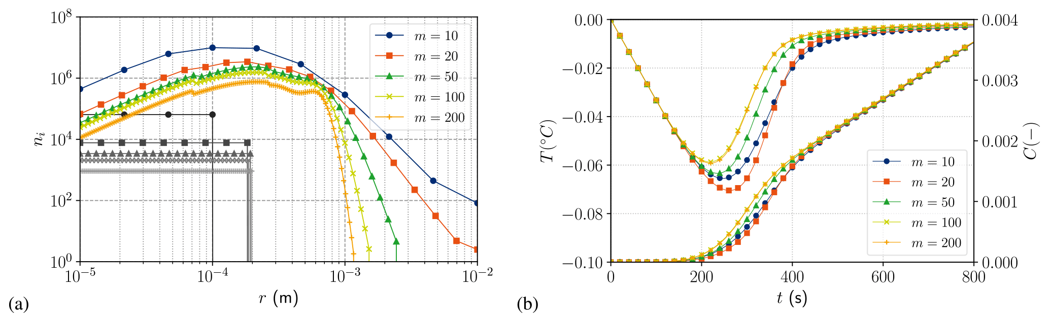
Figure 1 MSC model convergence in the number of classes with $C_{\mathrm{0}}=\mathrm{4.5}\times {\mathrm{10}}^{-\mathrm{8}}$, r₀=0.2 mm, $r_{\min }={\mathrm{10}}^{-\mathrm{5}}$ m, $r_{\max }={\mathrm{10}}^{-\mathrm{2}}$ m, dt=0.1 s, $\mathit{\varphi }=-\mathrm{1400}$ W m⁻³, $\mathit{\epsilon }=\mathrm{1.2}\times {\mathrm{10}}^{-\mathrm{3}}$ m² s⁻³, α_T=0.0876, $n_{\max }=\mathrm{8}\times {\mathrm{10}}^{\mathrm{6}}$ m⁻¹, $a_{\mathrm{f}}={\mathrm{10}}^{-\mathrm{4}}$ s⁻¹, τ_s=0 m⁻² s⁻¹ and a_d=0. Number of crystals per class (a) at initial time (black) and at time t=300 s (color). Water temperature and frazil volume fraction vs. time (b).

2.5 Study cases and model parameters

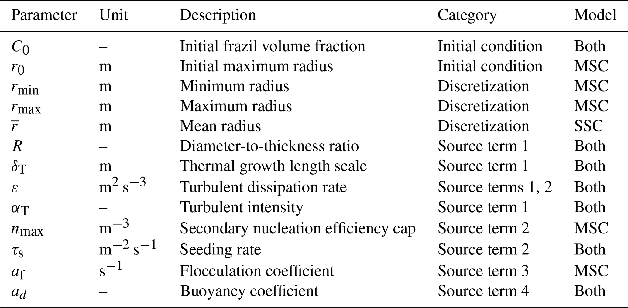
In the present study, we focus on the evolution of water temperature and total frazil volume fraction in a supercooled, well-mixed water body of depth h=1 m. To focus on the frazil modeling rather than heat budget, uncertainties deriving from exchanges with the atmosphere are neglected and the cooling rate ϕ is considered deterministic and constant over time in all experiments. Nonetheless, different values of ϕ were tested, ranging from −50 to −1000 W m⁻³, to test the variability of the results in different cooling rate situations. As described in previous sections, frazil ice models are driven by many parameters, some of which are subject to a significant degree of uncertainty. The list of parameters considered in the present study for conducting the uncertainty analysis is shown in Table 1. Some physical properties are considered constant and are taken at T=0 ^∘C such that $\mathit{\nu }=\mathrm{1.792}\times {\mathrm{10}}^{-\mathrm{6}}$ m² s⁻¹, ρ=999.82 kg m⁻³, ρ_i=916.8 kg m⁻³, $L_i=\mathrm{3.35}\times {\mathrm{10}}^{\mathrm{5}}$ J kg⁻¹, $c_p=\mathrm{4.1855}\times {\mathrm{10}}^{\mathrm{3}}$ J kg⁻¹ K⁻¹ and k_w=0.561 W m⁻¹ K⁻¹.

Table 1 Description of uncertain parameters of the frazil ice models.

Taking the SSC model as a reference, one can simply visualize the main feature of frazil dynamic systems. When time is close to zero, the initial temperature decrease rate is defined by $\underset{t\to \mathrm{0}}{lim}\dot{T}=\mathit{\varphi }/\mathit{\rho }{c}_p$. In the absence of seeding and gravitational removal (i.e., τ_s=0 and a_d=0), the temperature decreases to the maximum supercooling point, characterized by a maximal temperature depression, denoted $\mathit{\theta }=\max (T_{\mathrm{f}}-T)$, and a critical time, denoted t_c. After the maximum supercooling, the frazil production rate releases more heat compared to that released in the atmosphere, leading to an increase in water temperature which tends toward freezing point. Finally, when time tends to infinity, there is a balance between the frazil growth source term and the cooling rate. This leads to a linear increase in frazil volume fraction at a constant rate, i.e., $\underset{t\to +\mathrm{\infty }}{lim}\dot{C}=-\mathit{\varphi }/{\mathit{\rho }}_{\mathrm{i}}{L}_i$. This typical evolution of water temperature and frazil volume fraction is described in Fig. 2, in which the frazil volume fraction asymptote, denoted C^∞, is defined as

$$\begin{array}{}\text{(15)}& C^{\mathrm{\infty }}=C_{\mathrm{0}}-\mathit{\varphi }t/{\mathit{\rho }}_{\mathrm{i}}{L}_i.\end{array}$$

By introducing seeding and gravitational removal, i.e., τ_s≠0 and a_d≠0, the frazil ice long-term asymptote is modified, and we have $\underset{t\to +\mathrm{\infty }}{lim}\dot{C}=-\mathit{\varphi }/{\mathit{\rho }}_{\mathrm{i}}{L}_i+(V{\mathit{\tau }}_{\mathrm{s}}-w_r{a}_{d}C)/h$. Considering ϕ and τ_s as constant over time, this yields a convergence of the frazil volume fraction towards a finite limit, defined by the ratio between the buoyancy removal and the production rate due to thermal growth and seeding, which reads

$$\begin{array}{}\text{(16)}& C^{\mathrm{\infty }}={\displaystyle \frac{h}{a_d{w}_r}}\left(-{\displaystyle \frac{\mathit{\varphi }}{{\mathit{\rho }}_{\mathrm{i}}{L}_i}}+{\displaystyle \frac{V{\mathit{\tau }}_{\mathrm{s}}}{h}}\right).\end{array}$$

It should be observed that the steady states are not affected by the crystal growth rate. Similar observations were discussed by Rees Jones and Wells (2018) for the MSC model.

Figure 2 Typical evolution of water temperature and frazil volume fraction vs. time (a) and reproduction of Carstens (1966) case 1 experiments (b) with dt=0.1 s, $\mathit{\varphi }=-\mathrm{1400}$ W m⁻³, $\mathit{\epsilon }=\mathrm{1.2}\times {\mathrm{10}}^{-\mathrm{3}}$ m² s⁻³, α_T=0.0876, $n_{\max }=\mathrm{8}\times {\mathrm{10}}^{\mathrm{6}}$ m⁻¹, $a_{\mathrm{f}}={\mathrm{10}}^{-\mathrm{4}}$ s⁻¹, τ_s=0 m⁻² s⁻¹, a_d=0, $\stackrel{\mathrm{‾}}{r}=\mathrm{3.8}\times {\mathrm{10}}^{-\mathrm{4}}$ m, R=10, $C_{\mathrm{0}}=\mathrm{5.1}\times {\mathrm{10}}^{-\mathrm{6}}$ (SSC) and $C_{\mathrm{0}}=\mathrm{4.5}\times {\mathrm{10}}^{-\mathrm{8}}$ (MSC), r₀=0.2 m, $r_{\min }={\mathrm{10}}^{-\mathrm{5}}$ m, $r_{\max }={\mathrm{10}}^{-\mathrm{3}}$ m, m=100, and δ_T=λ.

In the following the recovery time is defined as the time when temperature has recovered 90 % of its supercooling depression. We refer to the recovery phase to describe the long-term evolution of the system, i.e., all times past recovery time. Similarly, we will refer to the transient phase as times between initial time and recovery time.

In the present study, we analyzed the uncertainty of input parameters in the main transient and steady-state features of the frazil ice models with and without gravitational removal. We started the simulation with a water temperature equal to the freezing temperature (which is supposed to be equal to zero in the absence of salinity: i.e., T_f=0 ^∘C). We checked that all the simulations ran beyond the critical time. For the range of parameters considered there, it was found that choosing a final time of t_f≃1 h was enough to capture the transient features of the ODE systems.

Note that both the SSC and MSC models are able to reproduce the experiments of Michel (1963), Carstens (1966) and Clark and Doering (2004) as shown by Svensson and Omstedt (1994) and Wang and Doering (2005). In Fig. 2 we give an example of the results of both SSC and MSC models compared to Carstens (1966) experimental results (case 1).

3 Probabilistic framework for uncertainty analysis

The objective of this section is to describe the mathematical tools necessary to study the uncertainties of SSC and MSC frazil ice models. An uncertainty study of a numerical model can be performed in three steps (Sudret, 2007). The first step consists in identifying the uncertain parameters and characterizing the probabilities of occurrence for their values through probability density functions (PDFs), which is referred to as quantification of uncertainty sources. The second step concerns the propagation of uncertainties through the interest models, generally using sampling techniques (e.g., Monte Carlo) to obtain possible values of the target outputs (here frazil ice concentration, water temperature) and compute their statistical estimates (mean, standard deviation, percentiles, etc.). The third step, called sensitivity analysis, focuses on ranking the uncertain parameters in terms of influence on the target output. In the following, formulations for the statistical estimates and sensitivity analysis indices are given, with a summary of elements essential to understand this paper. Theoretical details can be found in Soize (2017) and Sudret (2007). All uncertainty analysis computations were performed with the OpenTURNS library (version 1.18) developed by a partnership between Airbus Group, EDF R & D, IMACS, ONERA and Phimeca (Baudin et al., 2016b).

3.1 Uncertainty quantification

Let $\mathit{X}=(X^{\mathrm{1}},\mathrm{\dots },X^{n_X})$ be the vector of uncertain parameters of the frazil ice model, where n_X is the number of uncertain parameters. Let g be the interest frazil model, either SSC or MSC models presented in Eqs. (14) and (12) for temperature and Eqs. (13) and (7) for frazil volume fraction. The output of the interest models is the frazil volume fraction and water temperature discrete time series, i.e., T(t_k) and C(t_k) ($\mathrm{1}\le k\le n_t$), which we will generally denote $\mathit{Y}=(Y^{\mathrm{1}},\mathrm{\dots },Y^{n_t})$ below for the sake of simplicity. The random vectors X and Y are linked through frazil models g such that $\mathit{Y}=g(\mathit{X},\mathit{d})$, where d is a deterministic vector, i.e., fixed parameters in contrast with the uncertain set of inputs X.

To undertake the uncertainty studies, both the inputs X and the interest outputs Y are considered to be random vectors. We assume that X has a density p_X, so that $\mathbb{P}(\mathit{X}\in E\subseteq D_{\mathit{X}})=\underset{E}{\int }{p}_{\mathit{X}}\left(\mathit{x}\right)d\mathit{x}$, where E is a subset from the space of all possible values D_X. Each element Xⁱ and Y^k of the input and output vectors is hence characterized by a PDF.

The results of the uncertainty analysis are directly linked to the UQ (uncertainty quantification) study specification and consequently to the description of the uncertain input parameters X. Thus, special attention is paid to propose a relevant quantification of uncertainty sources. This particular point is addressed in Sect. 4, in which frazil literature is explored to provide adequate bounds and PDFs for each parameter identified in Table 1.

3.2 Uncertainty propagation of random variables

In the following, we suppose that PDFs of inputs X are known, in contrast to those of Y. The objective is therefore to characterize the latter by estimating statistical indicators as the PDF's mean and standard deviation. To achieve this, a Monte Carlo sampling method can be used.

In the Monte Carlo method, we generate a sample of independent observations of the random vector X using the joint PDF of the input random vector. For each observation of the input X, we evaluate the corresponding output Y. The resulting experimental design of the input random vector X is an array of size N×n_X, where each row, denoted ${\mathit{x}}_i=\left\{x^{\mathrm{1}},\mathrm{\dots },x^{n_X}\right\}$, represents a possible configuration of the frazil model. The output realizations, i.e., ${\mathit{y}}_i=\mathit{\{}{y}_i^{\mathrm{1}},\mathrm{\dots },y_i^{n_t}\mathit{\}}$, are generated by N deterministic simulations with corresponding inputs. For a sample of size N, the output of the model is a N×n_t array: $\mathit{Y}=[y_i^k{]}_{i,k}=[g^k({\mathit{x}}_i,d){]}_{i,k}\in {\mathbb{R}}^{N\times n_t}$. Each row of the matrix represents one output time series for a given set of input parameters, while each column represents the output realizations at a given time t_k.

Statistical estimators of the response can then be computed. The Monte Carlo estimation of the mean, denoted ${\widehat{\mathit{\mu }}}_{Y^k}$, and standard deviation, denoted ${\widehat{\mathit{\sigma }}}_{Y^k}$, at time t_k reads

$$\begin{array}{}\text{(17)}& {\widehat{\mathit{\mu }}}_{Y^k}={\displaystyle \frac{\mathrm{1}}{N}}\sum _{j=\mathrm{1}}^N{y}_j^k\mathrm{and}{\widehat{\mathit{\sigma }}}_{Y^k}=\sqrt{{\displaystyle \frac{\mathrm{1}}{N}}\sum _{j=\mathrm{1}}^N{\left(y_j^k-{\widehat{m}}_{Y^k}\right)}^{\mathrm{2}}}.\end{array}$$

These estimations converge to the true values following the law of large numbers (conditioned by the existence of corresponding PDF's first and second moment, i.e., expectation and variance; Soize, 2017). The convergence order of the Monte Carlo method is given by the central limit theorem, leading to a decrease in the confidence intervals' sizes proportional to $\mathrm{1}/\sqrt{N}$. In the results of this paper, confidence intervals of the estimated mean and standard deviation are computed using a bootstrap method.

3.3 Sensitivity analysis using Sobol indices

Sensitivity analysis is essential in understanding numerical models (Razavi et al., 2021). It aims at quantifying the impact of input variable imprecision on the accuracy of the model output variables. Conventional approaches to global sensitivity analysis (GSA) imply the stochastic estimation of statistical moments and indices classically achieved with the Monte Carlo technique. In the present work, the relative influence of uncertain parameters on the output time series is assessed by means of Sobol indices resulting from the ANOVA (analysis of variance) variance decomposition (Sobol, 2001). Sobol indices are computed via a modified version of the method proposed by Saltelli (2002), which is described in Appendix B. For each time step t_k ($\mathrm{1}\le k\le n_t$) and $i\in \mathit{\{}\mathrm{1},\mathrm{\dots },n_X\mathit{\}}$, first-order and total Sobol indices, denoted $S_i^k$ and $S{T}_i^k$ respectively, are computed. By definition, at any time t_k, the total Sobol sensitivity index ($S{T}_i^k$) measures the contribution to the output variance of the uncertain variable Xⁱ, including all variance caused by its interaction, of any order, with any other input variables. Thus, the variance part explained by variable interactions of the input factor Xⁱ with the other uncertain parameters is determined by subtracting the total Sobol sensitivity index ($S{T}_i^k$) and the first-order Sobol index ($S_i^k$) characterizing the influence of the variable Xⁱ alone. Finally, the discrete time first-order and total Sobol indices are aggregated, denoted AS_i and AST_i respectively, as proposed by Gamboa et al. (2014).

4 Uncertainty source quantification

Many laboratory experiments have been carried out to better understand frazil ice dynamics as summed up by Barrette (2020, 2021). These experiments, as well as field measurements, help us define parameter variability. In this section, we consider the uncertain parameters listed in Table 1 and deduce adequate variability and PDFs for uncertainty propagation and sensitivity analysis using the aforementioned data. The main geometrical properties of crystals and radial space discretization are first discussed, as well as initial concentration. We then review all the parameters involved in frazil source terms in the same chronology as presented in Sect. 2.

4.1 Crystals' geometrical properties

Description of the frazil crystals' shape has been the subject of several field and laboratory measurements (Arakawa, 1954; Daly, 1984, 1994). The crystals have been described as thin discs that grow mainly from their peripheral area. More recently, photos have brought valuable confirmation of the disc shape of frazil crystals but also highlighted the complexity in larger flocs' geometry (Clark and Doering, 2006; Ghobrial et al., 2012; McFarlane et al., 2014, 2015; Schneck et al., 2019). Let us recall that, in both SSC and MSC models, discretization is done in radial space. Therefore, either the ratio R or the thickness λ must be considered constant to fully describe disc-shaped particles. In the present study, frazil crystals are assumed to have the same aspect ratios, which is consistent with previous studies' hypotheses (Svensson and Omstedt, 1994; Holland et al., 2007). Note that Rees Jones and Wells (2018) considered constant thickness instead but highlighted a weak dependency of the thermal growth on the aspect ratio. Let us discuss the uncertainties associated with the choice of the radius discretization as well as the diameter-to-thickness ratio.

Either a mean radius or a radius space discretization must be specified for SSC and MSC models, respectively. In both cases, observed radius distribution and particle size, reported in a many studies, are taken into consideration. For the sake of synthesis, we analyzed the corresponding publications from 1950 to 2019 and report the available observations in Fig. 3. This figure is complementary to Table 7 of McFarlane et al. (2017), who summarize particle sizes from both laboratory and field measurements. Daly and Colbeck (1986) and Clark and Doering (2006) reported log-normal distributions of particles in laboratory experiments, with a mean radius ranging from 0.12 to 0.25 mm and 0.49 to 1.4 mm, respectively. This was later confirmed by Ghobrial et al. (2012) and McFarlane et al. (2015) in the University of Alberta cold room facility, with mean size ranging from 0.66 to 0.94 mm. Schneck et al. (2019) recently published similar results under different salinities, with mean radius ranging from 0.45 to 0.52 mm. Log-normal distributions were also observed in field studies, with the mean ranging from 0.59 to 0.94 mm in a report by McFarlane et al. (2017). Gathering together all reported mean radius ranges, an uncertainty interval of $\mathrm{1.2}\times {\mathrm{10}}^{-\mathrm{4}}$ to $\mathrm{2.1}\times {\mathrm{10}}^{-\mathrm{3}}$ m was chosen for the mean radius in the SSC model. When their full variation range is considered, frazil crystal sizes are known to follow a log-normal distribution as previously argued, but there is no evidence or reason for the mean radius being log-normal as well. The number of field and laboratory observations is still too small to fit an empirical PDF on the mean radius with reasonable confidence. Hence, a log-uniform PDF is chosen with the previously described bounds. Using log-uniform approximate distributions allows us to explore by means of evenly distributed values the parameters that vary over several orders of magnitude.

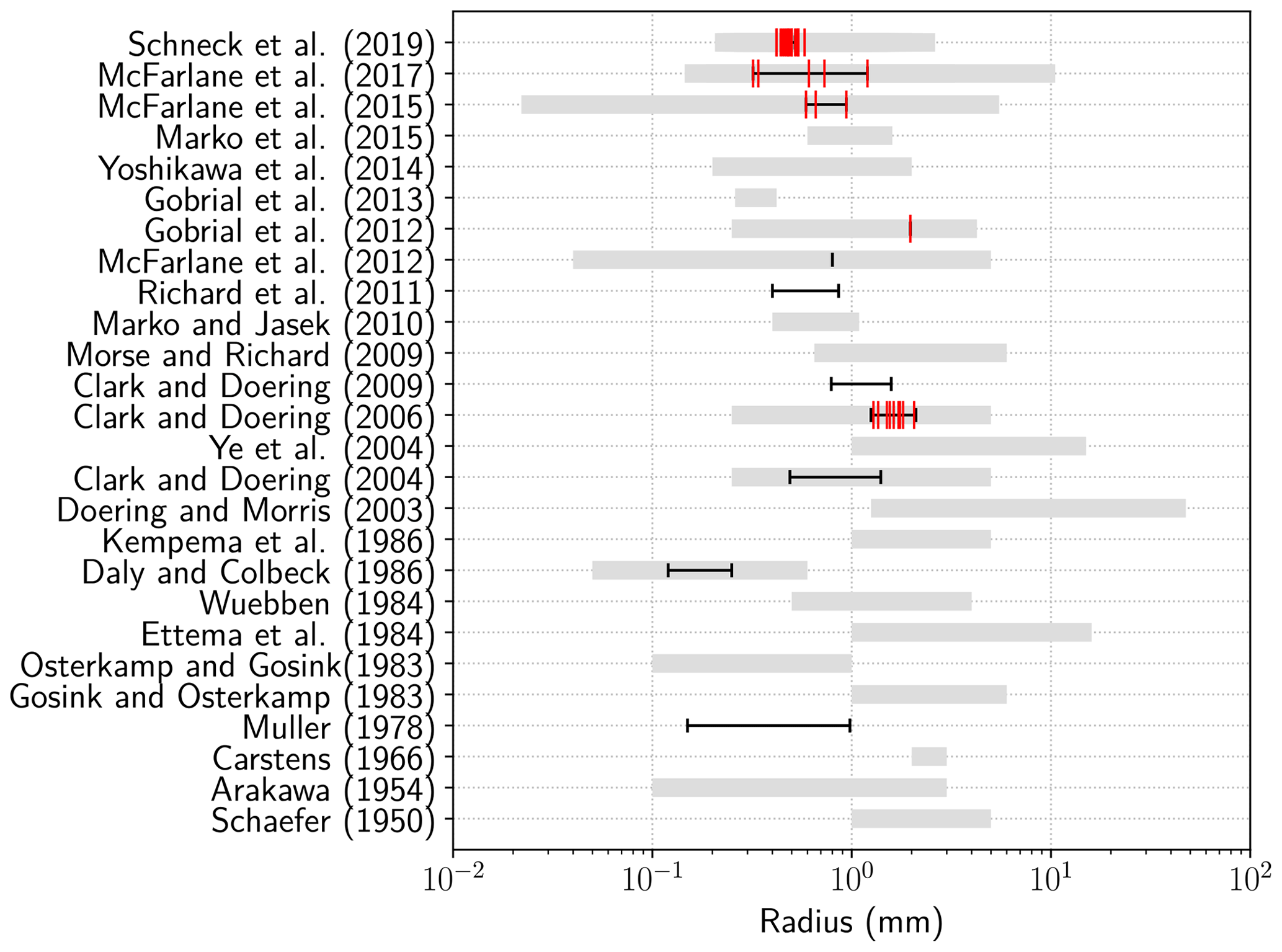
Figure 3 Particle-size ranges (thick grey line), mean range (thin dark line) and log-normal distributions' mean radius (red vertical ticks) reported in field or laboratory experiments (Schaefer, 1950; Arakawa, 1954; Carstens, 1966; Gosink and Osterkamp, 1983; Osterkamp and Gosink, 1983b; Ettema et al., 1984; Wuebben, 1984; Kempema et al., 1986; Daly and Colbeck, 1986; Doering and Morris, 2003; Ye et al., 2004; Ye and Doering, 2004; Clark and Doering, 2004, 2006, 2009; Marko and Jasek, 2010; Ghobrial et al., 2012; McFarlane et al., 2012; Ghobrial et al., 2013; McFarlane et al., 2015; Kempema and Ettema, 2016; McFarlane et al., 2016, 2017; Schneck et al., 2019).

For the MSC model, both a minimum and a maximum radius are to be determined for the bounds of the radial discretization. The minimum radius can be determined from Lal et al. (1969) survival theory and is about 4 µm (Mercier, 1984). The maximum size of frazil particles is about 1 to 5 mm according to Clark and Doering (2004), but frazil flocs can be significantly larger as shown by Schneck et al. (2019) and can range up to several centimeters (McFarlane et al., 2017). Svensson and Omstedt (1994) worked with [$\mathrm{4}\times {\mathrm{10}}^{-\mathrm{6}}$, $\mathrm{3}\times {\mathrm{10}}^{-\mathrm{3}}$] m while Wang and Doering (2005) and Rees Jones and Wells (2018) chose [$\mathrm{7}\times {\mathrm{10}}^{-\mathrm{5}}$, $\mathrm{5}\times {\mathrm{10}}^{-\mathrm{3}}]$ m and [$\mathrm{5}\times {\mathrm{10}}^{-\mathrm{5}}$, $\mathrm{5}\times {\mathrm{10}}^{-\mathrm{2}}$] m, respectively. In the literature, r_min is taken to be between 10⁻⁶ and 10⁻⁴, so we chose an intermediate order of magnitude of $r_{\min }={\mathrm{10}}^{-\mathrm{5}}$ m. The same choice was made for the maximum radius, leading to a value of $r_{\max }={\mathrm{10}}^{-\mathrm{3}}$ m. Both parameters were then considered as uncertain parameters with log-uniform PDFs and were taken to be within [10⁻⁶, 10⁻⁴] for r_min and within [10⁻³, 10⁻¹] for r_max.

The aspect ratio ranged from 6 to 13 in the study by Daly and Colbeck (1986), while there were greater values, from 12.2 to 16.33, in Clark and Doering (2004, 2006). Arakawa (1954) reported an even wider aspect ratio range, from 5 to 100. More recently, McFarlane et al. (2014) reported aspect ratios ranging from 11 to 71 with a mean of 37 and a standard deviation of 11. Considering all these observations, an uncertainty range of 5 to 100 was chosen for the diameter-to-thickness ratio. As not enough data to properly fit a PDF on aspect ratios were provided, a uniform PDF is chosen for the sensibility analysis (maximum entropy principle; Soize, 2017).

Weak dependency of the thickness on the radius was reported by McFarlane et al. (2014), who suggest assuming a increasing aspect ratio as discs grow instead of a constant aspect ratio. Note also that, as frazil ice forms larger flocs, the disc shape hypothesis commonly accepted in models does not hold anymore. This could lead to erroneous estimations of the thermal growth rate of larger flocs. However, neither the variability of the aspect ratio in the crystals' distribution nor that of the shape is considered in the present study, and we make the assumption that r and R are independent.

4.2 Initial concentration

As previously mentioned, either a non-zero initial volume fraction or a non-zero seeding rate is required to trigger thermal growth in the model. In experimental facilities, frazil ice nuclei are sometimes artificially introduced in water to initiate frazil ice growth (Muller, 1978; Tsang and Hanley, 1985), but the initial concentration is rarely addressed and depends on the method of initial seeding. As such, a large uncertainty domain is considered in this study for the initial volume fraction of frazil, ranging from 10⁻⁸ to 10⁻⁴, to account for the lack of data on this parameter. Additionally, a log-uniform PDF is retained since the parameter range variation varies over several orders of magnitude.

For the MSC model, it is necessary to choose how the initial volume fraction is distributed over size classes. One possibility is to initialize the system with log-uniform distributions, similar to the one observed in laboratory experiments. However, observations of nuclei close to r_c in size are limited. Consequently, authors have preferred simpler initialization methods, whereby a constant number of crystals is distributed equally over all classes (Svensson and Omstedt, 1994; Wang and Doering, 2005; Rees Jones and Wells, 2018). Holland et al. (2007) argued that distributing the initial volume fraction over a range of radii, thus changing the initial number of particles per class, significantly impacts results. They found that filling only the first size class, as in Hammar and Shen (1995), has less impact on results and should therefore be the preferred initialization method. Given poor evidence of initial predominance of each class in nature, we decided to test both initialization methods, i.e., distributing the initial volume fraction over a range of small radii as presented in Sect. 2.4 and then feeding only the first class as suggested by Holland et al. (2007). For the first method, ice nuclei are supposed to be initially spread between the minimum radius r_min and a threshold radius r₀, which we suppose can only be smaller than the mean radius (see Fig. 3). Therefore, the threshold r₀ is considered uncertain within the bounds [$\mathrm{1.2}\times {\mathrm{10}}^{-\mathrm{4}}$, $\mathrm{2.1}\times {\mathrm{10}}^{-\mathrm{3}}$]. For the second method, we set r₀=r_min, so that only the first receives the initial concentration.

4.3 Thermal growth and turbulent parameters

As shown in Eq. (2), thermal growth (1) is mainly affected by two uncertain parameters, which are the Nusselt number and the thermal boundary layer thickness. In this section, we discuss the uncertainty of both parameters. Since the Nusselt number is being modeled via turbulent parameters, namely the turbulent dissipation rate and the turbulent intensity, their uncertainty is also addressed.

As discussed by Rees Jones and Wells (2018), the thermal boundary layer thickness δ_T is not constant around a crystal, and in recent studies there has been an inconsistent scaling of thermal growth. Svensson and Omstedt (1994) chose the length scale as δ_T=λ, while others have chosen δ_T=r (Smedsrud and Jenkins, 2004; Holland et al., 2007), leading to a serious underestimation of the growth rate, since λ<r for frazil discs. Rees Jones and Wells (2015) have shown that there is a logarithmic dependency of the thermal growth on the aspect ratio that favors the δ_T=λ scaling. To account for the variability of the thermal boundary layer thickness, δ_T should be taken as an uncertain parameter. However, it should be mentioned that, with the variation range being ${\mathit{\delta }}_{\mathrm{T}}\in [\mathit{\lambda },r]$, the ANOVA methodology (Sect. 3.3) cannot be applied, since the set of uncertain inputs, which contains δ_T and $\mathit{\lambda }/r$, cannot be considered independent anymore. To overcome this difficulty, the sensitivity analysis is conducted with the most appropriate scaling: i.e., δ_T=λ, for both the SSC and MSC models. Nevertheless, we propose to investigate the impact of scaling by considering ${\mathit{\delta }}_{\mathrm{T}}\in \left[\min \right(\mathit{\lambda }),\max (r\left)\right]$ to avoid modeling dependency. A log-uniform PDF is used, and min(λ) and max(r) are estimated from their full variation ranges. A third experiment was also carried out with the δ_T=r scaling. The three results are then compared for the SSC model.

Two main turbulence parameters are considered: turbulent dissipation rate ε and turbulent intensity α_T, both impacting the Nusselt number (see Eqs. 3 and 4). For rivers, the dissipation rate can be estimated using friction velocity $u_{*}=\sqrt{g{R}_{\mathrm{h}}S}$ such that

$$\begin{array}{}\text{(18)}& \mathit{\epsilon }={\displaystyle \frac{u_{*}^{\mathrm{3}}}{\mathit{\kappa }{R}_{\mathrm{h}}}}\left[\ln \left({\displaystyle \frac{u_{*}{R}_{\mathrm{h}}}{\mathit{\nu }}}\right)-\mathrm{1}\right],\end{array}$$

where g is gravity, R_h the hydraulic radius, S the slope of the river, κ the von Karman constant (generally taken as equal to 0.4) and ν the viscosity of water. Daly (1994) summarized the dissipation rate for several experiments (Michel, 1963; Carstens, 1966; Tsang and Hanley, 1985; Muller, 1978) using Eq. (18) and found values ranging from $\mathrm{7}\times {\mathrm{10}}^{-\mathrm{5}}$ to 0.4667 m² s⁻³. A similar method was described by McFarlane et al. (2015) to estimate the dissipation rate in rivers, leading to values ranging from $\mathrm{4.2}\times {\mathrm{10}}^{-\mathrm{4}}$ to 1.4968 m² s⁻³. Schneck et al. (2019) summarized dissipation rates observed in oceans, ranging from 10⁻⁹ to 10⁻² m² s⁻³ and from 10⁻¹⁰ to 10⁻³ m² s⁻³ in polar regions. In the present study, we consider dissipation rates varying between 10⁻⁹ and 1.5 m² s⁻³, which cover most flows encountered in rivers and oceans. Similarly, we consider a wide range of flows from low turbulence to high turbulence intensity which include most of the work presented in Fig. 3, leading to a turbulence intensity ranging from 1 % to 20 %. Log-uniform PDFs are considered for both the dissipation rate and the turbulent intensity. Note that turbulence influences not only the rate of growth of frazil crystals but also the rate of secondary nucleation, thus impacting the frazil size distribution.

4.4 Other source terms

Following the same order as in Eq. (1), let us discuss uncertain parameters involved in frazil source terms other than thermal growth: secondary nucleation (2), flocculation (3) and gravitational removal (4). It should be mentioned that almost no direct observations of these processes have been reported in the literature. Therefore, the definition of the uncertainty intervals is mainly based on expert knowledge and past numerical experiments in which parameters were determined by comparison to observed radius distributions.

• The uncertainty interval of the seeding rate is set after Daly (1994) to [$\mathrm{3}\times {\mathrm{10}}^{-\mathrm{1}}$, 10⁻⁴] m⁻² s⁻¹, and to simplify the uncertainty analysis, it is considered constant over time. For the secondary nucleation, Svensson and Omstedt (1994) proposed setting a common value for n_max that would allow a focus on calibration of the initial seeding. They found that a value of $n_{\max }=\mathrm{4}\times {\mathrm{10}}^{\mathrm{6}}$, along with initial seeding of the order of magnitude of n₀=10⁴, gave satisfactory results compared to the experimental results of Michel (1963) and Carstens (1966). Wang and Doering (2005) found that fitting a single n_max value for all experiments was unsatisfactory. Instead, they proposed fitting both the initial seeding and n_max, leading to values ranging from 2×10⁴ to 2×10⁵ for Clark and Doering (2004) experiments and from 2×10⁴ to 2×10⁵ for Carstens (1966) experiments. Smedsrud (2002) proposed a different value of n_max=10³, which was also used by Smedsrud and Jenkins (2004) and Holland and Feltham (2005).

• Similarly, the flocculation parameter a_f was calibrated to a value of 10⁻⁴ s⁻¹ by Svensson and Omstedt (1994), who compared the results of their simulation to the expected size distribution spectra (other parameters in their model, like the number of class, the heat sink, the turbulent dissipation rate and initial condition were set to m=20, $\mathit{\varphi }=-\mathrm{1000}$ W m⁻³, $\mathit{\epsilon }={\mathrm{10}}^{-\mathrm{3}}$ m² s⁻³ and n_i(t₀)=10⁴ ($\mathrm{1}\le i\le m$)). From all previous calibration studies, one could choose n_max from 10³ to 10⁷ and $a_{\mathrm{f}}={\mathrm{10}}^{-\mathrm{4}}$. But given the fact that secondary nucleation and flocculation are still very poorly understood and modeled, we choose large uncertainty intervals for these parameters. We added an order of magnitude for the bounds leading to n_max ranging from 10² to 10⁸, and we suppose that flocculation can, depending on the conditions, be negligible, so that a_f varied from 10⁻⁸ to 0⁻³. The parameters n_max and a_f are considered independent from hydrodynamic parameters, and log-uniform PDFs were chosen for both.

• The gravitational removal is affected by both the buoyant rise velocity of frazil particles and deposition process once particles reach the surface of the water column. Several attempts to measure the frazil rise velocity were made (Osterkamp and Gosink, 1983a; Wuebben, 1984; McFarlane et al., 2014), and many formulations were proposed as summarized by McFarlane et al. (2014). Significant scatter can be observed in the data as shown on Fig. 10 of McFarlane et al. (2014), with velocities ranging from approximately 0.7 to 16 mm s⁻¹ for a radius of 1 mm. Models exhibit significant differences as well (see Fig. 4). To take into account uncertainties inherent to the choice of the rise velocity model, a buoyancy parameter a_d is introduced. A rise velocity envelope, combining the results of all models, can be defined by upper and lower bounds denoted w_max(r,R) and w_min(r,R) (see Fig. 4). The interval of a_d is defined from the mean of the gap between the simplified formulation used in the present study for w_r (Svensson and Omstedt, 1994) and upper and lower bounds of the rise velocity envelope. To avoid the modeling of dependencies, a constant value is taken for a_d, even if the envelope depends on the radius and on the diameter-to-thickness ratio. Finally, we propose $a_d\in [a^{-},a^{+}]$, in which $a^{+}=\mathrm{mean}\left(w_{\max }\right(r,R)/w_r(r\left)\right)$ and $a^{-}=\mathrm{mean}\left(w_{\min }\right(r,R)/w_r(r\left)\right)$. By considering $r\in [{\mathrm{10}}^{-\mathrm{5}},{\mathrm{10}}^{-\mathrm{2}}]$ m and $R\in [\mathrm{5},\mathrm{100}]$, the following interval is obtained: $a_d\in [\mathrm{0.086},\mathrm{1.51}]$. Finally, it should be noted that this uncertainty quantification is rather imprecise since the rise velocity dispersion depends on the shape of the particles and flow conditions. Therefore, our analysis could be refined by taking into account dependencies. Also note that low values of a_d could also be justified from the uncertainty of the deposition process, which is not modeled in the present study.

Figure 4 Comparison of frazil rise velocity models with R=10 (a) and the rise velocity envelope chosen for the uncertainty analysis (b) (Zacharov et al., 1972; Gosink and Osterkamp, 1983; Ashton, 1983; Wuebben, 1984; Daly, 1984; Svensson and Omstedt, 1994; Matoušek, 1992; Shen and Wang, 1995; Morse and Richard, 2009).

4.5 Summary of uncertain parameters

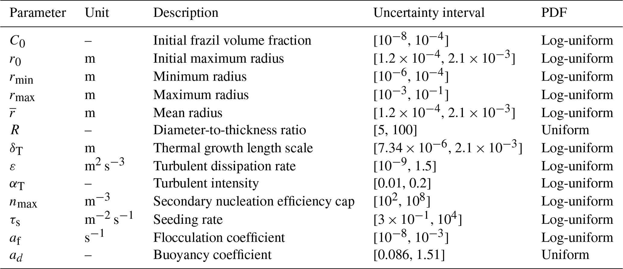
To conclude the uncertainty quantification, all the uncertain parameters, their bounds and PDFs are summarized in Table 2.

Table 2 Uncertain parameters of the frazil ice models and their PDFs.

5 Uncertainty propagation and sensitivity analysis

In this section, we present the different Monte Carlo simulation cases considered for the uncertainty analysis, as synthesized in Table 3. Then we discuss the results of the uncertainty propagation and the sensitivity analysis obtained for both SSC and MSC models.

5.1 Propagation cases

Monte Carlo simulations are first carried out without seeding and gravitational removal (τ_s=0 and a_d=0) for both SSC and MSC models, which correspond to cases 1 and 2, respectively. Seeding and gravitational removal processes are subsequently considered in cases 3 and 4. For each case, the set of uncertain parameters is described in Table 2. When not in X, parameters are considered deterministic with the following default values: a_d=0, τ_s=0 m² s⁻¹, δ_T=e, $r_{\min }={\mathrm{10}}^{-\mathrm{5}}$ m and $r_{\max }={\mathrm{10}}^{-\mathrm{3}}$ m.

Table 3 List of Monte Carlo simulations and their associated input random vectors X, sampling size and number of function calls. Seeding rate and buoyancy velocity are set to τ_s=0 and a_d=0 in cases 1 and 2.

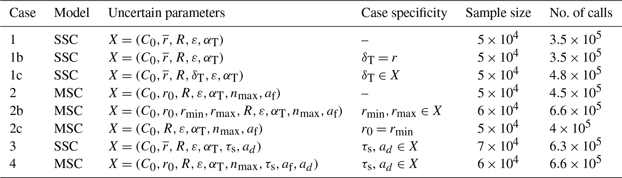
Additional Monte Carlo simulations were carried out to examine the influence of specific parameters. For example, although δ_T=e is the preferred scaling and is chosen by default in all experiments, we also tested δ_T=r and ${\mathit{\delta }}_{\mathrm{T}}\in [e,r]$ in experiments 1b and 1c to investigate the impact on results. In experiments 2b and 2c, modifications of the MSC model uncertain parameters are also taken into account, in order to investigate the impact of the radius bounds r_min and r_max, as well as the alternate methods of initialization discussed in Sect. 4.2.

Statistical estimators are evaluated every 10 s of physical time, leading to n_t=400. To cope with the computational cost of multi-class experiments, we used clusters to run all simulations in parallel. The computation time of 4.5×10⁵ multi-class simulations with m=100 is ∼24 h with 960 processes. A total of 4 million simulations were carried out for uncertainty propagation.

5.2 Results without gravitational removal

By neglecting the seeding rate and gravitational removal source terms, the steady state corresponds to the constant frazil production rate that only depends on the heat sink ϕ, as shown in Sect. 2.5. As expected, the statistical estimator time series for temperature and frazil volume fraction, presented in Fig. 5 for cases 1 and 2, show a very narrow scatter of the output PDF at the start of simulation and at steady state. The results converge towards the two asymptotes (T⁰ and C^∞ respectively) of the mono-class ODE system: i.e., the constant cooling rate when t→0 (initial supercooling phase) and the constant frazil production rate when t→∞ (recovery phase). However, for both SSC and MSC models, the transition between the two asymptotes of the ODE system is spread out, and there is a significant difference in maximum supercooling between the 5th, 25th, 75th and 95th percentiles. For the median, a maximum supercooling of $T\left(t_{\mathrm{c}}\right)\simeq -\mathrm{0.018}$ ^∘C is reached at t_c=180 s for the SSC model. The gap between the 5^th and 95^th percentile maximum supercooling is Δt_c=890 s and Δθ=0.097 ^∘C. Note that the envelope obtained with the standard deviation gives a poor description of the output since its PDF is not normal, as it can be seen from the $\widehat{\mathit{\mu }}\pm \widehat{\mathit{\sigma }}$ lines in the Fig. 5.

Figure 5 Uncertainty propagation results for SSC (case 1) for temperature (a) and frazil (c) and MSC (case 2) for temperature (b) and frazil (d): mean, standard deviation, median, and the 5th, 25th, 75th and 95th percentiles are computed for t_k ($\mathrm{0}\le k\le n_t$).

Similar results were obtained with the MSC model, which recovers the same asymptote at steady state; however, there is a slight residual scatter at recovery. For case 2, we observed slightly less scatter at the maximum supercooling than with the SSC model, and the gap between the 5th and 95th percentile maximum supercooling was Δt_c=820 s and Δθ=0.08 ^∘C.

Time series of the first-order Sobol indices are presented in Fig. 6 (see Appendices E and F for details). In Appendix C, we also present the first- and total-order Sobol indices at times t_c, 2×t_c and t_f with 95 % confidence intervals, as well as the aggregated Sobol indices, computed via Eq. (B7). The time evolution of Sobol indices of temperature and frazil was similar for both the SSC and MSC with the exception of the initial concentration, which, as expected, had more of an impact on frazil volume fraction at the start of simulation.

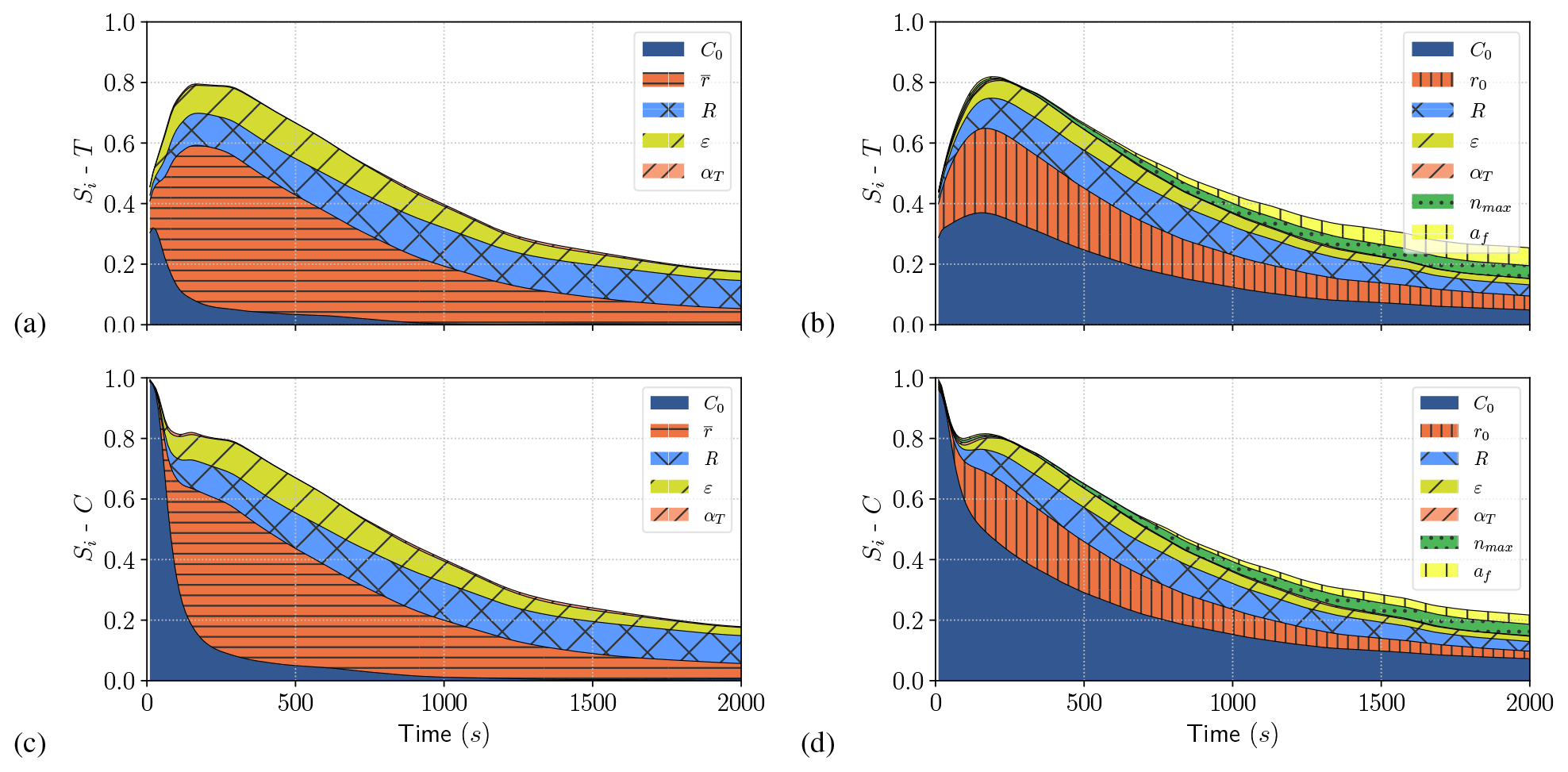
Figure 6 Time series of first-order Sobol indices (S_i) for SSC (case 1) for temperature (a) and frazil (b) and MSC (case 2) for temperature (b) and frazil (d).

For the SSC model, the initial concentration plays an important role at the start of the simulation. However, its influence quickly decreases, and the most influential parameter becomes the radius, with a peak influence reached at the median value of the time of maximum supercooling. Thus, using the average radius as the calibration parameter of the SSC model seems to be the most relevant choice. The most influential parameters after radius are the diameter-to-thickness ratio and dissipation rate of turbulent kinetic energy. In experiments, the turbulent dissipation rate is often better known than the initial concentration or crystal shape. In natural water bodies, turbulent dissipation rate measurements are rare but turbulence models can be use to estimate these parameters. Therefore, one could then choose the initial frazil volume fraction or diameter-to-thickness ratio as a secondary calibration parameters.

For the MSC model, the most influential parameters prior to maximum supercooling are initial concentration (C₀) and maximum initial radius (r₀), with both control the initial distribution (and consequently the initial condition of the system). Using these initial distribution parameters to calibrate the transient phase until maximum supercooling seems to be the right approach. However, specifying a more accurate initial distribution (not necessarily uniform) by comparison with what can be observed in nature would be a welcome improvement, although this requires further research.

At the recovery, the parameters of secondary nucleation and flocculation processes (n_max and a_f), both impacting steady-state crystal distribution, become more influential. However, the hierarchy of parameters is less obvious than for the SSC model. In addition, we observed strong interactions between parameters when the model reaches steady state (see blank space on Fig. 6 and total Sobol indices in Appendix F), which might lead to difficulties in the calibration process. Aggregated Sobol indices summarized in Fig. 7 confirm the relative influence of each parameter over the whole duration of the simulation, taking into account both the transient phase and steady state.

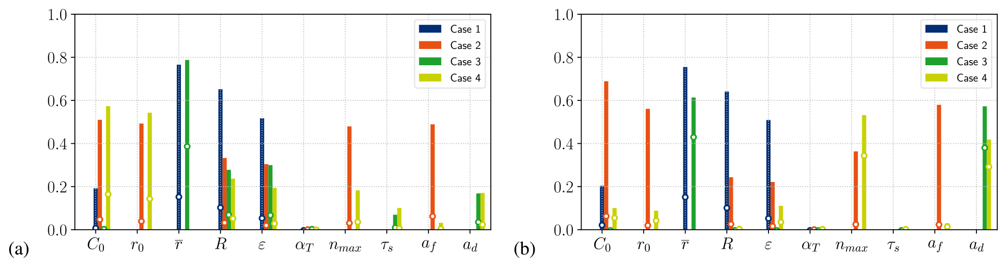
Figure 7 Aggregated first-order Sobol indices (dots) and aggregated total Sobol indices (bars) for temperature (a) and total frazil volume fraction (b) for cases 1, 2, 3 and 4.

While the approach adopted by Svensson and Omstedt (1994) – i.e., tweaking the values of n_max and a_f – was adequate to calibrate the frazil distribution in MSC models, the present sensitivity analysis shows that it might not be the best option to calibrate water temperature and frazil total volume fraction. Results suggests that more focus should be on the initial condition to calibrate supercooling, by modifying initial seeding like it was done by Wang and Doering (2005) or by modifying the initial distribution itself. We therefore suggest calibrating the supercooling curve with the help of the initial distribution, along with secondary nucleation and flocculation parameters to calibrate the evolution of size distribution over time. Hopefully, recent observations of the transient evolution of frazil size distribution (McFarlane et al., 2015; Schneck et al., 2019) will provide the necessary data to carry out an optimal calibration of the identified parameters.

5.3 Influence of gravitational removal and seeding

Long-term evolution that does not take account of gravitational removal leads to infinite increase in frazil concentration as long as the cooling rate remains constant (see Eq. 15). This asymptotic behavior of the models has never been observed in experiment or in nature. Clark and Doering (2006) observed a peak in the number of particles per image they recorded, located shortly after maximum supercooling, after which there was a small decrease in the number of particles and a stagnation at residual supercooling. Similar observations were also reported by McFarlane et al. (2015) and Schneck et al. (2019). The models in which only thermal growth is considered do not incorporate the required physics to properly reproduce what is observed. However by introducing gravitational removal, as shown in Sect. 2.5, the models converge towards a constant frazil volume fraction (see Eq. 16). In this section we analyze the results of the uncertainty propagation and sensitivity analysis for cases 3 and 4, which include the seeding rate and gravitational removal source terms.

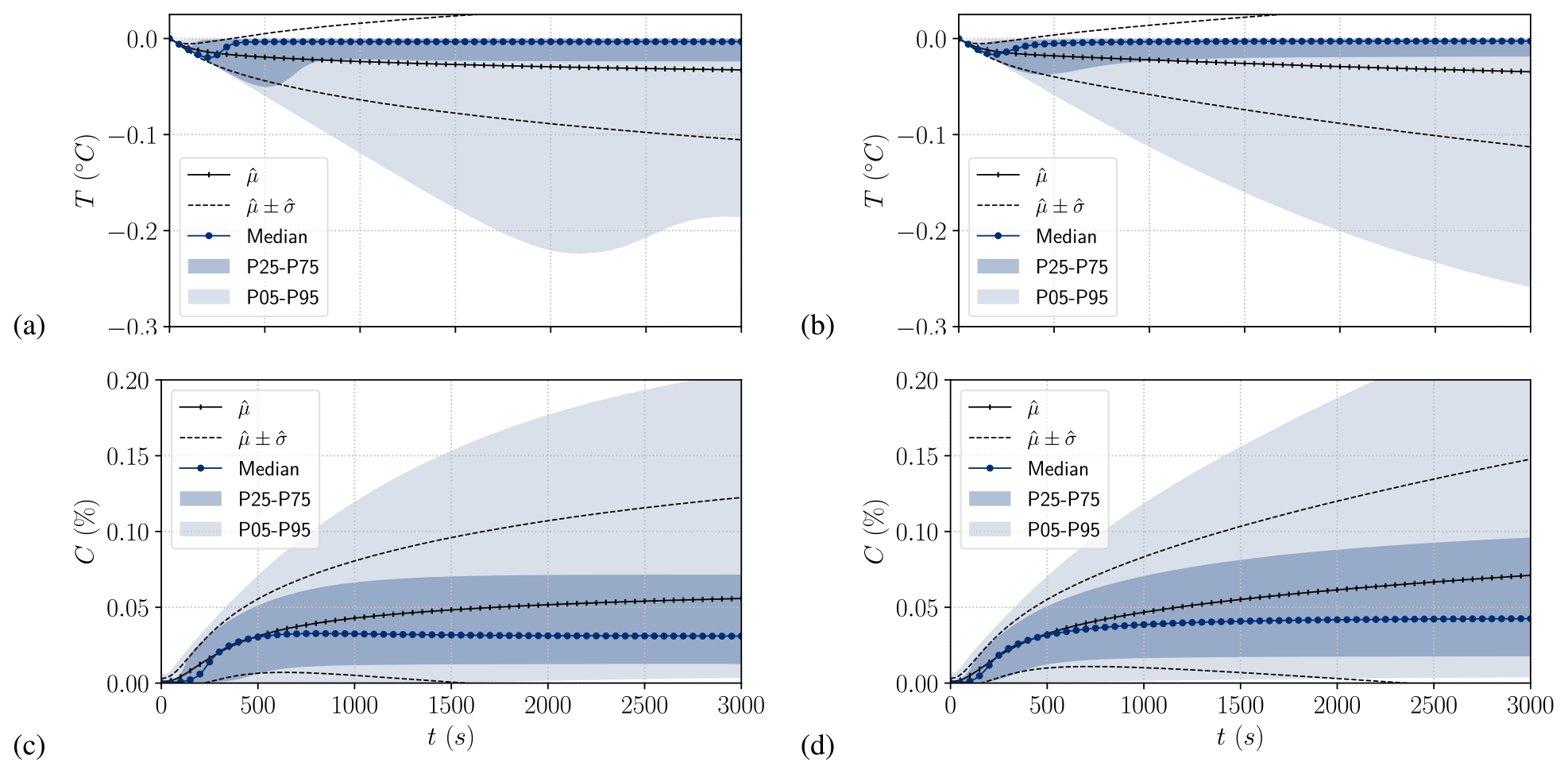
Figure 8 Uncertainty propagation results for SSC (case 3) for temperature (a) and frazil (c) and MSC (case 4) for temperature (b) and frazil (d): mean, standard deviation, median, and the 5th, 25th, 75th and 95th percentiles computed for t_k ($\mathrm{0}\le k\le n_t$).

At steady state, the introduction of gravitational removal leads to wide scatter of both temperature and frazil as shown by the comparison of Figs. 8 and 5 (see Appendices G and H for details). This is caused by the variation of the steady-state frazil volume fraction, which depends on the heat flux ϕ and model parameters inherent in secondary nucleation, flocculation and rise velocity (n_max, a_f and a_d). Significant supercooling values are observed as the water temperature (5th percentile) drops below −0.2 ^∘C, which is really low compared to what can be observed in rivers. This is due to the highest values of the buoyancy velocity combined with low thermal growth rate. High gravitational removal withdraws a large amount of the frazil volume fraction from the water and thus limits the amount of latent heat release to water that would increase its temperature. No significant difference is observed in the output scatter between SSC and MSC models similarly to cases 1 and 2. However, minimum supercooling is not reached on the 5th percentile with the MSC as opposed to the SSC model. This is due to the dependency of the buoyancy velocity on the radius, which is not constant in the MSC model as opposed to the SSC model. This also causes the median frazil volume fraction at steady state to be slightly different in the two models.

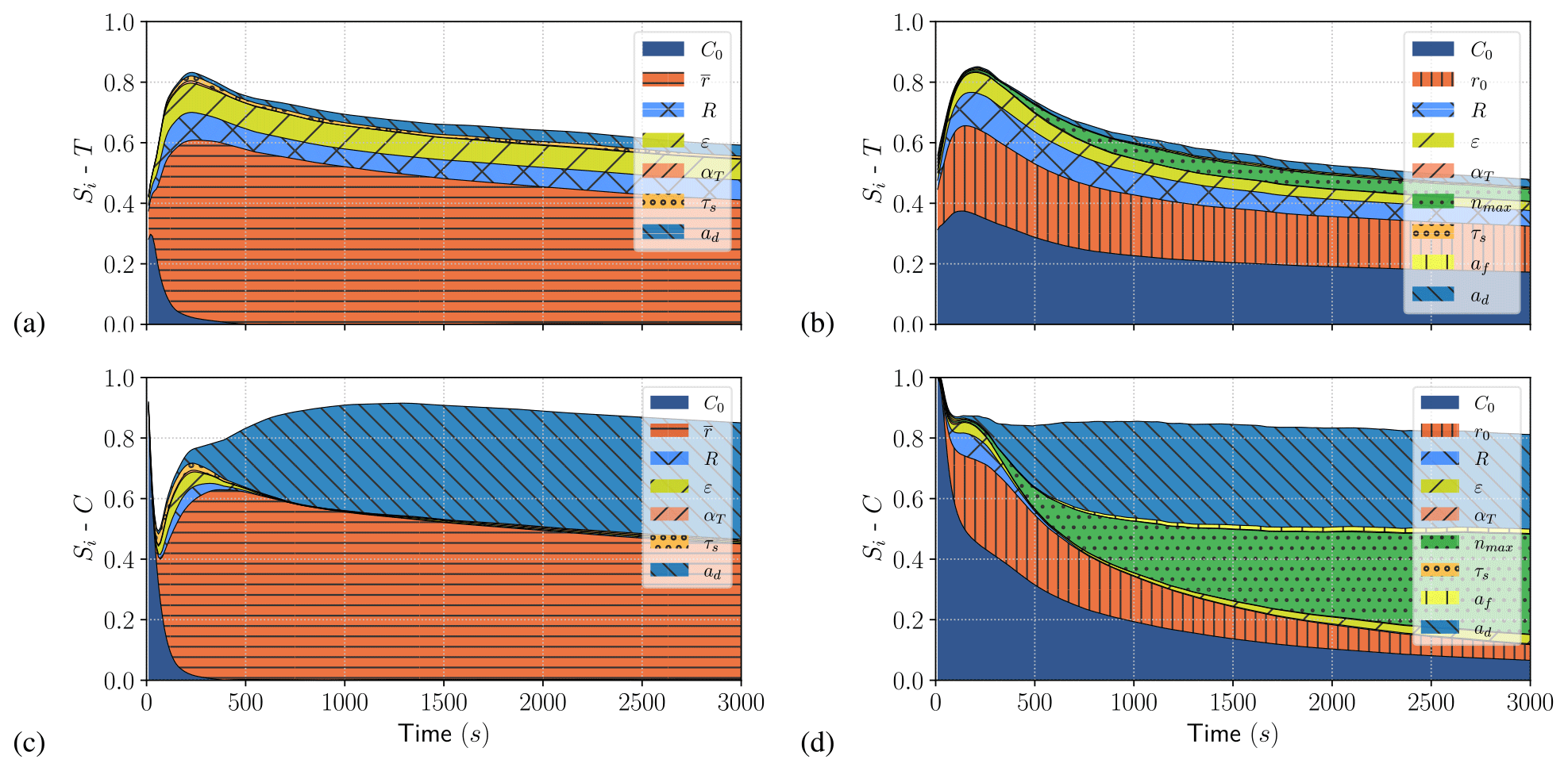
Figure 9 Time series of first-order Sobol indices (S_i) for SSC (case 3) for temperature (a) and frazil (c) and MSC (case 4) for temperature (b) and frazil (d).

With the SSC model at recovery, the first-order Sobol indices on frazil volume fraction (S_i−C) in Fig. 9 show a major influence of the radius and the buoyancy coefficient ($S_{\stackrel{\mathrm{‾}}{r}}=\mathrm{0.381}$ and $S_{a_d}=\mathrm{0.382}$, respectively at t=t_f), the main parameters influencing the gravitational removal (see Eq. 15). For the MSC model, the most influential parameters at recovery are n_max and a_d ($S_{n_{\max }}=\mathrm{0.37}$ and $S_{a_d}=\mathrm{0.26}$, respectively at t=t_f), which is consistent with Eqs. (27) and (29) of Rees Jones and Wells (2018). The hierarchy of the most influential parameters is similar to cases 1 and 2 prior to maximum supercooling. However accurate modeling of the buoyancy velocity of frazil crystals is essential, as it has a very important influence on the long-term evolution of the system, and therefore merits particular attention.

5.4 Maximum supercooling scatter

The results discussed above were obtained with a cooling rate of −500 W m⁻³. Several cooling rates, ranging from −50 to −1000 W m⁻³, were tested with case (1) to assess variations in maximum supercooling predictions. We found that the higher the cooling rate, the greater the scatter of the predicted maximum supercooling temperature, as presented in Figs. 10 and 11. This is the opposite for the time until maximum supercooling peak, where the higher the cooling rate, the lower the scatter in supercooling time. These results conform to observations of Carstens (1966) and Ye et al. (2004) that the degree of supercooling increases with the heat sink rate while the time to supercooling decreases. Note that the gap between the 5th and 95th percentile maximum supercooling predictions is as much as Δt_c=2540 s with $\mathit{\varphi }=-\mathrm{50}$ W m⁻³ and Δθ=0.142 ^∘C with $\mathit{\varphi }=-\mathrm{1000}$ W m⁻³ as shown in Fig. 11. The dispersion both in time to supercooling and degree of supercooling is significant. This shows the importance of having a good quantification of input parameters to be able to predict the maximum supercooling point.

Figure 10 Maximum supercooling point scatter computed from median and 5th, 25th, 75th and 95th percentile time series at different cooling rates ($\mathit{\varphi }=-\mathrm{50}$, −100, −250, −500 and −1000 W m⁻³) for case 1 and with $\mathit{\varphi }=-\mathrm{500}$ W m⁻³ for case 2. Global view (a) and focus on initial time (b).

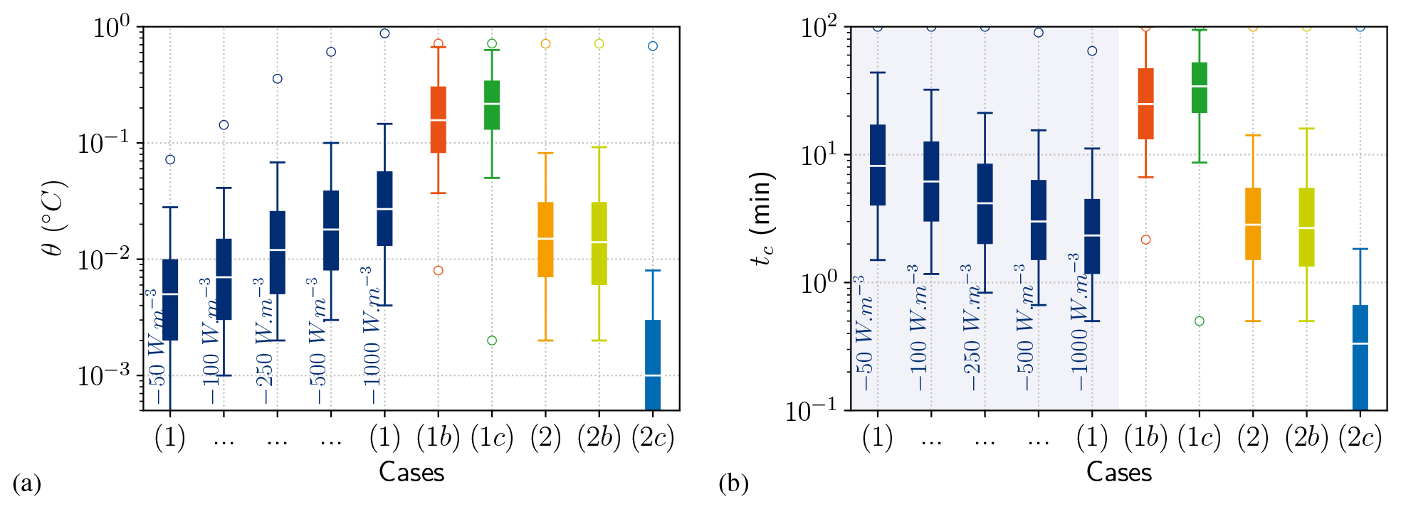
Figure 11 Maximum supercooling point scatter computed from median and 5th, 25th, 75th and 95th percentile time series at different cooling rates (−50, −100, −250, −500 and −1000 W m⁻³) for case 1; comparison between the choice of the length scale δ_T (cases 1b and 1c); and comparison between different initial conditions (cases 2b and 2c) with $\mathit{\varphi }=-\mathrm{500}$ W m⁻³. Maximum degree of supercooling (a) and maximum supercooling time (b). The white line is the median, the wide box is delimited by the 25th and 75th percentiles, the thin line is delimited by the 5th and 95th percentiles, and the round dots corresponds to minimum and maximum values.

Results obtained from different scalings of the thermal boundary layer are also shown in Fig. 11. A significant increase in scatter is observed for the δ_T=r compared to δ_T=λ scaling, consistent with the fact that thermal growth is clearly underestimated (Rees Jones and Wells, 2018). With δ_T taken as an uncertain parameter with a log-uniform PDF within the bounds [min(λ), min(r)], the result is also more widely scattered by the same order of magnitude as with δ_T=r. The results highlight the significant influence of the choice of scaling for the boundary layer. Choice of scaling also explains inconsistencies in calibrated parameters in the literature.

Finally, let us discuss the results obtained with the MSC model, which need to be viewed from the standpoint of the way it is initialized. By taking the minimum and maximum radius as uncertain parameters (case 2b), we observe an increased gap between the 5th and 95th percentiles, and we have Δt_c=930 s and Δθ=0.09 ^∘C (see Fig. 11). The constant feed of first-class nuclei due to secondary nucleation accentuates the influence of the minimum radius parameter. This explains why the minimum radius has more influence on the results than the maximum radius as shown in Appendix D. Additionally, the volume growth rate being higher for small classes makes the initial distribution of concentration a determining choice. The more initial concentration is attributed to the smallest classes – the quicker the model reaches steady state, the less scatter is observed in maximum supercooling time. The extreme case is when the initial concentration is only applied to the first class (case 2c), when an astonishingly narrow scatter of results is observed. In fact, the transient evolution is so quick that the model almost instantaneously converges towards its steady state. The median maximum supercooling is only −0.001 ^∘C and is reached in only 20 s. This confirms the sensitivity test carried out by Holland and Feltham (2005), who suggested distributing initial concentration on one class. However, the results show that this type of initialization might not be the best option, as it almost totally does away with transient evolution of the model.

5.5 Limits and perspectives

The importance of the availability of quantitative field and laboratory data to support the uncertainty quantification of model parameters cannot be stressed enough. As we have shown, many model parameter uncertainties could not be characterized by means of direct data. We had to use expert knowledge as well as past numerical implementation (Daly, 1984, 1994; Svensson and Omstedt, 1994; Smedsrud, 2002; Smedsrud and Jenkins, 2004; Wang and Doering, 2005; Holland and Feltham, 2005; Rees Jones and Wells, 2018). In part, this is because most physical processes, such as secondary nucleation or flocculation, are not directly measured but instead are inferred from frazil distribution observations. Moreover, some parameters, such as the initial condition, are dependent on the discretization method. Consequently, several parameter uncertainty bounds and PDFs should be refined. The modeling of dependency should also be taken into account in future work as many parameters, such as δ_T and a_d, depend on other parameters (e.g., r and R). This would add a degree of complexity to the sensitivity analysis, but innovative methods to tackle parameter dependency could bring valuable new insight into the models.

In this paper, we considered a well-mixed water body and a simplified gravitational removal sink term. Spatial variations for temperature and frazil may result in different conclusions. A poorly mixed water body, where the cooling rate at higher layers is more severe than at the bottom, would cause a heterogeneity in the initial formation of frazil. Additionally, the meteorological seeding of frazil nuclei occurs mainly at the free surface, increasing the heterogeneity. Furthermore, as the rise velocity is higher for larger particles, the rise of frazil crystals and flocs yet again increases the heterogeneity of frazil on the vertical axis, altering the steady-state distributions, as it was shown in the study by Hammar and Shen (1991). All these complex processes make the conclusions for a well-mixed body difficult to extrapolate to multidimensional cases. Further research therefore may be warranted into uncertainty quantification and sensitivity analyses of frazil ice models in non-well-mixed conditions with multidimensional models. The emergence of efficient APIs (application programming interface) in numerical tools such as TELEMAC-MASCARET (Goeury et al., 2022), together with meta-modeling techniques that synthesize the essence of the multi-dimensional fields (Mouradi et al., 2021), could greatly assist such an undertaking.

Viewed from a different perspective, one may use the same probabilistic framework to compare modeling approaches for each process. This could be done by focusing on the volume fraction of each class to obtain a good picture of how frazil is distributed over radius. In the same way that we considered time series of total frazil volume fraction as output, one could easily transpose the analysis to multi-dimensional class volume fraction as output. Uncertainty propagation could then allow for the characterization of PDFs associated with each class, and sensitivity analysis would shed light on the properties of each model and how they affect frazil distributions. This could be a valuable tool for inferring new laws of secondary nucleation or flocculation by comparison to the observed evolution of frazil distributions.

6 Summary and conclusions

In this paper, two mathematical models for predicting of the evolution of frazil ice volume fraction and temperature have been studied. We developed a multiple-size-class MSC model, relying on the radial space discretization (Svensson and Omstedt, 1994) of frazil ice dynamic equations introduced by Daly (1984), which includes processes such as thermal growth, secondary nucleation, flocculation, seeding and gravitational removal. A simplified single-size-class SSC model, including only thermal growth, seeding and gravitational removal, was also developed for comparison. Properties of the two models, such as their steady states, were highlighted, and details were provided for their numerical resolution. We found that, for proper resolution of the transient phase with the MSC model, a class number of about 100 is necessary for convergence of the results, which corroborates the observations by Rees Jones and Wells (2018). Uncertainties in both models were then studied within a probabilistic framework. Aided by recent experimental and field studies of frazil ice, and also by numerical studies carried out in the recent years, the uncertainty of the main parameters of the frazil ice models was quantified. Various Monte Carlo experiments were considered to propagate the uncertainties. Time-dependent statistical estimates of the models' outputs (temperature and frazil volume fraction) were then analyzed, and a sensitivity analysis was carried out by means of a variance decomposition method.

Given the uncertainty bounds defined in the present study, SSC and MSC models yield very similar results for the prediction of water temperature and total frazil volume fraction. In the absence of gravitational removal, we have shown that the uncertainties have a great impact on the maximum supercooling and recovery time but scarcely any impact on the steady state, which is governed only by cooling rate. The more detailed physics of the multi-class model, although providing valuable new information on size distribution of the crystals, does not make it possible to obtain a more reliable estimate of water temperature and total frazil volume fraction in the transient phase. The development of MSC models raises the possibility that uncertainty may be removed from choosing a mean radius. We have shown, however, that scatter is similar somehow in both models and derives from new uncertain parameters inherent in radial space discretization. Note that, in many numerical tools, modeling frazil distribution requires the resolution of multiple advection–diffusion equations. Given the number of classes required for a model convergence, one can easily grasp the high numerical cost of using the MSC model for large-scale, multi-dimensional applications. This makes the SSC model a suitable candidate for multi-dimensional frazil ice modeling, and the present study shows that it is still a very good compromise between uncertainty and model complexity. However, it should be noted that such uncertainty in the MSC model could be overcome in future laboratory experiments by a better estimation of the initial crystal size distribution.

The sensitivity analysis allowed us to address with confidence the choice of calibration parameters. Relying on first- and total-order Sobol indices, we quantified the relative influence of each uncertain parameter on the output distribution, for both SSC and MSC models, and proposed a selection of parameters to be used for calibration. For the SSC model, the most influential factor for both temperature and frazil is the mean radius. Initial concentration played a secondary role although it was initially identified as a predominant factor. We therefore suggest using the average radius as the main calibration parameter. The turbulent dissipation rate also plays a major role and as such should be specified with care. As it can be estimated via turbulence models, we suggest using initial concentration and diameter-to-thickness ratio as secondary calibration parameters. With the MSC model, we showed that the dispersion is somehow similar to what we observed for the SSC model but originates from new uncertain parameters. Thus, the most influential parameters on the transient phase are the parameters specific to the initial condition. However, once the steady state was reached, we observed an increasing influence of the secondary nucleation and flocculation parameters. The long-term evolution of the system also showed increasing interactions between parameters. This could be explained by the balance in the physical processes involved in class interactions, and further investigation using class volume fraction as model outputs would help. When gravitational removal was introduced in the models, the stationary state was modified and the concentration converged towards a finite limit instead of diverging. In the case of the SSC model, the asymptotic limit is a function of the ratio between the gravitational removal term and the heat flux, while in the case of the MSC model, the stationary state is also a function of the steady-state radius distribution (which depends on the balance between secondary nucleation, flocculation and gravitational removal). Our study, confirming previous asymptotic analyses, showed that both secondary nucleation and gravitational removal parameters are the most influential on total frazil volume fraction. The buoyant rise velocity, the uncertainty of which was rarely taken into account in previous modeling studies, should therefore be one of the main foci of future efforts to calibrate frazil ice models. Contrary to frazil, water temperature was mostly influenced by the initial condition, even at steady state. This should impel us to use both water temperature and frazil volume fraction measurements to calibrate the models. Fortunately, recent laboratory and field studies (Schneck et al., 2019; McFarlane et al., 2015, 2017), particularly on the evolution of frazil distributions over time, offer precious data that can assist in developing appropriate calibration of the models. In this regard, using optimal calibration techniques that allow consideration of both modeling and data uncertainties would be a natural and complementary extension of the present study.

Appendix A: Semi-implicit theta scheme matrices

In this section, the semi-implicit time discretization of Eqs. (7) and (12) is described. Let us denote $t_k=t_{\mathrm{0}}+k\mathrm{\Delta }t$ the time at iteration k, t₀ the initial time and c^k=c(t_k). The semi-implicit time scheme consists in posing $c_i=\mathit{\theta }{c}_i^{k+\mathrm{1}}+(\mathrm{1}-\mathit{\theta })c_i^k$ in the right-hand side of Eq. (7). Choosing θ=0 leads to a fully explicit time scheme, while choosing θ=1 is equivalent to an implicit scheme on c. The non-linear terms are treated semi-implicitly, i.e., G_i=G_i(t_k) in order to retrieve a linear system of the form $\mathbf{A}[c_{\mathrm{1}}^{k+\mathrm{1}}$, …, $c_m^{k+\mathrm{1}}{]}^T=\mathbf{B}$ in which A and B are two matrices defined below. The temperature balance equation is then solved with a forward Euler time scheme.

The matrix system reads $\mathbf{A}[c_{\mathrm{1}}^{k+\mathrm{1}}$, …, $c_m^{k+\mathrm{1}}{]}^T=\mathbf{B}\iff$

$$\begin{array}{}\text{(A1)}& \begin{array}{rl}& \left(\begin{array}{cccccccc}& a_{\mathrm{11}}& a_{\mathrm{12}}& a_{\mathrm{13}}& & \mathrm{\dots }& & a_{\mathrm{1}m}\\ & a_{\mathrm{21}}& a_{\mathrm{22}}& a_{\mathrm{23}}& \mathrm{0}& \mathrm{\dots }& & \mathrm{0}\\ & \mathrm{0}& \mathrm{\ddots }& \mathrm{\ddots }& \mathrm{\ddots }& & & \\ & & & a_{ii-\mathrm{1}}& a_{ii}& a_{ii+\mathrm{1}}& & \mathrm{⋮}\\ & \mathrm{⋮}& & & \mathrm{\ddots }& \mathrm{\ddots }& \mathrm{\ddots }& \mathrm{0}\\ & & & & & & & a_{m-\mathrm{1}m}\\ & \mathrm{0}& & \mathrm{\dots }& & \mathrm{0}& a_{mm-\mathrm{1}}& a_{mm}\end{array}\right)\\ & \left(\begin{array}{cc}& c_{\mathrm{1}}^{k+\mathrm{1}}\\ & \mathrm{⋮}\\ & \\ & c_i^{k+\mathrm{1}}\\ & \mathrm{⋮}\\ & \\ & c_m^{k+\mathrm{1}}\end{array}\right)=\left(\begin{array}{cc}& b_{\mathrm{1}}\\ & \mathrm{⋮}\\ & \\ & b_i\\ & \mathrm{⋮}\\ & \\ & b_N\end{array}\right),\end{array}\end{array}$$

in which the diagonal terms are defined as

$$\begin{array}{ll}{\displaystyle }& {\displaystyle }{a}_{\mathrm{11}}=\mathrm{1}-\mathit{\theta }\mathrm{\Delta }t\left(V_{\mathrm{1}}\left({\mathrm{\Lambda }}_{\mathrm{1}}-{\mathrm{\Gamma }}_{\mathrm{1}}\right)-{\mathit{\beta }}_{\mathrm{1}}-{\mathit{\gamma }}_{\mathrm{1}}\right),\\ {\displaystyle }& {\displaystyle }{a}_{ii}=\mathrm{1}-\mathit{\theta }\mathrm{\Delta }t\left(V_i\left({\mathrm{\Lambda }}_i-{\mathrm{\Gamma }}_i\right)-{\mathit{\beta }}_i-{\mathit{\gamma }}_i-\mathit{\zeta }{\mathit{\alpha }}_i\right)\\ {\displaystyle }& {\displaystyle }\mathrm{for}\mathrm{2}\le i\le m-\mathrm{1},\\ {\displaystyle }& {\displaystyle }{a}_{mm}=\mathrm{1}-\mathit{\theta }\mathrm{\Delta }t\left(V_m{\mathrm{\Lambda }}_m-{\mathit{\gamma }}_m-\mathit{\zeta }{\mathit{\alpha }}_m\right),\end{array}$$

the lower off-diagonal terms are defined as

$$a_{ii-\mathrm{1}}=-\mathit{\theta }\mathrm{\Delta }t\left(V_i{\mathrm{\Gamma }}_{i-\mathrm{1}}+{\mathit{\beta }}_{i-\mathrm{1}}\right)\mathrm{for}\mathrm{2}\le i\le m,$$

the upper off-diagonal terms are defined as

$$\begin{array}{ll}{\displaystyle }& {\displaystyle }{a}_{\mathrm{1}i}=-\mathit{\theta }\mathrm{\Delta }t{\mathit{\alpha }}_i\mathrm{for}\mathrm{2}\le i\le m,\\ {\displaystyle }& {\displaystyle }{a}_{ii+\mathrm{1}}=\mathit{\theta }\mathrm{\Delta }t{V}_i{\mathrm{\Lambda }}_{i+\mathrm{1}}\mathrm{for}\mathrm{2}\le i\le m-\mathrm{1},\end{array}$$

and the matrix B is defined as

$$\begin{array}{ll}{\displaystyle }& {\displaystyle }{b}_{\mathrm{1}}=c_{\mathrm{1}}^k+\mathrm{\Delta }t{\mathit{\tau }}_{\mathrm{s}}{V}_{\mathrm{1}}/h+(\mathrm{1}-\mathit{\theta })\mathrm{\Delta }t\left[V_{\mathrm{1}}\left(\left({\mathrm{\Lambda }}_{\mathrm{1}}-{\mathrm{\Gamma }}_{\mathrm{1}}\right)c_{\mathrm{1}}^k-{\mathrm{\Lambda }}_{\mathrm{2}}{c}_{\mathrm{2}}^k\right)\right.\\ {\displaystyle }& {\displaystyle }\left.-{\mathit{\beta }}_{\mathrm{1}}{c}_{\mathrm{1}}^k-{\mathit{\gamma }}_{\mathrm{1}}{c}_{\mathrm{1}}^k\right]+(\mathrm{1}-\mathit{\theta })\mathrm{\Delta }t\sum _{j=\mathrm{2}}^m{\mathit{\alpha }}_j{c}_j^k,\end{array}$$

$$\begin{array}{ll}{\displaystyle }& {\displaystyle }{b}_i=c_i^k+(\mathrm{1}-\mathit{\theta })\mathrm{\Delta }t\left[V_i\left({\mathrm{\Gamma }}_{i-\mathrm{1}}{c}_{i-\mathrm{1}}^k+\left({\mathrm{\Lambda }}_i-{\mathrm{\Gamma }}_i\right)c_i^k-{\mathrm{\Lambda }}_{i+\mathrm{1}}{c}_{i+\mathrm{1}}^k\right)\right.\\ {\displaystyle }& {\displaystyle }\left.+{\mathit{\beta }}_{i-\mathrm{1}}{c}_{i-\mathrm{1}}^k-{\mathit{\beta }}_i{c}_i^k-{\mathit{\gamma }}_i{c}_i^k-\mathit{\zeta }{\mathit{\alpha }}_i{c}_i^k\right]\mathrm{for}\mathrm{2}\le i\le m-\mathrm{1},\\ {\displaystyle }& {\displaystyle }{b}_m=c_m^k+(\mathrm{1}-\mathit{\theta })\mathrm{\Delta }t\left[V_m\left({\mathrm{\Gamma }}_{m-\mathrm{1}}{c}_{m-\mathrm{1}}^k+{\mathrm{\Lambda }}_m{c}_m^k\right)\right.\\ {\displaystyle }& {\displaystyle }\left.+{\mathit{\beta }}_{m-\mathrm{1}}{c}_{m-\mathrm{1}}^k-{\mathit{\gamma }}_m{c}_m^k-\mathit{\zeta }{\mathit{\alpha }}_m{c}_m^k\right].\end{array}$$

Appendix B: Sensitivity analysis using Sobol indices

For a given set of independent input parameters, the ANOVA (analyses of variance) decomposition allows us to compute the variance of output $\mathit{Y}=g(\mathit{X},\mathit{d})$ for each time step t_k ($\mathrm{1}\le k\le n_t$) as

$$\begin{array}{}\text{(B1)}& \begin{array}{rl}\mathrm{Var}\left[Y^k\right]& =\sum _{i=\mathrm{1}}^{n_X}{V}_i\left(Y^k\right)+\sum _{i<j}{V}_{ij}\left(Y^k\right)+\mathrm{\dots }\\ & +V_{\mathrm{1}\mathrm{\dots }{n}_X}\left(Y^k\right),\end{array}\end{array}$$

where

$$\begin{array}{ll}{\displaystyle }& {\displaystyle }{V}_i\left(Y^k\right)=\mathrm{Var}\left[\mathbb{E}\left[Y^k|X^i\right]\right]\\ {\displaystyle }& {\displaystyle }{V}_{ij}\left(Y^k\right)=\mathrm{Var}\left[\mathbb{E}\left[Y^k|X^i,X^j\right]-\mathbb{E}\left[Y^k|X^i\right]-\mathbb{E}\left[Y^k|X^j\right]\right]\\ {\displaystyle }& {\displaystyle }=\mathrm{Var}\left[\mathbb{E}\left[Y^k|X^i,X^j\right]\right]-V_i\left(Y^k\right)-V_j\left(Y^k\right),\end{array}$$

in which 𝔼[Y^k|Xⁱ] represents the conditional expectation of Y^k with the condition that Xⁱ remains constant.

To evaluate the influence of each input parameter, the so-called Sobol indices are used (Sobol, 2001). The first- and second-order Sobol indices are defined as follows, for $k\in \mathit{\{}\mathrm{1},\mathrm{\dots },n_t\mathit{\}}$ and $i\in \mathit{\{}\mathrm{1},\mathrm{\dots },n_X\mathit{\}}$:

$$\begin{array}{}\text{(B2)}& \begin{array}{r}{S}_i^k={\displaystyle \frac{V_i\left(Y^k\right)}{\mathrm{Var}\left[Y^k\right]}},\\ S_{ij}^k={\displaystyle \frac{V_{ij}\left(Y^k\right)}{\mathrm{Var}\left[Y^k\right]}}.\end{array}\end{array}$$

The first-order Sobol index $S_i^k$ indicates the part of output variance explained by a single parameter X_i without interactions, whereas second-order indices $S_{ij}^k$ quantify the part of variance of the output explained by the interaction between two inputs X_i and X_j. The number of second-order indices is given by $\left(\underset{n_X}{\mathrm{2}}\right)=n_X(n_X-\mathrm{1})/\mathrm{2}$. When the number of input parameters is too large, it may be difficult to estimate second-order indices. In that case, we only estimate first-order and total indices. Total indices quantify the part of variance of the output explained by an input and its interactions with all the other inputs parameters. Total Sobol indices are defined as follows, for $k\in \mathit{\{}\mathrm{1},\mathrm{\dots },n_t\mathit{\}}$ and $i\in \mathit{\{}\mathrm{1},\mathrm{\dots },n_X\mathit{\}}e$:

$$\begin{array}{}\text{(B3)}& \begin{array}{rl}S{T}_i^k& =S_i^k+\sum _{i\ne j}{S}_{ij}^k+\sum _{i\ne j,l\ne i,j\le l}{S}_{ijl}^k\\ & +\mathrm{\dots }={\displaystyle \frac{V{T}_i\left(Y^k\right)}{\mathrm{Var}\left[Y^k\right]}}=\mathrm{1}-{\displaystyle \frac{V_{-i}\left(Y^k\right)}{\mathrm{Var}\left[Y^k\right]}},\end{array}\end{array}$$

where $V_{-i}\left(Y^k\right)=\mathrm{Var}\left[\mathbb{E}\right[Y^k|X^{\mathrm{1}},\mathrm{\dots },X^{i-\mathrm{1}},X^{i+\mathrm{1}},\mathrm{\dots },X^{n_x}]]$.

To compute Sobol indices, a modified version of the method proposed by Saltelli (2002) is used (Baudin et al., 2016a), in which two independent samples of size N, denoted A and B, are generated. Both can be written as matrices (see Eq. B4) in which each line is a realization of the random vector X. A third matrix, denoted Cⁱ, is then created by replacing only the column i of the matrix A by the column i of the matrix B (see Eq. B4):

$$\begin{array}{}\text{(B4)}& \begin{array}{rl}\mathbf{A}& =\left(\begin{array}{cccc}{x}_{\mathrm{1}}^{A,\mathrm{1}}& x_{\mathrm{2}}^{A,\mathrm{1}}& \mathrm{\dots }& x_{n_X}^{A,\mathrm{1}}\\ x_{\mathrm{1}}^{A,\mathrm{2}}& x_{\mathrm{2}}^{A,\mathrm{2}}& \mathrm{\dots }& x_{n_X}^{A,\mathrm{2}}\\ \mathrm{⋮}& \mathrm{⋮}& \mathrm{\ddots }& \mathrm{⋮}\\ x_{\mathrm{1}}^{A,N}& x_{\mathrm{2}}^{A,N}& \mathrm{\dots }& x_{n_X}^{A,N}\end{array}\right),{\mathbf{C}}^i\\ & =\left(\begin{array}{ccccc}{x}_{\mathrm{1}}^{A,\mathrm{1}}& \mathrm{\dots }& x_i^{B,\mathrm{1}}& \mathrm{\dots }& x_{n_X}^{A,\mathrm{1}}\\ x_{\mathrm{1}}^{A,\mathrm{2}}& \mathrm{\dots }& x_i^{B,\mathrm{2}}& \mathrm{\dots }& x_{n_X}^{A,\mathrm{2}}\\ \mathrm{⋮}& & \mathrm{⋮}& \mathrm{\ddots }& \mathrm{⋮}\\ x_{\mathrm{1}}^{A,N}& \mathrm{\dots }& x_i^{B,N}& \mathrm{\dots }& x_{n_X}^{A,N}\end{array}\right).\end{array}\end{array}$$

First-order and total Sobol indices are computed using estimations of V_i(Y^k) and V_−i(Y^k) computed using samples A, B, and Cⁱ and denoted ${\widehat{V}}_i\left(Y^k\right)$ and ${\widehat{V}}_{-i}\left(Y^k\right)$ respectively. These estimations are defined as follows:

$$\begin{array}{}\text{(B5)}& \begin{array}{rl}{\widehat{V}}_i\left(Y^k\right)& ={\displaystyle \frac{\mathrm{1}}{N-\mathrm{1}}}\sum _{j=\mathrm{1}}^N\stackrel{\mathrm{̃}}{g}\left({\mathbf{B}}_j\right)\stackrel{\mathrm{̃}}{g}\left({\mathbf{C}}_j^i\right)\\ & -\left({\displaystyle \frac{\mathrm{1}}{N}}\sum _{j=\mathrm{1}}^N\stackrel{\mathrm{̃}}{g}\left({\mathbf{A}}_j\right)\right)\left({\displaystyle \frac{\mathrm{1}}{N}}\sum _{j=\mathrm{1}}^N\stackrel{\mathrm{̃}}{g}\left({\mathbf{B}}_j\right)\right),\\ & {\widehat{V}}_{-i}\left(Y^k\right)={\displaystyle \frac{\mathrm{1}}{N-\mathrm{1}}}\sum _{j=\mathrm{1}}^N\stackrel{\mathrm{̃}}{g}\left({\mathbf{A}}_j\right)\stackrel{\mathrm{̃}}{g}\left({\mathbf{C}}_j^i\right)\\ & -\left({\displaystyle \frac{\mathrm{1}}{N}}\sum _{j=\mathrm{1}}^N\stackrel{\mathrm{̃}}{g}\left({\mathbf{A}}_j\right)\right)\left({\displaystyle \frac{\mathrm{1}}{N}}\sum _{j=\mathrm{1}}^N\stackrel{\mathrm{̃}}{g}\left({\mathbf{B}}_j\right)\right),\end{array}\end{array}$$

where $\stackrel{\mathrm{̃}}{g}$ is the centered model defined by $\stackrel{\mathrm{̃}}{g}=g-\stackrel{\mathrm{‾}}{g}$ in which $\stackrel{\mathrm{‾}}{g}$ is the sample mean of the combined output samples g(A) and g(B). To compute the second-order Sobol indices, an additional matrix is used, denoted ${{\mathbf{C}}^{\prime }}^j$, which is created by replacing only the column i of the matrix B by the column i of the matrix A. Then the estimation ${\widehat{V}}_{ij}\left(Y^k\right)$ is computed as

$$\begin{array}{}\text{(B6)}& \begin{array}{rl}{\widehat{V}}_{ij}\left(Y^k\right)& ={\displaystyle \frac{\mathrm{1}}{N-\mathrm{1}}}\sum _{m=\mathrm{1}}^N\stackrel{\mathrm{̃}}{g}\left({\mathbf{C}}_m^i\right)\stackrel{\mathrm{̃}}{g}\left({{\mathbf{C}}^{\prime }}_m^j\right)\\ & -{\displaystyle \frac{\mathrm{1}}{N}}\sum _{m=\mathrm{1}}^N\stackrel{\mathrm{̃}}{g}\left({\mathbf{A}}_m\right)\stackrel{\mathrm{̃}}{g}\left({\mathbf{B}}_m\right)-{\widehat{V}}_i\left(Y^k\right)-{\widehat{V}}_j\left(Y^k\right).\end{array}\end{array}$$

For a sample size N, estimation of the first-order and total Sobol indices requires $(n_X+\mathrm{2})\times N$ simulations.

For multivariate outputs, the indices can be aggregated as proposed by Gamboa et al. (2014). The aggregated first-order and total Sobol indices are defined as

$$\begin{array}{}\text{(B7)}& \begin{array}{r}A{S}_i={\displaystyle \frac{\sum _{k=\mathrm{1}}^{n_t}{V}_i\left(Y^k\right)}{\sum _{k=\mathrm{1}}^{n_t}\mathrm{Var}\left[Y^k\right]}},\\ AS{T}_i={\displaystyle \frac{\sum _{k=\mathrm{1}}^{n_t}V{T}_i\left(Y^k\right)}{\sum _{k=\mathrm{1}}^{n_t}\mathrm{Var}\left[Y^k\right]}}.\end{array}\end{array}$$

This means that Sobol indices $S_i^k$ and $S{T}_i^k$ quantify the influence of X_i on the variance of Y at time t_k, while the aggregated indices AS_i and AST_i quantify the influence of X_i over the whole time series of Y.

Appendix C: Sturdiness of statistical estimators

Convergence of statistical estimators is addressed by running several Monte Carlo simulations with increasing sampling size. An example of the convergence of mean and standard deviation at different times is given in Fig. C1 for case 1. Similarly, testing of Sobol index convergence is shown in Fig. C2 for case 1. Note that the 5th and 95th confidence intervals are systematically computed by a bootstrap method and plotted in all Sobol index figures.

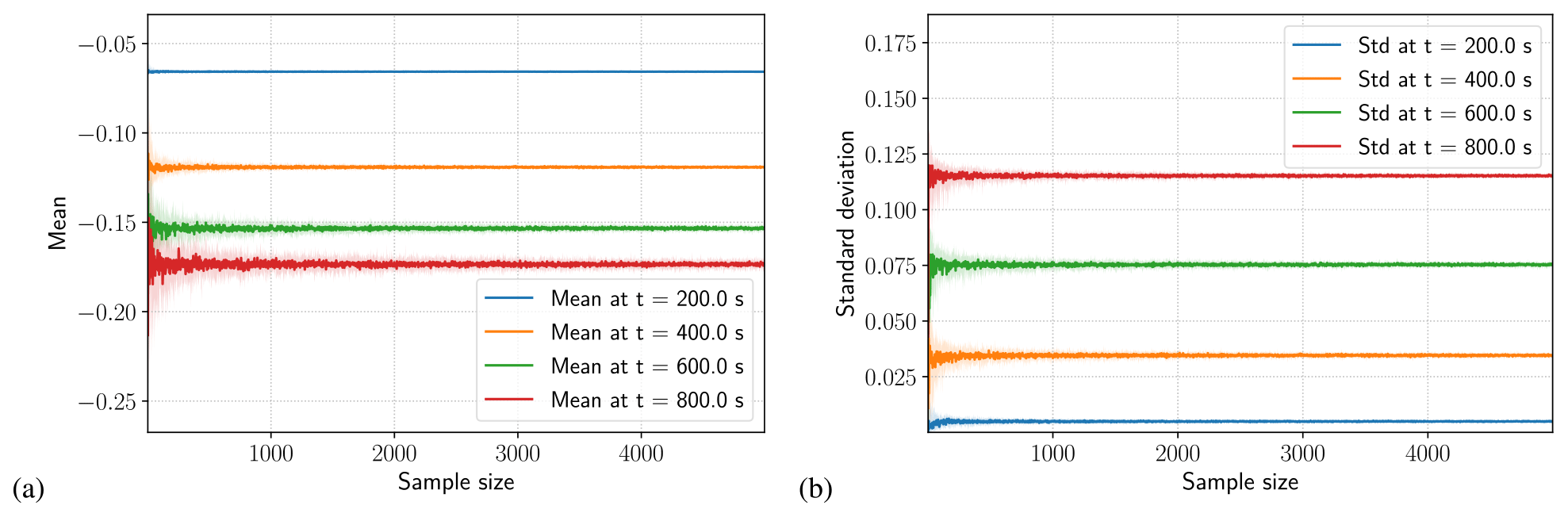
Figure C1 Mean and standard deviation convergence for case 1 for temperature (a) and frazil (b).

Figure C2 First-order Sobol index convergence for case 1 for temperature (a) and frazil (b).

Appendix D: Sobol indices and aggregated Sobol indices

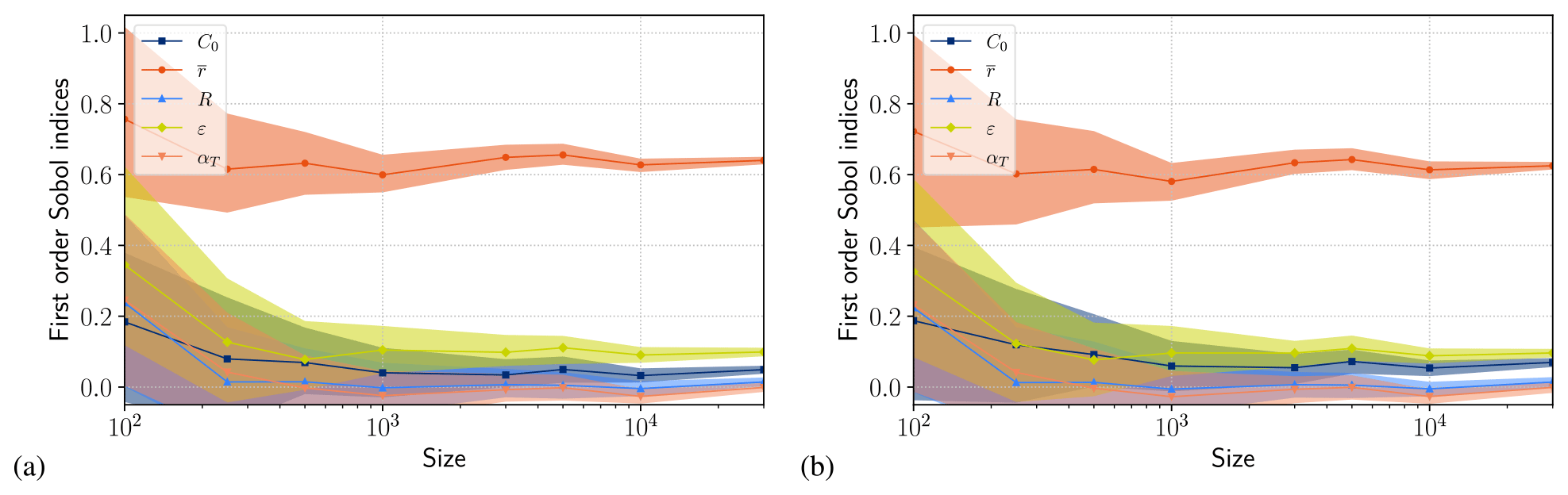
Figure D1 First-order and total-order Sobol indices at times t_min, 2t_min and t_f and aggregated Sobol indices for temperature (left panels) and frazil (right panels) for case 1 (a), 2 (b), 3 (c) and 4 (d) from top to bottom.

Appendix E: Aggregated Sobol indices

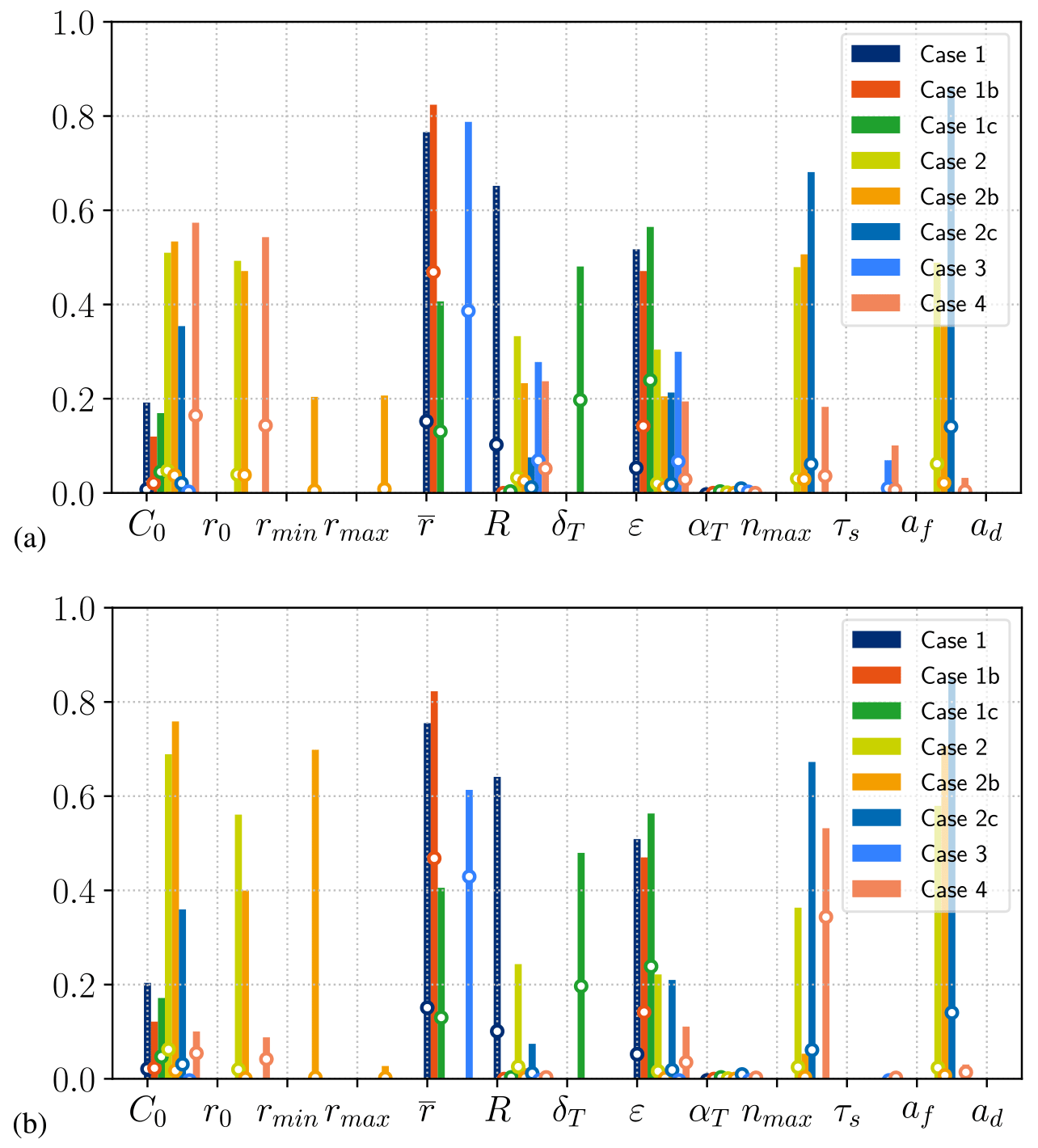
Figure E1 Aggregated first-order Sobol indices (dots) and aggregated total Sobol indices (bars) for temperature (a) and total frazil volume fraction (b) for case 1, 1b, 1c, 2, 2b, 2c, 3 and 4.

Appendix F: Results of case 1

Figure F1 Results of case 1. From top to bottom: uncertainty propagation result (a), first-order Sobol indices (b), first-order Sobol indices with 95 % confidence intervals (c), and total-order Sobol indices with 95 % confidence intervals (d) for temperature (left panels) and frazil (right panels).

Appendix G: Results of case 2

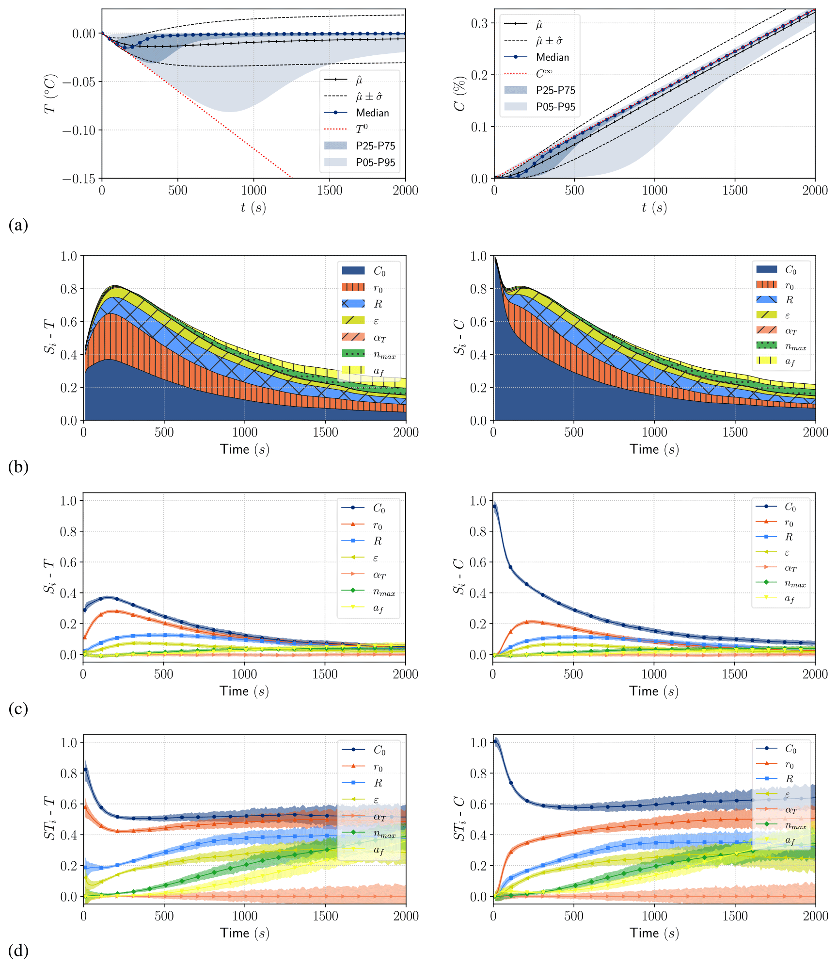
Figure G1 Results of case 2. From top to bottom: uncertainty propagation result (a), first-order Sobol indices (b), first-order Sobol indices with 95 % confidence intervals (c), and total-order Sobol indices with 95 % confidence intervals (d) for temperature (left panels) and frazil (right panels).

Appendix H: Results of case 3

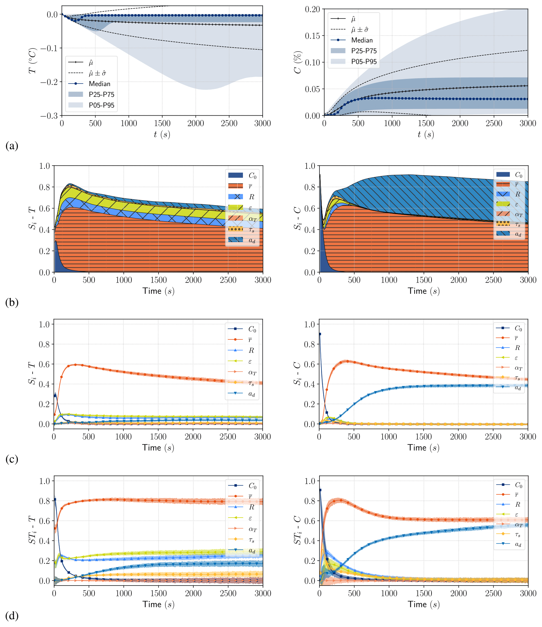
Figure H1 Results of case 3. From top to bottom: uncertainty propagation result (a), first-order Sobol indices (b), first-order Sobol indices with 95 % confidence intervals (c), and total-order Sobol indices with 95 % confidence intervals (d) for temperature (left panels) and frazil (right panels).

Appendix I: Results of case 4

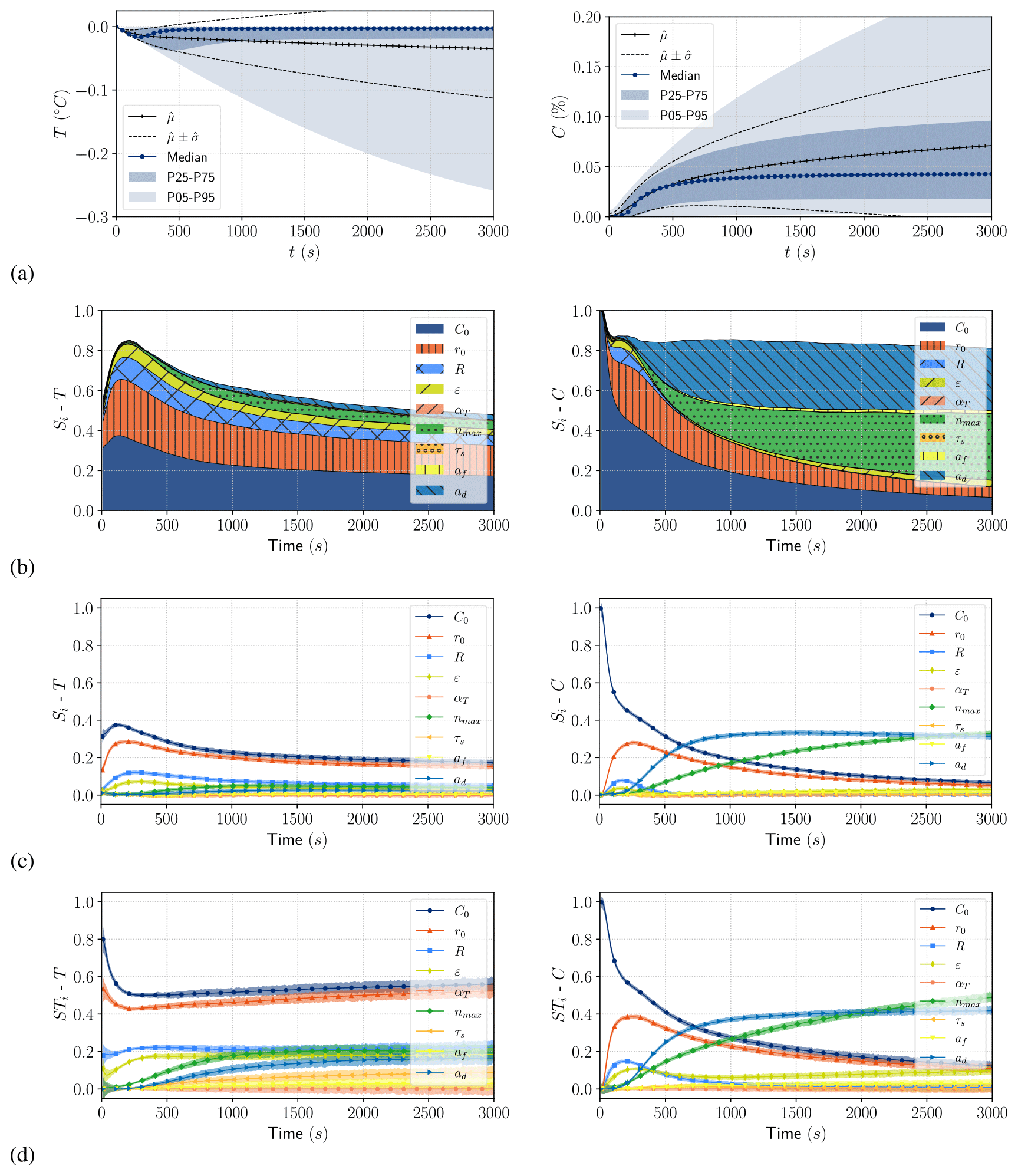
Figure I1 Results of case 4. From top to bottom: uncertainty propagation result (a), first-order Sobol indices (b), first-order Sobol indices with 95 % confidence intervals (c), and total-order Sobol indices with 95 % confidence intervals (d) for temperature (left panels) and frazil (right panels).